Non-Deterministic Policy Improvement
Stabilizes Approximated Reinforcement Learning

Abstract

This paper investigates a type of instability that is linked to the greedy policy improvement in approximated reinforcement learning. We show empirically that non-deterministic policy improvement can stabilize methods like LSPI by controlling the improvements’ stochasticity. Additionally we show that a suitable representation of the value function also stabilizes the solution to some degree. The presented approach is simple and should also be easily transferable to more sophisticated algorithms like deep reinforcement learning.

Keywords: stability, approximate reinforcement learning, non-deterministic policy improvement, least-squares policy iteration, slow-feature-analysis representation

1 Introduction

This paper investigates a type of instability that is linked to the greedy policy improvement in approximated reinforcement learning. We show empirically that non-deterministic policy improvement can be used to achieve stability for large discount factors. The presented approach is simple and should also be easily transferable to more sophisticated algorithms.

Recently deep reinforcement learning (deep RL) has been very successful in solving complex tasks in large, often continuous state spaces (e.g. playing Atari games and Go, Mnih et al., 2015; Silver et al., 2016). These approaches use gradient based Q-learning (Watkins and Dayan, 1992) or policy gradient methods (Williams, 1992). Gradients in neural networks must be based on i.i.d. distributed samples, though (see Riedmiller, 2005). Deep RL uses therefore mini-batches that are sampled i.i.d. from a fixed set of experiences, which has been collected before training (called experience replay, Mnih et al., 2013).

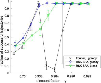
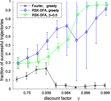
In difference to online algorithms, which are often guaranteed to converge in the limit of an infinite training sequence (e.g. Sutton et al., 2009), batch learning has long been known to be vulnerable to the choice of training sets (Tsitsiklis and Van Roy, 1997; Bertsekas, 2007). Depending on the batch of training samples at hand, an RL algorithm can either converge to an almost optimal or to an arbitrarily bad policy. In practice, this depends strongly (but not predictably) on the discount factor $\gamma$. For example, in Figure 1 we demonstrate that policies learned by least-squares policy iteration (LSPI, Lagoudakis and Parr, 2003) yield very different performances when the discount factor $\gamma$ is varied (experimental details can be found in Section 3). The left plot shows an unpredictable drop in performance for a simple navigation experiment with continuous states and discrete actions, and the right plot the failure of LSPI to learn a suitable policy for a more complicated environment. The young discipline of deep RL has not yet reported effects like these, but it is reasonable to assume that they happen in batch algorithms with more sophisticated architectures as well.

Figure 1: Navigation performance of policies, learned by LSPI in two environments (see sketched layouts), for varying discount factors $\gamma$. Error bars indicate mean and standard deviation of the fraction of successful test-trajectories (starting at random positions) over 10 random-walk training sets with 50000 samples each. The agent can either move forward or rotate 45^∘ left or right (i.e. 3 actions). Reaching the goal area is rewarded (+1) and crashing into a wall is punished (-1 or -10).

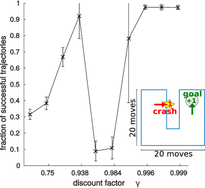
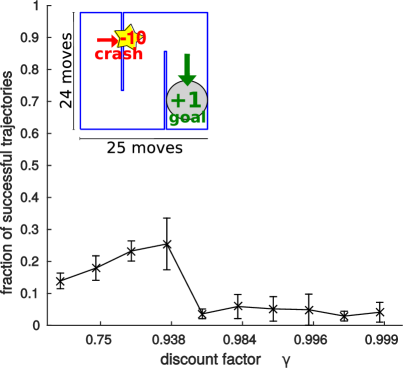
Most authors attribute this instability to a lack of convergence guarantees in off-policy batch value estimation (see Dann et al., 2014, for an overview). But the distribution of training samples in the batch may also have a profound impact on the policy improvement in approximate RL. For example, Perkins and Precup (2002) show for an algorithm similar to LSPI, that the greedy policy improvement can cause the instability shown in Figure 1. Although their analysis does not carry over to LSPI, they show that a sequence of non-deterministic policies converge reliably when they are changed slowly enough. Conservative policy iteration (CPI, Kakade and Langford, 2002) follows a similar line of thought and slows down the policy improvement considerably to guarantee convergence. Safe policy iteration (SPI, Pirotta et al., 2013) extends this concept by determining the speed of change through a lower bound on the policy improvement. The algorithm improves convergence speed significantly, but is computationally expensive even in finite state spaces. Other approaches suggest an actor-critic architecture to avoid oscillations (Wagner, 2011) or optimize a parameterizable softmax-policy directly (Azar et al., 2012).

In this paper we evaluate the idea of Perkins and Precup (2002) empirically with LSPI in continuous navigation tasks. Surprisingly, we find that the stochasticity of the improved policy stabilizes the solution, rather than the slowness of policy change. This requires only a small modification to the policy improvement scheme. Although our approach is a heuristic and theoretically not as well-grounded as the above algorithms, it is fast, simple to implement, and can be applied to most algorithms used in deep RL.

2 Non-Deterministic Policy Improvement

In this paper we consider tasks with continuous state space $\mathcal{X}$ and discrete action space $\mathcal{A}$. A non-deterministic policy $\pi(a|x)\in[0,1]\,,\forall a\in\mathcal{A}\,,\sum_{a^{\prime}\in\mathcal{A}}\pi(a^{\prime}|x)=1\,,\forall x\in\mathcal{X}\,,$ can be evaluated by any algorithm to estimate the corresponding Q-value function $q:\mathcal{X}\times\mathcal{A}\to\mathrm{I\kern-1.72218ptR}$. To converge to the optimal policy, the policy $\pi$ must also be improved, either during Q-value estimation or in an additional step. The improvement in a state $x\in\mathcal{X}$ usually chooses the action $a\in\mathcal{A}$ that maximizes the current Q-value estimate $q(x,a)$. Instead of this greedy improvement, we propose to produce an improved non-deterministic policy. Examples are softmax $\pi_{\beta}^{q}$ or $\epsilon$-greedy $\pi_{\epsilon}^{q}$ policies, that is, $\forall a\in\mathcal{A},\forall x\in\mathcal{X}$:

$$\pi_{\beta}^{q}(a|x)=\frac{\exp\big{(}\beta\,q(x,a)\big{)}}{\sum\limits_{a^{\prime}\in\mathcal{A}}\exp\big{(}\beta\,q(x,a^{\prime})\big{)}}\quad\;\;\text{or}\quad\;\;\pi_{\epsilon}^{q}(a|x)=\epsilon\,{\textstyle\frac{1}{|\mathcal{A}|}}+\left\{\begin{array}[]{cl}1-\epsilon&\kern-6.45831pt,\text{if}\,a=\operatorname*{\text{\rm arg}\,\text{\rm max}}\limits_{a^{\prime}\in\mathcal{A}}q(x,a^{\prime})\\ 0&\kern-6.45831pt,\text{otherwise}\end{array}\right.\,.$$

Existing algorithms can be adapted by identifying the greedy policy improvement operator ${\rm\hat{\Gamma}}{\kern-2.15277pt_{*}}$ and replacing it with the non-deterministic ${\rm\hat{\Gamma}}{\kern-2.15277pt_{\beta}}$, that is, for functions $f,q:\mathcal{X}\times\mathcal{A}\to\mathrm{I\kern-1.72218ptR}$:

$${\rm\hat{\Gamma}}{\kern-2.15277pt_{*}}[f|q](x)\;=\;f\big{(}x,\operatorname*{\text{\rm arg}\,\text{\rm max}}_{a\in\mathcal{A}}q(x,a)\big{)}\quad\;\Rightarrow\quad\;{\rm\hat{\Gamma}}{\kern-2.15277pt_{\beta}}[f|q](x)\;=\;\sum_{a\in\mathcal{A}}\pi_{\beta}^{q}(a|x)\,f(x,a)\,,\qquad\forall x\in\mathcal{X}\,.$$

Here $\beta\in[0,\infty)$ denotes the inverse stochasticity of the operator. For example, a non-deterministic version of the TD-error $\delta_{t}$ in Q-learning for the observation $(x_{t},a_{t},r_{t},x_{t+1})$ is $\delta_{t}=r_{t}+\gamma\,{\rm\hat{\Gamma}}{\kern-2.15277pt_{\beta}}[q|q](x_{t+1})-q(x_{t},a_{t})$, and the matrix $\mathbf{A}\in\mathrm{I\kern-1.72218ptR}^{m\times m}$, which has to be inverted during non-deterministic least-squares temporal difference learning (LSTD, Bradtke and Barto, 1996, used by LSPI), would be computed from a training batch $\{x_{t},a_{t},r_{t}\}_{t=0}^{n}$ by

$$A_{ij}\;\;=\;\;{\textstyle\frac{1}{n}}{\textstyle\sum\limits_{\scriptscriptstyle t=0}^{\scriptscriptstyle n-1}}\phi_{i}(x_{t},a_{t})\Big{(}\phi_{j}(x_{t},a_{t})-\gamma{\rm\hat{\Gamma}}{\kern-2.15277pt_{\beta}}[\phi_{j}|q](x_{t+1})\Big{)}\,,\qquad\forall i,j\in\{1,\ldots,m\}\,.$$

Softmax policies use more information than $\epsilon$-greedy and are in most situations the better choice. However, the stochasticity of the softmax depends strongly on the differences between Q-values. Far away from the reward, Q-values can become very similar and softmax policies become almost uniform distributions. The level of stochasticity turns out to be the most reliable stabilizer for LSPI, and we used in our experiments (see Section 3) normalized Q-values $\bar{q}$ for non-deterministic policy improvement ${\rm\hat{\Gamma}}{\kern-2.15277pt_{\beta}}[f|\bar{q}]$. This normalizes the stochasticity for all states by normalizing the difference between Q-values, that is, $\forall x\in\mathcal{X},\forall a\in\mathcal{A}$:

$$\bar{q}(x,a)=\frac{q(x,a)-\mu(x)}{\sigma(x)}\,,\quad\mu(x)={\textstyle\frac{1}{|\mathcal{A}|}}{\textstyle\sum\limits_{\scriptscriptstyle a^{\prime}\in\mathcal{A}}}q(x,a^{\prime})\,,\quad\sigma(x)=\sqrt{{\textstyle\frac{1}{|\mathcal{A}|}}{\textstyle\sum\limits_{\scriptscriptstyle a^{\prime}\in\mathcal{A}}}\big{(}q(x,a^{\prime})\big{)}^{2}-\big{(}\mu(x)\big{)}^{2}}\,.$$

3 Experiments

We evaluated the effects of non-deterministic policy improvement at the example of a simple navigation experiment in an U- and a S-shaped environment (see inlays of Figure 1). The three dimensional state space $\mathcal{X}$ consisted of the agent’s two-dimensional position and its orientation. The action space $\mathcal{A}$ contained 3 actions: a forward movement and two 45^∘ rotations. Crashing into a wall stopped movement and it would take the agent between 20 and 25 unimpeded moves to traverse the environment in one spatial dimension. Reaching the goal area (gray circle in the inlays) yielded a reward of +1 and crashes incurred a punishment of -1 in the U-shaped and -10 in the S-shaped environment. To represent the Q-value function, we chose a Fourier basis (Konidaris et al., 2011) and constructed 1500 basis functions over the space of states and actions. The bases contained all combinations of: 10 cosine functions (including a constant) for each spatial dimension; a constant, 2 cosine and 2 sine functions for the orientation; and 3 discrete Kronecker-delta functions for the actions. Irrespective their policy improvement, policies were evaluated greedily to remain comparable. Performance was measured in fraction of successful trajectories, which we estimated by running the greedy policy from 200 random starting positions/orientations. Successful trajectories reach the goal within 100 actions without hitting a wall.

Figure 2: LSPI with greedy and softmax policy improvement, compared in the navigation tasks of Figure 1. Large standard deviations are usually caused by a mixture of excellent and horrible policies. We therefore call these regimes “instable”. Stochastic improvements (with small $\beta$, e.g. green triangles) decrease performance for small $\gamma$, but stabilize convergence for large $\gamma$ significantly.

Figure 3: LSPI policies based on different representations in the navigation tasks of Figure 1. Better representations (here RSK-SFA) generally improve performance, but non-deterministic policy improvement is still needed to stabilize LSPI in complex tasks (e.g., right plot). Also note the pronounced trade-off between $\beta$ and $\gamma$.

3.1 Non-Deterministic Policy Improvement

We started out to test the idea of Perkins and Precup (2002) for LSPI by using non-deterministic policy improvement (soft-LSPI) with slowly growing inverse stochasticity $\beta$ (similar to simulated annealing, Haykin, 1998). However, we observed that the annealing process itself did not improve the learned policy. The performance was always comparable to soft-LSPI with the annealing’s final stochasticity $\beta$ (not shown here).

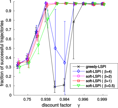
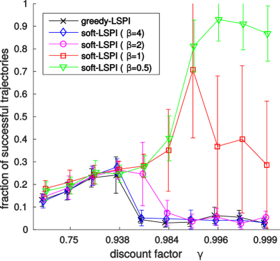
Figure 2 plots the performance of greedy-LSPI and soft-LSPI (with constant stochasticity $\beta$) for varying discount factors $\gamma$. In the face of sparse rewards, $\gamma$ determines how far that reward is propagated, before it is drowned in inevitable approximation errors. Low $\gamma$ yields policies that are only correct close to the reward, and have therefore a bad performance. On the other hand, $\gamma$ close to 1 can lead to nearly optimal policies everywhere, but performance is strongly affected by the instability investigated in this paper. Note that the large standard deviations in both plots stem from some training sets producing near optimal, while others producing nonsensical policies. For this reason we refer to these regimes as “instable”. First, one can observe that increasing stochasticity (lower $\beta$) drastically stabilizes the soft-LSPI policies. Secondly, note that there seems to be a trade-off between inverse stochasticity $\beta$ and discount factor $\gamma$. Low $\beta$ reduces performance while increasing stability, but in the left plot the performance with low $\beta$ becomes near optimal for larger $\gamma$, too. It appears therefore that instabilities can generally be counteracted by simultaneously lowering $\beta$ and raising $\gamma$.

3.2 Stabilization by Representation

So far the above instabilities have only been demonstrated for LSPI. One could argue that more sophisticated approaches must not be affected in the same way. In deep neural networks, for example, the lower layers may provide a representation of the state-action space that stabilizes policy improvement. We want to investigate this by choosing basis functions, which are known to represent value functions well. Böhmer et al. (2013) show that features learned by non-linear slow feature analysis (SFA, Wiskott and Sejnowski, 2002) approximate an optimal encoding for value functions of all tasks in the same environment. We used regularized sparse kernel SFA (RSK-SFA, Böhmer et al., 2012) with Gaussian kernels to learn such features from the training data. Figure 3 shows the results in comparison with the trigonometric Fourier basis functions introduced above. Using the SFA representation completely avoided instability for the simpler task in the left plot (blue diamonds). The performance improves in the S-shaped environment too, but the large standard deviations indicate that here greedy LSPI is not very stable for large discount factors $\gamma$. Soft-LSPI with a low $\beta$ (green triangles) stabilizes the solution, though. Using a deep architecture may therefore reduce instability, but will probably not remove it all together. Nonetheless, our results suggest that non-deterministic policy improvement should be able to stabilize deep architectures, too.

4 Conclusion

We have shown that (at least) LSPI can become instable in some unpredictable regimes of the discount factor $\gamma$. Here small differences in the training set can lead to large differences in policy performance. It is not exactly clear why solutions become instable, but we show that learned policies can be stabilized by using a non-deterministic policy improvement scheme. All presented experiments became significantly more stable by increasing stochasticity $\frac{1}{\beta}$ and discount factor $\gamma$ at the same time. Future works may extend our approach by adjusting both parameters during policy iteration (like in SPI, Pirotta et al., 2013). Better representations of the state-action space have also improved stability to some extend. More sophisticated approaches (like deep RL) learn these representations implicitly in their lower layers and may therefore be more stable than LSPI. Nonetheless, instabilities will probably occur, and non-deterministic policy improvement can most likely be employed to stabilize the learned policy in deep RL, too.

In conclusion, when success or failure of learned policies depends crucially on the training set (e.g. during cross-validation), one should consider a non-deterministic policy improvement scheme. The scheme presented in this paper is computationally cheap, easy to implement, and can be fine-tuned with the inverse stochasticity $\beta$.

Acknowledgments

We thank the anonymous reviewers, who pointed us in the direction of CPI. This work was funded by the German science foundation (DFG) within SPP 1527 autonomous learning.

References

- Azar et al. (2012) Mohammad Gheshlaghi Azar, Vicenç Gómez, and Hilbert J. Kappen. Dynamic policy programming. Journal of Machine Learning Research, 13:3207–3245, 2012.
- Bertsekas (2007) Dimitri P. Bertsekas. Dynamic Programming and Optimal Control, volume 2. Athena Scientific, 3rd edition, 2007.
- Böhmer et al. (2012) Wendelin Böhmer, Steffen Grünewälder, Hannes Nickisch, and Klaus Obermayer. Generating feature spaces for linear algorithms with regularized sparse kernel slow feature analysis. Machine Learning, 89(1-2):67–86, 2012.
- Böhmer et al. (2013) Wendelin Böhmer, Steffen Grünewälder, Yun Shen, Marek Musial, and Klaus Obermayer. Construction of approximation spaces for reinforcement learning. Journal of Machine Learning Research, 14:2067–2118, July 2013.
- Bradtke and Barto (1996) Steven J. Bradtke and Aandrew G. Barto. Linear least-squares algorithms for temporal difference learning. Machine Learning, 22(1/2/3):33–57, 1996.
- Dann et al. (2014) Christoph Dann, Gerhard Neumann, and Jan Peters. Policy evaluation with temporal differences: a survey and comparison. Journal of Machine Learning Research, 15:809–883, 2014.
- Haykin (1998) Simon Haykin. Neural Networks: A Comprehensive Foundation. Prentice Hall, 2nd edition, 1998. ISBN 978-0132733502.
- Kakade and Langford (2002) Sham Kakade and John Langford. Approximately optimal approximate reinforcement learning. In Proceedings of the 19th International Conference on Machine Learning, pages 267–274, 2002.
- Konidaris et al. (2011) G. D. Konidaris, S. Osentoski, and P.S. Thomas. Value function approximation in reinforcement learning using the Fourier basis. In Proceedings of the Twenty-Fifth Conference on Artificial Intelligence, 2011.
- Lagoudakis and Parr (2003) Michail G. Lagoudakis and Ronald Parr. Least-squares policy iteration. Journal of Machine Learning Research, 4:1107–1149, 2003.
- Mnih et al. (2013) Volodymyr Mnih, Koray Kavukcuoglu, David Silver, Alex Graves, Ioannis Antonoglou, Daan Wierstra, and Martin Riedmiller. Playing Atari with deep reinforcement learning. In NIPS Deep Learning Workshop. 2013.
- Mnih et al. (2015) Volodymyr Mnih, Koray Kavukcuoglu, David Silver, Andrei A. Rusu, Joel Veness, Marc G. Bellemare, Alex Graves, Martin Riedmiller, Andreas K. Fidjeland, Georg Ostrovski, Stig Petersen, Charles Beattie, Amir Sadik, Ioannis Antonoglou, Helen King, Dharshan Kumaran, Daan Wierstra, Shane Legg, and Demis Hassabis. Human-level control through deep reinforcement learning. Nature, 518(7540):529–533, February 2015.
- Perkins and Precup (2002) Theodore J. Perkins and Doina Precup. A convergent form of approximate policy iteration. In Advances in Neural Information Processing Systems 15, pages 1595–1602. 2002.
- Pirotta et al. (2013) Matteo Pirotta, Marcello Restelli, Alessio Pecorino, and Daniele Calandriello. Safe policy iteration. In Proceedings of the 30th International Conference on Machine Learning, pages 307–315, 2013.
- Riedmiller (2005) Martin Riedmiller. Neural fitted Q-iteration - first experiences with a data efficient neural reinforcement learning method. In 16th European Conference on Machine Learning, pages 317–328. Springer, 2005.
- Silver et al. (2016) David Silver, Aja Huang, Christopher J. Maddison, Arthur Guez, Laurent Sifre, George van den Driessche, Julian Schrittwieser, Ioannis Antonoglou, Veda Panneershelvam, Marc Lanctot, Sander Dieleman, Dominik Grewe, John Nham, Nal Kalchbrenner, Ilya Sutskever, Timothy Lillicrap, Madeleine Leach, Koray Kavukcuoglu, Thore Graepel, and Demis Hassabis. Mastering the game of Go with deep neural networks and tree search. Nature, 529:484–503, January 2016.
- Sutton et al. (2009) Richard S. Sutton, Csaba Szepesvári, and Hamid Reza Maei. A convergent algorithm for off-policy temporal-difference learning with linear function approximation. In Advances in Neural Information Processing Systems, volume 21, pages 1609–1616. MIT Press, 2009.
- Tsitsiklis and Van Roy (1997) John N. Tsitsiklis and Benjamin Van Roy. An analysis of temporal-difference learning with function approximation. IEEE Transactions on Automatic Control, 42(5):674–690, 1997.
- Wagner (2011) Paul Wagner. A reinterpretation of the policy oscillation phenomenon in approximate policy iteration. In Advances in Neural Information Processing Systems 24, pages 2573–2581. 2011.
- Watkins and Dayan (1992) Christopher Watkins and Peter Dayan. Q-learning. Machine Learning, 8:279–292, 1992.
- Williams (1992) Ronald J. Williams. Simple statistical gradient-following algorithms for connectionist reinforcement learning. Machine Learning, 8(3):229–256, 1992.
- Wiskott and Sejnowski (2002) Laurenz Wiskott and Terrence Sejnowski. Slow feature analysis: unsupervised learning of invariances. Neural Computation, 14(4):715–770, 2002.