A Revisit of Hashing Algorithms for Approximate Nearest Neighbor Search

Abstract

Approximate Nearest Neighbor Search (ANNS) is a fundamental problem in many areas of machine learning and data mining. During the past decade, numerous hashing algorithms are proposed to solve this problem. Every proposed algorithm claims to outperform Locality Sensitive Hashing (LSH) which is the most popular hashing method. However, the evaluation of these hashing papers was not thorough enough, and the claim should be re-examined. The ultimate goal of an ANNS method is returning the most accurate answers (nearest neighbors) in the shortest time. If implemented correctly, almost all the hashing methods will have their performance improved as the code length increases. However, many existing hashing papers only report the performance with the code length shorter than 128. In this paper, we carefully revisit the problem of search with a hash index and analyze the pros and cons of two popular hash index search procedures. Then we proposed a very simple but effective two-level index structure and made a thorough comparison of eleven popular hashing algorithms. Surprisingly, the random-projection-based Locality Sensitive Hashing (LSH) ranked the first, which is in contradiction to the claims in all the other ten hashing papers. Despite the extreme simplicity of random-projection-based LSH, our results show that the capability of this algorithm has been far underestimated. For the sake of reproducibility, all the codes used in the paper are released on GitHub, which can be used as a testing platform for a fair comparison between various hashing algorithms.

1 Introduction

Nearest neighbor search plays an important role in many applications of machine learning and data mining. Given a dataset with $N$ entries, the cost of finding the exact nearest neighbor is $O(N)$, which is very time consuming when the data set is large. So people turn to Approximate Nearest Neighbor (ANN) search in practice [1, 22]. Hierarchical structure (tree) based methods, such as KD-tree [4] ,Randomized KD-tree [36], K-means tree [8], are popular solutions for the ANN search problem. These methods perform very well when the dimension of the data is relatively low. However, the performance decreases dramatically as the dimension of the data increases [39].

During the past decade, hashing based ANN search methods [10, 41, 25] received considerable attention. These methods generate binary codes for high dimensional data points (real vectors) and try to preserve the similarity among the original real vectors. A hashing algorithm generating $l$-bits code can be regarded as contains $l$ hash functions. Each function partitions the original feature space into two parts, the points in one part are coded as 1, and the points in the other part are coded as 0. When an $l$-bits code is used, the hashing algorithm ($l$ hash functions) partitions the feature space into $2^{l}$ parts, which can be named as hash buckets. Thus, all the data points fall into different hash buckets (associated with different binary codes). Ideally, if neighbor vectors fall into the same bucket or the nearby buckets (measured by the Hamming distance of binary codes), the hashing based methods can efficiently retrieve the nearest neighbors of a query point.

One of the most popular hashing algorithms is Locality Sensitive Hashing (LSH) [15, 10]. LSH is a name for a set of hashing algorithms, and we can specifically design different LSH algorithms for different types of data [10]. For real vectors, random-projection-based LSH [5] might be the most simple and popular one. This algorithm uses random projection to partition the feature space.

LSH is naturally data independent. Many data-dependent hashing algorithms [41, 25, 24, 37, 44, 12, 11, 20, 43, 31, 35, 16, 30, 14, 40, 23, 27, 13, 9, 17, 42, 18, 21, 29] have been proposed during the past decades and all these algorithms claimed to have superior performance over the baseline algorithm LSH. However, the evaluation of all these papers are not thorough enough, and their conclusions are questionable:

• How to measure the performance of the learned binary code might be the most critical problem in designing a new hashing algorithm. A straightforward answer could be using the binary code as the index to solve the ANNS problem. The ANNS performance can then be used to evaluate the performance of the binary code. However, there are two typical procedures for search with a hash index, the “hamming ranking” approach and the “hash bucket search” approach. Each approach has its pros and cons. For different datasets, different hashing algorithms favour different approaches. It is not easy to fairly compare different hashing algorithms.

• Most of the existing hashing paper [41, 25, 24, 37, 44, 12, 43, 31, 16, 30, 40, 27, 13, 9, 17, 42, 18, 21, 29] uses the ”hamming ranking” approach to examine the performance of various hashing algorithms. Since there are no publicly available c++ codes, all these papers use Matlab function and the accuracy - # of located samples curves to compare different hashing algorithms. Thus, different hashing algorithms should be compared with the same code length, and it is impossible to compare the hashing algorithms with various non-hashing based ANNS methods.

• Almost all the hashing papers report that the performance increases as the code length increases. However, most of the hashing papers [41, 25, 24, 37, 44, 12, 43, 31, 16, 30, 40, 27, 13, 9, 17, 42, 18, 21, 29] only reported the performance with the code length shorter than 128. How about we further increase the code length?

• Another possible approach to search with a hash index is so-called “hash bucket search” approach. Different from the “hamming ranking” approach, “hash bucket search” requires sophisticated data structures. If the hash bucket search approach is used, # of located samples is no longer a good indicator of the search time, and the accuracy - # of located samples curves become meaningless.

• Besides the “hamming ranking” and the “hash bucket search” approaches, can we design better hash index search procedure so that different hashing algorithms can be fairly and easily compared?

These problems have already been raised in the literature. Joly and Buisson [20] pointed out that many data-dependent hashing algorithms have the improvements over LSH, but ”improvements occur only for relatively small hash code sizes up to 64 or 128 bits”. The figure 4 in this paper [20] shows that when 1,024-bits codes were used, LSH is the best-performed hashing algorithm. However, Joly and Buisson [20] failed to provide a detailed analysis.

There is also a public available c++ program named FALCONN on the GitHub which implements LSH algorithm. Since we can record the search time of the program, the FALCONN (LSH) can be fairly compared with other non-hashing based ANNS methods. However, the results are not very encouraging. There are even researchers pointing out that ”LSH is so hopelessly slow and/or inaccurate”. Is this true that ”LSH is so hopelessly slow and/or inaccurate”?

All these problems motivate us to revisit the problem of applying hashing algorithms for ANNS. This study is carried on two popular million-scale ANNS datasets (SIFT1M and GIST1M), and the findings are very surprising:

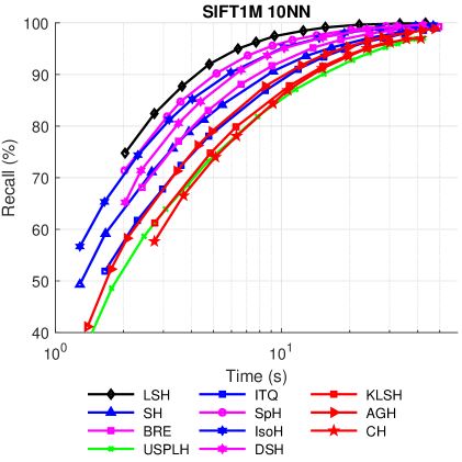
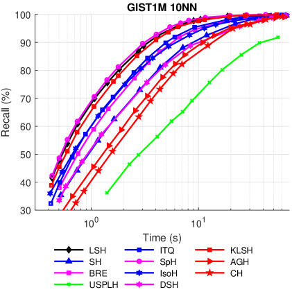
• Eleven popular hashing algorithms are thoroughly compared on these two datasets. Despite the fact that all the other ten data dependent hashing algorithms claimed the superiority over LSH which is data independent, LSH ranked the first among all the eleven compared algorithms on SIFT1M and ranked the second on GIST1M.

• We also compare our implementation of random-projection-based LSH (RPLSH) with other five popular open source ANNS algorithms (FALCONN, flann, annoy, faiss and KGrpah). On GIST1M, RPLSH performs best among the six compared methods. On SIFT1M, RPLSH performs the second best, and if a high recall is required (higher than 99%), RPLSH performs the best.

Despite the extreme simplicity of the random-projection-based LSH, our results show that the capability of this algorithm has been far underestimated. For the sake of reproducibility, all the codes are released on GitHub which can be used as a testing platform for a fair comparison between various hashing algorithms.

It is worthwhile to highlight the contributions of this paper:

• The goal of this paper is not introducing yet another hashing algorithm. We aim at providing analysis on how to correctly measure the performance of a hashing algorithm. Given the fact that almost all the existing hashing papers [41, 25, 24, 37, 44, 12, 43, 31, 16, 30, 40, 27, 13, 9, 17, 42, 18, 21, 29] failed to address this problem and gave misleading conclusions, we believe such analysis is important and useful.

• We introduce a simple yet novel two-level index scheme to search with a hash index. This approach significantly outperforms the traditional hamming ranking and the hash bucket search approaches. With this novel search approach, it becomes easy to compare various hashing algorithms fairly.

• We release an open source ANNS library RPLSH which implements this two-level index scheme with random-projection-based LSH. The comparison with other five popular open source ANNS algorithms (FALCONN, flann, annoy, faiss and KGraph) demonstrate the superiority of RPLSH. It performs the best on GIST1M and performs the second best on SIFT1M.

• Recently, graph-based algorithms [3, 33, 26, 7] have shown very promising performance on the ANNS problem. Besides KGraph, we do not compare with other more advanced graph-based algorithms. We agree that the performance of RPLSH is inferior to the performance of some graph-based algorithms (e.g., HNSW[33], NSG[7]) on CPU. However, RPLSH has its own advantages: very small index size, very efficient indexing and very simple search procedure. In some cases the graph-based algorithms cannot be used, RPLSH is a good choice. For example, RPLSH is very suitable for GPU, our study suggests the possibility of a GPU based ANNS algorithm which will outperform faiss (the current fastest GPU-based ANNS algorithm).

2 Search with A Hash Index

A hashing algorithm transforms the real vectors to binary codes. The binary codes can then be used as a hash index for online search. The general procedure of searching with a hash index is as follows (Suppose the user submit a query $q$ and ask for $K$ neighbors of the query):

1. The search system encodes the query to a binary code $b$ use the hash functions.

2. The search system finds $L$ points which are closest to $b$ in terms of the Hamming distance.

3. The search system performs a scan within the $L$ points, returns the top $K$ points which are closet to $q$.

This procedure is summarised in Algorithm 1, and there is one parameter $L$ which can be used to control the accuracy-efficiency trade-off. Based on this search procedure, we can see that the time of searching with a hash index contains three parts [19]:

Algorithm 1 Search with a hash index

1:base set D, query vector $q$, the hash functions, hash index (binary codes for all the points in the base set), the pool size $L$ and the number $K$ of required nearest neighbors,

2:$K$ points from the base set which are close to $q$.

3:Encode the query $q$ to a binary code $b$;

4:Locate $L$ points which have shortest hamming distance to $b$;

5:return the closet $K$ points to $q$ among these $L$ points.

1. Coding time $T_{c}$: the line 1 in Algorithm 1.

2. Locating time $T_{l}$: the lines 2 in Algorithm 1.

3. Scanning time $T_{s}$: the line 3 in Algorithm 1.

The total search time $T=T_{c}+T_{l}+T_{s}$. For many popular hashing algorithms, $T_{c}$ can be neglected compared to $T_{l}$ and $T_{s}$, please see Table V for details. $T_{s}$ is not related to the hashing algorithm and only depends on the parameter $L$. Thus, correctly measuring $T_{l}$ becomes the key to evaluate different hashing algorithms. There are two popular procedures (the hamming ranking approach and the hash bucket search approach) to complete the task in line 2. And these two approaches need significantly different $T_{l}$ for different hashing algorithms on different data set.

In the remaining part of this Section, we will analyze the pros and cons of two search procedures using the hash index. We will also experimentally verify our analysis. The experiments are performed on two popular ANNS datasets, SIFT1M and GIST1M. The basic statistics of these two datasets are shown in Table I.

TABLE I: Data sets

data set	dimension	base number	query number
SIFT1M	128	1,000,000	10,000
GIST1M	960	1,000,000	1,000

We use the random-projection-based LSH [5] for its simplicity. In the remaining part of this paper, the LSH algorithm we mentioned is this random-projection-based LSH.

Given a dataset with dimensionality $m$, one can generate an $m\times l$ random matrix from Gaussian distribution $\mathcal{N}(0,1)$ where $l$ is the required code length. Then the data will be projected onto $l$ dimensional space using this random matrix. The $l$ dimensional real representation of each point can then be converted to $l$-bits binary code by a simple binarize operation. The formal algorithm is illustrated in Algorithm (2).

Given a query point, the search algorithm is expected to return $K$ points. Then we need to examine how many points in this returned set are among the real $K$ nearest neighbors of the query. Suppose the returned set of $K$ points given a query is $R$ and the real $K$ nearest neighbors set of the query is $R^{\prime}$, the $precision$ and $recall$ can be defined [32] as

$$precision(R)=\frac{|R^{\prime}\cap R|}{|R|},\ \ \ recall(R)=\frac{|R^{\prime}\cap R|}{|R^{\prime}|}.$$ (1)

Since the sizes of $R^{\prime}$ and $R$ are the same, the recall and the precision of $R$ are actually the same. We fixed $K=100$ throughout our experiments.

Algorithm 2 random projection based LSH

1:base set D with $n$ $m$-dimensional points, code length $l$

2:$m\times l$ projection matrix $A$ and $n$ $l$-bits binary codes..

3:Generate an $m\times l$ random matrix $A$ from Gaussian distribution $\mathcal{N}(0,1)$;

4:Project the data onto $l$ dimensional space using this random matrix.

5:Convert the $n\times l$ dimensional data matrix to n $l$-bits binary codes by the binarize operation.

2.1 The Case That The Locating Time Being Ignored

Suppose we have an ideal approach which can locate $L$ binary vectors closest (measured by the hamming distance) to the query at no cost, i.e., the locating time $T_{l}$ can be ignored, the # of located samples, $L$, becomes a good indicator of the search time. Thus, the accuracy - # of located samples curve can used to compare the performance of different hashing algorithms.

(a) SIFT1M

(b) GIST1M

Figure 1: The recall - # of located samples curves of LSH on two datasets. We can see longer codes means better performance.

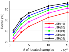
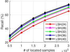
Figure 1 plots the recall - # of located samples curves of LSH on two datasets. The code length grows from 16 to 32 on SIFT1M and 24 to 40 on GIST1M. We can easily get the conclusion that longer code means better performance, which is a common conclusion in almost all the previous hashing papers [41, 25, 24, 37, 44, 12, 43, 31, 16, 30, 40, 27, 13, 9, 17, 42, 18, 21, 29].

This result is very natural and reasonable. Since each bit of the hash code is a partition of the feature space and same code (0 or 1) on this bit means two points are on the same side of this partition. If two points share $t$ bits same code, which means these two points are on the same sides of $t$ partitions. Neighbors in the hamming space with longer code are more likely to be the real neighbors in the original feature space. However, this is only valid when the locating time is ignored.

2.2 The Hamming Ranking Approach

The hamming ranking approach is very simple and wildly used in many hashing papers [41, 25, 24, 37, 44, 12, 43, 31, 16, 30, 40, 27, 13, 9, 17, 42, 18, 21, 29]. The algorithm procedure of hamming ranking can be found in Algorithm 3.

Algorithm 3 Hamming ranking approach for locate $L$ closest binary codes

1:Compute the hamming distances between $b$ and all the binary codes in the data set;

2:Sort the points based on the hamming distances in ascending order and keep the first $L$ points;

It is easy to find that the computational complexity of this approach is $O(N)$ where $N$ is the data points. Thus, the reason of using hash index (hamming ranking approach) to speed up search is that the computation of hamming distance of two binary codes can be extremely fast [38].

The locating time of hamming ranking approach (the time of Algorithm 3) is only determined by the code length and the parameter $L$. In other words, if two different hashing algorithms use the same code length and the same $L$, they will have the same locating time. Thus, we can compare different hashing algorithms with the same code length simply using the accuracy - # of located samples curves (ignore the locating time). This strategy is used in most of the exiting hashing papers [41, 25, 24, 37, 44, 12, 43, 31, 16, 30, 40, 27, 13, 9, 17, 42, 18, 21, 29]. Moreover, The locating time grows linearly with respect to the code length and the parameter $L$ (as shown in Figure 2).

Figure 2: The locating time complexity of the hamming ranking approach. (a) The locating time VS. the code length ($L=50,000$) (b) The locating time VS. the parameter $L$. The locating time grows linearly with respect to both the code length and the parameter $L$.

(a) SIFT1M

(b) GIST1M

Figure 3: The recall - search time curves of LSH using hamming ranking approach on two datasets.

Figure 4: The ANN search results of LSH with significant different code length on two datasets. The y-axis denotes the average recall while the x-axis denotes (a,b) the # of located samples (c,d) the search time using the hamming ranking approach.

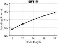
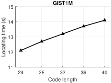
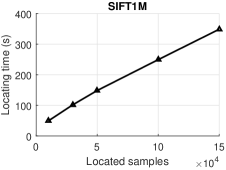
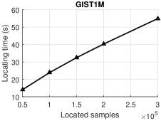
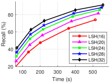
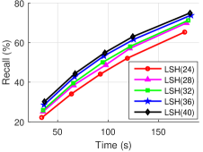
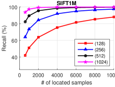
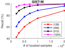
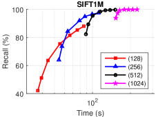
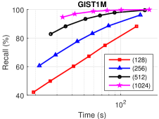
Figure 3 shows the recall - search time curves of LSH using hamming ranking approach on two datasets. This result is very similar to the result in Figure 1. It is because the locating time grows slowly as the code length increases and the code length differences between different curves in Figure 3 are also small. As the code length difference becomes larger, we can see the impact of the locating time, as shown in Figure 4.

One advantage of the hamming ranking approach is that the memory usage of the index is extremely small. From Algorithm 3, we can find that there is no additional data structure needed and we only need to store the binary codes for the data points in the database. Suppose the database contains $n$ data points and we use $l$ bits code, we need $n\frac{l}{8}$ byte. This memory usage may be the smallest one among most of the popular ANNS methods even when $l=1024$.

2.3 The Hash Bucket Search Approach

TABLE II: Hamming radius VS. # of queries successfully located 50000 points on SIFT1M (total # of queries 10,000)

hamming radius	0	1	2	3	4	5	6	7	8	9	10
# of buckets (16 bits)	1	16	120	560	1,820	4,368	8,008	11,440	12,870	11,440	8,008
# of queries (16 bits) (1.752s)	0	3637	4932	1230	169	30	1	1	0	0	0
# of buckets (32 bits)	1	32	496	4960	35,960	201,376	906,192	3,365,856	10,518,300	28,048,800	64,512,240
# of queries (32 bits) (237.8s)	0	0	0	4	1710	4282	2691	1021	241	44	7

TABLE III: Hamming radius VS. # of queries successfully located 50000 points on GIST1M (total # of queries 1,000)

hamming radius	0	1	2	3	4	5	6	7	8	9	10
# of buckets (24 bits)	1	24	276	2,024	10,626	42,504	134,596	346,104	735,471	1,307,504	1,961,256
# of queries (24 bits) (0.234s)	70	467	277	115	44	18	7	2	0	0	0
# of buckets (40 bits)	1	40	780	9,880	91,390	658,008	3,838,380	18,643,560	76,904,685	273,438,880	847,660,528
# of queries (40 bits) (240.0s)	0	0	27	252	302	205	107	57	27	14	9

Algorithm 4 Hash bucket search approach for locate $L$ closest binary codes

1:Let hamming radius $r=0$;

2:Let candidate pool set $C=\emptyset$;

3:while $|C|<L$ do

4:     Get the buckets list $B$ with hamming distance $r$ to $b$;

5:     for all bucket $bb$ in $B$ do

6:         Put all the points in $bb$ into $C$;

7:         if $|C|>=L$ then

8:              Keep the first $L$ points in $C$;

9:              return;

10:         end if

11:     end for

12:     $r=r+1$;

13:end while

(a) SIFT1M

(b) GIST1M

Figure 5: The recall - search time curves of LSH using hash bucket search approach on two datasets.

Figure 6: The locating time complexity of the hash bucket search approach. (a) The locating time VS. the code length ($L=50,000$) (b) The locating time VS. the parameter $L$. The locating time grows exponentially with respect to the code length and grows super-linearly with the parameter $L$.

The hash bucket search is another popular method to locate those nearest binary codes in the hamming space. The corresponding algorithm procedure can be found in Algorithm 4.

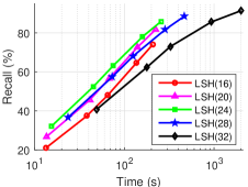
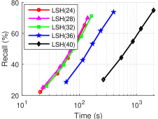
Figure 5 shows the recall - time curves using the hash bucket search approach of LSH on two datasets. These curves are significant different with the curves in Figure 1 and Figure 3. There is an optimal code length for hash bucket search approach (24 in SIFT1M and 28 in GIST1M). As the code length further increases, the search performance decreases significantly.

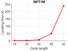
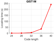
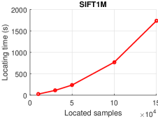
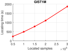
Given a binary code $b$, locating the hashing bucket corresponding to $b$ costs $O(1)$ time (by using std::vector). If there are enough points (larger than $L$) in this bucket, the total time cost of the hash bucket search is $O(1)$, which seems much more efficient than the hamming ranking approach. However, this is only true when the binary code is short. As the code length increases, the number of hash bucket increases exponentially. And there are always not enough points (even no point) in the bucket corresponding to the query. To locate $L$ points, We need to increase the hamming radius $r$. Given an $l$-bits code $b$, considering those hashing buckets whose Hamming distance to $b$ is smaller or equal to $r$. It is easy to show the number of these buckets is $\sum_{i=0}^{r}\binom{l}{i}$, which increases almost exponentially with respect to $r$ and $l$. As the $L$ increases, to locate $L$ points successfully, $r$ has to be increased. Overall, the locating time of the hash bucket search approach grows exponentially with respect to the code length $l$ and super-linearly with respect to the parameter $L$ (as shown in Figure 6).

Table II and III record the number of queries (the total number is 10,000 on SIFT1M and 1,000 on GIST1M) which successfully located 50,000 samples in different hamming radius with different code length with the hash bucket search approach. As the code length increases, the number of hash buckets corresponding to the same hamming radius increases almost exponentially. Moreover, as the code length increases, the base points are more diversified. Thus we need to increase the hamming radius to locate enough number of samples. These two reasons cause the locating time grows exponentially as the code length increases for the hash bucket search approach. As a result, the hash bucket search approach has no practical meaning if the code length is longer than 64.

However, Section 2.1 shows long codes can generate better search candidates. A natural question will be can we design a method for the hash bucket search approach to take the advantages of long codes?

The answer is yes. A straightforward way is using multiple hash tables to represent long codes. Suppose we have 128-bits codes and we use a single table with 128-bits. To locate $L$ points, if the points in all the buckets within the Hamming distance $r$ are not enough, we have to increase the hamming radius $r$. The locating time will then grow significantly and the extremely long locating time will make the hash bucket search approach meaningless. If we use four tables, each table is 32-bits. Instead of growing $r$, we can scan the buckets within the hamming radius $r$ in all the tables, which gives us a more substantial chance to locate enough data points.

(a) SIFT1M

(b) GIST1M

Figure 7: The recall-time curves of the hash bucket search approach with different number of tables on SIFT1M and GIST1M.

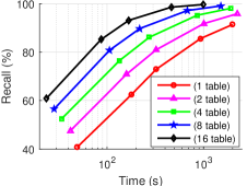
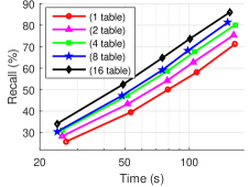
Figure 7 shows the recall-time curves of the hash bucket search approach on LSH code with the different number of tables (each table is 32-bits). The results are very consistent: the hash bucket search approach gains the advantage by using multiple tables on both datasets. This multiple tables trick is more effective on SIFT1M than on GIST1M.

With 1,024 bits code, we can use $\lceil\frac{1024}{w}\rceil$ tables, each table is $w\leq 1024$ bits. If we use the recall - time curve, the performance of the hash bucket search approach will firstly increase then dramatically decrease as the $w$ increases. There will be an optimal $w$ given a hashing algorithm and the dataset.

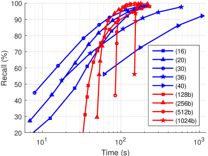
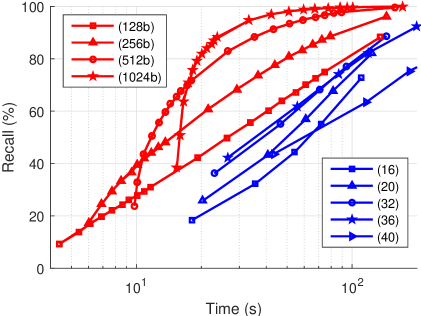
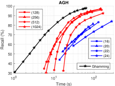
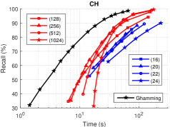
Figure 8 shows the performance of LSH on two datasets with both hamming ranking and hash bucket search approaches. We use 128, 256, 512 and 1024 bits for the hamming ranking approach. For the hash bucket search approach, we use $\lceil\frac{1024}{w}\rceil$ tables to represent 1024 bits code, each table is $w$ bits, where table width $w$ is 16, 20, 30(32), 36 and 40.

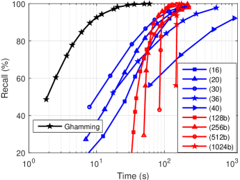
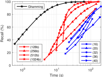
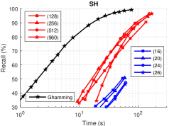
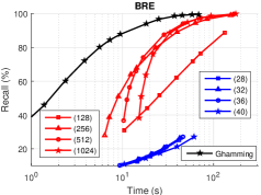
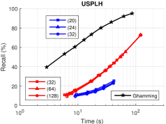
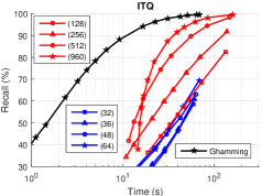
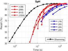
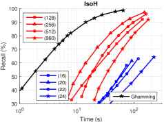
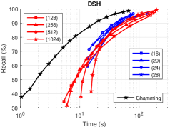
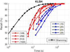
Generally speaking, the hash bucket search approach has the advantage on SIFT1M while the hamming ranking approach is preferred on GIST1M. For the hash bucket search approach, the optimal $m$ is 34 on SIFT1M and 28 on GIST1M. For the hamming ranking approach, longer code is preferred when we aim at a high recall while short code has the advantage when we aim at a low recall. It is important to note that these optimal parameters (the code length for the hamming ranking and table number for the hash bucket search) will change if we use another hashing algorithm (see Figure 10 and 11). A fair comparison between various hashing algorithms seems impossible.

(a) SIFT1M

(b) GIST1M

Figure 8: The recall - time curves of LSH with the hamming ranking and the hash bucket search approaches on SIFT1M and GIST1M. The read curves are the hamming ranking approach and the blue curves are the hash bucket search approach. The hamming ranking approach uses 128, 256, 512 and 1,024 bits and the hash bucket search approach use $\lceil\frac{1024}{w}\rceil$ tables to represent 1024 bits code, each table is $w$ bits, where table width $w$ is 16, 20, 30(32), 36 and 40.

(a) SIFT1M

(b) GIST1M

Figure 9: The recall-time curves of LSH with the grouped hamming ranking, the hamming ranking and the hash bucket search approaches on SIFT1M and GIST1M. The red and blue curves are the same as the curves in Figure 8. The black curve is the grouped hamming ranking approach proposed in this paper. The grouped hamming ranking approach is significant better than other two approaches on both datasets.

3 Grouped Hamming Ranking Approach

The commonly used approaches (the hamming ranking and the hash bucket search) for search with a hash index have their own pros and cons. Different hashing algorithms prefer different approach on different dataset (see Figure 10 and 11). It is not a easy task to fairly compare different hashing algorithms simply based on these two approaches. In this section, we are aiming at developing a better way to search with a hash index.

Algorithm 5 Grouped hamming ranking

1:base set D, query vector $q$, the hash functions, hash index (binary codes for all the points in the base set), kmeans partition of the base set, the nearest clusters $C$,the pool size $L$ and the number $K$ of required nearest neighbors,

2:$K$ points from the base set which are close to $q$.

3:Encode the query $q$ to a binary code $b$;

4:Find the $C$ nearest clusters to $q$

5:Compute the hamming distances between $b$ and all the binary codes in $C$ clusters;

6:Find the first $L$ points with shortest hamming distance to $b$;Grouped

7:return the closet $K$ points to $q$ among these $L$ points.

The proposed approach is based on the hamming ranking approach. Recall that the majority part of the locating time using the hamming ranking approach spends on the computation of the Hamming distances of the query code and all the database codes. If we can find an efficient wa to filter out those points which are unlikely to be the answers, we can reduce this computation.

Follow the the idea in [16], we use kmeans to group the samples into $k$ clusters at the indexing stage, and we represent each cluster with its centroid. At the on-line query stage, instead of computing the Hamming distances of the query code and the entire database codes, we can only focus on the nearest $c$ clusters (measured by the distance of the query vector and the centroid). We named this approach as Grouped Hamming Ranking.

To use grouped hamming ranking, besides the binary code, we need a kmeans partition of the database. The search procedure is summarized in Algorithm 5. There will be two parameters $C$ and $L$ which can be used to control the accuracy-efficiency trade-off.

Figure 10: The comparison of three search-the-hash-index approaches with 11 hashing algorithms on SIFT1M. The red curves are hamming ranking approaches with the numbers in the legend indicate the code length. The blue curves are hash bucket search approaches with the numbers in the legend indicates the table width. If the $w$ is the table width, the corresponding table number is $\lceil\frac{1024}{w}\rceil$. The black curve is the grouped hamming ranking approach proposed in this paper. No matter which hashing algorithm is used, the grouped hamming ranking approach is significant better than other two approaches.

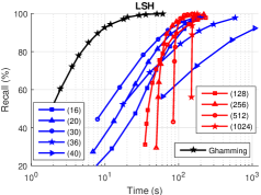
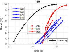
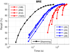
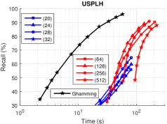
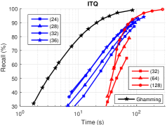
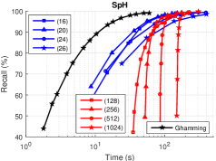
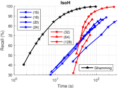
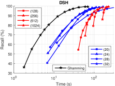
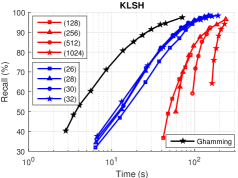
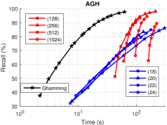
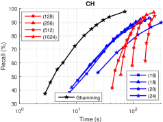
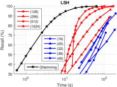
Figure 9 shows the performance of LSH on two datasets with the grouped hamming ranking approach (we generated 1,000 clusters with kmeans and 1,024 bits codes were used). The curve of grouped hamming ranking approach is added on the Figure 8 and we can see the significant advantage of the grouped hamming ranking approach over the other two commonly used approaches. Figure 10 and 11 show the performance of three search-the-hash-index approaches with 11 hashing algorithms on two datasets. The grouped hamming ranking approach outperforms the other two approaches for all the hashing algorithms on both two datasets.

Figure 11: The comparison of three search-the-hash-index approaches with 11 hashing algorithms on GIST1M. The red curves are hamming ranking approaches with the numbers in the legend indicate the code length. The blue curves are hash bucket search approaches with the numbers in the legend indicates the table width. If the $w$ is the table width, the corresponding table number is $\lceil\frac{1024}{w}\rceil$. The black curve is the grouped hamming ranking approach proposed in this paper. No matter which hashing algorithm is used, the grouped hamming ranking approach is significant better than other two approaches.

4 A Comprehensive Comparison

With the proposed grouped hamming ranking approach, we are ready to conduct a fair comparison between different hashing algorithms. In this Section, we will conduct a comprehensive comparison between eleven popular hashing algorithms on SIFT1M and GIST1M.

4.1 Compared Algorithms

Eleven popular hashing algorithms compared in the experiments are listed as follows:

• LSH is a short name for random-projection-based Locality Sensitive Hashing [5] as in Algorithm 2. It is frequently used as a baseline method in various hashing papers.

• SH is a short name for Spectral Hashing [41]. SH is based on quantizing the values of analytical eigenfunctions computed along PCA directions of the data.

• KLSH is a short name for Kernelized Locality Sensitive Hashing [25]. KLSH generalizes the LSH method to the kernel space.

• BRE is a short name for Binary Reconstructive Embeddings [24].

• USPLH is a short name for Unsupervised Sequential Projection Learning Hashing [37].

• ITQ is a short name for ITerative Quantization [11]. ITQ finds a rotation of zero-centered data so as to minimize the quantization error of mapping this data to the vertices of a zero-centered binary hypercube.

• AGH is a short name for Anchor Graph Hashing [31]. It aims at performing spectral analysis [2] of the data which shares the same goal with Self-taught Hashing [44]. The advantage of AGH over Self-taught Hashing is the computational efficiency. AGH uses an anchor graph [28] to speed up the spectral analysis.

  TABLE IV: Indexing Time (s)

  Method	SIFT1M	GIST1M	Method	SIFT1M	GIST1M
  LSH	3.35	12.33	SH	83.44	3864.3
  BRE	680.3	369.49	IsoH	1.68	91.99
  USPLH	1099.2	10508.3	KLSH	94.09	194.89
  ITQ	88.3	1372.4	AGH	296.84	389.91
  SpH	2583.5	4041.1	CH	263.78	365.34
  DSH	51.92	122.84
  ITQ, SH and IsoH learn 128 bits code on SIFT1M and 960 bits code
  on GIST1M.

  TABLE V: Coding Time (s)

  Method	SIFT1M	GIST1M	Method	SIFT1M	GIST1M
  LSH	0.03	0.016	SH	1.21	6.82
  BRE	0.25	0.043	IsoH	0.007	0.034
  USPLH	0.05	0.02	KLSH	0.34	0.06
  ITQ	0.01	0.025	AGH	0.86	0.11
  SpH	0.11	0.027	CH	0.96	0.10
  DSH	0.04	0.02
  ITQ, SH and IsoH use 128 bits code on SIFT1M and 960 bits code
  on GIST1M.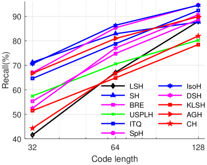

  

  

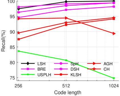
  Figure 12: The recall - codelength curves of various hashing algorithms when locate 10000 samples on SIFT1M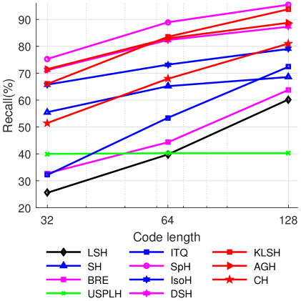

  

  

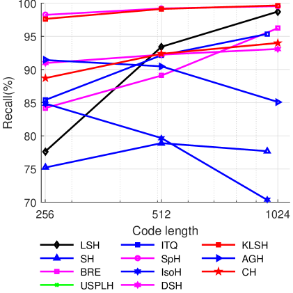
  Figure 13: The recall - codelength curves of various hashing algorithms when locate 50000 samples on GIST1M

• SpH is a short name for Spherical Hashing [14]. SpH uses a hyperspherebased hash function to map data points into binary codes.

• IsoH is a short name for Isotropic Hashing [23]. IsoH learns the projection functions with isotropic variances for PCA projected data. The main motivation of IsoH is that PCA directions with different variance should not be equally treated (one bit for one direction).

• CH is a short name for Compressed Hashing [27]. CH first learns a landmark (anchor) based sparse representation [6] then followed by LSH.

• DSH is a short name for Density Sensitive Hashing [18]. DSH finds the projections which aware the density distribution of the data.

For SH, ITQ, and IsoH, the learning process will involve the computation of eigenvectors of the covariance matrix. Thus, these three algorithms can only learn 128-bits code on SIFT1M and 960-bits code on GIST1M. All the other eight algorithms learn 1,024-bits code on both datasets.

For KLSH, AGH and CH, we need to pick a certain number of anchor (landmark) points. We use the same 1,500 anchor points for all these algorithms, and the anchor points are generated by using kmeans with five iterations. Also, the number of nearest anchors is set to 50 for AGH and CH algorithms. Please see [31] for details.

All the hashing algorithms are implemented in Matlab, and we use these hashing functions to learn the binary codes for both base vectors and query vectors. The binary codes can then be fed into Algorithm 5 for search. We use the same 1,000 clusters generated by kmeans for all the hashing algorithms. The Matlab functions are run on an i7-5930K CPU with 128G memory, and the Algorithm 5 is implemented in c++ and run on an i7-4790K CPU and 32G memory. For the sake of reproducibility, both the Matlab codes and c++ codes are released on GitHub.

Besides all the hashing algorithms, we also report the performance of the brute-force search as a baseline.

• brute-force. The performance of brute-force search is reported to show the advantages of using hashing methods. To get different recall, we simply perform brute-force search on different percentage of the query number. For example, the brute-force search time on 90% queries of the origin query set stands for the brute-force search time of 90% recall.

Figure 14: The recall-time curves of various hashing algorithms using the grouped hamming ranking approach on SIFT1M.

Figure 15: The recall-time curves of various hashing algorithms using the grouped hamming ranking approach on GIST1M.

Figure 16: The recall-time curves of various hashing algorithms using the grouped hamming ranking approach with $k=1$.

Figure 17: The recall-time curves of various hashing algorithms using the grouped hamming ranking approach with $k=10$.

4.2 Results

Since we use Matlab functions to learn the binary codes and c++ algorithm to search with a hash index, the coding time and later time (locating time and scanning time) cannot be added together, and we reported them separately.

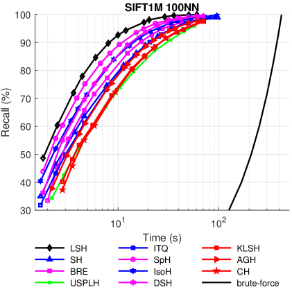
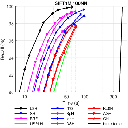
Table IV and V report the indexing (hash learning) time and coding (testing) time of various hashing algorithms. The indexing (hash learning) stage is performed off-line thus the indexing time is not very crucial. The coding time of all the hashing algorithms is short. Therefore the coding time can be ignored compared with locating time and scanning time (see Figure 14 and 15) when we consider the total search time.

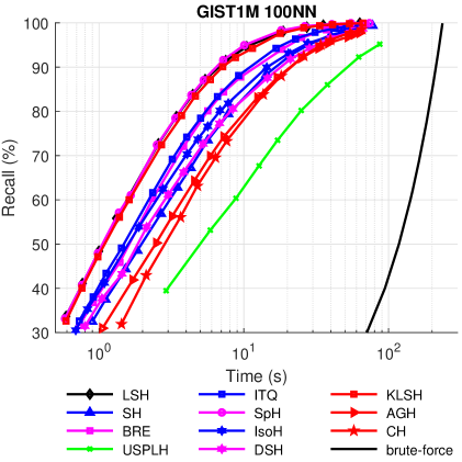
Figure 12 and 13 show how the recall changes as the code length increases of various hashing algorithms when the number of the located samples are fixed at 10,000 on SIFT1M and 50,000 on GIST1M. This figure illustrates several interesting points:

• When the code length is 32, all of the other algorithms outperform LSH on both two datasets. When the code length is 64, eight algorithms outperform LSH on SIFT1M, and nine algorithms outperform LSH on GIST1M. However, when the code length exceeds 512, LSH performs the best on SIFT1M and the 3rd best on GIST1M. This result is consistent with the finding in [20] that ”many data-dependent hashing algorithms have the improvements over LSH, but improvements occur only for relatively small hash code sizes up to 64 or 128 bits”. This result is also consistent with the ”outperform LSH” claim in all these hashing papers since they never report the performance using longer codes.

• If the locating time is ignored, the performance of most of the algorithms increases as the code length increases. However, on SIFT1M, the recall of USPLH decreases as the code length exceeds 256 and the recall of AGH decreases as the code length exceeds 512. On GIST1M, the recall of USPLH almost fixed as the code length increases and the recalls of AGH, SH and IsoH decrease as the code length exceeds 512. This result suggests the four hashing algorithms, USPLH, AGH, SH, and IsoH may not be able to learn very long discriminative codes.

We cannot judge which algorithm is better based merely on Figure 12 and 13, since the locating time is ignored. To pick the best hashing algorithm, we have to use the hashing code as the index and use time - recall curve to see the ANNS performance.

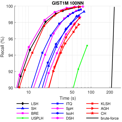
For all the hashing algorithms, we use the Algorithm 5 (the grouped hamming ranking approach) for search. All the algorithms use the same 1,000 clusters generated by kmeans. Based on the Figure 12 and 13, we can pick the optimal code length of each hash algorithm. On SIFT1M, SH, ITQ and IsoH use 128 bits code, AGH and USPLH use 256 bits code, and all the other hashing algorithms use 1,024 bits code. On GIST1M, AGH and IsoH use 256 bits code, ITQ uses 960 bits code, USPLH uses 64 bits code, and all the other hashing algorithms use 1,024 bits code.

Figure 18: The performance of LSH using the grouped hamming ranking approach with various cluster number.

Figure 19: The performance of LSH using the grouped hamming ranking approach with various code length.

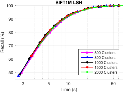
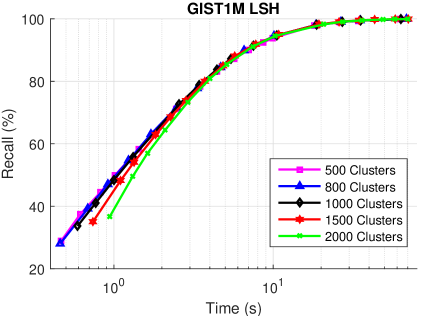
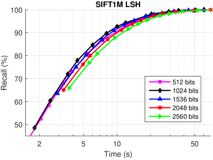
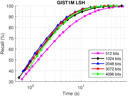
Figure 14 and 15 show the recall-time curves of various hashing algorithms using the grouped hamming ranking approach on SIFT1M and GIST1M respectively. A number of interesting points can be found: On SIFT1M, LSH performs significantly better than all the other hashing algorithms. On GIST1M, LSH is the second best-performed algorithm. It is slightly worse than SpH. Considering the extreme simplicity of LSH, we can conclude that LSH is the best choice among all the eleven compared hashing algorithms. This finding is a contradiction to the conclusions in most of the previous hashing papers.

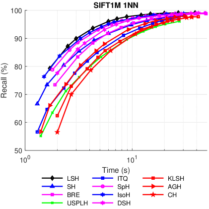
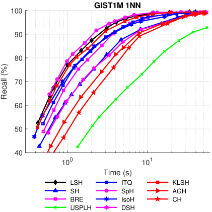
In the previous and the remaining experiments, we require all the algorithms to return 100 answers, i.e., fix $K=100$. To show this setting is reasonable, we plot the recall-time curves of various hashing algorithms with $K=1$ and $K=10$ in the Figure 16 and 17. We can see the same trend as $K=100$. As $K=1,10,100$, LSH is always the best performed algorithm on SIFT1M and the second best-performed algorithm on GIST1M.

4.3 Parameters of The Grouped Hamming Ranking

There are two essential parameters in the proposed grouped hamming ranking approach: the number of groups $G$ and the binary code length $l$. In this Section, we will discuss how these two parameters affect the performance of the grouped hamming ranking approach.

Figure 18 shows the performance of LSH on SIFT1M and GIST1M with various number of clusters (500, 800, 1,000, 1,500 and 2,000) using the grouped hamming ranking. We can see the search performance is very stable. With 1M points, 1,000 clusters means the average number of points in each cluster is 1,000. This is a reasonable choice.

The binary code length is another important parameter. In the previous experiment, we choose this parameter for various hashing algorithms based on the recall-codelength curve (See Figure 12 and 13). And we set the maximum length to be 1,024. It turns out that most of the compared hashing algorithms choose this parameter as 1,024. How about we further increase the code length? Figure 19 shows the performance of LSH on SIFT1M and GIST1M with various code length. On SIFT1M, LSH with grouped hamming ranking reaches the best search performance as the code length is 1,024. The search performance slowly decreases as the code length further increases. On GIST1M, the optimal code length becomes 2,048.

(a) SIFT1M

(b) GIST1M

Figure 20: The recall-time curves of six popular ANNS methods on SIFT1M and GIST1M.

5 Comparison with other popular ANNS methods

Given the surprising performance of random-projection-based LSH, we want to compare it with some public popular ANNS software. To be fair, we convert our Matlab code for random-projection-based LSH to c++ code and make a complete search software (by c++). We named our algorithm RPLSH. The codes are also released on GitHub.

5.1 Compared Algorithms

We pick five popular ANNS algorithms for comparison which cover various types such as tree-based, hashing-based, quantization-based and graph-based approaches. They are:

1. FALCONN is a well-known ANNS library based on multi-probe locality sensitive hashing. It implements the hash bucket search with multiple tables approach.

2. flann is a well-known ANNS library based on trees [34]. It integrates Randomized KD-tree [36] and Kmeans tree [8]. In our experiment, we use the randomized KD-tree and set the number of the trees as 32 on SIFT1M and 64 on GIST1M. The code on GitHub can be found at.

3. annoy is based on a binary search forest index. We use their code on GitHub for comparison.

4. faiss is recently released by Facebook. It contains well implemented code for state-of-the-art product quantization [16] based methods both on CPU and GPU. The CPU version is used for a fair comparison.

5. KGraph has open source code GitHub at, which is based on an approximate $k$NN Graph.

The experiments are carried out on a machine with an i7-4790k CPU and 32G memory. The performance on the high recall region for an ANNS algorithm will be more crucial in real applications. Thus we sample one percentage points from each base set as its corresponding validation set and tune all the algorithms on the validation sets to get their best-performing indices at the high recall region. For RPLSH, we use 1,024-bits code and 1,000 clusters. For all the search experiments, we only evaluate the algorithms on a single thread.

5.2 Results

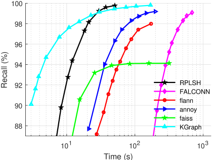
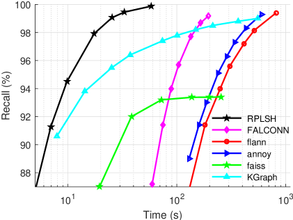
The recall-time curves of the six compared ANNS methods are shown in Figure 20. A number of interesting conclusions can be made:

• On both two datasets, RPLSH performs at least the second best among all the six compared algorithms when the recall is higher than 87%. On SIFT1M, If the recall is higher than 99% on SIFT1M and higher than 90% on GIST1M, RPLSH performs the best.

• Both the RPLSH and the FALCONN are LSH based algorithms. RPLSH significantly outperforms FALCONN on both two datasets. This probably dues to the reason that RPLSH uses the grouped hamming ranking approach while FALCONN uses the hash buckets search with multiple tables approach.

• flann and annoy are tree-based methods. Compare the performance of two hashing-based methods with that of two tree-based methods, and we can find that tree-based methods are more suitable for low dimensional data.

• faiss is a product quantization (PQ) [16] based method, and it uses binary codes to approximate the original features. Thus it is impossible for faiss to achieve a very high recall. The advantage of this approximation is that we do not need the original vectors which is a huge saving of the memory usage [16].

• KGraph is a graph-based algorithm, and it is KGraph’s author who says ”LSH is so hopelessly slow and/or inaccurate”. However, RPLSH is significantly better than KGraph on GIST1M when the recall is higher than 90%.

6 Conclusions

We carefully studied the problem of using hashing algorithms for ANNS. We introduce a novel approach (grouped hamming ranking) to search with a hash index. With this new approach, random-projection-based LSH is superior to many other popular hashing algorithms, and this algorithm is extremely simple. All the codes used in the paper are released on GitHub, which can be used as a testing platform for a fair comparison between various hashing methods.

References

- [1] S. Arya and D. M. Mount. Approximate nearest neighbor queries in fixed dimensions. In Proceedings of the Fourth Annual ACM/SIGACT-SIAM Symposium on Discrete Algorithms, 1993.
- [2] M. Belkin and P. Niyogi. Laplacian eigenmaps and spectral techniques for embedding and clustering. In Advances in Neural Information Processing Systems 14, 2001.
- [3] H. Ben and D. Tom. FANNG: Fast approximate nearest neighbour graphs. In Proceedings of the 2016 IEEE Conference on Computer Vision and Pattern Recognition, pages 5713–5722, 2016.
- [4] J. L. Bentley. Multidimensional binary search trees used for associative searching. Communications of the ACM, 18(9):509–517, 1975.
- [5] M. S. Charikar. Similarity estimation techniques from rounding algorithms. In Proceedings of the Thiry-fourth Annual ACM Symposium on Theory of Computing, pages 380–388, 2002.
- [6] X. Chen and D. Cai. Large scale spectral clustering with landmark-based representation. In Proceedings of the Twenty-Fifth AAAI Conference on Artificial Intelligence, 2011.
- [7] C. Fu, C. Xiang, C. Wang, and D. Cai. Fast approximate nearest neighbor search with the navigating spreading-out graphs. PVLDB, 12(5):461 – 474, 2019.
- [8] K. Fukunaga and P. M. Narendra. A branch and bound algorithm for computing k-nearest neighbors. IEEE Transactions on Computers, 100(7):750–753, 1975.
- [9] T. Ge, K. He, Q. Ke, and J. Sun. Optimized product quantization for approximate nearest neighbor search. In 2013 IEEE Conference on Computer Vision and Pattern Recognition, 2013.
- [10] A. Gionis, P. Indyk, and R. Motwani. Similarity search in high dimensions via hashing. In Proceedings of the 25th International Conference on Very Large Data Bases, 1999.
- [11] Y. Gong and S. Lazebnik. Iterative quantization: A procrustean approach to learning binary codes. In The 24th IEEE Conference on Computer Vision and Pattern Recognition, 2011.
- [12] J. He, W. Liu, and S. Chang. Scalable similarity search with optimized kernel hashing. In Proceedings of the 16th ACM International Conference on Knowledge Discovery and Data Mining, 2010.
- [13] K. He, F. Wen, and J. Sun. K-means hashing: An affinity-preserving quantization method for learning binary compact codes. In 2013 IEEE Conference on Computer Vision and Pattern Recognition, 2013.
- [14] J. Heo, Y. Lee, J. He, S. Chang, and S. Yoon. Spherical hashing. In 2012 IEEE Conference on Computer Vision and Pattern Recognition, 2012.
- [15] P. Indyk and R. Motwani. Approximate nearest neighbors: Towards removing the curse of dimensionality. In Proceedings of the Thirtieth Annual ACM Symposium on the Theory of Computing, 1998.
- [16] H. Jégou, M. Douze, and C. Schmid. Product quantization for nearest neighbor search. IEEE Trans. Pattern Anal. Mach. Intell., 33(1):117–128, 2011.
- [17] Z. Jin, Y. Hu, Y. Lin, D. Zhang, S. Lin, D. Cai, and X. Li. Complementary projection hashing. In IEEE International Conference on Computer Vision, 2013.
- [18] Z. Jin, C. Li, Y. Lin, and D. Cai. Density sensitive hashing. IEEE Trans. Cybernetics, 44(8):1362–1371, 2014.
- [19] Z. Jin, D. Zhang, Y. Hu, S. Lin, D. Cai, and X. He. Fast and accurate hashing via iterative nearest neighbors expansion. IEEE transactions on cybernetics, 44(11):2167–2177, 2014.
- [20] A. Joly and O. Buisson. Random maximum margin hashing. In The 24th IEEE Conference on Computer Vision and Pattern Recognition, 2011.
- [21] Y. Kalantidis and Y. S. Avrithis. Locally optimized product quantization for approximate nearest neighbor search. In 2014 IEEE Conference on Computer Vision and Pattern Recognition, 2014.
- [22] J. M. Kleinberg. Two algorithms for nearest-neighbor search in high dimensions. In Proceedings of the Twenty-Ninth Annual ACM Symposium on the Theory of Computing, 1997.
- [23] W. Kong and W. Li. Isotropic hashing. In Advances in Neural Information Processing Systems 25, 2012.
- [24] B. Kulis and T. Darrell. Learning to hash with binary reconstructive embeddings. In Advances in Neural Information Processing Systems 22, NIPS, 2009.
- [25] B. Kulis and K. Grauman. Kernelized locality-sensitive hashing for scalable image search. In IEEE 12th International Conference on Computer Vision, 2009.
- [26] W. Li, Y. Zhang, Y. Sun, W. Wang, W. Zhang, and X. Lin. Approximate nearest neighbor search on high dimensional data—experiments, analyses, and improvement (v1. 0). arXiv:1610.02455, 2016.
- [27] Y. Lin, R. Jin, D. Cai, S. Yan, and X. Li. Compressed hashing. In 2013 IEEE Conference on Computer Vision and Pattern Recognition, 2013.
- [28] W. Liu, J. He, and S.-F. Chang. Large graph construction for scalable semi-supervised learning. In Proceedings of the 27th International Conference on Machine Learning, 2010.
- [29] W. Liu, C. Mu, S. Kumar, and S. Chang. Discrete graph hashing. In Advances in Neural Information Processing Systems 27, 2014.
- [30] W. Liu, J. Wang, R. Ji, Y. Jiang, and S. Chang. Supervised hashing with kernels. In 2012 IEEE Conference on Computer Vision and Pattern Recognition, 2012.
- [31] W. Liu, J. Wang, S. Kumar, and S. Chang. Hashing with graphs. In Proceedings of the 28th International Conference on Machine Learning, 2011.
- [32] J. Makhoul, F. Kubala, R. Schwartz, and R. Weischedel. Performance measures for information extraction. In Proceedings of DARPA Broadcast News Workshop, 2000.
- [33] Y. A. Malkov and D. A. Yashunin. Efficient and robust approximate nearest neighbor search using hierarchical navigable small world graphs. arXiv:1603.09320, 2016.
- [34] M. Muja and D. G. Lowe. Scalable nearest neighbor algorithms for high dimensional data. IEEE Transactions on Pattern Analysis and Machine Intelligence, 36(11):2227–2240, 2014.
- [35] M. Norouzi and D. J. Fleet. Minimal loss hashing for compact binary codes. In Proceedings of the 28th International Conference on Machine Learning,ICML 2011, 2011.
- [36] C. Silpa-Anan and R. Hartley. Optimised kd-trees for fast image descriptor matching. In Proceedings of the 2008 IEEE Conference on Computer Vision and Pattern Recognition, 2008.
- [37] J. Wang, S. Kumar, and S. Chang. Sequential projection learning for hashing with compact codes. In Proceedings of the 27th International Conference on Machine Learning, 2010.
- [38] H. S. Warren. Hacker’s Delight, Chapter 5. Addison-Wesley Professional, 2012.
- [39] R. Weber, H.-J. Schek, and S. Blott. A quantitative analysis and performance study for similarity-search methods in high-dimensional spaces. In VLDB, 1998.
- [40] Y. Weiss, R. Fergus, and A. Torralba. Multidimensional spectral hashing. In 12th European Conference on Computer Vision, 2012.
- [41] Y. Weiss, A. Torralba, and R. Fergus. Spectral hashing. In Advances in Neural Information Processing Systems 21, NIPS, 2008.
- [42] B. Xu, J. Bu, Y. Lin, C. Chen, X. He, and D. Cai. Harmonious hashing. In Proceedings of the 23rd International Joint Conference on Artificial Intelligence, 2013.
- [43] H. Xu, J. Wang, Z. Li, G. Zeng, S. Li, and N. Yu. Complementary hashing for approximate nearest neighbor search. In IEEE International Conference on Computer Vision, 2011.
- [44] D. Zhang, J. Wang, D. Cai, and J. Lu. Self-taught hashing for fast similarity search. In Proceeding of the 33rd International ACM SIGIR Conference on Research and Development in Information Retrieval, 2010.