An efficient hybrid tridiagonal divide-and-conquer algorithm on distributed memory architectures

Abstract

In this paper, an efficient divide-and-conquer (DC) algorithm is proposed for the symmetric tridiagonal matrices based on ScaLAPACK and the hierarchically semiseparable (HSS) matrices. HSS is an important type of rank-structured matrices. Most time of the DC algorithm is cost by computing the eigenvectors via the matrix-matrix multiplications (MMM). In our parallel hybrid DC (PHDC) algorithm, MMM is accelerated by using the HSS matrix techniques when the intermediate matrix is large. All the HSS algorithms are done via the package STRUMPACK. PHDC has been tested by using many different matrices. Compared with the DC implementation in MKL, PHDC can be faster for some matrices with few deflations when using hundreds of processes. However, the gains decrease as the number of processes increases. The comparisons of PHDC with ELPA (the Eigenvalue soLvers for Petascale Applications library) are similar. PHDC is usually slower than MKL and ELPA when using 300 or more processes on Tianhe-2 supercomputer.

1 Introduction

The symmetric tridiagonal eigenvalue problems are usually solved by the divide and conquer (DC) algorithm both on shared memory multicore platforms and parallel distributed memory machines. The DC algorithm is fast and stable, and well-studied in numerous references [13, 4, 25, 18, 15, 38]. It is now the default method in LAPACK [1] and ScaLAPACK [12] when the eigenvectors of a symmetric tridiagonal matrix are required.

Recently, the authors [27] used the hierarchically semiseparable (HSS) matrices [8] to accelerate the tridiagonal DC in LAPACK, and obtained about 6x speedups in comparison with that in LAPACK for some large matrices on a shared memory multicore platform. The bidiagonal and banded DC algorithms for the SVD problem are accelerated similarly [26, 28]. The main point is that some intermediate eigenvector matrices are rank-structured matrices [8, 20]. The HSS matrices are used to approximate them and then use fast HSS algorithms to update the eigenvectors. HSS is an important type of rank-structured matrices, and others include $\mathcal{H}$-matrix [20], $\mathcal{H}^{2}$-matrix [22], quasiseparable [14] and sequentially semiseparable (SSS) [7, 19]. In this paper, we extend the techniques used in [26, 27] to the distributed memory environment, try to accelerate the tridiagonal DC algorithm in ScaLAPACK [12]. To integrate HSS algorithms into ScaLAPACK routines, an efficient distributed HSS construction routine and an HSS matrix multiplication routine are required. In our experiments, we use the routines in STRUMPACK (STRUctured Matrices PACKage) package [36], which is designed for computations with both sparse and dense structured matrices. The current STRUMPACK has two main components: dense matrix computation package and sparse direct solver and preconditioner. In this work we only use its dense matrix operation part. It is written in C++ using OpenMP and MPI parallism, uses HSS matrices, and it implements a parallel HSS construction algorithm with randomized sampling [35, 24]. Note that some routines are available for sequential HSS algorithms [43, 10] or parallel HSS algorithms on shared memory platforms such as HSSPACK [28]. But STRUMPACK is the only available one for the distributed parallel HSS algorithms. More details about it and HSS matrices will be introduced in section 2.

The ScaLAPACK routine implements the rank-one update of Cuppen’s DC algorithm [13]. We briefly introduce the main processes. Assume that $T$ is a symmetric tridiagonal matrix,

$$T=\begin{pmatrix}a_{1}&b_{1}&&\\ b_{1}&\ddots&\ddots&\\ &\ddots&a_{N-1}&b_{N-1}\\ &&b_{N-1}&a_{N}\end{pmatrix}.$$ (1)

Cuppen introduced the decomposition

$$T=\begin{pmatrix}T_{1}&\\ &T_{2}\end{pmatrix}+b_{k}vv^{T},$$ (2)

where $T_{1}\in R^{k\times k}$ and $v=[0,\ldots,0,1,1,0,\ldots,0]^{T}$ with ones at the $k$-th and $(k+1)$-th entries. Let $T_{1}=Q_{1}D_{1}Q_{1}^{T}$ be $T_{2}=Q_{2}D_{2}Q_{2}^{T}$ be eigen decompositions, and then (1) can be written as

$$T=Q\left(D+b_{k}zz^{T}\right)Q^{T},$$ (3)

where $Q=\text{diag}(Q_{1},Q_{2})$, $D=\text{diag}(D_{1},D_{2})$ and $z=Q^{T}v=\begin{pmatrix}\text{last column of }Q_{1}^{T}\\ \text{first column of }Q_{2}^{T}\end{pmatrix}.$ The problem is reduced to computing the spectral decomposition of the diagonal plus rank-one

$$D+b_{k}uu^{T}=\widehat{Q}\Lambda\widehat{Q}^{T}.$$ (4)

By Theorem 2.1 in [13], the eigenvalues $\lambda_{i}$ of matrix $D+b_{k}zz^{T}$ are the root of the secular equation

$$f(\lambda)=1+b_{k}\frac{z_{k}^{2}}{d_{k}-\lambda}=0,$$

where $z_{k}$ and $d_{k}$ are the $k$th component of $z$ and the kth diagonal entry of $D$, respectively, and its corresponding eigenvector is given by $\hat{q}_{i}=(D-\lambda_{i})^{-1}z.$ The eigenvectors simply computed this way may loss orthogonality. To ensure orthogonality, Sorensen and Tang [37] proposed to use extended precision. While, the implementation in ScaLAPACK uses the Löwner theorem approach, instead of the extended precision approach [37]. The extra precision approach was used by Gates and Arbenz [15] in their implementation.

Remark 1. The extra precision approach is “embarrassingly” parallel with each eigenvalue and eigenvector computed without communication, but it is not portable in some platform. The Löwner approach requires information about all the eigenvalues, requiring a broadcast. However, the length of communication message is $O(n)$ which is trivial compared with the $O(n^{2})$ communication of eigenvectors.

The excellent performance of the DC algorithm is partially due to deflation [4, 13], which happens in two cases. If the entry $z_{i}$ of $z$ are negligible or zero, the corresponding $(\lambda_{i},\hat{q}_{i})$ is already an eigenpair of $T$. Similarly, if two eigenvalues in $D$ are identical then one entry of $z$ can be transformed to zero by applying a sequence of plane rotations. All the deflated eigenvalues would be permuted to back of $D$ by a permutation matrix, so do the corresponding eigenvectors. Then (3) reduces to, after deflation,

$$T=Q(GP)\begin{pmatrix}\bar{D}+b_{k}\bar{z}\bar{z}^{T}&\\ &\bar{D}_{d}\end{pmatrix}(GP)^{T}Q^{T},$$ (5)

where $G$ is the product of all rotations, and $P$ is a permutation matrix and $\bar{D}_{d}$ are the deflated eigenvalues.

According to (4), the eigenvectors of $T$ are computed as

$$U=Q(GP)\begin{pmatrix}\widehat{Q}&\\ &I_{d}\end{pmatrix}=\left[\begin{pmatrix}Q_{1}&\\ &Q_{2}\end{pmatrix}GP\right]\begin{pmatrix}\widehat{Q}&\\ &I_{d}\end{pmatrix}.$$ (6)

To improve efficiency, Gu [17] suggested a permutation strategy for reorganizing the data structure of the orthogonal matrices, which has been used in ScaLAPACK. The matrix in square brackets is permuted as $\begin{pmatrix}{Q}_{11}&{Q}_{12}&0&{Q}_{14}\\ 0&{Q}_{22}&{Q}_{23}&{Q}_{24}\end{pmatrix}$, where the first and third block columns contain the eigenvectors that have not been affected by deflation, the fourth block column contains the deflated eigenvectors, and the second block column contains the remaining columns. Then, the computation of $U$ can be done by two parallel matrix-matrix products (calling PBLAS PDGEMM) involving parts of $\widehat{Q}$ and the matrices $\begin{pmatrix}Q_{11}&Q_{12}\end{pmatrix}$, $\begin{pmatrix}Q_{22}&Q_{23}\end{pmatrix}$. Another factor that contributes to the excellent performance of DC is that most operations can take advantage of highly optimized matrix-matrix products.

When there are few deflations, the size of matrix $\widehat{Q}$ in (6) will be large, and most time of DC would be cost by the matrix-matrix multiplication in (6), which is confirmed by the results of Example 2 in section 2.2. Furthermore, it is well-known that matrix $\widehat{Q}$ defined as in (4) is a Cauchy-like matrix with off-diagonally low rank property, see [18, 27]. Therefore, we simply use an HSS matrix to approximate $\widehat{Q}$ and use HSS matrix-matrix multiplication routine in STRUMPACK to compute the eigenvector matrix $U$ in (6). Since HSS matrix multiplications require much fewer floating point operations than the plain matrix-matrix multiplication, PDGEMM, this approach makes the DC algorithm in ScaLAPACK much faster. More details are included section 2.2 and numerical results are shown in section 3.

2 HSS matrices and STRUMPACK

The HSS matrix is an important type of rank-structured matrices. A matrix is called rank-structured if the ranks of all off-diagonal blocks are relatively small compared to the size of matrix. Other rank-structured matrices include $\mathcal{H}$-matrix [20, 23], $\mathcal{H}^{2}$-matrix [22, 21], quasiseparable matrices [14, 40], and sequentially semiseparable (SSS) [5, 6] matrices. We mostly follow the notation used in [35] and [41, 27] to introduce HSS.

Both HSS representations and algorithms rely on a tree $\mathcal{T}$. For simplicity, we assume it is a binary tree, name it HSS tree, and the generalization is straightforward. Assume that $\mathcal{I}=\{1,2,\ldots,N\}$ and $N$ is the dimension of matrix $A$. Each node $i$ of $\mathcal{T}$ is associated with a contiguous subset of $\mathcal{I}$, $t_{i}$, satisfying the following conditions:

• $t_{i_{1}}\cup t_{i_{2}}=t_{i}$ and $t_{i_{1}}\cap t_{i_{2}}=\emptyset$, for a parent node $i$ with left child $i_{1}$ and right child $i_{2}$;

• $\cup_{i\in LN}t_{i}=\mathcal{I}$, where $LN$ denotes the set of all leaf nodes;

• $t_{\operatorname*{root}(\mathcal{T})}=\mathcal{I}$, $\operatorname*{root}(\mathcal{T})$ denotes the root of $\mathcal{T}$.

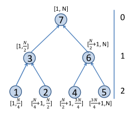
We assume $\mathcal{T}$ is postordered. That means the ordering of a nonleaf node $i$ satisfies $i_{1}<i_{2}<i$, where $i_{1}$ is its left child and $i_{2}$ is its right child. Figure 1(a) shows an HSS tree with three levels and $t_{i}$ associated with each node $i$.

(a) Matrix $A$

(b) HSS tree

Figure 1: A three level postordering tree $\mathcal{T}$ and the HSS blocks of Node 2

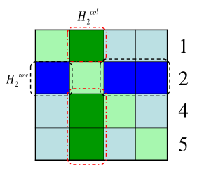
A block row or column excluding the diagonal block is called an HSS block row or column, denoted by

$$H_{i}^{row}=A_{t_{i}\times(\mathcal{I}\backslash t_{i})},\quad H_{i}^{col}=A_{(\mathcal{I}\backslash t_{i})\times t_{i}},$$

associated with node $i$. We simply call them HSS blocks. For an HSS matrix, HSS blocks are assumed to be numerically low-rank. Figure 1(b) shows the HSS blocks corresponding to node 2. We name the maximum (numerical) rank of all the HSS blocks by HSS rank.

For each node $i$ in $\mathcal{T}$, it associates with four generators $\widehat{D}_{i}$, $\widehat{U}_{i}$, $\widehat{V}_{i}$ and $B_{i}$, which are matrices, such that

$$\begin{split}\widehat{D}_{i}&=A|_{t_{i}\times t_{i}}=\begin{bmatrix}\widehat{D}_{i_{1}}&\widehat{U}_{i_{1}}B_{i_{1}}\widehat{V}_{i_{2}}^{T}\\ \widehat{U}_{i_{2}}B_{i_{2}}\widehat{V}_{i_{1}}^{T}&\widehat{D}_{i_{2}}\end{bmatrix},\\ \widehat{U}_{i}&=\begin{bmatrix}\widehat{U}_{i_{1}}&\\ &\widehat{U}_{i_{2}}\end{bmatrix}U_{i},\quad\widehat{V}_{i}=\begin{bmatrix}\widehat{V}_{i_{1}}&\\ &\widehat{V}_{i_{2}}\end{bmatrix}V_{i}.\end{split}$$ (7)

For a leaf node $i$, $\widehat{D}_{i}=D_{i}$, $\widehat{U}_{i}=U_{i}$, $\widehat{V}_{i}=V_{i}$. A $4\times 4$ (block) HSS matrix $A$ can be written as

$$A=\begin{bmatrix}\begin{bmatrix}D_{1}&{U}_{1}B_{1}{V}_{2}^{T}\\ {U}_{2}B_{2}{V}_{1}^{T}&D_{2}\end{bmatrix}&\widehat{U}_{3}B_{3}\widehat{V}_{6}^{T}\\ \widehat{U}_{6}B_{6}\widehat{V}_{3}^{T}&\begin{bmatrix}D_{4}&{U}_{4}B_{4}{V}_{5}^{T}\\ {U}_{5}B_{5}{V}_{4}^{T}&D_{5}\end{bmatrix}\end{bmatrix},$$ (8)

and Figure 1(a) shows its corresponding postordering HSS tree. The HSS representation (7) is equivalent to the representations in [36, 9, 8, 42].

To take advantage of the fast HSS algorithms, we need to construct an HSS matrix first. There exist many HSS construction algorithms such as using SVD [9], RRQR(rank revealing QR) [41], and so on. Most of these algorithms cost in $O(N^{2}r)$ flops, where $N$ is the dimension of matrix and $r$ is its HSS rank. In [35], a randomized HSS construction algorithm (RandHSS) is proposed, which combines random sampling with interpolative decomposition (ID), see [11, 24, 30]. The cost of RandHSS can be reduced to $O(Nr)$ flops if there exists a fast matrix-vector multiplication algorithm in order of $O(N)$ flops. STRUMPACK also uses this algorithm to construct HSS matrices. For completeness, RandHSS is restated in Algorithm 1.

Algorithm 1.  (Randomized HSS construction algorithm) Given a matrix $A$ and integers $r$ and $p$, generate two $N\times(r+p)$ Gaussian random matrices $\Omega^{(1)}$ and $\Omega^{(2)}$, and then compute matrices $Y=A\Omega^{(1)}$ and $Z=A^{T}\Omega^{(2)}$.

do $\ell=L,\cdots,1$

 

for node $i$ at level $\ell$

  

if $i$ is a leaf node,

1. $D_{i}=A_{t_{i},t_{i}}$;

2. compute $\Phi_{i}=Y_{i}-D_{i}\Omega_{i}^{(1)}$, $\Theta_{i}=Z_{i}-D_{i}^{T}\Omega_{i}^{(2)}$;

3. compute the ID of $\Phi_{i}\approx U_{i}\Phi_{i}|_{\tilde{I}_{i}}$, $\Theta_{i}\approx V_{i}\Theta_{i}|_{\tilde{J}_{i}}$;

4. compute $\widehat{Y}_{i}=V_{i}^{T}\Omega_{i}^{(1)}$, $\widehat{Z}_{i}=U_{i}^{T}\Omega_{i}^{(2)}$;

  

else

1. store generators $B_{i_{1}}=A(\tilde{I}_{i_{1}},\tilde{J}_{i_{2}})$, $B_{i_{2}}=A(\tilde{I}_{i_{2}},\tilde{J}_{i_{1}})$;

2. compute $\Phi_{i}=\begin{bmatrix}\Phi_{i_{1}}|_{\tilde{I}_{i_{1}}}-B_{i_{1}}\widehat{Y}_{i_{2}}\\ \Phi_{i_{2}}|_{\tilde{I}_{i_{2}}}-B_{i_{2}}\widehat{Y}_{i_{1}}\end{bmatrix}$,  $\Theta_{i}=\begin{bmatrix}\Theta_{i_{1}}|_{\tilde{J}_{i_{1}}}-B_{i_{2}}^{T}\widehat{Z}_{i_{2}}\\ \Theta_{i_{2}}|_{\tilde{J}_{i_{2}}}-B_{i_{1}}^{T}\widehat{Z}_{i_{1}}\end{bmatrix}$;

3. compute the ID of $\Phi_{i}\approx U_{i}\Phi_{i}|_{\tilde{I}_{i}}$,  $\Theta_{i}\approx V_{i}\Theta_{i}|_{\tilde{J}_{i}}$;

4. Compute $\widehat{Y}_{i}=V_{i}^{T}\begin{bmatrix}\widehat{Y}_{i_{1}}\\ \widehat{Y}_{i_{2}}\end{bmatrix}$,  $\widehat{Z}_{i}=U_{i}^{T}\begin{bmatrix}\widehat{Z}_{i_{1}}\\ \widehat{Z}_{i_{2}}\end{bmatrix}$;

  

end if

 

end for

end do

For the root node $i$, store $B_{i_{1}}=A(\tilde{I}_{i_{1}},\tilde{J}_{i_{2}})$, $B_{i_{2}}=A(\tilde{I}_{i_{2}},\tilde{J}_{i_{1}})$.

The parameter $r$ in Algorithm 1 is an estimate of the HSS rank of $A$, which would be chosen adaptively in STRUMPACK [36], and $p$ is the oversampling parameter, usually equals to $10$ or $20$, see [24]. After matrix $A$ is represented in its HSS form, there exist fast algorithms for multiplying it with a vector in $O(Nr)$ flops [32, 5]. Therefore, multiplying an HSS matrix with another $N\times N$ matrix only costs in $O(N^{2}r)$ flops. Note that the general matrix-matrix multiplication algorithm PDGEMM costs in $O(N^{3})$ flops.

2.1 STRUMPACK

STRUMPACK is an abbreviation of STRUctured Matrices PACKage, designed for computations with sparse and dense structured matrices. It is based on some parallel HSS algorithms using randomization [36, 16].

Comparing with ScaLAPACK, STRUMPACK requires more memory, since besides the original matrix it also stores the random vectors and the samples, and the generators of HSS matrix. The memory overhead increases as the HSS rank increases. Therefore, STRUMPACK is suitable for matrices with low off-diagonal ranks. For the our eigenvalue problems, we are fortunate that the HSS rank of intermediate eigenvector matrices appeared in the DC algorithm is not large, usually less than 100. Through the experiments in section 3, we let the compression threshold of constructing HSS be $1.0e$-$14$, to keep the orthogonality of computed eigenvectors. One advantage of STRUMPACK is that it requires much fewer operations than the classical algorithms by exploiting the off-diagonally low rank property.

Another property of STRUMPACAK, the same as other packages that explores low-rank structures ($\mathcal{H}$-matrices [3] and Block Low-Rank representations), is irregular computational patterns, dealing with irregular and imbalanced taskflows and manipulating a collection of small matrices instead of one large one. HSS algorithms requires a lower asymptotic complexity, but the flop rate with HSS is often lower than with traditional matrix-matrix multiplications, BLAS3 kernels. We expect HSS algorithms to have good performances for problems with large size. Therefore, we only use HSS algorithms when the problem size is large enough, just as in [26, 27].

The HSS construction algorithm in STRUMPACK uses randomized sampling algorithm combined with Interpolative Decomposition (ID) [30, 11], first proposed in [35]. For this randomized algorithm, the HSS rank needs to be estimated in advance, which is difficult to be estimated accurately. An adaptive sampling mechanism is proposed in STRUMPACK, and its basic idea [36] is ‘to start with a low number of random vectors $d$, and whenever the rank found during Interpolative Decomposition is too large, $d$ is increased’. To control the communication cost, we use a little more sample vectors ($p=100$) and let inc_rand_HSS relatively large which is a parameter for constructing HSS matrix in STRUMPACK.

In this work, we mainly use two STRUMPACK driver routines: the parallel HSS construction and parallel HSS matrix multiplication routines. We use these two routines to replace the general matrix-matrix multiplication routine PDGEMM in hope of achieving good speedups for large matrices. We test the efficiency and scalability of STRUMPACK by using an HSS matrix firstly appeared in the test routine of STRUMPACK [36].

Example 1. We use two $n\times n$ Toeplitz matrices, which have been used in [36]. In this example we assume $n=20,000$. The first one is defined as $a_{i,i}=n^{2}$ and $a_{i,j}=i-j$ for $i\neq j$, which is diagonally dominant and yields very low HSS rank (about 2). The second one is defined as $a_{i,i}=\frac{\pi^{2}}{6d^{2}}$ and $a_{i,j}=\frac{(-1)^{i-j}}{(i-j)^{2}d^{2}}$, which is a kinetic energy matrix from quantum chemistry [36], $d=0.1$ is a discretization parameter. This matrix has slightly larger HSS rank (about $160$).

Table 1: The comparisons of HSS matrix multiplication with PDGEMM

		$4$	$16$	$64$	$121$	$256$	$676$
PDGEMM		185.33	53.58	13.42	8.02	3.79	1.89
Mat1	Const	6.18	2.39	1.21	1.24	1.29	2.89
	Multi	16.64	11.65	3.72	2.46	1.78	1.75
	Speedup	8.12	3.82	2.72	2.17	1.23	0.41
Mat2	Const	4.57	1.80	0.96	1.20	1.23	2.68
	Multi	15.42	11.10	3.46	2.29	1.71	1.58
	Speedup	9.27	4.15	3.04	2.30	1.29	0.44

From the results in Table 1, the HSS matrix multiplication implemented in STRUMPACK can be more than 1.2x times faster than PDGEMM when the used processes are around 256. The speedups are even better when using fewer processes. But, the HSS construction and matrix multiplication algorithms are not as scalable as PDGEMM, and they become slower than PDGEMM when using more processes, for example more than 676. Therefore, it suggests to use no more than 256 processes when combining STRUMPACK with ScaLAPACK. The execution time highly depends on many factors, such as parameters NB, block_HSS, etc. The results in Table 1 were obtained by choosing $NB=64$ and $block\_HSS=512$. Note that we did not try to find the optimal parameters.

2.2 Combining DC with HSS

In this section we show more details of combining HSS matrix techniques with ScaLAPACK. As mentioned before, the central idea is to replace PDGEMM by the HSS matrix multiplication algorithms. The eigenvectors are updated in the ScaLAPACK routine PDLAED1, and therefore we modify it and call STRUMPACK routines in it instead of PDGEMM.

Note that after applying permutations to $Q$ in (6), matrix $\widehat{Q}$ should also be permuted accordingly. From the results in [18, 27, 26], we know that $\widehat{Q}$ is a Cauchy-like matrix and off-diagonally low-rank, the numerical rank is usually around $50$-$100$. When combining with HSS, we would not use Gu’s idea since permutation may destroy the off-diagonally low-rank structure of $\widehat{Q}$ in (6). We need to modify the ScaLAPACK routine PDLAED2, and only when the size of deflated matrix $\bar{D}$ in (5) is large enough, HSS techniques are used, otherwise use Gu’s idea. Denote the size of $\bar{D}$ by $K$, and it depends the architecture of particular parallel computers, and may be different for different computers.

Most work of DC is spent on the first two top-levels matrix-matrix multiplications. The first top-level takes nearly 50% when using 256 processes or fewer, see the results in Table 2 and also the results in [2]. Therefore, we could expect at most 2x speedup when replacing PDGEMM with parallel HSS matrix multiplications.

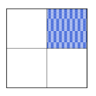
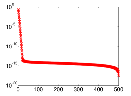
In this subsection, we fist use an example to show the off-diagonally low-rank property of $\widehat{Q}$ in (4). Here we assume that the dimension of $D$ is $N=1000$, and the diagonal entries of $D$ satisfy $d_{i}=\frac{i}{N}$, $i=1,\ldots,N$, $b_{k}=1$ and $u$ is a normalized random vector in (4). Then the singular values of matrix $\widehat{Q}(1:m,m+1:N)$ are illustrated in Figure 2(b) with $m=500$. From it, we get that the singular values decay very quickly.

(a) Matrix $\widehat{Q}$

(b) Singular values of $\widehat{Q}(1:m,m+1:N)$

Figure 2: The off-diagonally low-rank property of $\widehat{Q}$

Example 2. We use a symmetric tridiagonal matrix to show the percentage of time cost by the top level matrix-matrix multiplications. The diagonal entries of tridiagonal matrix $A$ are all two and its off-diagonal entries are all one. The size of this matrix is $n=20,000$.

Table 2: The percentage of time cost by the first top-level matrix-matrix multiplications

	$4$	$16$	$36$	$64$	$121$	$256$	$576$	$1024$
Top One	59.80	44.13	30.29	16.92	9.23	4.77	1.09	0.53
Total	108.04	77.06	52.78	30.04	17.70	10.00	6.20	6.22
Percent(%)	55.35	57.2	57.39	56.32	52.15	47.70	17.58	8.52

The results in Table 2 are obtained by using optimization flags "-O2 -C -qopenmp -mavx", and linked with multi-threaded Intel MKL. From the results in it, we can see that the top-one level matrix-matrix multiplications can take half of the total time cost by PDSTEDC in some case. Since PDGEMM in MKL has very good scalability, the percentage of top-one level matrix multiplications decreases as the number of processes increases. This example also implies that we are better not to use more than 256 processes in our numerical experiments.

3 Numerical results

All the results are obtained on Tianhe-2 supercomputer [29, 31], located in Guangzhou, China. It employs accelerator based architectures and each compute node is equipped with two Intel Xeon E5-2692 CPUs and three Intel Xeon Phi accelerators based on the many-integrated-core (MIC) architectures. In our experiments we only use CPU cores.

Example 3. We use some ‘difficult’ matrices [34] for the DC algorithm, for which few or no eigenvalues are deflated. Examples include the Clement-type, Hermite-type and Toeplitz-type matrices, which are defined as follows.

The Clement-type matrix [34] is given by

$$T=\text{tridiag}\begin{pmatrix}&\sqrt{n}&&\sqrt{2(n-1)}&&\sqrt{(n-1)2}&&\sqrt{n}&\\ 0&&0&&\ldots&&0&&0\\ &\sqrt{n}&&\sqrt{2(n-1)}&&\sqrt{(n-1)2}&&\sqrt{n}&\\ \end{pmatrix},$$ (9)

where the off-diagonal entries are $\sqrt{i(n+1-i)},i=1,\ldots,n$.

The Hermite-type matrix is given as [34],

$$T=\text{tridiag}\begin{pmatrix}&\sqrt{1}&&\sqrt{2}&&\sqrt{n-2}&&\sqrt{n-1}&\\ 0&&0&&\ldots&&0&&0\\ &\sqrt{1}&&\sqrt{2}&&\sqrt{n-2}&&\sqrt{n-1}&\\ \end{pmatrix}.$$ (10)

The Toeplitz-type matrix is defined as [34],

$$T=\text{tridiag}\begin{pmatrix}&1&&1&&1&&1&\\ 2&&2&&\ldots&&2&&2\\ &1&&2&&1&&1&\\ \end{pmatrix}.$$ (11)

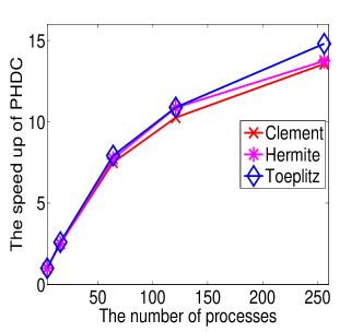
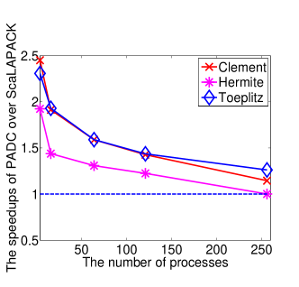
For the results of strong scaling, we let the dimension be $n$=$30,000$, and use HSS techniques only when the size of secular equation is larger than $K=20,000$. The results for strong scaling are shown in Figure 3(a). The speedups of PHDC over ScaLAPACK are reported in Table 3, and shown in Figure 3(b). We can see that PHDC is about $1.4$ times faster than PDSTEDC in MKL when using 120 processes or fewer.

Table 3: The strong scaling of PHDC compared with Intel MKL

Matrix	Number of Processes
	$4$	$16$	$64$	$121$	$256$
Clement	2.45	1.91	1.58	1.42	1.14
Hermite	1.92	1.43	1.30	1.22	1.00
Toeplitz	2.30	1.92	1.58	1.43	1.26

(a) The strong scaling of PHDC

(b) The speedups of PHDC over ScaLAPACK

Figure 3: The results for the difficult matrices

The orthogonality of the computed eigenvectors by PHDC are in the same order as those by ScaLAPACK, which are shown in Table 4. The orthogonality of matrix $Q$ is defined as $\|I-QQ^{T}\|_{\max}$, where $\|\bullet\|_{\max}$ is the maximum absolute value of entries of $(\bullet)$.

Table 4: The orthogonality of the computed eigenvectors by PHDC

Matrix	Number of Processes
	$4$	$16$	$64$	$121$	$256$
Clement	$1.6e$-$13$	$1.6e$-$13$	$1.6e$-$13$	$1.6e$-$13$	$1.6e$-$13$
Hermite	$3.6e$-$13$	$3.6e$-$13$	$3.6e$-$13$	$3.6e$-$13$	$3.6e$-$13$
Toeplitz	$2.9e$-$13$	$2.9e$-$13$	$2.9e$-$13$	$2.9e$-$13$	$2.9e$-$13$

Example 4. In [39], Tygert shows that the spherical harmonic transform (SHT) can be accelerated using the tridiagonal DC algorithm and one symmetric tridiagonal matrix is defined as follows,

$$A_{jk}=\begin{cases}c_{m+2j-2},&k=j-1\\ d_{m+2j},&k=j\\ c_{m+2j},&k=j+1\\ 0,&otherwise,\end{cases}$$ (12)

for $j,k=0,1,\ldots,n-1$, where

$$c_{l}=\sqrt{\frac{(l-m+1)(l-m+2)(l+m+1)(l+m+2)}{(2l+1)(2l+3)^{2}(2l+5)}},\quad d_{l}=\frac{2l(l+1)-2m^{2}-1}{(2l-1)(2l+3)},$$

for $l=m,m+1,m+2,\ldots.$ Assume that the dimension of this matrix is $n=30,000$ and $m=n$. The execution times of using PHDC and PDSTEDC are reported in Table 5.

Table 5: The execution time of PHDC and PDSTEDC for SHT

Method	Number of Processes
	$4$	$16$	$64$	$121$	$256$
PDSTEDC	475.00	139.09	39.66	25.82	16.87
PHDC	224.97	88.58	28.53	20.12	14.71
Speedup	2.11	1.57	1.39	1.28	1.15

3.1 Comparison with other implementations

Different from ScaLAPACK, the ELPA routines [2, 33] do not rely on BLACS, all communication between different processors is handled by direct calls to a MPI library, where ELPA stands for Eigenvalue soLver for Petascale Applications. For its communications, ELPA relies on two separate sets of MPI communicators, row communicators and column communicators, respectively (connecting either the processors that handle the same rows or the same columns). For the tridiagonal eigensolver, ELPA implements its own matrix-matrix multiplications, does not use PBLAS routine PDGEMM. It is known that ELPA has better scalability and is faster than MKL [2, 33].

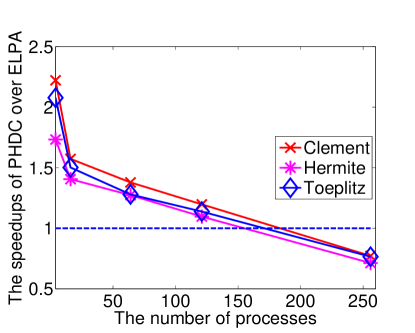
Example 5. We use the same matrices as in Example 3 to test ELPA, and compare it with the newly proposed algorithm PHDC. The running times of ELPA are shown in Table 6. Figure 4 shows the speedups of PHDC over ELPA. PHDC is faster than ELPA since it requires fewer floating point operations. However, its scalability is worse than ELPA, and PHDC becomes slower than ELPA when using more than 200 processes.

Table 6: The execution time of ELPA for different matrices

Matrix	Number of Processes
	$4$	$16$	$64$	$121$	$256$
Clement	487.63	137.43	40.36	25.61	12.49
Hermite	363.94	117.61	34.58	21.18	10.89
Toeplitz	509.32	141.57	39.55	25.62	12.67

Figure 4: The speedups of PHDC over ELPA for the difficult matrices

4 Conclusions

By combining ScaLAPACK with STRUMPACK, we propose a hybrid tridiagonal DC algorithm for the symmetric eigenvalue problems, which can be faster than the classical DC algorithm implemented in ScaLAPACK when using about 200 processes. The central idea is to relpace PDGEMM by the HSS matrix multiplication algorithms, since HSS matrix algorithms require fewer flops than PDGEMM. Numerical results show that the scalability of HSS matrix algorithms is not as good as PDGEMM. The proposed PHDC algorithm in this work becomes slower than the classical DC algorithm when using more processes.

References

- [1] E. Anderson, Z. Bai, C. Bischof, S. Blackford, J. Demmel, J. Dongarra, J. Du Croz, A. Greenbaum, S. Hammarling, A. McKenney, and D. Sorensen. LAPACK Users’ Guide. Society for Industrial and Applied Mathematics, Philadelphia, PA, third edition, 1999.
- [2] T. Auckenthaler, V. Blum, H. J. Bungartz, T. Huckle, R. Johanni, L. Krämer, B. Lang, H. Lederer, and P. R. Willems. Parallel solution of partial symmetric eigenvalue problems from electronic structure calculations. Parallel Computing, 37(12):783–794, 2011.
- [3] S. Börm and L. Grasedyck. H-Lib– a library for - and -matrices, 1999.
- [4] J. R. Bunch, C. P. Nielsen, and D. C. Sorensen. Rank one modification of the symmetric eigenproblem. Numer. Math., 31:31–48, 1978.
- [5] S. Chandrasekaran, P. Dewilde, M. Gu, T. Pals, X. Sun, A. J. van der Veen, and D. White. Fast stable solvers for sequentially semi-separable linear systems of equations and least squares problems. Technical report, University of California, Berkeley, CA, 2003.
- [6] S. Chandrasekaran, P. Dewilde, M. Gu, T. Pals, X. Sun, A. J. van der Veen, and D. White. Some fast algorithms for sequentially semiseparable representation. SIAM J. Matrix Aanal. Appl., 27:341–364, 2005.
- [7] S. Chandrasekaran, P. Dewilde, M. Gu, T. Pals, and A. J. van der Veen. Fast stable solvers for sequentially semi-separable linear systems of equations. Technical report, UC, Berkeley, CA, 2003.
- [8] S. Chandrasekaran, M. Gu, and T. Pals. Fast and stable algorithms for hierarchically semi-separable representations. Technical report, University of California, Berkeley, CA, 2004.
- [9] S. Chandrasekaran, M. Gu, and T. Pals. A fast ULV decomposition solver for hierarchical semiseparable representations. SIAM J. Matrix Anal. Appl., 28:603–622, 2006.
- [10] S. Chandrasekaran, M. Gu, J. Xia, and J. Zhu. A fast QR algorithm for companion matrices. In I. A. Ball and .et al., editors, Recent Advances in Matrix and Operator Theory, pages 111–143, Birkh’́auser, Basel, 2008.
- [11] H. Cheng, Z. Gimbutas, P. Martinsson, and V. Rokhlin. On the compression of low rank matrices. SIAM J. Sci. Comput., 26(4):1389–1404, 2005.
- [12] J. Choi, J. Demmel, I. Dhillon, J. Dongarra, S. Ostrouchov, A. Petitet, K. Stanley, D. Walker, and R.C. Whaley. Scalapack: A portable linear algebra library for distributed memory computers-design issues and performance. Computer Physics Communications, 97:1–15, 1996.
- [13] J. J. M. Cuppen. A divide and conquer method for the symmetric tridiagonal eigenproblem. Numer. Math., 36:177–195, 1981.
- [14] Y. Eidelman and I. Gohberg. On a new class of structured matrices. Integral Equations and Operator Theory, 34:293–324, 1999.
- [15] K. Gates and P. Arbenz. Parallel divide and conquer algorithms for the symmetric tridiagonal eigenproblem. Technical report, Institute for Scientific Comouting, ETH Zurich, Zurich, Switzerland, 1994.
- [16] P. Ghysels, X. Li, and F. Rouet S. Williams. An efficient multi-core implementation of a novel HSS-structured multifrontal solver using randomized sampling, 2014. Submitted to SIAM J. Sci. Comput.
- [17] M. Gu. Studies in Numerical Linear Algebra. PhD thesis, Yale University, New Haven, CT, 1993.
- [18] M. Gu and S. C. Eisenstat. A divide-and-conquer algorithm for the symmetric tridiagonal eigenproblem. SIAM J. Matrix Anal. Appl., 16:172–191, 1995.
- [19] M. Gu, X. S. Li, and P. S. Vassilevski. Direction-preserving and schur-monotonic semiseparable approximations of symmetric positive definite matrices. SIAM J. Matrix Anal. Appl., 31:2650–2664, 2010.
- [20] W. Hackbusch. A sparse matrix arithmetic based on -matrices. Part I: Introduction to -matrices. Computing, 62:89–108, 1999.
- [21] W. Hackbusch and S. Börm. Data-sparse approximation by adaptive -matrices. Computing, 69:1–35, 2002.
- [22] W. Hackbusch, B. Khoromskij, and S. Sauter. On -matrices. In Zenger C Bungartz H, Hoppe RHW, editor, Lecture on Applied Mathematics, pages 9–29, Berlin, 2000. Springer.
- [23] W. Hackbusch and B.N. Khoromskij. A sparse matrix arithmetic based on -matrices. Part II: Application to multi-dimensional problems. Computing, 64:21–47, 2000.
- [24] N. Halko, P. G. Martinsson, and J. A. Tropp. Finding structure with randomness probabilistic algorithms for constructing approximate matrix decompositions. SIAM Review, 53:217–288, 2011.
- [25] I. Ipsen and E. Jessup. Solving the symmetric tridiagonal eigenvalue problem on the hypercube. SIAM J. Sci. Statist. Comput., 11:203–229, 1990.
- [26] S. Li, M. Gu, L. Cheng, X. Chi, and M. Sun. An accelerated divide-and-conquer algorithm for the bidiagonal SVD problem. SIAM J. Matrix Anal. Appl., 35(3):1038–1057, 2014.
- [27] S. Li, X. Liao, J. Liu, and H. Jiang. New fast divide-and-conquer algorithm for the symmetric tridiagonal eigenvalue problem. Numer. Linear Algebra Appl., 23:656–673, 2016.
- [28] X. Liao, S. Li, L. Cheng, and M. Gu. An improved divide-and-conquer algorithm for the banded matrices with narrow bandwidths. Comput. Math. Appl., 71:1933–1943, 2016.
- [29] X. Liao, L. Xiao, C. Yang, and Y. Lu. Milkyway-2 supercomputer: System and application. Frontiers of Computer Science, 8(3):345–356, 2014.
- [30] E. Liberty, F. Woolfe, P. G. Martinsson, V. Rokhlin, and M. Tygert. Randomized algorithms for the low-rank approximation of matrices. PNAS, 104(51):20167–20172, 2007.
- [31] Y. Liu, C. Yang, F. Liu, X. Zhang, Y. Lu, Y. Du, C. Yang, M. Xie, and X. Liao. 623 Tflop/s HPCG run on tianhe-2: Leveraging millions of hybrid cores. International Journal of High Performace Computing Applications, 30(1):39–54, 2016.
- [32] W. Lyons. Fast algorithms with applications to PDEs. PhD thesis, University of California, Santa Barbara, 2005.
- [33] A. Marek, V. Blum, R. Johanni, V. Havu, B. Lang, T. Auckenthaler, A. Heinecke, H. Bungartz, and H. Lederer. The ELPA library: scalable parallel eigenvalue solutions for electronic structure theory and computational science. J. Phys.: Condens. Matter, 26:1–15, 2014.
- [34] O. A. Marques, C. Voemel, J. W. Demmel, and B. N. Parlett. Algorithm 880: A testing infrastructure for symmetric tridiagonal eigensolvers. ACM Trans. Math. Softw., 35:8:1–13, 2008.
- [35] P. G. Martinsson. A fast randomized algorithm for computing a hierarchically semiseparable representation of a matrix. SIAM J. Matrix Anal. Appl., 32:1251–1274, 2011.
- [36] F. Rouet, X. Li, P. Ghysels, and A. Napov. A distributed-memory package for dense hierarchically semi-separable matrix computations using randomization. ACM Transactions on Mathematical Software, 42(4):27:1–27:35, 2016.
- [37] D. C. Sorensen and P. T. P. Tang. On the orthogonality of eigenvectors computed by divide-and-conquer techniques. SIAM J. Numer. Anal., 28:1752–1775, 1991.
- [38] F. Tisseur and J. Dongarra. A parallel divide and conquer algorithm for the symmetric eigenvalue problem on distributed memory architectures. SIAM J. Sci. Comput., 20(6):2223–2236, 1999.
- [39] M. Tygert. Fast algorithms for spherical harmonic expansions, ii. Journal of Computational Physics, 227:4260–4279, 2008.
- [40] R. Vandebril, M. Van Barel, and N. Mastronardi. Matrix Computations and Semiseparable Matrices, Volume I: Linear Systems. Johns Hopkins University Press, 2008.
- [41] J. Xia, S. Chandrasekaran, M. Gu, and X.S. Li. Fast algorithm for hierarchically semiseparable matrices. Numer. Linear Algebra Appl., 17:953–976, 2010.
- [42] J. Xia and M. Gu. Robust approximate Choleksy factorization of rank-structured symmetric positive definite matrices. SIAM J. Matrix Anal. Appl., 31:2899–2920, 2010.
- [43] J. Xia, Y. Xi, and M. Gu. A superfast structured solver for Toeplitz linear systems via randomized sampling. SIAM J. Matrix Anal. Appl., 33:837–858, 2012.