Large Eddy Simulation of gravity currents with a high order DG method

Abstract

This work deals with Direct Numerical Simulations (DNS) and Large Eddy Simulations (LES) of turbulent gravity currents, performed by means of a Discontinuous Galerkin (DG) Finite Element method. In particular, a DG-LES approach in which the filter operation is built in the numerical discretization has been employed, similarly to VMS approaches. Numerical simulations of non-Boussinesq lock-exchange benchmark problems show that, in the DNS case, the proposed method allows to correctly reproduce relevant features of variable density flows with gravity. Moreover LES results highlight the excessively high dissipation of the Smagorinsky model with respect to the Germano dynamic procedure, providing a first indication of the superiority of dynamic models in the context of gravity currents.

⁽¹⁾ MOX – Modelling and Scientific Computing,
Dipartimento di Matematica, Politecnico di Milano
Via Bonardi 9, 20133 Milano, Italy
caterina.bassi@polimi.it, luca.bonaventura@polimi.it, lorenzo.valdettaro@polimi.it ⁽²⁾ Dipartimento di Scienze e Tecnologia Aerospaziali, Politecnico di Milano
Via La Masa 34, 20156 Milano, Italy
antonella.abba@polimi.it

Keywords: Large Eddy Simulation, dynamical models, density currents, low Mach number flows, Discontinuous Galerkin method

AMS Subject Classification: 65M60,65Z05,76F25,76F50,76F65

1 Introduction

Gravity currents are frequently encountered in geophysical flows, when a heavier fluid propagates into a lighter one in a predominantly horizontal direction because of the difference in hydrostatic pressure at the boundary between the two fluids. In atmospheric gravity currents, such as thunderstorm outflows, density difference is typically caused by the temperature difference between the cold front and the warmer surrounding air. In oceanic flows, density difference is caused by salinity and temperature gradients, while in pyroclastic flows the density difference is due to the presence of suspended particles in the flow. The evolution of gravity currents is also very important for some engineering applications, such as the accidental leakage of industrial gases, see e.g. [24].

In gravity currents, the density difference between the lighter and heavier fluid can range from very small to very large. In case of small density differences, density variations in the momentum equation can be neglected in the inertia term, but retained in the buoyancy term. This approximation is called Boussinesq approximation, see e.g. [21], and is sufficiently accurate for density differences up to a few percent. In most experimental and computational studies of gravity currents reported in the literature, the Boussinesq approximation has been employed. However, in several of the above listed phenomena non-Boussinesq effects become important.

In the present work, we validate the Large Eddy Simulation model recently proposed in [1] for application to the study of turbulent gravity currents. This model is based on a high order, Discontinuous Galerkin finite element discretization. Such a numerical framework allows to generalize the concept of LES filter as a projection onto the polynomial space related to the discretization, thus making it possible to apply it to arbitrary unstructured meshes. Furthermore, we model gravity currents via the Navier-Stokes equations for a compressible fluid in the limit of very low Mach number, thus allowing for the simulation of both Boussinesq and non-Boussinesq gravity currents. We remark that, even if some LES studies of Boussinesq gravity currents have already been presented in the literature, see e.g. [5], [25], [26], to the best of our knowledge there are almost no published results in the non-Boussinesq case. We first provide an assessment of the ability of our DG-LES model to reproduce the incompressible results obtained in [8]. The benchmark which has been taken into consideration is the canonical lock-exchange test case. This benchmark appears to be particularly interesting because it has been widely investigated both experimentally and numerically and, moreover, it provides a quite complex flow evolution (with the presence of shear driven mixing and internal waves) while being specified by simple and unambiguous forcing, initial and boundary conditions, see e.g. the discussion in [26]. We consider the lock-exchange benchmark in the non-Boussinesq regime, carrying out first simulations where all the turbulent scales of motion are correctly captured by the computational grid (Direct Numerical Simulations). We then present results of simulations at higher Reynolds number (Large Eddy Simulations) obtained with the classic Smagorinsky model and with the Germano dynamic model. The numerical results reported in section 5 show that the method proposed in [1] is able to reproduce correctly all the relevant features of this important benchmark.

The paper is organized as follows. In section 2, the general model problem is introduced. Section 3 is devoted to the description of the turbulence models that have been applied. The space and time discretizations employed and their link with the proposed turbulence modeling approaches are presented in section 4. The results of the numerical simulations are presented in section 5, while some conclusions and perspectives for future work are discussed in section 6.

2 The model problem

We consider the compressible Navier–Stokes equations, which can be written in dimensional form (denoted by the superscript “*”), employing the Einstein notation, as:

$$\partial_{t}^{*}\rho^{*}+\partial_{x_{j}}^{*}(\rho^{*}u^{*}_{j})=0,$$ (1a)

$$\partial_{t}^{*}(\rho^{*}u^{*}_{i})+\partial_{x_{j}}^{*}(\rho^{*}u^{*}_{i}u^{*}_{j})+\partial_{x_{i}}^{*}p^{*}-\partial_{x_{j}}^{*}\sigma_{ij}^{*}$$

$$\hskip 85.35826pt=\rho^{*}f^{*}_{i},$$ (1b)

$$\partial_{t}^{*}(\rho^{*}e^{*})+\partial_{x^{*}_{j}}(\rho^{*}h^{*}u^{*}_{j})-\partial_{x_{j}}^{*}(u^{*}_{i}\sigma_{ij}^{*})+\partial_{x_{j}}^{*}q^{*}_{j}$$

$$\hskip 85.35826pt=\rho^{*}f_{j}^{*}u_{j}^{*},$$ (1c)

where $\rho^{*}$, $\mathbf{u}^{*}$ and $e^{*}$ denote density, velocity and specific total energy, respectively, $p^{*}$ is the pressure, $\mathbf{f}^{*}$ is a prescribed forcing (in the present investigation the gravity forcing is considered and we have $\mathbf{f}^{*}=(0,0,-g^{*})$), $h^{*}$ is the specific enthalpy, defined by $\rho^{*}h^{*}=\rho^{*}e^{*}+p^{*}$, and $\sigma^{*}$ and $\mathbf{q}^{*}$ are the diffusive momentum and heat fluxes. Equation (1) must be complemented with the state equation

$$p^{*}=\rho^{*}R^{*}T^{*},$$ (2)

where $T^{*}$ is the temperature and $R^{*}$ is the ideal gas constant. The temperature can then be expressed in terms of the prognostic variables introducing the specific internal energy $e_{\rm i}^{*}$, so that

$$e^{*}=e_{\rm i}^{*}+\frac{1}{2}u^{*}_{k}u^{*}_{k},\qquad T^{*}=\frac{e_{\rm i}^{*}}{c_{v}^{*}},$$ (3)

where $c_{v}^{*}$ is the specific heat at constant volume. Finally, the model is closed with the constitutive equations for the diffusive fluxes:

$$\sigma_{ij}^{*}=\mu^{*}\mathcal{S}_{ij}^{d,*},\qquad q^{*}_{i}=-\frac{\mu^{*}c_{p}^{*}}{Pr}\partial_{x_{i}}^{*}T^{*},$$ (4)

where $\mathcal{S}_{ij}^{*}=\partial_{x_{j}}^{*}u_{i}^{*}+\partial_{x_{i}}^{*}u^{*}_{j}$ and $\mathcal{S}_{ij}^{d,*}=\mathcal{S}_{ij}^{*}-\dfrac{1}{3}\mathcal{S}_{kk}^{*}\delta_{ij}$, $c_{p}^{*}=R^{*}+c_{v}^{*}$ is the specific heat at constant pressure, $Pr$ denotes the Prandtl number, and the dynamic viscosity $\mu^{*}$ is assumed to depend only on temperature $T^{*}$ according to the power law

$$\mu^{*}(T^{*})=\mu^{*}_{0}\left(\dfrac{T^{*}}{T^{*}_{0}}\right)^{\alpha}$$ (5)

following Sutherland’s hypothesis (see e.g. [28]). The dimensionless form of the problem is obtained assuming four reference quantities: $\rho_{r}$, $L_{r}$, $V_{r}$ and $T_{r}$. All the other reference quantities are derived from these fundamental ones by means of dimensional considerations (see Table 1).

Physical	Reference	Fundamental
quantities	physical	physical
	quantities	quantities
Length	$L_{r}$	-
Density	$\rho_{r}$	-
Velocity	$V_{r}$	-
Temperature	$T_{r}$	-
Pressure	$p_{r}$	$\rho_{r}V_{r}^{2}$
Gas constant	$R_{r}$	$V_{r}^{2}/T_{r}$
Time	$t_{r}$	$L_{r}/V_{r}$
Internal energy	$e_{r}$	$V_{r}^{2}$
Dynamic viscosity	$\mu_{r}$	$\rho_{r}L_{r}V_{r}$
Thermal conductivity	$\lambda_{r}$	$\rho_{r}V_{r}^{3}L_{r}/T_{r}$
Specific heat (const. vol.)	$c_{v,r}$	$V_{r}^{2}/T_{r}$
Specific heat (const. press.)	$c_{p,r}$	$V_{r}^{2}/T_{r}$

Table 1: Reference physical quantities

Because of the fact that the number of the reference quantities is the same as the number of fundamental dimensions, the form of the dimensional and non-dimensional equations is the same:

$$\partial_{t}\rho+\partial_{j}(\rho u_{j})=0,$$ (6a)

$$\partial_{t}(\rho u_{i})+\partial_{j}(\rho u_{i}u_{j})+\partial_{i}p-\partial_{j}\sigma_{ij}=\rho f_{i},$$ (6b)

$$\partial_{t}(\rho e)+\partial_{j}(\rho hu_{j})-\partial_{j}(u_{i}\sigma_{ij})$$

$$\hskip 85.35826pt+\partial_{j}q_{j}=\rho f_{j}u_{j},,$$ (6c)

where $\mathbf{f}=(0,0,-1/Fr^{2})$. $Fr$ is the Froude number, which is related to the non-dimensional gravity acceleration by the following equation:

$$g=\frac{g^{*}}{g_{r}}=\frac{g^{*}L_{r}}{V_{r}^{2}}=\frac{1}{Fr^{2}}.$$ (7)

Some other important quantities and equations in non-dimensional form are derived in the following. The non-dimensional form of the gas constant is given by:

$$R=\frac{R^{*}}{R_{r}}=\frac{R^{*}T_{r}}{V_{r}^{2}}=\frac{1}{\gamma Ma^{2}},$$ (8)

where $Ma$ is the Mach number and $\gamma$ the ratio between specific heats. The non-dimensional specific heat at constant volume is:

$$c_{v}=\frac{c_{v}^{*}}{c_{v,r}}=\frac{c_{v}^{*}T_{r}}{V_{r}^{2}}=\frac{R^{*}T_{r}}{(\gamma-1)V_{r}^{2}}=\frac{1}{\gamma(\gamma-1)Ma^{2}}.$$ (9)

Using equations (8) and (9) we obtain for the specific heat at constant pressure:

$$c_{p}=R+c_{v}=\frac{1}{\gamma Ma^{2}}+\frac{1}{\gamma(\gamma-1)Ma^{2}}=\frac{1}{(\gamma-1)Ma^{2}}.$$ (10)

The non-dimensional form of the state equation is obtained starting from (2). Expressing the dimensional quantities as a function of the non-dimensional and reference ones we have:

$$\rho_{r}V_{r}^{2}p=\rho_{r}\rho\frac{V_{r}^{2}}{T_{r}}RT_{r}T,$$ (11)

dividing by $\rho_{r}V_{r}^{2}$ and using equation (8) we obtain:

$$p=\rho RT=\frac{\rho T}{\gamma Ma^{2}}.$$ (12)

Starting from the dimensional equation (3), the non-dimensional internal energy is obtained as:

$$e_{i}=\frac{T}{(\gamma-1)\gamma Ma^{2}},$$ (13)

while the total energy is:

$$e=e_{\rm i}+\frac{1}{2}u_{k}u_{k}.$$ (14)

The dynamic viscosity $\mu$ is given by:

$$\mu=\frac{\mu^{*}}{\mu_{r}}=\frac{\mu_{0}^{*}}{\rho_{r}L_{r}V_{r}}\biggl{(}\frac{T_{r}T}{T_{0}^{*}}\biggr{)}^{\alpha}=\frac{1}{Re}T^{\alpha},$$ (15)

where the last equality holds because we set $T_{0}^{\rm d}=T_{r}$. In [8] the non-dimensional dynamic viscosity is:

$$\mu=\frac{\rho}{Re}$$ (16)

Since in our simulations the pressure field is substantially constant during the computation, this dependency upon density can be reproduced by retaining the Sutherland law (15) and by setting the parameter $\alpha=-1$. Alternatively equation (16) can be directy employed. The thermal conductivity $\lambda$ is:

$$\lambda=\frac{\mu c_{p}}{Pr}.$$ (17)

The non-dimensional constitutive equations for the diffusive fluxes are:

$$\sigma_{ij}=\mu\mathcal{S}_{ij}^{d},\qquad q_{i}=-\lambda\partial_{i}T,$$ (18)

with $\mathcal{S}_{ij}=\partial_{j}u_{i}+\partial_{i}u_{j}$ and $\mathcal{S}_{ij}^{d}=\mathcal{S}_{ij}-\dfrac{1}{3}\mathcal{S}_{kk}\delta_{ij}$.

3 The LES model

We will present here a compact description of the LES models employed in this paper. We refer to [27] for a general introduction to LES modelling and to [1] for a more complete description of these and other LES models. As it is well known, the key ingredient of a LES model is the filtering operator. In the approach proposed in [1], the filter operator is embedded in the spatial DG discretization. The details of this realization of the filter operator will be given in section 4. Here, we only anticipate that the filtering operator is denoted by $\overline{\cdot}$ and that it is associated with the spatial scale $\Delta$. The spatial scale depends on the local element size and is as a consequence a piecewise constant function in space.

As customary in LES of compressible flows, see e.g. [17], we introduce also the Favre filtering operator $\widetilde{\cdot}$ which is defined implicitly by the Favre decomposition. Given a generic function $f,$ the Favre decomposition is defined as:

$$\overline{\rho f}=\overline{\rho}\widetilde{f}$$ (19)

This decomposition is introduced for velocity, total energy, internal energy, enthalpy and temperature, yielding the equations

$$\overline{\rho u_{i}} =\overline{\rho}\widetilde{u}_{i},$$ (20a)

$$\overline{\rho e} =\overline{\rho}\widetilde{e}=\overline{\rho}\widetilde{e_{i}}+\frac{1}{2}\biggl{(}\overline{\rho}\widetilde{u}_{k}\widetilde{u}_{k}+\tau_{kk}\biggr{)},$$ (20b)

$$\overline{\rho e_{i}} =\overline{\rho}\widetilde{e_{i}}=\frac{1}{\gamma(\gamma-1)Ma^{2}}\overline{\rho}\widetilde{T},$$ (20c)

$$\overline{\rho h} =\overline{\rho}\widetilde{h}=\overline{\rho}\widetilde{e}+\overline{p},$$ (20d)

$$\overline{\rho T} =\overline{\rho}\widetilde{T}=\gamma Ma^{2}\overline{p},$$ (20e)

where the last equality in (20b) holds because of equation (14) while the last equalities in equations (20c) and (20e) follow from the state equation written in the usual form (eq. (12)) and in the internal energy form (eq. (13)) respectively. Notice that $\tau_{kk}$ in equation (20b) is the trace of the subgrid stress tensor which is defined as:

$$\tau_{ij}=\overline{\rho u_{i}u_{j}}-\overline{\rho}\widetilde{u}_{i}\widetilde{u}_{j}.$$ (21)

We introduce also the filtered counterpart of the diffusive fluxes:

$$\widetilde{\sigma}_{ij}=\mu\widetilde{\mathcal{S}}_{ij}^{d},\qquad\widetilde{q}_{i}=-\lambda\partial_{i}\widetilde{T},$$ (22)

with $\widetilde{\mathcal{S}}_{ij}=\partial_{j}\widetilde{u}_{i}+\partial_{i}\widetilde{u}_{j}$ and $\widetilde{\mathcal{S}}_{ij}^{d}=\widetilde{\mathcal{S}}_{ij}-\dfrac{1}{3}\widetilde{\mathcal{S}}_{kk}\delta_{ij}$. Given these definitions, the filter operator is applied to the non-dimensional form of the Navier-Stokes equations (6), thus obtaining:

$$\partial_{t}\overline{\rho}+\partial_{j}(\overline{\rho}\widetilde{u}_{j})=0$$ (23a)

$$\partial_{t}\left(\overline{\rho}\widetilde{u}_{i}\right)+\partial_{j}\left(\overline{\rho}\widetilde{u}_{i}\widetilde{u}_{j}\right)+\partial_{i}\overline{p}-\partial_{j}\widetilde{\sigma}_{ij}$$

$$\qquad\qquad=-\partial_{j}\tau_{ij}-\partial_{j}\epsilon^{{\rm sgs}}_{ij}+\overline{\rho}f_{i}$$ (23b)

$$\partial_{t}\left(\overline{\rho}\widetilde{e}\right)+\partial_{j}\left(\overline{\rho}\widetilde{h}\widetilde{u}_{j}\right)-\partial_{j}\left(\widetilde{u}_{i}\widetilde{\sigma}_{ij}\right)+\partial_{j}\widetilde{q}_{j}$$

$$\qquad\qquad=-\partial_{j}\left(\rho hu_{j}\right)^{{\rm sgs}}+\partial_{j}\phi^{{\rm sgs}}_{j}$$

$$\quad\quad\quad-\partial_{j}\theta^{{\rm sgs}}_{j}+\overline{\rho}f_{j}\widetilde{u}_{j},$$ (23c)

where

$$\begin{array}[]{ll}\epsilon^{{\rm sgs}}_{ij}=\overline{\sigma}_{ij}-\widetilde{\sigma}_{ij},&\left(\rho hu_{i}\right)^{{\rm sgs}}=\overline{\rho hu_{i}}-\overline{\rho}\widetilde{h}\widetilde{u}_{i},\\[5.69054pt] \phi^{{\rm sgs}}_{j}=\overline{u_{i}\sigma_{ij}}-\widetilde{u}_{i}\widetilde{\sigma}_{ij},&\theta^{{\rm sgs}}_{i}=\overline{q}_{i}-\widetilde{q}_{i}.\end{array}$$ (24)

Following [1], we also make the the assumptions $\overline{\sigma}_{ij}\approx\widetilde{\sigma}_{ij}$ and $\overline{q}_{i}\approx\widetilde{q}_{i}.$ Furthermore, the term $\partial_{j}\phi^{{\rm sgs}}_{j}$ is considered to be negligible, as well as $\epsilon^{{\rm sgs}}_{ij}$ and $\theta^{{\rm sgs}}_{j}$. The treatment of the subgrid enthalpy flux $\left(\rho hu_{i}\right)^{{\rm sgs}}$ is explained in the following. We notice that, by employing equations (14), (13) and (20e) we obtain:

$$\overline{\rho}\widetilde{h}=\frac{1}{(\gamma-1)Ma^{2}}\overline{\rho}\widetilde{T}+\frac{1}{2}\left(\overline{\rho}\widetilde{u}_{k}\widetilde{u}_{k}+\tau_{kk}\right).$$ (25)

Introducing the subgrid heat and turbulent diffusion fluxes:

$$Q_{i}^{{\rm sgs}} =\overline{\rho u_{i}T}-\overline{\rho}\widetilde{u}_{i}\widetilde{T}=\overline{\rho}\left(\widetilde{u_{i}T}-\widetilde{u}_{i}\widetilde{T}\right),$$ (26a)

$$J_{i}^{{\rm sgs}} =\overline{\rho u_{i}u_{k}u_{k}}-\overline{\rho}\widetilde{u}_{i}\widetilde{u}_{k}\widetilde{u}_{k}=\overline{\rho}\widetilde{u_{i}u_{k}u_{k}}-\overline{\rho}\widetilde{u}_{i}\widetilde{u}_{k}\widetilde{u}_{k},$$ (26b)

we have:

$$\left(\rho hu_{i}\right)^{{\rm sgs}}=\frac{1}{(\gamma-1)Ma^{2}}Q_{i}^{{\rm sgs}}+\frac{1}{2}\left(J_{i}^{{\rm sgs}}-\tau_{kk}\widetilde{u}_{i}\right).$$ (27)

Introducing the generalized central moments $\tau(u_{i},u_{j},u_{k})$ [18] with:

$$\tau(u_{i},u_{j},u_{k})= \overline{\rho}\widetilde{u_{i}u_{j}u_{k}}-\widetilde{u}_{i}\tau_{jk}-\widetilde{u}_{j}\tau_{ik}-\widetilde{u}_{k}\tau_{ij}$$

$$-\overline{\rho}\widetilde{u}_{i}\widetilde{u}_{j}\widetilde{u}_{k},$$ (28a)

$J_{i}^{sgs}$ in eq. (26b) can be rewritten as:

$$J_{i}^{{\rm sgs}}=\tau(u_{i},u_{k},u_{k})+2\widetilde{u}_{k}\tau_{ik}+\widetilde{u}_{i}\tau_{kk}.$$ (29)

The filtered equations (23) become:

$$\partial_{t}\overline{\rho}+\partial_{j}(\overline{\rho}\widetilde{u}_{j})=0$$ (30a)

$$\partial_{t}\left(\overline{\rho}\widetilde{u}_{i}\right)+\partial_{j}\left(\overline{\rho}\widetilde{u}_{i}\widetilde{u}_{j}\right)+\partial_{i}\overline{p}-\partial_{j}\widetilde{\sigma}_{ij}$$

$$\qquad\qquad=-\partial_{j}\tau_{ij}+\overline{\rho}f_{i}$$ (30b)

$$\partial_{t}\left(\overline{\rho}\widetilde{e}\right)+\partial_{j}\left(\overline{\rho}\widetilde{h}\widetilde{u}_{j}\right)-\partial_{j}\left(\widetilde{u}_{i}\widetilde{\sigma}_{ij}\right)+\partial_{j}\widetilde{q}_{j}$$

$$\qquad\qquad=-\frac{1}{(\gamma-1)Ma^{2}}\partial_{j}Q_{j}^{{\rm sgs}}-\frac{1}{2}\partial_{j}\left(J_{j}^{{\rm sgs}}-\tau_{kk}\widetilde{u}_{j}\right)$$ (30c)

$$\quad\quad\quad+\overline{\rho}f_{j}\widetilde{u}_{j}.$$

The term $\tau_{ij}$ in the momentum equation (30b) and $Q_{j}^{{\rm sgs}}$ and $J_{j}^{{\rm sgs}}$ in energy conservation equation (30c) are subgrid terms and need modeling.  In the present work both the classic Smagorinsky model and the Germano dynamic procedure [20] have been employed.

In Smagorinsky-type subgrid models, the deviatoric part of the subgrid stress tensor $\tau_{ij}$ in (30) is modelled by a scalar turbulent viscosity $\nu^{\rm sgs}$:

$$\tau_{ij}-\frac{1}{3}\tau_{kk}\delta_{ij}=-\overline{\rho}\nu^{{\rm sgs}}\widetilde{\mathcal{S}}_{ij}^{d},$$ (31a)

$$\nu^{{\rm sgs}}=C_{S}^{2}\Delta^{2}|\widetilde{\mathcal{S}}|,$$ (31b)

where $C_{S}=0.1$ is the Smagorinsky constant, $|\widetilde{\mathcal{S}}|^{2}=\dfrac{1}{2}\widetilde{\mathcal{S}}_{ij}\widetilde{\mathcal{S}}_{ij}$ and $\Delta$ is the filter scale. The isotropic part of the subgrid stress tensor can be modelled as in [1]:

$$\tau_{kk}=C_{I}\overline{\rho}\Delta^{2}|\widetilde{\mathcal{S}}|^{2}.$$ (32)

The subgrid temperature flux is set proportional to the resolved temperature gradient:

$$Q_{i}^{{\rm sgs}}=-\frac{1}{Pr^{{\rm sgs}}}\overline{\rho}\nu^{{\rm sgs}}\partial_{i}\widetilde{T},$$ (33)

where $Pr^{{\rm sgs}}$ is a subgrid Prandtl number. Finally the term $\tau(u_{i},u_{j},u_{k})$ in the subgrid turbulent diffusion flux $J_{j}^{{\rm sgs}}$ is neglected by analogy with RANS leading to [1]:

$$J_{i}^{{\rm sgs}}\approx 2\widetilde{u}_{k}\tau_{ik}+\widetilde{u}_{i}\tau_{kk}.$$ (34)

In the Germano dynamic model [20], the terms $C_{S}$ and $C_{I}$ in the Smagorinsky model are no more chosen a priori for the whole domain, but are computed dynamically as functions of the resolved field. The deviatoric part of the stress tensor is the same as in the Smagorinsky model:

$$\tau_{ij}-\frac{1}{3}\tau_{kk}\delta_{ij}=-\overline{\rho}C_{S}\Delta^{2}|\widetilde{\mathcal{S}}|\widetilde{\mathcal{S}}_{ij}^{d}.$$ (35)

The coefficient $C_{S}$ is dynamically computed by introducing a test filter operator $\hat{\cdot}$. This operator is linked to the numerical discretization and will be precisely defined in the next section; here it will suffice to point out that, as the filter operator $\overline{\cdot}$, the test filter is associated to a spatial scale $\widehat{\Delta}$ (larger than the spatial scale $\Delta$ associated to $\overline{\cdot}$). A Favre filter denoted with $\breve{\cdot}$ is associated to the test filter through the following Favre decomposition:

$$\widehat{\rho f}=\widehat{\rho}\breve{f}.$$ (36)

If the test filter $\hat{\cdot}$ is applied to the momentum equation (30b) we obtain:

$$\partial_{t}\left(\widehat{\rho}\breve{u}_{i}\right)+\partial_{j}\left(\widehat{\rho}\breve{u}_{i}\breve{u}_{j}\right)+\partial_{i}\widehat{p}-\partial_{j}\widehat{\sigma}_{ij}$$

$$=-\partial_{j}\left(\widehat{\tau}_{ij}+\mathcal{L}_{ij}\right),$$ (37a)

where

$$\mathcal{L}_{ij}=\widehat{\overline{\rho}\widetilde{u}_{i}\widetilde{u}_{j}}-\widehat{\overline{\rho}}\breve{\widetilde{u}}_{i}\breve{\widetilde{u}}_{j}.$$ (38)

is the Leonard stress tensor. We now assume that the deviatoric part of the Leonard stress tensor can be modelled using an eddy viscosity model:

$$\widehat{\tau}^{d}_{ij}+\mathcal{L}_{ij}^{d}=-\widehat{\overline{\rho}}\widehat{\Delta}^{2}|\breve{\widetilde{\mathcal{S}}}|C_{S}\breve{\widetilde{\mathcal{S}}^{d}}_{rs}.$$ (39)

Substituting (35) for $\tau_{ij}^{d}$ and using a least square approach we obtain for the Smagorinsky constant $C_{S}$ the following expression:

$$C_{S}=\dfrac{\mathcal{L}_{ij}^{d}\mathcal{R}_{ij}}{\mathcal{R}_{kl}\mathcal{R}_{kl}},$$ (40)

where

$$\mathcal{R}_{kl}=\widehat{\overline{\rho}\Delta^{2}|\widetilde{\mathcal{S}}|\widetilde{\mathcal{S}}^{d}_{kl}}-\widehat{\overline{\rho}}\widehat{\Delta}^{2}|\breve{\widetilde{\mathcal{S}}}|\breve{\widetilde{\mathcal{S}}^{d}}_{kl}.$$ (41)

The same dynamic procedure is applied also to the isotropic component of the subgrid stress tensor:

$$\tau_{kk}=C_{I}\overline{\rho}\Delta^{2}|\widetilde{\mathcal{S}}|^{2},$$ (42)

where the $C_{I}$ coefficient is determined by

$$C_{I}=\dfrac{\mathcal{L}_{kk}}{\widehat{\overline{\rho}}\widehat{\Delta}^{2}|\breve{\widetilde{\mathcal{S}}}|^{2}-\widehat{\overline{\rho}\Delta^{2}|\widetilde{\mathcal{S}}|^{2}}}.$$ (43)

A similar approach is proposed also for the subgrid terms in the energy equation. For the subgrid heat flux we obtain:

$$Q_{i}^{{\rm sgs}}=-\overline{\rho}\Delta^{2}|\widetilde{\mathcal{S}}|C_{Q}\partial_{i}\widetilde{T}.$$ (44)

After having applied a dynamic procedure we have:

$$C_{Q}=\frac{\mathcal{L}_{i}^{Q}\mathcal{R}^{Q}_{i}}{\mathcal{R}^{Q}_{k}\mathcal{R}^{Q}_{k}},$$ (45)

with

$$\mathcal{R}^{Q}_{i}=\widehat{\overline{\rho}\Delta^{2}|\widetilde{\mathcal{S}}|\partial_{i}\widetilde{T}}-\widehat{\overline{\rho}}\widehat{\Delta}^{2}|\breve{\widetilde{\mathcal{S}}}|\partial_{i}\breve{\widetilde{T}}.$$ (46)

and

$$\mathcal{L}_{i}^{Q}=\widehat{\overline{\rho}\widetilde{u}_{i}\widetilde{T}}-\widehat{\overline{\rho}}\breve{\widetilde{u}}_{i}\breve{\widetilde{T}},$$ (47)

where $\mathcal{L}_{i}^{Q}$ is the temperature Leonard flux. Considering the subgrid turbulent diffusion flux, contrary to what is done in the classic Smagorinsky model, the term $\tau(u_{i},u_{k},u_{k})$ is approximated as a subgrid energy flux which, in turn, can be modelled as a function of the gradient of the resolved kinetic energy:

$$\tau(u_{i},u_{k},u_{k})=-\overline{\rho}\Delta^{2}|\widetilde{\mathcal{S}}|C_{J}\partial_{i}\left(\dfrac{1}{2}\widetilde{u}_{k}\widetilde{u}_{k}\right).$$ (48)

The value of the coefficient $C_{J}$ is then determined as:

$$C_{J}=\frac{\mathcal{L}_{i}^{J}\mathcal{R}_{i}^{J}}{\mathcal{R}_{k}^{J}\mathcal{R}_{k}^{J}},$$ (49)

where

$$\mathcal{R}_{i}^{J}=\widehat{\overline{\rho}\Delta^{2}|\widetilde{\mathcal{S}}|\partial_{i}\left(\frac{1}{2}\widetilde{u}_{k}\widetilde{u}_{k}\right)}-\widehat{\overline{\rho}}\widehat{\Delta}^{2}|\breve{\widetilde{\mathcal{S}}}|\partial_{i}\left(\frac{1}{2}\breve{\widetilde{u}}_{k}\breve{\widetilde{u}}_{k}\right).$$ (50)

and $\mathcal{L}_{i}^{J}$ is the kinetic energy Leonard flux defined as:

$$\mathcal{L}_{i}^{J}=\widehat{\phantom{\hskip 4.0pt}\overline{\rho}\widetilde{u}_{i}\widetilde{u}_{k}\widetilde{u}_{k}}-\widehat{\overline{\rho}}\breve{\widetilde{u}}_{i}\breve{\widetilde{u}}_{k}\breve{\widetilde{u}}_{k}.$$ (51)

It is important to point out that all the dynamic coefficients are averaged over each element in order to avoid numerical instabilities; moreover, since the dynamic model allows backscattering, a clipping procedure analogous to the one introduced in [1] is applied to ensure that the total dissipation, resulting from both the viscous and the subgrid stresses, is positive.

4 Numerical method

The equations introduced in section 2, together with the subgrid scale models of section 3, are spatially discretized by the Discontinuous Galerkin finite elements method. The DG approach is analogous to that described in [22]. In particular the Local Discontinuous Galerkin (LDG) method is chosen for the approximation of the second order viscous terms (see [3], [4], [10], [11]). In the LDG method, the non-dimensional system of Navier-Stokes equations (30) is rewritten introducing an auxiliary variable $\bm{\mathcal{G}}$, so that

$$\partial_{t}\mathbf{U}+\nabla\cdot\mathbf{F}^{{\rm c}}(\mathbf{U}) = \nabla\cdot\mathbf{F}^{{\rm v}}(\mathbf{U},\bm{\mathcal{G}})$$ (52)

$$- \nabla\cdot\mathbf{F}^{{\rm sgs}}(\mathbf{U},\bm{\mathcal{G}})+\mathbf{S}$$

$$\bm{\mathcal{G}} - \nabla{\bm{\varphi}}=0,$$

where $\mathbf{U}=[\overline{\rho}\,,\overline{\rho}\widetilde{\mathbf{u}}^{T},\overline{\rho}\widetilde{e}]^{T}$ are the prognostic variables, ${\bm{\varphi}}=[\widetilde{\mathbf{u}}^{T},\widetilde{T}]^{T}$ are the variables whose gradients enter the viscous fluxes (22), as well as the turbulent ones and $\mathbf{S}$ represents the source terms. The fluxes in (52) are written in the following compact form:

$$\mathbf{F}^{{\rm c}}=\left[\begin{array}[]{c}\overline{\rho}\widetilde{\mathbf{u}}\\ \overline{\rho}\widetilde{\mathbf{u}}\otimes\widetilde{\mathbf{u}}+\overline{p}\mathcal{I}\\ \overline{\rho}\widetilde{h}\widetilde{\mathbf{u}}\end{array}\right],$$

$$\mathbf{F}^{{\rm v}}=\left[\begin{array}[]{c}0\\ \widetilde{\sigma}\\ \widetilde{\mathbf{u}}^{T}\widetilde{\sigma}-\widetilde{\mathbf{q}}\end{array}\right]$$

and

$$\mathbf{F}^{{\rm sgs}}=\left[\begin{array}[]{c}0\\ \tau\\ \frac{1}{(\gamma-1)Ma^{2}}\mathbf{Q}^{{\rm sgs}}+\frac{1}{2}\left(\mathbf{J}^{{\rm sgs}}-\tau_{kk}\widetilde{\mathbf{u}}\right)\end{array}\right],$$

$$\mathbf{S}=\left[\begin{array}[]{c}0\\ \overline{\rho}\mathbf{f}\\ \overline{\rho}\mathbf{f}\cdot\widetilde{\mathbf{u}}\end{array}\right].$$

Here, $\tau$, $\mathbf{Q}^{{\rm sgs}}$ and $\mathbf{J}^{{\rm sgs}}$ are given by (31), (33) and (34), respectively, for the Smagorinsky model while they are given by (35), (44) and (29) together with (48) for the dynamic model.

To define the space discretization, a tessellation $\mathcal{T}_{h}$ of $\Omega$ into tetrahedral elements $K$ such that $\Omega=\bigcup_{K\in\mathcal{T}_{h}}K$ and $K\cap K^{\prime}=\emptyset$ is introduced and the finite element space is defined as:

$$\mathcal{V}_{h}=\left\{v_{h}\in L^{2}(\Omega):v_{h}|_{K}\in\mathbb{P}^{q}(K),\,\forall K\in\mathcal{T}_{h}\right\},$$ (53)

where $q$ is a nonnegative integer and $\mathbb{P}^{q}(K)$ denotes the space of polynomial functions of total degree at most $q$ on $K$. For each element, the outward unit normal on $\partial K$ will be denoted by $\mathbf{n}_{\partial K}$. Given $d$ the dimension of the problem the numerical solution is now defined as $(\mathbf{U}_{h},\bm{\mathcal{G}}_{h})\in(\,(\mathcal{V}_{h})^{(2+d)}\,,\,(\mathcal{V}_{h})^{4\times d}\,)$ such that, $\forall K\in\mathcal{T}_{h}$, $\forall v_{h}\in\mathcal{V}_{h}$, $\forall\mathbf{r}_{h}\in(\mathcal{V}_{h})^{d}$,

$$\displaystyle\frac{d}{dt}\int_{K}\mathbf{U}_{h}v_{h}\,d\mathbf{x} \displaystyle-\int_{K}\mathbf{F}(\mathbf{U}_{h},\bm{\mathcal{G}}_{h})\cdot\nabla v_{h}\,d\mathbf{x}$$ (54a)

$$\displaystyle+\int_{\partial K}\mathbf{F}^{*}(\mathbf{U}_{h},\bm{\mathcal{G}}_{h})\cdot\mathbf{n}_{\partial K}v_{h}\,d\sigma=\int_{K}\mathbf{S}v_{h}\,d\mathbf{x},$$

$$\displaystyle\int_{K}\bm{\mathcal{G}}_{h}\cdot\mathbf{r}_{h}\,d\mathbf{x} \displaystyle+\int_{K}{\bm{\varphi}_{h}}\nabla\cdot\mathbf{r}_{h}\,d\mathbf{x}$$ (54b)

$$\displaystyle-\int_{\partial K}{\bm{\varphi}}^{*}\mathbf{n}_{\partial K}\cdot\mathbf{r}_{h}\,d\sigma=0,$$

where $\mathbf{U}_{h}=\left[\rho_{h}\,,\rho_{h}\mathbf{u}_{h}\,,\rho_{h}e_{h}\right]^{T}$, ${\bm{\varphi}}_{h}=\left[\mathbf{u}_{h}\,,T_{h}\right]^{T}$, $\mathbf{F}=\mathbf{F}^{{\rm c}}-\mathbf{F}^{{\rm v}}+\mathbf{F}^{{\rm sgs}}$, and $\mathbf{F}^{*}$, ${\bm{\varphi}}^{*}$ denote the so-called numerical fluxes. The numerical fluxes are responsible for the coupling among different elements. In this work we have tested a) the Rusanov flux, b) a modified version of the Rusanov flux appropriate for low Mach number flows, employing the velocity of the fluid as upwinding velocity c) the exact Godunov Riemann solver (implemented as in [23]). In order to avoid some numerical difficulties in simulations with small density differences (see the discussion in section 5.3), the last one has been extensively employed in the simulations for $\mathbf{F}^{*}$. The centered flux is employed for ${\bm{\varphi}}^{*}$. On each element, the unknowns are expressed in terms of an orthogonal polynomial basis, yielding what is commonly called a modal DG formulation. All the integrals are evaluated using quadrature formulae from [14], which are exact for polynomial orders up to $2q$. This results in a diagonal mass matrix in the time derivative term of (54) and simplifies the computation of $L^{2}$ projections to be introduced shortly in connection with the LES filters.

In the following the filter operators $\overline{\cdot}$ and $\widehat{\cdot}$, introduced in section 3, will be explicitly defined in the context of the DG finite elements method. In particular the filters operators are defined in terms of an $L^{2}$ projection, as suggested e.g. in [12], [13], [15]. Given a subspace $\mathcal{V}\subset L^{2}(\Omega)$, let $\Pi_{\mathcal{V}}:L^{2}(\Omega)\to\mathcal{V}$ be the associated projector defined by

$$\int_{\Omega}\Pi_{\mathcal{V}}u\,v\,d\mathbf{x}=\int_{\Omega}u\,v\,d\mathbf{x},\qquad\forall u,v\in\mathcal{V},$$

where the integrals are evaluated with the same quadrature rule used in (54). For $v\in L^{2}(\Omega)$, the filter $\overline{\cdot}$ is now defined by

$$\overline{v}=\Pi_{\mathcal{V}_{h}}v.$$ (55)

Notice that the application of this filter is built in the discretization process and equivalent to it. Therefore, once the discretization of equations (52) has been performed, only $\overline{\cdot}$ filtered quantities are computed by the model. To define the test filter, we then introduce

$$\widehat{\mathcal{V}}_{h}=\left\{v_{h}\in L^{2}(\Omega):v_{h}|_{K}\in\mathbb{P}^{\widehat{q}}(K),\,\forall K\in\mathcal{T}_{h}\right\},$$ (56)

where $0\leq\widehat{q}<q$, and we let, for $v\in L^{2}(\Omega)$,

$$\widehat{v}=\Pi_{\widehat{\mathcal{V}}_{h}}v.$$ (57)

By our previous identification of the $\overline{\cdot}$ filter and the discretization, the quantities $\overline{\rho}$, $\overline{\rho}\widetilde{\mathbf{u}}$ and $\overline{\rho}\widetilde{e}$ can be identified with $\rho_{h}$, $\rho_{h}\mathbf{u}_{h}$ and $\rho_{h}e_{h},$ respectively. Therefore, they belong to $\mathcal{V}_{h},$ for which an orthogonal basis is employed by the numerical method. As a result, the computation of $\widehat{\rho_{h}}$, $\widehat{\rho_{h}\mathbf{u}_{h}}$ and $\widehat{\rho_{h}e_{h}}$ is straightforward and reduces to zeroing the last coefficients in the local expansion. Assuming that the analytic solution is defined in some infinite dimensional subspace of $L^{2}$, heuristically, $\mathcal{V}_{h}\subset L^{2}$ is associated to the scales which are represented by the model, while $\widehat{\mathcal{V}}_{h}\subset\mathcal{V}_{h}\subset L^{2}$ is associated to the spatial scales well resolved by the numerical approximation.

The filtering operations (55) and (57) are realized by imposing pointwise the conditions (20), (21) and (22). The Leonard stress tensors (38), (47) and (51) are computed using (57) with the quadrature rules given in [14]. Notice that the filters defined by $L^{2}$ projections do not commute with differential operators. However, in this work we neglect the commutation errors.

The spatial scales $\Delta$ and $\widehat{\Delta}$ associated with the two filters (55) and (57) can be computed by dividing the element diameter by the cubic root (or the square root in two dimensions) of the number of degrees of freedom of $\mathbb{P}^{q}(K)$, for $\Delta$, and $\mathbb{P}^{\widehat{q}}(K)$, for $\widehat{\Delta}$; the filter scales are, as a consequence, piecewise constant functions in space. Finally, time integration was performed by a 4 stage explicit Runge-Kutta method.

All the computations were performed using the implementation of the above described method provided in the finite element library FEMilaro [16]. This tool exploits modern FORTRAN/MPI features, aims at providing a flexible environment for the development and testing of new finite element formulations and is publicly available under GPL license.

5 The lock exchange benchmark

The lock-exchange configuration used to assess the capability of the DG-LES model is represented in Figure 1. The domain length is $L=32$ and its height is $H=1.$ A membrane at $x_{0}=14$ initially divides the rectangular container into two compartments. In our case, the two chambers are filled with the same fluid at different densities on the two sides of the membrane (higher density on the left and lower density on the right). Upon the removal of the membrane, the dense front moves rightward along the lower boundary, while the light front propagates leftward along the upper boundary.

The quantities chosen as reference physical quantities for nondimensionalization of the compressible NS equations are the height of the channel $H^{*}$, the larger of the two fluid densities $\rho_{1}^{*}$ and the buoyancy velocity $u_{b}^{*}=\sqrt{{g^{\prime}}^{*}H^{*}}$. Notice that ${g^{\prime}}^{*}$ is the reduced gravity, which is computed as:

$${g^{\prime}}^{*}=g^{*}\frac{\rho^{*}_{1}-\rho^{*}_{2}}{\rho^{*}_{1}},$$ (58)

where $g^{*}$ denotes the gravity acceleration and $\rho^{*}_{2}$ the lower density. Some relationships exist between the nondimensional numbers $Fr$ and $Ma$ and the characteristic quantities of the test case. For the Froude number $Fr,$ the following equation is valid:

$$\frac{1}{Fr^{2}}=\frac{g^{*}H^{*}}{{u_{b}^{*}}^{2}}=\frac{g^{*}}{g^{*}\frac{\rho_{1}^{*}-\rho_{2}^{*}}{\rho_{1}^{*}}}=\frac{1}{1-\gamma_{r}},$$ (59)

where $\gamma_{r}=\rho_{2}/\rho_{1}$ is the ratio between densities. If we write the definition of the Mach number as the ratio between the characteristic velocity (i.e., the buoyancy velocity) and the sound speed we obtain:

$${Ma}^{2}=\frac{{u_{b}^{*}}^{2}}{\frac{\gamma p^{*}}{\rho_{1}^{*}}}=\frac{g^{*}H^{*}(\rho_{1}^{*}-\rho_{2}^{*})}{\gamma p^{*}}.$$ (60)

If we write the dimensional pressure $p^{*}=pp_{r}=p\rho_{1}^{*}{u_{b}^{*}}^{2}$ as the product of the nondimensional pressure multiplied by the reference pressure and we simplify, we obtain for the Mach number the following relationship:

$$Ma=\frac{1}{\sqrt{\gamma p}},$$ (61)

where $\gamma$ is the ratio between the specific heats. Concerning the initial conditions, even though the DG finite element method would be able to manage a discontinuous initial datum, in order to better reproduce the results obtained in literature, the initial density profile is smoothed out as in [8]:

$$\rho_{0}(x)=\frac{\gamma_{r}+1}{2}-\frac{1-\gamma_{r}}{2}{\rm erf}\left(\frac{x-x_{0}}{\sqrt{Re}}\right),$$ (62)

where $x$ denotes the horizontal coordinate. Since we are considering the compressible Navier-Stokes equations, it is necessary to specify the initial conditions also for pressure and temperature. The initial pressure value at the top of the domain is computed by using equation (61) as $p_{in}^{top}=1/(\gamma Ma^{2})$. The initial pressure value in the whole domain is then computed assuming an hydrostatic pressure profile:

$$p_{in}=p_{in}^{top}+\rho(x)(1-z)/{Fr}^{2},$$ (63)

where $z$ denotes the vertical coordinate. The initial datum for temperature is derived starting from density and pressure and using the equation of state. Since our aim is to reproduce incompressible results, a Mach number of 0.008 has been chosen.

Figure 1: Schematic representation of the initial datum for the lock-exchange configuration.

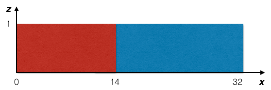
In order to achieve effective comparisons with [8], two-dimensional simulations with slip boundary conditions have been performed. The performance of our model has been evaluated by comparing density contours and, more quantitatively, different kinds of energy budgets. In particular, we have computed the time evolution of the normalized potential, kinetic and dissipated energies integrated over the whole domain. The potential energy is:

$$E_{p}(t)=\int_{\Omega}\frac{1}{Fr^{2}}\rho zdV.$$ (64)

The kinetic energy is:

$$E_{k}(t)=\int_{\Omega}\frac{1}{2}\rho u_{i}u_{i}dV,$$ (65)

while the time evolution of the dissipated energy is computed by solving the following equation:

$$\frac{dE_{d}}{dt}=\int_{\Omega}\biggl{\{}\mu\biggl{[}\frac{1}{2}(\partial_{j}u_{i}+\partial_{i}u_{j})^{2}-\frac{2}{3}(\nabla\cdot\textbf{u})^{2}\biggr{]}\biggr{\}}dV.$$ (66)

As proposed in [8] the quantity $E_{amb}$ is computed as:

$$E_{amb}=\frac{1}{1-\gamma_{r}}\int_{\Omega}\gamma_{r}zdV.$$ (67)

From the initial potential energy, by subtracting $E_{amb}$, we obtain $E_{p0}^{a}$ (defined in [8] as initial available potential energy):

$$E_{p0}^{a}=E_{p0}-E_{amb}$$ (68)

and the available potential energy at a generic time $t$:

$$E_{p}^{a}(t)=E_{p}(t)-E_{amb}.$$ (69)

We then normalize each contribution to the overall energy budget with $E_{p0}^{a}$ and we obtain the normalized potential energy $E_{p}^{n}(t)=E_{p}^{a}(t)/E_{p0}^{a}$, the normalized kinetic energy $E_{k}^{n}(t)=E_{k}(t)/E_{p0}^{a}$ and the normalized dissipated energy $E_{d}^{n}(t)=E_{d}(t)/E_{p0}^{a}$. The second energy budget taken into consideration provides the evaluation of the energies dissipated by the dense and the light front separately, as suggested in [8]. The energy dissipated by the light front is computed using the following equation:

$$\frac{dE_{d}^{light}(t)}{dt}=\int_{0}^{x_{0}}\int_{0}^{1}\mu\biggl{[}\frac{1}{2}(\partial_{j}u_{i}+\partial_{i}u_{j})^{2}-\frac{2}{3}(\nabla\cdot\textbf{u})^{2}\biggr{]}\biggr{\}}dzdx,$$ (70)

while the energy dissipated by the dense front is:

$$\frac{dE_{d}^{dense}(t)}{dt}=\int_{x_{0}}^{L}\int_{0}^{1}\mu\biggl{[}\frac{1}{2}(\partial_{j}u_{i}+\partial_{i}u_{j})^{2}-\frac{2}{3}(\nabla\cdot\textbf{u})^{2}\biggr{]}\biggr{\}}dzdx.$$ (71)

where $x_{0}$ is the abscissa of the initial discontinuity.

5.1 Direct Numerical Simulations

For the fully resolved simulations, a grid composed by approximately $37000$ elements has been employed. The polynomial degree has been set equal to $4,$ while the polynomial degree associated to the test filter operation was taken to be $2.$ Notice that, with these choices, the total number of degrees of freedom is of the same order of magnitude as that in [8].

In Figure 2 we compare the density contours obtained from our compressible NS simulations with the corresponding density contours obtained in [8], for density ratios $\gamma_{r}=0.2,0.7$, at $t=10$ and for $Re=4000$. For both density ratios the results are quite similar, both in terms of the position of the front and of the number and appearance of the Kelvin-Helmoltz billows. In particular, considering the lower density ratio $\gamma_{r}=0.2$ (Figures 2-2) we notice that, as in [8], the dense front presents a considerably lower height and that, by $t=10$, it has propagated further with respect to the light front. Moreover, by decreasing the density ratio, we observe that the vortical structures appear to be confined to the region near the dense front. According to the explanation in [8], this is because across the dense current the velocity difference and the shear are larger, which has destabilizing effect.

In the case of $\gamma_{r}=0.2$ we notice however some discrepancies between our results and those of [8]. The length of the area of the density current interested by the presence of Kelvin-Helmoltz billows is more extended in our case: the first vortex is located approximately at $x=13$ in our simulation (see Figure 2) while its position is $x=15$ in [8] (Figure 2).

Figure 2: Density contours at $t=10$ for $Re=4000$ (DNS) (a) DG simulation, $\gamma_{r}=0.7$ (b)[8], $\gamma_{r}=0.7$ (c) DG simulation, $\gamma_{r}=0.2$ (d) [8], $\gamma_{r}=0.2$

Another important feature which is correctly reproduced by the DG simulations is the behaviour of the density current in the presence of constant dynamic viscosity (see Figure 3). In this situation the formation of vortexes is limited to a smaller region close to the dense front (as highlighted in [8]).

Figure 3: Density contours at $t=10$ for $\gamma_{r}=0.2$ and $Re=4000$ (DNS) with constant dynamic viscosity $\mu=1/Re$.

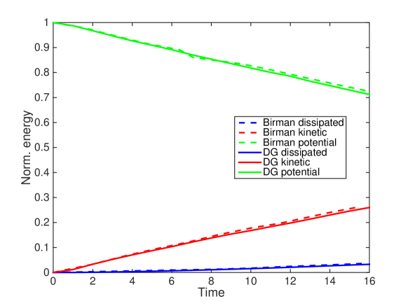
Considering energy budgets, in Figure 4 we present the time evolution of the normalized potential energy $E_{p}^{n}(t)$, the normalized kinetic energy $E_{k}^{n}(t)$ and the normalized dissipated energy $E_{d}^{n}(t)$ up to $t=10$, for $Re=4000$ and density ratio $\gamma_{r}=0.4$. We notice that the time evolution of the different energy budgets reported in [8] (dashed lines) is very well captured by the DG simulation (continuous lines).

Figure 4: Time evolution of the normalized potential energy $E_{p}^{n}$ (green), normalized kinetic energy $E_{k}^{n}$ (red) and normalized dissipated energy $E_{d}^{n}$ (blue) for $\gamma_{r}=0.4$ and $Re=4000$ (DNS). Continuous lines: DG simulation. Dashed lines: [8] simulation.

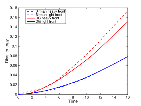
In Figure 5 we show the time evolution of the energies dissipated by the light and the dense front, respectively. Both in [8] (dashed lines) and in DG our simulation (continuous lines), the dense front (red lines) is more dissipative with respect to the light front (blue lines). However, a slight underestimation of the energy dissipated by the dense front is present in the DG simulation.

Figure 5: Time evolution of the energies dissipated by the dense (red) and light (blue) fronts for $\gamma_{r}=0.4$ and $Re=4000$ (DNS). Continuous lines: DG simulation. Dashed lines: [8] simulation.

5.2 Large Eddy Simulations

Besides simulations at DNS resolution, also some Large Eddy Simulation experiments have been carried out in the lock-exchange test-case, using a density ratio $\gamma_{r}=0.7$ and Reynolds number $Re=40000.$ These experiments have been performed employing the same computational grid and the same polynomial degree as in the DNS at $Re=4000$. Both the classic Smagorinsky model and the Germano dynamic model have been considered, together with an under-resolved DNS obtained without employing any model. For this case, the simulation could be completed without having to add any artificial diffusion.

In Figure 6 we show the dissipated energy as a function of time for the different models. We notice that the Smagorinsky model (red line) presents a much more dissipative behaviour with respect to the no-model (blue line) and the dynamic model (green line) simulations.

Figure 6: Time evolution of the normalized energies dissipated using no model (blue), the Smagorinsky model (red), the dynamic model (green) for $\gamma_{r}=0.7$ and $Re=40000$ (LES).

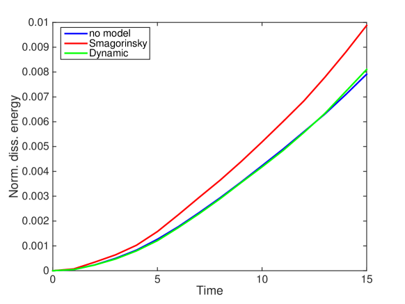
This behaviour of the Smagorinsky model is confirmed by the vorticity field at a fixed instant of time $t=15$ (see Figure 7). The vorticity field provided by the Smagorinsky model (Figure 7) is smoother and characterized by less vortical structures and lower vorticity peak values. As regard as the comparison between no-model and dynamic model we notice that, even if the dissipated energy does not evidence significant differences (as can be easily seen in Figure 6 observing the green and blue lines), a careful examination of Figure 7 allows to observe that the vorticity field obtained with the dynamic model (Figure 7) presents finer structures and higher vorticity peak values with respect to the no model case (Figure 7), suggesting that backscatter probably plays a quite important role when employing the dynamic model. This fact is confirmed also by considering the values of the dynamic constant $C_{s}$ at the same instant $t=15$ represented in Figure 8: there are indeed many elements where $C_{s}$ assumes negative values (indicated in blue) smaller than $-0.02$, with peak negative values of $-0.08$. These values are not negligible if compared to the value assumed by the Smagorinsky constant in the static Smagorinsky model which is $C_{s}=0.1$.

Figure 7: Vorticity field obtained for $\gamma_{r}=0.7$ and $Re=40000$ (LES) at $t=15$. Red: positive values. Blue: negative values. (a) No model, value range $[-63,77]$. (b) Smagorinsky model, value range $[-42,54]$. (c) Dynamic model, value range $[-74,85]$.

Figure 8: Dynamic constant $C_{s}$ for $\gamma_{r}=0.7$ and $Re=40000$ (LES) at $t=15$. Value range $[-0.08,0.1]$. Red: positive values. Blue: negative values.

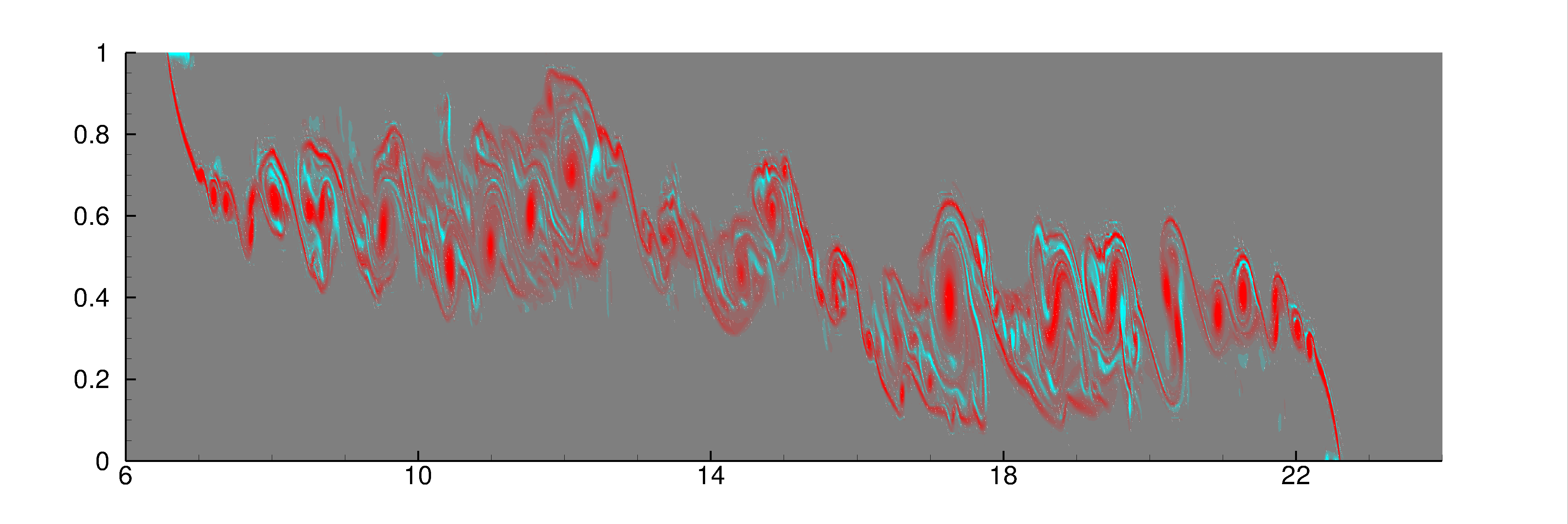
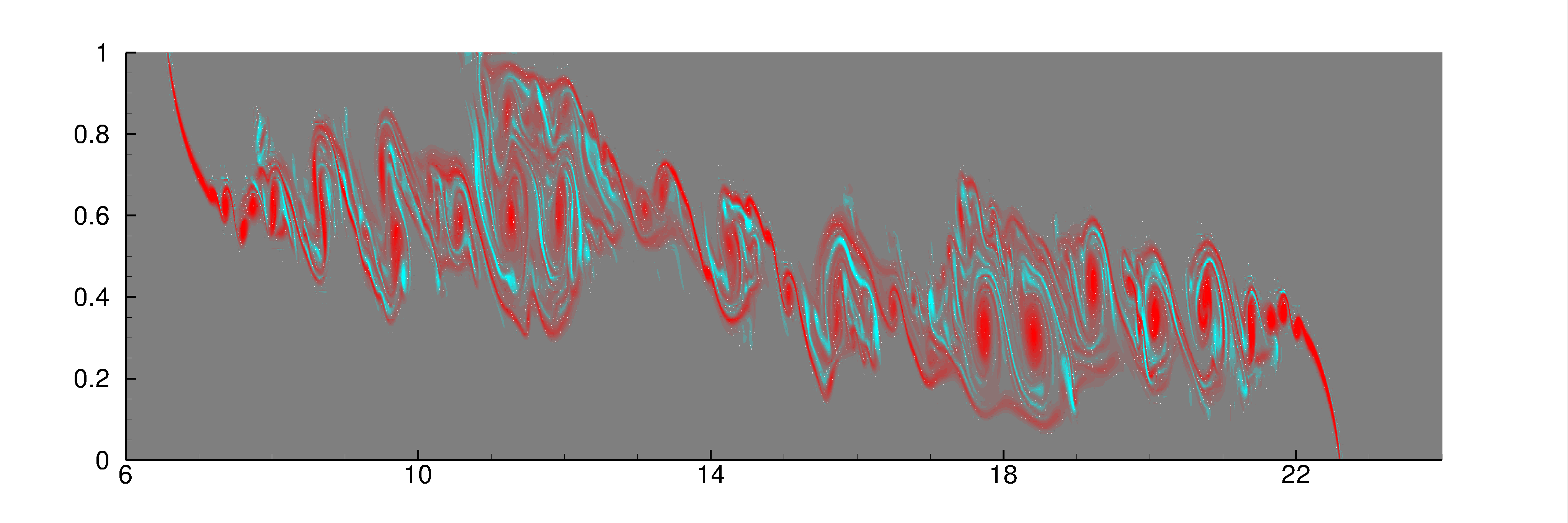
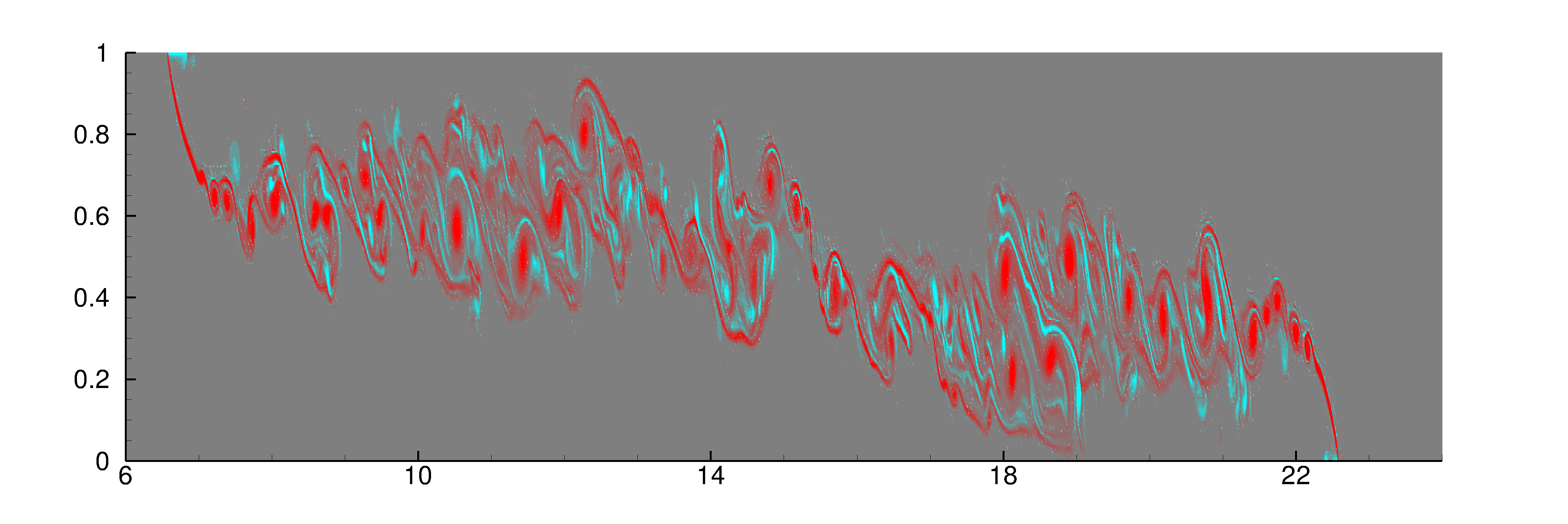
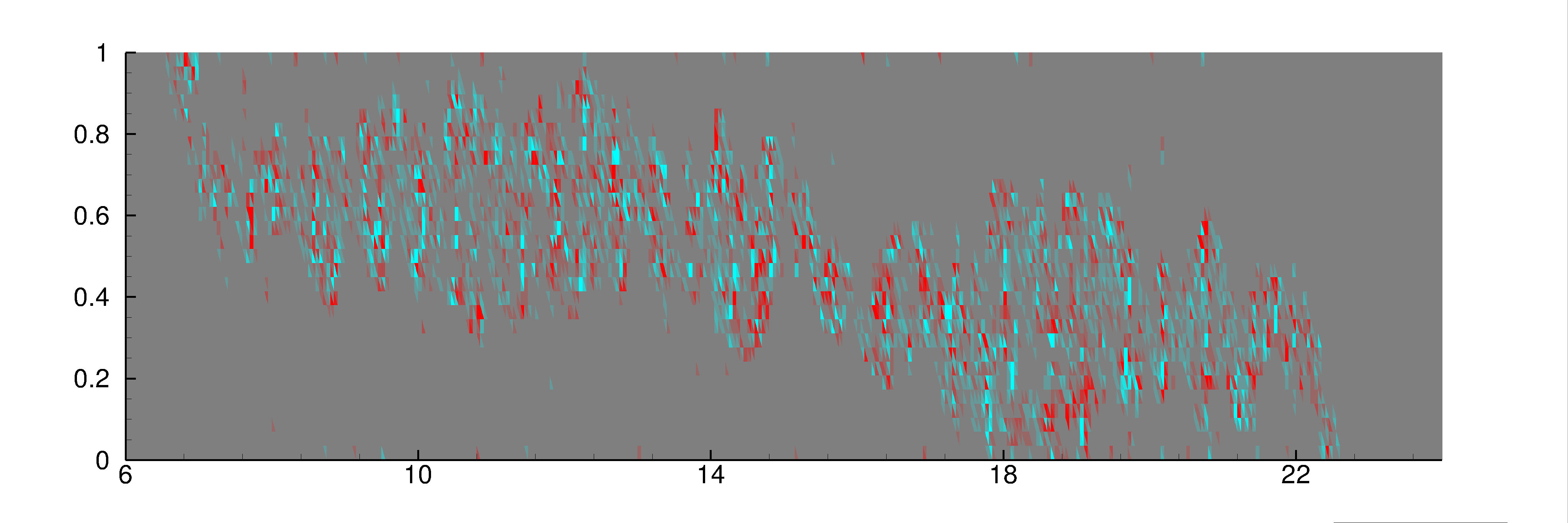
Notice that approximately $13500$ CPU hours have been necessary to carry out the DNS at $Re=4000$ till $t=15$ and that the same number of CPU hours has been employed for the under-resolved DNS at $Re=40000$. On the other hand, the Large Eddy Simulations at $Re=40000$ with the Smagorinsky model and with the dynamic procedure have required $20000$ and $22000$ CPU hours, respectively.

5.3 Impact of the numerical flux choice

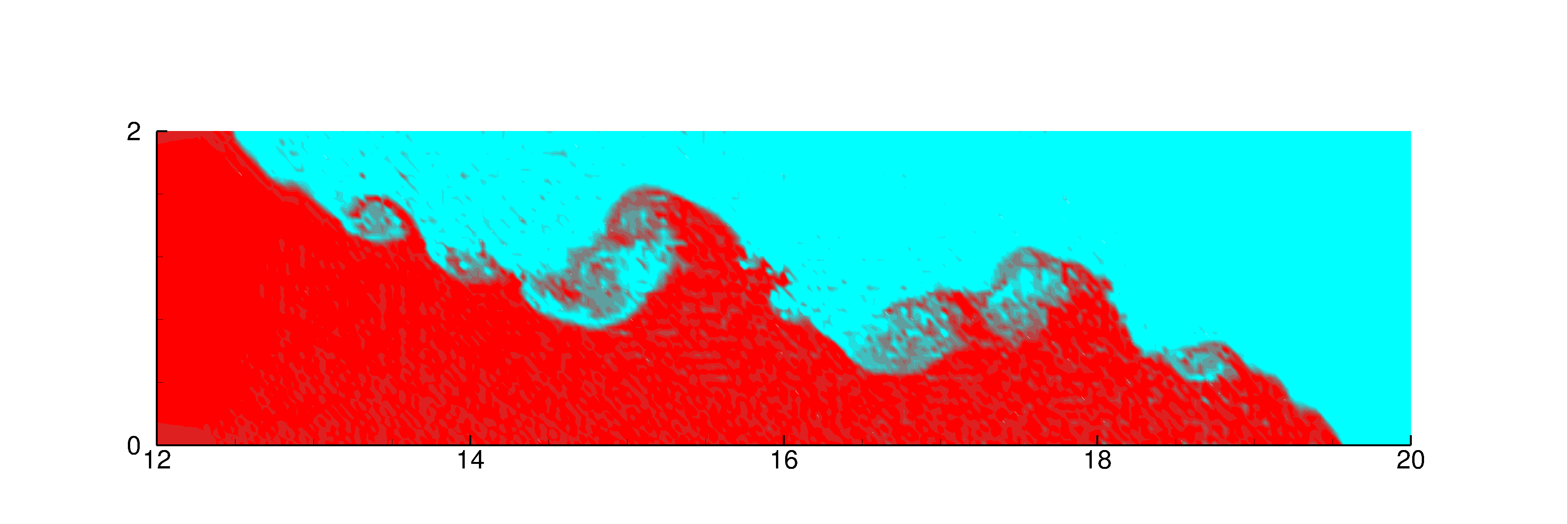
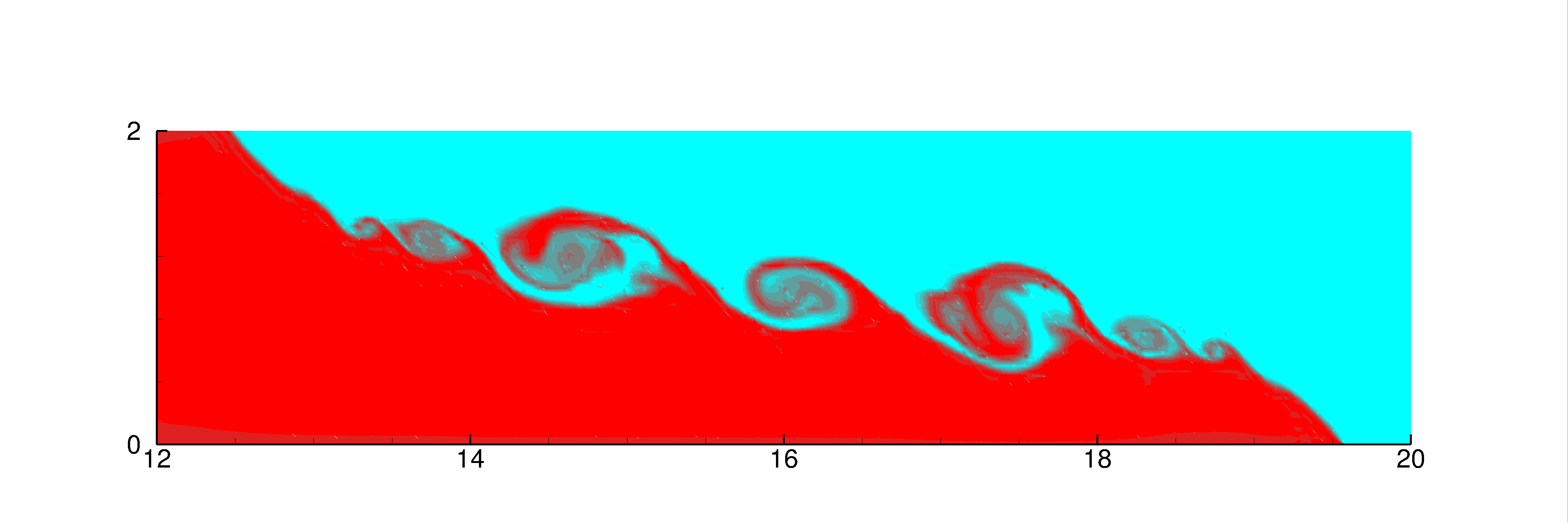
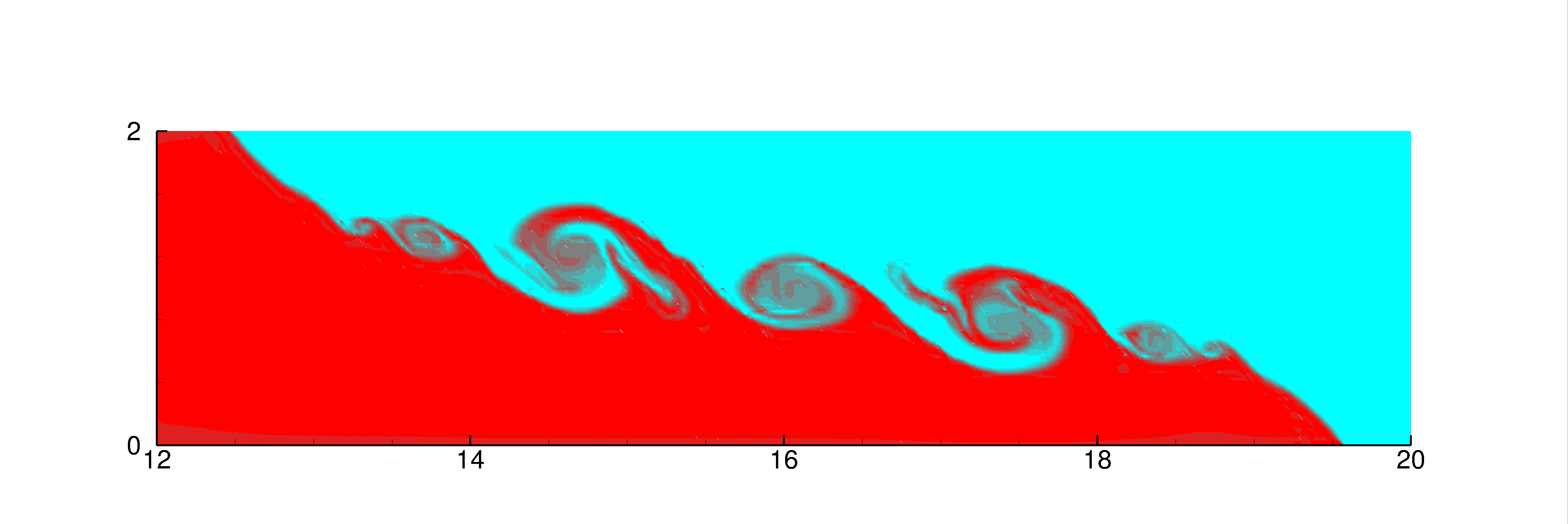
In this section some results obtained with the Rusanov numerical flux, a modified version of the Rusanov flux (where the upwinding velocity is set equal to the velocity of the fluid) and the exact Godunov Riemann solver (implemented as in [23]) will be presented. In particular, in Figure 9 we have the density profiles of a Boussinesq simulation for $Re=44721$ and $\gamma_{r}=0.96$, at $t=5$. We notice that the profile obtained with the Rusanov flux (Figure 9) is highly inaccurate both for the incorrect reproduction of the shape and number of turbulent structures and for the presence of spurious oscillations. These spurious features are instead absent in the profiles obtained with the exact Godunov Riemann solver and with the modified version of the Rusanov flux (Figures 9 and 9). This behaviour is probably due to the fact that, when dealing with low Mach number flows, the upwinding velocity in the Rusanov flux is equal to the sound velocity, which is very different from the velocity of the fluid in this regime. As a consequence, upwinding is performed with a wrong velocity. This difficulty is indeed overcame by employing the exact solver or simply by substituting the upwinding velocity with the velocity of the fluid. This explanation appears to be consistent with the accurate results obtained by upwind-based, semi-Lagrangian schemes in the simulation of variable density flows with small density differences, see e.g. [9], [30].

Figure 9: Density for $Re=44721$ and $\gamma_{r}=0.96$ at time $t=5$. (a) Rusanov flux. (b) Godunov exact Riemann solver. (c) Modified Rusanov flux (upwinding velocity equal to the velocity of the fluid)

6 Conclusions and future perspectives

In this paper, we have assessed the capability of a DG-LES model for the numerical simulation of turbulent gravity currents in the non-Boussinesq regime. The results obtained by application of the DG-LES method proposed in [1] have been compared with those presented in [8] in the incompressible case. The quality of our results with respect to [8] has been first assessed using density contours at a fixed instant of time and for different density ratios $\gamma_{r}$. The density contours obtained with our DG simulations appears to be qualitatively similar to the ones in [8] even though some discrepancies are present, especially for the lower density ratio $\gamma_{r}=0.2$.

From a more quantitative viewpoint, two different energy budgets have been considered. First of all, normalized values of potential, kinetic and dissipated energies as a function of time have been compared with the trends reported in [8], finding very good agreement. The temporal evolution of the energy dissipated separately by the light and dense fronts has also been computed. Also in this case, we have quite good agreement with the results in [8], with a good prediction of the more dissipative nature of the dense front with respect to the light one. There is however a slight underestimation of the energy dissipated by the dense front. We can conclude that our approach is able to reproduce quite well the incompressible results of [8] in the low Mach number regime. Some preliminary LES results have also been presented. Even if these results have not been compared to corresponding DNS results, we can infer that the classic Smagorinsky model is probably too dissipative for the accurate simulation of turbulent gravity currents. On the other hand the results obtained with the dynamic model seem to indicate that backscatter plays a quite important role. Concerning the impact of the numerical flux choice, we can conclude that the generally used Rusanov flux may not be the best option for variable density low Mach number regime.

From the physical point of view, the next planned step is to carry out Large Eddy Simulations employing also more advanced models, like the anisotropic dynamic model proposed in [2] and the novel proposals in [19] for compressible, variable density flows. Moreover, we have planned also to compute additional diagnostics, like the available potential energy ([31], [29]), in order to better discriminate the performances of the different models, as already done in [25], [7] and [6]. From the computational point of view, we are aware that employing an explicit time integration method in presence of low Mach numbers leads to computational inefficiency; the implementation of an implicit time integration method will be probably necessary in order to perform also 3D simulations. Furthermore, a deeper investigation of the influence of the numerical flux on the solutions in variable density low-Mach number would be required to better understand some of the results presented in this paper.

References

- [1] A. Abbà, L. Bonaventura, M. Nini, and M. Restelli. Dynamic models for Large Eddy Simulation of compressible flows with a high order DG method. Computers & Fluids, 122:209–222, 2015.
- [2] A. Abbà, C. Cercignani, and L. Valdettaro. Analysis of Subgrid Scale Models. Computer and Mathematics with Applications, 46:521–535, 2003.
- [3] D. N. Arnold, F. Brezzi, B. Cockburn, and L.D. Marini. Unified analysis of Discontinuous Galerkin methods for elliptic problems. SIAM Journal of Numerical Analysis, 39:1749–1779, 2002.
- [4] F. Bassi and S. Rebay. High Order Accurate Discontinuous Finite Element Method for the Numerical Solution of the Compressible Navier-Stokes Equations. Journal of Computational Physics, 131:267–279, 1997.
- [5] L. C. Berselli, P.F. Fischer, T. Iliescu, and T.M. Özgökmen. Horizontal Large Eddy Simulation of stratified mixing in a Lock-exchange system. Journal of Scientific Computing, 49:3–20, 2011.
- [6] L.C. Berselli, M. Cerminara, and T. Iliescu. Disperse Two-Phase Flows, with Applications to Geophysical Problems. Pure and Applied Geophysics, 172:181–196, 2014.
- [7] L.C. Berselli, P.F. Fischer, T. Iliescu, and T.M. Özgökmen. Horizontal Large Eddy Simulation of Stratified Mixing in a Lock-Exchange System. Journal of Scientific Computing, 49:3–20, 2011.
- [8] V. K. Birman, J.E. Martin, and E. Meiburg. The non-Boussinesq Lock-exchange problem. Part 2. High-resolution simulations. Journal of Fluid Mechanics, 537:125–144, 2005.
- [9] L. Bonaventura. A semi-implicit, semi-Lagrangian scheme using the height coordinate for a nonhydrostatic and fully elastic model of atmospheric flows. Journal of Computational Physics, 158:186–213, 2000.
- [10] P. Castillo, B. Cockburn, I. Perugia, and D. Schötzau. An a priori analysis of the Local Discontinuous Galerkin method for elliptic problems. SIAM Journal of Numerical Analysis, 38:1676–1706, 2000.
- [11] B. Cockburn and C.W. Shu. The Local Discontinuous Galerkin Method for Time-Dependent Convection Diffusion Systems. SIAM Journal of Numerical Analysis, 35:2440–2463, 1998.
- [12] S. S. Collis. Discontinuous Galerkin methods for turbulence simulation. In Proceedings of the 2002 Center for Turbulence Research Summer Program, pages 155–167, 2002.
- [13] S. S. Collis and Y. Chang. The DG/VMS method for unified turbulence simulation. AIAA paper, 3124:24–27, 2002.
- [14] R. Cools. An Encyclopaedia of Cubature Formulas. Journal of Complexity, 19:445–453, 2003.
- [15] F.van der Bos, J.J.W. van der Vegt, and B.J. Geurts. A multi-scale formulation for compressible turbulent flows suitable for general variational discretization techniques. Computational Methods in Applied Mechanical Engineering, 196:2863–2875, 2007.
- [16] FEMilaro, a finite element toolbox. https://bitbucket.org/mrestelli/femilaro/wiki/Home. Available under GNU GPL v3.
- [17] E. Garnier, N. Adams, and P. Sagaut. Large Eddy Simulation for Compressible Flows. Springer Verlag, 2009.
- [18] M. Germano. Turbulence: the filtering approach. Journal of Fluid Mechanics, 238:325–336, 1992.
- [19] M. Germano, A. Abbà, R. Arina, and L. Bonaventura. On the extension of the eddy viscosity model to compressible flows. Physics of Fluids, 2014.
- [20] M. Germano, U. Piomelli, P. Moin, and W.H. Cabot. A Dynamic Subgrid-Scale Eddy Viscosity Model. Physics of Fluids, 3(7):1760–1765, 1991.
- [21] A.E. Gill. Atmosphere-Ocean Dynamics. Academic Press, 1982.
- [22] F.X. Giraldo and M. Restelli. A study of spectral element and discontinuous galerkin methods for the navier-stokes equations in nonhydrostatic mesoscale atmospheric modelling: equation sets and test cases. Journal of Computational Physics, 227:3849–3877, 2008.
- [23] J.J. Gottlieb and C.P.T. Groth. Assessment of Riemann Solvers for Unsteady One-Dimensional Inviscid FLows of Perfect Gases. Journal of Computational Physics, 78:437–458, 1988.
- [24] W. Houf and R. Schefer. Analytical and experimental investigation of small scale unintended releases of hydrogen. International Journal of Hydrogen Energy, 33:1435–1444, 2008.
- [25] T.M. Özgökmen, T. Iliescu, and P.F. Fischer. Large Eddy Simulation of stratified mixing in a three-dimensional Lock-exchange system. Ocean Modelling, 26:134–155, 2009.
- [26] T.M. Özgökmen, T. Iliescu, P.F. Fischer, A. Srinivasan, and J. Duan. Large Eddy Simulation of stratified mixing in two-dimensional dam-break problem in a rectangular enclosed domain. Ocean Modelling, 16:106–140, 2006.
- [27] P. Sagaut. Large Eddy Simulation for Incompressible Flows: An Introduction. Springer Verlag, 2006.
- [28] H. Schlichting. Boundary-layer theory.7th edition. McGraw-Hill, 1979.
- [29] Y. Tseng and J.H. Ferziger. Mixing and available potential energy in stratified flows. Physics of Fluids, 13:1281–1293, 2001.
- [30] G. Tumolo and L. Bonaventura. A semi-implicit, semi-Lagrangian, DG framework for adaptive numerical weather prediction. Quarterly Journal of the Royal Meteorological Society, 141:2582–2601, 2015.
- [31] K.B. Winters, P.N. Lombard, J.J. Riley, and E.A. D’Asaro. Available potential energy and mixing in density-stratified fluids. Journal of Fluid Mechanics, 289:115–128, 1995.