Parallel numerical modeling of hybrid-dimensional compositional non-isothermal Darcy flows in fractured porous media

Abstract

This paper introduces a new discrete fracture model accounting for non-isothermal compositional multiphase Darcy flows and complex networks of fractures with intersecting, immersed and non immersed fractures. The so called hybrid-dimensional model using a 2D model in the fractures coupled with a 3D model in the matrix is first derived rigorously starting from the equi-dimensional matrix fracture model. Then, it is discretized using a fully implicit time integration combined with the Vertex Approximate Gradient (VAG) finite volume scheme which is adapted to polyhedral meshes and anisotropic heterogeneous media. The fully coupled systems are assembled and solved in parallel using the Single Program Multiple Data (SPMD) paradigm with one layer of ghost cells. This strategy allows for a local assembly of the discrete systems. An efficient preconditioner is implemented to solve the linear systems at each time step and each Newton type iteration of the simulation. The numerical efficiency of our approach is assessed on different meshes, fracture networks, and physical settings in terms of parallel scalability, nonlinear convergence and linear convergence.

1 Introduction

Flow and transport in fractured porous media are of paramount importance for many applications such as petroleum exploration and production, geological storage of carbon dioxide, hydrogeology, or geothermal energy. Two classes of models, dual continuum and discrete fracture models, are typically employed and possibly coupled to simulate flow and transport in fractured porous media. Dual continuum models assume that the fracture network is well connected and can be homogeneized as a continuum coupled to the matrix continuum using transfer functions. On the other hand, discrete fracture models (DFM), on which this paper focuses, represent explicitly the fractures as codimension one surfaces immersed in the surrounding matrix domain. The use of lower dimensional rather than equi-dimensional entities to represent the fractures has been introduced in [1], [2], [3], [4], [5] to facilitate the grid generation and to reduce the number of degrees of freedom of the discretized model. The reduction of dimension in the fracture network is obtained from the equi-dimensional model by integration and averaging along the width of each fracture. The resulting so called hybrid-dimensional models couple the 3D model in the matrix with a 2D model in the fracture network taking into account the jump of the normal fluxes as well as additional transmission conditions at the matrix fracture interfaces. These transmission conditions depend on the mathematical nature of the equi-dimensional model and on additional physical assumptions. They are typically derived for a single phase Darcy flow for which they specify either the continuity of the pressure in the case of fractures acting as drains (see [1], [6]) or Robin type conditions in order to take into account the discontinuity of the pressure for fractures acting as barriers (see [2], [5], [7], [8]). Different transmission conditions are derived in [9] in the case of a linear hyperbolic equation, and in [10], [11], [12], [13], [14] in the case of two-phase immiscible Darcy flows.

The discretization of hybrid-dimensional Darcy flow models has been the object of many works. In [4] a cell-centred Finite Volume scheme using a Two Point Flux Approximation (TPFA) is proposed assuming the orthogonality of the mesh and isotropic permeability fields. Cell-centred Finite Volume schemes can be extended to general meshes and anisotropic permeability fields using MultiPoint Flux Approximations (MPFA) (see [15], [16], [17], [18], [19]). MPFA schemes can lack robustness on distorted meshes and large anisotropies due to the non symmetry of the discretization. They are also very expensive compared with nodal discretizations on tetrahedral meshes. In [1], a Mixed Finite Element (MFE) method is proposed for single phase Darcy flows. It is extended to two-phase flows in [11] in an IMPES framework using a Mixed Hybrid Finite Element (MHFE) discretization for the pressure equation and a Discontinuous Galerkin discretization of the saturation equation. The Hybrid Finite Volume and Mimetic finite difference schemes, belonging to the family of Hybrid Mimetic Mixed Methods (HMM) [20], have been extended to hybrid-dimensional models in [21], [22] as well as in [6], [8] in the more general Gradient Discretization framework [23]. These approaches are adapted to general meshes and anisotropy but require as many degrees of freedom as faces. Control Volume Finite Element Methods (CVFE) [3], [10], [24], [15] have the advantage to use only nodal unknowns leading to much fewer degrees of freedom than MPFA and HMM schemes on tetrahedral meshes. On the other hand, at the matrix fracture interfaces, the control volumes have the drawback to be shared between the matrix and the fractures. It results that a strong refinement of the mesh is needed at these interfaces in the case of large contrasts between the matrix and fracture permeabilities. This article focus on the Vertex Approximate Gradient (VAG) scheme which has been introduced for the discretization of multiphase Darcy flows in [25] and extended to hybrid-dimensional models in [13], [6], [8], [9], [14]. The VAG scheme uses nodal and fracture face unknowns in addition to the cell unknowns which can be eliminated without any fill-in. Thanks to its essentially nodal feature, it leads to a sparse discretization on tetrahedral or mainly tetrahedral meshes. It has the advantage, compared with the CVFE methods of [3], [10], [24] or [26], to avoid the mixing of the control volumes at the matrix fracture interfaces, which is a key feature for its coupling with a transport model. As shown in [13] for two-phase flow problems, this allows for a coarser mesh size at the matrix fracture interface for a given accuracy. Let us also mention that non-matching discretizations of the fracture and matrix meshes are studied for single phase Darcy flows in [27], [28], [29] and [30].

The first objective of this paper is to extend the derivation of the hybrid-dimensional model to the case of non-isothermal compositional multiphase Darcy flows. To focus on compositional non-isothermal features, capillary pressures are not considered in this paper. They could be included following the usual phase based upwinding approach as in [25] or recent ideas developed in [31] for two-phase flows. Let us refer to [32] for a comparison of both approaches in the case of an immiscible two-phase flow using a reference solution provided by the equi-dimensional model in the fractures. All the underlying assumptions of our reduced model will be carefully stated. In particular, the fractures are considered as pervious and are assumed not to act as barriers. It results, as in [1], that the pressure can be considered as continuous at the matrix fracture interfaces. The hybrid-dimensional model accounts for complex network of fractures including intersecting, immersed and non immersed fractures. The formulation of the compositional model is based on a Coats’ type formulation [33], [34] extending the approach presented in [25] to non-isothermal flows. It accounts for an arbitrary nonzero number of components in each phase allowing to model immiscible, partially miscible or fully miscible flows.

The second objective of this paper is to extend the VAG discretization to our model and to develop an efficient parallel algorithm implementing the discrete model. Following [25], [13], the discretization is based on a finite volume formulation of the component molar and energy conservation equations. The definition of the control volumes is adapted to the heterogeneities of the porous medium and avoids in particular the mixing of matrix and fracture rocktypes for the degrees of freedom located at the matrix fracture interfaces. The fluxes combine the VAG Darcy and Fourier fluxes with a phase based upwind approximation of the mobilities. A fully implicit Euler time integration coupling the conservation equations with the local closure laws including thermodynamical equilibrium is used in order to avoid severe limitations on the time step due to the high velocities and small control volumes in the fractures.

The discrete model is implemented in parallel based on the SPMD (Single Program, Multiple Data) paradigm. It relies on a distribution of the mesh on the processes with one layer of ghost cells in order to allow for a local assembly of the discrete systems. The key ingredient for the efficiency of the parallel algorithm is the solution, at each time step and at each Newton type iteration, of the large sparse linear system coupling the physical unknowns on the spatial degrees of freedom of the VAG scheme. Our strategy is first based on the elimination, without any fill-in, of both the local closure laws and the cell unknowns. Then, the reduced linear system is solved using a parallel iterative solver preconditioned by a CPR-AMG preconditioner introduced in [35] and [36]. This state of the art preconditioner combines multiplicatively an Algebraic MultiGrid (AMG) preconditioner for a proper pressure block of the linear system with a local incomplete factorization preconditioner for the full system. The numerical efficiency of the algorithm, in terms of parallel scalability, nonlinear convergence and linear convergence, is investigated on several test cases. We consider different families of meshes and different complexity of fracture networks ranging from a few fractures to say about 1000 fractures with highly contrasted matrix fracture permeabilities. The test cases incorporate different physical models including one isothermal immiscible two-phase flow, one isothermal Black Oil two-phase flow model, as well as three non-isothermal water component liquid gas flow models.

This paper is organized as follows. In section 2, the hybrid-dimensional non-isothermal compositional multiphase Darcy flow model is derived from the equi-dimensional model. In Section 3, the VAG discretization is briefly recalled and then extended to our model. The parallel algorithm is detailed in section 4. Section 5 is devoted to the test cases including the numerical investigation of the parallel scalability of the algorithm.

2 Hybrid-dimensional compositional non-isothermal Darcy flow model

This section deals with the modeling and the formulation of non-isothermal compositional multiphase Darcy flows in fractured porous media. The fractures are represented as surfaces of co-dimension one immersed in the surrounding three dimensional matrix domain. The 2D Darcy flow in the fracture network is coupled with the 3D Darcy flow in the matrix domain, hence the terminology of hybrid-dimensional model. The reduction of dimension in the fracture is obtained by extension to non-isothermal compositional flows of the methodology introduced in [1], [2], [5] for single phase Darcy flows. Complex networks of fractures are considered including immersed, non immersed and intersecting planar fractures. The formulation of the compositional model is based on a Coats’ type formulation [33] extending to non-isothermal flows the approach presented in [25]. It accounts for an arbitrary nonzero number of components in each phase allowing to model immiscible, partially miscible or fully miscible flows. To focus on the compositional and non-isothermal aspects, we consider a Darcy flow model without capillary pressures. The capillary pressures including different rocktypes at the matrix fracture interface can be taken into account in the framework of the VAG scheme following the usual phase based upwinding of the mobilities as in [25]. An alternative approach is proposed in [31] for two-phase flows in order to capture the jump of the saturations at the matrix fracture interface $\Gamma$ due to discontinuous capillary pressure curves. These two choices are compared in [32] to a reference solution provided by an equi-dimensional model in the fractures. It is shown that the second choice provides a better solution as long as the matrix acts as a barrier since it captures the saturation jump. On the other hand, the first choice provides a more accurate solution when the non wetting phase goes out of the fractures since the mean capillary pressure in the fractures is better approximated.

2.1 Extended Coats’ formulation of non-isothermal compositional models

Let us denote by ${\cal P}$ the set of phases and by ${\cal C}$ the set of components. Each phase $\alpha\in{\cal P}$ is described by its non empty subset of components ${\cal C}^{\alpha}\subset{\cal C}$ in the sense that it contains the components $i\in{\cal C}^{\alpha}$. It is assumed that, for any $i\in{\cal C}$, the set of phases containing the component $i$

$${\cal P}_{i}=\{\alpha\in{\cal P}\,|\,i\in{\cal C}^{\alpha}\}.$$

is non empty. The thermodynamical properties of each phase $\alpha\in{\cal P}$ depend on the pressure $P$, the temperature $T$, and the molar fractions

$$C^{\alpha}=\left(C_{i}^{\alpha}\right)_{i\in{\cal C}^{\alpha}}.$$

For each phase $\alpha\in{\cal P}$, we denote by $\zeta^{\alpha}(P,T,C^{\alpha})$ the molar density, by $\rho^{\alpha}(P,T,C^{\alpha})$ the mass density, by $\mu^{\alpha}(P,T,C^{\alpha})$ the dynamic viscosity, by $f_{i}^{\alpha}(P,T,C^{\alpha})$, $i\in{\cal C}^{\alpha}$ the fugacity coefficients, by $e^{\alpha}(P,T,C^{\alpha})$ the molar internal energy, and by $h^{\alpha}(P,T,C^{\alpha})$ the molar enthalpy. The relative permeabilities are denoted for each phase $\alpha\in{\cal P}$ by $k_{r}^{\alpha}(S)$ where $S=(S^{\alpha})_{\alpha\in{\cal P}}$ is the vector of the phase volume fractions (saturations). The model takes into account phase change reactions which are assumed to be at equilibrium. It results that phases can appear or disappear. Therefore, we denote by $Q\subset{\cal P}$, $Q\neq\emptyset$ the unknown representing the set of present phases. For a given set of present phases $Q$, it may occur that a component $i\in{\cal C}$ does not belong to the subset $\bigcup_{\alpha\in Q}{\cal C}^{\alpha}$ of ${\cal C}$. Hence, we define the subset of absent components as a function of $Q$ by

$$\overline{\cal C}_{Q}=\{i\in{\cal C}\,|\,Q\cap{\cal P}_{i}=\emptyset\}.$$

Following [33], [34], [25], the extended non-isothermal Coats’ formulation relies on the the so-called natural variables and uses the set of unknowns

$$X=\Bigl{(}P,T,S^{\alpha},C^{\alpha},\alpha\in Q,n_{i},i\in\overline{\cal C}_{Q},Q\Bigr{)}.$$

The saturations are implicitely set to $S^{\alpha}=0$ for all absent phases $\alpha\in{\cal P}\setminus Q$. Let us denote by $n_{i}(X)$ the number of moles of the component $i\in{\cal C}$ per unit pore volume defined as the independent unknown $n_{i}$ for $i\in\overline{\cal C}_{Q}$ and as

$$n_{i}(X)=\sum_{\alpha\in Q\cap{\cal P}_{i}}\zeta^{{}^{\alpha}}(P,T,C^{\alpha})~{}S^{\alpha}~{}C_{i}^{\alpha}$$

for $i\in{\cal C}\setminus\overline{\cal C}_{Q}$. The fluid energy per unit pore volume is denoted by

$$E(X)=\sum_{\alpha\in Q}\zeta^{\alpha}(P,T,C^{\alpha})S^{\alpha}e^{\alpha}(P,T,C^{\alpha}),$$

and the rock energy per unit rock volume is denoted by $E_{r}(P,T)$. For each phase $\alpha\in Q$, we denote by $m_{i}^{\alpha}(X)$ the mobility of the component $i\in{\cal C}^{\alpha}$ in phase $\alpha\in Q$ with

$$m_{i}^{\alpha}(X)=C^{\alpha}_{i}\zeta^{\alpha}(P,T,C^{\alpha})\frac{k_{r}^{\alpha}(S)}{\mu^{\alpha}(P,T,C^{\alpha})},$$

and by

$$m^{\alpha}_{e}(X)=h^{\alpha}(P,T,C^{\alpha})\zeta^{\alpha}(P,T,C^{\alpha})\frac{k_{r}^{\alpha}(S)}{\mu^{\alpha}(P,T,C^{\alpha})}$$

the flowing enthalpy in phase $\alpha\in Q$. The generalized Darcy velocity of the phase $\alpha\in Q$ is

$$\frac{k_{r}^{\alpha}(S)}{\mu^{\alpha}(P,T,C^{\alpha})}{\bf V}^{\alpha}\ \mathrm{with}\ {\bf V}^{\alpha}=-{\bf K}\Bigl{(}\nabla P-\rho^{\alpha}(P,T,C^{\alpha}){\bf g}\Bigr{)},$$

where ${\bf g}$ is the gravitational acceleration. The total molar flux of the component $i\in{\cal C}\setminus\overline{\cal C}_{Q}$ is denoted by

$${\bf q}_{i}=\sum_{\alpha\in Q\cap{\cal P}_{i}}m^{\alpha}_{i}(X){\bf V}^{\alpha},$$

and the energy flux is defined as

$${\bf q}_{e}=\sum_{\alpha\in Q}m_{e}^{\alpha}(X){\bf V}^{\alpha}-\lambda\nabla T,$$

where $\lambda$ is the thermal conductivity of the fluid and rock mixture.

The system of equations accounts for the molar conservation for each component $i\in{\cal C}$ and the energy conservation

$$\begin{split}\phi\partial_{t}n_{i}&+\mathrm{div}({\bf q}_{i})=0,\,i\in{\cal C},\\ \phi\partial_{t}E+(1-\phi)\partial_{t}E_{r}&+{\mbox{\rm div}}({\bf q}_{e})=0,\end{split}$$ (1)

coupled to the following local closure laws including the thermodynamical equilibrium for each component $i$ present in at least two phases among the set of present phases $Q$

$$\begin{split}\displaystyle{\sum_{\alpha\in Q}S^{\alpha}}=&1,\\ \displaystyle{\sum_{i\in{\cal C}^{\alpha}}C_{i}^{\alpha}}=&1,\,\,\alpha\in Q,\\ f_{i}^{\alpha}(P,T,C^{\alpha})C_{i}^{\alpha}=&f_{i}^{\beta}(P,T,C^{\beta})C_{i}^{\beta},\,\,\alpha\neq\beta,(\alpha,\beta)\in(Q\cap{\cal P}_{i})^{2}.\,\,i\in{\cal C}.\end{split}$$ (2)

The system is closed with an additional equation for the discrete unknown $Q$ which is typically obtained by a flash calculation or by simpler criteria depending on the specific thermodynamical system. It provides the fixed point equation denoted by

$$Q=Q_{flash}(X).$$

2.2 Discrete fracture network

Let $\Omega$ denote a bounded domain of $\mathbb{R}^{3}$ assumed to be polyhedral. Following [1], [2], [5], [6], [8] the fractures are represented as interfaces of codimension 1. Let $J$ be a finite set and let $\overline{\Gamma}=\bigcup_{j\in J}\overline{\Gamma}_{j}$ and its interior $\Gamma=\overline{\Gamma}\setminus\partial\overline{\Gamma}$ denote the network of fractures $\Gamma_{j}\subset\Omega$, $j\in J$, such that each $\Gamma_{j}$ is a planar polygonal simply connected open domain included in an oriented plane of $\mathbb{R}^{3}$.

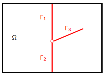
Figure 1: Example of a 2D domain with 3 intersecting fractures $\Gamma_{1},\Gamma_{2},\Gamma_{3}$.

The fracture width is denoted by $d_{f}$ and is such that $0<\underline{d}_{f}\leq d_{f}({\bf x})\leq\overline{d}_{f}$ for all ${\bf x}\in\Gamma$. We can define, for each fracture $j\in J$, its two sides $+$ and $-$. For scalar functions on $\Omega$, possibly discontinuous at the interface $\Gamma$ (typically in $H^{1}(\Omega\setminus\overline{\Gamma})$, we denote by $\gamma^{\pm}$ the trace operators on the side $\pm$ of $\Gamma$. Continuous scalar functions $u$ at the interface $\Gamma$ (typically in $H^{1}(\Omega)$) are such that $\gamma^{+}u=\gamma^{-}u$ and we denote by $\gamma$ the trace operator on $\Gamma$ for such functions. At almost every point of the fracture network, we denote by ${\bf n}^{\pm}$ the unit normal vector oriented outward to the side $\pm$ of $\Gamma$ such that ${\bf n}^{+}+{\bf n}^{-}=0$. For vector fields on $\Omega$, possibly discontinuous at the interface $\Gamma$ (typically in $H_{\mbox{\rm div}}(\Omega\setminus\overline{\Gamma})$, we denote by $\gamma_{n}^{\pm}$ the normal trace operator on the side $\pm$ of $\Gamma$ oriented outward to the side $\pm$ of $\Gamma$.

The gradient operator in the matrix domain $\Omega\setminus\overline{\Gamma}$ is denoted by $\nabla$ and the tangential gradient operator on the fracture network is denoted by $\nabla_{\tau}$ such that

$$\nabla_{\tau}u=\nabla u-(\nabla u\cdot{\bf n}^{+}){\bf n}^{+}.$$

We also denote by ${\mbox{\rm div}}_{\tau}$ the tangential divergence operator on the fracture network, and by $d\tau({\bf x})$ the Lebesgue measure on $\Gamma$.

We denote by $\Sigma$ the dimension $1$ open set defined by the intersection of the fractures excluding the boundary of the domain $\Omega$, i.e. the interior of $\bigcup_{\{(j,j^{\prime})\in J\times J\,|\,j\neq j^{\prime}\}}\partial\Gamma_{j}\cap\partial\Gamma_{j^{\prime}}\setminus\partial\Omega$.

For the matrix domain, Dirichlet (subscript $D$) and Neumann (subscript $N$) boundary conditions are imposed on the two dimensional open sets $\partial\Omega_{D}$ and $\partial\Omega_{N}$ respectively where $\partial\Omega_{D}\cap\partial\Omega_{N}=\emptyset$, $\partial\Omega=\overline{\partial\Omega_{D}}\cup\overline{\partial\Omega_{N}}$. Similarly for the fracture network, the Dirichlet and Neumann boundary conditions are imposed on the one dimensional open sets $\partial\Gamma_{D}$ and $\partial\Gamma_{N}$ respectively where $\partial\Gamma_{D}\cap\partial\Gamma_{N}=\emptyset$, $\overline{\partial\Gamma\cap\partial\Omega}=\overline{\partial\Gamma_{D}}\cup\overline{\partial\Gamma_{N}}$.

2.3 Hybrid-dimensional model for a two-phase flow example

For the sake of clarity, in this subsection, we first extend the hybrid-dimensional model proposed in [1], [2], [5] in the case of a single phase Darcy flow to the case of a two-phase Darcy flow.

Let us denote by $\langle\rangle_{\Gamma}$ the averaging operator in the width of the fracture in the normal direction, and let us set $S^{\alpha}_{f}=\langle S^{\alpha}\rangle_{\Gamma}$ and $P_{f}=\langle P\rangle_{\Gamma}$. In order to explain our construction of the hybrid-dimensional model from the equi-dimensional model, let us consider the following immiscible, incompressible isothermal two-phase flow model on the full domain $\Omega$ with 3D fractures

$$\phi\partial_{t}S^{\alpha}+{\mbox{\rm div}}({\bf q}^{\alpha})=0,\,\alpha=1,2,$$

with constant dynamic viscosities $\mu^{\alpha}$, $\alpha=1,2$ and the following Darcy two-phase velocities

$${\bf q}^{\alpha}=-{k_{r}^{\alpha}(S^{\alpha})\over\mu^{\alpha}}{\bf K}(\nabla P-\rho^{\alpha}{\bf g}),\,\alpha=1,2,$$

where $S^{1}+S^{2}=1$. The permeability tensor ${\bf K}$ is assumed to be constant in the width of the fractures and to have the normal vector ${\bf n}^{+}$ as principal direction. We denote by ${\bf K}_{f}$ the corresponding tangential permeability tensor and by $k_{f,n}$ the corresponding normal permeability, both defined as function of ${\bf x}\in\Gamma$. The porosity is also assumed to be constant in the width of the fracture and denoted by $\phi_{f}$ as a function defined on $\Gamma$.

The reduction of dimension in the fractures is based on the assumption that $d_{f}\ll\mbox{diam}(\Omega)$. It is obtained by integration of the conservation equations along the width of the fractures in the normal direction using the approximation $k_{r}^{\alpha}(S^{\alpha}_{f})$ of $k_{r}^{\alpha}(S^{\alpha})$ in the definition of the tangential flux in the fractures

$$\begin{split}&d_{f}\phi_{f}\partial_{t}S^{\alpha}_{f}+{\mbox{\rm div}}_{\tau}({\bf q}^{\alpha}_{f})-\gamma_{n}^{+}{\bf q}^{\alpha}_{m}-\gamma_{n}^{-}{\bf q}^{\alpha}_{m}=0,\,\alpha=1,2,\\ &{\bf q}^{\alpha}_{f}={k_{r}^{\alpha}(S_{f}^{\alpha})\over\mu^{\alpha}}{\bf V}^{\alpha}_{f},\,\alpha=1,2,\\ &{\bf V}^{\alpha}_{f}=-d_{f}{\bf K}_{f}(\nabla_{\tau}P_{f}-\rho^{\alpha}{\bf g}_{\tau}),\,\alpha=1,2,\\ &S^{1}_{f}+S^{2}_{f}=1,\end{split}$$ (3)

with ${\bf g}_{\tau}={\bf g}-({\bf g}\cdot{\bf n}^{+}){\bf n}^{+}$. This conservation equation on $\Gamma$ is coupled to the conservation equation in the matrix domain $\Omega\setminus\overline{\Gamma}$

$$\begin{split}&\phi_{m}\partial_{t}S_{m}^{\alpha}+{\mbox{\rm div}}({\bf q}^{\alpha}_{m})=0,\,\alpha=1,2,\\ &{\bf q}_{m}={k_{r}^{\alpha}(S_{m}^{\alpha})\over\mu^{\alpha}}{\bf V}^{\alpha}_{m},\,\alpha=1,2,\\ &{\bf V}^{\alpha}_{m}=-{\bf K}_{m}(\nabla P_{m}-\rho^{\alpha}{\bf g}),\,\alpha=1,2,\\ &S^{1}_{m}+S^{2}_{m}=1,\end{split}$$ (4)

where we use the subscript $m$ to denote the properties and unknowns of the reduced model defined in the matrix domain.

This hybrid-dimensional model (3)-(4) is closed with transmissions conditions at the matrix fracture interface $\Gamma$. They are based on the following two-point flux approximation of the normal fluxes at both sides $\pm$ of the fractures. As opposed to the model proposed in [12], we take into account the gravity term which cannot be neglected.

$$V^{\alpha,\pm}_{f,n}={2k_{f,n}\over d_{f}}(\gamma^{\pm}P_{m}-P_{f})+k_{f,n}\rho^{\alpha}{\bf g}\cdot{\bf n}^{\pm},\,\alpha=1,2.$$ (5)

In [12], the definition of the normal fluxes $\gamma_{n}^{\pm}{\bf q}^{\alpha}_{m}$ is obtained with the mobility ${k_{r}^{\alpha}(S^{\alpha}_{f})\over\mu^{\alpha}}$ using the mean saturation in the width of the fracture. This choice cannot account for the propagation of the saturation front from the matrix to the fracture. To solve this problem, we propose to use a monotone two point flux between the interface on the matrix side and the centre of the fracture. Our choice is based on the phase based upwind flux leading to upwind the mobility with respect to the sign of $V^{\alpha,\pm}_{f,n}$. For any $a\in\mathbb{R}$ let us set $a^{+}=\max(a,0)$ and $a^{-}=\min(a,0)$. The normal fluxes are obtained using the following upwind approximations of the mobilities with respect to the sign of the phase normal velocities

$$\gamma_{n}^{\pm}{\bf q}^{\alpha}_{m}={k_{r}^{\alpha}(S^{\alpha}_{f})\over\mu^{\alpha}}(V^{\alpha,\pm}_{f,n})^{-}+{k_{r}^{\alpha}(\gamma^{\pm}S^{\alpha}_{m})\over\mu^{\alpha}}(V^{\alpha,\pm}_{f,n})^{+},\,\alpha=1,2.$$ (6)

This phase based upwinding of the mobilities is known to lead to a two point monotone flux for the saturation equation. It also provides a flux consistency error of the order of the ratio between the width of the fracture and the size of the matrix domain, which is assumed to be small.

Note also that the use of the mean saturation $S^{\alpha}_{f}$ in the mobilities (6) for output fluxes from the fracture to the matrix basically assumes that the saturation in the fracture is well approximated by a constant along the width. This holds true for fractures with a high conductivity $d_{f}{\bf K}_{f}$ compared with the conductivity of the matrix $diam(\Omega){\bf K}_{m}$. This condition will be assumed in the following.

Moreover, when ${k_{f,n}\over d_{f}}\gg{K_{m}\over diam(\Omega)}$, the transmission condition (5) can be further approximated by the pressure continuity condition at the matrix fracture interface $\Gamma$

$$\gamma^{+}P_{m}=\gamma^{-}P_{m}=\gamma P_{m}=P_{f},$$ (7)

recovering the condition introduced in [1] for single phase Darcy flows. In this case, the definition of the normal fluxes (6) is modified as follows using the normal trace $\gamma_{n}^{\pm}{\bf V}^{\alpha}_{m}$ of ${\bf V}^{\alpha}_{m}$ rather than $V_{f,n}^{\alpha,\pm}$:

$$\gamma_{n}^{\pm}{\bf q}^{\alpha}_{m}={k_{r}^{\alpha}(S^{\alpha}_{f})\over\mu^{\alpha}}(\gamma_{n}^{\pm}{\bf V}^{\alpha}_{m})^{-}+{k_{r}^{\alpha}(\gamma^{\pm}S^{\alpha}_{m})\over\mu^{\alpha}}(\gamma_{n}^{\pm}{\bf V}_{m}^{\alpha})^{+},\,\alpha=1,2.$$ (8)

In the following, we will assume that this approximation holds which means that we consider the case of fractures acting as drains and exclude the case of fractures acting as barriers.

Finally, closure conditions are set at the immersed boundary of the fracture network $\partial\Gamma\setminus\partial\Omega$ (fracture tips) as well as at the intersection $\Sigma$ between fractures. Let $\gamma_{n_{\partial\Gamma}}$ (resp. $\gamma_{n_{\partial\Gamma_{j}}},j\in J$) denote the normal trace operator at the fracture network boundary (resp. fracture $\Gamma_{j}$ boundary) oriented outward to $\Gamma$ (resp. $\Gamma_{j}$). At fracture tips, it is classical to assume homogeneous Neumann boundary conditions in the sense that

$$\gamma_{n_{\partial\Gamma}}{\bf q}^{\alpha}_{f}=0,\mbox{ on }\partial\Gamma\setminus\partial\Omega,\,\alpha=1,2,$$

meaning that the flow at the tip of a fracture can be neglected compared with the flow along the sides of the fracture. At the fracture intersection $\Sigma$, we introduce the additional unknowns $P_{\Sigma}$, $S_{\Sigma}^{\alpha}$, $\alpha=1,2$ and we impose the normal flux conservation equations

$$\sum_{j\in J}(\gamma_{n_{\partial\Gamma_{j}}}{\bf q}^{\alpha}_{f})|_{\Sigma}=0,\,\,\alpha=1,2,$$

meaning that the volume at the intersection between fractures is neglected. The saturations $S_{\Sigma}^{\alpha}$, $\alpha=1,2$ are such that $S_{\Sigma}^{1}+S_{\Sigma}^{2}=1$ and play the role of the input saturations at the fracture intersection. In addition, we also impose the continuity of the pressure $P_{f}=P_{\Sigma}$ at $\Sigma$. This amounts to assume a high ratio between the permeability at the intersection and the fracture width compared with the ratio between the tangential permeability of each fracture and its lengh.

2.4 Hybrid-dimensional non-isothermal compositional model

The hybrid-dimensional non-isothermal compositional model is obtained following the above strategy for the dimension reduction. The set of unknowns is defined by $X_{m}$ in the matrix domain $\Omega\setminus\overline{\Gamma}$, by $X_{f}$ in the fracture network $\Gamma$, and by $X_{\Sigma}$ at the fracture intersection $\Sigma$. The set of equations couples the molar and energy conservation equations in the matrix

$$\begin{split}\phi_{m}\partial_{t}n_{i}(X_{m})+{\mbox{\rm div}}({\bf q}_{i,m})=&0,\,i\in{\cal C},\\ \phi_{m}\partial_{t}E(X_{m})+(1-\phi_{m})\partial_{t}E_{r}(P_{m},T_{m})+{\mbox{\rm div}}({\bf q}_{e,m})=&0,\end{split}$$ (9)

in the fracture network

$$\begin{split}d_{f}\phi_{f}\partial_{t}n_{i}(X_{f})+&{\mbox{\rm div}}_{\tau}({\bf q}_{i,f})-\gamma_{n}^{+}{\bf q}_{i,m}-\gamma_{n}^{-}{\bf q}_{i,m}=0,\,i\in{\cal C},\\ d_{f}\phi_{f}\partial_{t}E(X_{f})+&d_{f}(1-\phi_{f})\partial_{t}E_{r}(P_{f},T_{f})\\ +&{\mbox{\rm div}}_{\tau}({\bf q}_{e,f})-\gamma_{n}^{+}{\bf q}_{e,m}-\gamma_{n}^{-}{\bf q}_{e,m}=0,\end{split}$$ (10)

and at the fracture intersection

$$\begin{split}\sum_{j\in J}(\gamma_{n_{\partial\Gamma_{j}}}{\bf q}_{i,f})|_{\Sigma}=&0,\,i\in{\cal C},\\ \sum_{j\in J}(\gamma_{n_{\partial\Gamma_{j}}}{\bf q}_{e,f})|_{\Sigma}=&0,\end{split}$$ (11)

as well as the Darcy and Fourier laws providing the fluxes in the matrix

$$\begin{split}{\bf q}_{i,m}=&\displaystyle\sum_{\alpha\in Q_{m}\cap{\cal P}_{i}}m^{\alpha}_{i}(X_{m}){\bf V}_{m}^{\alpha},\\ {\bf q}_{e,m}=&\sum_{\alpha\in Q_{m}}m_{e}^{\alpha}(X_{m}){\bf V}_{m}^{\alpha}-\lambda_{m}\nabla T_{m},\end{split}$$ (12)

and in the fracture network

$$\begin{split}{\bf q}_{i,f}=&\displaystyle\sum_{\alpha\in Q_{f}\cap{\cal P}_{i}}m^{\alpha}_{i}(X_{f}){\bf V}_{f}^{\alpha},\\ {\bf q}_{e,f}=&\sum_{\alpha\in Q_{f}}m_{e}^{\alpha}(X_{f}){\bf V}_{f}^{\alpha}-d_{f}\lambda_{f}\nabla_{\tau}T_{f},\end{split}$$ (13)

where

$$\begin{split}{\bf V}^{\alpha}_{m}&=-{\bf K}_{m}\Bigl{(}\nabla P_{m}-\rho^{\alpha}(P_{m},T_{m},C_{m}^{\alpha}){\bf g}\Bigr{)},\\ {\bf V}^{\alpha}_{f}&=-d_{f}{\bf K}_{f}\Bigl{(}\nabla_{\tau}P_{f}-\rho^{\alpha}(P_{f},T_{f},C_{f}^{\alpha}){\bf g}_{\tau}\Bigr{)},\end{split}$$

and finally the local closure laws including the thermodynamical equilibrium

$$\begin{split}\displaystyle{\sum_{\alpha\in Q_{\nu}}S^{\alpha}_{\nu}}=&1,\\ \displaystyle{\sum_{i\in{\cal C}^{\alpha}}C_{i,\nu}^{\alpha}}=&1,\,\,\alpha\in Q_{\nu},\\ f_{i}^{\alpha}(P_{\nu},T_{\nu},C_{\nu}^{\alpha})C_{i,\nu}^{\alpha}=&f_{i}^{\beta}(P_{\nu},T_{\nu},C_{\nu}^{\beta})C_{i,\nu}^{\beta},\,\,\alpha\neq\beta,(\alpha,\beta)\in(Q_{\nu}\cap{\cal P}_{i})^{2}.\,\,i\in{\cal C},\\ Q_{\nu}=&Q_{flash}(X_{\nu}),\end{split}$$ (14)

for $\nu=m,f,\Sigma$. The system (9)-(10)-(11)-(12)-(13)-(14) is closed with the transmission conditions at the matrix fracture interface $\Gamma$. These conditions state, as above, the continuity of the pressure complemented for non-isothermal models with the continuity of the temperature. It is combined with a phase based upwind approximation of the mobilities in the matrix fracture normal fluxes. This corresponds to the usual finite volume two point upwind scheme for the mobilities (see e.g. [37]) applied for our reduced model in the normal direction between the centre of the fracture and each side of the fracture.

$$\begin{split}&\gamma^{+}P_{m}=\gamma^{-}P_{m}=\gamma P_{m}=P_{f},\\ &\gamma^{+}T_{m}=\gamma^{-}T_{m}=\gamma T_{m}=T_{f},\\ &\gamma_{n}^{\pm}{\bf q}_{i,m}=m_{i}^{\alpha}(X_{f})(\gamma_{n}^{\pm}{\bf V}^{\alpha}_{m})^{-}+m_{i}^{\alpha}(\gamma^{\pm}X_{m})(\gamma_{n}^{\pm}{\bf V}_{m}^{\alpha})^{+},\\ &\gamma_{n}^{\pm}{\bf q}_{e,m}=m_{e}^{\alpha}(X_{f})(\gamma_{n}^{\pm}{\bf V}^{\alpha}_{m})^{-}+m_{e}^{\alpha}(\gamma^{\pm}X_{m})(\gamma_{n}^{\pm}{\bf V}_{m}^{\alpha})^{+}+\gamma_{n}^{\pm}(-\lambda_{m}\nabla T_{m}).\end{split}$$ (15)

Note also that the pressure $P_{f}$ (resp. the temperature $T_{f}$) is assumed continuous and equal to $P_{\Sigma}$ (resp. $T_{\Sigma}$) at the fracture intersection $\Sigma$, and that homogeneous Neumann boundary conditions are applied for each component molar ${\bf q}_{i,f}$ and energy ${\bf q}_{e,f}$ fluxes at the fracture tips $\partial\Gamma\setminus\Omega$.

Regarding the boundary conditions, to fix ideas, we restrict ourselves to either Dirichlet or homogeneous Neumann boundary conditions. At the Dirichlet matrix boundary $\partial\Omega_{D}$ (resp. Dirichlet fracture boundary $\partial\Gamma_{D}$) the pressure $P_{m,D}$ (resp. $P_{f,D}$), temperature $T_{m,D}$ (resp. $T_{f,D}$), are specified, as well as the set of input phases $Q_{m,D}$ (resp. $Q_{f,D}$), their volume fractions $S^{\alpha}_{m,D}$, $\alpha\in Q_{m,D}$ (resp. $S^{\alpha}_{f,D}$, $\alpha\in Q_{f,D}$) and their molar fractions $C^{\alpha}_{m,D}$, $\alpha\in Q_{m,D}$ (resp. $C^{\alpha}_{f,D}$, $\alpha\in Q_{f,D}$) assumed to satisfy the local closure laws. Then, we set for $\nu=m,f$

$$\begin{split}P_{\nu}=&P_{\nu,D},\\ T_{\nu}=&T_{\nu,D},\\ S^{\alpha}_{\nu}=&S^{\alpha}_{\nu,D}\mbox{ for }\alpha\in Q_{\nu,D}\mbox{ if }{\bf V}_{\nu}^{\alpha}\cdot{\bf n}_{\nu}<0,\\ C^{\alpha}_{\nu}=&C^{\alpha}_{\nu,D}\mbox{ for }\alpha\in Q_{\nu,D}\mbox{ if }{\bf V}_{\nu}^{\alpha}\cdot{\bf n}_{\nu}<0,\end{split}$$ (16)

where ${\bf n}_{\nu}$ is the output unit normal vector at the boundary $\partial\Omega_{D}$ for $\nu=m$, and at the boundary $\partial\Gamma_{D}$ for $\nu=f$.

Homogeneous Neumann boundary conditions are applied at the boundaries $\partial\Omega_{N}$ and $\partial\Gamma_{N}$ in the sense that ${\bf q}_{i,\nu}\cdot{\bf n}_{\nu}=0$ for $i\in{\cal C}\cup\{e\}$, $\nu=m,f$, where ${\bf n}_{\nu}$ is the output unit normal vector at the boundary $\partial\Omega_{N}$ for $\nu=m$, and at the boundary $\partial\Gamma_{N}$ for $\nu=f$.

3 Discretization and algorithm

3.1 VAG discretization

The VAG discretization of hybrid-dimensional two-phase Darcy flows introduced in [13] considers generalised polyhedral meshes of $\Omega$ in the spirit of [38]. In short, the mesh is assumed conforming, the cells are star-shapped polyhedrons, and faces are not necessarily planar in the sense that they can be defined as the union of triangles joining the edges of the face to a so-called face centre. In more details, let ${\cal M}$ be the set of cells that are disjoint open polyhedral subsets of $\Omega$ such that $\bigcup_{K\in{\cal M}}\overline{K}=\overline{\Omega}$, for all $K\in{\cal M}$, ${{\bf x}}_{K}$ denotes the so-called “centre” of the cell $K$ under the assumption that $K$ is star-shaped with respect to ${{\bf x}}_{K}$. The set of faces of the mesh is denoted by ${\cal F}$ and ${\cal F}_{K}$ is the set of faces of the cell $K\in{\cal M}$. The set of edges of the mesh is denoted by ${\cal E}$ and ${\cal E}_{\sigma}$ is the set of edges of the face $\sigma\in{\cal F}$. The set of vertices of the mesh is denoted by ${\cal V}$ and ${\cal V}_{\sigma}$ is the set of vertices of the face $\sigma$. For each $K\in{\cal M}$ we define ${\cal V}_{K}=\bigcup_{\sigma\in{\cal F}_{K}}{\cal V}_{\sigma}$.

The faces are not necessarily planar. It is just assumed that for each face $\sigma\in{\cal F}$, there exists a so-called “centre” of the face ${{\bf x}}_{\sigma}\in{\sigma}\setminus\bigcup_{e\in{\cal E}_{\sigma}}e$ such that ${{\bf x}}_{\sigma}=\sum_{{\bf s}\in{\cal V}_{\sigma}}\beta_{\sigma,{\bf s}}~{}{\bf x}_{\bf s},\mbox{ with }\sum_{{\bf s}\in{\cal V}_{\sigma}}\beta_{\sigma,{\bf s}}=1,$ and $\beta_{\sigma,{\bf s}}\geq 0$ for all ${\bf s}\in{\cal V}_{\sigma}$; moreover the face $\sigma$ is assumed to be defined by the union of the triangles $T_{\sigma,e}$ defined by the face centre ${{\bf x}}_{\sigma}$ and each edge $e\in{\cal E}_{\sigma}$. The mesh is also supposed to be conforming w.r.t. the fracture network ${\Gamma}$ in the sense that for all $j\in J$ there exist the subsets ${\cal F}_{{\Gamma}_{j}}$ of ${\cal F}$ such that

$$\overline{\Gamma}_{j}=\bigcup_{\sigma\in{\cal F}_{{\Gamma}_{j}}}\overline{\sigma}.$$

We will denote by ${\cal F}_{\Gamma}$ the set of fracture faces

$${\cal F}_{\Gamma}=\bigcup_{j\in J}{\cal F}_{{\Gamma}_{j}},$$

and by

$${\cal V}_{\Gamma}=\bigcup_{\sigma\in{\cal F}_{\Gamma}}{\cal V}_{\sigma},$$

the set of fracture nodes. This geometrical discretization of $\Omega$ and ${\Gamma}$ is denoted in the following by ${\cal D}$.

In addition, the following notations will be used

$${\cal M}_{\bf s}=\{K\in{\cal M}\,|\,{\bf s}\in{\cal V}_{K}\},\ {\cal M}_{\sigma}=\{K\in{\cal M}\,|\,\sigma\in{\cal F}_{K}\},$$

and

$${\cal F}_{{\Gamma},{\bf s}}=\{\sigma\in{\cal F}_{\Gamma}\,|\,{\bf s}\in{\cal V}_{\sigma}\}.$$

The VAG discretization is introduced in [38] for diffusive problems on heterogeneous anisotropic media. Its extension to the hybrid-dimensional Darcy flow model is proposed in [13] based upon the following vector space of degrees of freedom:

$$V_{\cal D}=\{v_{K},v_{\bf s},v_{\sigma}\in\mathbb{R},K\in{\cal M},{\bf s}\in{\cal V},\sigma\in{\cal F}_{\Gamma}\}.$$

The degrees of freedom are exhibited in Figure 2 for a given cell $K$ with one fracture face $\sigma$ in bold.

The matrix degrees of freedom are defined by the set of cells ${\cal M}$ and by the set of nodes ${\cal V}\setminus{\cal V}_{\Gamma}$ excluding the nodes at the matrix fracture interface $\Gamma$. The fracture faces ${\cal F}_{\Gamma}$ and the fracture nodes ${\cal V}_{\Gamma}$ are shared between the matrix and the fractures but the control volumes associated with these degrees of freedom will belong to the fracture network (see Figure 3). The degrees of freedom at the fracture intersection $\Sigma$ are defined by the set of nodes ${\cal V}_{\Sigma}\subset{\cal V}_{\Gamma}$ located on $\overline{\Sigma}$. The set of nodes at the Dirichlet boundaries $\overline{\partial\Omega_{D}}$ and $\overline{\partial\Gamma_{D}}$ is denoted by ${\cal V}_{D}$.

The VAG scheme is a control volume scheme in the sense that it results, for each non Dirichlet degree of freedom, in a molar or energy balance equation. The matrix diffusion tensor is assumed to be cellwise constant and the tangential diffusion tensor in the fracture network is assumed to be facewise constant. The two main ingredients are therefore the conservative fluxes and the control volumes. The VAG matrix and fracture fluxes are exhibited in Figure 2. For $u_{\cal D}\in V_{\cal D}$, the matrix fluxes $F_{K,\nu}(u_{\cal D})$ connect the cell $K\in{\cal M}$ to the degrees of freedom located at the boundary of $K$, namely $\nu\in\Xi_{K}={\cal V}_{K}\cup({\cal F}_{K}\cap{\cal F}_{\Gamma})$. The fracture fluxes $F_{\sigma,{\bf s}}(u_{\cal D})$ connect each fracture face $\sigma\in{\cal F}_{\Gamma}$ to its nodes ${\bf s}\in{\cal V}_{\sigma}$. The expression of the matrix (resp. the fracture) fluxes is linear and local to the cell (resp. fracture face). More precisely, the matrix fluxes are given by

$$F_{K,\nu}(u_{\cal D})=\sum_{\nu^{\prime}\in\Xi_{K}}T_{K}^{\nu,\nu^{\prime}}(u_{K}-u_{\nu^{\prime}}),$$

with a symmetric positive definite transmissibility matrix $T_{K}=(T_{K}^{\nu,\nu^{\prime}})_{(\nu,\nu^{\prime})\in\Xi_{K}\times\Xi_{K}}$ depending only on the cell $K$ geometry (including the choices of ${\bf x}_{K}$ and of ${\bf x}_{\sigma},\sigma\in{\cal F}_{K}$) and on the cell matrix diffusion tensor. The fracture fluxes are given by

$$F_{\sigma,{\bf s}}(u_{\cal D})=\sum_{s\in{\cal V}_{\sigma}}T_{\sigma}^{{\bf s},{\bf s}^{\prime}}(u_{\sigma}-u_{s^{\prime}}),$$

with a symmetric positive definite transmissibility matrix $T_{\sigma}=(T_{\sigma}^{{\bf s},{\bf s}^{\prime}})_{({\bf s},{\bf s}^{\prime})\in{\cal V}_{\sigma}\times{\cal V}_{\sigma}}$ depending only on the fracture face $\sigma$ geometry (including the choice of ${\bf x}_{\sigma}$) and on the fracture face width and tangential diffusion tensor. Let us refer to [13] for a more detailed presentation and for the definition of $T_{K}$ and $T_{\sigma}$.

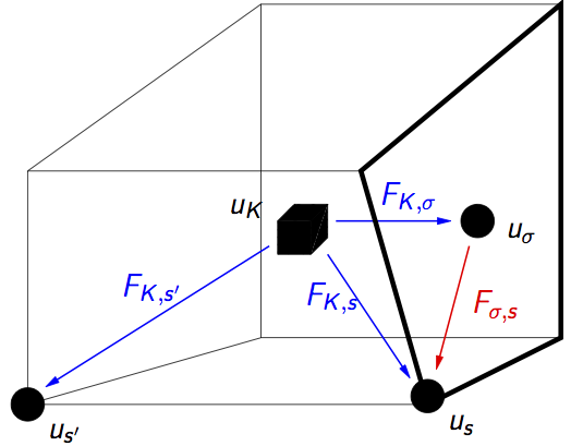
Figure 2: For a cell $K$ and a fracture face $\sigma$ (in bold), examples of VAG degrees of freedom $u_{K}$, $u_{\bf s}$, $u_{\sigma}$, $u_{{\bf s}^{\prime}}$ and VAG fluxes $F_{K,\sigma}$, $F_{K,{\bf s}}$, $F_{K,{\bf s}^{\prime}}$, $F_{\sigma,{\bf s}}$.

The construction of the control volumes at each degree of freedom is based on partitions of the cells and of the fracture faces. These partitions are respectively denoted, for all $K\in{\cal M}$, by

$$\overline{K}~{}=~{}\overline{\omega}_{K}~{}\bigcup~{}\left(\bigcup_{{\bf s}\in{\cal V}_{K}\setminus({\cal V}_{D}\cup{\cal V}_{\Gamma})}\overline{\omega}_{K,{\bf s}}\right),$$

and, for all $\sigma\in{\cal F}_{\Gamma}$, by

$$\overline{\sigma}~{}=~{}\overline{\Sigma}_{\sigma}~{}\bigcup~{}\left(\bigcup_{{\bf s}\in{\cal V}_{\sigma}\setminus{\cal V}_{D}}\overline{\Sigma}_{\sigma,{\bf s}}\right).$$

It is important to notice that in the usual case of cellwise constant rocktypes in the matrix and facewise constant rocktypes in the fracture network, the implementation of the scheme does not require to build explicitly the geometry of these partitions. In that case, it is sufficient to define the matrix volume fractions

$$\alpha_{K,{\bf s}}={\int_{\omega_{K,{\bf s}}}d{\bf x}\over\int_{K}d{\bf x}},{\bf s}\in{\cal V}_{K}\setminus({\cal V}_{D}\cup{\cal V}_{\Gamma}),K\in{\cal M},$$

constrained to satisfy $\alpha_{K,{\bf s}}\geq 0$, and $\sum_{{\bf s}\in{\cal V}_{K}\setminus({\cal V}_{D}\cup{\cal V}_{\Gamma})}\alpha_{K,{\bf s}}\leq 1$, as well as the fracture volume fractions

$$\alpha_{\sigma,{\bf s}}={\int_{\Sigma_{\sigma,{\bf s}}}d_{f}({\bf x})d\tau({\bf x})\over\int_{\sigma}d_{f}({\bf x})d\tau({\bf x})},{\bf s}\in{\cal V}_{\sigma}\setminus{\cal V}_{D},\sigma\in{\cal F}_{\Gamma},$$

constrained to satisfy $\alpha_{\sigma,{\bf s}}\geq 0$, and $\sum_{{\bf s}\in{\cal V}_{\sigma}\setminus{\cal V}_{D}}\alpha_{\sigma,{\bf s}}\leq 1$, where we denote by $d\tau({\bf x})$ the $2$ dimensional Lebesgue measure on $\Gamma$. Let us also set

$$\phi_{K}=(1-\sum_{{\bf s}\in{\cal V}_{K}\setminus({\cal V}_{D}\cup{\cal V}_{\Gamma})}\alpha_{K,{\bf s}})\int_{K}\phi_{m}({\bf x})d{\bf x}\quad\mbox{ for }K\in{\cal M},$$

and

$$\phi_{\sigma}=(1-\sum_{{\bf s}\in{\cal V}_{\sigma}\setminus{\cal V}_{D}}\alpha_{\sigma,{\bf s}})\int_{\sigma}\phi_{f}({\bf x})d_{f}({\bf x})d\tau({\bf x})\quad\mbox{ for }\sigma\in{\cal F}_{\Gamma},$$

as well as

$$\phi_{{\bf s}}=\sum_{K\in{\cal M}_{\bf s}}\alpha_{K,{\bf s}}\int_{K}\phi_{m}({\bf x})d{\bf x}\quad\mbox{ for }{\bf s}\in{\cal V}\setminus({\cal V}_{D}\cup{\cal V}_{\Gamma}),$$

and

$$\phi_{{\bf s}}=\sum_{\sigma\in{\cal F}_{\Gamma,{\bf s}}}\alpha_{\sigma,{\bf s}}\int_{\sigma}\phi_{f}({\bf x})d_{f}({\bf x})d\tau({\bf x})\quad\mbox{ for }{\bf s}\in{\cal V}_{\Gamma}\setminus{\cal V}_{D},$$

which correspond to the porous volume distributed to the degrees of freedom excluding the Dirichlet nodes. The rock complementary volumes in each control volume $\nu\in{\cal M}\cup{\cal F}_{\Gamma}\cup({\cal V}\setminus{\cal V}_{D})$ are denoted by $\bar{\phi}_{\nu}$.

As shown in [13], the flexibility in the choice of the control volumes is a crucial asset, compared with usual CVFE approaches and allows to significantly improve the accuracy of the scheme when the permeability field is highly heterogeneous. As exhibited in Figure 3, as opposed to usual CVFE approaches, this flexibility allows to define the control volumes in the fractures with no contribution from the matrix in order to avoid to enlarge artificially the flow path in the fractures.

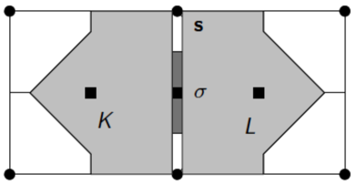
Figure 3: Two cells $K$ and $L$ splitted by one fracture face $\sigma$ in red in the left figure. In the right figure, example of control volumes at the two cells $K$ and $L$, at the fracture face $\sigma$, and at nodes (the width of the fracture is enlarged in the right figure). The control volumes are chosen to avoid to mix the fracture and matrix porous volumes.

In the following, we will keep the notation $F_{K,s}$, $F_{K,\sigma}$, $F_{\sigma,s}$ for the VAG Darcy fluxes defined with the cellwise constant matrix permeability ${\bf K}_{m}$ and the facewise constant fracture width $d_{f}$ and tangential permeability ${\bf K}_{f}$. Since the rock properties are fixed, the VAG Darcy fluxes transmissibility matrices $T_{K}$ and $T_{\sigma}$ are computed only once.

The VAG Fourier fluxes are denoted in the following by $G_{K,{\bf s}}$, $G_{K,\sigma}$, $G_{\sigma,{\bf s}}$. They are obtained with the isotropic matrix and fracture thermal conductivities averaged in each cell and in each fracture face using the previous time step fluid properties. Hence VAG Fourier fluxes transmissibility matrices need to be recomputed at each time step.

3.2 VAG discretization of the hybrid-dimensional non-isothermal compositional model

The time integration is based on a fully implicit Euler scheme to avoid severe restrictions on the time steps due to the small volumes and high velocities in the fractures. Note that the thermal conductivities are discretized as mentioned above using the saturations at the previous time step. A phase based upwind scheme is used for the approximation of the mobilities in the Darcy fluxes, that is to say the same scheme that is already used in the definition of the transmission conditions (15) of the hybrid-dimensional model. At the matrix fracture interfaces, we avoid the mixing of the matrix and fracture rocktypes in our choice of the control volumes for $\sigma\in{\cal F}_{\Gamma}$ and ${\bf s}\in{\cal V}_{\Gamma}$ (see Figure 3). To avoid too small control volumes at the nodes ${\bf s}\in{\cal V}_{\Sigma}$ located at the fracture intersection, the volume is distributed to such a node ${\bf s}$ from all the fracture faces containing the node ${\bf s}$. It results that the volumes of the control volumes ${\bf s}\in{\cal V}_{\Sigma}$ at the fracture intersection is not smaller than at any other matrix fracture degrees of freedom. This solves the problems reported in [4] and [17] related to the small volumes at the fracture intersections and avoid the Star-Delta transformation used in [4] which is not valid in the case of multiphase flows.

For $N_{T}\in\mathbb{N}^{*}$, let us consider the time discretization $t^{0}=0<t^{1}<\cdots<t^{n-1}<t^{n}\cdots<t^{N_{T}}=T$ of the time interval $[0,T]$. We denote the time steps by $\Delta t^{n}=t^{n}-t^{n-1}$ for all $n=1,\cdots,N_{T}$.

Let be given, for each degree of freedom $\nu\in{\cal M}\cup{\cal F}_{\Gamma}\cup{\cal V}$, the set of physical unknowns of the Coats’ formulation

$$X_{\nu}=\Bigl{(}P_{\nu},T_{\nu},S_{\nu}^{\alpha},C_{\nu}^{\alpha},\alpha\in Q_{\nu},n_{i,\nu},i\in\overline{\cal C}_{Q_{\nu}},Q_{\nu}\Bigr{)}.$$

We denote by $X_{\cal D}$, the full set of unknowns

$$X_{\cal D}=\{X_{\nu},\nu\in{\cal M}\cup{\cal F}_{\Gamma}\cup{\cal V}\}.$$

We will use the notation $Q_{\cal D}=\Bigl{(}Q_{\nu},\nu\in{\cal M}\cup{\cal F}_{\Gamma}\cup{\cal V}\Bigr{)}$, and, for a given $Q_{\nu}$, we denote by

$$X_{Q_{\nu}}=\Bigl{(}P_{\nu},T_{\nu},S_{\nu}^{\alpha},C_{\nu}^{\alpha},\alpha\in Q_{\nu},n_{i,\nu},i\in\overline{\cal C}_{Q_{\nu}}\Bigr{)},$$

the set of physical unknowns excluding the set of present phases $Q_{\nu}$. Similarly, for a given $Q_{\cal D}$, we set

$$X_{Q_{\cal D}}=\{X_{Q_{\nu}},\nu\in{\cal M}\cup{\cal F}_{\Gamma}\cup{\cal V}\}.$$

We can clearly identify $X_{\nu}$ and $(X_{Q_{\nu}},Q_{\nu})$ as well as $X_{\cal D}$ and $(X_{Q_{\cal D}},Q_{\cal D})$.

The Darcy fluxes taking into account the gravity term are defined by

$$\left\{\begin{array}[]{r@{\,\,}c@{\,\,}ll}&V^{\alpha}_{K,\nu}(X_{\cal D})&=&F_{K,\nu}(P_{\cal D})+\rho_{K,\nu}^{\alpha}F_{K,\nu}({\cal G}_{\cal D}),\,\,\nu\in\Xi_{K},K\in{\cal M},\\ &V^{\alpha}_{\sigma,{\bf s}}(X_{\cal D})&=&F_{\sigma,{\bf s}}(P_{\cal D})+\rho_{\sigma,s}^{\alpha}F_{\sigma,{\bf s}}({\cal G}_{\cal D}),\,\,{\bf s}\in{\cal V}_{\sigma},\sigma\in{\cal F}_{\Gamma},\end{array}\right.$$ (17)

where ${\cal G}_{\cal D}$ denotes the vector $({\bf g}\cdot{\bf x}_{\nu})_{\nu\in{\cal M}\cup{\cal F}_{\Gamma}\cup{\cal V}}$, and the phase mass density is defined by the weighted average

$$\rho_{\nu,\nu^{\prime}}^{\alpha}={S^{\alpha}_{\nu}\rho^{\alpha}(P_{\nu},T_{\nu},C^{\alpha}_{\nu})+S^{\alpha}_{\nu^{\prime}}\rho^{\alpha}(P_{\nu^{\prime}},T_{\nu^{\prime}},C^{\alpha}_{\nu^{\prime}})\over S^{\alpha}_{\nu}+S^{\alpha}_{\nu^{\prime}}}.$$

The discretization of the mobilities is obtained using a usual phase based upwinding (see e.g. [37]). For each Darcy flux, let us define the phase dependent upwind control volume $cv_{\mu,\nu}^{\alpha}$ such that

$$cv_{K,\nu}^{\alpha}=\left\{\begin{array}[]{r@{\,\,}c@{\,\,}l}K&\text{ if }&V^{\alpha}_{K,{\nu}}(X_{\cal D})\geqslant 0\\ \nu&\text{ if }&V^{\alpha}_{K,{\nu}}(X_{\cal D})<0\end{array}\right.\text{ for }K\in{\cal M},\nu\in\Xi_{K},$$

for the matrix fluxes, and such that

$$cv_{\sigma,s}^{\alpha}=\left\{\begin{array}[]{r@{\,\,}c@{\,\,}l}\sigma&\text{ if }&V^{\alpha}_{\sigma,s}(X_{\cal D})\geqslant 0\\ s&\text{ if }&V^{\alpha}_{\sigma,s}(X_{\cal D})<0\end{array}\right.\text{ for }\sigma\in{\cal F}_{\Gamma},s\in{\cal V}_{\sigma},$$

for fracture fluxes. Using this upwind discretization, the component molar fluxes are given by

$$q_{i,\nu,\nu^{\prime}}(X_{\cal D})=\sum_{\alpha\in Q_{cv_{\nu,\nu^{\prime}}^{\alpha}}\cap\mathcal{P}_{i}}m_{i}^{\alpha}(X_{cv_{\nu,\nu^{\prime}}^{\alpha}})V^{\alpha}_{\nu,\nu^{\prime}}(X_{\cal D})$$

for $i\in{\cal C}$, and the energy fluxes by

$$q_{e,\nu,\nu^{\prime}}(X_{\cal D})=\sum_{\alpha\in Q_{cv_{\nu,\nu^{\prime}}^{\alpha}}\cap\mathcal{P}_{i}}m_{e}^{\alpha}(X_{cv_{\nu,\nu^{\prime}}^{\alpha}})V^{\alpha}_{\nu,\nu^{\prime}}(X_{\cal D})+G_{\nu,\nu^{\prime}}(T_{\cal D}).$$

Next, in each control volume $\nu$, let us denote by

$${\cal A}_{i,\nu}(X_{\nu})=\phi_{\nu}n_{i}(X_{\nu}),\ i\in{\cal C}$$

the component molar accumulation, and by

$${\cal A}_{e,\nu}(X_{\nu})=\phi_{\nu}E(X_{\nu})+\bar{\phi}_{\nu}E_{r}(P_{\nu},T_{\nu}),$$

the energy accumulation.

We can now state the system of discrete equations at each time step $n=1,\cdots,N_{T}$ which accounts for the component and energy conservation equations $i\in{\cal C}\cup\{e\}$ in each cell $K\in{\cal M}$

$$R_{K,i}(X_{\cal D}^{n}):=\frac{{\cal A}_{i}(X_{K}^{n})-{\cal A}_{i}(X_{K}^{n-1})}{\Delta t^{n}}+\sum_{{\bf s}\in{\cal V}_{K}}q_{i,K,{\bf s}}(X_{\cal D}^{n})+\sum_{\sigma\in{\cal F}_{\Gamma}\cap{\cal F}_{K}}q_{i,K,\sigma}(X_{\cal D}^{n})=0,$$ (18)

in each fracture face $\sigma\in{\cal F}_{\Gamma}$

$$R_{\sigma,i}(X_{\cal D}^{n}):=\frac{{\cal A}_{i}(X_{\sigma}^{n})-{\cal A}_{i}(X_{\sigma}^{n-1})}{\Delta t^{n}}+\sum_{{\bf s}\in{\cal V}_{\sigma}}q_{i,\sigma,{\bf s}}(X_{\cal D}^{n})+\sum_{K\in{\cal M}_{\sigma}}-q_{i,K,\sigma}(X_{\cal D}^{n})=0,$$ (19)

and at each node ${\bf s}\in{\cal V}\setminus{\cal V}_{D}$

$$R_{s,i}(X_{\cal D}^{n}):=\frac{{\cal A}_{i}(X_{\bf s}^{n})-{\cal A}_{i}(X_{\bf s}^{n-1})}{\Delta t^{n}}+\sum_{\sigma\in{\cal F}_{\Gamma,{\bf s}}}-q_{i,\sigma,{\bf s}}(X_{\cal D}^{n})+\sum_{K\in{\cal M}_{\bf s}}-q_{i,K,{\bf s}}(X_{\cal D}^{n})=0.$$ (20)

It is coupled with the local closure laws

$$\mathbf{0}=L_{\nu}(X_{\nu}^{n}):=\left\{\begin{array}[]{l}\displaystyle{\sum_{\alpha\in Q_{\nu}^{n}}S^{\alpha,n}_{\nu}}-1,\\ \displaystyle{\sum_{i\in{\cal C}^{\alpha}}C_{i,\nu}^{\alpha,n}}-1,\,\,\alpha\in Q^{n}_{\nu},\\ f_{i}^{\alpha}(P^{n}_{\nu},T_{\nu}^{n},C_{\nu}^{\alpha,n})C_{i,\nu}^{\alpha,n}-f_{i}^{\beta}(P^{n}_{\nu},T_{\nu}^{n},C_{\nu}^{\beta,n})C_{i,\nu}^{\beta,n},\\ \quad\quad\quad\quad\quad\alpha\neq\beta,(\alpha,\beta)\in(Q^{n}_{\nu}\cap{\cal P}_{i})^{2}.\,\,i\in{\cal C},\end{array}\right.$$ (21)

the flash computations $Q^{n}_{\nu}=Q_{flash}(X^{n}_{\nu})$ for $\nu\in{\cal M}\cup({\cal V}\setminus{\cal V}_{\cal D})\cup{\cal F}_{\Gamma}$, and the Dirichlet boundary conditions

$$X_{\bf s}=X_{{\bf s},D},$$

for all ${\bf s}\in{\cal V}_{\cal D}$.

3.3 Newton-Raphson non-linear solver

Let us denote by $R_{\nu}(X_{\cal D})$ the vector $\Bigl{(}R_{\nu,i},\ i\in\mathcal{C}\cup\{e\}\Bigr{)}$, and let us rewrite the conservation equations (18), (19), (20) and the closure laws (21) as well as the boundary conditions in vector form defining the following non-linear system at each time step $n=1,2,...,N_{T}$

$$\mathbf{0}=\mathcal{R}(X_{\cal D}):=\left\{\begin{array}[]{llllll}\left(\begin{array}[]{c}R_{{\bf s}}(X_{\cal D})\\ L_{\bf s}(X_{s})\end{array}\right)\ {\bf s}\in{\cal V},\\ \left(\begin{array}[]{c}R_{\sigma}(X_{\cal D})\\ L_{\sigma}(X_{\sigma})\end{array}\right)\ \sigma\in{\cal F}_{\Gamma},\\ \left(\begin{array}[]{c}R_{K}(X_{\cal D})\\ L_{K}(X_{K})\end{array}\right)\ K\in{\cal M},\end{array}\right.$$ (31)

where the superscript $n$ is dropped to simplify the notations and where the Dirichlet boundary conditions have been included at each Dirichlet node ${\bf s}\in{\cal V}_{D}$ in order to obtain a system size independent on the boundary conditions.

The non-linear system ${\cal R}(X_{\cal D})=0$ coupled to the flash fixed point equations $Q_{\nu}=Q_{flash}(X_{\nu})$, $\nu\in{\cal M}\cup{\cal F}_{\Gamma}\cup({\cal V}\setminus{\cal V}_{D})$ is solved by an active set Newton-Raphson algorithm widely used in the reservoir simulation community [33] which is detailed below. The algorithm is initialized with an initial guess $X_{Q_{\cal D}}^{(0)}$,$Q_{{\cal D}}^{(0)}$ usually given by the previous time step solution and computes the initial residual $\mathcal{R}(X_{Q_{\cal D}}^{(0)},Q_{{\cal D}}^{(0)})$ and its norm $||\mathcal{R}(X_{Q_{\cal D}}^{(0)},Q_{{\cal D}}^{(0)})||$ for a given weighted norm $\|.\|$.

The Newton algorithm iterates on the following steps for $r=0,\cdots,$ until convergence of the relative residual

$${||\mathcal{R}(X_{Q_{\cal D}}^{(r)},Q_{{\cal D}}^{(r)})||\over||\mathcal{R}(X_{Q_{\cal D}}^{(0)},Q_{{\cal D}}^{(0)})||}\leq\epsilon_{newton}$$

for a given stopping criteria $\epsilon_{newton}$ or until it reaches a maximum number of Newton steps $N_{newton}^{max}$.

1. Computation of the Jacobian matrix

   $$J^{(r)}={\partial{\cal R}\over\partial X_{{Q_{\cal D}}}}\Big{(}X_{{Q_{\cal D}}}^{(r)},Q^{(r)}_{{{\cal D}}}\Big{)}.$$

2. Solution of the linear system

   $$J^{(r)}~{}dX^{(r)}_{{Q_{\cal D}}}=-{\cal R}\Big{(}X_{{Q_{\cal D}}}^{(r)},Q^{(r)}_{{{\cal D}}}\Big{)}.$$ (32)

3. Update of the unknowns $X_{{Q_{\cal D}}}^{(r)}$ with a full Newton step $\theta^{(r)}=1$ or a possible relaxation $\theta^{(r)}\in(0,1)$.

   $$X_{{Q_{\cal D}}}^{(r+{1\over 2})}=X_{{Q_{\cal D}}}^{(r)}+\theta^{(r)}~{}dX^{(r)}_{{Q_{\cal D}}}.$$

4. Flash computations to update the sets of present phases $Q_{{{\cal D}}}^{(r+1)}$. The flash computations also provide the molar fractions of the new sets of present phases. They are used together with $X_{Q_{\cal D}}^{(r+{1\over 2})}$ and $Q_{{\cal D}}^{(r+1)}$ to update the new set of unknowns $X_{Q_{\cal D}}^{(r+1)}$.

5. Computation of the new residual $\mathcal{R}(X_{Q_{\cal D}}^{(r+1)},Q_{{\cal D}}^{(r+1)})$ and of its norm.

If the Newton algorithm reaches the predefined maximum number of iterations before convergence, then we restart this time step with a reduced $\Delta t$.

In view of the non-linear system (31), the size of the linear system for the computation of the Newton step can be considerably reduced without fill-in by

• Step 1: elimination of the local closure laws (21),

• Step 2: elimination of the cell unknowns.

Step 2 is detailed in Section 4.2. The elimination of the local closure laws (Step 1) is achieved for each control volume $\nu\in{\mathcal{M}\cup\mathcal{F}_{\Gamma}\cup\mathcal{V}}$ by splitting the unknowns $X_{Q_{\nu}}$ into $\#{\cal C}+1$ primary unknowns $X_{Q_{\nu}}^{pr}$ and $N^{sd}_{\nu}$ secondary unknowns $X_{Q_{\nu}}^{sd}$ with

$$N^{sd}_{\nu}=1+\#Q_{\nu}+\sum_{\alpha\in Q_{\nu}}\#{\cal C}^{\alpha}+\#\overline{\cal C}_{Q_{\nu}}-\#{\cal C}.$$

For each control volume $\nu\in{\mathcal{M}\cup\mathcal{F}_{\Gamma}\cup\mathcal{V}}$, the secondary unknowns are chosen in such a way that the square matrix

$${\partial L\over\partial X^{sd}_{Q_{\nu}}}\left(X^{pr}_{Q_{\nu}},X_{Q_{\nu}}^{sd},Q_{\nu}\right)\in\mathbb{R}^{N^{sd}_{\nu}\times N^{sd}_{\nu}},$$

is non-singular. This choice can be done algebraically in the general case, or defined once and for all for each set of present phases $Q_{\nu}$ for specific physical cases. Here we remark that the unknowns $(n_{i,\nu})_{i\in\overline{\cal C}_{Q_{\nu}}}$ are not involved in the closure laws (21) and hence are always chosen as primary unknowns.

The ill conditioned linear system obtained from (32) after the two elimination steps is solved using an iterative solver such as GMRES or BiCGStab combined with a preconditioner adapted to the elliptic or parabolic nature of the pressure unknown and to the coupling with the remaining hyperbolic or parabolic unknowns. One of the most efficient preconditioners for such systems is the so-called CPR-AMG preconditioner introduced in [35] and [36]. It combines multiplicatively an algebraic multigrid preconditioner (AMG) for a pressure block of the linear system [39] with a more local preconditioner for the full system, such as an incomplete LU factorization. The choice of the pressure block is important for the efficiency of the CPR-AMG preconditioner. In the following experiments we simply define the pressure equation in each control volume by the sum of the molar conservation equations in the control volume. Let us refer to [35], [36], and [40] for a discussion on other possible choices. Let us denote by $Jx=b$ the linear system where $J$ is the Jacobian matrix and $b$ the right hand side taking into account the elimination steps and the linear combinations of the lines for the pressure block. The CPR-AMG preconditioner $\mathcal{P}_{\mathrm{cpr-amg}}$ is defined for any vector $b$ by $\mathcal{P}_{\mathrm{cpr-amg}}b=v$ with

$$v^{1/2}=R_{P}^{\top}\mathcal{P}_{\mathrm{amg}(J_{P})}R_{P}b,$$

$$v=v^{1/2}+\mathcal{P}_{\mathrm{ilu0}}(b-Jv^{1/2}),$$ (33)

where $\mathcal{P}_{\mathrm{amg}(J_{P})}$ is the AMG preconditioner with $J_{P}=R_{P}JR_{P}^{\top}$, $\mathcal{P}_{\mathrm{ilu0}}$ is the ILU(0) preconditioner applied on the Jacobian $J$, $R_{P}$ is the restriction matrix to the pressure unknowns and $R_{P}^{\top}$ is the transpose of $R_{P}$.

4 Parallel implementation

Parallel implementation is achieved using the Message Passing Interface (MPI). Let us denote by $N_{p}$ the number of MPI processes.

4.1 Mesh decomposition

The set of cells ${\cal M}$ is partitioned into $N_{p}$ subsets ${\cal M}^{p},p=1,...,N_{p}$ using the library METIS [41]. In the current implementation, this partitioning is only based on the cell connectivity graph and does not take into account the fracture faces. This will be investigated in the near future and the potential gain is discussed in the numerical section. The partitioning of the set of nodes $\mathcal{V}$ and of the set of fracture faces $\mathcal{F}_{\Gamma}$ is defined as follows: assuming we have defined a global index of the cells $K\in{\cal M}$ let us denote by $K({\bf s}),{\bf s}\in{\cal V}$ (resp. $K(\sigma)$, $\sigma\in{\cal F}_{\Gamma}$) the cell with the smallest global index among those of ${\cal M}_{\bf s}$ (resp. ${\cal M}_{\sigma}$). Then we set

$${\cal V}^{p}=\{{\bf s}\in{\cal V}\,|\,K({\bf s})\in{\cal M}^{p}\},$$

and

$${\cal F}_{\Gamma}^{p}=\{\sigma\in{\cal F}_{\Gamma}\,|\,K(\sigma)\in{\cal M}^{p}\}.$$

The overlapping decomposition of ${\cal M}$ into the sets

$$\overline{{\cal M}}^{p},\,\,p=1,...,N_{p},$$

is chosen in such a way that any compact finite volume scheme such as the VAG scheme can be assembled locally on each process. Hence, as exhibited in Figure 4, $\overline{{\cal M}}^{p}$ is defined as the set of cells sharing a node with a cell of ${\cal M}^{p}$. The overlapping decompositions of the set of nodes and of the set of fracture faces follow from this definition:

$$\overline{\cal V}^{p}=\bigcup_{K\in\overline{\cal M}^{p}}{\cal V}_{K},\,\,p=1,\cdots,N_{p},$$

and

$$\overline{\cal F}_{\Gamma}^{p}=\bigcup_{K\in\overline{\cal M}^{p}}{\cal F}_{K}\cap{\cal F}_{\Gamma},\,\,p=1,\cdots,N_{p}.$$

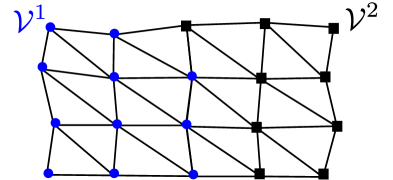
Figure 4: Example of mesh decomposition.

The partitioning of the mesh is performed by the master process (process 1), and then, each local mesh is distributed to its process. Therefore, each MPI process contains the local mesh ($\overline{{\cal M}}^{p}$, $\overline{\cal V}^{p}$, $\overline{\cal F}_{\Gamma}^{p}$), $p=1,2,...,N_{p}$ which is splitted into two parts:

$$\begin{split}&\text{own mesh: }({\cal M}^{p},{\cal V}^{p},{\cal F}_{\Gamma}^{p}),\\ &\text{ghost mesh: }(\overline{{\cal M}}^{p}\backslash{\cal M}^{p},\overline{\cal V}^{p}\backslash{\cal V}^{p},\overline{\cal F}_{\Gamma}^{p}\backslash{\cal F}_{\Gamma}^{p}).\end{split}$$

We now turn to the parallel implementation of the Jacobian system.

4.2 Parallelization of the Jacobian system

On each process $p=1,...,N_{p}$, the local Jacobian system is defined by the set of unknowns $X_{\nu}$, $\nu\in\overline{\cal V}^{p}\cup\overline{\cal F}_{\Gamma}^{p}\cup\overline{\cal M}^{p}$, the closure equations on control volume $\nu\in\overline{\cal V}^{p}\cup\overline{\cal F}_{\Gamma}^{p}\cup\overline{\cal M}^{p}$ and the conservation equations of all own nodes ${\bf s}\in\mathcal{V}^{p}$, all own fracture faces $\sigma\in\mathcal{F}_{\Gamma}^{p}$ and all own and ghost cells $k\in\overline{{\cal M}}^{p}$.

The local Jacobian system is firstly reduced by eliminating the local closure laws on each control volume $\nu\in\overline{\cal V}^{p}\cup\overline{\cal F}_{\Gamma}^{p}\cup\overline{\cal M}^{p}$ using the procedure presented in Section 3.3. The local reduced Jacobian system can be written as the following rectangular linear system

$$\begin{pmatrix}J_{ss}^{p}&J_{sf}^{p}&J_{sc}^{p}\\ J_{fs}^{p}&J_{ff}^{p}&J_{fc}^{p}\\ J_{cs}^{p}&J_{cf}^{p}&J_{cc}^{p}\end{pmatrix}\begin{pmatrix}\overline{U}_{s}^{p}\\ \overline{U}_{f}^{p}\\ \overline{U}_{c}^{p}\end{pmatrix}=\begin{pmatrix}b_{s}^{p}\\ b_{f}^{p}\\ b_{c}^{p}\end{pmatrix}$$

where $\overline{U}_{s}^{p}\in\mathbb{R}^{\#\overline{\mathcal{V}}^{p}\times(\#\mathcal{C}+1)}$, $\overline{U}_{f}^{p}\in\mathbb{R}^{\#\overline{\mathcal{F}}_{\Gamma}^{p}\times(\#\mathcal{C}+1)}$ and $\overline{U}_{c}^{p}\in\mathbb{R}^{\#\overline{{\cal M}}^{p}\times(\#\mathcal{C}+1)}$ denote the vector of own and ghost primary unknowns $X^{pr}_{Q_{\nu}}$ at the nodes $\nu\in{\overline{\cal V}}^{p}$, at the fracture faces $\nu\in{\overline{\cal F}}_{\Gamma}^{p}$ and at the cells $\nu\in{\overline{\cal M}}^{p}$ respectively on the process $p$. The above matrices have the following sizes

$$J_{ss}^{p}\in\mathbb{R}^{\big{(}\#\mathcal{V}^{p}\times(\#\mathcal{C}+1)\big{)}\times\big{(}\#\overline{\mathcal{V}}^{p}\times(\#\mathcal{C}+1)\big{)}},$$

$$J_{ff}^{p}\in\mathbb{R}^{\big{(}\#\mathcal{F}_{\Gamma}^{p}\times(\#\mathcal{C}+1)\big{)}\times\big{(}\#\overline{\mathcal{F}}_{\Gamma}^{p}\times(\#\mathcal{C}+1)\big{)}},$$

$$J_{cc}^{p}\in\mathbb{R}^{\big{(}\#\overline{{\cal M}}^{p}\times(\#\mathcal{C}+1)\big{)}\times\big{(}\#\overline{{\cal M}}^{p}\times(\#\mathcal{C}+1)\big{)}},$$

and $b_{s}^{p}\in\mathbb{R}^{\#{\mathcal{V}}^{p}\times(\#\mathcal{C}+1)}$, $b_{f}^{p}\in\mathbb{R}^{\#{\mathcal{F}}_{\Gamma}^{p}\times(\#\mathcal{C}+1)}$ and $b_{c}^{p}\in\mathbb{R}^{\#\overline{{\cal M}}^{p}\times(\#\mathcal{C}+1)}$ denote the corresponding right hand side vectors. The matrix $J_{cc}^{p}$ is a non singular diagonal matrix and the cell unknowns can be easily eliminated without fill-in leading to the following Schur complement system

$$J^{p}\begin{pmatrix}\overline{U}_{s}^{p}\\ \overline{U}_{f}^{p}\end{pmatrix}=b^{p},$$ (34)

with

$$\begin{split}&J^{p}:=\begin{pmatrix}J_{ss}^{p}&J_{sf}^{p}\\ J_{fs}^{p}&J_{ff}^{p}\end{pmatrix}-\begin{pmatrix}J_{sc}^{p}\\ J_{fc}^{p}\end{pmatrix}(J_{cc}^{p})^{-1}\begin{pmatrix}J_{cs}^{p}&J_{cf}^{p}\end{pmatrix},\\ &b^{p}:=\begin{pmatrix}b_{s}^{p}\\ b_{f}^{p}\end{pmatrix}-\begin{pmatrix}J_{sc}^{p}\\ J_{fc}^{p}\end{pmatrix}(J_{cc}^{p})^{-1}b_{c}^{p},\end{split}$$

and

$$\overline{U}_{c}^{p}=(J_{cc}^{p})^{-1}(b_{c}^{p}-J_{cs}^{p}\overline{U}_{s}^{p}-J_{cf}^{p}\overline{U}_{f}^{p}).$$ (35)

The linear system (34) is built locally on each process $p$ and transfered to the parallel linear solver library PETSc [42]. The parallel matrix and the parallel vector in PETSc are stored in a distributed manner, i.e. each process stores its own rows. We construct the following parallel global linear system

$$JU=b,$$ (36)

with

$$J:=\begin{pmatrix}J^{1}R^{1}\\ J^{2}R^{2}\\ \vdots\\ J^{N_{p}}R^{N_{p}}\end{pmatrix}\begin{array}[]{l}\big{\}}\text{ process 1}\\ \big{\}}\text{ process 2}\\ \quad\quad\vdots\\ \big{\}}\text{ process $N_{p}$}\end{array},$$

and

$$U:=\begin{pmatrix}U_{s}^{1}\\ U_{f}^{1}\\ U_{s}^{2}\\ U_{f}^{2}\\ \vdots\\ U_{s}^{N_{p}}\\ U_{f}^{N_{p}}\end{pmatrix}\begin{array}[]{l}\bigg{\}}\text{ process 1}\\ \bigg{\}}\text{ process 2}\\ \quad\quad\vdots\\ \bigg{\}}\text{ process $N_{p}$}\end{array},\ b:=\begin{pmatrix}b^{1}\\ b^{2}\\ \vdots\\ b^{N_{p}}\end{pmatrix}\begin{array}[]{l}\big{\}}\text{ process 1 }\\ \big{\}}\text{ process 2 }\\ \quad\quad\vdots\\ \big{\}}\text{ process $N_{p}$}\end{array}$$

where $R^{p},p=1,2,...,N_{p}$ is a restriction matrix satisfying

$$R^{p}U=\begin{pmatrix}\overline{U}_{s}^{p}\\ \overline{U}_{f}^{p}\end{pmatrix}.$$

The matrix $J^{p}R^{p}$, the vector $\begin{pmatrix}U_{s}^{p}\\ U_{f}^{p}\end{pmatrix}$ and the vector $b^{p}$ are stored in process $p$.

The linear system (36) is solved using the GMRES algorithm preconditioned by CPR-AMG preconditioner as discussed in the previous section. The solution of the linear system provides on each process $p$ the solution vector $\begin{pmatrix}U_{s}^{p}\\ U_{f}^{p}\end{pmatrix}$ of own node and fracture-face unknowns. Then, the ghost node unknowns $U^{p}_{\nu}$, $\nu\in(\overline{\cal V}^{p}\backslash{\cal V}^{p})$ and the ghost fracture face unknowns $U_{\nu}^{p}$, $\nu\in(\overline{\cal F}_{\Gamma}^{p}\backslash{\cal F}_{\Gamma}^{p})$ are recovered by a synchronization step with MPI communications. This synchronization is efficiently implemented using a PETSc matrix vector product

$$\overline{U}=SU$$ (37)

where

$$\overline{U}:=\begin{pmatrix}\overline{U}_{s}^{1}\\ \overline{U}_{f}^{1}\\ \overline{U}_{s}^{2}\\ \overline{U}_{f}^{2}\\ \vdots\end{pmatrix}$$

is the vector of own and ghost node and fracture-face unknowns on all processes. The matrix $S$, containing only $0$ and $1$ entries, is assembled once and for all at the beginning of the simulation.

Finally, thanks to (35), the vector of own and ghost cell unknowns $\overline{U}_{c}^{p}$ is computed locally on each process $p$.

5 Numerical results

The numerical tests are all implemented in the framework of the code ComPASS on the cluster “cicada” hosted by University Nice Sophia-Antipolis consisting of 72 nodes (16 cores/node, Intel Sandy Bridge E5-2670, 64GB/node). We always fix 1 core per process and 16 processes per node. The communications are handled by OpenMPI 1.8.2 (GCC 4.9).

Five test cases are considered in the following subsections. They include a two-phase immiscible isothermal Darcy flow model, a two-phase isothermal Black Oil model and a non-isothermal liquid gas flow model. Different types of meshes namely hexahedral, tetrahedral, prismatic and Cartesian meshes are used in these simulations.

The settings of the nonlinear Newton and linear GMRES solvers are defined by their maximum number of iterations denoted by $N_{newton}^{max}$ and $N_{gmres}^{max}$ and by their stopping criteria on the relative residuals denoted by $\epsilon_{newton}$ and $\epsilon_{gmres}$.

The time stepping is defined by an initial time step $\Delta t^{(0)}$ and by a maximum time step $\Delta t^{(k)}$ on each time interval $[t^{(k)},t^{(k+1)})$, $k=0,\cdots,k_{f}-1$ with $t^{(0)}=0$ and $t^{(k_{f})}=t_{f}$, where $t_{f}$ is the final simulation time. The successive time steps are computed using the following rules. If the Newton algorithm reaches convergence in less than $N_{newton}^{max}$ iterations at time step $n$ with $t^{n}\in[t^{(k)},t^{(k+1)})$, then the next time step $\Delta t^{n+1}$ is set to

$$\Delta t^{n+1}=\mathrm{min}(c\Delta t^{n},\Delta t^{(k)}),\ c=1.2.$$ (38)

If the Newton algorithm does not converge in $N_{newton}^{max}$ iterations or if the linear solver does not reach convergence in $N_{gmres}^{max}$ iterations, then the time step is chopped by a factor two and restarted.

In all the following numerical experiments, the relative permeabilities are given by the Corey laws $k_{r}^{\alpha}(S)=(S^{\alpha})^{2}$ for both phases $\alpha\in\mathcal{P}$ and both in the matrix domain and in the fracture network.

5.1 Two-phase immiscible isothermal flow

In this subsection, we consider an immiscible isothermal two-phase Darcy flow with $\mathcal{P}=\{\mathrm{water,oil}\}$ the set of phases and $\mathcal{C}=\{H_{2}O,HC\}$ the set of components. The model prescribes the mass conservation and we set $\rho^{water}=1000\text{ kg/m${}^{3}$}$ and $\rho^{oil}=700\text{ kg/m${}^{3}$}$. The phase viscosities are set to $\mu^{water}=10^{-3}$ $\text{Pa}\cdot\text{s}$ and $\mu^{oil}=5.0\times 10^{-3}$ $\text{Pa}\cdot\text{s}$.

The reservoir domain is defined by $\Omega=(0,100)^{3}$ in meter. We consider a topologically Cartesian mesh of size $n_{x}\times n_{x}\times n_{x}$ of the domain $\Omega$. The mesh is exhibited in Figure 5 for $n_{x}=16$. The mesh is exponentially refined at the interface between the matrix domain and the fracture network as shown in Figure 5. The width of the fractures is fixed to $d_{f}=0.01$ meter. The permeabilities are isotropic and set to $\Lambda_{m}=10^{-15}$ m² in the matrix domain and to $\Lambda_{f}=10^{-11}$ m² in the fracture network. The porosities in the matrix domain and in the fractures are $\phi_{m}=0.1$ and $\phi_{f}=0.5$ respectively.

The reservoir is initially saturated with water and oil is injected at the bottom boundaries of the matrix domain and of the fracture network. The oil phase rises by gravity in the matrix and in the fracture network. The lateral boundaries are considered impervious. The initial pressure is hydrostatic with $P=2$ MPa at the bottom boundaries and $P=1$ MPa at the top boundaries.

The linear and nonlinear solver parameters are fixed to $N_{newton}^{max}=35$, $N_{gmres}^{max}=150$, $\epsilon_{gmres}=10^{-4}$, $\epsilon_{newton}=10^{-5}$, and the time stepping parameters are fixed to $t_{f}=10000$ days, $\Delta t^{(0)}=5\text{ days}$, $\Delta t^{(1)}=5\text{ days}$, $\Delta t^{(2)}=15\text{ days}$, $t^{(1)}=100\text{ days}$, $k_{f}=2$.

Figure 6 exhibits the oil saturation obtained with the mesh size $n_{x}=128$ at times $t=2500,5000,7500$ days and at the final time $t_{f}=10000$ days.

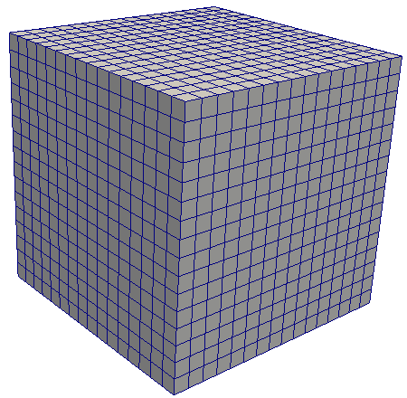
Figure 5: Hexahedral mesh of the matrix domain (left) conforming to the fracture network (right) obtained with $n_{x}=16$.

Table 1: Maximum/mean number of own cells, own cells+nodes+fracture faces and own nodes+fracture faces by process for the hexahedral mesh with $n_{x}=128$ and $N_{p}=64,128$.

$N_{p}$	64	128
own cells	32768/32768	16385/16384
own cells+nodes+fracture faces	68985/67126	34831/33563
own nodes+fracture faces	36217/34358	18447/17179

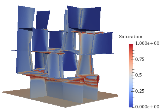
(a) $t=2500$

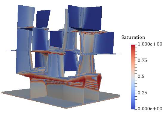
(b) $t=5000$

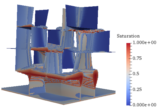
(c) $t=7500$

(d) $t=10000$

Figure 6: Saturation of oil in the fractures and in the matrix domain at different times (in days) for the hexahedral mesh with $n_{x}=128$. A threshold of 0.2 is used for the saturation in the matrix domain.

Table 2 clearly shows that both the total numbers of Newton iterations and of linear solver iterations are almost independent on the number of MPI processes. The Newton solver requires an average of $2.6$ iterations per time step and the GMRES linear solver converges in an average of 40 iterations. These results are very good given the mesh size combined with the large constrast of permeabilities and of space and time scales between the fracture network and the matrix.

Table 2: Number of time steps ($N_{timestep}$), total number of Newton iterations ($N_{newton}$) and total number of linear solver iterations ($N_{gmres}$) vs. number of MPI processes for the two-phase immiscible isothermal flow test case with the hexahedral mesh obtained for $n_{x}=128$.

$N_{p}$	16	32	64	128
$N_{timestep}$	683	683	683	683
$N_{newton}$	1743	1742	1745	1741
$N_{gmres}$	68779	69015	68927	69070
$N_{newton}/N_{timestep}$	2.6	2.6	2.6	2.5
$N_{gmres}/N_{newton}$	39.5	39.6	39.5	39.7

Figure 7 presents the total computation times in hours for different number of MPI processes $N_{p}=16,32,64,128$. The scalability behaves as expected for fully implicit time integration and AMG type preconditioners. It is well known that the AMG preconditioner requires a sufficient number of unknowns per MPI process, say $100000$ as classical order of magnitude, to achieve a linear strong scaling. For this mesh size, leading to roughly $2\times 10^{6}$ unknowns for the pressure block, the scalability is still not far from linear on up to $64$ processes and then degrades more rapidly for $N_{p}=128$. Table 1 shows that the partitioning could be improved by using a weighted graph taking into account the fracture faces. Nevertheless, for this test case, the potential gain seems rather small compared with the loss of parallel efficiency exhibited in Figure 7 which is mainly due to the communication overhead.

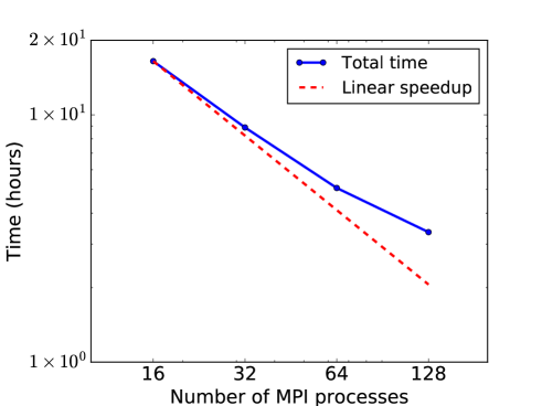
Figure 7: Total computation time vs. number of MPI processes for the two-phase immiscible isothermal flow test case with the hexahedral mesh obtained for $n_{x}=128$.

5.2 Black Oil model

5.2.1 Oil migration

This test case considers a Black Oil model with two components $\mathcal{C}=\{H_{2}O,HC\}$ and two phases $\mathcal{P}=\{\mathrm{water,oil}\}$. The $HC$ component can dissolve in the water phase defined as a mixture of $HC$ and $H_{2}O$ while the oil phase contains only the $HC$ component. The viscosities of the water and oil phases are the same as in the previous test case. The mass densities are defined by

$$\rho^{water}=990\times(1+C_{HC}^{water})\text{ kg/m${}^{3}$},\ \rho^{oil}=700\text{ kg/m${}^{3}$}.$$

The fugacity coefficients $f_{HC}^{\alpha}(P,T,C^{\alpha}),\alpha\in\mathcal{P}$ are defined by

$$\begin{split}&f_{HC}^{water}=1,\\ &f_{HC}^{oil}=\frac{P-P_{2}}{P_{1}-P_{2}}\bar{c}_{1}+\frac{P-P_{1}}{P_{2}-P_{1}}\bar{c}_{2},\end{split}$$

with $P_{1}=1$ MPa, $P_{2}=2$ MPa, and $\bar{c}_{1}=5\times 10^{-3}$, $\bar{c}_{2}=10^{-2}$.

The reservoir is the cubic domain $\Omega=(0,100)^{3}$ in meter and the width of the fractures is fixed to $d_{f}=0.01$ meter. We consider a tetrahedral mesh conforming to the fracture network as exhibited in Figure 8 for a coarse mesh. The mesh used in this subsection contains about $6.2\times 10^{6}$ cells, $9.7\times 10^{5}$ nodes and $7.1\times 10^{4}$ fracture faces. The permeabilities are isotropic and fixed to $\Lambda_{m}=10^{-15}$ m² in the matrix domain and to $\Lambda_{f}=10^{-11}$ m² in the fracture network. The porosities in the matrix domain and in the fractures are $\phi_{m}=0.1$ and $\phi_{f}=0.5$ respectively.

As in the previous test case, the reservoir is initially saturated with pure water and oil is injected at the bottom boundaries of the matrix domain and of the fracture network. The initial pressure is hydrostatic with $P=2$ MPa at the bottom boundaries and $P=1$ MPa at the top boundaries.

The linear and nonlinear solver parameters are fixed to $N_{newton}^{max}=35$, $N_{gmres}^{max}=200$, $\epsilon_{gmres}=10^{-4}$, $\epsilon_{newton}=10^{-5}$, and the time stepping parameters are fixed to $t_{f}=10000$ days, $\Delta t^{(0)}=0.5\text{ days}$, $\Delta t^{(1)}=2\text{ days}$, $\Delta t^{(2)}=50\text{ days}$, $\Delta t^{(3)}=100\text{ days}$, $t^{(1)}=180\text{ days}$, $t^{(2)}=2000\text{ days}$, $k_{f}=3$.

Figure 9 and Figure 10 present the oil saturation and the molar fraction of the $HC$ component in the water phase both in the fractures and in the matrix domain at times $t=2500,5000,7500,10000$ days.

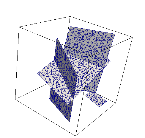
Figure 8: Example of tetrahedral mesh of the matrix domain (left) conforming to the fracture network (right).

Table 3: Maximum/mean number of own cells, own cells+nodes+fracture faces and own nodes+fracture faces by process for the tetrahedral mesh with $6.2\times 10^{6}$ cells and $N_{p}=64,128$.

$N_{p}$	64	128
own cells	96518/96517	48260/48258
own cells+nodes+fracture faces	114898/112762	58063/56381
own nodes+fracture faces	18381/16246	9804/8123

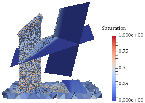
(a) $t=2500$

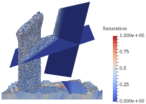
(b) $t=5000$

(c) $t=7500$

(d) $t=10000$

Figure 9: Oil saturation in the fractures and in the matrix domain at different times (in days) for the tetrahedral mesh. A threshold of 0.2 is used for the saturation in the matrix domain.

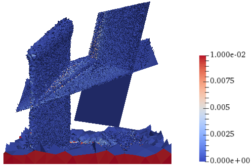
(a) $t=2500$

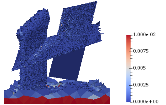
(b) $t=5000$

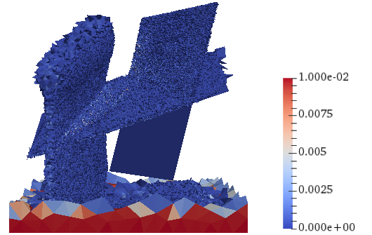
(c) $t=7500$

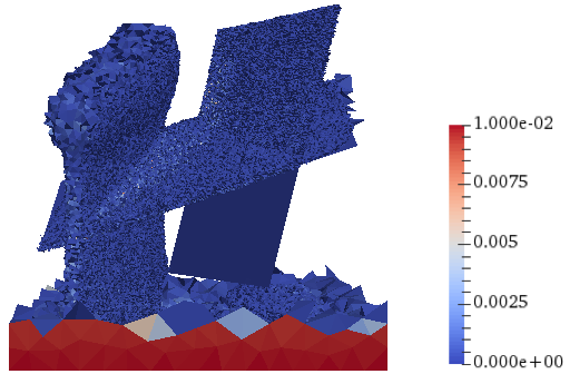
(d) $t=10000$

Figure 10: Molar fraction of the $HC$ component in the water phase in the fractures and in the matrix domain at different times (in days) for the tetrahedral mesh. A threshold of 0.001 is used for the saturation in the matrix domain.

As in the previous test case, table 4 exhibits that both the total numbers of Newton iterations and of linear solver iterations are almost independent on the number of MPI processes. The average number of Newton iteration is $8.8$ per time step. This is a significant increase compared with the previous test case which is due to the phase appearance and disappearance in the Black oil model combined with large contrasts of permeabilities and space and time scales between the matrix and the fractures. On the other hand, the average number of linear solver iterations is roughly $30$ per Newton step which is even better than in the previous test case.

Table 4: Number of time steps ($N_{timestep}$), total number of Newton iterations ($N_{newton}$) and total number of linear solver iterations ($N_{gmres}$) vs. number of MPI processes for the black oil model test case with $6.2\times 10^{6}$ tetrahedral cells.

$N_{p}$	8	16	32	64	128
$N_{timestep}$	249	248	239	246	243
$N_{newton}$	2182	2178	2115	2151	2135
$N_{gmres}$	64340	64567	64649	64039	63277
$N_{newton}/N_{timestep}$	8.8	8.8	8.8	8.7	8.8
$N_{gmres}/N_{newton}$	29.5	29.6	30.6	29.8	29.6

Figure 11 exhibits the total simulation times as a function of the number of MPI processes. The results are similar than in the previous test case. The scalability is very good up to $32$ MPI processes and degrades for $N_{p}=64$ and $128$ as expected for a number of unknowns in the pressure block roughly equal to $10^{6}$. Table 3 shows the maximum and mean number of own d.o.f. by process for $N_{p}=64,128$ with a larger disbalance for own nodes + fracture faces than in the previous test case but still quite smaller than the loss of parallel efficiency exhibited in Figure 11 which is mainly due to the communication overhead.

Figure 11: Total computation time vs. number of MPI processes for the black oil model test case with tetrahedral mesh.

5.2.2 Water injection

We modify the previous test case using the new fracture width $d_{f}=0.001$ meter and injecting pure water instead of oil at the bottom boundary with a bottom pressure of $3$ MPa. The relative permeabilities are modified using a residual water saturation $S_{r}^{w}=0.2$ and the initial water saturation is fixed to $S^{w}=S_{r}^{w}$. The time stepping parameters are fixed to $t_{f}=5000$ days, $\Delta t^{(0)}=0.001\text{ days}$, $\Delta t^{(1)}=30\text{ days}$, $\Delta t^{(2)}=100\text{ days}$, $\Delta t^{(3)}=30\text{ days}$, $t^{(1)}=600\text{ days}$, $t^{(2)}=2000\text{ days}$, $k_{f}=3$.

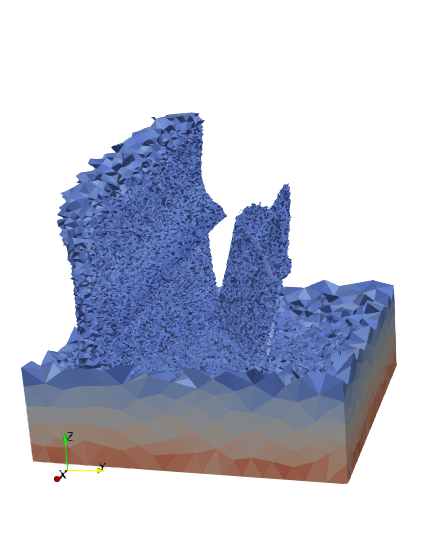
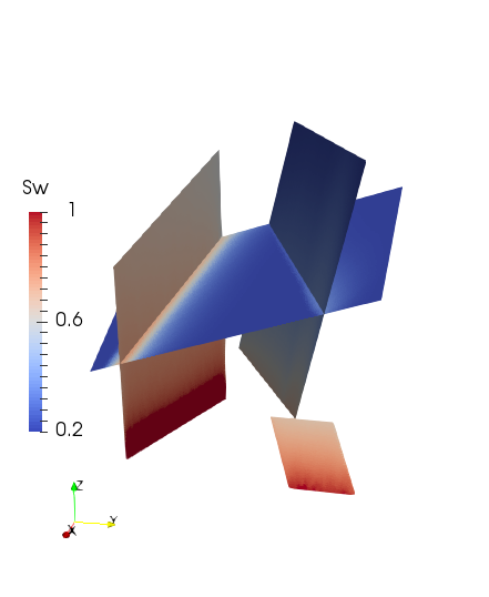
Figure 12: Water saturation at time $t_{f}$ in the matrix (left figure with a threshold of $S^{w}=0.3$) and in the fractures (right) for the Black oil test case with water injection.

Table 5: Number of time steps ($N_{timestep}$), total number of Newton iterations ($N_{newton}$) and total number of linear solver iterations ($N_{gmres}$) vs. number of MPI processes / mesh size for the water injection black oil model test case.

$N_{p}$ / nb of cells	16/$1.17\times 10^{6}$	32/$2.03\times 10^{6}$	64/$4.11\times 10^{6}$
$N_{timestep}$	187	187	190
$N_{newton}$	633	647	688
$N_{gmres}$	8841	10168	12889
CPU time (s)	1213	1424	1940
CPU time / $N_{gmres}$	0.137	0.140	0.151

In order to investigate the weak scalability of the code, Table 5 exhibits the numerical behavior of the simulation obtained for this test case using tetrahedral meshes with $1.17\times 10^{6}$, $2.03\times 10^{6}$, $4.11\times 10^{6}$ cells on respectively $N_{p}=16,32,64$ processes. The number of Newton iterations as well as the total number of GMRES iterations increase only moderately with the mesh size. The CPU time per GMRES iteration exhibits a good weak scalability for $N_{p}=16,32,64$ processes.

5.3 Non-isothermal liquid-gas simulation with a large discrete fault network

We consider in this subsection a single $H_{2}O$ component liquid-gas non-isothermal model with $\mathcal{P}=\{\mathrm{water,gas}\}$ and $\mathcal{C}=\{H_{2}O\}$. The thermodynamical laws providing the phase molar densities, viscosities, internal energies, and enthalpies as well as the saturation vapor pressure are obtained from [43]. The thermal conductivity is fixed to $\lambda=2$ W m^-1 K^-1 and the rock volumetric internal energy is defined by $E_{r}(T)=c_{p}^{r}T$ with $c_{p}^{r}=16.10^{5}$ J m^-3 K^-1. The gravity is not considered in this test case which means that the solution is 2 dimensional.

The fault network is provided by M. Karimi-Fard and A. Lapène from Stanford University and TOTAL as well as the prismatic mesh of the domain $\Omega=(0,5888)\times(0,3157)\times(0,200)$ (meters) which contains about $1.3\times 10^{6}$ prismatic cells, $3.4\times 10^{6}$ nodes and $7.1\times 10^{5}$ fault faces. The 3D mesh is defined by the tensor product of a triangular 2D mesh with a uniform vertical 1D mesh with $10$ intervals. The fault network contains $581$ connected components. The fault width is set to $d_{f}=1$ m and the permeabilities are isotropic and fixed to $\Lambda_{m}=10^{-15}$ m² in the matrix domain and to $\Lambda_{f}=10^{-12}$ m² in the fault network. The porosities in the matrix domain and in the faults are $\phi_{m}=0.1$ and $\phi_{f}=0.1$ respectively.

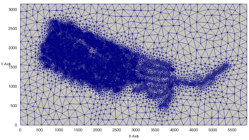
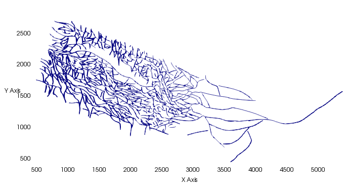
Figure 13: Horizontal view of the prismatic mesh of the matrix domain coarsened by a factor $2$ in the $x,y$ directions (left) conforming to the fault network (right).

Table 6: Maximum/mean number of own cells, own cells+nodes+fracture faces and own nodes+fracture faces by process for the prismatic mesh with $1.3\times 10^{6}$ cells and $N_{p}=64,128$.

$N_{p}$	64	128
own cells	20214/20212	10107/10106
own cells+nodes+fracture faces	33767/33016	17010/16508
own nodes+fracture faces	13554/12803	6903/6401

Let us set $\Gamma_{output}=\{(x,y,z)\in\Omega\ |\ x=0\}$ and $\Gamma_{input}=\{(x,y,z)\in\Omega\ |\ x=5888\}$. The simulation domain is initially in liquid phase with $P=1$ MPa and $T=450$ K. Dirichlet boundary conditions are imposed at $\Gamma_{output}$ with $P=1$ MPa and $T=450$ K (liquid phase) and at $\Gamma_{input}$ with $P=2$ MPa and $T=550$ K (gas phase). The remaining boundaries are considered impervious to mass and energy.

The linear and nonlinear solver parameters are fixed to $N_{newton}^{max}=50$, $N_{gmres}^{max}=300$, $\epsilon_{gmres}=10^{-4}$, $\epsilon_{newton}=10^{-6}$, and the time stepping parameters are fixed to $t_{f}=280000$ days, $\Delta t^{(0)}=1000\text{ days}$, $\Delta t^{(1)}=10000\text{ days}$, $k_{f}=1$.

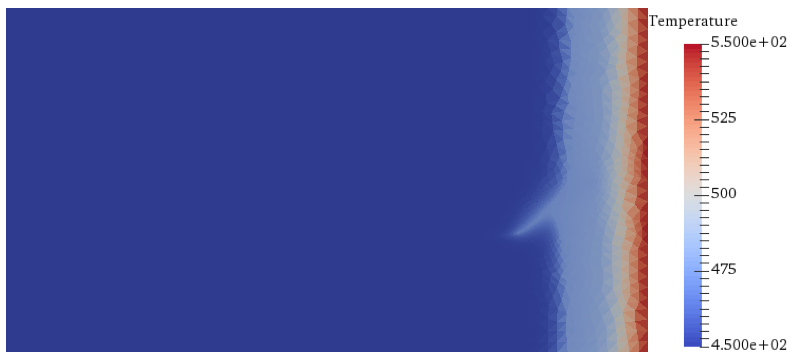
(a) $t=70000$

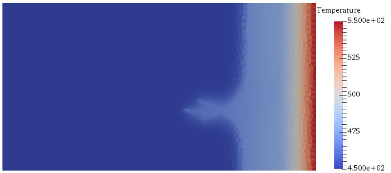
(b) $t=140000$

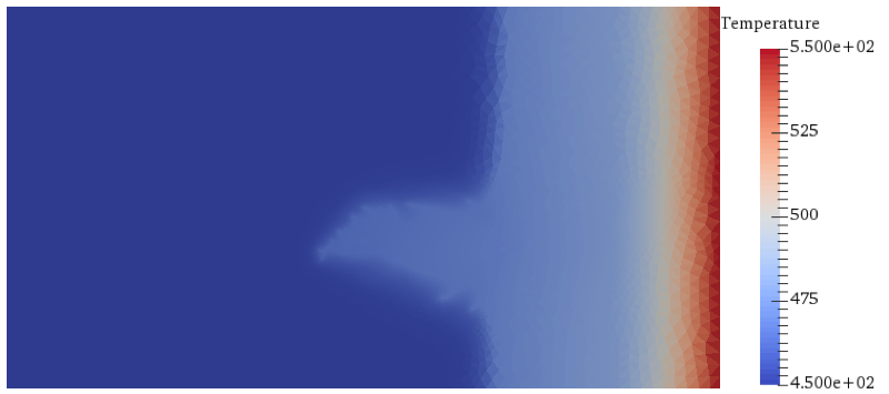
(c) $t=210000$

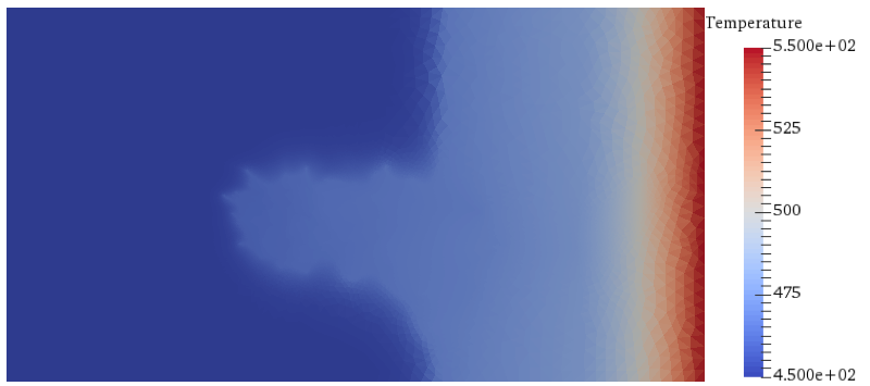
(d) $t=280000$

Figure 14: Temperature in the matrix domain for the non-isothermal test case on the prismatic mesh.

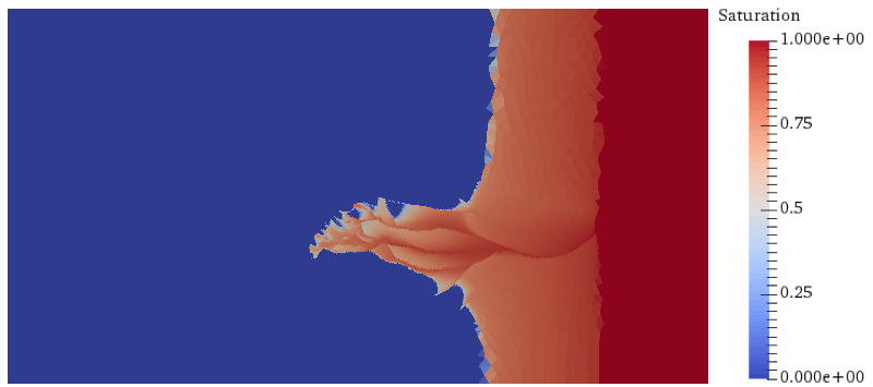
(a) $t=70000$

(b) $t=140000$

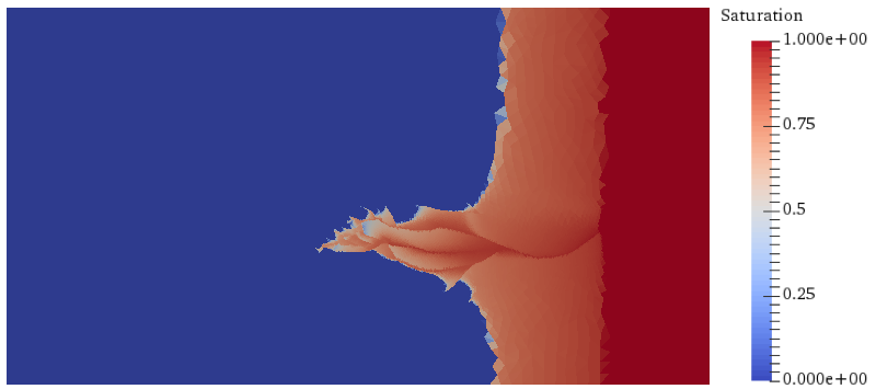
(c) $t=210000$

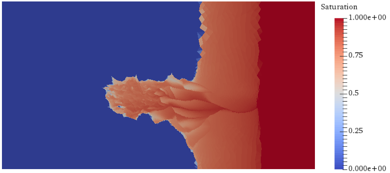
(d) $t=280000$

Figure 15: Gas saturation in the matrix domain for the non-isothermal test case on the prismatic mesh.

Figures 14 and 15 exhibit the temperature and the gas saturation at different times. Table 7 shows the total number of Newton iterations and the total number of linear solver iterations which are, as for the previous test cases, almost independent on the number of MPI processes $N_{p}=32,64,128,256$. The average number of Newton iterations per time step is $20$. This is a high value but typical for such non-isothermal flows combining high non linearities in the thermodynamical laws and highly contrasted matrix and fault properties and scales. On the other hand, the number of linear solver iterations, roughly $60$ per Newton step, remains very good. Simarly as in the previous test cases, the scalability of the total simulation time with respect to the number of MPI processes presented in Figure 16 is very good from $32$ to $64$ processes and then degrades for $N_{p}=128$ and $256$ due to a too small number of unknowns in the pressure block per MPI process. Table 6 shows the maximum and mean number of own d.o.f. by process for $N_{p}=64,128$ with similar conclusions as in the previous test cases.

Table 7: Number of time steps ($N_{timestep}$), total number of Newton iterations ($N_{newton}$) and total number of linear solver iterations ($N_{gmres}$) vs. number of MPI processes for the non-isothermal test case on the prismatic mesh.

$N_{p}$	32	64	128	256
$N_{timestep}$	300	318	303	289
$N_{newton}$	5890	6012	5946	5885
$N_{gmres}$	372671	370954	383523	391250
$N_{newton}/N_{timestep}$	19.6	18.9	19.6	20.4
$N_{gmres}/N_{newton}$	63.3	61.7	64.5	66.5

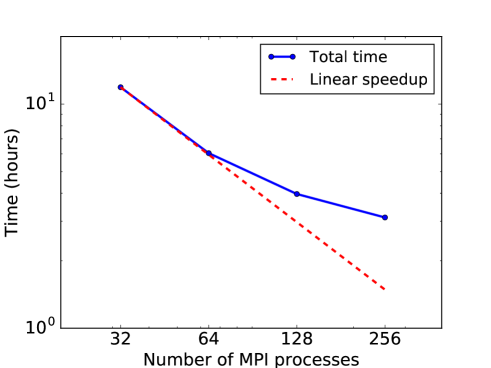
Figure 16: Total computation time vs. number of MPI processes for the non-isothermal test case on the prismatic mesh.

5.4 Thermal convection test case with Cartesian mesh

This test case considers the same physical two-phase non-isothermal model as in the previous subsection but including gravity. The simulation domain is $\Omega=(0,3000)^{3}$ in meters. The mesh is a 3D uniform Cartesian mesh which contains $240^{3}$ cells. The fault network is defined by

$$\Gamma=\{(x,y,z)\in\Omega\ |\ x=1500\ \mathrm{or}\ y=1500\ \mathrm{and}\ 500\leqslant z\leqslant 2500\},$$

with fault width fixed to $d_{f}=1$ meter. The permeabilities are isotropic and set to $\Lambda_{m}=10^{-15}$ m² in the matrix domain and to $\Lambda_{f}=10^{-12}$ m² in the fault network. The porosities in the matrix domain and in the faults are $\phi_{m}=0.1$ and $\phi_{f}=0.5$ respectively.

The domain is initially in liquid phase with a fixed temperature $293$ K and an hydrostatic pressure defined by its value $P=1$ bar at the top boundary. The temperature is fixed to $623$ K (liquid phase) at the bottom boundary which is impervious to mass. At the top boundary, the pressure is set to $1$ bar and the temperature to $293$ K (liquid phase). A zero flux for both mass and temperature is imposed at the lateral boundaries of the domain.

The linear and nonlinear solver parameters are fixed to $N_{newton}^{max}=25$, $N_{gmres}^{max}=300$, $\epsilon_{gmres}=10^{-4}$, $\epsilon_{newton}=10^{-5}$, and the time stepping parameters are fixed to $t_{f}=2\times 10^{7}$ days, $\Delta t^{(0)}=5\times 10^{5}\text{ days}$, $\Delta t^{(1)}=5\times 10^{5}\text{ days}$, $\Delta t^{(2)}=10^{5}\text{ days}$, $\Delta t^{(3)}=5\times 10^{3}\text{ days}$, $t^{(1)}=2.5\times 10^{6}\text{ days}$, $t^{(2)}=1.7\times 10^{7}\text{ days}$, $k_{f}=3$.

Figure 17 shows the temperature in the faults and in the matrix domain at times $t=1\times 10^{7}$ days and $t=t_{f}$. In addition, we present in Figure 18 the gas saturation at final time.

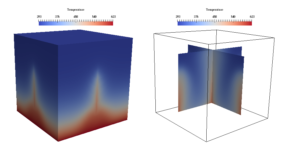
(a) $t=1\times 10^{7}$ days

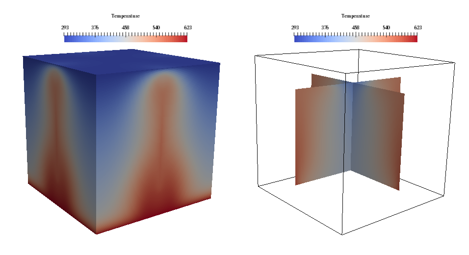
(b) $t=2\times 10^{7}$ days

Figure 17: Temperature in the faults and in the matrix domain at different times (days).

Figure 18: Saturation of gas in the matrix domain at the final time $t_{f}=2\times 10^{7}$ days.

In this test case, the thermal convection leads to convective instabilities which are triggered by the numerical round-off errors. Hence it is not appropriate to make scalability tests since the solution will depend on the number of MPI processes. Therefore, we only exhibit in Table 8 the results obtained for $N_{p}=256$. This simulation lasts $40.57$ hours. The convective instabilities and strong nonlinearities require a small time step in order to obtain Newton’s convergence, especially at the end of the simulation when the gas phase appears.

Table 8: Number of time steps ($N_{timestep}$), total number of Newton iterations ($N_{newton}$) and total number of linear solver iterations ($N_{gmres}$) for the thermal convection test case on the Cartesian mesh where $N_{p}=256$.

$N_{timestep}$	3117
$N_{newton}$	6712
$N_{gmres}$	238600
$N_{newton}/N_{timestep}$	2.2
$N_{gmres}/N_{newton}$	35.5

5.5 Thermal convection test case with tetrahedral mesh

This last test case considers the same physical two-phase non-isothermal model as in the previous subsection, but with the tetrahedral mesh shown in Figure 8 and rescaled to a larger domain $\Omega=(0,3000)^{3}$ in meters. The fault width is fixed to $d_{f}=1$ meter. The permeabilities are isotropic and set to $\Lambda_{m}=10^{-14}$ m² in the matrix domain and to $\Lambda_{f}=10^{-12}$ m² in the fault network. The porosity in the matrix domain is set to $\phi_{m}=0.25$, and to $\phi_{f}=0.35$ in the fault network.

At the intersection $\{z=0\}\cap\Gamma$ of the bottom boundary with the fault network, the temperature is fixed to $623$ K and a mass flow rate of $100$ kg/s is uniformly prescribed. At the matrix bottom boundary, the temperature is set as $473$ K and the mass flow rate is set to zero. At the top boundary, the pressure is set to $10^{5}$ Pa and the temperature to $293$ K (liquid phase). A zero flux for both mass and temperature is imposed at the lateral boundaries of the domain. The simulation domain is initially in liquid phase with an hydrostatic pressure defined by the pressure boundary condition at the top boundary and with a linear temperature between $293$K at the top boundary and $473$K at the bottom boundary.

We set the linear and nonlinear solver parameters to $N_{newton}^{max}=30$, $N_{gmres}^{max}=150$, $\epsilon_{gmres}=10^{-5}$, $\epsilon_{newton}=10^{-6}$, and the time stepping parameters are fixed to $t_{f}=2\times 10^{5}$ days, $\Delta t^{(0)}=50\text{ days}$, $\Delta t^{(1)}=1000\text{ days}$, $\Delta t^{(2)}=50\text{ days}$, $t^{(1)}=5.8\times 10^{4}\text{ days}$, $k_{f}=2$.

Figure 19 exhibits the temperature in the faults (left) and the gas saturation in the faults and in the matrix domain (right) at times $t=7\times 10^{4}$ days and $t=t_{f}$.

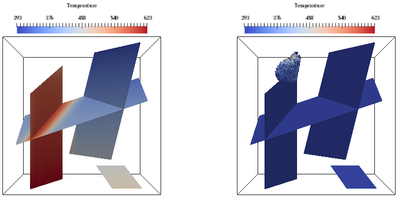
(a) $t=7\times 10^{4}$ days

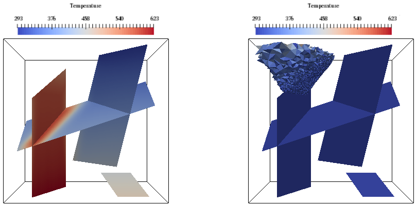
(b) $t=2\times 10^{5}$ days

Figure 19: Left: temperature in the faults at different times (days). Right: saturation of gas in the faults and in the matrix domain at different times (days) where a threshold of 0.0001 is used on the matrix domain.

Table 9 shows the total number of Newton iterations and the total number of linear solver iterations. We present the total computation time in hours for different number of MPI processes $N_{p}=16,32,64,128$ in Figure 20. The scalability is similar to the one obtained with the black oil model test case using the same tetrahedral mesh as shown in Figure 11.

Table 9: Number of time steps ($N_{timestep}$), total number of Newton iterations ($N_{newton}$) and total number of linear solver iterations ($N_{gmres}$) vs. number of MPI processes for the thermal convection test case with tetrahedral mesh.

$N_{p}$	16	32	64	128
$N_{timestep}$	2939	2946	2950	2946
$N_{newton}$	10043	10259	10352	10074
$N_{gmres}$	151993	155925	158124	153836
$N_{newton}/N_{timestep}$	3.4	3.5	3.5	3.4
$N_{solver}/N_{newton}$	15.1	15.2	15.3	15.3

Figure 20: Total computation time vs. number of MPI processes for the thermal convection test with tetrahedral mesh.

6 Conclusion

In this paper, a discrete fracture model accounting for non-isothermal compositional multiphase Darcy flows was introduced. The geometry takes into account complex networks of intersecting, immersed or non immersed planar fractures. The physical model accounts for an arbitrary nonzero number of components in each phase allowing to model immiscible, partially miscible or fully miscible flows. The discretization is based on the VAG finite volume scheme adapted to unstructured polyhedral meshes and to anisotropic heterogeneous media. The time integration is fully implicit in order to avoid strong restrictions on the time step due to the high velocities and small volumes in the fractures. The discrete model is implemented in parallel based on the SPMD paradigm and using one layer of ghost cells in order to assemble the systems locally on each processor. The CPR-AMG preconditioner was investigated to deal with non-isothermal models.

The numerical results exhibit the ability of our discrete model to combine complex physics including non-isothermal flows, thermodynamical equilibrium and buoyancy forces with fracture networks including highly contrasted matrix fracture permeabilities. The parallel scalability requires, as expected for fully implicit discretizations when using AMG type preconditioners, that the number of degrees of freedom per processor is kept high enough.

References

- [1] C. Alboin, J. Jaffré, J. Roberts, C. Serres, Modeling fractures as interfaces for flow and transport in porous media, Vol. 295, 2002, pp. 13–24.
- [2] E. Flauraud, F. Nataf, I. Faille, R. Masson, Domain decomposition for an asymptotic geological fault modeling, Comptes Rendus Mécanique 331 (12) (2003) 849–855.
- [3] I. I. Bogdanov, V. V. Mourzenko, J.-F. Thovert, P. M. Adler, Two-phase flow through fractured porous media, Physical Review E 68 (2).
- [4] M. Karimi-Fard, L. Durlofsky, K. Aziz, An efficient discrete-fracture model applicable for general-purpose reservoir simulators, SPE Journal 9 (02) (2004) 227–236.
- [5] V. Martin, J. Jaffré, J. E. Roberts, Modeling fractures and barriers as interfaces for flow in porous media, SIAM Journal on Scientific Computing 26 (5) (2005) 1667–1691.
- [6] K. Brenner, M. Groza, C. Guichard, G. Lebeau, R. Masson, Gradient discretization of hybrid-dimensional Darcy flows in fractured porous media, Numerische Mathematik 134 (3) (2016) 569–609.
- [7] P. Angot, F. Boyer, F. Hubert, Asymptotic and numerical modelling of flows in fractured porous media, ESAIM: Mathematical Modelling and Numerical Analysis 43 (2) (2009) 239–275.
- [8] K. Brenner, J. Hennicker, R. Masson, P. Samier, Gradient discretization of hybrid-dimensional Darcy flow in fractured porous media with discontinuous pressures at matrix-fracture interfaces, IMA Journal of Numerical Analysis.
- [9] F. Xing, R. Masson, S. Lopez, Parallel Vertex Approximate Gradient discretization of hybrid-dimensional Darcy flow and transport in discrete fracture networks, Computational Geosciences.
- [10] V. Reichenberger, H. Jakobs, P. Bastian, R. Helmig, A mixed-dimensional finite volume method for two-phase flow in fractured porous media, Advances in Water Resources 29 (7) (2006) 1020–1036.
- [11] H. Hoteit, A. Firoozabadi, An efficient numerical model for incompressible two-phase flow in fractured media, Advances in Water Resources 31 (6) (2008) 891–905.
- [12] J. Jaffré, M. Mnejja, J. Roberts, A discrete fracture model for two-phase flow with matrix-fracture interaction, Procedia Computer Science 4 (2011) 967–973.
- [13] K. Brenner, M. Groza, C. Guichard, R. Masson, Vertex Approximate Gradient scheme for hybrid-dimensional two-phase Darcy flows in fractured porous media, ESAIM: Mathematical Modelling and Numerical Analysis 2 (49) (2015) 303–330.
- [14] K. Brenner, J. Hennicker, R. Masson, P. Samier, Hybrid-dimensional modelling and discretization of two phase darcy flow through DFN in porous media, in: ECMOR XV- 15th European Conference on the Mathematics of Oil Recovery, 2016.
- [15] H. Haegland, A. Assteerawatt, H. Dahle, G. Eigestad, R. Helmig, Comparison of cell- and vertex-centered discretization methods for flow in a two-dimensional discrete-fracture-matrix system, Advances in Water resources 32 (2009) 1740–1755.
- [16] X. Tunc, I. Faille, T. Gallouët, M. C. Cacas, P. Havé, A model for conductive faults with non-matching grids, Computational Geosciences 16 (2) (2012) 277–296.
- [17] T. Sandve, I. Berre, J. Nordbotten, An efficient multi-point flux approximation method for Discrete Fracture-Matrix simulations, Journal of Computational Physics 231 (9) (2012) 3784–3800.
- [18] R. Ahmed, M. Edwards, S. Lamine, B. Huisman, M. Pal, Control-volume distributed multi-point flux approximation coupled with a lower-dimensional fracture model, Journal of Computational Physics 284 (2015) 462–489.
- [19] R. Ahmed, M. G. Edwards, S. Lamine, B. A. Huisman, M. Pal, Three-dimensional control-volume distributed multi-point flux approximation coupled with a lower-dimensional surface fracture model, Journal of Computational Physics 303 (2015) 470–497.
- [20] J. Droniou, R. Eymard, T. Gallouët, R. Herbin, Gradient schemes: a generic framework for the discretisation of linear, nonlinear and nonlocal elliptic and parabolic equations, Math. Models Methods Appl. Sci. 13 (23) (2013) 2395–2432.
- [21] I. Faille, A. Fumagalli, J. Jaffré, J. E. Roberts, Model reduction and discretization using hybrid finite volumes of flow in porous media containing faults, Computational Geosciences 20 (2016) 317–339.
- [22] P. F. Antonietti, L. Formaggia, A. Scotti, M. Verani, N. Verzott, Mimetic finite difference approximation of flows in fractured porous media, ESAIM M2AN 50 (2016) 809–832.
-
[23]
J. Droniou, R. Eymard, T. Gallouët, C. Guichard, R. Herbin,
The Gradient
discretization method: A framework for the discretization of linear and
nonlinear elliptic and parabolic problems, Tech. rep. (2016).
URL https://hal.archives-ouvertes.fr/hal-01382358 - [24] J. E. Monteagudo, A. Firoozabadi, Control-volume model for simulation of water injection in fractured media: incorporating matrix heterogeneity and reservoir wettability effects, SPE Journal 12 (03) (2007) 355–366.
- [25] R. Eymard, C. Guichard, R. Herbin, R. Masson, Vertex-centred discretization of multiphase compositional Darcy flows on general meshes, Computational Geosciences 16 (4) (2012) 987–1005.
- [26] S. K. Matthai, A. A. Mezentsev, M. Belayneh, Finite element - node-centered finite-volume two-phase-flow experiments with fractured rock represented by unstructured hybrid-element meshes, SPE Reservoir Evaluation & Engineering 10 (06) (2007) 740–756.
- [27] C. D’Angelo, A. Scotti, A mixed finite element method for Darcy flow in fractured porous media with non-matching grids, ESAIM: Mathematical Modelling and Numerical Analysis 46 (2) (2012) 465–489.
- [28] A. Fumagalli, A. Scotti, A. Cangiani, R. L. Davidchack, E. Georgoulis, A. N. Gorban, A reduced model for flow and transport in fractured porous media with non-matching grids, Numerical Mathematics and Advanced Applications (2013) 499–507.
- [29] S. Berrone, S. Pieraccini, S. Scialò, An optimization approach for large scale simulations of discrete fracture network flows, Journal of Computational Physics 256 (2014) 838–853.
- [30] N. Schwenck, B. Flemisch, R. Helmig, B. Wohlmuth, Dimensionally reduced flow models in fractured porous media: crossings and boundaries, Computational Geosciences 19 (2015) 1219–1230.
- [31] K. Brenner, M. Groza, L. Jeannin, R. Masson, J. Pellerin, Immiscible two-phase Darcy flow model accouting for vanishing and discontinuous capillary pressures: application to the flow in fracture porous media, in: ECMOR XV- 15th European Conference on the Mathematics of Oil Recovery, 2016.
- [32] K. Brenner, J. Hennicker, R. Masson, P. Samier, Hybrid-dimensional modelling of two-phase flow through fractured porous media with enhanced matrix fracture transmission conditions, Tech. rep. (2017).
- [33] K. Coats, Implicit compositional simulation of single-porosity and dual-porosity reservoirs, in: SPE Symposium on Reservoir Simulation, Society of Petroleum Engineers, 1989.
- [34] H. Class, R. Helmig, P. Bastian, Numerical simulation of non-isothermal multiphase multicomponent processes in porous media.: 1. An efficient solution technique, Advances in Water Resources 25 (2002) 533–550.
- [35] S. Lacroix, Y. V. Vassilevski, M. F. Wheeler, Decoupling preconditioners in the implicit parallel accurate reservoir simulator (IPARS), Numerical Linear Algebra with Applications 8 (8) (2001) 537–549.
- [36] R. Scheichl, R. Masson, J. Wendebourg, Decoupling and block preconditioning for sedimentary basin simulations, Computational Geosciences 7 (4) (2003) 295–318.
- [37] K. Aziz, A. Settari, Petroleum Reservoir Simulation, Applied Science Publishers, 1979.
- [38] R. Eymard, C. Guichard, R. Herbin, Small-stencil 3D schemes for diffusive flows in porous media, ESAIM: Mathematical Modelling and Numerical Analysis 46 (2) (2012) 265–290.
- [39] V. E. Henson, U. M. Yang, BoomerAMG: A parallel algebraic multigrid solver and preconditioner, Applied Numerical Mathematics 41 (1) (2002) 155–177.
- [40] Y. Achdou, P. Bonneau, R. Masson, P. Quandalle, Block preconditioning and multigrid solvers for linear systems in reservoir simulations, in: European Conference on Mathematics of Oil Recovery ECMOR X, 2006.
- [41] G. Karypis, V. Kumar, A Fast and high quality multilevel scheme for partitioning irregular graphs, SIAM Journal on Scientific Computing 20 (1) (1998) 359–392.
- [42] S. Balay, M. Adams, J. Brown, P. Brune, K. Buschelman, V. Eijkhout, H. Zhang, PETSc Users Manual. Revision 3.5, Tech. rep. (2015).
- [43] E. Schmidt, Properties of water and steam in S.I. units, Springer-Verlag, 1969.