Heidi Seibold, Torsten Hothorn, Achim Zeileis Heidi Seibold, Torsten Hothorn
Department of Biostatistics
Epidemiology, Biostatistics and Prevention Institute
University of Zurich
Hirschengraben 84
CH-8001 Zurich, Switzerland
Heidi Seibold
Institute for Medical Information Processing, Biometry, and Epidemiology
Ludwig-Maximilans-Universität München
Marchioninistr. 15
81377 Munich
Achim Zeileis
Department of Statistics
Faculty of Economics and Statistics
Universität Innsbruck
Universitätsstr. 15
A-6020 Innsbruck, Austria
Model-based trees are used to find subgroups in data which differ with respect to model parameters. In some applications it is natural to keep some parameters fixed globally for all observations while asking if and how other parameters vary across subgroups. Existing implementations of model-based trees can only deal with the scenario where all parameters depend on the subgroups. We propose partially additive linear model trees (PALM trees) as an extension of (generalised) linear model trees (LM and GLM trees, respectively), in which the model parameters are specified a priori to be estimated either globally from all observations or locally from the observations within the subgroups determined by the tree. Simulations show that the method has high power for detecting subgroups in the presence of global effects and reliably recovers the true parameters. Furthermore, treatment-subgroup differences are detected in an empirical application of the method to data from a mathematics exam: the PALM tree is able to detect a small subgroup of students that had a disadvantage in an exam with two versions while adjusting for overall ability effects. subgroup analysis, model-based recursive partitioning, GLM, tree

Generalised Linear Model Trees with Global Additive Effects

1 Introduction

Model-based recursive partitioning (Zeileis et al, 2008) is used to partition data into groups that differ in terms of the parameters in the model. The method can be applied, for example, to find subgroups in a clinical trial which differ in terms of treatment effect on a health score (e.g. Seibold et al, 2016) or areas in a city which differ in terms of the influence of square metres on the rent price. Sometimes there are parameters in the model that one wants to fix for all groups, e.g. the effect of smoking on the health outcome in the clinical trial or the effect of inflation/deflation on rent prices. This, however, is not possible in model-based recursive partitioning as described in Zeileis et al (2008). Here we propose an algorithm called PALM tree that is similar to model-based recursive partitioning but allows fixing parameters over all groups, i.e. only some parameters depend on the tree structure.

There have been several developments in the past years toward the direction of combining models and trees, where one part of the model follows a tree structure and one part does not. The Simultaneous Threshold Interaction Modeling Algorithm (STIMA, Dusseldorp et al, 2010) starts off with a main effects model and adds interactions based on a tree. Fokkema et al (2017) proposed GLMM tree, a method that is similar to PALM tree, but is used to fix random effects in a generalised linear mixed-effects model (GLMM) instead of – as in PALM tree – further fixed effects. Other approaches going in the direction of GLMM tree are RE-EM tree (Sela and Simonoff, 2012) and MERT (Hajjem et al, 2011).

In the literature on subgroup analyses for the estimation of treatment effects, special tree-based procedures have been proposed (see, e.g. Doove et al, 2014). These methods are commonly used in the analysis of clinical trials, but are equally relevant in contexts such as marketing studies evaluating different marketing strategies or studies on website user behaviour, where users are randomly served one of two website versions (A/B testing). Sies and Van Mechelen (2017) review some of the methods in a setting where there are some model covariates with fixed parameters across all subgroups and varying treamtent effect. One promising method in this review is a method by Zhang et al (2012) which estimates rules of optimal treatment for each patient subgroup (optimal treatment regimes).

The following sections unfold as follows: In Section 2 we will first describe GLMs and GLM trees as the basics needed for PALM trees and then go into how PALM trees are computed. Furthermore we will show how model-based trees (LM trees, GLM trees and PALM trees) can be used for finding subgroups with differential treatment effects. In Section 3 we will show the results of a simulation study in which we compare LM tree, PALM tree, STIMA and the optimal treatment regime method by Zhang et al (2012). In Section 4 we will apply the PALM tree to data of a mathematics exam, where the endpoint is performance in the exam, the “treatment” is the student group (early morning or late group) and the known prognostic factor is the performance in online tests the students participate in during the semester. Finally we will discuss strengths and limitations of model-based trees in general and PALM trees in particular.

2 Methods

In this section we first describe the basics needed for PALM trees – GLMs and GLM trees – and then introduce PALM trees and how GLMs and GLM trees are used in the PALM tree algorithm. We focus on GLMs since LMs are a special case of GLMs.

2.1 Basics: GLMs and GLM trees

2.1.1 GLMs

GLMs model the expected response $\mu=\mathbb{E}({y})$ given the covariates $\mathbf{x}$. To fix notation we write the GLM as $g({\mu})=\mathbf{x}^{\top}\boldsymbol{\beta}$ where $g$ denotes the link function and $\mathbf{x}^{\top}\boldsymbol{\beta}$ the linear predictor with coefficient vector $\boldsymbol{\beta}$. The coefficients are estimated by maximising the log-likelihood. The observation-wise log-likelihood contributions are denoted by $l((y,\mathbf{x})_{i},\boldsymbol{\beta})$ with $i=1,\dots,n$ indexing the $i$-th observation and $l$ is defined depending on the appropriate exponential family chosen for the GLM (Gaussian, Poisson, etc.).

In the following we will make use of two refinements commonly used in GLMs: (a) interactions and (b) offsets. Interactions are effects combinding two or more covariates and can be employed to establish subgroup-specific coefficient vectors in a single model:

$$g({\mu})=\mathbf{\tilde{x}}^{\top}\boldsymbol{\tilde{\beta}}=I(\text{subgroup}_{1})\cdot\mathbf{x}^{\top}\boldsymbol{\beta}_{1}~{}+I(\text{subgroup}_{2})\cdot\mathbf{x}^{\top}\boldsymbol{\beta}_{2}~{}+\dots$$ (1)

where $I(\text{subgroup}_{j})$ equals $1$ for observations in the $j$-th subgroup and $0$ for others. The combined coefficient vector is simply $\boldsymbol{\tilde{\beta}}=\boldsymbol{\beta}_{1}^{\top},\boldsymbol{\beta}_{2}^{\top},\dots)^{\top}$

Offsets in GLMs are useful for incorporating additional terms whose effects are known or fixed into the linear predictor :

$$g({\mu})=\mathbf{x}^{\top}\boldsymbol{\beta}+\text{offset}.$$ (2)

Thus, the offset behaves like an additional regressor whose coefficient is not estimated but fixed, e.g. to $1$. A prominent example for offsets in GLMs is the modeling of rates in Poisson regression, where $\text{offset}=1\cdot\log(\text{exposure})$.

2.1.2 GLM trees

Tree algorithms generally split the data recursively into disjoint subgroups (also called nodes) starting from the so-called root node containing all data and employing certain split points in the so-called split variables. In case of GLM trees, the idea is to (1) estimate the parameters in a GLM using the current sample (starting with the full data set), (2) assess whether the parameters are stable over the split variables considered, (3) split the sample along the variable associated with the highest parameter instability, (4) repeat the previous steps recursively until some stopping criterion is met (e.g., with respect to the size of the sample or the instability of the parameters). Various algorithms have been suggested that can be employed for such GLM-based recursive partitioning, including GUIDE (Loh, 2002), CTree (Hothorn et al, 2006), or MOB (Zeileis et al, 2008) where the latter is used subsequently and explained in more detail in Section 2.2.1.

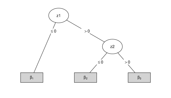
Figure 1: Example of a model-based tree.

Figure 1 shows an example tree structure that could be found by a GLM tree with

$$\boldsymbol{\beta}(\mathbf{z}) =\begin{cases}\boldsymbol{\beta}_{1}&\quad\text{if }~{}z_{1}\leq 0\\ \boldsymbol{\beta}_{2}&\quad\text{if }~{}(z_{1}>0)~{}\wedge~{}(z_{2}\leq 0)\\ \boldsymbol{\beta}_{3}&\quad\text{if }~{}(z_{1}>0)~{}\wedge~{}(z_{2}>0).\end{cases}$$ (3)

The parameters $\boldsymbol{\beta}_{1}$, $\boldsymbol{\beta}_{2}$, and $\boldsymbol{\beta}_{3}$ can be estimated by three separate models for the three subgroups or by using interaction terms as in Equation 1 ($I(\text{subgroup}_{1})=I(z_{1}\leq 0)$ etc.). To make the role of the split variables more explicit we from now on write $\mathbf{x}^{\top}\boldsymbol{\beta}(\mathbf{z})$ instead of $\mathbf{\tilde{x}}^{\top}\boldsymbol{\tilde{\beta}}$. $\boldsymbol{\beta}(\mathbf{z})$ is the interaction effect between covariates $\mathbf{x}$ and the subgroups defined by the split variables $\mathbf{z}$.

2.2 Extension: PALM trees

GLM trees assume that all parameters are subgroup specific. This does not necessarily have to be the case. PALM trees address this issue and offer a compromise between GLM trees and GLMs by having one part in which the parameters depend on subgroups (these are again denoted by $\boldsymbol{\beta}(\mathbf{z})$) and another part in which the parameters are the same for all subjects/subgroups (denoted by $\boldsymbol{\gamma}$).

Going from GLMs via GLM trees to PALM trees can be viewed as an evolutionary process where one method evolves from the other. The goal of all three is to appropriately estimate the effect of covariates $\mathbf{x}$ on an outcome ${y}$. The main difference between the three methods is the structure of the linear predictor. While the effects $\boldsymbol{\beta}$ are linear in a GLM, the effects $\boldsymbol{\beta}(\mathbf{z})$ are linear and constant within each subgroup but vary between subgroups, i.e. are subgroup-wise linear. A PALM tree contains globally fixed linear effects $\boldsymbol{\gamma}$ for some covariates $\mathbf{x}_{F}$ and subgroup-wise varying linear effects $\boldsymbol{\beta}(\mathbf{z})$ for other covariates $\mathbf{x}_{V}$. Mathematically this can be expressed as follows:

GLM $$g({\mu})=\mathbf{x}^{\top}\boldsymbol{\beta}$$ (4)

GLM tree $$g({\mu})=\mathbf{x}^{\top}\boldsymbol{\beta}(\mathbf{z})$$ (5)

PALM tree $$g({\mu})=\mathbf{x}_{V}^{\top}\boldsymbol{\beta}(\mathbf{z})+\mathbf{x}_{F}^{\top}\boldsymbol{\gamma}.$$ (6)

In PALM trees the variables $\mathbf{x}_{F}$ with a global effect $\boldsymbol{\gamma}$ have to be defined a priori. Usually $\mathbf{x}_{V}$ and $\mathbf{x}_{F}$ and $\mathbf{z}$ do not overlap although this is, in principle, possible. Note that if the subgroup structure were known, models 5 and 6 could both be estimated as GLMs. Only the fact that it is unknown and has to be detected makes GLM trees and PALM trees necessary. Also, if the global parameter vector $\boldsymbol{\gamma}$ were known, model 6 could be estimated as GLM tree with $\mathbf{x}_{F}^{\top}\boldsymbol{\gamma}$ as offset (as in equation 2). These connections between the methods are leveraged in the PALM tree algorithm.

2.2.1 Algorithm

We now describe the detailed GLM tree and PALM tree algorithms, starting with GLM trees as the PALM tree algorithm uses GLM trees in the estimation process. The GLM tree algorithm is not new and has been explained in depth by Zeileis et al (2008). The following description of the algorithm focuses on the parts that are necessary in order to demonstrate the full concept of the PALM tree algorithm. Note that to notationally distinguish the parameters in the subgroups (e.g. parameter vector in first subgroup $\boldsymbol{\beta}_{1}$) from parameters in the models (e.g. first model parameter $\beta_{(1)}$) we use parentheses. GLM trees are grown as follows, starting with the root node containing all observations:

1. Compute model (4), or equivalently model (5) with a single subgroup ($\boldsymbol{\beta}(\mathbf{z})=\boldsymbol{\beta}$), in the given node.

2. Test for instability in the model parameters with respect to each of the possible subgroup defining variables ${Z}_{1},\dots,{Z}_{J}$:

   • Compute the score contributions

     $$s_{(k)}\left((y,\mathbf{x})_{i},\hat{\boldsymbol{\beta}}\right)=\frac{\partial l\left((y,\mathbf{x})_{i},\boldsymbol{\beta}\right)}{\partial\beta_{(k)}}\bigg{\rvert}_{\hat{\boldsymbol{\beta}}}$$

     as the partial derivatives of the log-likelihood contributions of each observation $i$ ($i=1,\dots,n$) with respect to the model parameters $\beta_{(1)},\dots,\beta_{(K)}$ evaluated at the estimated parameters $\hat{\boldsymbol{\beta}}=(\hat{\beta}_{(1)},\dots,\hat{\beta}_{(K)})^{\top}$.

   • Test if the scores fluctuate randomly around zero for each variable $Z_{j}$ ($j=1,\dots,J$) , i.e.

     $$H_{0}^{\beta_{(k)},j}:\quad S_{(k)}\left((Y,\mathbf{X}),\hat{\boldsymbol{\beta}}\right)\perp Z_{j}$$

     using M-fluctuation tests (Zeileis and Hornik, 2007).

3. If the overall test is significant (usually multiplicity adjustment using Bonferroni correction is used here), choose variable $Z_{j}$ corresponding to the lowest $p$-value as the split variable. In the following, we will use $5\%$ as the global significance level.

4. Choose as split point the point in the split variable which maximizes the sum of likelihoods in the emerging subgroups.

5. Iterate steps 1 to 4 until $H_{0}^{\beta_{(k)},j}~{}\forall k,j$ cannot be rejected or some other stop criterion (e.g. minimum subgroup size is reached) is fulfilled.

The resulting groups differ with respect to at least one of the model parameters $\boldsymbol{\beta}$. In practice, however, all parameters vary slightly between subgroups due to the refitting of the model in each node, i.e. for each group of observed subjects. If in reality some covariates influence the response linearly (for all observations), this leads to an overly complex model. The PALM tree algorithm eliminates this downside by introducing the possibility to build models where some parameters are kept stable across subgroups. This is achieved by starting the estimation of model (6) with a single subgroup, i.e. $\boldsymbol{\beta}(\mathbf{z})=\boldsymbol{\beta}$, and then iterating the tree growing process between

1. estimating $\boldsymbol{\gamma}$ for a given tree structure and

2. estimating the tree structure for a given $\boldsymbol{\hat{\gamma}}$ (steps 1.-5.).

In (a) we estimate the full model (6) for the known subgroup $\times$ covariate ($\mathbf{x}_{V}$) interactions (as in equation 1) and get estimates for $\boldsymbol{\tilde{\beta}}$ and $\boldsymbol{\gamma}$. In (b) we treat the estimated $\boldsymbol{\hat{\gamma}}$ as fixed and include $\mathbf{x}_{V}^{\top}\boldsymbol{\hat{\gamma}}$ in the model as an offset. By preventing $\boldsymbol{\gamma}$ from being estimated, we exclude it from the score function and can grow a standard GLM tree (as in steps 1.-5.) for the remaining parameters. At the same time we want to account for the effects of $\mathbf{x}_{V}$ which is obtained by including $\mathbf{x}_{V}^{\top}\boldsymbol{\hat{\gamma}}$ as offset. The iterative process stops when no (or very little) improvement in terms of log-likelihood can be achieved (typically when the tree structure does not change anymore). Iterating between (a) and (b) simplifies estimation by only having one unknown: either $\boldsymbol{\gamma}$ or the tree structure. $\boldsymbol{\beta}(\mathbf{z})$ is estimated in both steps: In (a) by estimating the model with the known subgroup $\times$ covariate interactions, and in (b) by estimating a separate model for each subgroup.

PALM trees inherit many of their theoretical properties from the methods used as building blocks (model-based trees and parametric models), provided that the model is well specified: Given that the group structure is correctly detected by the tree, the (G)LM can consistently estimate all coefficients (grouped and global). Conversely, given that the global coefficients are estimated consistently, the (G)LM tree uses a group detection based on locally consistent tests (Zeileis and Hornik, 2007) and the usual locally optimal greedy forward selection in recursive partitioning (see e.g. Breiman et al, 1984). To the best of our knowledge, there is no formal proof that alternating between (a) and (b) will converge to an “optimal” solution so that the strengths of both components are guaranteed to be effective. However, our simulation results (see Section 3 and Appendix A) show that PALM trees typically converge quickly and reliably. This was also found for RE-EM trees (Sela and Simonoff, 2012). While there is no guarantee that this is always the case, we have not experienced any convergence issues thus far.

2.3 Special application: Treatment effects

One common application of model-based trees is for subgroup analyses in clinical trials (Lipkovich et al, 2016; Seibold et al, 2016; Doove et al, 2014). In the simplest case one is interested in a treatment effect of a new treatment versus standard of care or no treatment, i.e. $\mathbf{x}\text{ or }\mathbf{x}_{V}=(1,{x}_{A})$ with $x_{Ai}=I(\text{patient $i$ received new treatment})$. In this setting one differentiates between prognostic and predictive factors (Italiano, 2011). Prognostic factors are patient characteristics (measured before treatment start) which directly impact the response, e.g. a health score. Predictive factors are patient characteristics which impact the efficacy of the treatment. In the PALM tree framework, predictive factors should be included in the split variables $\mathbf{z}$ and prognostic factors, if known in advance, can be included in $\mathbf{x}_{F}$. In fact, prognostic factors are often known in advance based on previous research about the disease.

In subgroup analyses for treatment effects the term optimal treatment regime is commonly mentioned. An optimal treatment regime is a rule which indicates which treatment is better in which subgroup. Treatment regimes only check the sign of the treatment effect in each subgroup. If they differ between subgroups, the treatment effects are called qualitative; if one treatment is better than the other in all subgroups, they are called quantitative. As this application is very common, the remainder of this manuscript will deal with scenarios where the partitionable parameters are the intercept and the effect of a binary covariate.

2.4 Comparison to other approaches

GLMM trees (Fokkema et al, 2017) are closely related to PALM trees, as the algorithm also builds on the GLM tree algorithm and like PALM tree keeps parts of the model stable. The major difference is the fact that GLMM trees focus, as the name says, on generalised mixed effects models and the part that is being kept stable across subgroups are the random effects.

STIMA (Dusseldorp et al, 2010) is a tree algorithm where the first split is made in an a priori specified variable, which in the treatment case is the treatment indicator. All further splits are found by an exhaustive search and finally a cross-validation based pruning procedure is run to find the optimal tree. STIMA is similar to PALM tree in the sense that it starts off with a main effects model and new splits are selected based on a measure of variance-accounted-for. The main effects of the model are kept stable across groups and additional effects are added to the model based on the tree structure. A very similar approach is called partially linear tree-based regression model (PLTR, Chen et al, 2007; Mbogning and Toussile, 2015), which was initially invented to analyse gene-gene and gene-environment effects.

The approach by Zhang et al (2012) aims to estimate optimal treatment regimes and is only used in the treatment effect application. In the following we will use the term OTR (optimal treatment regimes) for this method. OTR is not as closely related to PALM tree as the previously mentioned methods, but has shown good performance in settings in which PALM trees are appropriate (Sies and Van Mechelen, 2017). OTR does not target estimating the treatment effect itself but targets learning which treatment is superior for certain groups of patients. OTR starts off with the so-called outcome model, which includes main effects and treatment $\times$ patient characteristics interactions. After estimating the model the algorithm proceeds as follows:

1. For all patients in the training data predict the response under treatment $\hat{{\mu}}_{1}$ and under control $\hat{{\mu}}_{0}$ from the outcome model. Determine the difference $\hat{{\mu}}_{1}-\hat{{\mu}}_{0}$ between the two.

2. Compute a classification algorithm using $I(\hat{{\mu}}_{1}-\hat{{\mu}}_{0}>0)$ as response and $|\hat{{\mu}}_{1}-\hat{{\mu}}_{0}|$ as weights.

Any classification method that can deal with (non-integer) weights could be used in step 2.

For further tree-based approaches that allow doing analyses similar to model-based trees see Doove et al (2014).

3 Simulation study

Simulation variable	Default	Variation	# Values
Difference in treatment effects $\Delta_{\beta}$	0.5	0.1–1.5	8
Number of observations $n$	300	100–900	5
Qualitative treatment $\times$ subgroup interaction	Yes	Yes/No	2
Number of patient characteristics $m$	30	10–70	4
Number of predictive factors $p$	2	1–4, 0	4, 1
Number of prognostic factors $q$	2	1–4	4

Table 1: Simulation settings. For each scenario one simulation variable is varied and the rest are kept to the standard value. The value $p=0$ is only used for the assessment of the type 1 error rate (Section 3.2).

We compare the performance of PALM trees, LM trees, the trees grown based on the algorithm proposed by Zhang et al (2012) (OTR) and STIMA in the treatment effect setting. We chose OTR as competitor because it showed good perfomance in scenarios where PALM trees should perform well (Sies and Van Mechelen, 2017) and we chose STIMA because it is a natural competitor due to the similarity of the resulting model. Note that while the setup of the simulation study is motivated by treatment effect studies, the insights are of broader interest due to its general structure. The aim is to evaluate the methods with respect to (1) finding the correct subgroups (Section 3.1), (2) not splitting when there are no subgroups (Section 3.2), (3) finding the optimal treatment regime (Section 3.3), and (4) correctly estimating the treatment effect (Section 3.4). Note that evaluations (1) and (2) are connected in the sense that they both evaluate the ability to find the correct subgroups. Furthermore, (3) and (4) are connected in the sense that both evaluate the ability to give good treatment recommendations.

We simulate a binary variable (treatment indicator) $X_{A}$ which is either $1$ or $0$, each with probability $0.5$, and $m$ correlated variables (patient characteristics)

$$\mathbf{Z}\sim\mathcal{N}_{m}(\mathbf{0},\boldsymbol{\Sigma})$$ (7)

with

$$\boldsymbol{\Sigma}=\begin{pmatrix}1&0.2&\cdots&0.2\\ 0.2&1&\cdots&0.2\\ \vdots&\vdots&\ddots&\vdots\\ 0.2&0.2&\cdots&1\end{pmatrix}.$$ (8)

We define the first $p$ variables $Z_{1},\dots,Z_{p}$ to be the true predictive factors, i.e. the patient characteristics that actually interact with the treatment and thus pose relevant split variables. The cutpoint is always at $Z_{j}=0$ and the subsequent split is always in the subgroup with $Z_{j}>0$, i.e. on the right side of the tree when visualised as in Figure 1. We define the consecutive $q$ variables $X_{F}=(Z_{p+1},\dots,Z_{p+q})$ to be the true and known prognostic factors. All further patient characteristics $Z_{p+q+1},\dots,Z_{m}$ are noise variables. We simulate the outcome variable $Y$ with

$$Y=X_{A}\beta(\mathbf{Z})+X_{F}\boldsymbol{\gamma}+U$$ (9)

where $U\sim\mathcal{N}(0,1.5)$ is the error term.

The effect of the prognostic factors is set to $\boldsymbol{\gamma}=\mathbf{1}$. The treatment effect $\beta(\mathbf{Z})$ follows a tree structure, which is visualised in Figure 1 for the scenarios with $p=2$. The mathematical representation is as in Equation (3) with a fixed difference between the effects in the subgroups $\Delta_{\beta}$. We define a default simulation scenario, which is shown in the second column of Table 1. In this default scenario $\Delta_{\beta}=0.5$ and

$$\beta(\mathbf{Z}) =\left\{\begin{array}[]{rll}-0.375&=\beta_{1}&\quad\text{if }Z_{1}\leq 0\\ ~{}0.125&=\beta_{2}=\beta_{1}+\Delta_{\beta}&\quad\text{if }Z_{1}>0~{}\wedge~{}Z_{2}\leq 0\\ ~{}0.625&=\beta_{3}=\beta_{2}+\Delta_{\beta}&\quad\text{if }Z_{1}>0~{}\wedge~{}Z_{2}>0.\end{array}\right.$$ (13)

To obtain a diverse set of simulation scenarios which are comparable, we fix all but one of the simulation variables to the default. The range of variation of each simulation variable is given in the third column of Table 1 alongside the number of equidistant values considered (# Values). From this we get all necessary information about the simulation, e.g. $q$ takes 4 different values $1,2,3,4$. For each distinct simulation setting we simulate 150 data sets. Note that just for the assessment of the type 1 error rate (Section 3.2) the number of predictive factors is set to zero. For the simulation scenarios where $p\neq 2$ and thus less/more than three true subgroups exist, $\beta(\mathbf{Z})$ follows the same logic as in Equation (13), i.e. $\beta_{b}=\beta_{b-1}+\Delta_{\beta}$ for $b=2,\dots,(p+1)$. The value of $\beta_{1}$ depends on whether the first split is qualitative or not and on $\Delta_{\beta}$. If the first split is not qualitative then $\beta(1)=0.5$. If the first split is qualitative $\beta(1)=-3/4\cdot\Delta_{\beta}$. This also means that any consecutive splits after the first are quantitative. This simulation study is limited due to the fact that we only change one simulation variable at a time. Section A in the Appendix shows selected results from a full factorial simulation study. Using the simulated data we compare the following methods:

PALM tree

with $\mathbf{x}_{V}=(\mathbf{1},\mathbf{x}_{A})$ and $\mathbf{x}_{F}=(z_{p+1},\dots,z_{p+q})$. The only way we could have specified this algorithm better for the given data generating process would have been to add the intercept to $\mathbf{x}_{F}$, but in real application one would usually allow the intercept to vary to account for unknown prognostic factors contained in $\mathbf{z}$.

LM tree 1

with $\mathbf{x}=(\mathbf{1},\mathbf{x}_{A})$. This algorithm is of interest to see how well a misspecified model-based tree behaves. LM tree 1 has to approximate $\mathbf{x}_{F}^{\top}\boldsymbol{\gamma}$ using step functions and thus cannot give good results in terms of most measures used below. However, we are interested in how well it can do in terms of estimating the correct treatment regime.

LM tree 2

with $\mathbf{x}=(\mathbf{1},\mathbf{x}_{A},\mathbf{x}_{F})$. This tree is expected to behave better than LM tree 1, since it contains the correct covariates in the model, but worse than PALM tree since it may split with respect to instabilities in the parameters for $\mathbf{x}_{F}$ plus it is overly complex due to the fitting of separate $\mathbf{x}_{F}$-parameters in each subgroup.

OTR

with outcome model $g(\boldsymbol{\mu})=(\mathbf{1},\mathbf{x}_{A},\mathbf{x}_{F})^{\top}\boldsymbol{\gamma}+(\mathbf{x}_{A}:\mathbf{z})^{\top}\boldsymbol{\beta}$ (with $\mathbf{x}_{A}:\mathbf{z}$ interaction between $\mathbf{x}_{A}$ and $\mathbf{z}$) and pruned CARTs (Classification and Regression Trees, Breiman et al, 1984) as classification method. OTR was invented to find optimal treatment regimes and thus is expected to be good at finding the right treatment. OTR is not intended to find quantitative interactions and thus can not be good at this.

STIMA

with a forced first split in the treatment and the maximum number of splits fixed to six.

3.1 Are the correct subgroups found?

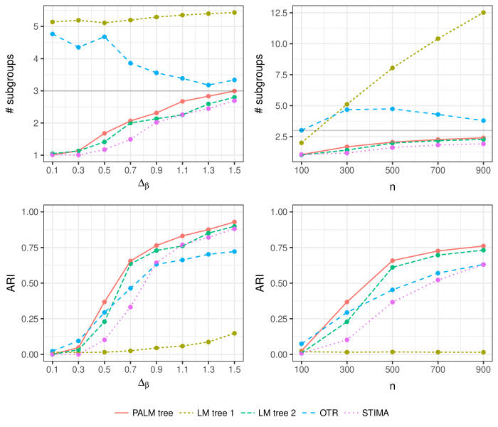
Figure 2: Mean number of subgroups and mean ARI for varying $\Delta_{\beta}$ and number of observations (Question 3.1).

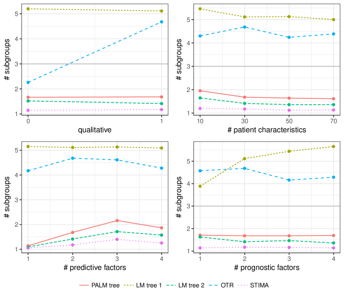
Figure 3: Mean number of subgroups for varying types of subgroups (quantitative/qualitative), number of patient characteristics, predictive factors and prognostic factors (Question 3.1).

To investigate whether the correct subgroups are captured by the different methods, we looked at the number of subgroups found as well as the adjusted Rand index (ARI, Hubert and Arabie, 1985; Milligan and Cooper, 1986). The ARI measures how well the retrieved subgroups fit with the true underlying subgroups. If the subgroups found are similar to the true subgroups the ARI will have a value up to 1. If the subgroups are only as good as a random group assignment the ARI is 0. If there is systematic missclassification, the ARI can also be negative.

The first row of Figure 2 shows the mean number of selected subgroups over the 150 simulated data sets and their corresponding trees for differing distances between treatment effects $\Delta_{\beta}$ and differing numbers of observations $n$. This means we are looking at the case where all variables are kept at the standard value except $\Delta_{\beta}$ or $n$ respectively. The second row shows the corresponding ARI. The similarity between the PALM tree and LM tree 2 algorithms is obvious. For both the number of subgroups and the ARI the results are very similar, although PALM tree is slightly better. Both algorithms get steadily closer to the optimal solution with increasing $\Delta_{\beta}$ as well as with increasing number of observations. LM tree 1 performs badly because it approximates the linear relation between the prognostic factors and the response with splits in the data. This is also the reason why with increasing $n$ the number of subgroups increases. This effect muffles the grouping with respect to the treatment effect, even if it gets less with increasing $\Delta_{\beta}$. The number of subgroups found for OTR is on average greater than the actual number of subgroups (3 for the given scenarios in Figure 2). The variability of the number of subgroups for OTR is very high (with a maximum of 20 subgroups). The true subgroups are not captured as well as with PALM tree and LM tree 2. The ARI for OTR is lower than the ARI of PALM tree and LM tree 2 except for very low values of $\Delta_{\beta}$ and $n$, which can be explained by the fact that the model-based trees use statistical significance tests and CART does not. Even though the pattern of STIMA in terms of the average number of subgroups appears similar to PALM tree and LM tree 2, on average the ARI is considerably lower, except for very large differences in treatment effects ($\Delta_{\beta}$).

Figure 3 shows the mean number of subgroups for the remaining simulation scenarios. The model-based trees and STIMA are not affected by the type of subgroup. OTR, however, is designed to find only qualitative subgroups and thus on average finds fewer groups when there are only quantitatively differing subgroups. For increasing number of patient characteristics, the model-based trees become more conservative and find slightly less subgroups, which is due to the correction for multiple testing (Bonferroni correction). OTR and STIMA do not change much in terms of average number of subgroups when the number of patient characteristics increases. With increasing number of predictive factors the number of subgroups should increase. The true number of subgroups is always the number of predictive factors $+~{}1$. The lower left panel of Figure 3 shows that this is not the case for any of the algorithms. The reason for this is the way of how we simulated the data. With an increasing number of predictive factors the subgroups get smaller and thus there is less power to find splits. The only algorithm that is strongly affected by the number of prognostic factors is LM tree 1, which corresponds to the fact that there are more linear terms to approximate through the tree structure.

3.2 How often are subgroups found even though there are none?

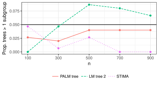
Figure 4: Proportion of trees with more than one subgroup for varying number of observations (Question 3.2). Black line at 0.05.

To investigate the type 1 error rate, i.e. the probability that subgroups are found even though there are none, we simulated data as above, but with no predictive factors. This means the treatment effect is the same for all patients. Figure 4 shows the behaviour of the methods with changing number of observations. LM tree 1 and OTR have a constant value of 1 here and are not visualised. Since LM tree 1 finds subgroups that have to do with the prognostic factors the “bad” performace exists by design. PALM tree is close to the expected $5\%$ significance level, as is LM tree 2. STIMA goes down to $0\%$ for 700 and 900 observations.

3.3 Is the correct treatment predicted to be better?

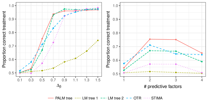
Figure 5: Proportion of observations in all trees where better treatment is correctly identified (Question 3.3).

The next measure we wanted to look at is the proportion of patients for which the better treatment is correctly identified. This is what OTR was designed to be good at and especially due to the way we simulated data (with a simple interaction) OTR can be expected to perform well. Figure 5 shows the proportion of patients for which the better treatment is correctly identified for the scenarios with varying difference between treatment effects $\Delta_{\beta}$ and varying number of predictive factors. When the difference between treatment effects $\Delta_{\beta}$ is small it is difficult for all methods to predict the correct treatment regime. For $\Delta_{\beta}=0.1$ it is close to random guessing. With increasing $\Delta_{\beta}$ all methods get better. The performance of PALM tree, LM tree 2, OTR and STIMA is similar. The four methods also behave similarly with a changing number of predictive factors. The treatment regime prediction is globally worst on average when there is one predictive factor. This results from the fact that often no split is found in this case (see Figure 3). In cases where the methods decide not to split at all, this leads by simulation design to a proportion of $50\%$ correctly-defined treatment regimes. The proportion of patients for which the correct treatment is predicted to be the better treatment improves in cases of two or three predictive factors and gets worse with four predictive factors. With more complex and smaller subgroups it becomes more difficult for the algorithms to retrieve the correct subgroup structure and to estimate the treatment effect. Note, however, that shape of the shape of the curves in the right panel of Figure 5 is very specific for the simulation settings here. Figure 9 shows the results for other scenarios. For example, for $\Delta_{\beta}=1.5$ and 300 observations in a setting with qualitative treatment differences, the best performace of PALM tree is with only one predictive factor and decreases from there. The performance of all algorithms is well in quantitative settings. OTR is the only algorithm that goes down to only 80% correctly defined treatment regimes in settings with 100 observations.

3.4 How good is the treatment effect estimate?

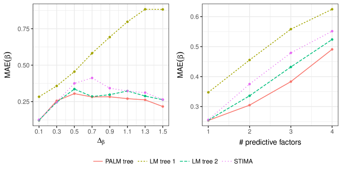
Figure 6: Mean absolute difference between true and estimated treatment effect (mean absolute error, MAE; Question 3.4).

Estimating or even predicting the correct treatment effect is the most essential part of subgroup analysis. Even if one treatment is better than the other, clinicians need to know if the difference is relevant. The evaluation of the treatment effect estimate can only be done for the model-based recursive partitioning methods and STIMA since OTR is only designed to produce binary decision rules. The measure used to evaluate the treatment effect estimate is the mean absolute difference between true and estimated treatment effect (mean absolute error, MAE). Figure 6 shows the MAE for the scenarios of varying $\Delta_{\beta}$ and varying number of predictive factors. The error is smallest for all three methods when the difference in treatment effect is lowest ($\Delta_{\beta}=0.1$), because even if the chosen subgroups are wrong, the estimated treatment effect will likely be close to the true and very similar treatment effects. In this sense it is not a disadvantage that PALM tree, LM tree 2 and STIMA often do not split into subgroups at all. In fact, it may even be an advantage, as the treatment effect estimate is then calculated based on a larger data set and is less affected by random variability. The effect of the small treatment difference gets less as the difference increases. However, as the it increases, finding the correct subgroups becomes easier and the error decreases. At the same time finding the correct subgroups becomes easier and slowly the error decreases again for PALM tree, LM tree 2 and STIMA. For this effect to be visible for LM tree 1, one would have to have larger treatment effects, fewer prognostic factors and/or more observations, given the large effect of the prognostic factor (see Figure 11 in the Appedix). With an increasing number of predictive factors the mean absolute error in treatment effect increases. The shape of the curve in Figure 6 looks very different to the one in Figure 5, even though they address similar questions, but the more true predictive factors exist in the given simulation scenario the harder it is for the methods to predict the treatment effect. This suggests that simply knowing the more effective treatment does not tell the whole story. This is supported across simulation scenarios (compare Figures 9 and 10).

4 Illustration: Treatment differences in mathematics exam

The Mathematics 101 course for first-year business and economics students at Universität Innsbruck gives an introduction to mathematical analysis, linear algebra, financial mathematics, and probability calculus. Students are assessed by biweekly online tests during the semester and a written exam at the end. The exam consists of 13 single-choice questions with 5 answer alternatives, one of which is correct. Students who answer more than 60 percent of the questions correctly pass the course. The percentage of successful online tests captures math ability of the students and is a known predictor for success in the final exam.

The data contains the exam results of 729 students (out of 941 who originally registered for the course) for the fall semester in 2014/15. Due to limited availability of seats in the exam room, the students were asked to select a group, where the first group wrote the exam in the morning and the second group right after the first group finished. The two groups received slightly different questions on the same topics covering the scope of the course. We are interested in whether the exam is fair in the sense that it is on average equally hard or difficult for the two groups. In other words we want to find out whether there is a “treatment effect” with the different selection of exam questions in the two groups corresponding to the “treatments”. As a first rather naive check we consider a simple one-way regression model for the percentage of correct answers by group, as reported in the first column of Table 2. This yields an expected percentage of 57.6 for a student in group 1 and a difference of 2.33 percentage points for students in group 2. Thus, the model finds only a small drop in the percentage of correctly solved answers and the corresponding confidence interval includes a zero change.

However, in this first model we have neglected the influence of the students’ ability which is particularly relevant here because the students could freely choose their exam group. Therefore, there might have been self-selection of more (or less) able students into the first (or second) group. To account for such ability effects in the model we include the percentage of points from the previous online tests that captures the students’ ability and preparation. As shown in the second column of Table 2 this variable is indeed strongly associated with the exam results, where one additional percentage point in the online tests leads to additional 0.86 expected percentage points in the written exam. More importantly, the group effect increases to 4.37 and the corresponding confidence interval does not include zero anymore. Despite the increase in the group effect, the absolute size of the group difference is still moderate corresponding to about half an exercise out of 13.

To explore the size of the treatment effect for the group differences further, we consider the possibility that this may vary across subgroups of students. Known student characteristics that may lead to such subgroups here are gender, the number of semesters the student has already been studying, the number of times the student has already attempted the exam, the type of study (three year bachelor program vs. four year diploma program) and also the ability/preparation as captured by percentage of successful exercises in the online tests. Since the test results in the online tests during the semester are known to have an important direct effect on the performance in the exam, the test parameter is included in the PALM tree. Figure 7 shows the resulting PALM tree with the segmented local group effect while adjusting for a global online tests effect. The strongest parameter instability is associated with the number of attempts and the group of students in the first attempt are split a second time by the percentage from the online tests. Two of the resulting subgroups (node 3 and 5) exhibit only very small group differences but in node 4 the second group obtained clearly a lower response percentage. This node is the smallest subgroup found and encompasses the highly able students taking the course for the first time. For this subsample the treatment effect is about 14 percentage points, which means that the students in the second batch solved about two exercises less than those in the first batch.

Overall this clearly conveys the strength of the PALM tree method: Especially in situations where the coefficient of interest is modest in a main-effects model and where further covariates are available whose influence on the main model parameters is not obvious, the PALM tree is an attractive option to globally control for certain variables while searching for local effects in others. Note, however, that due to the forward selection of models/effects the resulting confidence intervals in the terminal nodes (Table 2 and Figure 7) should not be used for inference but interpreted as a measure of variability.

Table 2: Three models for the mathematics exam data. The response variable is the percentage of correctly solved exercises and the main covariat of interest are the treatment differences between the first and second exam group. Confidence intervals are given in brackets.

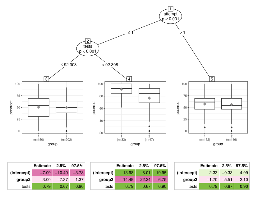
Figure 7: PALM tree for the percentage of correct answers explained by group differences while globally adjusting for ability (i.e., percentage of points obtained in previous online tests).

5 Discussion

Model-based trees are effective tools to identify subgroups in data which differ in terms of model parameters. PALM trees are special model-based trees where some parameters can be fixed globally for the entire sample and do not depend on the subgroup structure. Our simulation study has shown that in cases where there are such specified factors with a direct effect on the outcome, PALM trees reliably detect the correct subgroups while at the same time having a low probability of detecting subgroups when there are none. STIMA is a flexible and well performing competitor of model-based trees. The most important downside of STIMA is that it is very slow with in some instances single trees taking hours to compute (see Appendix B). Moreover, it has to be taken with a grain of salt that the R package “stima” is not actively maintained on the Comprehensive R Archive Network. Although optimal treatment regimes (OTR) perform comparably to PALM trees in terms of detecting the best treatment option in the given simulation study, PALM trees are typically better at recovering a parsimonious tree capturing the underlying subgroup structure. This makes PALM tree results easier to interpret and to communicate to practitioners, which we believe is an important advantage in many applications. Moreover, the simulation study clearly showed the effect of misspecifications in global vs. local effects in PALM trees. While it is important to correctly identify the variables with additive effects (LM tree 1 vs. LM tree 2 or PALM tree), it is not so important to correctly identify whether these additive effects are global or local (LM tree 2 vs. PALM tree). However, by reducing the number of tests in the split procedure and focusing only on certain relevant model parameters, some power and efficiency can be gained from selecting a suitable PALM tree.

PALM trees allow exploring and questioning results of (generalised) linear models. The PALM tree analysis of the Mathematics 101 exam showed that a linear model regressing the percentage points of correct anwers on the group and earlier test results is too simple. Only for a relatively small subgroup of students who attempted the exam for the first time and who showed good performance during the semester it did make a difference whether they attempted the exam in the first or second group.

Although large parts of this manuscript focus on subgroup analyses in clinical trials, PALM trees can also be applied in a wide range of other applications as well – e.g., in the social sciences as shown in the mathematics exam application case study.

Computational details

Open-source implementations of the model-based tree algorithms LM tree and GLM tree are available in the partykit package (Hothorn and Zeileis, 2015, functions lmtree() and glmtree()). The PALM tree algorithm is available in the palmtree package (Seibold et al, 2017, function palmtree()). OTR is available in package DynTxRegime (Holloway et al, 2015). The STIMA implementation has been archived on CRAN but can still be downloaded from https://cran.r-project.org/src/contrib/Archive/stima/. Simulations were conducted using the batchtools package (Lang et al, 2017).

The manuscript including simulation study and application can be reproduced using the supplementary online material.

Appendix A Full factorial simulation

The simulation study described in Section 3 takes a ceteris paribus approach and varies one simulation variable at a time while keeping the others at a standard value. We did an additional simulation study where we vary all variables, which leads to $8\cdot 5\cdot 2\cdot 4\cdot 4\cdot 4=5120$ (see Table 1) different scenarios. For each scenario we simulated two data sets and ran all algorithms on each. In the following we show a small selection of interesting graphics based on the simulations. For the full results of the simulation studies we refer to the online material.

Figure 8 shows the marginal results of the ARI for $\Delta_{\beta}$, the number of predictive factors, the number of observations and quantitative versus qualitative interactions. We average over the other simulation variables and the two repetitions. For sake of easy visualisation, we restrict the plotted variable to few levels. Similarly Figures 9 and 10 show the marginal results of the proportion of correct treatment assignment and mean absolute error in estimated treatment effect for the number of predictive factors, $\Delta_{\beta}$, the number of observations and quantitative versus qualitative interactions. Figure 11 shows the results for the MAE for $n=900$ and one prognostic factor to show when LM tree 1 starts to improve (see Section 3.4).

Figure 8 shows that PALM tree can handle simple subgroups with one predictive factor even when the number of observations is low, but the difference in treatment effects must be reasonably high. All other algorithms perform worse, with LM tree 2 and STIMA being the strongest competitors in the low-n-scenarios. OTR performs reasonably well if qualitative subgroups are present. For $n=500$ the performance of PALM tree rises already at lower levels of $\Delta_{\beta}$. The performance of PALM tree and LM tree 2 is very similar and STIMA also performs well. By design OTR ignores any non-qualitative subgroups.

When quantitative treatment subgroups exist, all methods are good at deciding the correct treatment regime (see Figure 9), especially when the number of observations is reasonably high (300). With $n=100$ PALM tree, LM tree 2, STIMA and even LM tree 1 still perform very well. OTR is the weakest competitor here. With low numbers of observations ($n=100$), low treatment effect differences ($\Delta_{\beta}=0.5$) and qualitative differences, the performance of all algorithms is close to random guessing (0.5), irrespective of the number of predictive factors. With higher $\Delta_{\beta}$ PALM tree performs reasonably well, followed by LM tree 2, STIMA and OTR (order depending on the number of predictive factors). For $n=300$ and $\Delta_{\beta}=0.5$ STIMA and LM tree 1 perform worst, but STIMA catches up with the other algorithms when $\Delta_{\beta}=1.5$, whereas LM tree 1 stays at the bottom. Section 3.3 discusses these results in the context of the results in the star-like simulation study.

Section 3.4 already partly discussed Figures 10 and 11. Figure 10 shows that across different scenarios the MAE increases with increasing number of predictive factors. PALM tree is among the best performers everywhere. In comparison to the other algorithms it performs particularly well in low-n-qualitative scenarios whith $\Delta_{\beta}=1.5$.

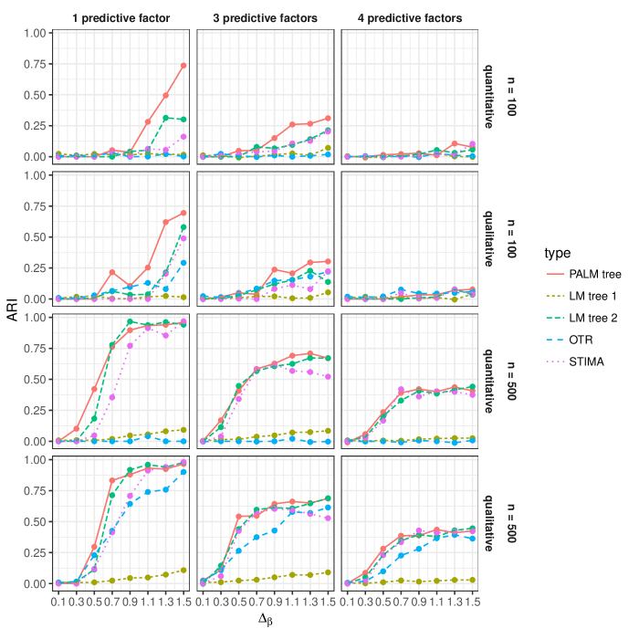
Figure 8: Mean ARI in the full factorial design with two simulated data sets per design (Question 3.1).

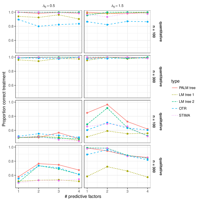
Figure 9: Proportion of observations in all trees where better treatment is correctly identified in the full factorial design with two simulated data sets per design (Question 3.3).

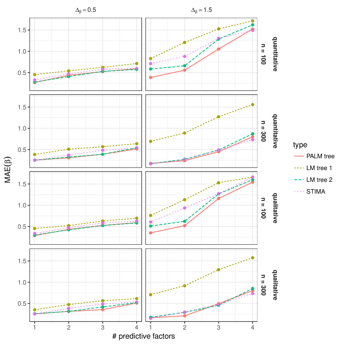
Figure 10: Mean absolute difference between true and estimated treatment effect (mean absolute error, MAE) in the full factorial design with two simulated data sets per design (Question 3.4).

Figure 11: Mean absolute difference between true and estimated treatment effect (mean absolute error, MAE) in the full factorial design with two simulated data sets per design (Question 3.4). Limited data to scenarios with 900 observations and one prognostic factor.

Appendix B Computation times

The computation times for all methods except STIMA are very reasonable in these applications. For a summary of computation times in the full factorial desing see Table 3. STIMA reached a maximum of 17.4 hours and almost half the models took half an hour or longer.

Table 3: Quantiles of computation times per algorithm in seconds.

	0%	25%	50%	75%	100%
PALM tree	0	0	1	2	7
LM tree 1	0	1	1	2	5
LM tree 2	0	0	1	1	4
OTR	0	0	1	1	2
STIMA	3	233.5	1941	8646.5	62512

References

- Breiman et al (1984) Breiman L, Friedman J, Stone CJ, Olshen RA (1984) Classification and Regression Trees. Wadsworth
- Chen et al (2007) Chen J, Yu K, Hsing A, Therneau TM (2007) A partially linear tree-based regression model for assessing complex joint gene-gene and gene-environment effects. Genetic Epidemiology 31(3):238–251, 10.1002/gepi.20205
- Doove et al (2014) Doove LL, Dusseldorp E, Van Deun K, Van Mechelen I (2014) A comparison of five recursive partitioning methods to find person subgroups involved in meaningful treatment-subgroup interactions. Advances in Data Analysis and Classification 8(4):403–425, 10.1007/s11634-013-0159-x
- Dusseldorp et al (2010) Dusseldorp E, Conversano C, Van Os BJ (2010) Combining an additive and tree-based regression model simultaneously: Stima. Journal of Computational and Graphical Statistics 19(3):514–530, 10.1198/jcgs.2010.06089
- Fokkema et al (2017) Fokkema M, Smits N, Zeileis A, Hothorn T, Kelderman H (2017) Detecting treatment-subgroup interactions in clustered data with generalized linear mixed-effects model trees. Behavior Research Methods In press
- Hajjem et al (2011) Hajjem A, Bellavance F, Larocque D (2011) Mixed effects regression trees for clustered data. Statistics & Probability Letters 81(4):451–459, 10.1016/j.spl.2010.12.003
- Holloway et al (2015) Holloway ST, Laber EB, Linn KA, Zhang B, Davidian M, Tsiatis AA (2015) DynTxRegime: Methods for Estimating Dynamic Treatment Regimes. URL https://CRAN.R-project.org/package=DynTxRegime, R package version 2.1
- Hothorn and Zeileis (2015) Hothorn T, Zeileis A (2015) partykit: A modular toolkit for recursive partytioning in R. Journal of Machine Learning Research 16:3905–3909, URL http://jmlr.org/papers/v16/hothorn15a.html
- Hothorn et al (2006) Hothorn T, Hornik K, Zeileis A (2006) Unbiased recursive partitioning: A conditional inference framework. Journal of Computational and Graphical Statistics 15(3):651–674, 10.1198/106186006X133933
- Hubert and Arabie (1985) Hubert L, Arabie P (1985) Comparing partitions. Journal of Classification 2(1):193–218, 10.1007/BF01908075
- Italiano (2011) Italiano A (2011) Prognostic or predictive? It’s time to get back to definitions! Journal of Clinical Oncology 29(35):4718–4718, 10.1200/JCO.2011.38.3729
- Lang et al (2017) Lang M, Bischl B, Surmann D (2017) batchtools: Tools for R to work on batch systems. The Journal of Open Source Software 2(10), 10.21105/joss.00135
- Lipkovich et al (2016) Lipkovich I, Dmitrienko A, D’Agostino RB (2016) Tutorial in biostatistics: Data-driven subgroup identification and analysis in clinical trials. Statistics in Medicine 10.1002/sim.7064
- Loh (2002) Loh WY (2002) Regression trees with unbiased variable selection and interaction detection. Statistica Sinica 12(2):361–386, URL http://www.stat.sinica.edu.tw/statistica/oldpdf/a12n21.pdf
- Mbogning and Toussile (2015) Mbogning C, Toussile W (2015) GPLTR: Generalized Partially Linear Tree-Based Regression Model. URL https://CRAN.R-project.org/package=GPLTR, R package version 1.2
- Milligan and Cooper (1986) Milligan GW, Cooper MC (1986) A study of the comparability of external criteria for hierarchical cluster analysis. Multivariate Behavioral Research 21(4):441–458, 10.1207/s15327906mbr2104_5
- Seibold et al (2016) Seibold H, Zeileis A, Hothorn T (2016) Model-based recursive partitioning for subgroup analyses. International Journal of Biostatistics 12(1):45–63, 10.1515/ijb-2015-0032
- Seibold et al (2017) Seibold H, Hothorn T, Zeileis A (2017) palmtree: Partially additive (generalized) linear model trees. URL https://CRAN.R-project.org/package=palmtree, R package version 0.9-0
- Sela and Simonoff (2012) Sela RJ, Simonoff JS (2012) RE-EM trees: A data mining approach for longitudinal and clustered data. Machine Learning 86(2):169–207, 10.1007/s10994-011-5258-3
- Sies and Van Mechelen (2017) Sies A, Van Mechelen I (2017) Comparing four methods for estimating tree-based treatment regimes. The International Journal of Biostatistics Online First, 10.1515/ijb-2016-0068
- Zeileis and Hornik (2007) Zeileis A, Hornik K (2007) Generalized M-fluctuation tests for parameter instability. Statistica Neerlandica 61(4):488–508, 10.1111/j.1467-9574.2007.00371.x
- Zeileis et al (2008) Zeileis A, Hothorn T, Hornik K (2008) Model-based recursive partitioning. Journal of Computational and Graphical Statistics 17(2):492–514, 10.1198/106186008X319331
- Zhang et al (2012) Zhang B, Tsiatis AA, Davidian M, Zhang M, Laber E (2012) Estimating optimal treatment regimes from a classification perspective. Stat 1(1):103–114, 10.1002/sta.411