Tangent bundle geometry from dynamics: application to the Kepler problem

Abstract

In this paper we consider a manifold with a dynamical vector field and inquire about the possible tangent bundle structures which would turn the starting vector field into a second order one. The analysis is restricted to manifolds which are diffeomorphic with affine spaces. In particular, we consider the problem in connection with conformal vector fields of second order and apply the procedure to vector fields conformally related with the harmonic oscillator (f-oscillators) . We select one which covers the vector field describing the Kepler problem.

1 Introduction

Often, for various reasons (reduction, quantum-to-classical transition, reparametrization, statistical models, etc) we are dealing with dynamical systems on carrier spaces where a clear identification of “positions” and “velocities” (or “momenta”) need not be available. It is therefore meaningful to investigate if and when it is possible to identify “positions” and “velocities” or “momenta” Equivalently, if we are given a dynamical system described by a vector field $\Gamma$ on some carrier manifold $M$, we would like to investigate whether and when the carrier manifold may be given a tangent bundle structure which turns the given vector field into a second order vector field. This could also be a way, for instance, to investigate the inverse problem of the calculus of variations in a greater generality.

In order to avoid topological obstructions, we shall consider in this paper only the simplest situation: $M=\mathbb{R}^{2n}$. If we are aiming, for instance, at the Lagrangian case, our goal would be to identify a submanifold $\mathbb{R}^{n}\subset M$ which would allow to write $M\approx T\mathbb{R}^{n}$, in such a way that $\Gamma$ becomes a second order differential equation vector field with respect to the tangent bundle structure.

The simplest example is provided by the free particle in $\mathbbm{R}^{3}$, even though it is described by the free Lagrangian

$${L}=\frac{1}{2}\langle\dot{\vec{r}},\dot{\vec{r}}\rangle,$$

the reduction of the dynamics along the radius is not described by the “reduced Lagrangian” (see [2]) but a simple minded reduction would have the wrong sign in the “centrifugal potential”. Therefore the Lagrangian description of the reduced dynamics needs to be found by means of the inverse problem. In this way we would find the correct “minus sign” in the centrifugal potential.

In other reductions the reduced carrier space may turn out to have odd dimension and therefore the identification of “positions” and “velocities” would not be possible. Analogous situations may arise within the quantum-to classical transition where the classical limit need not be directly a phase space. This would occur, for instance for particles with spin.

A similar situation was studied from the Hamiltonian perspective in [21] under the name of “$Q$-dynamical systems”. Such objects were introduced as the flow under the diffeomorphism group of a Hamiltonian vector field $X$ with respect to a given symplectic form $\omega$. This starting symplectic form was considered to be the canonical symplectic form of the cotangent bundle $T^{*}Q$ for a given choice of the configuration space $Q$. However, by performing a generic transformation by means of a non-canonical diffeomorphism which would be a symmetry for the dynamics, as the symplectic structure would not be preserved, we would loose the separation between “positions” and conjugate momenta.

In conclusion we would face the problem of reconstructing a tangent or a cotangent bundle structure after a transformation by a generic diffeomorphism which would not be a tangent bundle automorphism.

It should be noticed that this situation would already occur from one Galileian frame to a different one, expressing the fact that “zero velocity” or “zero motion” of the tangent bundle cannot have an absolute meaning. Indeed, let us consider for simplicity the vector field $\Gamma$ of a free motion on $\mathbbm{R}^{2n}$. Thus, we assume that there exists coordinate functions $\{\eta^{j},\xi^{k}\}$ satisfying

$$\mathcal{L}_{\Gamma}\eta^{j}=\xi^{j};\qquad\mathcal{L}_{\Gamma}\xi^{j}=0\quad\forall j.$$ (1)

Clearly, if we choose as coordinates

$$\eta^{\prime k}=\eta^{k}+f^{k}(\vec{\xi}),\qquad\xi^{\prime j}=\xi^{j}$$ (2)

for $f^{k}$ arbitrary smooth functions, the coordinates $(\eta^{\prime},\xi^{\prime})$ share the same properties as the original ones with respect to $\Gamma$. Hence, we see that there is some freedom in the choice of coordinates of the submanifold representing the “positions”. If the functions $\xi^{j}$ are such that the set $\vec{\xi}=0$ defines a smooth submanifold of $\mathbbm{R}^{2n}$, say $Q$, then our original manifold is diffeomorphic with $TQ$. But Galileian relativity would change the zero section of that bundle, since velocities would be changed by a constant vector. We conclude thus that for a free motion to be modeled as a SODE and to take into account Galilean relativity, we must consider different tangent bundle structures, one particular structure being associated with every chosen frame.

As it is well-known a tensorial description of a tangent bundle structure is provided by two tensor fields, $S$, soldering (1,1) tensor field, and a Liouville vector field, also called “partial linear structure”. More specifically, it is known [1, 3, 4, 5, 9, 12, 13] that the geometry of a tangent bundle is encoded in two tensors:

• the vertical endomorphism $S$, a $(1,1)$ tensor defined on the tangent bundle $TM$ on a manifold $M$ which in the natural coordinates $(q^{k},v^{k})$ reads

  $$S=dq^{k}\otimes\frac{\partial}{\partial v^{k}},$$ (3)

• and the Liouville vector field, which encodes the dilations along the fibers and hence their linear structures. The corresponding local expression reads

  $$\Delta=v^{k}\frac{\partial}{\partial v^{k}}.$$ (4)

By construction, $S^{2}=0$ and ${\mathcal{L}}_{\Delta}S=-S$. Both tensors allow us to define Second Order Differential Equations (SODE) to be those vector fields $X\in\mathfrak{X}(TM)$ which satisfy

$$S(X)=\Delta.$$ (5)

This relation shows very clearly that the condition for a vector field to be a SODE depends on both $S$ and $\Delta$.

A translation along each fiber of the tangent bundle would not alter the soldering tensor but would change the dilation vector field. The vector field $\Delta=(v^{i}+c^{i}(q))\,\partial/\partial v^{i}$ also satisfies $\mathcal{L}_{\Delta}S=-S$, but then the condition $S(\Gamma)=\Delta$ would not hold true for vector fields which were second order with respect to the previous structure.

Furthermore, given a regular Lagrangian function $L$, Euler-Lagrange equations which are implicit differential equations, may be solved in terms of the solutions of a second order vector field $\Gamma$, if it exists, that satisfies the following equation

$${\mathcal{L}}_{\Gamma}\theta_{L}-dL=0,$$ (6)

where $\theta_{L}$ is the 1-form defined by the dual map of the vertical endomorphism (denoted by $S^{*}$) as

$$\theta_{L}=S^{*}(dL)=dL\circ S.$$ (7)

The main result can be summarized as follows (see [1, 9]):

Theorem 1.

A differential manifold $M$ may be endowed with a tangent bundle structure if and only if there exist a complete vector field $\Delta$, whose zeros define a submanifold $Q$ of $M$, and a $(1,1)$ tensor field $S$ satisfying the following conditions:

• $\mathrm{Ker}S=\mathrm{Im}S$, i.e. $S^{2}=0$

• $\Delta\in\mathrm{Im}S$, what implies that $S(\Delta)=0$

• ${\mathcal{L}}_{\Delta}S=-S$

• $N_{S}=0$, where $N_{S}$ stands for the Nijenhuis torsion for $S$

• the limit of the flow of $\Delta$, $\lim_{t\to-\infty}\Phi_{t}^{\Delta}(p)$ exists for any $p\in M$.

$S$ and $\Delta$ uniquely determine a tangent bundle structure for $M$. Indeed, it is possible to identify the submanifold $Q$ as the base manifold which makes $M$ diffeomorphic to $TQ$. When considering adapted coordinates $(q^{i},v^{j})$ on this $TQ$, the local expressions of the tensors become (3) and (4).

Different choices of these tensors define different tangent bundle structures for the manifold $M$. In this paper we are going to study the general conditions to determine a suitable tangent bundle structure that makes a given vector field $\Gamma$ a SODE on $M=\mathbbm{R}^{2n}$.

We will also focus our attention on two particular situations where such a construction produces interesting properties: the definition of a new vector field conformal to the given $\Gamma$ (as for instance when we try to regularize it to make it complete) and the deformation of a vector field by a function, in particular in the form of an $f$–oscillator introduced in [19]. As an important application, we will consider the regularization of the Kepler problem, and we will see that the redefinition of the tangent bundle structures will allow us to define a suitable diffeomorphism of its space of motions and the space of motions of a $f$–oscillator. Such mapping circumvents the obstruction arising from the energy-period theorem (see [10, 11, 17]) to identify both systems at the phase-space level.

The scheme of the paper is as follows. Section 2 introduces the case of the reparametrization of a vector field and the type of conformal factor required to make the reparametrized vector field complete. Finally, we will discuss how this process affects the set of periodic orbits. In Section 3 we will consider the deformation of vector fields by introducing the notion of $f$–oscillator. In particular, we introduce for the first time here the Lagrangian version of that construction and show how the resulting system takes also the form of a conformal vector field with the conformal factor being a function of the oscillator energy. Then, Section 4 presents the main result of the paper: given a vector field $\Gamma^{\prime}$ on some carrier space $M$, is it possible to define a suitable tangent bundle structure on $M$ which makes $\Gamma^{\prime}$ a SODE? We will obtain the generic properties for that to happen and present some relevant examples. In particular we study the case where $\Gamma^{\prime}$ is a conformal vector field with respect to a SODE vector field in some original tangent bundle structure and look for the conditions for the existence of a new structure with respect to which the new vector field $\Gamma^{\prime}$ is a SODE. We will apply this to the regularized Kepler problem and the $f$–oscillator problem and we will prove that the new SODE vector fields are formally identical and equal to a harmonic oscillator with a frequency which depends on the point. Finally, in Section 5 we will prove that the similarities of the resulting SODE vector fields of two systems allow us to define an invertible mapping of the corresponding spaces of motion and apply that to the case of the Kepler problem and the $f$–oscillator. Thus we will prove that it is possible to identify a suitable deformation function $f$ to deform a harmonic oscillator in such a way that the resulting SODE vector field has the same frequencies as the SODE of the regularized Kepler problem, allowing us to define a one-to-one relation of their respective motion spaces. Finally, Section 6 summarizes the main results of the paper and discuss some of its possible extensions.

2 Conformally related vector fields: reparametrization and completeness

The need for reparametrization of a vector field may come from different situations. One possible case is the need of defining a complete vector field associated to a given dynamics, as it happens, for instance, in the case of the closed orbits of the Kepler problem. Another situation requiring regularized vector fields is the case of quantization, where systems whose classical dynamical vector field is not complete may give rise to quantum Hamiltonian operators which are not self-adjoint and therefore nonphysical (see [26]). In this case the appropriate identification of the corresponding conjugate variables becomes very important.

Hence in this Section we are going to discuss a few properties of the regularization mechanism, and, in particular, the implications at the level of the period of the orbits of the vector fields, which is our main concern.

2.1 Definition and effects on tensors

The notion of conformally related differential operators is of great importance in many areas of Physics. We will summarize now the most relevant ones for vector fields, and we address the interested reader to the work by Palais [22] or to [1] for more details.

We say that two vector fields $X$ and $\Gamma$ on a differential manifold $M$ are conformally related vector fields if there exists a nowhere vanishing differential function $f\in C^{\infty}(M)$ such that $\Gamma=fX$. This defines an equivalence relation on the set of vector fields of a differential manifold. The dynamics associated to $\Gamma$ is very similar to the dynamics associated to $X$, but it also has some interesting differences. It is straightforward to prove, for instance, that $X$ and $\Gamma$ admit the same algebra of constants of the motion. Indeed, a function $g\in C^{\infty}(M)$ is a constant of motion for $X$, i.e ${\mathcal{L}}_{X}g=0$, if and only if $\mathcal{L}_{\Gamma}g=0$, because ${\mathcal{L}}_{\Gamma}g={\mathcal{L}}_{fX}g=f{\mathcal{L}}_{X}g$.

However, the algebra of invariant tensor fields under $X$ does not coincide with the algebra of invariant tensor fields under $\Gamma$. Indeed, if we consider for instance a 1–form $\alpha\in\bigwedge^{1}(M)$ which is preserved by the vector field $X$, it may happen that $\Gamma$ does not preserve it, because

$${\mathcal{L}}_{\Gamma}\alpha=(di_{\Gamma}+i_{\Gamma}d)\alpha=d(fi_{X}\alpha)+f(i_{X}d\alpha)=(i_{X}\alpha)\,df+f{\mathcal{L}}_{X}\alpha,$$ (8)

and the term $(i_{X}\alpha)\,df$ may be different from zero even if ${\mathcal{L}}_{X}\alpha=0$. Analogously, if we consider a 2-form as $\alpha\wedge\beta$ for $\alpha,\beta\in\Lambda^{1}(M)$, we obtain

$$\mathcal{L}_{\Gamma}(\alpha\wedge\beta)=(\mathcal{L}_{\Gamma}\alpha)\wedge\beta+\alpha\wedge(\mathcal{L}_{\Gamma}\beta)=(i_{X}\alpha)\,df\wedge\beta+(i_{X}\beta)\,\alpha\wedge df+f(\mathcal{L}_{X}(\alpha\wedge\beta)),$$ (9)

and then $\mathcal{L}_{X}(\alpha\wedge\beta)=0$ does not imply $\mathcal{L}_{\Gamma}(\alpha\wedge\beta)=0$.

If we consider the case of a vector field, we find similarly:

$${\mathcal{L}}_{\Gamma}Y={\mathcal{L}}_{fX}Y=[fX,Y]=-Y(f)X+f[X,Y],\quad\forall Y\in\mathfrak{X}(M),$$ (10)

and then $\mathcal{L}_{X}Y=0$ does not imply $\mathcal{L}_{\Gamma}Y=0$.

In case of a bivector field $Y\wedge Z$, for any $Y,Z\in\mathfrak{X}(M)$, the situation is similar, because

$${\mathcal{L}}_{\Gamma}(Y\wedge Z)=({\mathcal{L}}_{\Gamma}Y)\wedge Z+Y\wedge({\mathcal{L}}_{\Gamma}Z)= -Y(f)X\wedge Z-Z(f)Y\wedge X+$$

$$f({\mathcal{L}}_{X}Y\wedge Z+Y\wedge{\mathcal{L}}_{X}Z)$$

$$= \left(Y(f)Z-Z(f)Y\right)\wedge X+f({\mathcal{L}}_{X}(Y\wedge Z))$$ (11)

which shows that ${\mathcal{L}}_{X}(Y\wedge Z)=0$ does not imply $\mathcal{L}_{\Gamma}(Y\wedge Z)=0$.

The extension to more general tensors is straightforward. We notice that the conformal factor has consequences on the invariance properties of tensors fields, however these changes are simple to compute. This fact will be important in the following, since we will need to redefine the geometrical structures of $M$ to define new ones which are preserved by the vector field $\Gamma$.

It is also immediate that the orbits of vector fields $X$ and $\Gamma$ coincide. Indeed vector fields $X$ and $\Gamma$ are tangent to the same curves, the only difference being the parametrization chosen. Therefore we can understand the conformal factor as a kind of reparametrization of the curves. Consider an integral curve $x(t)$ of $X$ parametrized by $t\in I\subset\mathbb{R}$, i.e.

$$\frac{dx(t)}{dt}=X(x(t)),$$ (12)

and let $s(t)$ be a solution of the differential equation

$$\frac{ds}{dt}=f(x(t)),$$ (13)

which defines a good reparametrization because $f$ is of a constant sign. If we consider the condition for the curve $x$ to be an integral curve of the vector field $\Gamma$ we find:

$$\frac{dx(t)}{dt}=\Gamma(x(t))=f(x(t))X(x(t)).$$ (14)

It is immediate to see that by considering the reparametrization $s(t)$, the flow satisfies:

$$\frac{dx(s)}{ds}=X(x(s)).$$ (15)

Therefore the integral curves of $X$ and $\Gamma$ are the same submanifolds of $M$, but with a different parametrizations.

2.2 Completeness of a conformally-related vector field

In particular, we shall be interested in a conformally related vector field $\Gamma=fX$ which is complete, while $X$ is not. Such a construction can be used in any paracompact manifold. Indeed, given a vector field $X$ on a paracompact manifold $M$, there always exists a strictly positive function $f\in{\mathcal{F}}(M)$, of the same differentiability class as $X$ such that $\Gamma=f\,X$ is a complete vector field.

To prove this assertion one notices that, due to the paracompactness of $M$, there exists a proper function $g\in{\mathcal{F}}(M)$ of class $C^{s}$ on $M$. Let us consider thus

$$f=\exp\left(-\left({\mathcal{L}}_{X}g\right)^{2}\right);\qquad\Gamma=fX$$ (16)

It is immediate that

$$|{\mathcal{L}}_{\Gamma}g|=\left|\exp\left(-\left({\mathcal{L}}_{X}g\right)^{2}\right)({\mathcal{L}}_{X}g)\right|\leq 1$$ (17)

on $M$. Therefore, if we denote by $\gamma$ an integral curve of the vector field $\Gamma$ defined on a bounded interval $I$, then

$$\frac{d}{dt}(g\circ\gamma)=({\mathcal{L}}_{\Gamma}g)\circ\gamma,$$ (18)

and hence

$$\left|\frac{d}{dt}(g\circ\gamma)\right|\leq 1,$$ (19)

on $I$. Then the image of $g\circ\gamma$ is bounded and hence the image of $\gamma$ is relatively compact.

2.3 Conformally related vector fields, Hamiltonian structures and periodic orbits

As we said above, the unparametrized orbits of two conformally related vector fields $X$ and $\Gamma=fX$ coincide, but, in general, the vector field $\Gamma$ will not preserve the same geometric structures as $X$. Therefore the reparametrization defined by function $f$ is not compatible with other properties, such as the fact of being Hamiltonian (unless $f$ is a central element of Poisson algebra, for the corresponding symplectic or Poisson structure ) or being a Second Order Differential Equation (if the manifold is a tangent bundle). We will see later that in a particular case the condition of being a SODE can be recovered by defining a new tangent bundle structure on the same manifold.

In case of Hamiltonian structures, if $X=X_{H}$ is a Hamiltonian vector field associated with a function $H\in C^{\infty}(M)$ on a symplectic manifold $(M,\omega)$, the vector field $\Gamma=fX_{H}$ is not a Hamiltonian vector field, unless

$$i_{\Gamma}\omega=i_{fX_{H}}\omega=fi_{{X_{H}}}\omega=f\,dH.$$ (20)

Instead, $\Gamma$ is just a conformally Hamiltonian vector field. The interest on conformally Hamiltonian vector fields comes from the possibility of relating their integral curves with those of the Hamiltonian vector fields via a reparametrization of the curves. In general the 1-form $f\,dH$ is not exact and $\Gamma$ is not a Hamiltonian vector field. Only if

$$df\wedge dH=0,$$

the vector field $\Gamma$ is Hamiltonian. But even in this case a transformation of this type cannot make $\Gamma$ complete if $X_{H}$ is not, because a function of the Hamiltonian re-scales the parameter by a different constant value along each curve.

Notice that these properties are meaningful from the physical point of view, since they are associated to quantities as the period of closed orbits. From the reparametrization relation we introduced above, we can consider the two vector fields $X$ and $\Gamma=fX$ and the a curve $\gamma$ satisfying

$$\frac{d\gamma(t)}{dt}=\Gamma(\gamma(t))=f(\gamma(t))X(\gamma(t)).$$ (21)

If we consider the case where $f$ is a constant of the motion (as it will happen for $f$–oscillators), $f(\gamma(t))=K$ is constant for all $t$. Thus we realize that the effect on the curve $\gamma$ is just that the dynamics associated to $\Gamma$ runs $K$ times faster (if $K>1$) than the dynamics associated to $X$. It is straightforward to prove from Equation (13) that, if the conformal factor function $f$ is constant along the curve, i.e.,

$$f(\gamma(t))=K,\quad\forall t$$ (22)

its period is scaled by $K^{-1}$.

Notice that, in general, this re-scaling may differ from curve to curve, and therefore we may have examples (e.g. the harmonic oscillator), which, once transformed by a conformal factor, produce a set of circumferences as integral curves but with periods which are different for each curve. Therefore they cannot be considered as orbits of $SO(2)$ or $U(1)$ but should be considered orbits of $\mathbb{R}$.

This result is relevant if we aim to relate two Hamiltonian systems with periodic orbits. It implies, for instance, that we cannot map smoothly the set of solutions of a system with constant period (as the harmonic oscillator) on the solutions of a system with non-constant period (as for instance the Kepler problem). It is possible though to relate both models via a family of mappings parametrized by the energy. Then, an orbit corresponding to a certain energy in the Kepler problem is covered by closed orbits of the harmonic oscillator, but the mapping is not global: another Kepler-orbit with a different energy is covered by oscillator-orbits by a different mapping with a different frequency (which depends on the energy). Still, from what we just learned above, we may also search for a suitable conformal factor function $f$ which is a constant of the motion for $X$, and that tunes the period of each orbit to make them match exactly the function $T(E)$ which the energy-period theorem predicts for the Kepler problem. This is precisely what the $f$–oscillator will do.

3 Deforming dynamical vector fields: $f$–oscillators

The notion of $f$–oscillator was introduced in [19] as a procedure to define nonlinear coherent states by deforming the Hamiltonian function of the isotropic harmonic oscillator. This transformation changes the energy-period relation and allows us to consider it as a candidate to relate systems with closed orbits which have different energy-period relations with respect to that of the harmonic oscillator. This property will prove to be essential in order to combine the results from Section 4.4 into a one-parameter family of orbits of four-dimensional harmonic oscillators, each one with a different frequency, that are in correspondence with the set of closed orbits of the three-dimensional Kepler problem.

3.1 The notion of $f$–oscillator

Let us consider then an isotropic harmonic oscillator defined in $n$–dimensions, i.e. the dynamics is defined on $\mathbb{R}^{2n}$, parametrized by Darboux coordinates $\{(q^{k},p_{k}\mid k=1,\cdots,n\}$ by the Hamiltonian function

$$H=\frac{1}{2}\sum_{k=1}^{n}(p_{k}^{2}+(q^{k})^{2}),$$ (23)

with respect to the canonical symplectic form

$$\omega=\sum_{k=1}^{n}dq^{k}\wedge dp_{k}.$$ (24)

The corresponding Hamiltonian vector field reads:

$$X_{H}=\sum_{k=1}^{n}\left(p_{k}\frac{\partial}{\partial q^{k}}-q^{k}\frac{\partial}{\partial p_{k}}\right)$$ (25)

The $f$–oscillator dynamics is defined by constructing a new Hamiltonian function $\bar{H}$, which is obtained as the image of the original $H$ by a function $f:\mathbb{R}\to\mathbb{R}$. Thus we consider

$$\bar{H}=f(H)=f\left(\frac{1}{2}\sum_{k=1}^{n}(p_{k}^{2}+(q^{k})^{2})\right)$$ (26)

This Hamiltonian function produces a Hamiltonian vector field with respect to the symplectic form (24):

$$X_{\bar{H}}=\left.\frac{df(\xi)}{d\xi}\right|_{{\xi=H}}\sum_{k=1}^{n}\left(p_{k}\frac{\partial}{\partial q^{k}}-q^{k}\frac{\partial}{\partial p_{k}}\right)=\left.\frac{df(\xi)}{d\xi}\right|_{{\xi=H}}X_{H}.$$ (27)

The resulting dynamics is no longer linear, although it still produces periodic orbits. The main difference with respect to Equation (25) is that the frequencies change from one to another level set of energy. Different orbits on different level sets will have thus different periods, depending on the value of the derivative of the function $f(H)$ when evaluated at the orbit. An important point which will be relevant later is the fact that the level sets of the $f$–energy (i.e. the set of points where $f(H)$ is constant) are $2n-1$ spheres, as it happens with the undeformed level sets. In particular the group $SU(n)$ will be again a symmetry group of our reparametrized Hamiltonian vector field. The deformation by the function $f$ affects only to the rate of change of the radius from one to another level set.

3.2 Lagrangian formulation of a $f$–oscillator

The concept of $f$–oscillator was designed for and within the Hamiltonian formalism. The original idea was to build a deformed dynamics which was Hamiltonian with respect to an alternative symplectic structure. We want to consider now an alternative point of view: we want to study whether we can define a deformed description of a Lagrangian dynamics in an analogous way. Thus consider the Hamiltonian of the harmonic oscillator (23) and the corresponding Lagrangian description defined by the Legendre transform:

$${\mathcal{F}}H:T^{*}\mathbbm{R}^{n}\to T\mathbbm{R}^{n}$$ (28)

where ${\mathcal{F}}H$ is defined as

$${\mathcal{F}}H:(q^{k},p_{k})\mapsto\left(q^{k},\frac{\partial H}{\partial p_{k}}\right),$$ (29)

which, in our case, is a global diffeomorphism.

The dynamical vector field

$$X_{H}=\sum_{k}\left(\frac{\partial H}{\partial p_{k}}\frac{\partial}{\partial q^{k}}-\frac{\partial H}{\partial q^{k}}\frac{\partial}{\partial p_{k}}\right)=\sum_{k}\left(p_{k}\frac{\partial}{\partial q^{k}}-q^{k}\frac{\partial}{\partial p_{k}}\right)$$ (30)

is mapped by ${\mathcal{F}}H_{*}$ onto the vector field $\Gamma\in\mathfrak{X}(T\mathbbm{R}^{n})$

$$\Gamma=\sum_{k}\left(v^{k}\frac{\partial}{\partial q^{k}}-q^{k}\frac{\partial}{\partial v^{k}}\right).$$ (31)

$\Gamma$ is a SODE and it represents the dynamical vector field whose integral curves are the solutions of the Euler-Lagrange equations for the Lagrangian function

$$L=\frac{1}{2}\sum_{k}\left((v^{k})^{2}-(q^{k})^{2}\right).$$ (32)

This vector field can be given a symplectic formulation if we write

$$i_{\Gamma}\omega_{H}=dE_{H},$$ (33)

where the symplectic form $\omega_{H}$ is the pullback of the canonical symplectic form $\omega$ on $T^{*}\mathbbm{R}^{n}$ by the inverse of ${\mathcal{F}}H$, i.e.,

$$\omega_{H}=(({\mathcal{F}}H)^{-1})^{*}\omega,$$ (34)

and the energy function $E_{H}$ is the pullback of the Hamiltonian function by ${\mathcal{F}}H^{-1}$:

$$E_{H}=({\mathcal{F}}H^{-1})^{*}(H)=\frac{1}{2}\sum_{k}\left((v^{k})^{2}+(q^{k})^{2}\right).$$ (35)

If we consider the $f$–oscillator dynamics associated to the function $H^{\prime}$ defined $\bar{H}$ in Equation (26) and the vector field corresponding to Equation (27), we know that the vector field $X_{H^{\prime}}$ is conformally related to $X_{H}$, $X_{H^{\prime}}=f^{\prime}X_{H}$. The image of the vector field $X_{H^{\prime}}$ under ${\mathcal{F}}H_{*}$ defines a new vector field $\Gamma^{\prime}\in\mathfrak{X}(T\mathbbm{R}^{n})$ which is written as

$$\Gamma^{\prime}={\mathcal{F}}H_{*}(X_{H^{\prime}})=f^{\prime}(E_{H})\Gamma,$$ (36)

which is Hamiltonian with respect to the symplectic form $\omega_{H}$ (Equation 34) and the function

$$E_{H^{\prime}}=({\mathcal{F}}H^{-1})^{*}(H^{\prime}),$$ (37)

i.e.,

$$i_{\Gamma^{\prime}}\omega_{H}=dE_{H^{\prime}}.$$ (38)

In conclusion we have proved that a $f$-oscillator, when described in a Lagrangian framework, corresponds to a vector field $\Gamma^{\prime}$ which is a conformal vector field with respect to a Harmonic oscillator vector field, the conformal factor being a function of the energy of the (undeformed) oscillator. We will see later on how the similarities with conformal vector fields can be used to obtain interesting properties of the deformations.

4 Alternative tangent bundle structures from dynamics

4.1 Defining the tangent bundle

From Theorem 1 we know that the tangent bundle structure is encoded in a pair of tensors satisfying some compatibility conditions. We can consider different tangent bundle structures in the same carrier space $M$ by choosing different pairs of tensor fields $(S,\Delta)$ in $M$ satisfying the properties above. It is obvious that by changing the tangent bundle structure will change the nature of vector fields on $M$ as SODE. Our goal now is to find a suitable pair $(\hat{S},\hat{\Delta})$ on the manifold $M=T\mathbbm{R}^{n}$ (the total manifold of the original tangent bundle) such that $\Gamma^{\prime}$ satisfies that

$$\hat{S}(\Gamma^{\prime})=\hat{\Delta}.$$ (39)

In order to do that we are going to choose $n$ functions $\{Q^{1},\cdots,Q^{n}\}$ of $M=T\mathbbm{R}^{n}$ which will play the role of the new coordinates, satisfying

$$(dQ^{1}\wedge\cdots\wedge dQ^{n})(p)\neq 0,$$ (40)

for each point of $B$ or, at least, on a dense submanifold $Q$ of $M$. These functions identify the base manifold of our new tangent bundle. Notice that the level set of these new coordinates must define a vector space, which will correspond to the tangent space at the point defined by the values of the coordinates. Now, having in mind the requirement of $\Gamma^{\prime}$ to be a SODE, we define:

$${\mathcal{V}}^{k}={\mathcal{L}}_{\Gamma^{\prime}}Q^{k},\qquad k=1,\cdots,n,$$ (41)

where the set of functions $\{{\mathcal{V}}^{1},\cdots,{\mathcal{V}}^{n}\}$ play the role of the new velocities. This, of course, implies that the coordinates must have the property that $\Gamma^{\prime}$ has no fixed points on the submanifold, i.e. $\Gamma^{\prime}(p)\neq 0$, $\forall p\in Q$. If all the velocity functions are functionally independent, the bundle structure is well defined and $\Gamma^{\prime}$ becomes a SODE with respect to the new structure. Thus we have to require that

$$dQ^{1}\wedge\cdots\wedge dQ^{n}\wedge d{\mathcal{V}}^{1}\wedge\cdots\wedge d{\mathcal{V}}^{n}\neq 0\qquad\forall p\in M.$$ (42)

In conclusion, the vector field $\Gamma^{\prime}$ will take the form:

$$\Gamma^{\prime}=\sum_{k}\left(\mathcal{V}^{k}\frac{\partial}{\partial Q^{k}}+\mathcal{F}^{k}\frac{\partial}{\partial\mathcal{V}^{k}}\right),$$ (43)

where

$$\mathcal{F}^{k}=\mathcal{L}_{\Gamma^{\prime}}\mathcal{V}_{k}$$ (44)

This construction would hold true chart by chart with appropriate transition functions. In our case, having chosen a linear space the problem becomes much simpler, since there is no need of studying several charts.

4.2 Simplest examples: Harmonic oscillators

Consider the simplest case of a manifold $M=\mathbbm{R}^{4}$, parametrized by coordinates $\{x_{1},x_{2},x_{3},x_{4}\}$ and the vector field

$$\Gamma=x_{2}\frac{\partial}{\partial x_{1}}-x_{1}\frac{\partial}{\partial x_{2}}+x_{4}\frac{\partial}{\partial x_{3}}-x_{3}\frac{\partial}{\partial x_{4}}.$$ (45)

Quite obviously, if we consider as base submanifold the vector space $Q=\left\{(x_{1},x_{2},x_{3},x_{4})\in M|x_{2}=0=x_{4}\right\}$ and, as velocity coordinates

$$\mathcal{V}_{1}=\mathcal{L}_{\Gamma}x_{1}=x_{2},\qquad\mathcal{V}_{2}=\mathcal{L}_{\Gamma}x_{3}=x_{4},$$

the vector $\Gamma$ becomes a SODE:

$$\Gamma=\mathcal{V}_{1}\frac{\partial}{\partial Q_{1}}+\mathcal{V}_{2}\frac{\partial}{\partial Q_{2}}-Q_{1}\frac{\partial}{\partial\mathcal{V}_{1}}-Q_{2}\frac{\partial}{\partial\mathcal{V}_{2}}.$$ (46)

Other admissible choices, such as

$$Q_{B}=\left\{(x_{1},x_{2},x_{3},x_{4})\in M|x_{2}=0=x_{3}\right\},$$

$$Q_{C}=\left\{(x_{1},x_{2},x_{3},x_{4})\in M|x_{1}=0=x_{4}\right\},$$

$$Q_{D}=\left\{(x_{1},x_{2},x_{3},x_{4})\in M|x_{1}=0=x_{3}\right\}$$

would have defined analogous results, with choices for the velocities as $\mathcal{V}_{1}=x_{2}$ and $\mathcal{V}_{2}=-x_{3}$ for $Q_{B}$, $\mathcal{V}_{1}=-x_{1}$ and $\mathcal{V}_{2}=x_{4}$ for $Q_{C}$ and $\mathcal{V}_{1}=-x_{1}$ and $\mathcal{V}_{2}=-x_{3}$ for $Q_{D}$.

Had we considered instead a vector field of the form

$$X=x_{2}\frac{\partial}{\partial x_{1}}-x_{1}\frac{\partial}{\partial x_{2}},$$ (47)

it would be impossible to determine a suitable tangent bundle structure making it to be a SODE vector field . Indeed, it is immediate that it is not possible to determine a two dimensional vector space $Q$ with the required properties:

• If $Q$ cannot contain fixed points of the vector field, the only possible choice is the linear span of $x_{1}$ and $x_{2}$.

• In that case, the velocity functions obtained as $\mathcal{V}_{1}=\mathcal{L}_{X}Q_{1}=x_{2}$ and $\mathcal{V}_{2}=\mathcal{L}_{X}Q_{2}=-x_{1}$ are not functionally independent of the coordinates of $Q$.

4.3 An interesting example: conformal deformations of SODE vector fields

Let us consider now as a particular example the case of a vector field which is obtained from a SODE on a certain tangent bundle by a conformal factor $f$, i.e., a vector field of the form

$$\Gamma^{\prime}=f\,\Gamma=f(q,v)\left(v^{k}\frac{\partial}{\partial q^{k}}+F^{k}(q,v)\frac{\partial}{\partial v^{k}}\right),$$ (48)

where $(q^{k},v^{k})$ is a set of coordinates adapted to a certain tangent bundle structure defined on the carrier space $M$.

In this situation, we want to identify a new tangent bundle structure on $M$ which makes the conformal vector field $f\,\Gamma$ to be a SODE.

Let us consider first the simpler case where $f$ is a constant of the motion defined by $\Gamma$. If $\Gamma$ is not singular on $Q$, a simple choice would be:

$$Q^{k}=q^{k},\qquad{\mathcal{V}}^{k}=\mathcal{L}_{\Gamma^{\prime}}Q^{k}=fv^{k},$$ (49)

where $(q^{k},v^{k})$ is the set of coordinates associated to the trivialization of the first bundle structure. By construction the new coordinates are functionally independent and hence they satisfy Equation (42). Tensors written as

$$S=dQ^{\alpha}\otimes\frac{\partial}{\partial{\mathcal{V}}^{\alpha}},\qquad\Delta={\mathcal{V}}^{\alpha}\frac{\partial}{\partial{\mathcal{V}}^{\alpha}},$$ (50)

satisfy Theorem 1 and therefore they define a new tangent bundle structure on the manifold.

Furthermore, as $f$ is a constant of the motion for $\Gamma$, it is immediate that the expression of $\Gamma^{\prime}$ in the new coordinates reads:

$$\Gamma^{\prime}={\mathcal{V}}^{k}\frac{\partial}{\partial{\mathcal{Q}}^{k}}+fF^{k}\frac{\partial}{\partial{\mathcal{V}}^{k}},$$ (51)

and therefore it is a SODE for the new bundle structure.

In the more general case where $f$ is not a constant of motion for $\Gamma$, the situation is similar but the expression of $\Gamma$ in the new variables becomes more complicated:

$$\Gamma^{\prime}={\mathcal{V}}^{k}\frac{\partial}{\partial{\mathcal{Q}}^{k}}+\tilde{F}^{k}\frac{\partial}{\partial{\mathcal{V}}^{k}},$$ (52)

where

$$\tilde{F}^{k}=\mathcal{L}_{\Gamma^{\prime}}\mathcal{V}^{k}=\Gamma^{\prime}(f)v^{k}+fF^{k}=fv^{k}v^{j}\frac{\partial f}{\partial q^{j}}+fv^{k}F^{j}\frac{\partial f}{\partial v^{j}}+f^{2}F^{k}.$$ (53)

Example 1.

Let us consider the simple case of the vector field (45) and a conformal function of the form

$$f=f\left((x_{1}^{2}+x_{3}^{2})(x_{2}^{2}+x_{4}^{2})\right)=f\left((Q_{1}^{2}+Q_{2}^{2})(\mathcal{V}_{2}^{2}+\mathcal{V}_{4}^{2})\right),$$ (54)

together with the first choice for the tangent bundle structure in Section 4.2. Such a function depends thus on the square of the angular momentum of the two-dimensional system. If we redefine the tangent bundle structure to make it a SODE, the resulting vector field will read

$$\Gamma^{\prime}=f\,\Gamma={\mathcal{V}}^{k}\frac{\partial}{\partial{\mathcal{Q}}^{k}}-fQ^{k}\frac{\partial}{\partial{\mathcal{V}}^{k}}.$$ (55)

On the level sets of the angular momentum, this vector field corresponds to a harmonic oscillator but where now the frequency depends on the angular momentum. We will see below that the situation is similar to what happens with a $f$–oscillator, but the integral curves change their frequencies with respect to different level sets.

Let us consider now two relevant applications of this construction to physically interesting problems. In next Section, we will study the relation between them.

4.4 Application 1: the closed orbits of the Kepler problem

Let us consider now the classical Kepler problem in three dimensions and let us consider the well known procedure used to regularize the corresponding vector field by defining a lift to a four-dimensional configuration space by means of the Kustaanheimo-Stiefel map (see [7, 16]) for the details.

4.4.1 Kustaanheimo-Stiefel map

The $\mathcal{KS}$ map is explicitly defined as the map $\mathcal{KS}:\mathbb{R}_{0}^{4}\to\mathbb{R}_{0}^{3}$

$$\mathcal{KS}(y^{0},y^{1},y^{2},y^{3})=(x^{1},x^{2},x^{3})$$ (56)

given by

$$\begin{array}[]{rcl}x^{1}&=&2(y^{0}\,y^{1}+y^{2}\,y^{3})\cr x^{2}&=&2(y^{0}\,y^{2}-y^{1}\,y^{3})\cr x^{3}&=&(y^{0})^{2}+(y^{3})^{2}-(y^{1})^{2}-(y^{2})^{2}.\end{array}$$ (57)

This transformation can be seen as an extension to $\mathbb{R}_{0}^{4}$ and $\mathbb{R}_{0}^{3}$ of the Hopf fibration $\pi:S^{3}\to S^{2}$. Indeed, we can identify $\mathbb{R}_{0}^{4}$ with $\mathbbm{R}_{+}\times S^{3}$ and $\mathbbm{R}_{0}^{3}$ with $\mathbbm{R}_{+}\times S^{2}$. Consider for instance the representation of points in $\mathbb{R}_{0}^{4}\eqsim\mathbb{R}_{+}\times S^{3}$ as:

$$\mathbf{g}\mapsto\mathbf{g}\,\sigma_{3}\,\mathbf{g}^{\dagger}=-\vec{x}\cdot\vec{\sigma},\qquad\mathbf{g}=\left(\begin{array}[]{cc}y^{0}+i\,y^{3}&y^{2}+i\,y^{1}\\ -y^{2}+i\,y^{1}&y^{0}-i\,y^{3}\end{array}\right)=R\,\mathbf{s},$$ (58)

where $\vec{\sigma}=(\sigma_{1},\sigma_{2},\sigma_{3})$ is the set of the three Pauli matrices, $R=\sqrt{\sum_{\mu}(y^{\mu})^{2}}\in\mathbb{R}_{+}$ is the distance to the origin and $\mathbf{s}\in S^{3}$ represents a parametrization of the three dimensional sphere of radius one by means of determinant one unitary matrices as

$$\mathbf{s}=\begin{pmatrix}\alpha&\beta\\ -\beta^{*}&\alpha^{*}\end{pmatrix},\qquad\det\mathbf{s}=|\alpha|^{2}+|\beta|^{2}=1.$$ (59)

Consider also a parametrization of the unit sphere $S^{2}$ in terms of matrices in the Lie algebra $\mathfrak{su}(2)$,

$$q\in S^{2}\to q=-\vec{x}\cdot\vec{\sigma}=\left(\begin{array}[]{cc}-x^{3}&-x^{1}+i\,x^{2}\\ -x^{1}-i\,x^{2}&x^{3}\end{array}\right);\qquad(x^{1})^{2}+(x^{2})^{2}+(x^{3})^{2}=1.$$ (60)

A classical construction as the Hopf map $\pi:S^{3}\to S^{2}$ ([15, 24]) is written by using the previous parametrization as

$$\pi(\mathbf{s})=\mathbf{s}\,\sigma_{3}\,\mathbf{s}^{\dagger},$$ (61)

where as $\det\pi(\mathbf{s})=-1$, we see that $\pi(\mathbf{s})$ describes a point of the sphere $S^{2}$. If we replace $\mathbf{s}$ with a matrix as in (58) we extend this map to a map $\mathbb{R}_{0}^{4}\approx\mathbb{R}_{+}\times S^{3}\to\mathbb{R}_{0}^{3}\approx\mathbb{R}_{+}\times S^{2}$ as follows:

$$\mathcal{KS}:\mathbf{g}\mapsto\mathbf{g}\,\sigma_{3}\,\mathbf{g}^{\dagger}=-\vec{x}\cdot\vec{\sigma},\qquad\mathbf{g}=\left(\begin{array}[]{cc}y^{0}+i\,y^{3}&y^{2}+i\,y^{1}\\ -y^{2}+i\,y^{1}&y^{0}-i\,y^{3}\end{array}\right)$$ (62)

where now $(x^{1})^{2}+(x^{2})^{2}+(x^{3})^{2}=r^{2}\in\mathbb{R}_{+}$. The corresponding expression for the coordinates is Equation (57). Notice that the transformation $\mathbb{R}_{0}^{4}\to\mathbb{R}_{0}^{3}$ satisfies

$$R^{4}=\left((y^{0})^{2}+(y^{1})^{2}+(y^{2})^{2}+(y^{3})^{2}\right)^{2}=(x^{1})^{2}+(x^{2})^{2}+(x^{3})^{2}=r^{2}.$$

Notice that the unitary matrices defined as $s_{\phi}=\exp(\phi\sigma_{3})$ preserve $\sigma_{3}$ and defines the set of transformations projecting on the identity.

The tangent map of the covering map $\pi$,

$$T\pi:T(SU(2,\mathbb{C})\times\mathbb{R}_{+})\to T(S^{2}\times\mathbb{R}_{+})\,,$$

is found to be given by

$$\begin{array}[]{rcl}v^{1}&=&2(y^{0}\,u^{1}+u^{0}\,y^{1}+u^{2}\,y^{3}+y^{2}\,\,u^{3})\\ v^{2}&=&2(y^{0}\,u^{2}+u^{0}\,y^{2}-u^{3}\,y^{1}+y^{3}\,u^{1})\\ v^{3}&=&2(y^{0}\,u^{0}+u^{3}\,y^{3}-y^{1}\,u^{1}-y^{2}\,u^{2}).\end{array}$$ (63)

By using this fact it is immediate to define a Lagrangian system on $T\mathbb{R}_{0}^{4}$ whose solutions project on the solutions of the Euler-Lagrange equation of the Kepler problem (see [7]). The corresponding Lagrangian reads:

$${\mathcal{L}}=2R^{2}\left(\dot{R}^{2}+R^{2}(\dot{\theta}_{1}^{2}+\dot{\theta}_{2}^{2}+\dot{\theta}_{3}^{2})\right)+\frac{k}{R^{2}}=2R^{2}((v^{0})^{2}+(v^{1})^{2}+(v^{2})^{2}+(v^{3})^{2})+\frac{k}{R^{2}},$$ (64)

where $R^{2}=(y^{0})^{2}+(y^{1})^{2}+(y^{2})^{2}+(y^{3})^{2}$ and $\theta_{k}$ are the left-invariant 1-forms on $SU(2)$ corresponding to the relation

$$s^{-1}ds=i\sum_{k}\sigma_{k}\theta_{k},\quad s\in SU(2)$$ (65)

The advantage of using the $\mathcal{KS}$ map lies on the simplicity to define the submanifold $\Sigma_{0}\subset T\mathbb{R}_{0}^{4}$ which is to be mapped on the desired reduced dynamics. In this case, the submanifold corresponding to Kepler solutions is written as:

$$\Sigma_{0}=\left\{\,\,p\in T\mathbb{R}_{0}^{4}\mid\dot{\theta}_{3}(p)=0\,\,\right\}$$ (66)

4.4.2 Redefining the tangent bundle structure

After the unfolding procedure of the previous section, we obtained the Euler-Lagrange vector field $\Gamma\in\mathfrak{X}(T\mathbbm{R}_{0}^{4})$ for the Lagrangian function

$$L=2R^{2}v^{2}+\frac{g}{R^{2}},$$ (67)

which reads

$$\Gamma=v^{k}\frac{\partial}{\partial y^{k}}+\left(\frac{v^{2}y^{k}}{R^{2}}-\frac{gy^{k}}{2R^{6}}-\frac{2\vec{y}\vec{v}}{R^{2}}v^{k}\right)\frac{\partial}{\partial v^{k}}.$$ (68)

This vector field projects on the Kepler vector field on $T\mathbbm{R}_{0}^{3}$ via reduction (see [7] for details). If we use the expression of the energy of the Lagrangian system on $\mathbbm{R}^{4}$

$$E(y,v)=2R^{2}v^{2}-\frac{g}{R^{2}}$$ (69)

we can identify the level sets of $E(y,v)$

$$\Sigma(E)=\left\{(y^{k},v^{k})\in T\mathbbm{R}_{0}^{4}\,\,\left|\right.E(y,v)=E\right\},$$ (70)

which will prove to be very useful.

Notice that this vector field (68) is not complete, exactly as it happens with the three dimensional problem. But we know from Section 2.1 that it is possible to define a new vector field $\Gamma^{\prime}=f\Gamma$, conformally related to $\Gamma$ by a suitable function $f\in C^{\infty}(TR_{0}^{4})$, such that it is complete. Despite this, we do not want to loose the property of projecting on the Kepler problem in three dimensions. Therefore, we have to look for a vector field

$$\hat{\Gamma}=f\Gamma,$$ (71)

where $f$ is a suitably chosen non-vanishing function, in such a way that $T\mathcal{KS}(\hat{\Gamma})=T\mathcal{KS}(\Gamma)$ and $\hat{\Gamma}$ is complete. Again, under such conformal transformation, the vector field $\hat{\Gamma}$ may lose its nature as a SODE, but it is possible to redefine the tangent bundle structure of $T\mathbbm{R}^{4}_{0}$ in such a way that it becomes a SODE again. Indeed, in [7] it was proved that a suitable function and the corresponding redefinition of the tangent bundle structure is given by

$$f=2R^{2},\qquad Q^{k}=y^{k};\qquad{\mathcal{V}}^{k}=2R^{2}v^{k},$$ (72)

In local coordinates, this change translates as:

$$T\mathbbm{R}_{0}^{4}\ni(y^{k},v^{k})\mapsto(Q^{k},{\mathcal{V}}^{k})=\left\{\begin{array}[]{ll}Q^{k}&=y^{k}\\ {\mathcal{V}}^{k}&=2R^{2}v^{k}\end{array}\right.$$ (73)

where $R^{2}=\sum_{k=0}^{3}(y^{k})^{2}=\sum_{k=0}^{3}(Q^{k})^{2}$.

Furthermore, it is immediate to prove that, restricted to a suitable submanifold, the vector field $\hat{\Gamma}$ coincides with the vector field of the harmonic oscillator. Indeed, let us consider the coordinate expression of the vector field $\hat{\Gamma}$ with respect to the new bundle structure:

$$\hat{\Gamma}={\mathcal{V}}^{k}\frac{\partial}{\partial Q^{k}}+2\left(\frac{{\mathcal{V}}^{2}}{2R^{2}}-\frac{g}{R^{2}}\right)Q^{k}\frac{\partial}{\partial{\mathcal{V}}^{k}}.$$ (74)

Notice that the factor

$$\left(\frac{{\mathcal{V}}^{2}}{2R^{2}}-\frac{g}{R^{2}}\right)$$

is equal to the energy function (69) written in the new coordinates. Therefore the submanifold $\Sigma(E)$ is written now as

$$\Sigma(E)=\left\{(Q^{k},{\mathcal{V}}^{k})\in T\mathbbm{R}_{0}^{4}\,\,\left|\left(\frac{{\mathcal{V}}^{2}}{2R^{2}}-\frac{g}{R^{2}}\right)=E<0\right.\right\}.$$ (75)

Notice that this submanifold can also be considered as the level set of a harmonic oscillator, with frequency $\omega=2E$ and energy equal to $g$:

$$\Sigma(E)=\left\{(Q^{k},{\mathcal{V}}^{k})\in T\mathbbm{R}_{0}^{4}\,\,\left|\frac{{\mathcal{V}}^{2}}{2}+|E|R^{2}=g\right.\right\}.$$ (76)

The restriction of $\hat{\Gamma}$ to each $\Sigma(E)$ reads now

$$\hat{\Gamma}|_{\Sigma(E)}={\mathcal{V}}^{k}\frac{\partial}{\partial Q^{k}}-2|E|Q^{k}\frac{\partial}{\partial{\mathcal{V}}^{k}}.$$ (77)

This is the vector field corresponding to a harmonic oscillator of frequency $\sqrt{2|E|)}$. It is important to stress that we need a different harmonic oscillator for each Kepler energy to accommodate a frequency depending on the energy. The set of all closed orbits of the Kepler problem would require then a family of different harmonic oscillator models, one oscillator for each value of the energy. This result is in agreement with classical results as [6, 14, 18, 20] obtained in the Hamiltonian formalism.

4.5 Application 2: Redefining the tangent bundle for $f$–oscillators

We saw above how we can encode the notion of a f-oscillator in the Lagrangian formalism, simply by using the Legendre transform and the symplectic formulation of Lagrangian mechanics. But it is important to notice that, even if still symplectic, $\Gamma^{\prime}$ is no longer a SODE, as $\Gamma$ is. Our goal now is to study whether it is possible to remedy this situation by defining a new tangent bundle structure on $T\mathbbm{R}^{n}$ which makes $\Gamma^{\prime}$ a SODE. Notice that, from a formal point of view, the situation is completely analogous to the previous case (the regularized Kepler problem), since we have a (certain kind) of conformal vector field.

In our case we consider then, in a similar way to the case of the conformal Kepler vector field:

$$Q^{k}=q^{k}$$ (78)

Obviously the level set of the new coordinates become trivially vector spaces. On them, we choose velocities as:

$${\mathcal{V}}^{k}={\mathcal{L}}_{\Gamma^{\prime}}Q^{k}=f^{\prime}(E_{H}(q,v))v^{k},\qquad k=1,\cdots,n;$$ (79)

It is important to remark that $f(E_{H})$ and its derivatives are preserved by the vector field $\Gamma$ and, therefore, also by the vector field $\Gamma^{\prime}$. Conditions (40) and (42) are trivially satisfied by this choice and therefore if we consider the tensors

$$\hat{S}=dQ^{k}\otimes\frac{\partial}{\partial{\mathcal{V}}^{k}},$$ (80)

and

$$\hat{\Delta}={\mathcal{V}}^{k}\frac{\partial}{\partial{\mathcal{V}}^{k}},$$ (81)

they define a new tangent bundle structure on $M\simeq T\mathbbm{R}^{n}$ which, by construction, ensures that the vector field $\Gamma^{\prime}$ is now a SODE. Indeed, it is straightforward to compute that, in the new coordinates,

$$\Gamma^{\prime}=\sum_{k}\left({\mathcal{V}}^{k}\frac{\partial}{\partial Q^{k}}-(f^{\prime})^{2}Q^{k}\frac{\partial}{\partial{\mathcal{V}}^{k}}\right).$$ (82)

This is just the SODE corresponding to an oscillator with frequency $\Omega=f^{\prime}$. Notice that, as $f^{\prime}$ is a constant of the motion, this frequency is conserved by $\Gamma^{\prime}$, even if it changes from orbit to orbit on $T\mathbbm{R}^{n}$.

Notice also that the original bundle structure of $T\mathbbm{R}^{n}$ is now lost, since new “velocity” coordinates depend on both the old position and velocities. This transformation re-scales coordinates and velocities in a different way, and therefore the energy level sets, which were spheres in the original structure, become now ellipsoids. This fact will be important in the next section.

Therefore, we have found how to encode the notion of $f$–oscillator at the Lagrangian level: given a tangent bundle $TM$ and a harmonic oscillator defined on it, an $f$–oscillator is a conformal transformation of the dynamical vector field $\Gamma\mapsto\Gamma^{\prime}=f\Gamma$ that can be combined with a change in the tangent bundle structure of $TM$ in such a way that $\Gamma^{\prime}$ becomes a SODE representing an oscillator with non-uniform (but constant in time) frequency $\Omega=f^{\prime}(E_{H})$.

5 Combining applications: writing conformal vector fields as $f$-oscillators

We have seen how $f$–oscillators, when considered from the Lagrangian perspective, can be seen as a particular example of a conformal vector field, where the original vector field corresponds to the undeformed oscillator. What we want to study now is whether it is possible to exploit this relation to relate a given vector field $\Gamma$ and a deformed oscillator, i.e., when can we find a suitable conformal factor $g$ to make $\Gamma^{\prime}=g\Gamma$ identical to a deformed oscillator? In case it is not possible to find an identification, can we establish some type of relation between both dynamical systems?

5.1 The trivial case

We saw in the previous section how the redefinition of the tangent bundle structure allows us to write all conformal vector fields as SODE vector fields in the form of Equation (52), while the particular case of a deformed oscillator leads to a vector field as Equation (82). In this situation we may wonder: in which situations does a conformal vector field represent the Lagrangian version of a deformed oscillator?

From our analysis in the previous section it is evident that there is a trivial case where the answer to this question is positive: if we consider the conformal vector field of the SODE representing a harmonic oscillator by a function which is a function of the oscillator energy we shall find a SODE vector field of the form

$$\Gamma^{\prime}=g\Gamma=\mathcal{V}^{k}\frac{\partial}{\partial Q^{k}}-g(Q,\mathcal{V})Q^{k}\frac{\partial}{\partial{\mathcal{V}}^{k}}.$$ (83)

This expression is formally identical to (82) and in both cases they define closed orbits with frequencies depending on the position in $M$, and the functions $g$ and $f$ may be chosen to define the same frequency. If the level sets of both functions coincide, the dynamics can be made to match perfectly.

5.2 Different functions: Souriau’s space of motions

5.2.1 Formal relation of the vector fields

Let us consider now a situation similar to the case of Equation (83) but where the function $g$ is now a constant of the motion different from the energy, a natural example being the angular momentum, as we presented in Example 1. Again we obtain two SODE vector fields which are formally identical, but where submanifolds with constant frequencies are different. We can conclude thus that the integral curves of both vector fields will be related, but only the curves, since the identification is given by the vector fields. Notice that the trajectories with the same frequency are contained in different submanifolds: those of Equation (83) on the level set of function $g$ and those of Equation (82) on the level set of the Harmonic oscillator energy. It may happen that both functions are preserved by the vector fields (for instance, Example 1 ), but in any case the frequency corresponding to each integral curve would be different for different points of the carrier space. Hence, in principle, the similarity of the two vector fields can not be used to define a mapping between the carrier spaces. Instead, what the formal similarity of the two vector field allows us to define is a mapping between the two sets of integral curves (one in the level set of $g$ and the other in the level set of $f$) which have the same value of the oscillator frequency.

Notice that this relation depends only on the final expression of the SODE vector field, and therefore we may think in relating the set of trajectories of a deformed oscillator and those of any vector field which, after a suitable conformal transformation, becomes the vector field of a harmonic oscillator with frequencies that may depend on the point. One example of such situation is the regularized Kepler problem, that we analyze below.

5.2.2 Souriau’s space of motions

J. M. Souriau introduced the concept of space of motions to represent the space of solutions of a given dynamical system (see [23]). In more precise terms, consider a dynamical system defined by a vector field $X$ on a phase space $M$. Consider also the extension of $M$ by $\mathbbm{R}$ (to include the time), that in Souriau’s terminology is called the space of evolutions. If the vector field $X$ is complete, the space of evolutions is regularly foliated by the one-dimensional submanifolds corresponding to the integral curves of $X$. Notice that this space of evolutions makes that even fixed points of $X$ become one dimensional submanifolds, and this makes simpler the definition of a regular foliation by these submanifolds. The space of motions $\mathcal{M}$ is defined as the corresponding quotient manifold, i.e., each point corresponds to a trajectory with a fixed parametrization. Notice that, while the quotient above is well defined when $X$ is complete, the resulting $\mathcal{M}$ being diffeomorphic to the phase space, it may not be even a differential manifold if $X$ is not complete. A detailed analysis of the construction of the space of motions for the Kepler problem can be found in [25].

For instance, if we consider the set of closed orbits of the regularized Kepler problem defined on $T\mathbbm{R}^{4}$ by the vector field of Equation (77) the space of motions corresponds to the set of trajectories which can be represented in two dimensions by Figure 1. Each of the curves represented by the lines in the Figure (taking into account the parametrization) corresponds to one point of $\mathcal{M}$.

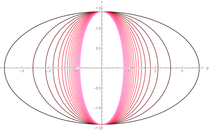
Figure 1: Set of trajectories of the regularized Kepler problem (Equation 77) with $g=1$ represented in the space $(Q,\mathcal{V})$ $Q$ being the modulus of the position and $\mathcal{V})$ the modulus of the velocity.

Notice also that a deformation of the type of a $f$–oscillator, and the resulting change in the tangent bundle structure of the system produces also a transformation at the level of the space of motions. Indeed, the change in the frequencies of the different orbits is a clear indication of a transformation in the parametrization of trajectories and hence in a mapping from one point in the space of motions of the undeformed system to another point of the deformed one. Our goal in the next section is to study whether a suitable deformation function $f$ may achieve to define invertible mappings between the spaces of motion of the deformed system and the space of motions of the regularized Kepler problem.

5.3 Application: finding a relation for a $f$–oscillator and the regularized Kepler problem

In the previous sections we have been able to identify mechanisms which allow us to construct alternative tangent bundle descriptions for the regularization of the dynamical vector fields corresponding to closed orbits of the Kepler problem and for the Lagrangian description of the $f$–oscillators. Furthermore, in both cases the resulting vector fields have the same formal expression and hence it is natural to study whether it is possible to relate both descriptions.

If we consider the $f$–oscillator defined on the same four dimensional configuration space as the regularized Kepler problem of Equation (77), both vector fields will produce trajectories of 4-dimensional harmonic oscillators with a given set of frequencies depending on the points of the carrier space. The submanifolds of points with the same frequencies will be different in one case and the other, but sharing the same frequency is sufficient to identify the corresponding motions of the two vector fields. Therefore, we must determine a function $f$ to produce a $f$–oscillator such that the vector field (82) takes a set of frequencies identical to those of the set orbits of the regularized Kepler problem which project on closed orbits of the three dimensional one. Thus the choice must satisfy

$$\Omega=f^{\prime}(|E|),$$ (84)

Since the frequencies associated to each $\Sigma(E)$ are equal to $\frac{\sqrt{2|E|^{3}}}{g}$ we have to choose a deformation function $f$ satisfying

$$f^{\prime}(|E|)=\frac{\sqrt{2|E|^{3}}}{g}\Rightarrow f(|E|)=\frac{1}{10g}(2|E|)^{5/2}+C.$$ (85)

The constant can safely be fixed to zero.

If we consider the set of motions of the corresponding $f$–oscillator we would get the set plotted in Figure 2. Clearly there exists a one-to-one correspondence between this space of motions and that of Figure 1, since the function $f$ has been chosen to produce the same frequency for the periodic motion.

Figure 2: Set of trajectories of the $f$–oscillator (Equation 82) with function equal to Equation (85) represented in the space $(Q,\mathcal{V})$ $Q$ being the modulus of the position and $\mathcal{V})$ the modulus of the velocity.

With respect to such a system, the trajectory of the Kepler orbit with energy $E$ can be obtained by factorization of the $f$–oscillator orbit and the correspondence between both orbit sets $\Psi$, i.e.

$$\Phi_{t}^{K}=\Psi\circ\Phi_{t}^{f},$$ (86)

where we represent by $\Phi_{t}^{K}$ and $\Phi_{t}^{f}$ the flows of the corresponding systems at time $t$. As both vector fields are complete, Equation (86) can be used to identify the corresponding spaces of motion in a trivial way.

But it is also important to remark the importance of the changes in the tangent bundle structures of both systems: without them it would not have been possible to define the mapping above in a simple way.

6 Conclusions

In this paper we have seen how the choice among alternative tangent bundle structures for the carrier space $M$ of a certain dynamical vector field $\Gamma$ can provide us with useful tools to describe interesting properties of the corresponding dynamics. We have been able to identify general properties to identify the base manifold by providing a set of coordinate functions $\{Q^{i}\}$ and the corresponding submanifold $Q$ parametrized by them:

• $Q$ must have half the dimension of the carrier space

• the functions must be functionally independent

• $Q$ must contain no fixed points of $\Gamma$

• the level set of all the coordinate functions (i.e., a point $p\in Q$) must define a submanifold of $M$ which is a vector space (the corresponding tangent space at the point of the base defined by $Q^{i}=p^{i}$)

• the set of velocity coordinates

  $$\mathcal{V}^{k}=\mathcal{L}_{\Gamma}Q^{k},$$

  must be functionally independent among them and with respect to the coordinate functions.

In these circumstances, we can define a tangent bundle structure that makes $\Gamma$ a SODE. In particular, we have seen in Section 4.3 how common tools as the reparametrization of vector fields can be made compatible with a redefinition of the bundle structure which makes the reparametrized vector field a SODE. A particular example of this construction is provided in Section 4.4 by the reparametrized Kepler problem in four dimensions. A similar property has been proved for $f$–oscillators in Section 4.5: the deformation by constants of the motion can preserve the SODE property by a suitable redefinition of the tangent bundle structure given by Equation (78) and Equation (79). The usefulness of these alternative bundle structures can be seen in the last section: in some particular cases, it is possible to use the resulting tangent bundle structures to define mappings between the spaces of motions of two different systems, which may remain hidden without them. In particular we have been able to construct a one-to-one mapping between the spaces of motion of the regularized Kepler problem and of a suitable $f$-oscillator. Such a mapping circumvents, partially, the obstruction defined by the energy-period theorem which prevents the existence of a diffeomorphism between two systems having closed orbits with different periods, as it happens with the Kepler problem and the harmonic oscillator.

In the quantum domain it is possible to consider an analogue construction by the redefinition of the hermitian product of the Hilbert space. Indeed, in Quantum Mechanics it is possible to consider alternative Hilbert space structures for the space of states and with respect to them self-adjointness of operators may be adapted to different situations (see, for instance, [8] for an analysis of hydrogen atom). In that case we may also search for relations between different models with deformed oscillators, where the deformation function may allow to match the equispaced spectrum of the harmonic oscillator with the spectrum of the other model (for instance the hydrogen atom). This is ongoing research that we expect to publish soon.

References

- [1] J. F. Cariñena, A. Ibort, G. Marmo, and G. Morandi. Geometry from Dynamics, Classical and Quantum. Springer, 2014.
- [2] J.F. Cariñena, J. Clemente-Gallardo, and Giuseppe Marmo. Reduction procedures in classical and quantum mechanics. International Journal of Geometric Methods in Modern Physics, 4(8):1363–1403, 2007.
- [3] M Crampin. Defining Euler-Lagrange fields in terms of almost tangent structures. Physics Letters A, 95(9):466–468, 1983.
- [4] M Crampin. Tangent bundle geometry for Lagrangian dynamics. Journal of Physics A: Mathematical and General, 16:3755–3772, 1983.
- [5] M. Crampin and G. Thompson. Affine bundles and integrable almost tangent structures. Mathematical Proceedings of the Cambridge Philosophical Society, 98(01):61–71, 1985.
- [6] RH Cushman and JJ Duistermaat. A characterization of the Ligon-Schaaf regularization map. Comm. Pure Appl. Math., 50(8):773–787, 1997.
- [7] A. D’Avanzo and G. Marmo. Reduction and unfolding: the Kepler problem. Int. J. Geom. Meth. Mod. Phys., 2:83–109, 2005.
- [8] A. D’Avanzo, G. Marmo, and A. Valentino. Reduction and Unfolding for Quantum Systems: the Hydrogen Atom. Int. J. Geom. Meth. Mod. Phys., 2:1043–1062, 2005.
- [9] S. De Filippo, G. Landi, G. Marmo, and G. Vilasi. Tensor fields defining a tangent bundle structure. Ann. de l’I.H.P., Section A, 50(2):205–218, 1989.
- [10] W. B. Gordon. On the relation between period and energy in periodic dynamical systems. J. Math. Mech, 19:111–114, 1969.
- [11] W. B. Gordon. Conservative dynamical systems involving strong forces. Transactions of the American Mathematical Society, 204:113–135, 1975.
- [12] Joseph Grifone. Structure presque-tangente et connexions I. Université de Grenoble. Annales de l’Institut Fourier, 22(1):287–334, 1972.
- [13] Joseph Grifone. Structure presque-tangente et connexions II. Universit{é} de Grenoble. Annales de l’Institut Fourier, 22(3):291–338, 1972.
- [14] G. Györgyi. Kepler’s Equation, Fock Variables, Bacry’s Generators and Dirac Brackets. Il Nuovo Cimento A Series 10, 53(3):717–736, 1968.
- [15] H. Hopf. Über die Abbildungen der dreidimensionalen Sphäre auf die Kugelfläche. Math. Annalen, 104:637–665, 1931.
- [16] P Kustaanheimo and E Stiefel. Perturbation theory of Kepler motion based on spinor regularization. Journal für Mathematik. Bd, 218:204–219, 1965.
- [17] D. C. Lewis. Families of Periodic Solutions of Systems having Relatively Invariant Line Integrals. Proceedings of the American Mathematical Society, 6(2):181–185, 1955.
- [18] T. Ligon and M. Schaaf. On the global symmetry of the classical Kepler problem. Reports on Mathematical Physics, 9(3):281–300, 1976.
- [19] V. I. Man’ko, G. Marmo, E. C. G. Sudarshan, and F. Zaccaria. f-Oscillators and Nonlinear Coherent States. Physica Scripta, 55(5):528–541, 1997.
- [20] Ch. M. Marle. A property of conformally Hamiltonian vector fields; Application to the Kepler problem. The Journal of Geometric Mechanics, 4(2):181–206, 2012.
- [21] G. Marmo and A. Simoni. Q-dynamical systems and constants of motion. Lettere Al Nuovo Cimento Series 2, 15(6):179–184, 1976.
- [22] R. Palais. A global formulation of the Lie theory of transformation groups. Memoirs of the AMS, 22, 1957.
- [23] J M Souriau. Structure of Dynamical Systems, Birkhuser, Boston, 1997.
- [24] H.K. Urbantke. The Hopf fibration—seven times in physics. Journal of Geometry and Physics, 46(2):125–150, 2003.
- [25] N.M.J. Woodhouse. Geometric quantization. Oxford University Press, 2nd edition, 1997.
- [26] Chengjun Zhu and J. R. Klauder. Classical symptoms of quantum illnesses. American Journal of Physics, 61(7):605, 1993.