Analysis of $P_{c}^{+}(4380)$ and $P_{c}^{+}(4450)$ as pentaquark states in the molecular picture with QCD sum rules

Abstract

To better understand the nature and internal structure of the exotic states discovered by many collaborations, more information on their electromagnetic properties and their strong and weak interactions with other hadrons is needed. The residue or current coupling constant of these states together with their mass are the main inputs in determinations of such properties. We perform QCD sum rules analyses on the hidden-charm pentaquark states with spin-parities $J^{P}=\frac{3}{2}^{\pm}$ and $J^{P}=\frac{5}{2}^{\pm}$ to calculate their residue and mass. In the calculations, we adopt a molecular picture for $J^{P}=\frac{3}{2}^{\pm}$ states and a mixed current in a molecular form for $J^{P}=\frac{5}{2}^{\pm}$. Our analyses show that the $P_{c}^{+}(4380)$ and $P_{c}^{+}(4450)$, observed by LHCb Collaboration, can be considered as hidden-charm pentaquark states with $J^{P}=\frac{3}{2}^{-}$ and $J^{P}=\frac{5}{2}^{+}$, respectively.

I Introduction

The recent experimental progresses resulted in the observation of exotic hadrons have placed this subject at the focus of interest. These hadrons have an internal structure that is more complex than those containing usual $q\bar{q}$ or $qqq$ quark contents. The existence of these types of hadrons is forbidden neither in the naive quark model that provides good description for the observed conventional hadrons nor in quantum chromodynamics (QCD), which describes the interactions among quarks and gluons. Starting from the observation of $X(3872)$ in 2003 by Belle collaboration Belle many experiments have been designed to identify and measure the parameters of the non-conventional particles especially, the XYZ states. These experimental attempts have been accompanied by a lot of theoretical works on tetraquarks, pentaquarks, hybrids, glueballs, etc.

The first detailed theoretical analysis on the exotic states provided by Jaffe Jaffe was followed by a vast amount of theoretical studies that investigated the properties of these particles. Among these states are the pentaquarks for which the first claim of observation was in 2003 through the interaction $\gamma n\rightarrow nK^{+}K^{-}$ Nakano suggesting a possible quark content $uudd\bar{s}$ ($\Theta^{+}$) with strangeness $S=+1$. Even before this claim, there have been several works on the properties of pentaquarks (see for instance Ref. Gignoux ; Hogaasen ; Strottman ; Lipkin1 ; Fleck ; Oh ; Chow ; Shmatikov ; Genovese ; Lipkin2 ; Lichtenberg ). Later, two other experiments also found some positive signatures Barmin:2003vv ; Stepanyan:2003qr . With the motivation provided by those results, there came another estimation on the anti-charmed analogue of $\Theta^{+}$ having quark content $uudd\bar{c}$ called as $\Theta_{c}$. Its mass together with the mass of its b-partner $\Theta_{b}$ were predicted as $2985\pm 50$ MeV and $6398\pm 50$ MeV, respectively Karliner:2003si . The masses of $\Theta^{+}$, $\Theta_{c}$ and $\Theta_{b}$ states were also predicted in Ref. Cheung:2003de . The masses and other properties of $\Theta^{+}$, $\Theta_{c}$ and $\Theta_{b}$ were then extensively examined via various methods (see for instance Refs. Matheus:2003xr ; Csikor:2003ng ; Oh:2003kw ; Gerasyuta:2003qg ; Bijker:2003pm ; Zhao:2003gs ; Huang:2003bu ; Nakayama:2003by ; Liu:2003ab ; Ko:2003xx ; Huang:2004tn ; Lee:2004bsa ; Kim:2004fka ; Karliner:2003dt ; Chiu:2004gg ; Bijker:2004gr ; He:2004nz ; Eidemuller:2004ra ; Kim:2004pu ; Melikhov:2004qh ; Bicudo ; Mathur:2004jr ; Lee:2004xk ; Nishikawa:2004tk ; Kim:2005yi ; Wang:2005jea ; Wang:2005gv ; Eidemuller:2005jm ; Wang:2005ms ; Lee:2005ny ; Panda:2005mj ; Sarac:2005fn and references therein). In the mean time, the observation of the $\Theta_{c}$ was announced later by H1 collaboration at HERA Aktas:2004qf . However, besides all these experiments having positive results and related theoretical studies, some experiments announced negative signals on the existence of those particles Bai:2004gk ; Knopfle:2004tu ; Pinkenburg:2004ux ; Harris:2004kx ; Karshon:2004tf ; Abt:2004tz ; Aubert:2004bm ; Litvintsev:2004yw ; Karshon:2004kt ; Link:2005ti ; Aubert:2007qea . All these controversial results have made the subject more intriguing from theoretical point of view since theoretical works might provide valuable insights into the experimental searches.

All those labor in the searches of exotic states finally resulted in success in experimental side. With the report of observation of $Z_{c}$ Ablikim:2013mio in 2013, which might be an indication of the existence of pentaquark states, the pentaquark captured the attentions once more. However some experimental searches on pentaquarks still came into view with null results such as the result of ALICE Collaboration investigating $\phi(1869)$ pentaquark Abelev:2014qqa and J-PARC E19 Collaboration searching for $\Theta^{+}$ Moritsu::2014qra state. On the other hand the theoretical studies indicated that the search on the pentaquark containing heavy quark constituents is still necessary Gerasyuta:2014wka due to the effect of such a structure on the stability of the hadronic structures beyond the traditional hadrons Li:2014gra . In 2015 the observation of two pentaquark states, $P_{c}^{+}(4380)$ and $P_{c}^{+}(4450)$, was finally reported by LHCb Collaboration in the $\Lambda_{b}^{0}\rightarrow J/\psi K^{-}p$ decays. The reported masses were $4380\pm 8\pm 29$ MeV and $4449.8\pm 1.7\pm 2.5$ MeV with corresponding spins $3/2$ and $5/2$ and decay widths $205\pm 18\pm 86$ MeV and $39\pm 5\pm 19$ MeV, respectively Aaij:2015tga .

The observation of LHCb put these particles at the focus of intense theoretical works which aimed to explain the properties of these states. To give an explanation on their substructure different models were proposed. Their nature was examined using meson baryon molecular model Roca:2015dva ; Chen:2015loa ; Huang:2015uda ; Meissner:2015mza ; Xiao:2015fia ; He:2015cea ; Chen:2015moa ; Chen:2016heh ; Yamaguchi:2016ote ; Wang:2016dzu , diquark-triquark model Wang:2016dzu ; Zhu:2015bba ; Lebed:2015tna , diquark-diquark-antiquark model Wang:2016dzu ; Anisovich:2015cia ; Maiani:2015vwa ; Ghosh:2015ksa ; Wang:2015ava ; Wang:2015epa ; Wang:2015ixb and topological soliton model Scoccola:2015nia . They were also investigated taking into account the possibility of their being a kinematical effect or a real resonance state considering the triangle singularity mechanism Guo:2015umn ; Mikhasenko:2015vca ; Liu:2015fea . In oset , however, it is concluded that with the presently claimed experimental quantum numbers, the triangle singularity cannot be the answer for the peaks. One can find a review on the multiquark states including pentaquarks in Ref. Chen:2016qju .

All these developments make it necessary to study pentaquarks more deeply to gain information on their nature and substructure. The theoretical investigations on their spectroscopic and electromagnetic properties together with their strong and weak decays may provide valuable insights for the future experimental searches. Moreover the comparison between new theoretical findings and existing experimental and theoretical results may lead to a better understanding on the nature of these particles as well as dynamics of the strong interaction. With this motivation, in this paper, we investigate the residue and mass of the hidden-charm pentaquark states with the spin-parities $J^{P}=\frac{3}{2}^{\pm}$ and $J^{P}=\frac{5}{2}^{\pm}$. To fulfill this aim we apply QCD sum rule method Shifman:1978bx ; Shifman:1978by via a choice of interpolating current in the molecular form. Here we shall remark that the QCD sum rule approach in its standard form was formulated to reproduce the mass of the lowest hadronic state in a given channel with assuming that there are no other resonances close to the lowest one. We apply this method to reproduce the experimental data in the channels under consideration with the assumption that there are no other prominent resonances close to the lowest states with $J=\frac{3}{2}$ and $J=\frac{5}{2}$. In principle, there can be many interpolating currents with the same quantum numbers and flavor contents to investigate the states under consideration and there are no preferable interpolating currents. We choose a molecular picture and investigate these states by considering their interpolating currents in the anti-charmed meson-charmed baryon form. For the states with $J=\frac{5}{2}$ we consider an admixture of $[\bar{D}\Sigma_{c}^{*}]$ and $[\bar{D}^{*}\Lambda_{c}]$ and use a mixed anti-charmed meson-charmed baryon molecular current. In choosing this current we consider the discussion given in Ref. Chen:2016otp which states that a choice of mixed molecular current provides a mass result consistent with the experimental data. For $J=\frac{3}{2}$ states we also use an anti-charmed meson-charmed baryon molecular current, namely $\bar{D}^{*}\Sigma_{c}$. As the residue is the main input in the analysis of the width, electromagnetic properties as well as the strong and weak decays of these particles, the main goal in this work is to calculate the residue of these pentaquarks with both parities considering the molecular and mixed molecular currents for $J=\frac{3}{2}$ and $J=\frac{5}{2}$ states, respectively. We also calculate the mass of these states in the same pictures. Here we shall remark that in Refs. Wang:2015epa ; Chen:2015moa the authors use the QCD sum rule method to investigate these pentaquark states, as well. In Ref. Chen:2015moa the authors calculate only the masses of the $J^{P}=\frac{3}{2}^{-}$ and $J^{P}=\frac{5}{2}^{+}$ pentaquark states with the same currents and internal quark organizations as the present work. In Ref. Wang:2015epa , however, the author applies diquark-diquark-antiquark type interpolating currents to calculate the mass and residue of the $J^{P}=\frac{3}{2}^{-}$ and $J^{P}=\frac{5}{2}^{+}$ pentaquark states.

The present work has the following outline. In Sections II and III the details of the mass and residue calculations for the hidden-charm pentaquark states with $J=\frac{3}{2}$ and $J=\frac{5}{2}$ are presented, respectively. Section IV is set apart to the numerical analysis and discussion of the results. Last section is devoted to the summary and outlook.

II The hidden-charm pentaquark states with $J=\frac{3}{2}$

This section is devoted to present the details of the calculations on mass and residue of the pentaquark states with $\frac{3}{2}$ and both the positive and negative parities. The starting point is to consider the following two point correlation function:

$$\Pi_{1\mu\nu}(p)=i\int d^{4}xe^{ip\cdot x}\langle 0|\mathcal{T}\{J_{\mu}^{\bar{D}^{*}\Sigma_{c}}(x)\bar{J}_{\nu}^{\bar{D}^{*}\Sigma_{c}}(0)\}|0\rangle,$$ (1)

where $J_{\mu}^{\bar{D}^{*}\Sigma_{c}}(x)$ is the interpolating current with $J^{P}=\frac{3}{2}^{-}$ that couples to both the negative and positive parity particles Chen:2015moa :

$$J_{\mu}^{\bar{D}^{*}\Sigma_{c}}=[\bar{c}_{d}\gamma_{\mu}d_{d}][\epsilon_{abc}(u_{a}^{T}C\gamma_{\theta}u_{b})\gamma^{\theta}\gamma_{5}c_{c}].$$ (2)

The first step is to calculate the correlation function in terms of hadronic degrees of freedom containing the physical parameters of the states under consideration. This requires the insertion of a complete set of the hadronic states into Eq. (1) that is followed by an integration over $x$. This leads to

$$\Pi_{1\mu\nu}^{\mathrm{Phys}}(p) = \frac{\langle 0|J_{\mu}|\frac{3}{2}^{+}(p)\rangle\langle\frac{3}{2}^{+}(p)|\bar{J}_{\nu}|0\rangle}{m_{+}^{2}-p^{2}}$$ (3)

$$+ \frac{\langle 0|J_{\mu}|\frac{3}{2}^{-}(p)\rangle\langle\frac{3}{2}^{-}(p)|\bar{J}_{\nu}|0\rangle}{m_{-}^{2}-p^{2}}+\textellipsis\ ,$$

where $m_{\pm}$ are the masses of the positive and negative parity particles. The dots appearing in the last equation represent the contributions coming from the higher states and continuum resonances. The matrix elements in Eq. (3) are parameterized in terms of the residues $\lambda_{+}$ and $\lambda_{-}$ as well as the corresponding spinors as

$$\langle 0|J_{\mu}|\frac{3}{2}^{+}(p)\rangle = \lambda_{+}\gamma_{5}u_{\mu}(p),$$

$$\langle 0|J_{\mu}|\frac{3}{2}^{-}(p)\rangle = \lambda_{-}u_{\mu}(p),$$ (4)

where the negative parity nature of the current under consideration has been imposed. Here we should remark that the $J_{\mu}$ current couples not only to the spin-3/2 states, but also to the spin-1/2 states with both parities. We will choose appropriate structures to take into account only the particles with spin-3/2. The summation over the Rarita-Schwinger spinor is applied in the form

$$\sum_{s}u_{\mu}(p,s)\bar{u}_{\nu}(p,s) = -({\not{p}}+m)\left[g_{\mu\nu}-\frac{1}{3}\gamma_{\mu}\gamma_{\nu}\right.$$ (5)

$$- \left.\frac{2p_{\mu}p_{\nu}}{3m^{2}}+\frac{p_{\mu}\gamma_{\nu}-p_{\nu}\gamma_{\mu}}{3m}\right].$$

After the application of Borel transformation, the hadronic side gets its final form in terms of different structures,

$$\mathcal{B}_{p^{2}}\Pi_{1\mu\nu}^{\mathrm{Phys}}(p)=-\lambda_{+}^{2}e^{-\frac{m_{+}^{2}}{M^{2}}}(-\gamma_{5})({\not{p}}+m_{+})$$

$$\times \left[g_{\mu\nu}-\frac{1}{3}\gamma_{\mu}\gamma_{\nu}-\frac{2p_{\mu}p_{\nu}}{3m_{+}^{2}}+\frac{p_{\mu}\gamma_{\nu}-p_{\nu}\gamma_{\mu}}{3m_{+}}\right]\gamma_{5}$$

$$- \lambda_{-}^{2}e^{-\frac{m_{-}^{2}}{M^{2}}}({\not{p}}+m_{-})$$

$$\times \left[g_{\mu\nu}-\frac{1}{3}\gamma_{\mu}\gamma_{\nu}-\frac{2p_{\mu}p_{\nu}}{3m_{-}^{2}}+\frac{p_{\mu}\gamma_{\nu}-p_{\nu}\gamma_{\mu}}{3m_{-}}\right]+\textellipsis\ ,$$

where $M^{2}$ is the Borel parameter that should be fixed later. To avoid the unwanted contributions coming from the spin-1/2 states, we select the $g_{\mu\nu}$ and ${\not{p}}g_{\mu\nu}$ structures after ordering of the Dirac matrices.

To get the QCD sum rules one needs also to calculate the same correlation function in QCD side in terms of quark-gluon degrees of freedom in deep Euclidean region using the operator product expansion (OPE). This requires the contraction of the heavy and light quark fields which leads to the result

$$\Pi_{1\mu\nu}^{\mathrm{QCD}}(p)=-i\int d^{4}xe^{ip\cdot x}\epsilon^{abc}\epsilon^{a^{\prime}b^{\prime}c^{\prime}}$$

$$\mathrm{Tr}\left[\gamma_{\mu}S_{d}^{dd^{\prime}}(x)\gamma_{\nu}S_{c}^{d^{\prime}d}(-x)\right]\left(\gamma{\theta}\gamma_{5}S_{c}^{cc^{\prime}}(x)\gamma_{5}\gamma{\beta}\right)$$

$$\left\{\mathrm{Tr}\left[\gamma_{\beta}\widetilde{S}_{u}^{aa^{\prime}}(x)\gamma_{\theta}S_{u}^{bb^{\prime}}(x)\right]-\mathrm{Tr}\left[\gamma_{\beta}\widetilde{S}_{u}^{ba^{\prime}}(x)\gamma_{\theta}S_{u}^{ab^{\prime}}(x)\right]\right\},$$

(7)

where $\widetilde{S}_{u(d)}(x)=CS_{u(d)}^{T}(x)C$ and the $S_{u(d)}^{ab}(x)$ and $S_{c}^{ab}(x)$ appering in Eq. (7) are the propagators of the light $u(d)$ and heavy $c$ quarks, respectively. The explicit expression for light quark propagator has the following form:

$$S_{q}^{ab}(x)=i\delta_{ab}\frac{\not{x}}{2\pi^{2}x^{4}}-\delta_{ab}\frac{m_{q}}{4\pi^{2}x^{2}}-\delta_{ab}\frac{\langle\overline{q}q\rangle}{12}$$

$$+i\delta_{ab}\frac{\not{x}m_{q}\langle\overline{q}q\rangle}{48}-\delta_{ab}\frac{x^{2}}{192}\langle\overline{q}g_{s}\sigma Gq\rangle+i\delta_{ab}\frac{x^{2}\not{x}m_{q}}{1152}$$

$$\times\langle\overline{q}g_{s}\sigma Gq\rangle-i\frac{g_{s}G_{ab}^{\alpha\beta}}{32\pi^{2}x^{2}}\left[\not{x}{\sigma_{\alpha\beta}+\sigma_{\alpha\beta}}\not{x}\right]$$

$$-i\delta_{ab}\frac{x^{2}\not{x}g_{s}^{2}\langle\overline{q}q\rangle^{2}}{7776}+\textellipsis\ ,$$ (8)

and the heavy quark propagator is given as Reinders:1984sr

$$S_{c}^{ab}(x)=i\int\frac{d^{4}k}{(2\pi)^{4}}e^{-ikx}\Bigg{\{}\frac{\delta_{ab}\left({\not{k}}+m_{c}\right)}{k^{2}-m_{c}^{2}}$$

$$-\frac{g_{s}G_{ab}^{\alpha\beta}}{4}\frac{\sigma_{\alpha\beta}\left({\not{k}}+m_{c}\right)+\left({\not{k}}+m_{c}\right)\sigma_{\alpha\beta}}{(k^{2}-m_{c}^{2})^{2}}$$

$$+\frac{g_{s}^{2}G^{2}}{12}\delta_{ab}m_{c}\frac{k^{2}+m_{c}{\not{k}}}{(k^{2}-m_{c}^{2})^{4}}+\textellipsis\ \Bigg{\}},$$

where we used the short-hand notations

$$G_{ab}^{\alpha\beta}=G_{A}^{\alpha\beta}t_{ab}^{A},\,\,~{}~{}G^{2}=G_{\alpha\beta}^{A}G_{\alpha\beta}^{A},$$ (10)

in which $A=1,\,2,\,\textellipsis\ ,\,8$ and $a,\,b=1,2,3$ are color indices and $t^{A}=\lambda^{A}/2$, with $\lambda^{A}$ being the Gell-Mann matrices.

The calculations in OPE side proceed by writing the correlation function in a dispersion integral form,

$$\Pi_{1\mu\nu}^{\mathrm{QCD}}(p^{2})=\int_{(2m_{c})^{2}}^{s_{0}}\frac{\rho_{\frac{3}{2}}^{\mathrm{QCD}}(s)}{s-p^{2}}ds+\textellipsis\ ,$$ (11)

where $\rho_{\frac{3}{2}}^{\mathrm{QCD}}(s)$ is the two-point spectral density, which is found via the imaginary part of the correlation function following the standard procedures. Here $s_{0}$ is the continuum threshold. The calculations are very lengthy. For details we refer the interested reader to e.g. Refs. Azizi:2015jya ; Agaev:2016dev . The explicit expression of the spectral density $\rho_{\frac{3}{2}}^{\mathrm{QCD}}(s)$, for instance for $g_{\mu\nu}$ structure, is given in the Appendix. We apply the Borel transformation, with the aim of suppressing the contributions of the higher states and continuum, to this side also to find the correlation function in its final form in the Borel scheme.

Now, we match the coefficients of the structures $g_{\mu\nu}$ and ${\not{p}}g_{\mu\nu}$, from both the hadronic and OPE sides and apply a continuum subtraction supported by the quark-hadron duality assumption. This leads to the sum rules

$$m_{+}\lambda_{+}^{2}e^{-m_{+}^{2}/M^{2}}-m_{-}\lambda_{-}^{2}e^{-m_{-}^{2}/M^{2}}=\Pi^{1}_{1},$$ (12)

$$- \lambda_{+}^{2}e^{-m_{+}^{2}/M^{2}}-\lambda_{-}^{2}e^{-m_{-}^{2}/M^{2}}=\Pi^{2}_{1},$$

including the masses and residues of the $\frac{3}{2}^{+}$ and $\frac{3}{2}^{-}$ states. In the last equation $\Pi^{1}_{1}$ and $\Pi^{2}_{1}$ are the invariant functions obtained from the OPE side and correspond to the coefficients of the structures $g_{\mu\nu}$ and ${\not{p}}g_{\mu\nu}$, respectively.

Note that Eq. (12) contains two sum rules with four unknowns: two masses $m_{+}$ and $m_{-}$ as well as two residues $\lambda_{+}$ and $\lambda_{-}$. Hence, to find these four unknowns, we need two more equations, which are found by applying the derivatives with respect to $\frac{1}{M^{2}}$ to both sides of the above sum rules. By simultaneous solving of the four resulted equations one can find the four unknowns in terms of QCD degrees of freedom as well as the continuum threshold and Borel mass parameter.

III The hidden-charm pentaquark states with $J=\frac{5}{2}$

In this section we follow similar steps as the previous section. In this case the following two point correlation function is used:

$$\Pi_{2\mu\nu\rho\sigma}(p)=i\int d^{4}xe^{ip\cdot x}\langle 0|\mathcal{T}\{J_{\mu\nu}(x)\bar{J}_{\rho\sigma}(0)\}|0\rangle,$$ (13)

where $J_{\mu\nu}(x)$ is the interpolating current having quantum numbers $J^{P}=\frac{5}{2}^{+}$. This current is defined in terms of the mixed currents of $J_{\mu\nu}^{\bar{D}\Sigma_{c}^{*}}$ and $J_{\mu\nu}^{\bar{D}^{*}\Lambda_{c}}$ via the expression Chen:2015moa

$$J_{\mu\nu}(x)=\mathrm{\sin\theta}\times J_{\mu\nu}^{\bar{D}\Sigma_{c}^{*}}+\mathrm{\cos\theta}\times J_{\mu\nu}^{\bar{D}^{*}\Lambda_{c}},$$ (14)

where $\theta$ is a mixing angle and

$$J_{\mu\nu}^{\bar{D}\Sigma_{c}^{*}} = [\bar{c}_{d}\gamma_{\mu}\gamma_{5}d_{d}][\epsilon_{abc}(u_{a}^{T}C\gamma_{\nu}u_{b})c_{c}]+\{\mu\leftrightarrow\nu\},$$

$$J_{\mu\nu}^{\bar{D}^{*}\Lambda_{c}} = [\bar{c}_{d}\gamma_{\mu}u_{d}][\epsilon_{abc}(u_{a}^{T}C\gamma_{\nu}\gamma_{5}d_{b})c_{c}]+\{\mu\leftrightarrow\nu\}.$$

In Ref. Chen:2015moa it is found that the above current with the mixing angle $\theta=(-51\pm 5)^{\circ}$ gives a result consistent with the experimental mass of $P_{c}(4450)$ state .

The hadronic side after integration over $x$ is obtained as

$$\Pi_{2\mu\nu\rho\sigma}^{\mathrm{Phys}}(p) = \frac{\langle 0|J_{\mu\nu}|\frac{5}{2}^{+}(p)\rangle\langle\frac{5}{2}^{+}(p)|\bar{J}_{\rho\sigma}|0\rangle}{m_{+}^{2}-p^{2}}$$ (16)

$$+ \frac{\langle 0|J_{\mu\nu}|\frac{5}{2}^{-}(p)\rangle\langle\frac{5}{2}^{-}(p)|\bar{J}_{\rho\sigma}|0\rangle}{m_{-}^{2}-p^{2}}$$

$$+ \textellipsis\ ,$$

with $m_{\pm}$ being the masses of the $\frac{5}{2}$ states having positive and negative parities. The contributions of the higher and continuum states resonances to the correlation function are represented via the dots appearing in the last equation. For the matrix elements presented in Eq. (16) the following parameterizations in terms of the residues and spinors are used:

$$\langle 0|J_{\mu\nu}|\frac{5}{2}^{+}(p)\rangle = \lambda_{+}u_{\mu\nu}(p),$$

$$\langle 0|J_{\mu\nu}|\frac{5}{2}^{-}(p)\rangle = \lambda_{-}\gamma_{5}u_{\mu\nu}(p).$$ (17)

The current $J_{\mu\nu}(x)$ also couples to the states with spin 3/2 and 1/2 with both parities. Again, we will choose the structures that only give contributions to the spin 5/2 particles. With the usage of the summation Wang:2015epa ,

$$\sum_{s}u_{\mu\nu}\bar{u}_{\rho\sigma} = ({\not{p}}+m)\left\{\frac{\widetilde{g}_{\mu\rho}\widetilde{g}_{\nu\sigma}+\widetilde{g}_{\mu\sigma}\widetilde{g}_{\nu\rho}}{2}-\frac{\widetilde{g}_{\mu\nu}\widetilde{g}_{\rho\sigma}}{5}\right.$$

$$- \frac{1}{10}\left(\gamma_{\mu}\gamma_{\rho}+\frac{\gamma_{\mu}p_{\rho}-\gamma_{\rho}p_{\mu}}{\sqrt{p^{2}}}-\frac{p_{\mu}p_{\rho}}{p^{2}}\right)\widetilde{g}_{\nu\sigma}$$

$$- \frac{1}{10}\left(\gamma_{\nu}\gamma_{\rho}+\frac{\gamma_{\nu}p_{\rho}-\gamma_{\rho}p_{\nu}}{\sqrt{p^{2}}}-\frac{p_{\nu}p_{\rho}}{p^{2}}\right)\widetilde{g}_{\mu\sigma}$$

$$- \frac{1}{10}\left(\gamma_{\mu}\gamma_{\sigma}+\frac{\gamma_{\mu}p_{\sigma}-\gamma_{\sigma}p_{\mu}}{\sqrt{p^{2}}}-\frac{p_{\mu}p_{\sigma}}{p^{2}}\right)\widetilde{g}_{\nu\rho}$$

$$- \left.\frac{1}{10}\left(\gamma_{\nu}\gamma_{\sigma}+\frac{\gamma_{\nu}p_{\sigma}-\gamma_{\sigma}p_{\nu}}{\sqrt{p^{2}}}-\frac{p_{\nu}p_{\sigma}}{p^{2}}\right)\widetilde{g}_{\mu\rho}\right\},$$

where $\widetilde{g}_{\mu\nu}=g_{\mu\nu}-\frac{p_{\mu}p_{\nu}}{p^{2}}$, the correlation function gets the form

$$\Pi_{2\mu\nu\rho\sigma}^{\mathrm{Phys}}(p) = \frac{\lambda_{+}^{2}}{(m_{+}^{2}-p^{2})}(\not{p}+m_{+})\frac{g_{\mu\rho}g_{\nu\sigma}+g_{\mu\sigma}g_{\nu\rho}}{2}$$ (19)

$$+ \frac{\lambda_{-}^{2}}{(m_{-}^{2}-p^{2})}(\not{p}-m_{-})\frac{g_{\mu\rho}g_{\nu\sigma}+g_{\mu\sigma}g_{\nu\rho}}{2}$$

$$+ \textellipsis\ ,$$

in terms of $m_{+}$, $m_{-}$, $\lambda_{+}$ and $\lambda_{-}$. In the last result there are other Lorentz structures giving contributions to the correlation function, however those structures mainly include contributions also coming from other pentaquark states having spin-1/2 and spin-3/2. To exclude such type of contributions, in the remaining part of the calculations we use the presented structures to extract the mass and residue of the states under consideration. Therefore the dots in Eq. (19) represents both the contributions coming from other Lorentz structures that are not written explicitly here as well as the contributions of higher states and continuum. Application of Borel transformation to Eq. (19) results in

$$\mathcal{B}_{p^{2}}\Pi_{2\mu\nu\rho\sigma}^{\mathrm{Phys}}(p) = \lambda_{+}^{2}e^{-\frac{m_{+}^{2}}{M^{2}}}(\not{p}+m_{+})(\frac{g_{\mu\rho}g_{\nu\sigma}+g_{\mu\sigma}g_{\nu\rho}}{2})$$ (20)

$$+ \lambda_{-}^{2}e^{-\frac{m_{-}^{2}}{M^{2}}}(\not{p}-m_{-})(\frac{g_{\mu\rho}g_{\nu\sigma}+g_{\mu\sigma}g_{\nu\rho}}{2})$$

$$+ \textellipsis\ .$$

In order to obtain the QCD side of the correlation function, we contract the heavy and light quark fields using the Wick’s theorem, which leads to

$$\Pi_{2\mu\nu\rho\sigma}^{\mathrm{QCD}}(p)=i\int d^{4}xe^{ipx}\epsilon^{abc}\epsilon^{a^{\prime}b^{\prime}c^{\prime}}\left\{\mathrm{\sin^{2}\theta}~{}S_{c}^{cc^{\prime}}(x)\right.$$ (21)

$$\times \left.\{\mathrm{Tr}\left[\gamma_{\mu}\gamma_{5}S_{d}^{dd^{\prime}}(x)\gamma_{5}\gamma_{\rho}S_{c}^{d^{\prime}d}(-x)\right]\left(\mathrm{Tr}\left[\gamma_{\nu}S_{u}^{ba^{\prime}}(x)\gamma_{\sigma}\right.\right.\right.$$

$$\times \left.\left.\left.\widetilde{S}_{u}^{ab^{\prime}}(x)\right]-\mathrm{Tr}\left[\gamma_{\nu}S_{u}^{bb^{\prime}}(x)\gamma_{\sigma}\widetilde{S}_{u}^{aa^{\prime}}(x)\right]\right)\}+\mathrm{\cos^{2}\theta}\right.$$

$$\times \left.S_{c}^{cc^{\prime}}(x)\{\mathrm{Tr}\left[\gamma_{\mu}S_{u}^{da^{\prime}}(x)\gamma_{\sigma}\gamma_{5}\widetilde{S}_{d}^{bb^{\prime}}(x)\gamma_{5}\gamma_{\nu}S_{u}^{ad^{\prime}}(x)\gamma_{\rho}\right.\right.$$

$$\times \left.\left.\left.S_{c}^{d^{\prime}d}(-x)\right]-\mathrm{Tr}\left[\gamma_{\mu}S_{u}^{dd^{\prime}}(x)\gamma_{\rho}S_{c}^{d^{\prime}d}(-x)\right]\mathrm{Tr}\Big{[}\gamma_{\nu}\gamma_{5}\right.\right.$$

$$\times \left.\left.S_{d}^{bb^{\prime}}(x)\gamma_{5}\gamma_{\sigma}\widetilde{S}_{u}^{aa^{\prime}}(x)\right]\}+\mathrm{\sin\theta}~{}\mathrm{\cos\theta}~{}S_{c}^{cc^{\prime}}(x)\right.$$

$$\times \left.\{\mathrm{Tr}\left[\gamma_{\mu}\gamma_{5}S_{d}^{db^{\prime}}(x)\gamma_{5}\gamma_{\sigma}\widetilde{S}_{u}^{aa^{\prime}}(x)\gamma_{\nu}S_{u}^{bd^{\prime}}(x)\right.\right.$$

$$\times \left.\left.\gamma_{\rho}S_{c}^{d^{\prime}d}(-x)\right]-\mathrm{Tr}\left[\gamma_{\mu}\gamma_{5}S_{d}^{db^{\prime}}(x)\gamma_{5}\gamma_{\sigma}\widetilde{S}_{u}^{ba^{\prime}}(x)\gamma_{\nu}\right.\right.$$

$$\times \left.\left.S_{u}^{ad^{\prime}}(x)\gamma_{\rho}S_{c}^{d^{\prime}d}(-x)\right]+\mathrm{Tr}\left[\gamma_{\mu}S_{u}^{db^{\prime}}(x)\gamma_{\sigma}\widetilde{S}_{u}^{aa^{\prime}}(x)\right.\right.$$

$$\times \left.\left.\gamma_{\nu}\gamma_{5}S_{d}^{bd^{\prime}}(x)\gamma_{5}\gamma_{\rho}S_{c}^{d^{\prime}d}(-x)\right]-\mathrm{Tr}\left[\gamma_{\mu}S_{u}^{da^{\prime}}(x)\gamma_{\sigma}\right.\right.$$

$$\times \left.\left.\widetilde{S}_{u}^{ab^{\prime}}(x)\gamma_{\nu}\gamma_{5}S_{d}^{bd^{\prime}}(x)\gamma_{5}\gamma_{\rho}S_{c}^{d^{\prime}d}(-x)\right]\}+\left(\mu\leftrightarrow\nu\right)\right.$$

$$+ \left.\left(\rho\leftrightarrow\sigma\right)+\left(\mu\leftrightarrow\nu,\rho\leftrightarrow\sigma\right)\right.\Big{\}}.$$

In this step we use the expressions of the heavy and light propagators and transform the calculations to the momentum space. By using the dispersion relation we find the imaginary part of the correlation function to extract the corresponding spectral density of $\frac{5}{2}$ state. Omitting the details of very lengthy calculations, we show the spectral density $\rho_{\frac{5}{2}}^{\mathrm{QCD}}(s)$ defining the state under consideration, for instance for $\frac{g_{\mu\rho}g_{\nu\sigma}+g_{\mu\sigma}g_{\nu\rho}}{2}$ structure, in the Appendix.

By matching the coefficients of the selected structures from both sides we find the sum rules

$$m_{+}\lambda_{+}^{2}e^{-m_{+}^{2}/M^{2}}-m_{-}\lambda_{-}^{2}e^{-m_{-}^{2}/M^{2}}=\Pi^{1}_{2},$$

$$\lambda_{+}^{2}e^{-m_{+}^{2}/M^{2}}+\lambda_{-}^{2}e^{-m_{-}^{2}/M^{2}}=\Pi^{2}_{2},$$ (22)

where $\Pi^{1}_{2}$ and $\Pi^{2}_{2}$ correspond to the coefficients of the structures $\frac{g_{\mu\rho}g_{\nu\sigma}+g_{\mu\sigma}g_{\nu\rho}}{2}$ and $\not{p}\frac{g_{\mu\rho}g_{\nu\sigma}+g_{\mu\sigma}g_{\nu\rho}}{2}$ in the OPE side, respectively. The four unknowns $m_{+}$ and $m_{-}$, $\lambda_{+}$ and $\lambda_{-}$ can be obtained using the above two sum rules and two extra sum rules obtained via applying the derivatives with respect to $\frac{1}{M^{2}}$ to their both sides.

IV Numerical results

Parameters	Values
$m_{c}$	$(1.27\pm 0.03)~{}\mathrm{GeV}$
$\langle\bar{q}q\rangle$	$(-0.24\pm 0.01)^{3}$ $\mathrm{GeV}^{3}$
$m_{0}^{2}$	$(0.8\pm 0.1)$ $\mathrm{GeV}^{2}$
$\langle\overline{q}g_{s}\sigma Gq\rangle$	$m_{0}^{2}\langle\bar{q}q\rangle$
$\langle\frac{\alpha_{s}G^{2}}{\pi}\rangle$	$(0.012\pm 0.004)$ $~{}\mathrm{GeV}^{4}$

Table 1: Some input parameters used in the calculations.

The QCD sum rules for the physical quantities under consideration contain some parameters such as quark, gluon and mixed condensates and mass of the $c$ quark. We collect their values in Table 1. We set the light quark masses, $m_{u}$ and $m_{d}$ to zero. In addition to the above parameters, there are two auxiliary parameters that should be fixed before going further, namely the continuum threshold $s_{0}$ and Borel parameter $M^{2}$. We find their working windows such that the physical quantities under consideration be roughly independent of these parameters. To determine the working interval of the Borel parameter one needs to consider two criteria: convergence of the series of OPE and adequate suppression of the higher states and continuum . Consideration of these criteria in the analysis leads to the intervals

$$4\ \mathrm{GeV}^{2}\leq M^{2}\leq 7\ \mathrm{GeV}^{2}.$$ (23)

To determine the working regions of the continuum threshold, we impose the conditions of pole dominance and OPE convergence. This leads to the interval

$$22\,\,\mathrm{GeV}^{2}\leq s_{0}\leq 24\,\,\mathrm{GeV}^{2},$$ (24)

for $\frac{3}{2}$ states with both parities and

$$22.5\,\,\mathrm{GeV}^{2}\leq s_{0}\leq 24.5\,\,\mathrm{GeV}^{2},$$ (25)

for $\frac{5}{2}$ states with negative and positive parities.

As examples, the variations of the mass and residue of the hidden-charm pentaquark with $J=\frac{5}{2}$ and positive parity with respect to the Borel parameter (continuum threshold) at different fixed values of the continuum threshold (Borel parameter) are depicted in figures 1 - 2. From these figures we see that the corresponding mass and residue demonstrate overall weak dependence on the variations of the Borel mass parameter and continuum threshold in their working intervals.

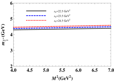
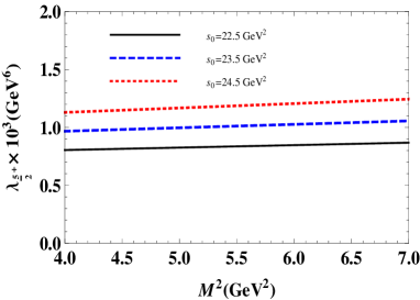
Figure 1: Left: The mass of the pentaquark with $J^{P}=\frac{5}{2}^{+}$ as a function of Borel parameter $M^{2}$ at different fixed values of the continuum threshold. Right: The residue of the pentaquark with $J^{P}=\frac{5}{2}^{+}$ as a function of Borel parameter $M^{2}$ at different fixed values of the continuum threshold.

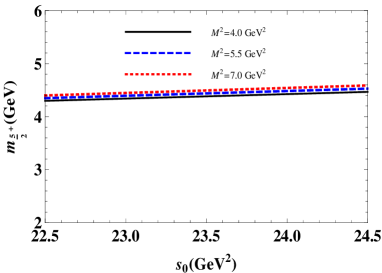
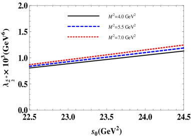
Figure 2: Left: The mass of the pentaquark with $J^{P}=\frac{5}{2}^{+}$ as a function of $s_{0}$ at different fixed values of the Borel parameter. Right: The residue of the pentaquark with $J^{P}=\frac{5}{2}^{+}$ as a function of $s_{0}$ at different fixed values of the Borel parameter.

Having determined the suitable intervals for the parameters $s_{0}$ and $M^{2}$ the next stage is to use them in the determination of mass and residue of the considered pentaquarks. The average values obtained from our calculations are presented in Table 2.

$J^{P}$	$m~{}(\mathrm{GeV})$	$\lambda~{}(\mathrm{GeV}^{6})$
$\frac{3}{2}^{+}$	$4.24\pm 0.16$	$(0.59\pm 0.07)\times 10^{-3}$
$\frac{3}{2}^{-}$	$4.30\pm 0.10$	$(0.94\pm 0.05)\times 10^{-3}$
$\frac{5}{2}^{+}$	$4.44\pm 0.15$	$(1.01\pm 0.23)\times 10^{-3}$
$\frac{5}{2}^{-}$	$4.20\pm 0.15$	$(0.51\pm 0.09)\times 10^{-3}$

Table 2: The results of QCD sum rules calculations for the mass and residue of the pentaquark states.

The errors in the given results arise due to the input parameters and also due to the uncertainties coming from the determination of the working windows of the auxiliary parameters $s_{0}$ and $M^{2}$. Comparison of the results on the masses with the experimental data of LHCb Collaboration, i.e., $m_{P_{c}^{+}(4380)}=4380\pm 8\pm 29$ MeV and $m_{P_{c}^{+}(4450)}=4449.8\pm 1.7\pm 2.5$ MeV Aaij:2015tga reveals that the $\frac{3}{2}^{-}$ state can be assigned to $P_{c}^{+}(4380)$ observed by LHCb. Our prediction for the mass of $\frac{5}{2}^{+}$ state is also consistent with the experimental data on the mass of the $P_{c}^{+}(4450)$. Our results on the masses of the $\frac{3}{2}^{-}$ and $\frac{5}{2}^{+}$ are also in a good agreement with the results of the theoretical works Wang:2015epa ; Chen:2015moa . Our predictions on the residues of the $\frac{3}{2}^{-}$ and $\frac{5}{2}^{+}$ states, within the errors, are also comparable with the predictions of Wang:2015epa , which applies diquark-diquark-antiquark type interpolating currents to calculate the mass and residue of the pentaquark states with $J^{P}=\frac{3}{2}^{-}$ and $J^{P}=\frac{5}{2}^{+}$. Here we note that using the experimental data for the mass of $\frac{3}{2}^{-}$ and $\frac{5}{2}^{+}$ states in our sum rules we find the residues $\lambda_{\frac{3}{2}^{-}}=(0.98\pm 0.05)\times 10^{-3}~{}\mathrm{GeV}^{6}$ and $\lambda_{\frac{5}{2}^{+}}=(1.02\pm 0.23)\times 10^{-3}~{}\mathrm{GeV}^{6}$, which are very close to the related values in the table 2 and we do not see considerable differences. Our results on the masses of the opposite-parity states, i.e., $\frac{3}{2}^{+}$ and $\frac{5}{2}^{-}$ as well as our predictions on the residues may be verified via different approaches.

V Summary and Outlook

We performed QCD sum rules analyses to compute the mass and residue of the hidden-charm pentaquark states with $J=\frac{3}{2}$ and $J=\frac{5}{2}$ and both the positive and negative parities. We adopted interpolating currents in an anti-charmed meson-charmed baryon molecular form of $\bar{D}^{*}\Sigma_{c}$ for states having $J=\frac{3}{2}$ and a mixed anti-charmed meson-charmed baryon molecular current of $[\bar{D}\Sigma_{c}^{*}]$ and $[\bar{D}^{*}\Lambda_{c}]$ for the states with $J=\frac{5}{2}$. By fixing the auxiliary parameters entered the calculations we obtained the values of the masses and residues for all the considered states. Our predictions on the mass of the $J^{P}=\frac{3}{2}^{-}$ and $J^{P}=\frac{5}{2}^{+}$ states are consistent with the experimental data of the LHCb collaboration for the masses of $P_{c}^{+}(4380)$ and $P_{c}^{+}(4450)$ states, respectively. Our results are also consistent with the predictions of the theoretical works Wang:2015epa ; Chen:2015moa on the masses. As we previously said Ref. Chen:2015moa uses the same picture and method with the present work but has prediction only for the masses of the $J^{P}=\frac{3}{2}^{-}$ and $J^{P}=\frac{5}{2}^{+}$ states. However, Ref. Wang:2015epa applies a different quark organization to predict also the masses of the $J^{P}=\frac{3}{2}^{-}$ and $J^{P}=\frac{5}{2}^{+}$ states.

By the adopted currents in the present study, we also derived the values of the residues for the considered states with both parities. We got comparable results on the residues of $J^{P}=\frac{3}{2}^{-}$ and $J^{P}=\frac{5}{2}^{+}$ states with those of Ref. Wang:2015epa within the errors. The residues can be used as the main inputs in the analyses of the electromagnetic properties and strong decays of the pentaquark states $P_{c}^{+}(4380)$ and $P_{c}^{+}(4450)$. Such analyses are needed and would be very important in determination of the internal structures, geometric shapes, charge distribution, multipole moments of these states and strong interactions inside them. In our future works we aim to analyze the strong, electromagnetic and weak decay channels of the pentaquark states considered in the present study to calculate the corresponding strong coupling constants as well as the widths of these states. Comparison of the theoretical results on many parameters of the pentaquarks with the present and future experimental data would help us better understand their quark organizations and will provide us with useful knowledge on the quantum chromodynamics of the exotic baryons.

Appendix A The two-point spectral densities

In this appendix we present the results for the two-point spectral densities obtained from QCD sum rules calculations. As examples, we only present those spectral densities corresponding to the structures $g_{\mu\nu}$ and $\frac{g_{\mu\rho}g_{\nu\sigma}+g_{\mu\sigma}g_{\nu\rho}}{2}$ for the states with $J=\frac{3}{2}$ and $J=\frac{5}{2}$, respectively. They are obtained as

$$\rho_{i}^{\mathrm{QCD}}(s)=\rho_{i}^{\mathrm{pert.}}(s)+\sum_{k=3}^{6}\rho_{i,k}(s),$$ (A.26)

with $i$ being $\frac{3}{2},\frac{5}{2}$. In Eq. (A.26) by $\rho_{i,k}(s)$ we denote the nonperturbative contributions to spectral densities $\rho_{i}^{\mathrm{QCD}}(s)$. The explicit expressions for $\rho_{i}^{\mathrm{pert}}(s)$ and $\rho_{i,k}(s)$ are obtained in terms of the integrals of the Feynman parameters $x$ and $y$ as:

$$\rho_{\frac{3}{2}}^{\mathrm{pert}}(s) = \frac{m_{c}}{5\times 2^{15}\pi^{8}}\int\limits_{0}^{1}dx\int\limits_{0}^{1-x}dy\frac{\left(6hsxy-m_{c}^{2}r\right)\left(hsxy-m_{c}^{2}r\right)^{4}}{h^{3}t^{8}}\Theta\left[L\right],$$

$$\rho_{\frac{3}{2},\mathrm{3}}(s) = \frac{m_{c}^{2}}{2^{9}\pi^{6}}\langle\bar{d}d\rangle\int\limits_{0}^{1}dx\int\limits_{0}^{1-x}dy\frac{\left(hsxy-m_{c}^{2}t(x+y)\right)^{3}}{h^{2}t^{5}}\Theta\left[L\right],$$

$$\rho_{\frac{3}{2},\mathrm{4}}(s) = \langle\frac{\alpha_{s}}{\pi}G^{2}\rangle\frac{1}{3^{2}\times 2^{15}\pi^{6}}\int\limits_{0}^{1}dx\int\limits_{0}^{1-x}dy\frac{\left[hsxy-m_{c}^{2}t(x+y)\right]}{h^{3}t^{7}}\left\{12hm_{c}sxy^{3}(h^{2}sx^{3}+m_{c}^{2}t^{2}y)\right.$$

$$- \left.6m_{c}y\left(m_{c}^{2}t(x+y)-hsxy\right)\left[2h^{2}sx^{3}y+m_{c}^{2}t^{2}y^{2}+hsx\left(34x^{4}+2y(y-1)^{2}(16y-9)\right.\right.\right.$$

$$+ \left.\left.\left.x^{3}(105y-88)+x^{2}(72-209y+137y^{2})+2x(50y^{3}-102y^{2}+61y-9)\right)\right]\right.$$

$$+ \left.m_{c}\left(hsxy-m_{c}^{2}t(x+y)\right)^{2}\left[6h^{2}y^{2}+\left(68x^{4}+3y(y-1)^{2}(17y-12)\right.\right.\right.$$

$$+ \left.\left.\left.x^{3}(197y-176)+8x^{2}(18-49y+31y^{2})+3x(58y^{3}-123y^{2}+77y-12)\right)\right]\right\}\Theta\left[L\right],$$

$$\rho_{\frac{3}{2},\mathrm{5}}(s) = \frac{3m_{c}^{2}}{2^{10}\pi^{6}}m_{0}^{2}\langle\bar{d}d\rangle\int\limits_{0}^{1}dx\int\limits_{0}^{1-x}dy\frac{\left(hsxy-m_{c}^{2}t(x+y)\right)^{2}}{ht^{4}}\Theta\left[L\right],$$

$$\rho_{\frac{3}{2},\mathrm{6}}(s) = \frac{m_{c}}{3^{3}\times 2^{8}\pi^{6}}\left(2g_{s}^{2}\langle\bar{u}u\rangle^{2}+g_{s}^{2}\langle\bar{d}d\rangle^{2}\right)\int\limits_{0}^{1}dx\int\limits_{0}^{1-x}dy\frac{x\left(m_{c}^{2}r-3hsxy\right)\left(m_{c}^{2}r-hsxy\right)}{t^{5}}\Theta\left[L\right]$$

$$+ \frac{m_{c}}{2^{4}\pi^{4}}\langle\bar{u}u\rangle^{2}\int\limits_{0}^{1}dx\int\limits_{0}^{1-x}dy\frac{x\left(m_{c}^{2}r-3hsxy\right)\left(m_{c}^{2}r-hsxy\right)}{t^{5}}\Theta\left[L\right],$$

$$\rho_{\frac{5}{2}}^{\mathrm{pert}}(s) = \frac{m_{c}\left(5\cos^{2}\theta-4\cos\theta\sin\theta+12\sin^{2}\theta\right)}{2^{17}\times 3\times 5^{2}\pi^{8}}\int\limits_{0}^{1}dx\int\limits_{0}^{1-x}dy\frac{x\left(5x^{2}+x(y+5z)+5zy\right)}{h^{3}t^{9}}$$

$$\times \left(sxyh-m_{c}^{2}r\right)^{4}\left(m_{c}^{2}r-6sxyh\right)\Theta\left[L\right],$$

$$\rho_{\frac{5}{2},\mathrm{3}}(s) = -\frac{m_{c}^{2}\left(\cos^{2}\theta(\langle\overline{d}d\rangle+4\langle\overline{u}u\rangle)+4\cos\theta\sin\theta(\langle\overline{d}d\rangle-2\langle\overline{u}u\rangle)\right)}{2^{11}\times 3^{2}\times\pi^{6}}\int\limits_{0}^{1}dx\int\limits_{0}^{1-x}dy\frac{\left(3x^{2}+x(y+3z)+3yz\right)}{h^{2}t^{6}}$$

$$\times \left(m_{c}^{2}r-sxyh\right)^{3}\Theta\left[L\right],$$

$$\rho_{\frac{5}{2},\mathrm{4}}(s) = -\langle\frac{\alpha_{s}}{\pi}G^{2}\rangle\frac{m_{c}}{2^{17}\times 3^{3}\times 5\pi^{6}}\int\limits_{0}^{1}dx\int\limits_{0}^{1-x}dy\frac{x(m_{c}^{2}r-sxyh)}{h^{3}t^{8}}\Bigg{\{}4\cos\theta\sin\theta\Big{(}4s^{2}x^{2}y^{2}h^{2}\Big{(}20x^{6}+100z^{3}y^{3}$$

$$+ 4x^{5}(31y+10z)+5xz^{2}y^{2}(56z+27y)+40x^{3}y(13-33y+20y^{2})+x^{4}(20-504y+505y^{2})+5x^{2}y$$

$$\times (219y-337y^{2}+154y^{3}-36)\Big{)}+m_{c}^{4}t^{2}\Big{(}20x^{8}+10z^{2}y^{5}(22z+3y)+x^{7}(40z+314y)+x^{6}(20-1004y)$$

$$+ 1639y^{2}+2x^{5}y(475-2192y+1956y^{2})+3xy^{4}(1095y-1232y^{2}+457y^{3}-320)+x^{2}y^{3}(6525y-8537y^{2}$$

$$+ 3572y^{3}-1560)+x^{3}y^{2}(-1120+6865y-11362y^{2}+5623y^{3})+x^{4}y(-300+3865y-9221y^{2}+5779y^{3})\Big{)}$$

$$- m_{c}^{2}sxy\Big{(}100x^{10}+10z^{4}y^{5}(62z+9y)+10x^{9}(40y+93y)+xz^{3}y^{4}(2880-7505y+4733y^{2})$$

$$+ x^{8}(600-6220y+6633y^{2})+x^{2}z^{2}y^{3}(23645y-4920-34196y^{2}+15489y^{3})+x^{7}(11700y-400$$

$$- 29884y^{2}+18857y^{3})+x^{3}z^{2}y^{2}(-3680+29025y-56766y^{2}+31998y^{3})+2x^{6}(50-5540y$$

$$+ 26777y^{2}-39055y^{3}+17777y^{4})+2x^{5}y(2645-23834y+63097y^{2}-65643y^{3}+23735y^{4})$$

$$+ x^{4}y(-1020+21045y-98406y^{2}+183623y^{3}-151144y^{4}+45902y^{5}))\Big{)}$$

$$+ 24\sin^{2}\theta\Big{(}m_{c}^{4}t^{2}(20x^{8}+x^{7}(83z-17)-15z^{2}y^{4}(3y^{2}-2)+x^{3}y(120-750y+895y^{2}+256y^{3}-524y^{4})$$

$$+ x^{6}(170-398y+113y^{2})-x^{5}(120-665y+623y^{2}+36y^{3})+x^{2}y^{2}(180-630y+345y^{2}+541y^{3}-436y^{4})$$

$$+ x^{4}(30-470y+1080y^{2}-347y^{3}-332y^{4})+xy^{3}(120-290y+20y^{2}+353y^{3}-203y^{4})\Big{)}$$

$$+ 4s^{2}x^{2}y^{2}h^{2}\Big{(}20x^{6}-30z^{3}y^{2}+4x^{5}(22z-3)+10xz^{2}y(6-11y+y^{2})+x^{4}(170-318y+145y^{2})$$

$$+ 5x^{3}(-24+86y-89y^{2}+27y^{3})+10x^{2}(3-26y+50y^{2}-33y^{3}+6y^{4})\Big{)}$$

$$- m_{c}^{2}sxy\Big{(}100x^{10}+35x^{9}(19z-1)-15z^{4}y^{4}(8y+5y^{2}-10)+6x^{8}(325-690y+336y^{2})$$

$$- 2xz^{3}y^{3}(300-740y+300y^{2}+167y^{3})+2x^{7}(-1400+5225y-5704y^{2}+1837y^{3})$$

$$- x^{3}z^{2}y(5580y-11835y^{2}+6772y^{3}+319y^{4}-600)-x^{2}z^{2}y^{2}(4620y-6505y^{2}2152y^{3}+642y^{4}$$

$$- 900)+x^{6}(2200-13760y+26198y^{2}-19000y^{3}+4353y^{4})+x^{5}(10005y-31216y^{2}+39533y^{3}-900$$

$$- 20672y^{4}+3250y^{5})+2x^{4}(75-1910y+10145y^{2}-20991y^{3}+19413y^{4}-7324y^{5}+592y^{6})\Big{)}\Big{)}$$

$$+ 5\cos^{2}\theta\Big{(}4s^{2}x^{2}y^{2}h^{2}\Big{(}52x^{6}+4z^{3}y^{2}(5z-13)+4x^{5}(61z-1)+xz^{2}y(144-320y+107y^{2})+x^{4}$$

$$\times (412-864y+449y^{2})-4x^{3}(72-284y+333y^{2}-121y^{3})+x^{2}(72-660y+1419y^{2}-1129y^{3}+298y^{4})\Big{)}$$

$$+ m_{c}^{4}t^{2}\Big{(}52x^{8}+x^{7}(270z+22)-2z^{2}y^{4}(22y+29y^{2})+x^{6}(412-1156y+599y^{2}-36)$$

$$+ 2x^{5}(893y-1186y^{2}+348y^{3}-144)+x^{2}y^{2}(432-1824y+2133y^{2}-409y^{3}-332y^{4})$$

$$+ x^{3}y(288-2024y+3521y^{2}-1658y^{3}-133y^{4})-3xy^{3}(296y-235y^{2}-36y^{3}+71y^{4}-96)$$

$$+ x^{4}(72-1188y+3365y^{2}-2677y^{3}+359y^{4}))-m_{c}^{2}sxy(260x^{10}+2x^{9}(-880+931y)$$

$$- 2z^{4}y^{4}(206y+19y^{2}-180)+5x^{8}(960-2236y+1233y^{2})+xz^{3}y^{3}(4128y-2941y^{2}-1440$$

$$+ 145y^{3})+x^{7}(27420y-33356y^{2}+12589y^{3}-6800)+x^{2}z^{2}y^{2}(2160-12072y+20341y^{2}-12004y^{3}$$

$$+ 1557y^{4})+x^{3}z^{2}y(1440-14128y+34209y^{2}-27606y^{3}+5634y^{4})+2x^{6}(2650-17620y$$

$$+ 36793y^{2}-30611y^{3}+8779y^{4})+2x^{5}(12535y-42226y^{2}+60059y^{3}-37935y^{4}+8647y^{5}-1080)$$

$$+ x^{4}(360-9372y+52905y^{2}-120438y^{3}+129907y^{4}-65384y^{5}+12022y^{6})\Big{)}\Big{)}\Bigg{\}}\Theta\left[L\right],$$

$$\rho_{\frac{5}{2},\mathrm{5}}(s) = \frac{\left(\cos\theta-2\sin\theta\right)m_{c}^{2}m_{0}^{2}\left(6\sin\theta\langle\overline{d}d\rangle+\cos\theta(\langle\overline{d}d\rangle+4\langle\overline{u}u\rangle)\right)}{2^{13}\pi^{6}}\int\limits_{0}^{1}dx\int\limits_{0}^{1-x}dy\frac{\left(sxyh-m_{c}^{2}t(x+y)\right)^{2}}{ht^{5}}$$

$$\times \left(2x^{2}+x(3z+1)+2yz\right)\Theta\left[L\right],$$

$$\rho_{\frac{5}{2},\mathrm{6}}(s) = \int\limits_{0}^{1}dx\int\limits_{0}^{1-x}dy\left\{\left(2g_{s}^{2}\langle\overline{u}u\rangle^{2}+g_{s}^{2}\langle\overline{d}d\rangle^{2}\right)\frac{m_{c}\left(5\cos^{2}\theta-4\cos\theta\sin\theta+12\sin^{2}\theta\right)}{2^{11}\times 3^{4}\pi^{6}}\left(m_{c}^{2}t(x+y)-3shxy\right)\right.$$ (A.27)

$$\times \left.\left(m_{c}^{2}t(x+y)-shxy\right)\left(2xyz+x^{2}(2x+3y-2)\right)-\frac{m_{c}\left(\cos\theta-2\sin\theta\right)}{3\times 2^{8}\pi^{4}t^{5}}\left[\langle\overline{u}u\rangle^{2}\left(\cos\theta+6\sin\theta\right)+4\langle\overline{u}u\rangle\langle\overline{d}d\rangle\cos\theta\right]\right.$$

$$\times \left.\left(m_{c}^{2}tx(x+y)-3shx^{2}y\right)\left(m_{c}^{2}t(x+y)-shxy\right)\right\}\Theta\left[L\right],$$

where $\Theta\left[L\right]$ is the usual unit-step function and we have used the shorthand notations

$$z = y-1,$$

$$h = x+y-1,$$

$$t = x^{2}+(x+y)(y-1),$$

$$r = x^{3}+x^{2}(2y-1)+y(y-1)(2x+y),$$

$$L = \frac{z}{t^{2}}\left[sxyh-m_{c}^{2}(x+y)t\right].$$ (A.28)

References

• (1) S. K. Choi et al. [Belle Collaboration], Phys. Rev. Lett.  91, 262001 (2003).
• (2) R. L. Jaffe, Phys. Rev. D 15, 267; 281 (1977).
• (3) T. Nakano et al. [LEPS Collaboration], Phys. Rev. Lett.  91, 012002 (2003).
• (4) C. Gignoux, B. Silvestre-Brac and J. M. Richard, Phys. Lett. B 193, 323 (1987).
• (5) H. Hogaasen and P. Sorba, Nucl. Phys. B 145, 119 (1978).
• (6) D. Strottman, Phys. Rev. D 20, 748 (1979).
• (7) H. J. Lipkin, Phys. Lett. B 195, 484 (1987).
• (8) S. Fleck, C. Gignoux, J. M. Richard and B. Silvestre-Brac, Phys. Lett. B 220, 616 (1989).
• (9) Y. S. Oh, B. Y. Park and D. P. Min, Phys. Lett. B 331, 362 (1994).
• (10) C. K. Chow, Phys. Rev. D 51, 6327 (1995).
• (11) M. Shmatikov, Nucl. Phys. A 612, 449 (1997).
• (12) M. Genovese, J. M. Richard, F. Stancu and S. Pepin, Phys. Lett. B 425, 171 (1998).
• (13) H. J. Lipkin, Nucl. Phys. A 625, 207 (1997).
• (14) D. B. Lichtenberg, J. Phys. G 24, 2065 (1998).
• (15) V. V. Barmin et al. [DIANA Collaboration], Phys. Atom. Nucl.  66, 1715 (2003) [Yad. Fiz.  66, 1763 (2003)].
• (16) S. Stepanyan et al. [CLAS Collaboration], Phys. Rev. Lett.  91, 252001 (2003).
• (17) M. Karliner and H. J. Lipkin, hep-ph/0307343.
• (18) K. Cheung, Phys. Rev. D 69, 094029 (2004).
• (19) R. D. Matheus, F. S. Navarra, M. Nielsen, R. Rodrigues da Silva and S. H. Lee, Phys. Lett. B 578, 323 (2004).
• (20) F. Csikor, Z. Fodor, S. D. Katz and T. G. Kovacs, JHEP 0311, 070 (2003).
• (21) Y. S. Oh, H. c. Kim and S. H. Lee, Phys. Rev. D 69, 014009 (2004).
• (22) S. M. Gerasyuta and V. I. Kochkin, Phys. Rev. D 71, 076009 (2005).
• (23) R. Bijker, M. M. Giannini and E. Santopinto, Eur. Phys. J. A 22, 319 (2004).
• (24) Q. Zhao, Phys. Rev. D 69, 053009 (2004) Erratum: [Phys. Rev. D 70, 039901 (2004)].
• (25) P. Z. Huang, W. Z. Deng, X. L. Chen and S. L. Zhu, Phys. Rev. D 69, 074004 (2004).
• (26) K. Nakayama and K. Tsushima, Phys. Lett. B 583, 269 (2004).
• (27) Y. R. Liu, P. Z. Huang, W. Z. Deng, X. L. Chen and S. L. Zhu, Phys. Rev. C 69, 035205 (2004).
• (28) P. Ko, J. Lee, T. Lee and J. h. Park, Phys. Lett. B 611, 87 (2005).
• (29) P. Z. Huang, Y. R. Liu, W. Z. Deng, X. L. Chen and S. L. Zhu, Phys. Rev. D 70, 034003 (2004).
• (30) S. H. Lee, H. Kim and Y. s. Oh, J. Korean Phys. Soc.  46, 774 (2005).
• (31) H. C. Kim, C. H. Lee and H. J. Lee, J. Korean Phys. Soc.  46, 393 (2005).
• (32) M. Karliner and H. J. Lipkin, Phys. Lett. B 575, 249 (2003).
• (33) T. W. Chiu and T. H. Hsieh, Phys. Rev. D 72, 034505 (2005).
• (34) R. Bijker, M. M. Giannini and E. Santopinto, Phys. Lett. B 595, 260 (2004).
• (35) X. G. He and X. Q. Li, Phys. Rev. D 70, 034030 (2004).
• (36) M. Eidemuller, Phys. Lett. B 597, 314 (2004).
• (37) H. Kim, S. H. Lee and Y. s. Oh, Phys. Lett. B 595, 293 (2004).
• (38) D. Melikhov, S. Simula and B. Stech, Phys. Lett. B 594, 265 (2004).
• (39) P. Bicudo, J. Phys. G 32, 787 (2006).
• (40) N. Mathur et al., Phys. Rev. D 70, 074508 (2004).
• (41) S. H. Lee, H. Kim and Y. Kwon, Phys. Lett. B 609, 252 (2005).
• (42) T. Nishikawa, Y. Kanada-En’yo, O. Morimatsu and Y. Kondo, Phys. Rev. D 71, 076004 (2005).
• (43) H. C. Kim, G. S. Yang, M. Praszalowicz and K. Goeke, Nucl. Phys. A 755, 419 (2005).
• (44) Z. G. Wang, S. L. Wan and W. M. Yang, Eur. Phys. J. C 45, 201 (2006).
• (45) Z. G. Wang, W. M. Yang and S. L. Wan, J. Phys. G 31, 703 (2005).
• (46) M. Eidemuller, F. S. Navarra, M. Nielsen and R. Rodrigues da Silva, Phys. Rev. D 72, 034003 (2005).
• (47) Z. G. Wang, W. M. Yang and S. L. Wan, Phys. Rev. D 72, 034012 (2005).
• (48) H. J. Lee, N. I. Kochelev and V. Vento, Phys. Rev. D 73, 014010 (2006).
• (49) P. K. Panda, C. Providencia and D. P. Menezes, Phys. Rev. C 72, 058201 (2005)
• (50) Y. Sarac, H. Kim and S. H. Lee, Phys. Rev. D 73, 014009 (2006).
• (51) A. Aktas et al. [H1 Collaboration], Phys. Lett. B 588, 17 (2004).
• (52) J. Z. Bai et al. [BES Collaboration], Phys. Rev. D 70, 012004 (2004).
• (53) K. T. Knopfle et al. [HERA-B Collaboration], J. Phys. G 30, S1363 (2004).
• (54) C. Pinkenburg [PHENIX Collaboration], J. Phys. G 30, no. 8, S1201 (2004)
• (55) F. A. Harris [BES Collaboration], Int. J. Mod. Phys. A 20, 445 (2005).
• (56) U. Karshon [ZEUS Collaboration], hep-ex/0407004.
• (57) I. Abt et al. [HERA-B Collaboration], Phys. Rev. Lett.  93, 212003 (2004).
• (58) B. Aubert et al. [BaBar Collaboration], hep-ex/0408064.
• (59) D. O. Litvintsev [CDF Collaboration], Nucl. Phys. Proc. Suppl.  142, 374 (2005).
• (60) U. Karshon [ZEUS Collaboration], hep-ex/0410029.
• (61) J. M. Link et al. [FOCUS Collaboration], Phys. Lett. B 622, 229 (2005).
• (62) B. Aubert et al. [BaBar Collaboration], Phys. Rev. D 76, 092004 (2007).
• (63) M. Ablikim et al. [BESIII Collaboration], Phys. Rev. Lett.  110, 252001 (2013).
• (64) B. B. Abelev et al. [ALICE Collaboration], Eur. Phys. J. C 75, no. 1, 1 (2015).
• (65) M. Moritsu et al. [J-PARC E19 Collaboration], Phys. Rev. C 90, no. 3, 035205 (2014).
• (66) S. M. Gerasyuta, V. I. Kochkin and X. Liu, Phys. Rev. D 91, no. 5, 054037 (2015).
• (67) X. Q. Li and X. Liu, Eur. Phys. J. C 74, no. 12, 3198 (2014).
• (68) R. Aaij et al. [LHCb Collaboration], Phys. Rev. Lett.  115, 072001 (2015).
• (69) L. Roca, J. Nieves and E. Oset, Phys. Rev. D 92, no. 9, 094003 (2015).
• (70) R. Chen, X. Liu, X. Q. Li and S. L. Zhu, Phys. Rev. Lett.  115, no. 13, 132002 (2015).
• (71) H. Huang, C. Deng, J. Ping and F. Wang, Eur. Phys. J. C 76, no. 11, 624 (2016).
• (72) U. G. Meißner and J. A. Oller, Phys. Lett. B 751, 59 (2015).
• (73) C. W. Xiao and U.-G. Meißner, Phys. Rev. D 92, no. 11, 114002 (2015).
• (74) J. He, Phys. Lett. B 753, 547 (2016).
• (75) H. X. Chen, W. Chen, X. Liu, T. G. Steele and S. L. Zhu, Phys. Rev. Lett.  115, no. 17, 172001 (2015).
• (76) R. Chen, X. Liu and S. L. Zhu, Nucl. Phys. A 954, 406 (2016).
• (77) Y. Yamaguchi and E. Santopinto, arXiv:1606.08330 [hep-ph].
• (78) G. J. Wang, R. Chen, L. Ma, X. Liu and S. L. Zhu, Phys. Rev. D 94, no. 9, 094018 (2016).
• (79) R. Zhu and C. F. Qiao, Phys. Lett. B 756, 259 (2016).
• (80) R. F. Lebed, Phys. Lett. B 749, 454 (2015).
• (81) V. V. Anisovich, M. A. Matveev, J. Nyiri, A. V. Sarantsev and A. N. Semenova, arXiv:1507.07652 [hep-ph].
• (82) L. Maiani, A. D. Polosa and V. Riquer, Phys. Lett. B 749, 289 (2015).
• (83) R. Ghosh, A. Bhattacharya and B. Chakrabarti, arXiv:1508.00356 [hep-ph].
• (84) Z. G. Wang and T. Huang, Eur. Phys. J. C 76, no. 1, 43 (2016).
• (85) Z. G. Wang, Eur. Phys. J. C 76, no. 2, 70 (2016).
• (86) Z. G. Wang, Nucl. Phys. B 913, 163 (2016).
• (87) N. N. Scoccola, D. O. Riska and M. Rho, Phys. Rev. D 92, no. 5, 051501 (2015).
• (88) F. K. Guo, U. G. Meißner, W. Wang and Z. Yang, Phys. Rev. D 92, no. 7, 071502 (2015).
• (89) M. Mikhasenko, arXiv:1507.06552 [hep-ph].
• (90) X. H. Liu, Q. Wang and Q. Zhao, Phys. Lett. B 757, 231 (2016).
• (91) M. Bayar, F. Aceti, F. K. Guo and E. Oset, Phys. Rev. D 94, no. 7, 074039 (2016).
• (92) H. X. Chen, W. Chen, X. Liu and S. L. Zhu, Phys. Rept.  639, 1 (2016).
• (93) M. A. Shifman, A. I. Vainshtein and V. I. Zakharov, Nucl. Phys. B 147, 385 (1979).
• (94) M. A. Shifman, A. I. Vainshtein and V. I. Zakharov, Nucl. Phys. B 147, 448 (1979).
• (95) H. X. Chen, E. L. Cui, W. Chen, X. Liu, T. G. Steele and S. L. Zhu, Eur. Phys. J. C 76, no. 10, 572 (2016).
• (96) L. J. Reinders, H. Rubinstein and S. Yazaki, Phys. Rept. 127, 1 (1985).
• (97) K. Azizi, Y. Sarac and H. Sundu, Eur. Phys. J. A 52, no. 4, 114 (2016).
• (98) S. S. Agaev, K.  Azizi and H. Sundu, Phys. Rev. D 93, no. 7, 074002 (2016).
• (99) Z. G. Wang, Eur. Phys. J. C 76 (2016) no.8, 427.