Estimating fiber orientation distribution from diffusion MRI with spherical needlets

Abstract

We present a novel method for estimation of the fiber orientation distribution (FOD) function based on diffusion-weighted Magnetic Resonance Imaging (D-MRI) data. We formulate the problem of FOD estimation as a regression problem through spherical deconvolution and a sparse representation of the FOD by a spherical needlets basis that form a multi-resolution tight frame for spherical functions. This sparse representation allows us to estimate FOD by an $l_{1}$-penalized regression under a non-negativity constraint. The resulting convex optimization problem is solved by an alternating direction method of multipliers (ADMM) algorithm. The proposed method leads to a reconstruction of the FODs that is accurate, has low variability and preserves sharp features. Through extensive experiments, we demonstrate the effectiveness and favorable performance of the proposed method compared with two existing methods. Particularly, we show the ability of the proposed method in successfully resolving fiber crossing at small angles and in automatically identifying isotropic diffusion. We also apply the proposed method to real 3T D-MRI data sets of healthy elderly individuals. The results show realistic descriptions of crossing fibers that are more accurate and less noisy than competing methods even with a relatively small number of gradient directions.

Keywords: diffusion MRI, fiber orientation distribution function, spherical deconvolution, spherical needlets, $\ell_{1}$ regression

1 Introduction

Diffusion-weighted MRI (D-MRI) (Le Bihan et al.,, 2001; Mori,, 2007) has become a widely used, non-invasive tool for clinical and experimental neuroscience due to its capability of characterizing tissue microstructure in vivo by making use of diffusion displacement measures of water molecules. Specifically, high angular resolution diffusion imaging (HARDI) enables extraction of accurate and detailed information about fiber tract directions through diffusion measurements made along a large number of spatial directions (Tuch et al.,, 2002). Such information is then used in fiber reconstruction algorithms (tractography) to facilitate better mapping of neuronal connections.

Following Assemlal et al., (2011), Descoteaux et al., (2011), Jones et al., (2013), Parker et al., (2013), Tournier et al., (2011), Yeh et al., (2010) and others, HARDI techniques used for describing local diffusion characteristics may be categorized by the different sampling schemes in the q-space, namely, single $q$-shell techniques and multiple $q$-shell techniques. Single $q$-shell techniques sample gradient vectors with a single bvalue; whereas multiple $q$-shell techniques sample gradient vectors with multiple bvalues (Jensen et al.,, 2005; Lu et al.,, 2006; Weeden et al.,, 2005, 2008; Wu and Alexander,, 2007; Wu et al.,, 2008; Liu et al.,, 2004; Descoteaux et al.,, 2011; Assemlal et al.,, 2009; Cheng et al.,, 2010). Single $q$-shell techniques include angular reconstruction models such as fiber orientation distribution (FOD or fFOD) estimation (Tournier et al.,, 2004, 2007; Jian and Vemuri,, 2007; Yeh and Tseng, 2013a, ), diffusion orientation distribution function (ODF or dODF) estimation (Tuch,, 2004; Descoteuax et al.,, 2007, 2009; Aganj et al.,, 2010), diffusion orientation transform (DOT) (Oz̈arslan et al.,, 2006) and fiber ball imaging (Jensen et al.,, 2016). Different $q$-space sampling schemes and data representations are optimal for different analytical goals; For example multiple $q$-shell techniques enable explicit modeling of separate cellular contributors to the D-MRI signal. In this paper we focus on one single $q$-shell data representation, the FOD, because it is designed to describe the local spatial arrangement of axonal fiber bundles in such a way that sharply-defined geometric features are preserved (Jensen et al.,, 2016). This property makes the FOD an attractive representation if the ultimate downstream analytic goal is fiber reconstruction through tractography.

In this paper, we propose a novel FOD estimation method that makes use of sparse representation of the FOD in a multiresolution basis on the unit sphere, named needlets (Narcowich et al., 2006a, ; Marinucci and Peccati,, 2011). To estimate the FOD from observed D-MRI data, we adopt the spherical deconvolution framework described in Tournier et al., (2004) and Tournier et al., (2007), and formulate the FOD estimation problem as a regression problem. Our method has the advantages of explicitly making use of the excellent function representation characteristics of needlets, which we exploit through the imposition of a sparsity inducing $\ell_{1}$ penalty on the needlet coefficients of the FOD. In addition, we impose a non-negativity constraint on the estimated FOD and design a computationally efficient estimation procedure. Furthermore, we propose an effective and statistically reliable method for selecting the penalty parameters. These methodological innovations lead to improved statistical efficiency and better detection of fiber directions, as is demonstrated through extensive experiments. To the best of our knowledge, none of the existing methods for FOD estimation incorporates all these salient features altogether.

A key condition for successful spherical deconvolution-based estimation of FOD is the availability of a parsimonious representation of the FOD. This is due to the ill-conditioned nature of deconvolution problems, which manifests itself in the form of noise amplification when the effective number of coefficients in function representation is large (Kerkyacharian et al.,, 2007; Johnstone and Paul,, 2014). Several popular FOD estimation methods rely on spherical harmonics (SH) representation of the FOD (Tournier et al.,, 2004, 2007) due to the nice analytical properties of SH basis, including the fact that they have closed form expressions in terms of Legendre polynomials, and they are eigenfunctions of the Laplace-Beltrami operator on $\mathbb{S}^{2}$ (Atkinson and Han,, 2012). However, when the function being represented has localized sharp peaks, as is expected of FODs, SH basis does not provide an efficient representation due to the global support of its basis functions.

On the other hand, a collection of spherical functions that are localized in space and scale/frequency will yield a parsimonious representation for a spiky but otherwise regular function (Narcowich et al., 2006b, ; Narcowich et al., 2006a, ). This is highly desirable for FOD estimation since it leads to an increase of effective signal-to-noise ratio and allows for utilizing sparsity-inducing regularization schemes. A class of such functions is the needlets (Marinucci and Peccati,, 2011; Narcowich et al., 2006a, ; Fan,, 2015), described in detail in Section 2.1, which forms a special class of spherical wavelet frames. Moreover, needlets are not only localized in both space and frequency, they are also smooth functions, which together ensure stable reconstruction of a spherical function in a needlet frame. In particularly, the tightness of the needlet frame, which translates into low mutual coherence and a simpler representation of spherical functions, is crucial for statistical efficiency when solving an inverse problem based on noisy data such as FOD estimation from D-MRI data studied here (Kerkyacharian et al.,, 2007; Johnstone and Paul,, 2014). Due to these advantages, we propose to use needlets as a representer of FODs.

Relying on the sparse representation enabled by the needlets, we propose a sparsity-inducing $\ell_{1}$-norm penalty on the needlet coefficients of the FOD. The use of $\ell_{1}$ penalization enables a good estimation with sharp localized peaks even when the number of gradient directions and signal level are both moderate. In addition, since FOD has a density interpretation, we impose a nonnegativity constraint on the estimated FOD. Importance of the nonnegativity restriction has been studied by Cheng et al., (2014), among others.

The sparse inducing penalty ($\ell_{1}$ and/or $\ell_{0}$ ) has been used for FOD estimation by Yeh and Tseng, 2013a and Daducci et al., (2014). In Yeh and Tseng, 2013a , FODs are represented in a mono-resolution basis consisting of a large class of putative dODF functions, rather than a stable multi-resolution basis designed to enable a sparse representation. In Daducci et al., (2014), an ad-hoc dictionary of functions is used to represent FODs under $\ell_{1}$ and $\ell_{0}$ penalization schemes. While these methods aim to give sparse solutions, their choice of representer may not lead to sparse representation of FODs that are inhomogeneous spherical functions with sharp peaks. Thus these estimators could suffer from bias and inefficiency in FOD estimation.

Another class of methods relies on multi-tensor models, whereby the FOD itself is modeled as a discrete mixture of unit direction vectors representing the orientation of different fiber bundles. A prominent work under this framework is by Landman et al., (2012) who use an $\ell_{1}$ penalty with a nonnegativity constraint for estimating the mixture fractions. For FOD estimation using a multi-tensor model, the number of mixture components needs to be reasonably small to ensure identifiability of the parameters (Scherrer and Warfield,, 2010; Wong et al.,, 2016) and low variability of the estimator. In contrast, needlets not only yield stable and sparse representation for smooth inhomogeneous functions, it also leads to an accurate and efficient approximation of finite mixtures of distinct directions since these can be well approximated by smooth inhomogeneous functions. Therefore, needlet representation can lead to good estimation for a broader class of FODs. One advantage of the approach in Landman et al., (2012) is that it naturally incorporates a multi-compartment framework with different response functions. It is possible to extend our approach to accommodate multiple compartments as is discussed in Section 4.

The proposed needlets based procedure also enables developments of model selection and inferential schemes within the well-established framework of nonparametric function estimation. Specifically, we propose a data-driven scheme for the selection of the penalty parameter that aims to balance bias and variance in FOD estimation. This is in contrast to the requirement of making ad-hoc choices of the regularization parameters in many existing methods in the literature.

Finally, we also develop an efficient computational scheme based on a fast implementation of spherical needlets transform; and an efficient implementation of the nonnegativity constrained $\ell_{1}$ penalization problem through an Alternating Direction Method of Multipliers algorithm (Boyd et al.,, 2011). We conduct extensive experiments based on synthetic data to demonstrate the effectiveness of the proposed method and to compare it with two existing methods, namely, an SH based deconvolution with Tikhonov regularization proposed by Tournier et al., (2004) and the SuperCSD sharpening of the aforementioned SH-based estimator (Tournier et al.,, 2007). We specifically look into small crossing angles since this is a challenging yet very important problem in resolving crossing fibers and we focus on high bvalue and/or high signal-to-noise ratio for such cases since this is the direction where the field is moving (Setsompop et al.,, 2013; Van Essen et al.,, 2013). The proposed method not only shows favorable performance compared to the competing methods, it is also able to recover FOD when fiber crossing angle is as small as $30^{\circ}$ and automatically identify isotropic diffusion. We also apply these methods to two real 3T D-MRI data sets of healthy elderly individuals from the Alzheimer’s Disease Neuroimaging Initiative (ADNI) database.

The rest of the paper is organized as follows. We describe the proposed method and experiments based on both synthetic data and real D-MRI data in Section 2. We report the results of the experiments in Section 3. We make conclusions and discuss future directions in Section 4. Much of the technical details and additional experimental results are reported in a Supplementary Material.

2 Material and Methods

2.1 Needlets representation of spherical functions

We give a brief introduction to needlets and some of their relevant properties. Detailed treatments, including their localization characteristics and approximation properties, are available in (Marinucci and Peccati,, 2011; Narcowich et al., 2006b, ; Narcowich et al., 2006a, ).

Needlets are constructed by complex-valued SH functions $\{\Phi_{lm}:m=-l,\ldots,l\}_{l=0,1,2,\ldots}$, which form an orthonormal basis for $L^{2}(\mathbb{S}^{2})$, the space of square integrable functions defined on unit sphere $\mathbb{S}^{2}$. The indices $l$ and $m$, referred to as level index (larger $l$ corresponds to higher angular frequency) and phase index, respectively, together determine the wavy pattern of the function $\Phi_{lm}$. Needlets construction is based on two key ideas (Marinucci and Peccati,, 2011): (a) discretization of $\mathbb{S}^{2}$: If ${\cal H}_{l}$ denotes the space spanned by $\{\Phi_{lm}:m=-l,\ldots,l\}$, and ${\cal K}_{j}:=\bigoplus_{l=0}^{j}{\cal H}_{l}$, then for every $j\in\mathbb{N}$, there exists a finite subset $\chi_{j}=\{\zeta_{jk}\}_{k=1}^{p_{j}}\subset\mathbb{S}^{2}$ (quadrature points) and positive weights $\{\lambda_{jk}\}_{k=1}^{p_{j}}$ (quadrature weights) such that, for any $f\in{\cal K}_{j}$,

$$\int_{\mathbb{S}^{2}}f(\mathbf{x})d\omega(\mathbf{x})=\sum_{k=1}^{p_{j}}\lambda_{jk}f(\zeta_{jk}),$$ (1)

where $d\omega(\mathbf{x})$ denotes the surface element of $\mathbb{S}^{2}$ at $\mathbf{x}$; and (b) Littlewood-Paley decomposition: This is through a function $b$ defined on $\mathbb{R}^{+}$ satisfying: (i) $b(\cdot)>0$ on $(B^{-1},B)$ for some $B>1$, and equal to zero on $(B^{-1},B)^{c}$; (ii) $\sum_{j=0}^{\infty}b^{2}(y/B^{j})=1$ for all $y\in\mathbb{R}^{+}$; and (iii) $b(\cdot)\in C^{M}(\mathbb{R}^{+})$. ($B=2$ is used in our construction).

With the above, a class of needlets $\{\psi_{jk}:1\leq k\leq p_{j}\}_{j\geq 1}$ can be defined as follows: for $\mathbf{x}\in\mathbb{S}^{2}$,

$$\psi_{jk}(\mathbf{x})=\sqrt{\lambda_{jk}}\sum_{l=\lceil B^{j-1}\rceil}^{\lfloor B^{j+1}\rfloor}b\left(\frac{l}{B^{j}}\right)\sum_{m=-l}^{l}\Phi_{lm}(\zeta_{jk})\overline{\Phi}_{lm}(\mathbf{x})=\sqrt{\lambda_{jk}}\sum_{l=\lceil B^{j-1}\rceil}^{\lfloor B^{j+1}\rfloor}b\left(\frac{l}{B^{j}}\right)\frac{2l+1}{4\pi}P_{l}(\langle\zeta_{jk},\mathbf{x}\rangle),$$ (2)

where $j\in\mathbb{N}$ encodes scale/frequency and $k\in\{1,\ldots,p_{j}\}$ encodes location (determined by $\zeta_{jk}$) and $P_{l}$ is the $l$-th Legendre polynomial. Note that, the needlets are real valued spherical functions.

It can be shown that needlets thus constructed are localized in both scale and space, with exponentially increasing concentration around the quadrature point $\zeta_{jk}$ as the scale index $j$ increases. The quadrature formula (1) satisfied by needlets is an important factor behind the spatial concentration of needlets and the consequent advantages in terms of function approximation.

The collection of needlets together with $\Phi_{00}$ (i.e., the constant function on sphere) also form a tight frame (referred to as the needlets frame), i.e., for $f\in L^{2}(\mathbb{S}^{2})$, $\int_{\mathbb{S}^{2}}(f(\mathbf{x}))^{2}d\omega(\mathbf{x})=|\langle f,\Phi_{00}\rangle|^{2}+\sum_{j=1}^{\infty}\sum_{k=1}^{p_{j}}|\langle f,\psi_{jk}\rangle_{L^{2}}|^{2}$, where

$$\beta_{jk}=\langle f,\psi_{jk}\rangle_{L^{2}}=\int_{\mathbb{S}^{2}}f(\mathbf{x})\psi_{jk}(\mathbf{x})d\omega(\mathbf{x})$$ (3)

is called the needlet coefficient of $f$ corresponding to index pair $(j,k)$. The tight frame property, together with the localization in space and scale, imply that needlets can be used to perform multiresolution analysis of functions in $L^{2}(\mathbb{S}^{2})$.

Moreover, by (2), the needlet coefficients of $f$ have the linear representation in terms of SH coefficients:

$$\beta_{jk}=\langle f,\psi_{jk}\rangle_{L^{2}}=\sqrt{\lambda_{jk}}\sum_{l=\lceil B^{j-1}\rceil}^{\lfloor B^{j+1}\rfloor}b\left(\frac{l}{B^{j}}\right)\sum_{m=-l}^{l}\langle f,\Phi_{lm}\rangle_{L^{2}}\Phi_{lm}(\zeta_{jk}).$$ (4)

(4) provides a very useful computational tool since fast computational algorithms are available for SH transform (Driscoll and Healy,, 1994; Fan,, 2015).

In order to obtain the quadrature points $\{\zeta_{jk}\}$ and corresponding quadrature weights $\{\lambda_{jk}\}$, we make use of the HEALPix construction due to Gorski et al., (2005) that partitions $\mathbb{S}^{2}$ into $N_{j,pix}=12N_{j,side}^{2}=12\times 2^{j-1}$ spherical triangles of equal area, where $N_{j,side}$ is a power of two determining the resolution. Then, $\zeta_{jk}$’s are chosen as the centroid of the triangles, while $\lambda_{jk}$’s are all equal to $4\pi/N_{j,pix}$.

Since the FODs are symmetric and real-valued, we construct symmetrized needlets which can be easily derived from the needlets. Henceforth (with slight abuse of notations), $\{\Phi_{lm}\}$ denote the real symmetric SH functions where $l=0,2,4,\cdots$ (Atkinson and Han,, 2012; Descoteuax et al.,, 2007) and $\{\psi_{jk}\}$ denote the symmetrized needlets functions. See the Section S.1 in Supplementary Material for details.

2.2 Regression model for D-MRI measurements

In this section, we first describe the spherical convolution model that relates FOD, denoted by $F(\cdot)$, with the diffusion signal function, denoted by $S(\cdot)$. We view the observed diffusion weighted measurements $\mathbf{y}=\{y_{i}\}_{i=1}^{n}$ corresponding to $n$ gradient directions as noise corrupted samples from the diffusion signal function $S(\cdot)$ evaluated at the respective gradient directions. After representing the FOD in the SH basis, we can then model the observed measurements by a linear regression model where the needlet coefficients of the FOD are the regression coefficients.

Following, Tournier et al., (2004), Tournier et al., (2007), Sakaie and Lowe, (2007) and Lenglet et al., (2009), it is assumed that the diffusion signal function $S(\cdot)$ is a spherical convolution of the FOD $F:\mathbb{S}^{2}\to\mathbb{R}^{+}$, a symmetric spherical distribution; with an azimuthal symmetric kernel $R:L^{1}([-1,1])\to\mathbb{R}$. The kernel $R$, referred to as the response function, represents the local diffusion characteristics of water molecules along neuronal fibers, which are assumed to be the same across different fiber bundles and voxels. In the following, we assume that the response function $R(\cdot)$, and hence its SH coefficients, are known. In practice, we may assume that $R(\cdot)$ belongs to a parametric family of nonnegative functions on $[-1,1]$ (e.g., specified by a tensor model) and then estimate the parameters based on voxels with a single dominant fiber bundle, typically characterized by high fractional anisotropy (FA) values. Experimental results show that our method is robust to the specification of the response function (results not reported).

Denote $S=R\star F$, and it is defined as

$$S(\mathbf{x})=\int_{\mathbb{S}^{2}}R(\mathbf{x}^{T}\mathbf{y})F(\mathbf{y})d\omega(\mathbf{y}),\qquad\mathbf{x}\in\mathbb{S}^{2}.$$ (5)

Diagonalizing in the SH basis, the SH coefficients of the diffusion signal function $S(\cdot)$ follow:

$$s_{lm}:=\langle S,\Phi_{l,m}\rangle=\sqrt{\frac{4\pi}{2l+1}}r_{l}f_{lm},~{}~{}~{}l=0,2,\cdots,m=-l,\cdots,0,\cdots,l.$$ (6)

where $r_{l}:=\langle R,\Phi_{l,0}\rangle$ and $f_{lm}:=\langle F,\Phi_{l,m}\rangle$, are the rotational harmonics and spherical harmonics coefficients of the response function and FOD, respectively. Moreover, by the orthonormality of the SH basis, we can express the diffusion signal function as:

$$S(\mathbf{x})=\sum_{l}\sum_{m=-l}^{l}s_{lm}\Phi_{l,m}(\mathbf{x})=\sum_{l}\sqrt{\frac{4\pi}{2l+1}}r_{l}\sum_{m=-l}^{l}f_{lm}\Phi_{l,m}(\mathbf{x}).$$

In the following, we assume that both $S(\cdot)$ and $F(\cdot)$ can be well approximated in a finite order real symmetric SH basis $\{\Phi_{l,m}:-l\leq m\leq l\}_{l=0,2,\cdots,l_{\max}}$ consisting of $L=(l_{\max}+1)(l_{\max}+2)/2$ basis functions. The observed DWI measurements thus can be modeled as:

$$\mathbf{y}=\boldsymbol{\Phi}\mathbf{R}\mathbf{f}+\boldsymbol{\varepsilon},$$ (7)

where $\mathbf{R}$ is an $L\times L$ diagonal matrix with diagonal elements $\sqrt{4\pi/(2l+1)}r_{l}$ (in blocks of length $2l+1$); $\mathbf{f}=(f_{lm})$ is the $L\times 1$ vector of SH coefficients of the FOD $F$; $\boldsymbol{\Phi}$ is the $n\times L$ matrix with the $i$-th row being $\{\Phi_{l,m}(\theta_{i},\phi_{i})\}$, where $\theta_{i}$ and $\phi_{i}$ are elevation angle and azimuthal angle, respectively, of the $i$-th gradient direction. The $i$-th coordinate of $\mathbf{y}=(y_{i})_{i=1}^{n}$ corresponds to the observed diffusion measurement along the $i$-th gradient direction; and $\boldsymbol{\varepsilon}=(\epsilon_{i})_{i=1}^{n}$ is an $n\times 1$ vector representing observational noise and possible approximation error.

2.3 $\ell_{1}$-penalized estimation of FOD under needlets representation

Since the FOD $F(\cdot)$ is expected to be either a constant function on the sphere (when the diffusion is isotropic) or a spherical function with a few sharp peaks (each corresponding to a distinct major fiber bundle), the localization and tight frame properties of the needlets would imply that the needlet coefficients of $F(\cdot)$ form a sparse vector (Narcowich et al., 2006a, ), i.e., $F(\cdot)$ can be well approximated by a small fraction of needlet functions.

Consider a symmetrized needlets frame with the first $N=1+(\sum_{1\leq j\leq j_{max}}N_{j,pix})/2=2^{2j_{\max}+1}-1$ frame elements, where $j_{max}\geq 1$ is the maximum level of needlets being used. $j_{\max}$ is set to be $\lceil\log_{2}(l_{\max})+1\rceil$ such that SH functions up to level $l_{\max}$ can be linearly represented in the first $N$ needlets. Denote the $N\times 1$ needlet coefficients vector of $F(\cdot)$ by $\boldsymbol{\beta}$. Then the SH coefficients $\mathbf{f}$ of $F(\cdot)$ can be expressed as $\mathbf{f}=\mathbf{C}\boldsymbol{\beta}$, where $\mathbf{C}$ is an $L\times N$ matrix (see Section S.1 in Supplementary Material). This allows us to rewrite equation (7) as

$$\mathbf{y}=\boldsymbol{\Phi}\mathbf{R}\mathbf{C}\boldsymbol{\beta}+\boldsymbol{\varepsilon}.$$ (8)

A key point here is that $\mathbf{C}$ can be easily computed, and so is the design matrix $\boldsymbol{\Phi}\mathbf{R}\mathbf{C}$. Furthermore, since the response function $R$ is the same across voxels, the design matrix needs to be computed only once.

The sparseness of the FOD needlet coefficients $\boldsymbol{\beta}$ motivates us to propose a penalized regression estimate:

$$\widehat{\boldsymbol{\beta}}_{\lambda}=\arg\min_{\boldsymbol{\beta}:\tilde{\boldsymbol{\Phi}}\mathbf{C}\boldsymbol{\beta}\succeq\mathbf{0}}~{}\parallel\mathbf{y}-\boldsymbol{\Phi}\mathbf{R}\mathbf{C}\boldsymbol{\beta}\parallel^{2}+P_{\lambda}(\boldsymbol{\beta})$$ (9)

where $P_{\lambda}(\boldsymbol{\beta})$ denotes a sparsity-inducing penalty, with the tuning parameter $\lambda\geq 0$ controlling the degree of regularization, and $\tilde{\boldsymbol{\Phi}}$ is the matrix of SH basis functions (up to level $l_{\max}$) evaluated on a pre-specified dense evaluation grid. The constraint $\tilde{\boldsymbol{\Phi}}\mathbf{C}\boldsymbol{\beta}\succeq\mathbf{0}$ ensures that the estimated $F(\cdot)$ evaluated on this grid, i.e., $\widehat{F}:=\tilde{\boldsymbol{\Phi}}\mathbf{C}\hat{\boldsymbol{\beta}}$, is nonnegative. In the subsequent experiments, we use an equiangular grid with $2562$ grid points.

Following Tibshirani, (1996) and subsequent developments in the statistical literature, we propose to use an $\ell_{1}$ penalty $P_{\lambda}(\boldsymbol{\beta})=\lambda\sum_{j,k}|\beta_{jk}|$. The estimation problem is then a convex optimization problem with a non-negativity constraint. We develop a computationally efficient algorithm based on the Alternating Direction Method of Multipliers (ADMM) (Boyd et al.,, 2011; Sra et al.,, 2012) to solve (9). ADMM is a general-purpose algorithm for solving convex optimization problems with constraints. Finally, we rescale the estimated $F(\cdot)$ such that it integrates to one on the unit sphere. The details of the ADMM algorithm is given in Section S.2.1 in Supplementary Material.

Since our goal here is to get a good estimate of FOD, particularly one that is useful for subsequent analyses such as tractography, thus slight overfitting is less detrimental than underfitting. Thus we propose a criterion which chooses the largest $\lambda$ such that the penalty parameter values smaller than this value will lead to essentially the same residual sum of squares (RSS) (See Section S.2.2 in Supplementary Material for details). The commonly used model selection criteria such as BIC (Schwarz,, 1978) and AIC (Akaike,, 1974) require specification of the degrees of freedom for the model which is difficult when the design matrix is ill-conditioned and non-smooth penalties such as the $\ell_{1}$ norm are used. Experiments based on synthetic data show that the proposed strategy is able to strike a good balance between bias and variance in FOD estimation and leads to better results than BIC or AIC (results not reported).

After obtaining an estimated FOD, we may want to identify major fiber bundle orientation(s), which could be used for subsequent analyses. Ideally, this can be done through peak detection, i.e., locating the local maxima of the (estimated) FOD. However, since the estimated FOD may have spurious peaks due to noise, we need to eliminate peaks that are likely to be false. We propose a simple yet effective peak detection algorithm based on grid search, followed by a pruning step and a clustering step to filter out potential false peaks. Details are given in Section S.2.3 in Supplementary Material.

2.4 Synthetic Data Experiments

In this section, we describe experiments based on synthetic data to study the performance of the proposed estimator, referred to as SN-lasso, and to compare it with two competing FOD estimators described below.

2.4.1 Competing FOD estimators

In addition to the proposed SN-lasso, we also consider two existing FOD estimators:

(i) The SH-ridge estimator (Tournier et al.,, 2004) through a ridge type regression by minimizing:

$$\parallel\mathbf{y}-\mathbf{\Phi}\mathbf{R}\mathbf{f}\parallel_{2}^{2}+\lambda\mathbb{E}(F),~{}~{}~{}\mathbb{E}(F):=\int_{\Omega}(\Delta_{b}F)^{2}d\Omega=\mathbf{f}^{T}\mathbf{P}\mathbf{f},$$

where $\Delta_{b}$ is the spherical Laplacian operator and $\mathbf{P}$ is a diagonal matrix with entries $l^{2}(l+1)^{2}$ in blocks of size $2l+1$ ($l=0,2,\cdots,l_{\max}$). $\mathbb{E}(F)$, referred to as the Laplace-Beltrami penalty, is a measure of roughness of spherical functions. The SH-ridge estimator is solved explicitly by:

$$\hat{\mathbf{f}}^{LB}=(\mathbf{R}^{T}\mathbf{\Phi}^{T}\mathbf{\Phi}\mathbf{R}+\lambda\mathbf{P})^{-1}\mathbf{R}^{T}\mathbf{\Phi}^{T}\mathbf{y},~{}~{}~{}\hat{F}^{LB}=\sum_{l,m}\hat{f}^{LB}_{l,m}\Phi_{l,m}.$$

The penalty parameter $\lambda$ can be chosen by the Bayesian Information Criterion (Schwarz,, 1978).

(ii) super-CSD estimator (Tournier et al.,, 2007). The idea is to suppress small values of the estimated FOD and consequently sharpen the peak(s) of the FOD estimator using an SH representation of order $l^{s}_{\max}$. In our experiments, we apply super-CSD algorithm to the SH-ridge estimates and consider $l^{s}_{\max}=8,12,16$. We refer to the corresponding estimators as SCSD8, SCSD12, and SCSD16, respectively. For other parameters in the super-CSD algorithm, we follow the recommended values in Tournier et al., (2007). For more details, see Section S.3.1 in Supplementary Material.

2.4.2 Experimental setting

We consider FOD estimation for a voxel with various scenarios of fiber populations. We use $sep$ to denote the separation angle between a pair of crossing fiber bundles. Our experimental settings include $K=2$ fiber bundles crossing at $sep=90^{\circ},75^{\circ},60^{\circ},45^{\circ},30^{\circ}$. We also consider $K=0$ fiber bundle, i.e., isotropic diffusion; $K=1$ fiber bundle, i.e., no crossing fiber; and $K=3$ fiber bundles with pairwise crossing at $sep=90^{\circ},75^{\circ},60^{\circ}$.

We simulate noiseless diffusion weighted signals according to the convolution model (5), where the true FOD $F$:

$$F(\theta,\phi)=\sum_{k=1}^{K}w_{k}\delta_{\theta_{k},\phi_{k}}(\theta,\phi),~{}~{}~{}\theta\in[0,\pi],~{}~{}\phi\in[0,2\pi),$$

with $w_{k}>0,~{}~{}\sum_{k=1}^{K}w_{k}=1$ being the volume fractions and $\theta_{k}$ (elevation angle) and $\phi_{k}$ (azimuthal angle) being the spherical coordinates of the orientation of the $k$-th fiber bundle, respectively. The response function is set as:

$$R(\cos(\theta))=S_{0}\exp^{-b(\lambda_{1}\sin^{2}\theta+\lambda_{3}\cos^{2}\theta)},~{}~{}~{}\theta\in[0,\pi],$$

where throughout we fix $\lambda_{3}=1\times 10^{-3}mm^{2}/s$ and set the ratio between $\lambda_{3}$ and $\lambda_{1}$ as $ratio=10$. The volume fractions are set as $w_{1}=w_{2}=0.5$ for the two-fiber case and $w_{1}=w_{2}=0.3,w_{3}=0.4$ for the three-fiber case.

In terms of the D-MRI experimental parameters, we consider bvalue at $b=1000s/mm^{2},3000s/mm^{2}$ and $5000s/mm^{2}$ (for small crossing angles only); and three angular resolutions, namely, $n=41,81,321$ gradient directions on an equiangular grid. These settings aim to cover both commonly used values in large-scale D-MRI experiments such as ADNI as well as high bvalue and/or high angular resolution D-MRI experiments.

The observed diffusion weighted measurements along the $n$ gradient directions are generated by adding independent Rician noise (Gudbjartsson and Patz,, 1995; Hahn et al.,, 2006; Polzehl and Tabelow,, 2008) to the respective noiseless diffusion signals. The signal-to-noise ratio (SNR), defined as the ratio between the $b_{0}$ image intensity $S_{0}$ and the Rician noise level $\sigma$ (Tournier et al.,, 2007), is set at $SNR:=S_{0}/\sigma=20$ and $50$ (for small crossing angles only).

2.4.3 Evaluation metrics

We report the statistical characteristics of the estimators (across $100$ independent data sets) by depicting the mean estimated FOD in opaque color and the mean plus two standard deviations in translucent color. We also examine the performance of each estimator using various numerical metrics including: (i) The success rate of the peak detection algorithm applied to the $100$ estimated FODs, where ‘success’ means that the algorithm identifies the correct number of fiber bundles. (ii) Among the successful estimators, the mean angular errors between the identified peaks and the true fiber directions, as well as the bias of the estimated separation angle between pairs of fiber bundles. Throughout, “true FOD” refers to the true FOD projected on to an SH basis.

2.5 Real D-MRI Data Experiments

Data used in the preparation of this article were obtained from the Alzheimer’s Disease Neuroimaging Initiative (ADNI) database (adni.loni.usc.edu). The ADNI was launched in 2003 as a public-private partnership, led by Principal Investigator Michael W. Weiner, MD. The primary goal of ADNI has been to test whether serial magnetic resonance imaging (MRI), positron emission tomography (PET), other biological markers, and clinical and neuropsychological assessment can be combined to measure the progression of mild cognitive impairment (MCI) and early Alzheimer’s disease (AD).

Specifically, we analyze D-MRI data sets from two participants in the second phase of the ADNI project (ADNI-2). Both participants were scanned on 3 Tesla MRI machines produced by General Electric. The scanning protocol was analogous across scanners, and was optimized prior to the study to provide harmonized data across scanners. One participant was a 57 year old cognitively healthy female scanned at the University of Rochester. The other participant was a 56 year old cognitively healthy female scanned at the Wein Center for Alzheimer’s Disease and Memory Disorders.

We use eddy-current-corrected diffusion images with diffusion signals measured on a $256\times 256\times 59$ 3D grid along $41$ distinct gradient directions under $b=1000s/mm^{2}$. There are also five $b_{0}$ images based on which we estimate the $b_{0}$ image intensity $S_{0}$ and the Rician noise level $\sigma$. The signal-to-noise ratio $S_{0}/\sigma$ has median $40$ and $36$ (across voxels) for these two data sets, respectively. We first fit the single diffusion tensor model (Le Bihan,, 1995; Basser and Jones,, 2002; Mori,, 2007; Carmichael et al.,, 2013) to each voxel and calculate the fractional anisotropy (FA) value and mean diffusivity (MD). We then identify voxels with a single dominant fiber bundle characterized by $FA>0.8$ and the ratio between the two minor eigenvalues of the tensor $<1.5$. We use these voxels to estimate the response function $R$ under a Gaussian diffusion model. The (estimated) response functions have the leading eigenvalue $1.5\times 10^{-3}mm^{2}/s$ and $2\times 10^{-3}mm^{2}/s$ for the two data sets, respectively. The ratios between the leading and the minor eigenvalue are $6.5$ and $7.3$ for the two data sets, respectively. See Section S.3.3 in Supplementary Material for more details.

We look into a $16\times 16$ region of interest (ROI) with $x$-slice coordinates from $108\sim 123$, $y$-slice coordinates from $124\sim 139$ at $z$-slice $40$ from participant 1 (referred to as ROI I). This region is at the crossing of corona radiata and corpus callosum and we use it as an example for regions with crossing fibers. ROI I is indicated by the white box in Figure 6(a), left panel (also see Figure S.13(a) for an enlarged plot). In the same figure, we also show the fiber orientation colormap, FA map and MD map zoomed into this region. The fiber orientation colormaps depict the orientation of the principal eigenvector under a single tensor model, where red indicates left-to-right direction, green indicates up-to-down direction and blue indicates into-to-out-of-page direction. Moreover, fiber orientation colormaps are modulated by the FA values such that voxels with small FA values are darker. The FA map and MD map are also calculated under the single tensor model, where darker colors correspond to smaller FA/MD values. The second region we consider is a $10\times 10$ region with $x$-slice from $112\sim 121$, $y$-slice from $97\sim 106$ and $z$-slice $32$ from participant 2 (referred to as ROI II). This region is shown by the white box on Figure 9(a), left panel (also see Figure S.13(b) for an enlarged plot). We choose this region to illustrate a scenario where there is a mixture of voxels with a single direction (here in corpus callosum) and isotropic diffusion (here cerebrospinal fluid (CSF)).

3 Results

3.1 Synthetic Data Experiments

In the main text, we only report graphical summaries of the results for some of the two-fiber ($K=2$) crossing cases with the number of gradient directions being $n=41$. We shall comment on the results under the rest of the settings and defer details to the Supplementary Material.

As can be seen from Figure 1, when the crossing angle is large-to-moderate ($90^{\circ},75^{\circ},60^{\circ}$), even at relatively low bvalue and SNR ($b=1000s/mm^{2},SNR=20$), SN-lasso leads to satisfactory reconstruction of FOD, particularly in terms of accurately identifying the peak directions. SCSD8 and SCSD12 also show various degrees of success in these cases, though their performances are not as good as that of SN-lasso (SCSD16 estimates are very variable and thus omitted). Particularly, SN-lasso estimates have much more localized and sharper peaks. While crossing at a smaller angle ($45^{\circ}$; Figure 2), none of these methods works well when bvalue and SNR are both low ($b=1000s/mm^{2},SNR=20$). However, when either parameter is increased ($b=3000s/mm^{2}$ and/or $SNR=50$), SN-lasso is able to accurately recover the sharp features of FOD. SCSD estimators are again much less localized (SCSD8 estimates are overly smoothed and thus omitted).

For a small crossing angle ($30^{\circ}$; Figure 4), SN-lasso works well when both bvalue and SNR are high ($b=3000,5000s/mm^{2}$ and $SNR=50$), while all other methods do a poor job in terms of detecting crossing fibers irrespective of bvalue and SNR.

In Figures 3 and 5, we depict success rate, angular error in direction estimation (averaged over the two directions) and bias in separation angle estimation under $45^{\circ}$ and $30^{\circ}$ crossing, respectively. Under $45^{\circ}$ crossing, SN-lasso and SCSD12 show similar performance in terms of success rate and angular error. However, SN-lasso shows much smaller bias in terms of separation angle estimation. Under $30^{\circ}$ crossing, SN-lasso has the best performance in all three aspects. More specifically, for all four combinations of bvalue and $SNR$, SN-lasso successfully identifies two peaks for at least 70% of the replicates with an average angular error ranging from $2.7^{\circ}\sim 9^{\circ}$. For detailed numerical summaries, see Tables S.3, S.4, S.5 in the Supplementary Material.

These results demonstrate that SN-lasso leads to satisfactory FOD estimation and direction identification even when the crossing angle is as small as $30^{\circ}$ as long as the bvalue and SNR are sufficiently large. It also performs the best among the competing methods with regard to these aspects. As large bvalue and SNR are being advocated with the advancement of MRI technologies (Setsompop et al.,, 2013; Van Essen et al.,, 2013), SN-lasso holds great promise in resolving even subtle fiber crossing patterns. On the other hand, SH-ridge leads to overly smoothed estimates and consequent loss of directionality information, while SCSD estimators either tend to have large variability (SCSD12, SCSD16) or overly smoothed estimates (SCSD8). Consistent with the observations in Tournier et al., (2007), SCSD8 works better for large-to-moderate crossing angles and SCSD12, SCSD16 work better for small crossing angles. However, without prior knowledge of the crossing angle, in practice it would be hard to choose which SCSD estimator to use. In contrast, SN-lasso is able to automatically adjust for different crossing angles through the specification of the penalty parameter $\lambda$ which is determined in a data driven way.

Figure 1: Two fiber crossing at $\mathbf{90^{\circ},75^{\circ},60^{\circ}}$ with $\mathbf{b=1000s/mm^{2},SNR=20}$. $n=41$ gradient directions and $ratio=10$. The lines indicate the true fiber directions, the opaque part in the plots corresponds to mean estimated FOD across $100$ replicates, and the translucent part in the plots corresponds to mean plus two standard deviations of the estimated FOD.

	True FOD        SH-ridge        SCSD8           SCSD12            SN-lasso
$90^{\circ}$
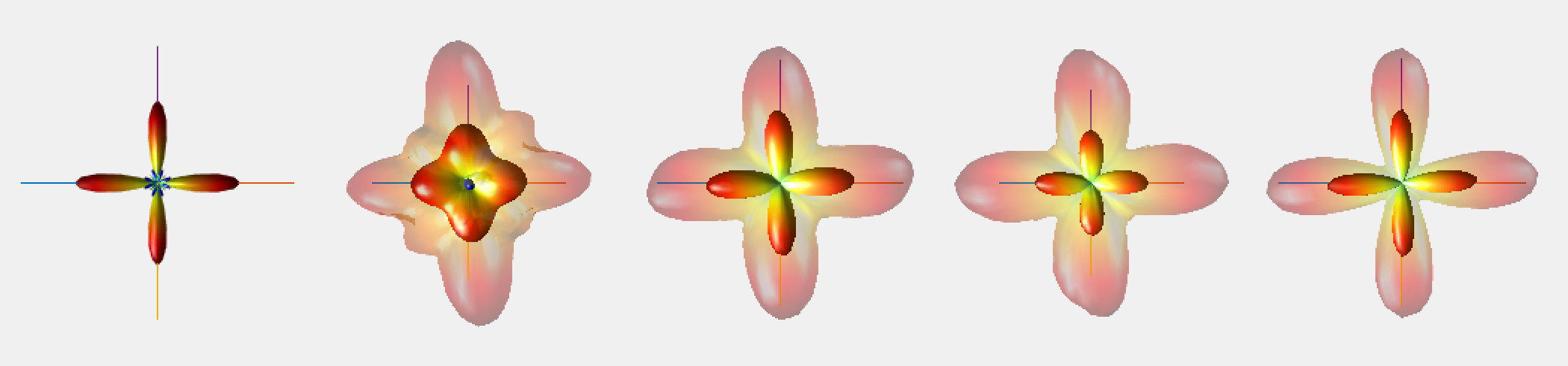
$75^{\circ}$
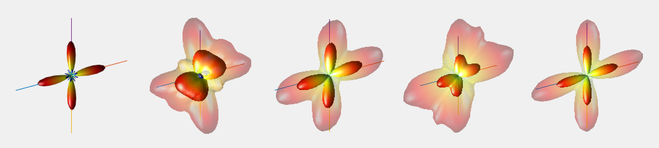
$60^{\circ}$

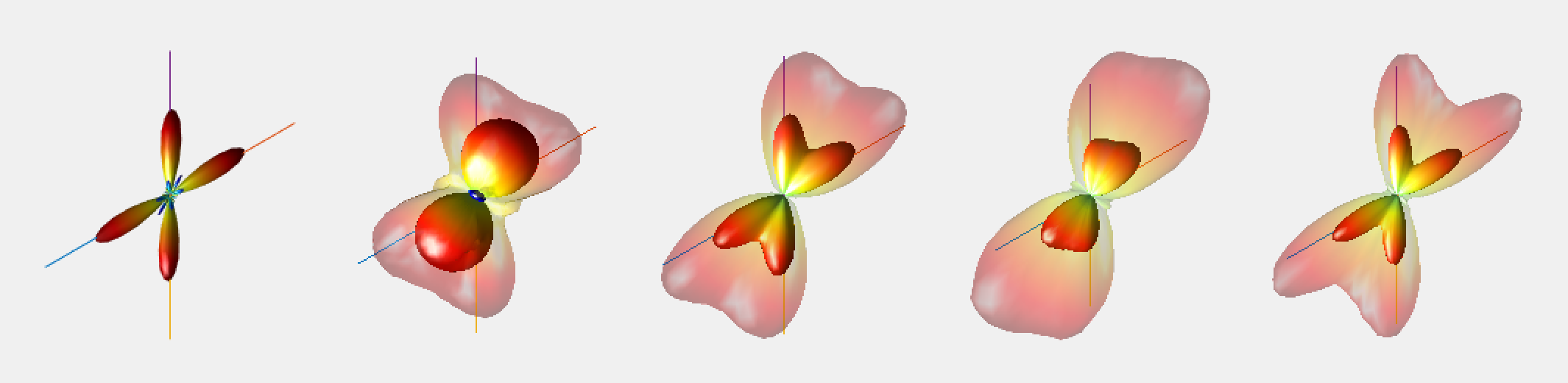
Figure 2: Two fiber crossing at $\mathbf{45^{\circ}}$ with $\mathbf{b=1000,3000s/mm^{2},SNR=20,50}$. $n=41$ gradient directions and $ratio=10$. The lines indicate the true fiber directions; the opaque part corresponds to mean estimated FOD across $100$ replicates; and the translucent part corresponds to mean plus two standard deviations of the estimated FOD.

	True FOD        SH-ridge        SCSD12           SCSD16             SN-lasso
	$b=1000s/mm^{2},SNR=20$
$45^{\circ}$
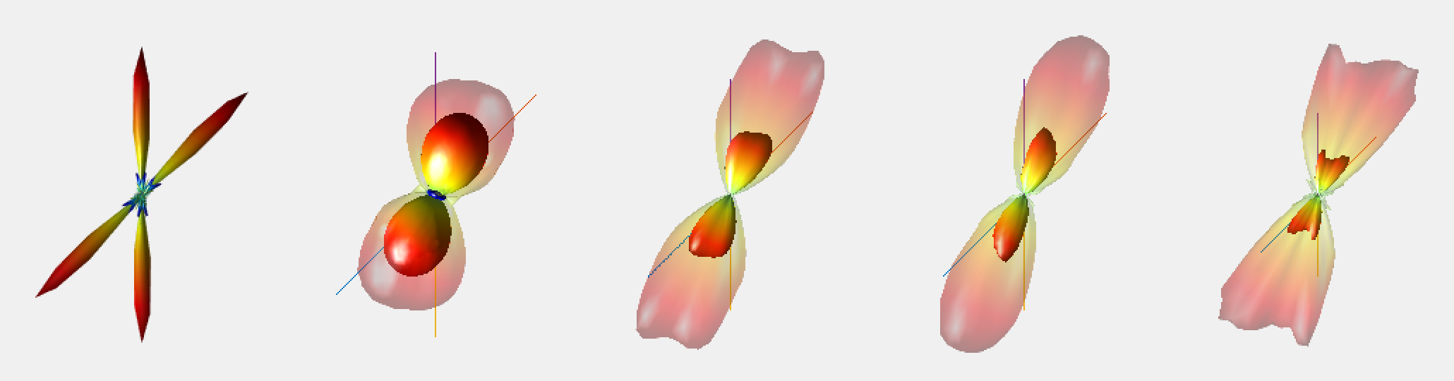
	$b=1000s/mm^{2},SNR=50$
$45^{\circ}$
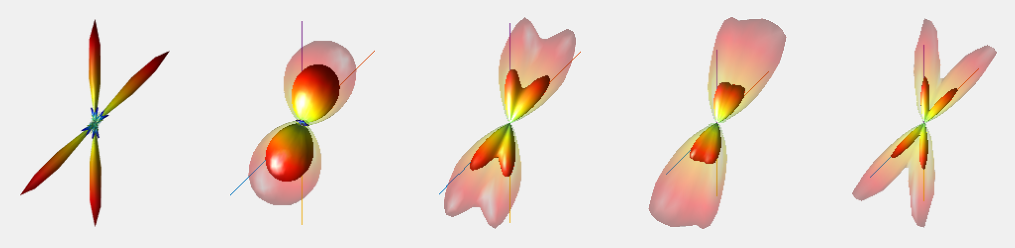
	$b=3000s/mm^{2},SNR=20$
$45^{\circ}$
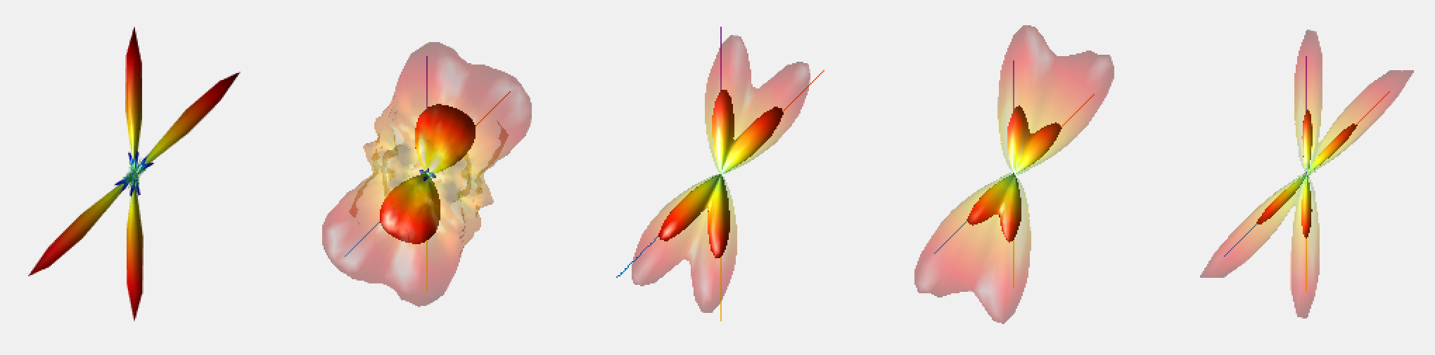
	$b=3000s/mm^{2},SNR=50$
$45^{\circ}$

Figure 3: Two fiber crossing at $\mathbf{45^{\circ}}$ with $\mathbf{b=1000,3000s/mm^{2},SNR=20,50}$. $n=41$ gradient directions and $ratio=10$.

(a) Angular error in direction estimation as percentage of the separation angle

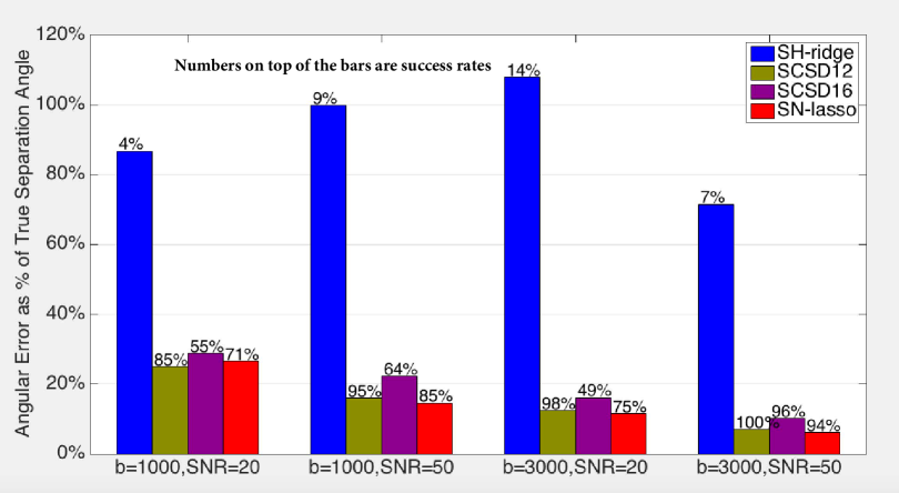
(b) Bias in separation angle estimation as percentage of the separation angle

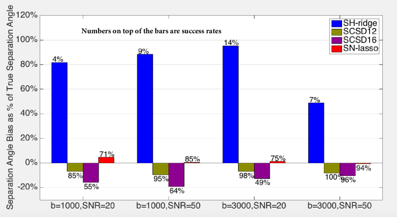
Figure 4: Two fiber crossing at $\mathbf{30^{\circ}}$ with $\mathbf{b=3000,5000s/mm^{2},SNR=20,50}$. $n=41$ gradient directions and $ratio=10$. The lines indicate the true fiber directions; the opaque part corresponds to mean estimated FOD across $100$ replicates; and the translucent part corresponds to mean plus two standard deviations of the estimated FOD.

	True FOD        SH-ridge        SCSD12           SCSD16             SN-lasso
	$b=3000s/mm^{2},SNR=20$
$30^{\circ}$
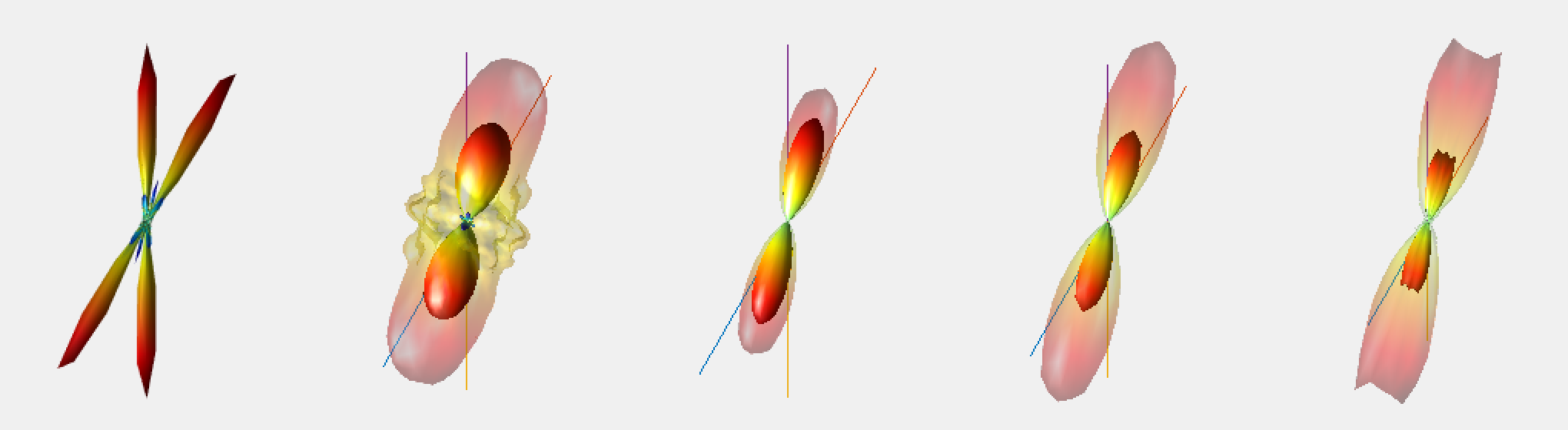
	$b=3000s/mm^{2},SNR=50$
$30^{\circ}$
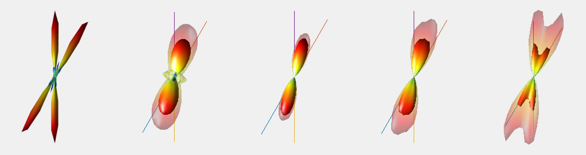
	$b=5000s/mm^{2},SNR=20$
$30^{\circ}$
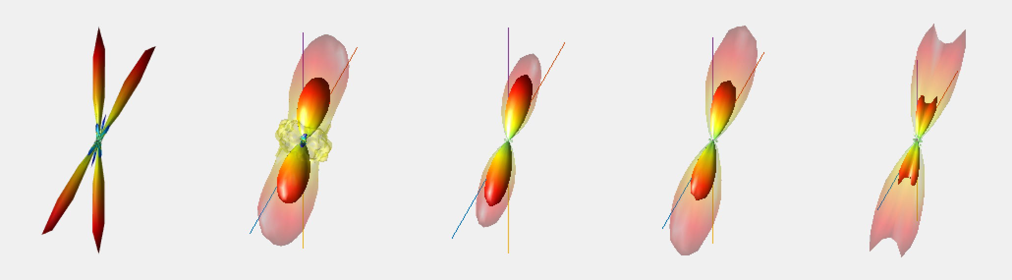
	$b=5000s/mm^{2},SNR=50$
$30^{\circ}$

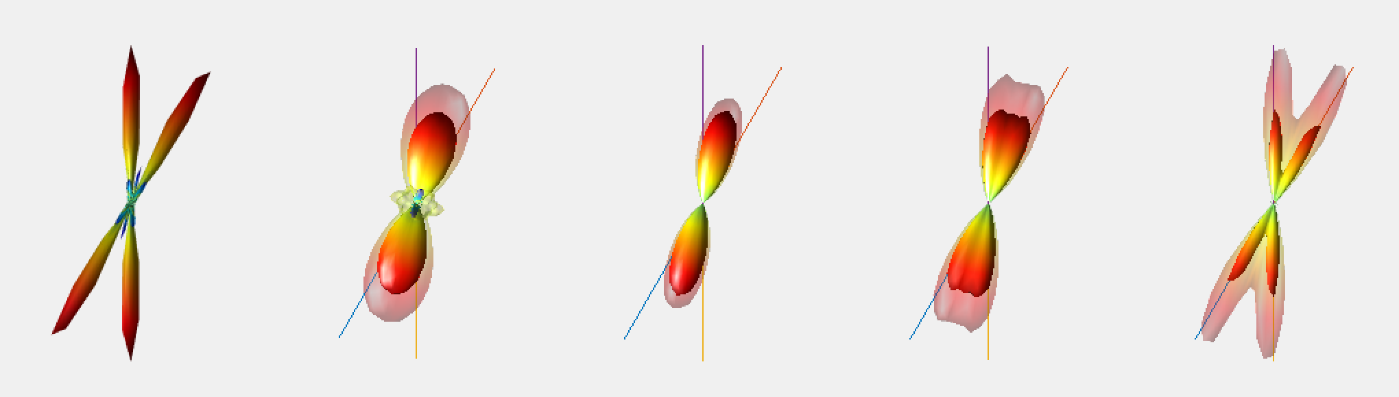
Figure 5: Two fiber crossing at $\mathbf{30^{\circ}}$ with $\mathbf{b=3000,5000s/mm^{2},SNR=20,50}$. $n=41$ gradient directions and $ratio=10$.

(a) Angular error in direction estimation as percentage of the separation angle

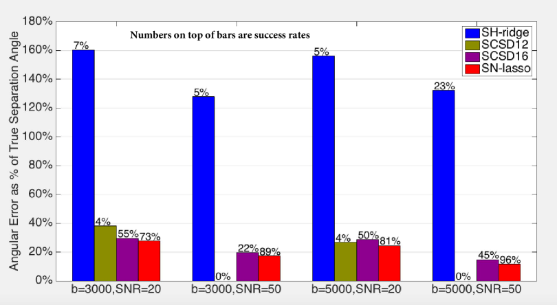
(b) Bias in separation angle estimation as percentage of the separation angle

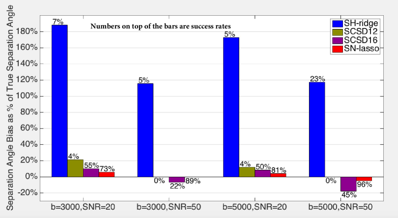
Additional results: impact of various experimental parameters

In addition to the 2-fiber setting, we also examine the isotropic ($K=0$), 1-fiber ($K=1$) and 3-fiber ($K=3$) cases. See Sections S.3.2.1, S.3.2.2 and S.3.2.7 in Supplementary Material, respectively. A crucial observation is that SN-lasso is able to automatically detect the isotropic diffusion by only selecting the constant function $\Phi_{00}$ and setting the coefficients of all the needlets to zero. In contrast, SCSD estimators result in noisy estimates of FOD with a number of spurious peaks of similar heights (Figure S.2; Table S.1). SN-lasso and SCSD estimators work well for the 1-fiber setting (i.e., no crossing), with nearly perfect success rates and small angular errors, whereas SH-ridge has significantly larger angular errors due to over-smoothing (Figure S.3 and Table S.2). For the 3-fiber crossing, SN-lasso again has visually the best FOD estimation and the highest overall success rate (Figures S.9, S.10, S.11; Tables S.10, S.11,S.12).

In terms of the impact of the number of gradient directions $n$, Figures 1 ($n=41$), S.5 ($n=81$), S.6 ($n=321$) and Tables S.3, S.6, S.7 indicate that, as $n$ increases, the variability of these estimators tends to decrease, the peak detection success rate tends to increase and the angular errors tend to decrease. In terms of the impact of the bvalue $b$, the performance of all these estimators improves dramatically when $b$ increases from $1000s/mm^{2}$ to $3000s/mm^{2}$ (sections S.3.2.6 and S.3.2.8) due to the larger contrast provided by larger bvalue. The relative performance of these estimators remains the same as previously discussed with SN-lasso leading to the best overall results.

3.2 Real D-MRI Data Experiments

We apply the FOD estimators to ROI I and the results are shown in Figure 6(b). It can be seen that, in the single fiber subregions, the SN-lasso estimates have sharp peaks consistent with the directions suggested by the fiber orientation colormaps. SCSD8 and SCSD12 are also able to preserve directionality pattern in such regions.

However, in the crossing fiber regions, SCSD estimators tend to be very noisy, while SH-ridge leads to overly smoothed estimates causing loss of directionality information. In contrast, SN-lasso is able to correctly resolve crossing patterns as evidenced by the following observations. From Figure 6 (a), it can be seen that voxels in columns 6 to 10 (from left) and rows 5 to 9 (from bottom) of ROI I have both small FA and MD values (dark on FA and MD maps). This is likely due to crossing fibers rather than being CSF since one defining feature of CSF is large MD values caused by faster water diffusion (Alexander et al.,, 2007). This is confirmed by the SN-lasso estimates (Figure 7(b), lower right panel) which show coherent fiber crossings in this subregion. The colormap suggests that these voxels represent fibers running in the left-to-right and into-to-out-of-the-page directions, in agreement with the SN-lasso estimates. On the other hand, the SCSD estimators result in FOD estimates that are incoherent among neighboring voxels and are with spurious peaks (Figure 7(b), upper right and lower left panels). We zoom into another subregion of ROI I (Figure 8), where the colormap indicates crossing between a horizontally orientated fiber (red-ish color) and a vertically orientated fiber (green-ish color) on the lower right corner. This is clearly captured by SN-lasso. The SCSD estimators again lead to noisy FOD estimates and SH-ridge estimates do not show clear directionality in this crossing region. A third subregion is examined by Figure S.14 of the Supplementary Material which shows similar phenomena.

Figure 6: ROI I. (a) From left to right: Fiber orientation colormap of the $z$-slice $40$: ROI I is indicated by the white box; Colormap, FA map and MD map of ROI I. (b): FOD estimates on ROI I: FA map is drawn on the background such that voxels with small FA values are shown by dark background color; Moreover, the size of the FOD estimates is modulated by mean diffusivity (MD): The larger the MD is, the smaller is the size of the depicted FOD estimate.

(a): Fiber orientation colormaps, FA map and MD map
Colormap of $z$-slice $40$  Colormap of ROI I       FA map of ROI I         MD map of ROI I
(b): FOD estimates on ROI I
SH-ridge	SCSD8
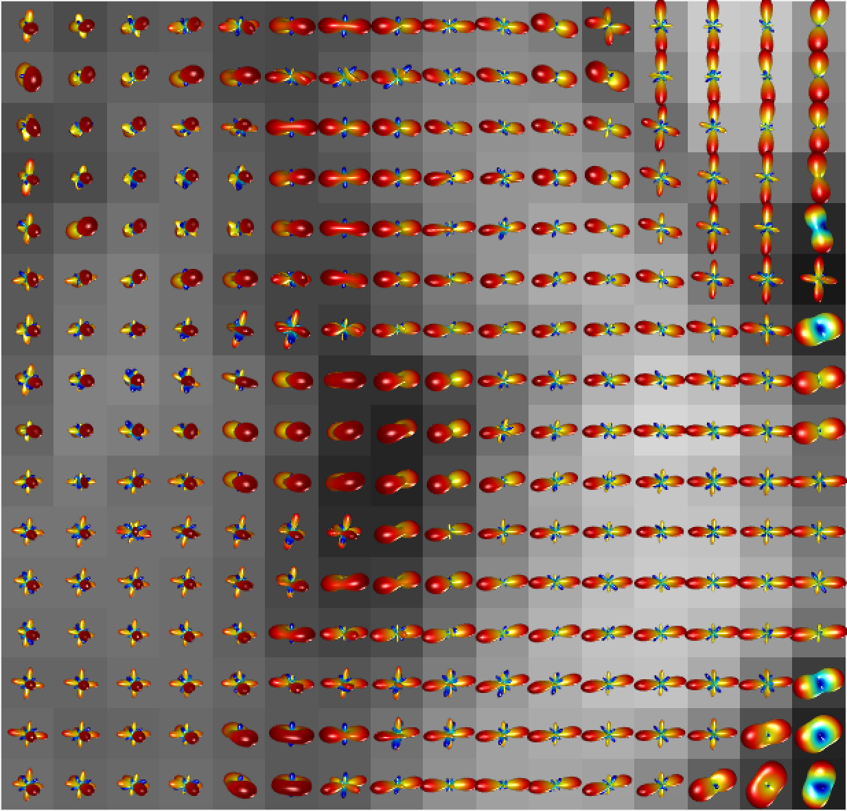
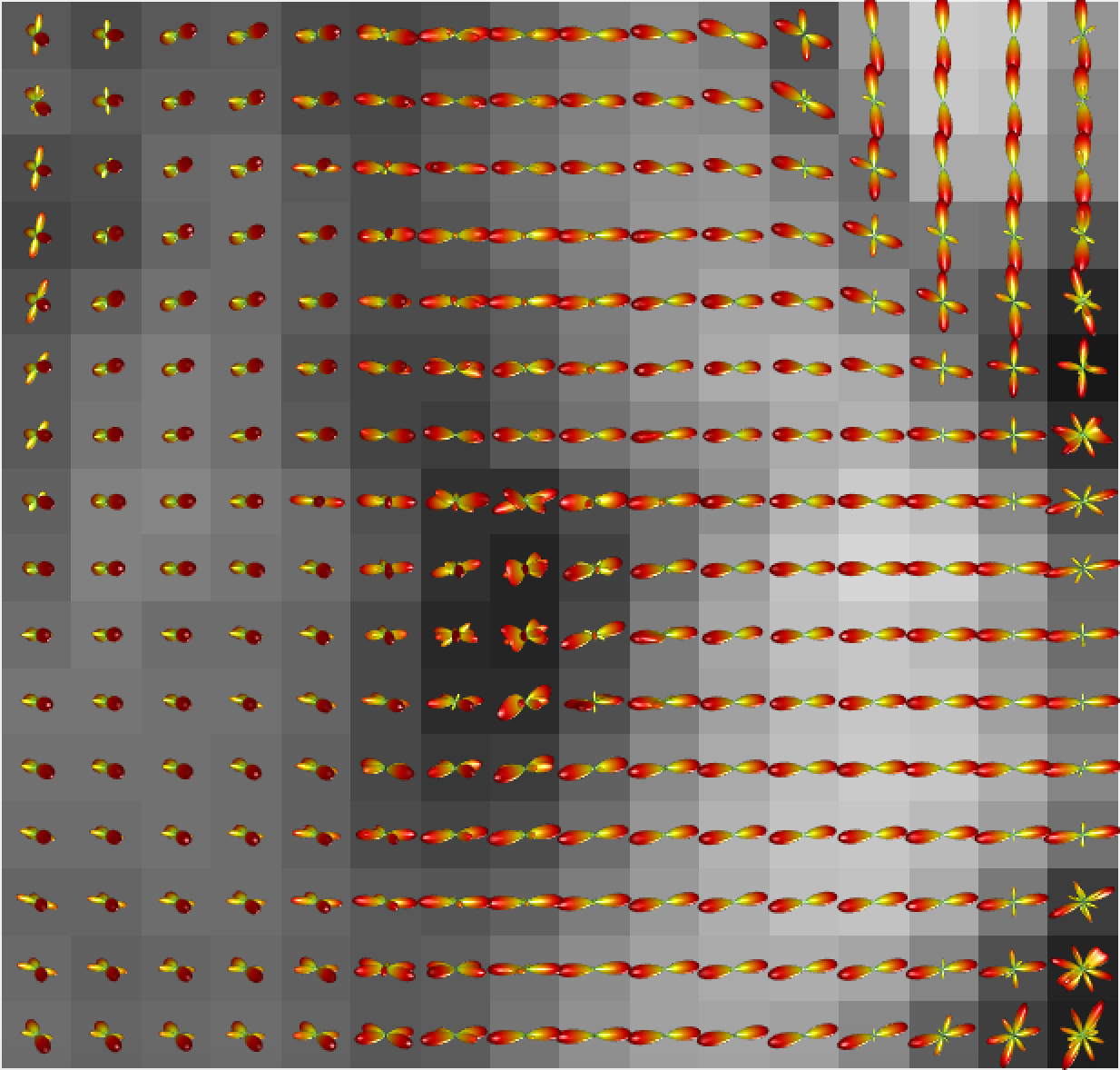
SCSD12	SN-lasso

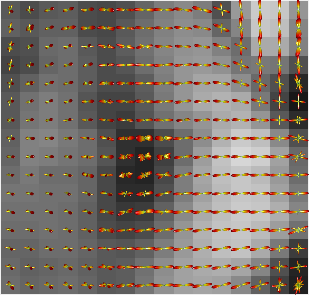
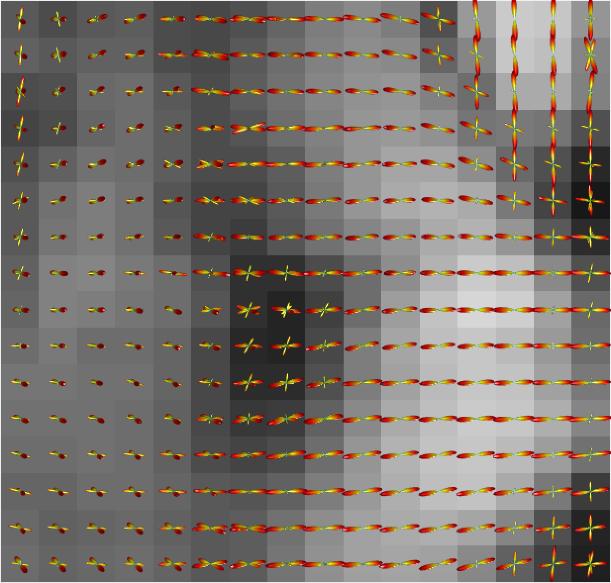
Figure 7: ROI I - Subregion 1: FOD estimates on a $5\times 5$ subregion (columns 6–10 and rows 5–9). This subregion is indicated by the white boxes on the colormap, FA map and MD map of ROI I.

(a): Fiber orientation colormaps, FA map and MD map
Colormap of $z$-slice $40$  Colormap of ROI I       FA map of ROI I         MD map of ROI I
(b): FOD estimates on the subregion indicated by the white box
SH-ridge	SCSD8
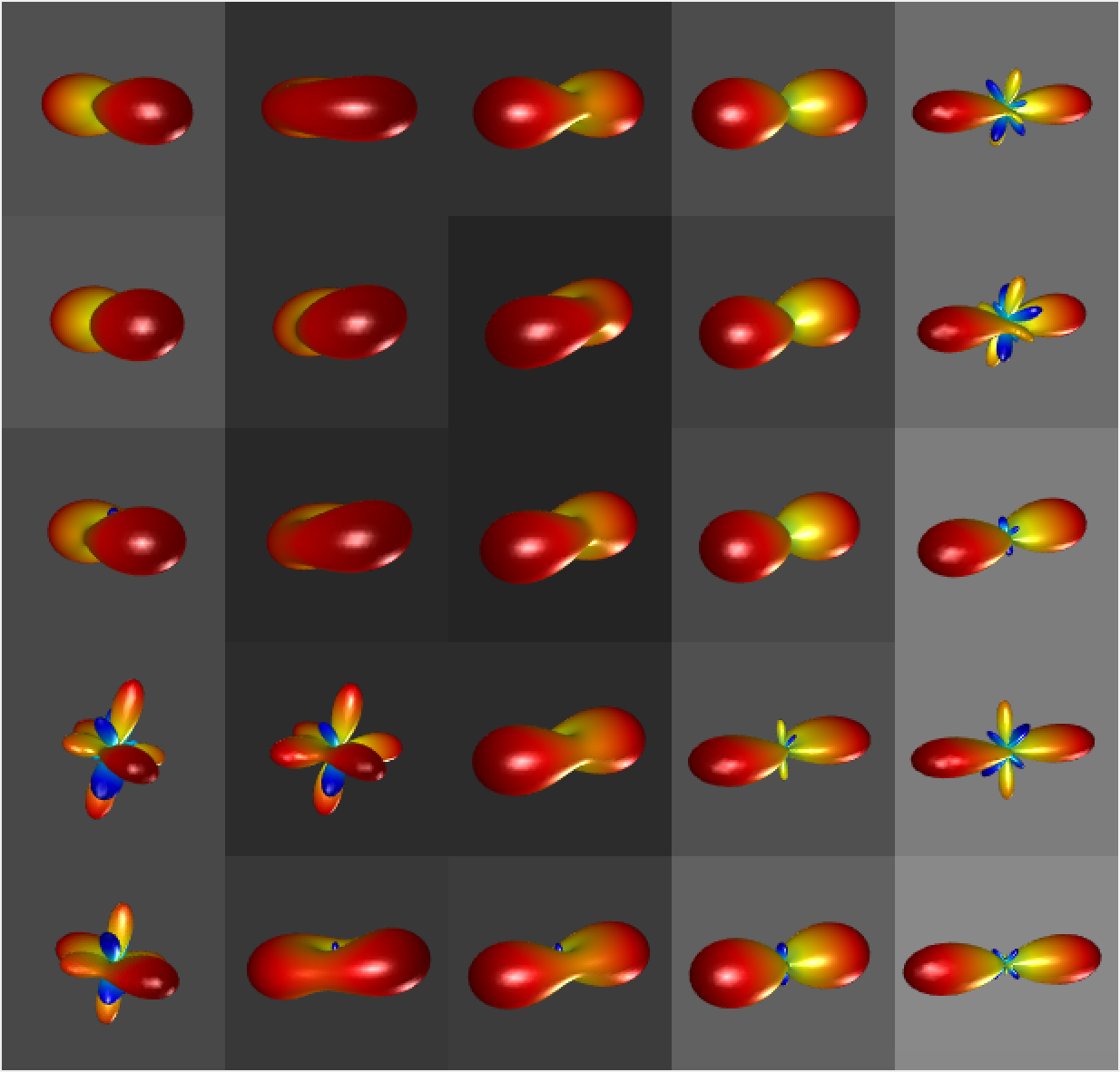
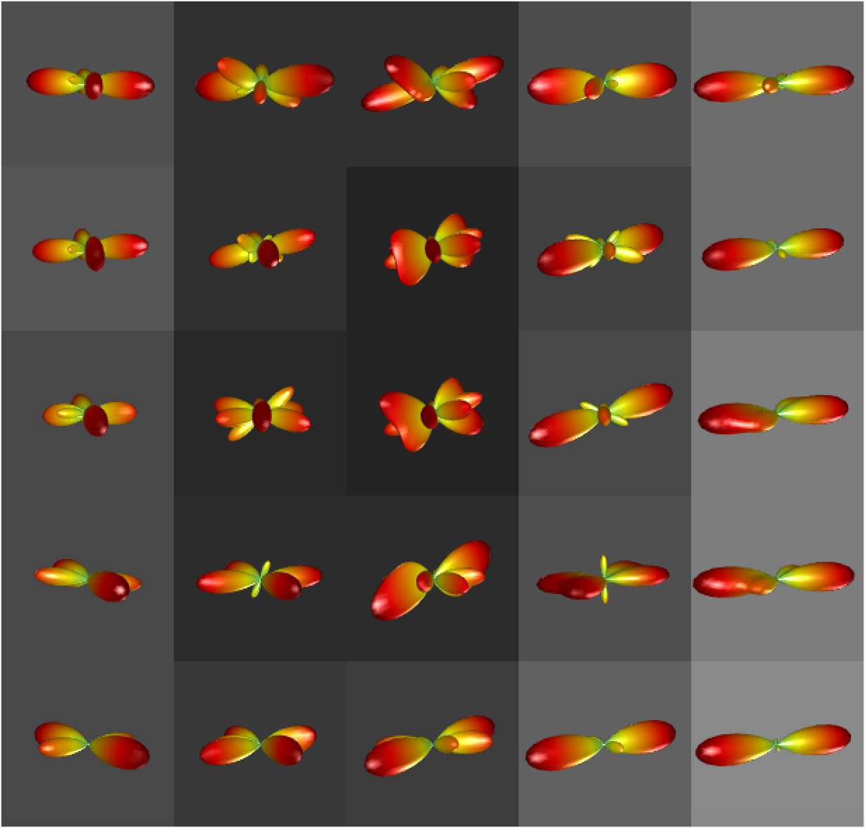
SCSD12	SN-lasso

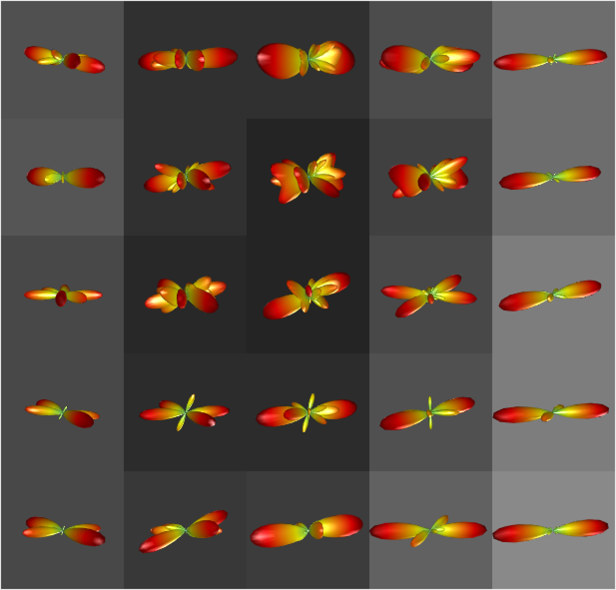
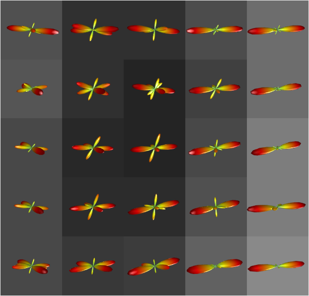
Figure 8: ROI I - Subregion 2: FOD estimates on a $5\times 5$ subregion (columns 12-16 and rows 1 - 5). This subregion is indicated by the white boxes on the colormap, FA map and MD map of ROI I.

(a): Fiber orientation colormaps, FA map and MD map
Colormap of $z$-slice $40$  Colormap of ROI I       FA map of ROI I         MD map of ROI I
(b): FOD estimates on the subregion indicated by the white box
SH-ridge	SCSD8
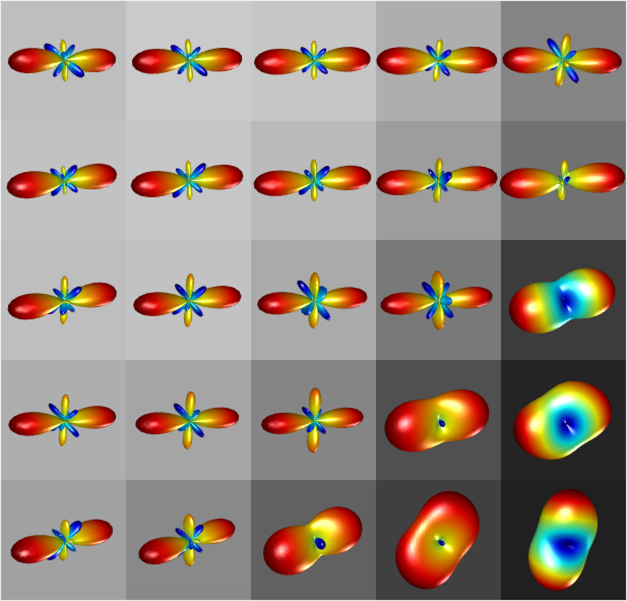
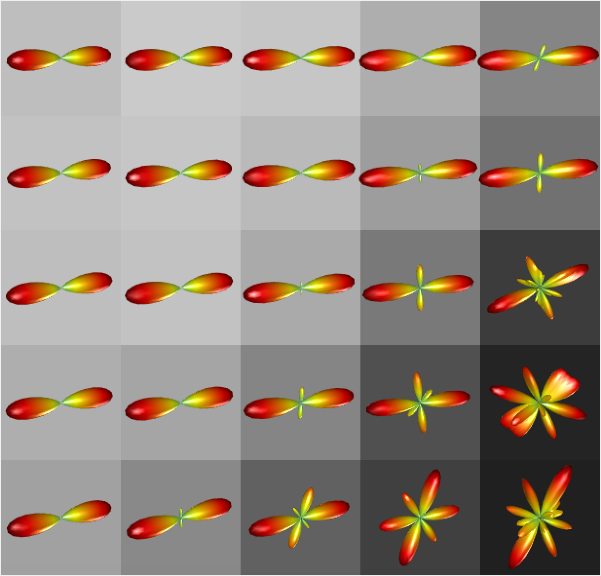
SCSD12	SN-lasso

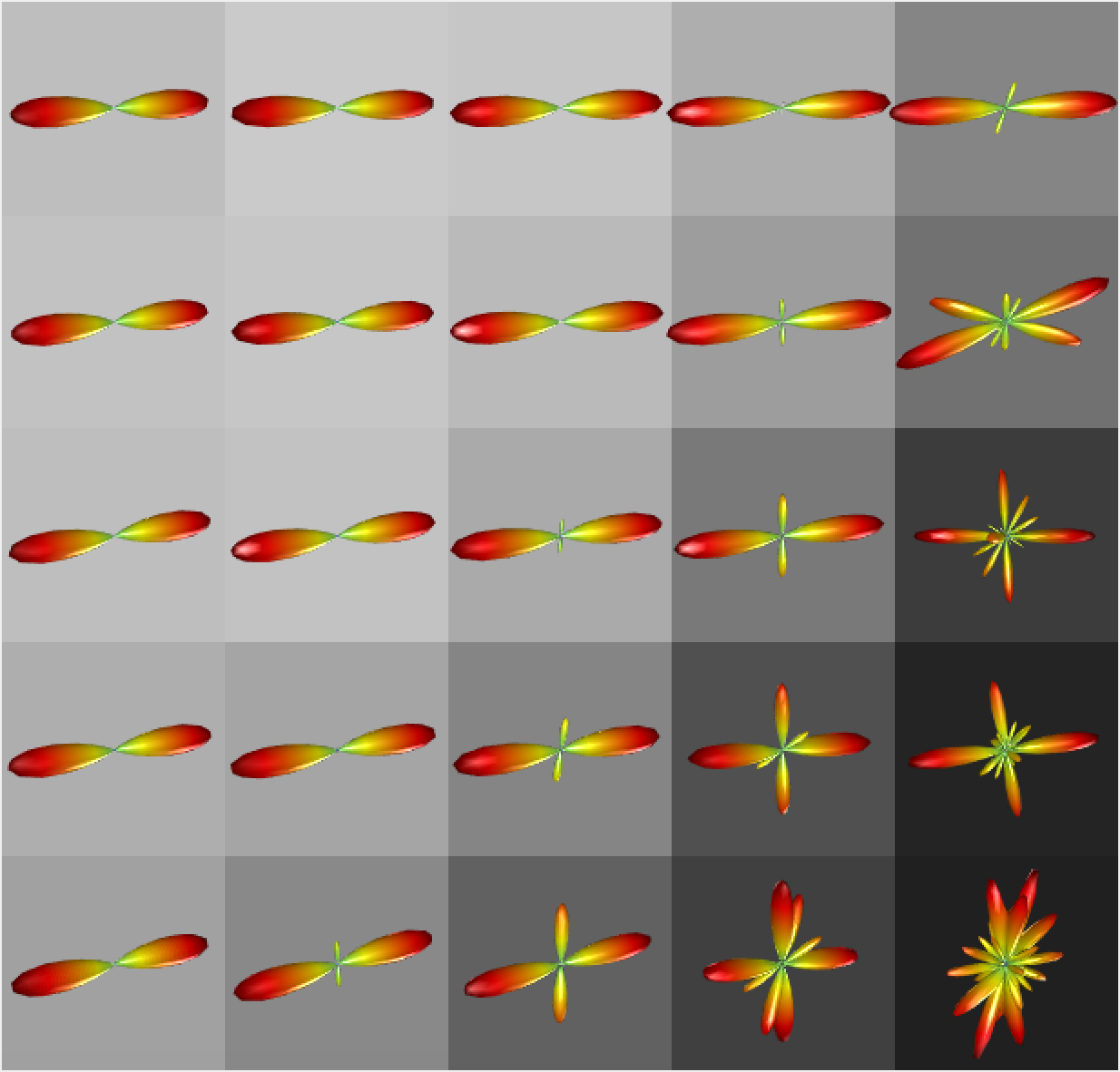
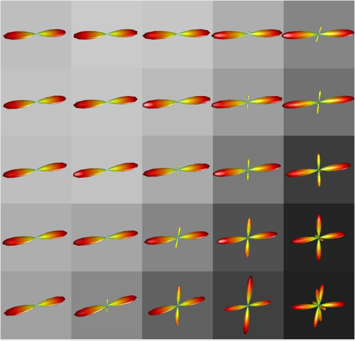
Figure 9: ROI II. (a) from left to right: Fiber orientation colormap of the $z$-slice $32$: ROI II is indicated by the white box; Colormap, FA map and MD map of ROI II. (b): FOD estimates on ROI II: FA map is drawn on the background such that voxels with small FA values are shown by dark background color; Moreover, the size of the FOD estimates is modulated by mean diffusivity (MD): The larger MD is, the smaller FOD estimate is depicted.

(a): Fiber orientation colormaps, FA map and MD map
Colormap of $z$-slice $32$  Colormap of ROI II       FA map of ROI II         MD map of ROI II
(b): FOD estimates on ROI II
SH-ridge	SCSD8
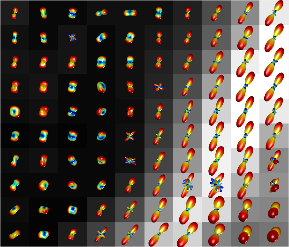
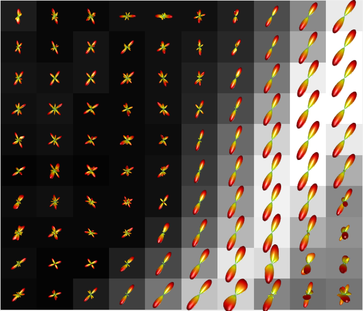
SCSD12	SN-lasso

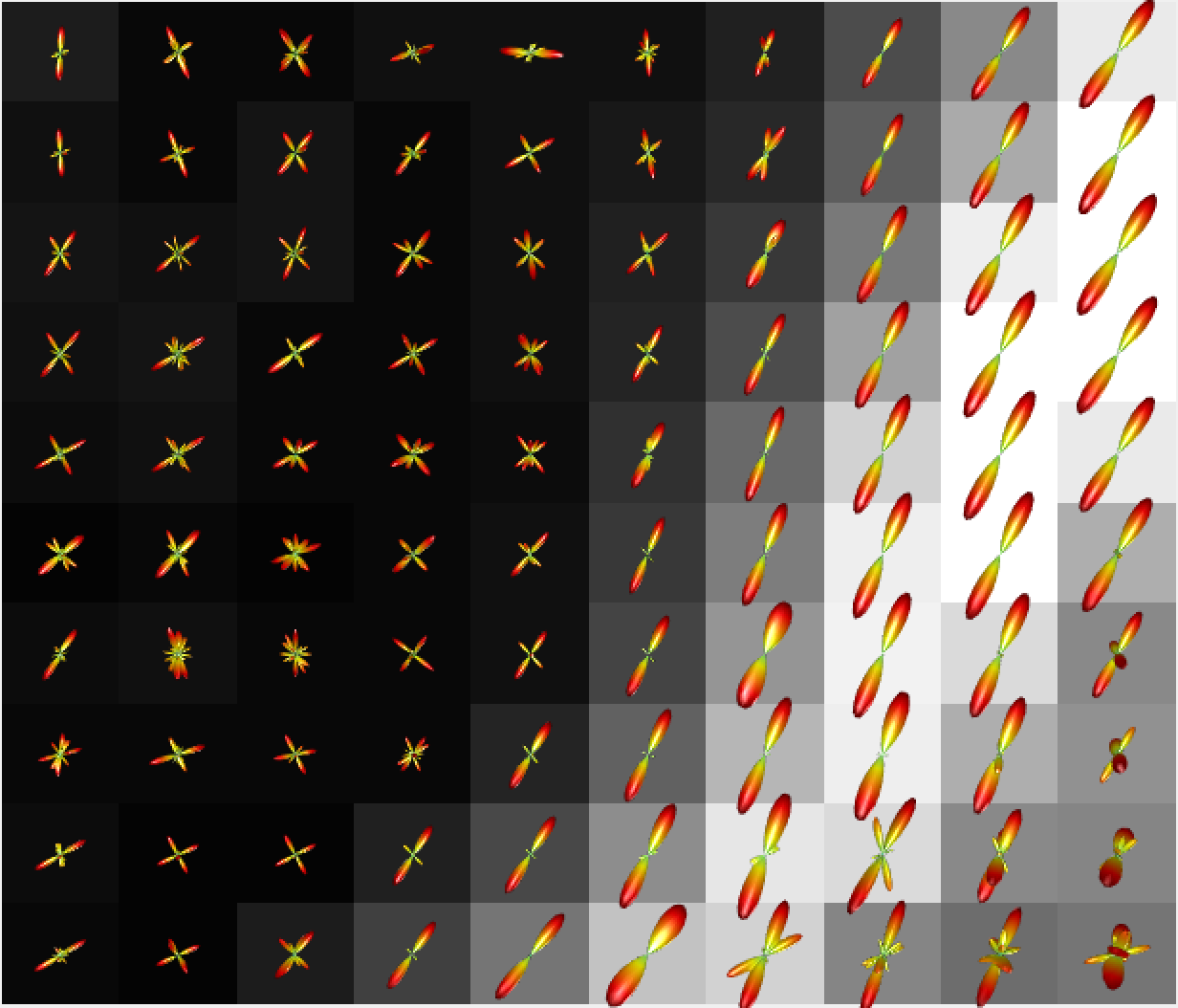
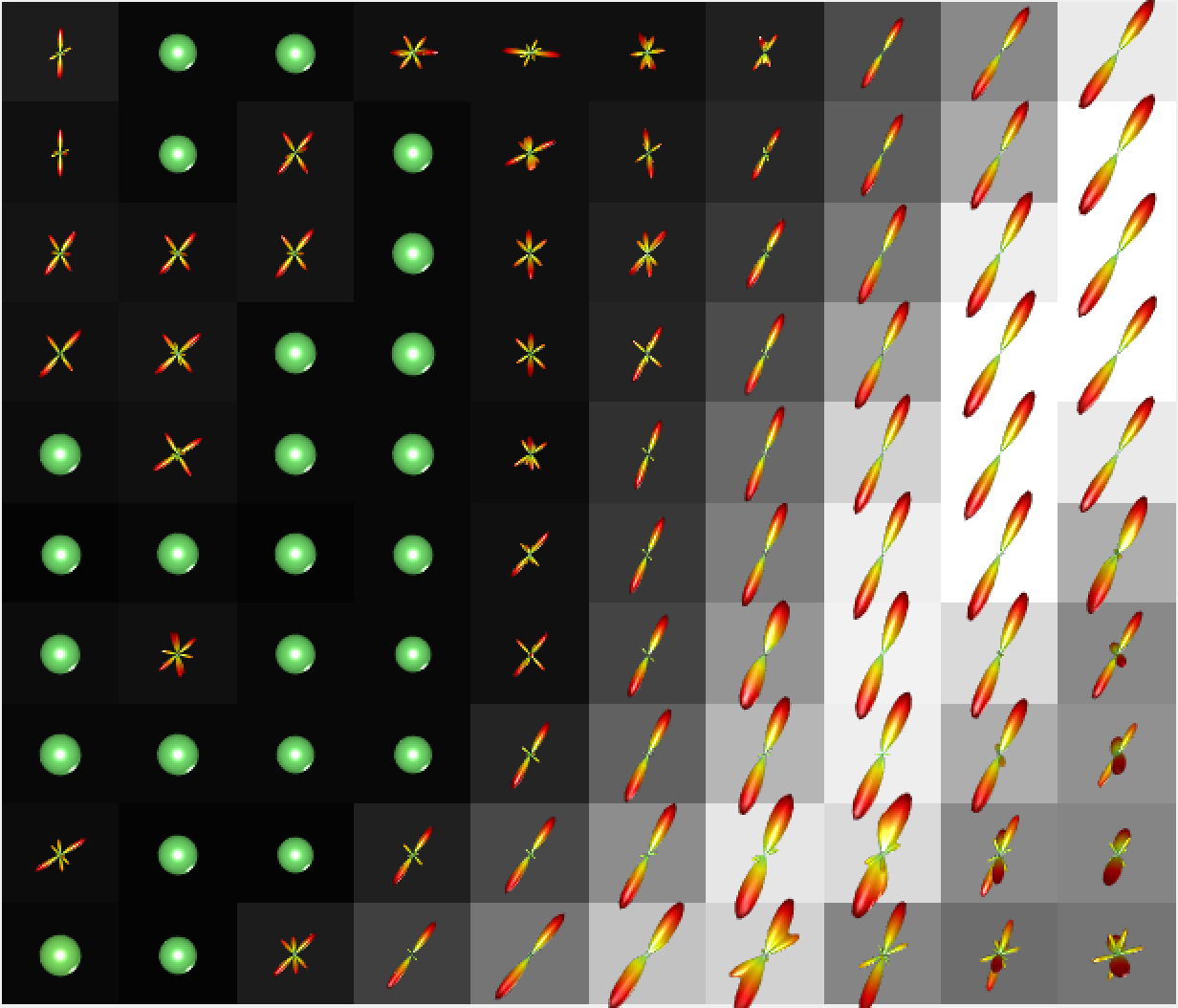
The upper left part of ROI II is likely to be CSF (Figure 9(a)), indicated by large MD values and small FA values (Alexander et al.,, 2007). This is corroborated by the SN-lasso estimates where FODs for many voxels in this subregion are estimated as being isotropic (represented by a green ball; Figure 9(b), lower right panel). In contrast, the other three estimators fail to identify any isotropic voxels in this subregion (Figure 9(b), the rest panels). The SN-lasso estimates also show clear single fiber in the lower right part of ROI II which is consistent with the bright greenish band on the colormap.

4 Discussion

In this paper, we present a novel method for estimating FOD that is accurate, has low variability and preserves sharp features, as well as being computationally efficient. The effectiveness of the proposed method derives from the utilization of multiresolution spherical frame called needlets that admits stable and parsimonious representation of FODs. Statistical efficiency, in terms of high accuracy and low variability in the estimates, is gained through imposing a sparsity constraint on the needlet coefficients, together with a nonnegativity constraint on the estimated FOD. The proposed method mitigates difficulties faced by two well-known FOD estimators, namely SH-ridge (Tournier et al.,, 2004) and SuperCSD (Tournier et al.,, 2007). Specifically, SH-ridge tends to over-smooth the peaks resulting in the loss of directionality information due to the global nature of the SH basis; and SuperCSD tends to amplify spurious peaks in estimated FODs due to high variability. On the other hand, the needlets frame used by the proposed method has excellent localization properties (in both frequency and space), and the $\ell_{1}$ penalized regression framework enables an adequate bias-variance trade off.

Experimental results on synthetic data suggest that the proposed method leads to better FOD estimation than two well known competing methods, particularly in terms of identification of major fiber directions. These results are consistent with the well-established statistical notion that a nonlinear shrinkage strategy allied with sparse representation is more efficient for signal recovery than a linear shrinkage strategy (Johnstone,, 2015; Tsybakov,, 2009).

The proposed method is able to successfully reconstruct an FOD when the fiber crossing angle is as small as $30^{\circ}$ provided that the bvalue and SNR are sufficiently large (e.g., $b=3000,5000s/mm^{2},SNR=50$). Resolving small crossing angles at relatively low bvalues has been reported in literature to be a challenging setting. For example, in Yeh and Tseng, 2013b , under $b=1500s/mm^{2},SNR=20,n=55$, the best performing method has around $20^{\circ}$ angular deviation at $45^{\circ}$ crossing. On the other hand, with the fast advancement of D-MRI technologies, we are expecting larger bvalue and SNR (Setsompop et al.,, 2013; Van Essen et al.,, 2013). Use of larger bvalue for reconstruction of diffusion characteristics has also been previously advocated in the literature (Jensen et al.,, 2016; Jones et al.,, 2013; Roine et al.,, 2015). Therefore, the proposed method holds great promise in resolving even subtle fiber crossing patterns. Moreover, the proposed method has the distinct advantage of being able to identify isotropic diffusion with very high degrees of accuracy.

Another important insight gained from these experiments is that, for the representations considered in this paper, employing larger bvalue is more effective than using larger number of gradient directions for the purpose of distinguishing among multiple fiber bundles with relatively small crossing angles. The observations gained here may be used as a guideline for specifying the acquisition parameters in future D-MRI experiments.

The proposed method is also examined through a real data experiment that uses D-MRI data sets from the second phase of the ADNI project. It leads to realistic descriptions of crossing fibers with less noise than competing methods at a relatively low number of gradient directions, indicating practical value of our method for analyzing D-MRI data from many large scale studies.

Our use of a multiresolution spherical wavelets bears some similarity with the dODF-sharpening strategy of Kezele et al., (2010) where a spherical wavelets transform due to Starck et al., (2006) is employed. However, the method of Kezele et al., (2010) is not directly applicable here since we aim to estimate the FOD (or fiber ODF) rather than dODF. Moreover, the spherical wavelets constructed by Starck et al., (2006) do not possess the spherical function representation characteristics and tight frame properties of needlets. Finally, unlike our method, where the needlets representation enables us to impose sparsity constraints, Kezele et al., (2010) use the spherical wavelets transform only as a band-pass filter. Among alternative choices of spherical wavelets, the lifting scheme based wavelets constructed by Schröder et al., (1995) provide excellent spatial localization and ease of computation. However, since these wavelets are nonsmooth and consequently poorly localized in frequency, they are not optimal for FOD reconstruction since FODs have sharp localized features, which require frequency localization of the basis functions for a parsimonious representation.

A key avenue for future research is the extension of this method to multiple $q$-shell data. An emerging strength of such data is its ability to accommodate multiple cellular compartment models that separately quantify the contributions of free water, water bound within the myelin sheath, inter-axonal water, and other compartments to the D-MRI signal. As such, multiple $q$-shell data may be best modeled to allow for different FOD representations for different compartments, as in the NODDI scheme (Zhang et al.,, 2012), rather than a single unified spherical function as here. On the other hand, spherical needlets might provide accurate and robust representation of some of these signal components, possibly with specific coefficient penalties for specific components. Future experimentation should determine settings in which spherical needlets are useful for modeling components of the multiple $q$-shell D-MRI signal.

While estimating the FOD at a voxel, our method only uses data from the same voxel. Since there is a natural connection between local fiber orientation and the shape of FODs, we may consider the incorporation of neighboring voxel data in the estimation of FODs to further improve statistical efficiency. We also want to conduct inferences such as constructing confidence balls for the estimated FODs, for which we shall build upon principles of resampling and recent developments in post-model-selection inference (Lockhart et al.,, 2014; Lee et al.,, 2016; Tibshirani et al.,, 2015). Lastly, needlet representation can be extended to estimate other D-MRI related objects such as ODFs which are also spherical functions with sharp features. Thus we expect to see many applications and extensions of the techniques proposed in this paper.

Supplementary Material for “Estimating fiber orientation distribution from diffusion MRI with spherical needlets”

S.1 Symmetrized needlets and the design matrix

Let $\{\Phi_{lm};l=0,1,2,\ldots;m=-l,-l+1,\ldots,l-1,l\}$ denote the complex-valued SH functions where $l$ denotes the harmonic order and $m$ denotes the phase order. It forms an orthonormal basis for the square integrable complex functions on the unite sphere $\mathbb{S}^{2}$. The real symmetrized SH functions are defined as follows (Descoteuax et al.,, 2007). For $l=0,2,4,\ldots$ and $m=-l,-l+1,\ldots,l-1,l$

$$\widetilde{\Phi}_{lm}=\begin{cases}\sqrt{2}\cdot\text{Re}\big{(}\Phi_{lm}\big{)},&\text{if}\ -l\leq m<0\\ \Phi_{l0},&\text{if}\ m=0\\ \sqrt{2}\cdot\text{Img}\big{(}\Phi_{lm}\big{)},&\text{if}\ 0<m\leq l\end{cases},$$ (S.1)

where $\text{Re}\big{(}\Phi_{lm}\big{)}$ and $\text{Img}\big{(}\Phi_{lm}\big{)}$ are the real and imaginary parts of $\Phi_{lm}$, respectively. The real symmetrized SH functions form an orthonormal basis for the square integrable real symmetric functions on the unit sphere.

Let $\{\zeta_{jk}\}$ denote the quadrature points according to the HEALPix construction of spherical needlets and $\{\widetilde{\psi}_{jk}\}$ denote the needlet functions. The symmetrized needlet functions can be easily constructed utilizing the following two facts: (i) For each level $j$, the quadrature points appear in pairs that are symmetric to the origin, i.e. for each $k$, there is a $k^{\prime}$ such that $\zeta_{jk^{\prime}}=-\zeta_{jk}$. (ii) The needlet functions corresponding to the pair of symmetric quadrature points satisfy $\widetilde{\psi}_{jk}(\mathbf{x})=\widetilde{\psi}_{jk^{\prime}}(-\mathbf{x})$ for $\mathbf{x}\in\mathbb{S}^{2}$. The symmetrized needlets is defined as follows:

$$\psi_{jk}(\mathbf{x})=\frac{1}{2}\big{(}\widetilde{\psi}_{jk}(\mathbf{x})+\widetilde{\psi}_{jk^{\prime}}(\mathbf{x})\big{)},~{}~{}\zeta_{jk}\in\mathbb{S}^{2}_{+}.$$

Real symmetric SH functions and symmetrized needelts corresponding to various frequency levels are depiected in Figure S.1.

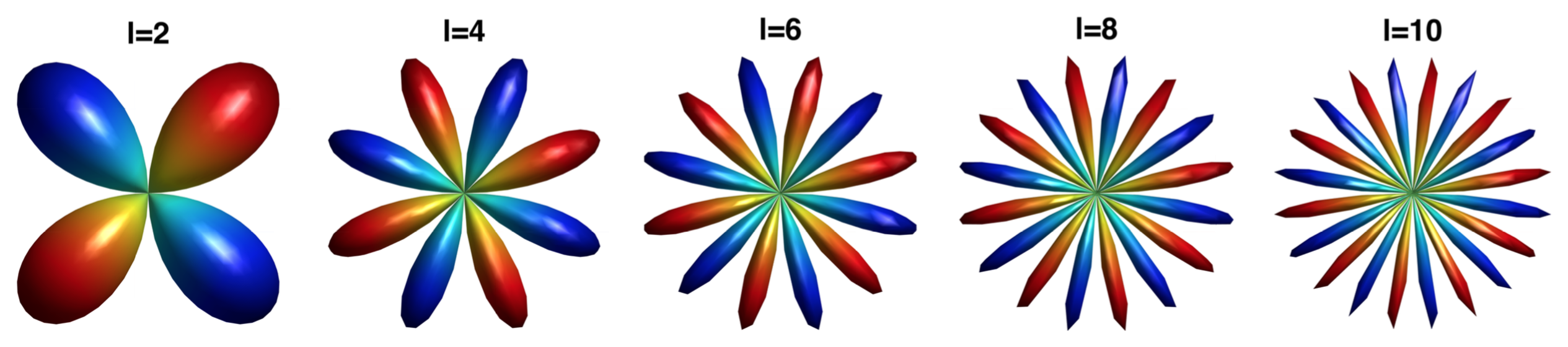
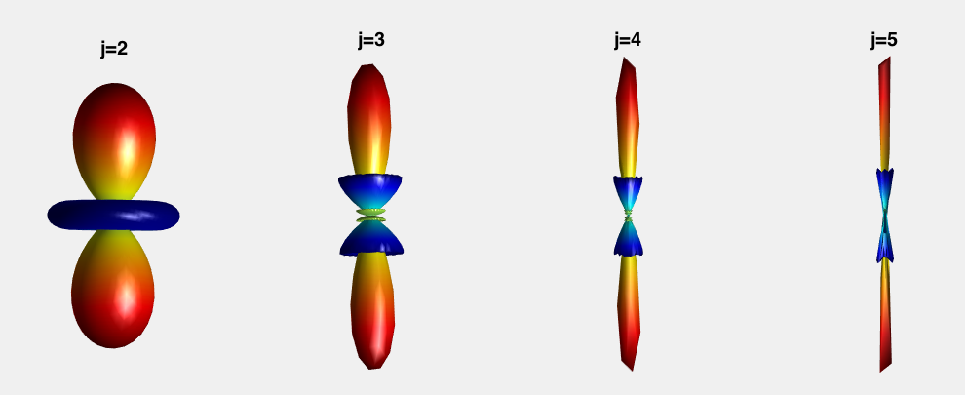
Figure S.1: Left panel: Real symmetric spherical harmonics; Right Panel: Real symmetric spherical needlets.

Recall that $\Phi_{00}$, the constant function on unit sphere, is included to make the needlets frame tight. Hence the total number of basis functions in the (symmetried) needlets frame up to the frequency level $j_{max}$ is $1+\frac{1}{2}\sum_{j=1}^{j_{max}}N_{j,pix}$, where $N_{j,pix}$ is the number of spherical needlets at frequency level $j$ and $N_{j,pix}=12\times(2^{j-1})^{2}$ according to the HEALPix construction of spherical needlets.

Let $\mathbf{\Phi}_{l}$ denote the vector consisting of real symmetric SH functions upto level $l$ and $\mathbf{\Psi}_{j}$ denote the vector consisting of real symmetric spherical needlets (SN) functions upto level $j$. Let $L_{l}=|\mathbf{\Phi}_{l}|$ and $N_{j}=|\mathbf{\Psi}_{j}|$. Let $\mathbb{SH}_{l}$ and $\mathbb{SN}_{j}$ denote the linear space generated by $\mathbf{\Phi}_{l}$ and $\mathbf{\Psi}_{j}$, respectively.

For $l_{\max}\geq 1$, let $j_{max}=\lceil\log_{2}(l_{\max})+1\rceil$. For example, when $l_{\max}=8$ ($L=45$ SH basis functions), the corresponding $j_{\max}=4$ ($N=511$ needlets). Then by needelt construction (equation (2) of the main text):

$$\mathbb{SH}_{l_{\max}}\leq\mathbb{SN}_{j_{\max}}\leq\mathbb{SH}_{l_{\max+1}},~{}~{}~{}L:=L_{l_{\max}}<N:=N_{j_{\max}}<\tilde{L}:=L_{l_{\max}+1}.$$

where “$\leq$” stands for the “subspace” symbol.

If a spherical function $F\in\mathbb{SH}_{l_{\max}}$, then it can be linearly represented by all three collections $\mathbf{\Phi}_{l_{\max}},\mathbf{\Psi}_{j_{\max}},\mathbf{\Phi}_{l_{\max+1}}$. Denote their respective coefficients as $\mathbf{f},\boldsymbol{\beta},\mathbf{\tilde{f}}$. Note that the needlet coefficients $\boldsymbol{\beta}$ are defined through inner products according to equation (3) of the main text. (As needlets are not linearly independent, linear representation in needlets is not unique and thus we need to explicitly define the needlet coefficients.)

Since $\mathbb{SN}_{j_{\max}}\leq\mathbb{SH}_{l_{\max+1}}$, $\mathbf{\Psi}_{j_{\max}}$ can be linearly represented by $\mathbf{\Phi}_{l_{\max}+1}$:

$$\mathbf{\Psi}_{j_{\max}}=\mathbf{\tilde{C}}_{N\times\tilde{L}}\mathbf{\Phi}_{l_{\max}+1}.$$

Thus, $\boldsymbol{\beta}_{N\times 1}=\mathbf{\tilde{C}}_{N\times\tilde{L}}\mathbf{\tilde{f}}_{\tilde{L}\times 1}.$

Moreover, due to orthogonality of the SH functions, $\mathbf{\tilde{f}}^{T}=(\mathbf{f}^{T},\mathbf{0}^{T})$. Let $\mathbf{C}^{\ast}$ denote the matrix consisting of the first $L$ columns of $\mathbf{\tilde{C}}$, then

$$\boldsymbol{\beta}_{N\times 1}=\mathbf{C}^{\ast}_{N\times L}\mathbf{f}_{L\times 1}.$$

Note that $rank(\mathbf{C}^{\ast})=L$, and thus

$$\mathbf{f}_{L\times 1}=\mathbf{C}_{L\times N}\boldsymbol{\beta}_{N\times 1},$$

with

$$\mathbf{C}=(\mathbf{C}^{\ast,T}\mathbf{C}^{\ast})^{-1}\mathbf{C}^{\ast,T}$$

being the transition matrix from needlet coefficients to SH coefficients. Finally, the first $L$ SH coefficients of the first $N$ needlets, $\mathbf{C}^{\ast}$, can be computed analytically according to the needlets construction formula equation (2) of the main text.

S.2 Algorithms details

S.2.1 The ADMM algorithm

We describe the ADMM algorithm (Boyd et al.,, 2011) for non-negativity constrained $\ell_{1}$ penalization problem in this section. For

$$x\in\mathbb{R}^{n},\;A\in\mathbb{R}^{m\times n},\;b\in\mathbb{R}^{m},\;C\in\mathbb{R}^{l\times n}\;\textrm{and}\;d\in\mathbb{R}^{l},$$

the constrained lasso problem can be formulated as:

$${\rm argmin}_{x:Cx\leq d}\frac{1}{2}||Ax-b||_{2}^{2}+\lambda||x||_{1}.$$

The corresponding ADMM form of this problem is to minimize:

$$\frac{1}{2}||Ax-b||_{2}^{2}+\lambda||z||_{1}+I_{+}(w)$$

subject to

$$x-z=0,\quad Cx+w-d=0,$$

where $z\in\mathbb{R}^{n}$, $w\in\mathbb{R}^{l}$, $I_{+}(w)=0$ if $w\geq 0$(elementwise) and $I_{+}(w)=\infty$ if otherwise.

The augmented Lagrangian has the form:

$$L_{\rho}(x,z,w,u,t)=\frac{1}{2}||Ax-b||_{2}^{2}+\lambda||z||_{1}+I_{+}(w)+\frac{\rho}{2}||x-z+u||_{2}^{2}+\frac{\rho}{2}||Cx+w-d+t||_{2}^{2},$$

where $u\in\mathbb{R}^{n}$ and $t\in\mathbb{R}^{l}$.

The ADMM algorithm performs iterative updates as follows:

• x-minimization

  • $x^{k+1}=\arg\min_{x}\frac{1}{2}||Ax-b||_{2}^{2}+\frac{\rho}{2}||x-z^{k}+u^{k}||_{2}^{2}+\frac{\rho}{2}||Cx+w^{k}-d+t^{k}||_{2}^{2}$.

    • $x^{k+1}=\left(A^{T}A+\rho I_{n}+\rho C^{T}C\right)^{-1}\left(A^{T}b+\rho\left(z^{k}-u^{k}\right)+\rho C^{T}\left(d-w^{k}-t^{k}\right)\right)$, when $m+l\geq n$.

    • $x^{k+1}=\rho^{-1}\left[I_{n}-B^{T}\left(BB^{T}+\rho I_{m+l}\right)^{-1}B\right]\left(A^{T}b+\rho\left(z^{k}-u^{k}\right)+\rho C^{T}\left(d-w^{k}-t^{k}\right)\right)$, where $B=\left(\begin{array}[]{c}A\\ \sqrt{\rho}C\end{array}\right)\in\mathbb{R}^{(m+l)\times n}$, when $m+l<n$.

• z/w-minimization

  • $z^{k+1}=\arg\min_{z}\frac{\rho}{2}||x^{k+1}+u^{k}-z||_{2}^{2}+\lambda||z||_{1}=S_{\lambda/\rho}(x^{k+1}+u^{k})$,
    where $S_{\lambda/\rho}(x^{k+1}+u^{k})_{i}=(|x^{k+1}_{i}+u^{k}_{i}|-\frac{\lambda}{\rho})_{+}\textrm{sign}(x^{k+1}_{i}+u^{k}_{i})$.

  • $w^{k+1}=\arg\min_{w}\frac{\rho}{2}||w+Cx^{k+1}-d+t^{k}||_{2}^{2}+I_{+}(w)=\max\left\{0,\;-Cx^{k+1}+d-t^{k}\right\}$,
    where the maximum is taken elementwisely.

• dual-update

  • $u^{k+1}=u^{k}+x^{k+1}-z^{k+1}$.

  • $t^{k+1}=t^{k}+Cx^{k+1}+w^{k+1}-d$.

The stopping criterion of the algorithm is as follows :

• $||r^{k}||_{2}=\left(||x^{k}-z^{k}||_{2}^{2}+||Cx^{k}+w^{k}-d||_{2}^{2}\right)^{\frac{1}{2}}$.

• $||s^{k}||_{2}=\rho||z^{k}-z^{k-1}-C^{T}\left(w^{k}-w^{k-1}\right)||_{2}$.

• $\epsilon^{\textrm{pri}}=\sqrt{n+l}\epsilon^{\textrm{abs}}+\epsilon^{\textrm{rel}}\max\left\{\left(||x^{k}||_{2}^{2}+||Cx^{k}||_{2}^{2}\right)^{\frac{1}{2}},\left(||z^{k}||_{2}^{2}+||w^{k}||_{2}^{2}\right)^{\frac{1}{2}},||d||_{2}\right\}$.

• $\epsilon^{\textrm{dual}}=\sqrt{n}\epsilon^{\textrm{abs}}+\epsilon^{\textrm{rel}}\rho||u^{k}+C^{T}t^{k}||_{2}$.

• Terminate when $||r^{k}||_{2}\leq\epsilon^{\textrm{pri}}$ and $||s^{k}||_{2}\leq\epsilon^{\textrm{dual}}$.

We set $\epsilon^{\textrm{abs}}=10^{-4}$ and $\epsilon^{\textrm{rel}}=10^{-2}$ to strike a good balance between convergence time and accuracy. We also set $\rho=\lambda$ following the suggestions in (Boyd et al.,, 2011).

S.2.2 Choice of penalty parameter

We consider a criterion that is based on the residual sum of squares (RSS). Note that, $RSS$ itself is not able to achieve bias-variance trade-off: It will always lead to the largest model (i.e., selecting the smallest $\lambda$). Instead, we choose the largest $\lambda$ where the RSS starts to flatten out. Specifically, we fit model (9) with a sequence of decreasing $\lambda$s on a grid $\Lambda=\{\lambda_{1}>\cdots>\lambda_{K}\}$ and calculate $RSS_{k}$ and the change of $RSS_{k}$ on the logarithm scale:

$$\delta_{k}:=\left|\frac{\log RSS_{k}-\log RSS_{k-1}}{\log\lambda_{k}-\log\lambda_{k-1}}\right|,~{}~{}k=2,\cdots,K.$$

Once the averaged relative change across $T$ consecutive steps is smaller than a pre-specified threshold $\epsilon$ we will stop the algorithm and return

$$\lambda_{opt}:=\lambda_{k^{*}},~{}~{}where~{}~{}~{}k^{*}=\min\{T\leq k\leq K:\frac{1}{T}\sum_{l=0}^{T-1}\delta_{k-l}<\epsilon\}$$

as the chosen $\lambda$ (minimum of an empty set is defined as $K$). In the numerical studies, we set $\Lambda$ as $P=500$ equally spaced grid points on the log-scale on $10^{-5}\sim 10^{-2}$. We set $T=5\%\times 500=25$ and the threshold $\epsilon=2\times 10^{-4}$. The results are not very sensitive to the choice of $P,T,\epsilon$. For example, with $P=50$ grid points, $T=2$ and $\epsilon$ ranges from $2\times 10^{-4}$ to $5\times 10^{-3}$, we obtain qualitatively similar results.

S.2.3 Peak detection algorithm

Here we describe a peak detection algorithm based on grid search. Given an estimated FOD evaluated on a fine equal-angular grid, the algorithm has three steps:

• Step I: For each grid point, we compare the (estimated) FOD value on this point with those of its $k$ nearest neighboring grid points according to the arc-length distance. If its FOD value is no smaller than that of any of its neighbors, this grid point would be identified as a local maximal.

• Step II: We identify the highest peak (global maximal) and eliminate any local peak whose height is less than a pre-specified percentage $\alpha$ of that of the highest peak. This step aims to eliminate false local peaks due to noise.

• Step III: We cluster the local maximals that are within a (arc-length) distance of a pre-specified threshhold $A$ together and use their mean location as a detected peak location. This step is to assure that each plateau (if any) in the (estimated) FOD would be counted as one peak.

In practice, we choose $k$ such that the neighborhood of each grid point spans about $25$ degrees, because based on our numerical studies, it is found that it is hard to distinguish fiber directions with separation angles less than $30$ degrees. For the value of $\alpha$, it is obvious that large $\alpha$-values result in less detected peaks and smaller $\alpha$-values result in more detected peaks. We found that the peak detection algorithm leads to pretty stable results for $\alpha$ between $0.1$ and $0.4$. We choose $\alpha=0.25$ in our numerical experiments. $A$ is set such that local maximals within $5$ degrees of each other are clustered together and counted as one peak.

S.3 Experimental details

S.3.1 SuperCSD algorithm

The SuperCSD algorithm is as follows (Tournier et al.,, 2007) : Consider an $l^{s}_{\max}$ order SH presentation. Let $L_{s}$ be the corresponding number of SH basis functions. Let $\mathbf{P}_{n_{s}\times L_{s}}$ and $\mathbf{\Phi}_{n\times L_{s}}^{s}$ be the evaluation matrices of these $L_{s}$ SH basis functions, on a dense evaluation grid with $n_{s}$ grid points (e.g., $n_{s}=2562$ equiangular grid points), and on the $n$ gradient directions, respectively. Let $\mathbf{R}^{s}$ be the diagonal matrix corresponding to the $l^{s}_{\max}$ order SH representation coefficients of the response function.

1. Initial step: Get an initial estimator $\widehat{\mathbf{f}}_{0}$ by SH-ridge.

2. Filter step: In the $l^{s}_{\max}$ order SH representation of $\widehat{\mathbf{f}}_{0}$, set the spherical harmonics coefficients over order $l=4$ to zero to reduce high frequency noise.

3. $(k+1)$th updating step: Define

   $$\hat{\mathbf{F}}^{k}=\mathbf{P}\hat{\mathbf{f}}^{k}$$

   as the estimated FOD on the dense evaluation grid from the $k$th step. Let

   $$\widehat{\mathbf{f}}^{k+1}=\arg\min_{\mathbf{f}}\parallel\mathbf{y}-\mathbf{\Phi}^{s}{\mathbf{R}^{s}}\mathbf{f}\parallel_{2}^{2}+\lambda\parallel\mathbf{P}^{k}\mathbf{f}\parallel_{2}^{2},$$ (S.2)

   where $\mathbf{P}^{k}$ is an $n_{s}\times L_{s}$ matrix,

   $$\mathbf{P}^{k}_{i,(l,m)}:=\begin{cases}\mathbf{P}_{i,(l,m)}&\text{if }\hat{F}^{k}_{i}\leq\tau\\ 0&\text{if }\hat{F}^{k}_{i}>\tau\end{cases},~{}~{}~{}i=1,\cdots,n_{s},~{}~{}l=0,2,\cdots,l^{s}_{\max},~{}~{}m=-l,\cdots,0,\cdots,l,$$ (S.3)

   that penalizes small (including negative) values of the estimated FOD.

4. Repeat step 3 until $\mathbf{P}^{k}$ stabilizes.

The recommended values for $\tau,\lambda$ by (Tournier et al.,, 2007) are $0.1,1$, respectively. As for $l^{s}_{\max}$, the results from (Tournier et al.,, 2007) suggest relatively small level, e.g., $l^{s}_{\max}=8$ for large separation angles, and relatively large level, e.g., $l^{s}_{\max}=12$ for small separation angles.

S.3.2 Synthesis data: additional results

(For figures in this and the subsequent sections, please see http://anson.ucdavis.edu/~jie/FOD_estimation_needlet_supp.pdf.)

In the tables, we report the performance of each estimator using the following numerical metrics: (i) The success rate of the peak detection algorithm applied to the $100$ estimated FODs, where ‘success’ means that the algorithm identifies the correct number of fiber bundles. These are shown under “Correct” in the tables. We also report the proportion of replicates where the number of fiber bundles are either over-estimated or under-estimated. These are described under “Over” and “Under”, respectively, in the tables; (ii) Across the successful replicates identified in (i), the mean angular error(s) between the identified peak(s) and the true fiber direction(s), as well as the mean estimated separation angle(s) between pairs of fiber bundles. These are reported under “Error1”, “Error2”, “Mean Sep.” etc. in the tables; (iii) The mean and standard deviation (across $100$ replicates) of the Hellinger distance between the estimated FOD and $F^{*}$ – the true FOD $F$ projected on to an SH basis with $l_{\max}=8$. These are shown in the columns “Mean H-dist.” and “SD H-dist.” in the tables.

S.3.2.1 $0$-fiber simulation: $n=41$

Figure S.2: 0-fiber: $n=41$ gradient directions. From left to right: SH $l_{\max}=8$ representation of true FOD, SH-ridge, SCSD8, SCSD12, SN-lasso. From top to bottom: $b=1000s/mm^{2},3000s/mm^{2},5000s/mm^{2}$ . The opaque part in the plots corresponds to mean estimated FOD across $100$ replicates, and the translucent part in the plots corresponds to mean plus two standard deviations of the estimated FOD.

Table S.1: 0-fiber: $n=41$ gradient directions

$b=1000s/mm^{2}$
Estimator	Correct	Under	Over	Mean H-dist.	SD H-dist.
SH-ridge	0.00	0.00	1.00	0.00	0.0000
SCSD8	0.00	0.00	1.00	0.49	0.0477
SCSD12	0.00	0.00	1.00	0.67	0.0681
SN-lasso	1.00	0.00	0.00	0.00	0.0000
$b=3000s/mm^{2}$
Estimator	Correct	Under	Over	Mean H-dist.	SD H-dist.
SH-ridge	0.00	0.00	1.00	0.00	0.0000
SCSD8	0.00	0.00	1.00	0.03	0.0003
SCSD12	0.97	0.00	0.03	0.05	0.1114
SN-lasso	1.00	0.00	0.00	0.00	0.0000
$b=5000s/mm^{2}$
Estimator	Correct	Under	Over	Mean H-dist.	SD H-dist.
SH-ridge	0.01	0.00	0.99	0.00	0.0000
SCSD8	0.00	0.00	1.00	0.03	0.0003
SCSD12	1.00	0.00	0.00	0.03	0.0006
SN-lasso	1.00	0.00	0.00	0.00	0.0000

S.3.2.2 $1$-fiber simulation: $b=1000s/mm^{2}$ and $ratio=10$

Figure S.3: 1-fiber: $b=1000s/mm^{2}$ and $ratio=10$. From left to right: SH $l_{\max}=8$ representation of true FOD, SH-ridge, SCSD8, SCSD12, SN-lasso; Top panel: $n=41$, bottom panel: $n=81$. The lines indicate the true fiber direction, the opaque part in the plots corresponds to mean estimated FOD across $100$ replicates, and the translucent part in the plots corresponds to mean plus two standard deviations of the estimated FOD.

Table S.2: 1-fiber: $b=1000s/mm^{2}$ and $ratio=10$.

$n=41$
Estimator	Correct	Under	Over	Error	Mean H-dist.	SD H-dist.
SH-ridge	0.91	0.00	0.09	3.58	0.62	0.0098
SCSD8	1.00	0.00	0.00	2.37	0.60	0.0025
SCSD12	0.97	0.00	0.03	2.30	0.52	0.0337
SN-lasso	1.00	0.00	0.00	2.58	0.50	0.0136
$n=81$
Estimator	Correct	Under	Over	Error	Mean H-dist.	SD H-dist.
SH-ridge	0.92	0.00	0.08	2.33	0.62	0.0098
SCSD8	1.00	0.00	0.00	1.38	0.60	0.0023
SCSD12	1.00	0.00	0.00	1.43	0.51	0.0049
SN-lasso	1.00	0.00	0.00	1.69	0.49	0.0089

S.3.2.3 $2$-fiber simulation: $n=41$ and $ratio=10$

Figure S.4: Two fiber crossing at $\mathbf{90^{\circ},75^{\circ},60^{\circ}}$ with $\mathbf{b=1000s/mm^{2},SNR=20}$. $n=41$ gradient directions and $ratio=10$.

Table S.3: Two fiber crossing at $\mathbf{90^{\circ},75^{\circ},60^{\circ}}$ with $\mathbf{b=1000s/mm^{2},SNR=20}$. $n=41$ gradient directions and $ratio=10$.

Separation angle: $sep=90^{\circ}$
Estimator	Correct	Under	Over	Error-1	Error-2	Mean Sep.	Mean H-dist.	SD H-dist.
SH-ridge	0.18	0.74	0.08	11.68	12.97	76.15	0.62	0.0098
SCSD8	0.64	0.00	0.36	8.16	8.99	87.01	0.60	0.0542
SCSD12	0.44	0.00	0.56	11.38	12.02	87.10	0.63	0.1185
SN-lasso	0.85	0.00	0.15	8.96	8.74	85.66	0.54	0.0879
Separation angle: $sep=75^{\circ}$
Estimator	Correct	Under	Over	Error-1	Error-2	Mean Sep.	Mean H-dist.	SD H-dist.
SH-ridge	0.08	0.84	0.08	14.35	20.35	84.06	0.62	0.0091
SCSD8	0.82	0.00	0.18	9.50	9.14	71.27	0.56	0.0638
SCSD12	0.19	0.00	0.81	8.68	11.78	75.70	0.63	0.0942
SN-lasso	0.85	0.00	0.15	8.06	9.40	74.67	0.51	0.0935
Separation angle: $sep=60^{\circ}$
Estimator	Correct	Under	Over	Error-1	Error-2	Mean Sep.	Mean H-dist.	SD H-dist.
SH-ridge	0.04	0.90	0.06	22.83	43.95	82.24	0.61	0.0070
SCSD8	0.94	0.05	0.01	9.38	9.01	55.81	0.55	0.0741
SCSD12	0.27	0.00	0.73	9.97	13.67	50.20	0.61	0.0863
SN-lasso	0.88	0.02	0.10	10.56	10.27	59.63	0.51	0.1097

Table S.4: Two fiber crossing at $\mathbf{45^{\circ}}$ with $\mathbf{b=1000,3000s/mm^{2},SNR=20,50}$. $n=41$ gradient directions and $ratio=10$.

$b=1000s/mm^{2},SNR=20$
	Correct	Under	Over	Error-1	Error-2	Mean Sep.	Mean H-dist.	SD H-dist
SH-ridge	0.04	0.92	0.04	7.28	70.84	81.80	0.66	0.0073
SCSD12	0.85	0.13	0.02	10.97	11.55	41.87	0.70	0.0460
SCSD16	0.55	0.06	0.39	12.10	13.78	37.83	0.73	0.0566
SN-lasso	0.71	0.10	0.19	9.76	14.14	47.05	0.74	0.1073
$b=1000s/mm^{2},SNR=50$
	Correct	Under	Over	Error-1	Error-2	Mean Sep.	Mean H-dist.	SD H-dist
SH-ridge	0.09	0.88	0.03	21.86	68.07	84.79	0.66	0.0037
SCSD12	0.95	0.04	0.01	6.88	7.56	40.65	0.66	0.0288
SCSD16	0.64	0.01	0.35	9.97	10.01	36.30	0.71	0.0565
SN-lasso	0.85	0.02	0.13	5.58	7.51	45.23	0.64	0.0729
$b=3000s/mm^{2},SNR=20$
	Correct	Under	Over	Error-1	Error-2	Mean Sep.	Mean H-dist.	SD H-dist
SH-ridge	0.14	0.69	0.17	12.25	84.96	87.88	0.66	0.0222
SCSD12	0.98	0.01	0.01	5.01	6.13	41.88	0.65	0.0215
SCSD16	0.49	0.00	0.51	5.86	8.62	39.28	0.68	0.0481
SN-lasso	0.75	0.00	0.25	4.18	6.18	45.53	0.63	0.0777
$b=3000s/mm^{2},SNR=50$
	Correct	Under	Over	Error-1	Error-2	Mean Sep.	Mean H-dist.	SD H-dist
SH-ridge	0.07	0.41	0.52	32.90	31.45	66.98	0.66	0.0111
SCSD12	1.00	0.00	0.00	2.36	3.96	41.28	0.64	0.0059
SCSD16	0.96	0.00	0.04	4.06	5.06	40.27	0.64	0.0323
SN-lasso	0.94	0.00	0.06	1.65	3.88	44.64	0.56	0.0358

Table S.5: Two fiber crossing at $\mathbf{30^{\circ}}$ with $\mathbf{b=3000,5000s/mm^{2},SNR=20,50}$. $n=41$ gradient directions and $ratio=10$.

$b=3000s/mm^{2},SNR=20$
	Correct	Under	Over	Error-1	Error-2	Mean Sep.	Mean H-dist.	SD H-dist
SH-ridge	0.07	0.73	0.20	22.18	74.10	86.47	0.66	0.0262
SCSD12	0.04	0.96	0.00	8.63	14.23	36.38	0.66	0.0161
SCSD16	0.55	0.43	0.02	7.51	10.26	33.00	0.68	0.0397
SN-lasso	0.73	0.20	0.07	7.55	9.05	31.75	0.69	0.0810
$b=3000s/mm^{2},SNR=50$
	Correct	Under	Over	Error-1	Error-2	Mean Sep.	Mean H-dist.	SD H-dist
SH-ridge	0.05	0.61	0.34	9.21	67.56	64.64	0.65	0.0161
SCSD12	0.00	1.00	0.00	-	-	-	0.66	0.0082
SCSD16	0.22	0.78	0.00	5.96	5.86	27.99	0.65	0.0208
SN-lasso	0.89	0.10	0.01	4.47	5.95	29.90	0.60	0.0598
$b=5000s/mm^{2},SNR=20$
	Correct	Under	Over	Error-1	Error-2	Mean Sep.	Mean H-dist.	SD H-dist
SH-ridge	0.05	0.54	0.41	9.12	84.56	81.85	0.66	0.0241
SCSD12	0.04	0.96	0.00	6.66	9.37	33.49	0.65	0.0138
SCSD16	0.50	0.47	0.03	7.27	10.01	32.50	0.66	0.0370
SN-lasso	0.81	0.13	0.06	6.16	8.53	31.28	0.66	0.0771
$b=5000s/mm^{2},SNR=50$
	Correct	Under	Over	Error-1	Error-2	Mean Sep.	Mean H-dist.	SD H-dist
SH-ridge	0.23	0.44	0.33	23.05	56.33	65.26	0.66	0.0113
SCSD12	0.00	1.00	0.00	-	-	-	0.65	0.0070
SCSD16	0.45	0.55	0.00	4.23	4.59	24.68	0.64	0.0132
SN-lasso	0.96	0.04	0.00	2.71	4.23	28.59	0.57	0.0458

S.3.2.4 $2$-fiber simulation: $n=81$, $b=1000s/mm^{2}$, and $ratio=10$

Figure S.5: Two fiber crossing: $n=81$ gradient directions, $b=1000s/mm^{2}$ and $ratio=10$. From left to right: SH $l_{\max}=8$ representation of true FOD, SH-ridge, SCSD8, SCSD12, SN-lasso; From top to bottom: Separation angle $sep=90^{\circ}$, $sep=75^{\circ}$, $sep=60^{\circ}$, $sep=45^{\circ}$. The lines indicate the true fiber directions, the opaque part in the plots corresponds to mean estimated FOD across $100$ replicates, and the translucent part in the plots corresponds to mean plus two standard deviations of the estimated FOD.

Table S.6: Two fiber crossing: $n=81$ gradient directions, $b=1000s/mm^{2}$ and $ratio=10$.

Separation angle: $sep=90^{\circ}$
Estimator	Correct	Under	Over	Error-1	Error-2	Mean Sep.	Mean H-dist.	SD H-dist.
SH-ridge	0.43	0.53	0.04	9.36	9.97	78.30	0.62	0.0095
SCSD8	0.66	0.00	0.34	6.03	6.11	86.95	0.58	0.0523
SCSD12	0.49	0.00	0.51	7.59	8.54	88.06	0.60	0.1365
SN-lasso	0.88	0.00	0.12	5.90	6.62	86.28	0.49	0.0618
Separation angle: $sep=75^{\circ}$
Estimator	Correct	Under	Over	Error-1	Error-2	Mean Sep.	Mean H-dist.	SD H-dist.
SH-ridge	0.09	0.86	0.05	8.01	9.67	79.72	0.62	0.0075
SCSD8	0.87	0.00	0.13	6.82	7.43	71.23	0.54	0.0428
SCSD12	0.21	0.00	0.79	6.01	6.38	72.16	0.58	0.0871
SN-lasso	0.94	0.00	0.06	6.11	6.75	73.47	0.47	0.0621
Separation angle: $sep=60^{\circ}$
Estimator	Correct	Under	Over	Error-1	Error-2	Mean Sep.	Mean H-dist.	SD H-dist.
SH-ridge	0.03	0.94	0.03	7.37	7.71	65.43	0.61	0.0046
SCSD8	1.00	0.00	0.00	7.54	6.80	55.56	0.52	0.0404
SCSD12	0.30	0.00	0.70	8.59	8.93	49.50	0.58	0.0819
SN-lasso	0.92	0.02	0.06	7.72	8.23	58.58	0.47	0.0787
Separation angle: $sep=45^{\circ}$
Estimator	Correct	Under	Over	Error-1	Error-2	Mean Sep.	Mean H-dist.	SD H-dist.
SH-ridge	0.02	0.97	0.01	49.91	38.99	87.46	0.60	0.0054
SCSD8	0.03	0.97	0.00	11.99	17.06	43.19	0.56	0.0254
SCSD12	0.90	0.06	0.04	9.75	9.82	41.14	0.57	0.0680
SN-lasso	0.73	0.26	0.01	7.64	8.72	43.95	0.53	0.0712

S.3.2.5 $2$-fiber simulation: $n=321$, $b=1000s/mm^{2}$, and $ratio=10$

Figure S.6: Two fiber crossing: $n=321$ gradient directions, $b=1000s/mm^{2}$ and $ratio=10$. From left to right: SH $l_{\max}=8$ representation of true FOD, SH-ridge, SCSD8, SCSD12, SN-lasso; From top to bottom: separation angle $sep=90^{\circ}$, $sep=75^{\circ}$, $sep=60^{\circ}$, $sep=45^{\circ}$. The lines indicate the true fiber directions, the opaque part in the plots corresponds to mean estimated FOD across $100$ replicates, and the translucent part in the plots corresponds to mean plus two standard deviations of the estimated FOD.

Table S.7: Two fiber crossing: $n=321$ gradient directions, $b=1000s/mm^{2}$ and $ratio=10$.

Separation angle: $sep=90^{\circ}$
Estimator	Correct	Under	Over	Error-1	Error-2	Mean Sep.	Mean H-dist.	SD H-dist.
SH-ridge	0.96	0.00	0.04	3.60	5.49	86.48	0.61	0.0119
SCSD8	1.00	0.00	0.00	2.67	3.73	88.22	0.54	0.0068
SCSD12	0.83	0.00	0.17	2.94	3.93	88.04	0.47	0.0775
SN-lasso	1.00	0.00	0.00	2.47	4.03	87.57	0.45	0.0349
Separation angle: $sep=75^{\circ}$
Estimator	Correct	Under	Over	Error-1	Error-2	Mean Sep.	Mean H-dist.	SD H-dist.
SH-ridge	0.65	0.32	0.03	5.11	5.95	76.59	0.60	0.0131
SCSD8	1.00	0.00	0.00	3.23	4.30	71.95	0.51	0.0135
SCSD12	0.58	0.00	0.42	2.81	3.84	73.36	0.48	0.0790
SN-lasso	1.00	0.00	0.00	2.83	4.12	73.79	0.42	0.0363
Separation angle: $sep=60^{\circ}$
Estimator	Correct	Under	Over	Error-1	Error-2	Mean Sep.	Mean H-dist.	SD H-dist.
SH-ridge	0.17	0.80	0.03	4.57	7.42	58.97	0.60	0.0076
SCSD8	1.00	0.00	0.00	4.34	5.21	54.42	0.51	0.0201
SCSD12	0.58	0.00	0.42	5.35	5.54	55.47	0.49	0.0895
SN-lasso	1.00	0.00	0.00	4.59	5.80	58.16	0.42	0.0518
Separation angle: $sep=45^{\circ}$
Estimator	Correct	Under	Over	Error-1	Error-2	Mean Sep.	Mean H-dist.	SD H-dist.
SH-ridge	0.01	0.99	0.00	7.91	79.54	84.68	0.60	0.0067
SCSD8	0.00	1.00	0.00	-	-	-	0.55	0.0105
SCSD12	0.96	0.03	0.01	6.90	7.94	41.65	0.52	0.0589
SN-lasso	0.73	0.27	0.00	5.82	7.41	41.32	0.49	0.0424

S.3.2.6 $2$-fiber simulation: $b=3000s/mm^{2}$ and $ratio=10$

Figure S.7: Two fiber crossing: $n=41$ gradient directions, $b=3000s/mm^{2}$ and $ratio=10$. From left to right: SH $l_{\max}=8$ representation of true FOD, SH-ridge, SCSD8, SCSD12, SN-lasso; From top to bottom: separation angle $sep=90^{\circ}$, $sep=75^{\circ}$, $sep=60^{\circ}$, $sep=45^{\circ}$. The lines indicate the true fiber directions, the opaque part in the plots corresponds to mean estimated FOD across $100$ replicates, and the translucent part in the plots corresponds to mean plus two standard deviations of the estimated FOD.

Table S.8: Two fiber crossing: $n=41$ gradient directions, $b=3000s/mm^{2}$ and $ratio=10$.

Separation angle: $sep=90^{\circ}$
Estimator	Correct	Under	Over	Error-1	Error-2	Mean Sep.	Mean H-dist.	SD H-dist.
SH-ridge	0.47	0.00	0.53	3.56	4.89	87.32	0.60	0.0242
SCSD8	1.00	0.00	0.00	2.25	4.21	87.96	0.53	0.0074
SCSD12	0.98	0.00	0.02	2.43	4.27	87.56	0.45	0.0224
SN-lasso	0.98	0.00	0.02	2.41	4.57	87.17	0.43	0.0271
Separation angle: $sep=75^{\circ}$
Estimator	Correct	Under	Over	Error-1	Error-2	Mean Sep.	Mean H-dist.	SD H-dist.
SH-ridge	0.47	0.01	0.52	6.32	4.89	81.46	0.59	0.0245
SCSD8	1.00	0.00	0.00	3.02	4.13	73.12	0.51	0.0065
SCSD12	0.93	0.00	0.07	2.83	3.96	74.13	0.43	0.0436
SN-lasso	0.97	0.00	0.03	3.08	4.26	74.88	0.41	0.0260
Separation angle: $sep=60^{\circ}$
Estimator	Correct	Under	Over	Error-1	Error-2	Mean Sep.	Mean H-dist.	SD H-dist.
SH-ridge	0.42	0.19	0.39	6.70	11.69	65.17	0.59	0.0274
SCSD8	1.00	0.00	0.00	3.44	4.38	56.66	0.49	0.0146
SCSD12	0.87	0.00	0.13	3.33	4.25	58.57	0.43	0.0634
SN-lasso	0.96	0.00	0.04	3.36	4.10	58.97	0.39	0.0395
Separation angle: $sep=45^{\circ}$
Estimator	Correct	Under	Over	Error-1	Error-2	Mean Sep.	Mean H-dist.	SD H-dist.
SH-ridge	0.14	0.69	0.17	12.25	84.96	87.88	0.59	0.0303
SCSD8	0.18	0.82	0.00	6.60	7.87	37.81	0.54	0.0113
SCSD12	0.98	0.01	0.01	5.01	6.13	41.88	0.48	0.0523
SN-lasso	0.97	0.02	0.01	4.92	6.56	43.13	0.46	0.0505

Figure S.8: Two fiber crossing: $n=81$ gradient directions, $b=3000s/mm^{2}$ and $ratio=10$. From left to right: SH $l_{\max}=8$ representation of true FOD, SH-ridge, SCSD8, SCSD12, SN-lasso; From top to bottom: separation angle $sep=90^{\circ}$, $sep=75^{\circ}$, $sep=60^{\circ}$, $sep=45^{\circ}$. The lines indicate the true fiber directions, the opaque part in the plots corresponds to mean estimated FOD across $100$ replicates, and the translucent part in the plots corresponds to mean plus two standard deviations of the estimated FOD.

Table S.9: Two fiber crossing: $n=81$ gradient directions, $b=3000s/mm^{2}$ and $ratio=10$.

Separation angle: $sep=90^{\circ}$
Estimator	Correct	Under	Over	Error-1	Error-2	Mean Sep.	Mean H-dist.	SD H-dist.
SH-ridge	0.85	0.00	0.15	1.92	3.69	88.18	0.59	0.0087
SCSD8	1.00	0.00	0.00	1.11	3.16	88.09	0.52	0.0042
SCSD12	1.00	0.00	0.00	1.07	3.30	87.93	0.43	0.0074
SN-lasso	1.00	0.00	0.00	1.50	3.66	87.36	0.42	0.0147
Separation angle: $sep=75^{\circ}$
Estimator	Correct	Under	Over	Error-1	Error-2	Mean Sep.	Mean H-dist.	SD H-dist.
SH-ridge	0.85	0.00	0.15	4.90	4.32	82.02	0.57	0.0113
SCSD8	1.00	0.00	0.00	2.14	3.50	72.92	0.50	0.0039
SCSD12	1.00	0.00	0.00	2.08	3.38	73.85	0.41	0.0084
SN-lasso	1.00	0.00	0.00	2.16	3.49	75.26	0.40	0.0135
Separation angle: $sep=60^{\circ}$
Estimator	Correct	Under	Over	Error-1	Error-2	Mean Sep.	Mean H-dist.	SD H-dist.
SH-ridge	0.40	0.03	0.57	3.79	5.65	62.99	0.58	0.0116
SCSD8	1.00	0.00	0.00	2.54	3.47	56.60	0.48	0.0098
SCSD12	0.98	0.00	0.02	2.32	3.37	59.33	0.39	0.0200
SN-lasso	0.99	0.00	0.01	2.54	3.40	59.65	0.38	0.0194
Separation angle: $sep=45^{\circ}$
Estimator	Correct	Under	Over	Error-1	Error-2	Mean Sep.	Mean H-dist.	SD H-dist.
SH-ridge	0.10	0.89	0.01	22.04	77.25	88.64	0.58	0.0112
SCSD8	0.20	0.80	0.00	6.44	6.55	34.58	0.54	0.0073
SCSD12	1.00	0.00	0.00	3.61	4.78	42.15	0.45	0.0285
SN-lasso	1.00	0.00	0.00	3.77	4.64	42.42	0.44	0.0297

S.3.2.7 $3$-fiber simulation: $b=1000s/mm^{2}$ and $ratio=10$

Figure S.9: Three fiber crossing: $n=81$ gradient directions, $b=1000s/mm^{2}$ and $ratio=10$. From left to right: SH $l_{\max}=8$ representation of true FOD, SH-ridge, SCSD8, SCSD12, SN-lasso; From top to bottom: separation angle $sep=90^{\circ}$, $sep=75^{\circ}$, $sep=60^{\circ}$. The lines indicate the true fiber directions, the opaque part in the plots corresponds to mean estimated FOD across $100$ replicates, and the translucent part in the plots corresponds to mean plus two standard deviations of the estimated FOD.

Table S.10: Three fiber crossing: $n=81$ gradient directions, $\textit{bvalue}=1000s/mm^{2}$ and $ratio=10$.

Separation angle: $sep=90^{\circ}$
Estimator	Correct	Under	Over	Error1	Error2	Error3	Mean	Mean	Mean	Mean	SD
							Sep1	Sep2	Sep3	H-dist.	H-dist.
SH-ridge	0.08	0.92	0.00	13.30	12.84	9.41	82.46	84.94	85.81	0.63	0.0153
SCSD8	0.11	0.00	0.89	12.38	13.30	10.47	84.54	86.08	87.85	0.68	0.0440
SCSD12	0.07	0.00	0.93	11.50	9.70	9.41	86.85	85.83	86.92	0.69	0.0268
SN-lasso	0.46	0.28	0.26	12.90	12.42	11.09	84.92	84.95	84.96	0.67	0.0461
Separation angle: $sep=75^{\circ}$
Estimator	Correct	Under	Over	Error-1	Error-2	Error-3	Sep-1.	Sep-2.	Sep-3.	H-dist.	SD H-dist.
SH-ridge	0.04	0.96	0.00	11.43	14.34	7.39	84.18	80.80	82.31	0.60	0.0128
SCSD8	0.09	0.00	0.91	16.92	16.26	19.20	67.33	68.33	74.68	0.65	0.0601
SCSD12	0.04	0.00	0.96	14.96	11.93	12.02	74.44	80.87	70.89	0.67	0.0439
SN-lasso	0.36	0.54	0.10	12.57	13.85	10.60	74.38	73.18	72.48	0.63	0.0516
Separation angle: $sep=60^{\circ}$
Estimator	Correct	Under	Over	Error-1	Error-2	Error-3	Sep-1.	Sep-2.	Sep-3.	H-dist.	SD H-dist.
SH-ridge	0.00	1.00	0.00	-	-	-	-	-	-	0.58	0.0039
SCSD8	0.44	0.54	0.02	13.98	17.72	18.71	53.36	55.45	55.84	0.59	0.0507
SCSD12	0.03	0.00	0.97	20.13	27.51	15.47	39.02	58.89	57.18	0.65	0.0589
SN-lasso	0.74	0.19	0.07	15.95	15.62	20.77	58.19	61.85	61.16	0.61	0.0746

Figure S.10: Three fiber crossing: $n=321$ gradient directions, $b=1000s/mm^{2}$ and $ratio=10$. From left to right: SH $l_{\max}=8$ representation of true FOD, SH-ridge, SCSD8, SCSD12, SN-lasso; From top to bottom: separation angle $sep=90^{\circ}$, $sep=75^{\circ}$, $sep=60^{\circ}$. The lines indicate the true fiber directions, the opaque part in the plots corresponds to mean estimated FOD across $100$ replicates, and the translucent part in the plots corresponds to mean plus two standard deviations of the estimated FOD.

Table S.11: Three fiber crossing: $n=321$ gradient directions, $b=1000s/mm^{2}$ and $ratio=10$.

Separation angle: $sep=90^{\circ}$
Estimator	Correct	Under	Over	Error1	Error2	Error3	Mean	Mean	Mean	Mean	SD
							Sep1	Sep2	Sep3	H-dist.	H-dist.
SH-ridge	0.66	0.34	0.00	5.86	6.83	5.70	86.67	86.34	86.75	0.59	0.0166
SCSD8	0.72	0.00	0.28	5.46	7.36	6.32	87.39	87.17	87.69	0.53	0.0570
SCSD12	0.50	0.00	0.50	4.42	6.52	6.32	86.96	87.29	87.01	0.52	0.0847
SN-lasso	0.93	0.01	0.06	6.64	8.43	6.66	85.48	86.14	85.63	0.48	0.0562
Separation angle: $sep=75^{\circ}$
Estimator	Correct	Under	Over	Error-1	Error-2	Error-3	Sep-1.	Sep-2.	Sep-3.	H-dist.	SD H-dist.
SH-ridge	0.35	0.65	0.00	6.25	6.65	7.29	77.47	77.57	77.10	0.58	0.0155
SCSD8	0.51	0.00	0.49	7.99	8.68	7.60	70.95	71.37	71.95	0.54	0.0794
SCSD12	0.20	0.00	0.80	8.60	8.14	6.86	75.54	72.95	72.02	0.54	0.0771
SN-lasso	0.92	0.02	0.06	7.47	8.11	6.74	72.77	74.00	74.10	0.44	0.0579
Separation angle: $sep=60^{\circ}$
Estimator	Correct	Under	Over	Error-1	Error-2	Error-3	Sep-1.	Sep-2.	Sep-3.	H-dist.	SD H-dist.
SH-ridge	0.00	1.00	0.00	-	-	-	-	-	-	0.59	0.0020
SCSD8	0.82	0.17	0.01	9.17	10.03	8.28	53.12	54.65	54.03	0.51	0.0431
SCSD12	0.08	0.00	0.92	8.70	10.96	8.07	57.26	55.73	55.56	0.58	0.0716
SN-lasso	0.66	0.33	0.01	9.23	10.79	10.11	58.89	60.06	60.06	0.52	0.0740

S.3.2.8 $3$-fiber simulation: $b=3000s/mm^{2}$ and $ratio=10$

Figure S.11: Three fiber crossing: $n=81$ gradient directions, $b=3000s/mm^{2}$ and $ratio=10$. From left to right: SH $l_{\max}=8$ representation of true FOD, SH-ridge, SCSD8, SCSD12, SN-lasso; From top to bottom: separation angle $sep=90^{\circ}$, $sep=75^{\circ}$, $sep=60^{\circ}$. The lines indicate the true fiber directions, the opaque part in the plots corresponds to mean estimated FOD across $100$ replicates, and the translucent part in the plots corresponds to mean plus two standard deviations of the estimated FOD.

Table S.12: Three fiber crossing: $n=81$ gradient directions, $b=3000s/mm^{2}$ and $ratio=10$.

Separation angle: $sep=90^{\circ}$
Estimator	Correct	Under	Over	Error1	Error2	Error3	Mean	Mean	Mean	Mean	SD
							Sep1	Sep2	Sep3	H-dist.	H-dist.
SH-ridge	0.99	0.00	0.01	1.97	3.94	4.58	87.73	87.25	87.51	0.56	0.0063
SCSD8	1.00	0.00	0.00	2.01	4.32	4.67	87.59	87.53	87.53	0.50	0.0079
SCSD12	0.98	0.00	0.02	1.92	4.34	4.88	87.52	87.34	87.28	0.42	0.0216
SN-lasso	0.94	0.00	0.06	2.59	5.02	4.91	86.68	86.35	86.70	0.40	0.0284
Separation angle: $sep=75^{\circ}$
Estimator	Correct	Under	Over	Error-1	Error-2	Error-3	Sep-1.	Sep-2.	Sep-3.	H-dist.	SD H-dist.
SH-ridge	1.00	0.00	0.00	6.69	7.17	5.37	83.34	82.34	82.30	0.54	0.0107
SCSD8	1.00	0.00	0.00	5.06	5.69	4.16	72.80	73.62	72.57	0.45	0.0092
SCSD12	0.83	0.00	0.17	4.48	5.34	3.89	74.12	75.21	72.97	0.39	0.0481
SN-lasso	0.93	0.00	0.07	4.44	5.09	4.10	75.22	76.23	74.34	0.37	0.0292
Separation angle: $sep=60^{\circ}$
Estimator	Correct	Under	Over	Error-1	Error-2	Error-3	Sep-1.	Sep-2.	Sep-3.	H-dist.	SD H-dist.
SH-ridge	0.25	0.75	0.00	8.73	8.70	8.09	67.79	68.77	67.66	0.59	0.0031
SCSD8	0.97	0.03	0.00	5.11	6.67	6.09	54.92	55.61	56.26	0.47	0.0187
SCSD12	0.41	0.00	0.59	5.55	6.88	5.52	57.31	58.70	58.00	0.47	0.0640
SN-lasso	0.88	0.00	0.12	3.85	5.77	5.50	58.54	60.13	59.95	0.39	0.0500

S.3.3 Real D-MRI Data Experiments

Single tensor model

The single tensor model (Le Bihan,, 1995; Basser and Jones,, 2002; Mori,, 2007) for the DWI signal along the gradient field direction $\mathbf{u}$ has:

$$S(\mathbf{u})=S_{0}\exp(-b\mathbf{u}^{T}\mathbf{D}\mathbf{u}),$$

where $\mathbf{D}$ is the diffusion tensor, a $3\times 3$ positive definition matrix. Let $\lambda_{1}\leq\lambda_{2}\leq\lambda_{3}$ be the three eigenvalues of $\mathbf{D}$, then fractional anisotropy (FA) and mean diffusivity (MD) are defined as follows:

$$FA=\sqrt{\frac{1}{2}}\frac{\sqrt{(\lambda_{1}-\lambda_{2})^{2}+(\lambda_{2}-\lambda_{3})^{2}+(\lambda_{3}-\lambda_{1})^{2}}}{\sqrt{\lambda_{1}^{2}+\lambda_{2}^{2}+\lambda_{3}^{2}}}.$$

$$MD=\frac{\lambda_{1}+\lambda_{2}+\lambda_{3}}{3}.$$

Note that $FA\in[0,1]$ and large FA indicates anisotropic diffusion along the principal eigenvector of the diffusion tensor $\mathbf{D}$, whereas small FA indicates isotropic diffusion (if the single tensor model holds). On the other hand, MD captures the rate of water diffusion: Large MD means fast diffusion and small MD indicates slow diffusion (e.g., due to tissue barrier).

Figure S.12 shows (estimated) $S_{0},\sigma,SNR=S_{0}/\sigma,FA,MD$ and the scatter plot of $MD$ versus $FA$ for one ADNI data set used in this paper. Here, FA and MD are estimated under the single tensor model through nonlinear regression (Carmichael et al.,, 2013) and $S_{0},\sigma$ are estimated based on the five $b_{0}$ images under the Rician noise model (Hahn et al.,, 2006).

Figure S.12: ADNI data set: Preliminary analysis under the single tensor model.

Estimation of the response function

We first identify voxels with a single dominant fiber bundle characterized by $FA>0.8$ and the ratio between the two smaller eigenvalues $<1.5$. For each such voxel, we set the minor eigenvalue as the average of the two smaller eigenvalues. We then take the median of the leading eigenvalue and the minor eigenvalue across such voxels and denote these medians by $\bar{\lambda}_{3}$ and $\bar{\lambda}_{1}$, respectively. The response function is then set as

$$R(\cos(\theta))=S_{0}\exp^{-b(\bar{\lambda}_{1}\sin^{2}\theta+\bar{\lambda}_{3}\cos^{2}\theta)},~{}~{}~{}\theta\in[0,\pi]$$

according to the single tensor model (a.k.a. the Gaussian diffusion model).

Additional results

Figure S.13: ADNI data sets. Fiber orientation maps of z-slices (a) $z=40$; (b): $z=32$. ROI I,II are indicated by the white boxes.

Figure S.14: ROI I - Subregion 3: FOD estimates on a $5\times 5$ subregion (columns 12-16 and rows 8- 12). This subregion is indicated by the white boxes on the colormap, FA map and MD map of ROI I.

References

- Aganj et al., (2010) Aganj, I., Lenglet, C., Sapiro, G., Ugurbil, K., and Harel, N. (2010). Reconstruction of the orientation distribution function in single and multiple shell Q-ball imaging within constant solid angle. Magnetic Resonance in Medicine, 64:554–566.
- Akaike, (1974) Akaike, H. (1974). A new look at the statistical model identification. IEEE Transactions on Automatic Control, 19:716–723.
- Alexander et al., (2007) Alexander, A. L., Lee, J. E., Lazar, M., and Field, A. S. (2007). Diffusion tensor imaging of the brain. Neurotherapeutics, 4(3):316–329.
- Assemlal et al., (2009) Assemlal, H.-E., Tschumperlé, D., and Brun, L. (2009). Efficient and robust computation of PDF features from diffusion MR signal. Medical Image Analysis, 13:715–729.
- Assemlal et al., (2011) Assemlal, H.-E., Tschumperlé, D., Brun, L., and Siddiqi, K. (2011). Recent advances in diffusion MRI modeling : angular and radial reconstruction. Medical Image Analysis, 15:369–396.
- Atkinson and Han, (2012) Atkinson, K. and Han, W. (2012). Spherical Harmonics and Approximations on the Unit Sphere: An Introduction. Springer-Verlag, Heidelberg.
- Basser and Jones, (2002) Basser, P. J. and Jones, D. K. (2002). Diffusion tensor mri: theory, experimental design and data analysis - a technical review. NMR in Biomedicine, 15:456–467.
- Boyd et al., (2011) Boyd, S., Parikh, N., Chu, E., Peleato, B., and Eckstein, J. (2011). Distributed optimization and statistical learning via the alternating direction method of multipliers. Foundations and Trends in Machine Learning, 3:1–122.
- Carmichael et al., (2013) Carmichael, O., Chen, J., Paul, D., and Peng, J. (2013). Diffusion tensor smoothing through weighted Karcher means. Electronic Journal of Statistics, 7:1913–1956.
- Cheng et al., (2014) Cheng, J., Deriche, R., Jiang, T., Shen, D., and Yap, P.-T. (2014). Non-negative spherical deconvolution (NNSD) for estimation of fiber orientation distribution function in single-/multi-shell diffusion MRI. NeuroImage, 101:750–764.
- Cheng et al., (2010) Cheng, J., Ghosh, A., Jiang, T., and Deriche, R. (2010). Model-free and analytical EAP reconstruction via spherical polar fourier diffusion MRI. In Proceedings of the Medical Image Computing and Computer-Assisted Intervention (MICCAI), pages 590–597.
- Daducci et al., (2014) Daducci, A., Van De Ville, D., Thiran, J.-P., and Wiaux, Y. (2014). Sparse regularization of fiber ODF reconstruction: from suboptimality of and priors to . Medical Image Analysis, 18:820–833.
- Descoteaux et al., (2011) Descoteaux, M., Deriche, R., Le Bihan, D., Mangin, J.-F., and Poupon, C. (2011). Multiple q-shell diffusion propagator imaging. Medical Image Analysis, 15:603–621.
- Descoteuax et al., (2007) Descoteuax, M., Angelino, E., Fitzgibbons, S., and Deriche, R. (2007). Regularized, fast and robust analytical Q-ball imaging. Magnetic Resonance in Medicine, 58:497–510.
- Descoteuax et al., (2009) Descoteuax, M., Deriche, R., Knosche, T., and Anwander, A. (2009). Deterministic and probabilistic tractography based on complex fibre orientation distribution. IEEE Transactions on Medical Imaging, 28:269–286.
- Driscoll and Healy, (1994) Driscoll, J. R. and Healy, D. M. (1994). Computing Fourier transforms and convolutions on the 2-sphere. Advances in Applied Mathematics, 15(2):202–250.
- Fan, (2015) Fan, M. (2015). A note on spherical needlets. Technical report, University of California, Davis. arXiv:1508.05406.
- Gorski et al., (2005) Gorski, K. M., Hivon, E., Banday, A. J., Wandelt, B. D., Hansen, F. K., Reinecke, M., and Bartelman, M. (2005). HEALPix : a framework for high resolution discretization, and fast analysis of data distributed on the sphere. Astrophysical Journal, 622:759–771.
- Gudbjartsson and Patz, (1995) Gudbjartsson, H. and Patz, S. (1995). The Rician distribution of noisy MRI data. Magnetic Resonance in Medicine, 34:910–914.
- Hahn et al., (2006) Hahn, K. R., Prigarin, S., Heim, S., and Hasan, K. (2006). Random noise in diffusion tensor imaging, its destructive impact and some corrections. In Weickert, J. and Hagen, H., editors, Visualization and Processing of Tensor Fields, pages 107–117. Springer.
- Jensen et al., (2005) Jensen, J., Helpern, J., Ramani, A., Lu, H., and Kaczynski, K. (2005). Diffusional kurtosis imaging: the quantification of non-Gaussian water diffusion by means of magnetic resonance imaging. Magnetic Resonance in Medicine, 53:1432–1440.
- Jensen et al., (2016) Jensen, J. H., Russell Glenn, G., and Helpern, J. A. (2016). Fiber ball imaging. NeuroImage, 124:824–833.
- Jian and Vemuri, (2007) Jian, B. and Vemuri, B. C. (2007). A unified computational framework for deconvolution to reconstruct multiple fibers from diffusion weighted MRI. IEEE Transactions on Medical Imaging, 26:1464–1471.
- Johnstone, (2015) Johnstone (2015). Function Estimation in Gaussian Noise: Sequence Models. Draft of monograph available at http://statweb.stanford.edu/imj/.
- Johnstone and Paul, (2014) Johnstone, I. M. and Paul, D. (2014). Adaptation in some linear inverse problems. Stat, 3:187–199.
- Jones et al., (2013) Jones, D. K., Knosche, T. R., and Turner, R. (2013). White matter integrity, fiber count, and other fallacies : the do’s and don’ts of diffusion mri. NeuroImage, 73:239–254.
- Kerkyacharian et al., (2007) Kerkyacharian, G., Petrushev, P., Picard, D., and Willer, T. (2007). Needlet algorithms for estimation in inverse problems. Electronic Journal of Statistics, 1:30–76.
- Kezele et al., (2010) Kezele, I., Descoteaux, M., Poupon, C., Poupon, F., and Mangin, J. F. (2010). Spherical wavelet transform for ODF sharpening. Medical Image Analysis, 14:332–342.
- Landman et al., (2012) Landman, B. A., Bogovic, J. A., Wan, H., ElShahaby, F. E. Z., Bazin, P.-L., and Prince, J. L. (2012). Resolution of crossing fibers with constrained compressed sensing using diffusion tensor MRI. NeuroImage, 59:2175–2186.
- Le Bihan, (1995) Le Bihan, D. (1995). Diffusion and Perfusion Magnetic Resonance Imaging. Raven Press.
- Le Bihan et al., (2001) Le Bihan, D., Mangin, J.-F., Poupon, C., Clark, A. C., Pappata, S., Molko, N., and Chabriat, H. (2001). Diffusion tensor imaging : concepts and applications. Journal of Magnetic Resonance Imaging, 13:534–546.
- Lee et al., (2016) Lee, J. D., Sun, D. L., Sun, Y., and Taylor, J. E. (2016). Exact post-selection inference, with application to the lasso. The Annals of Statistics, 44:907–927.
- Lenglet et al., (2009) Lenglet, C., Campbell, J. S. W., Descoteaux, M., Haro, G., Savadjiev, P., Wassermann, D., Anwander, A., Deriche, R., Pike, G. B., Sapiro, G., Siddiqi, K., and Thompson, P. (2009). Mathematical methods for diffusion MRI processing. NeuroImage, 45:S111–S122.
- Liu et al., (2004) Liu, C., Bammer, R., Acar, B., and Moseley, M. (2004). Characterizing non-Gaussian diffusion by using generalized diffusion tensors. Magnetic Resonance in Medicine, 51:924–937.
- Lockhart et al., (2014) Lockhart, R., Taylor, J. E., Tibshirani, R. J., and Tibshirani, R. (2014). A significance test for the lasso. The Annals of Statistics, 42:413–468.
- Lu et al., (2006) Lu, H., Jensen, J. H., Ramani, A., and Helpern, J. A. (2006). Three-dimensional characterization of non-gaussian water diffusion in humans using diffusion kurtosis. NMR in Biomedicine, 19:236–247.
- Marinucci and Peccati, (2011) Marinucci, D. and Peccati, G. (2011). Random Fields on the Sphere. Representation, Limit Theorems and Cosmological Applications. Cambridge University Press.
- Mori, (2007) Mori, S. (2007). Introduction to Diffusion Tensor Imaging. Elsevier.
- (39) Narcowich, F. J., Petrushev, P., and Ward, J. D. (2006a). Decomposition of Besov and Triebel-Lizorkin spaces on the sphere. Journal of Functional Analysis, 238:530–564.
- (40) Narcowich, F. J., Petrushev, P., and Ward, J. D. (2006b). Localized tight frames on spheres. SIAM Journal of Mathematical Analysis, 38:574–594.
- Oz̈arslan et al., (2006) Oz̈arslan, E., Shepherd, T., Vemuri, B., Blackband, S., and Mareci, T. H. (2006). Resolution of complex tissuemicroarchitecture using the diffusion orientation transform (DOT). NeuroImage, 31:1086–1103.
- Parker et al., (2013) Parker, G. D., Marshall, D., Rosin, P. L., Drage, N., Richmond, S., and Jones, D. K. (2013). A pitfall in the reconstruction of fibre odfs using spherical deconvolution of diffusion MRI data. NeuroImage, 65:433–448.
- Polzehl and Tabelow, (2008) Polzehl, J. and Tabelow, K. (2008). Structural adaptive smoothing in diffusion tensor imaging : the R package dti. Technical report, Weierstrass Institute, Berlin. Technical Report.
- Roine et al., (2015) Roine, T., Jeurissen, B., Perrone, D., Aelterman, J., and Philips, W. (2015). Informed constrained spherical deconvolution (iCSD). Medical Image Analysis, 24:269–281.
- Sakaie and Lowe, (2007) Sakaie, K. E. and Lowe, M. J. (2007). An objective method for regularization of fiber orientation distributions derived from diffusion weighted-MRI. NeuroImage, 34:169–176.
- Scherrer and Warfield, (2010) Scherrer, B. and Warfield, S. K. (2010). Why multiple b-values are required for multi-tensor models. evaluation with a constrained log-euclidean model. In 2010 IEEE International Symposium on Biomedical Imaging: From Nano to Macro, pages 1389–1392. IEEE.
- Schröder et al., (1995) Schröder, P., , and Sweldens, W. (1995). Spherical wavelets: Texture processing. In EGRW 95.
- Schwarz, (1978) Schwarz, G. E. (1978). Estimating the dimension of a model. The Annals of Statistics, 6:461–464.
- Setsompop et al., (2013) Setsompop, K., Kimmlingen, R., Eberlein, E., Witzel, T., Cohen-Adad, J., McNab, J. A., Keil, B., Tisdall, M. D., Hoecht, P., Dietz, P., Cauley, S. F., Tountcheva, V., Matschl, V., Lenz, V. H., Heberlein, K., Potthast, A., Thein, H., Van Horn, J., Toga, A., Schmitt, F., Lehne, D., Rosen, B. R., Wedeen, V., and Wald, L. L. (2013). Pushing the limits of in vivo diffusion MRI for the Human Connectome Project. NeuroImage, 80:220–233.
- Sra et al., (2012) Sra, S., Nowozin, S., and Wright, S. J. (2012). Optimization for Machine Learning. Massachusetts Institute of Technology Press.
- Starck et al., (2006) Starck, J.-L., Moudden, Y., Abrial, P., and Nguyen, M. (2006). Wavelets, ridgelets, and curvelets on the sphere. Astronomy and Astrophysics, 446:1191–1204.
- Tibshirani, (1996) Tibshirani, R. (1996). Regression shrinkage and selection via the lasso. Journal of Royal Statistical Society: Series B, 58:267–288.
- Tibshirani et al., (2015) Tibshirani, R. J., Rinaldo, A., Tibshirani, R., and Wasserman, R. (2015). Uniform asymptotic inference and the bootstrap after model selection. Technical report. arXiv:1506.06266.
- Tournier et al., (2007) Tournier, J. D., Calamante, F., and Connelly, A. (2007). Robust determination of the fibre orientation distribution in diffusion MRI: Non-negativity constrained super-resolved spherical deconvolution. NeuroImage, 35:1459–1472.
- Tournier et al., (2004) Tournier, J. D., Calamante, F., Gadian, D. G., and Connelly, A. (2004). Direct estimation of the fiber orientation density function from diffusion-weighted MRI data using spherical deconvolution. NeuroImage, 23:1176–1185.
- Tournier et al., (2011) Tournier, J.-D., Mori, S., and Leemans, A. (2011). Diffusion tensor imaging and beyond. Magnetic Resonance in Medicine, 65:1532–1556.
- Tsybakov, (2009) Tsybakov, A. B. (2009). Introduction to Nonparametric Estimation. Springer.
- Tuch, (2004) Tuch, D. S. (2004). Q-ball imaging. Magnetic Resonance in Medicine, 52:1358–1372.
- Tuch et al., (2002) Tuch, D. S., Reese, T. G., Wiegell, M. R., Makris, N., Belliveau, J. W., and Wedeen, V. J. (2002). High angular resolution diffusion imaging reveals intravoxel white matter fiber heterogeneity. Magnetic Resonance in Medicine, 48:577–582.
- Van Essen et al., (2013) Van Essen, D. C., Smith, S. M., Barch, D. M., Behrens, T. E., Yacoub, E., Ugurbil, K., Consortium, W.-M. H., and al., E. (2013). The WU-Minn human connectome project: an overview. NeuroImage, 80:62–79.
- Weeden et al., (2005) Weeden, V. J., Hagmann, P., Tseng, W., Reese, T., and Weisskoff, R. (2005). Mapping complex tissue architecture with diffusion spectrum magnetic resonance imaging. Magnetic Resonance in Medicine, 54:1377–1386.
- Weeden et al., (2008) Weeden, V. J., Wang, R., Schmahmann, J. D., Benner, T., Tseng, W., Dai, G., Pandya, D., Hagmann, P., D’Arecuil, H., and de Crespigny, A. J. (2008). Diffusion spectrum magnetic spectrum imaging (DSI) tractography of crossing fibers. NeuroImage, 41:1267–1277.
- Wong et al., (2016) Wong, R. K. W., Lee, T. C. M., Paul, D., and Peng, J. (2016). Fiber direction estimation, smoothing and tracking in diffusion MRI. The Annals of Applied Statistics, 10:1137–1156.
- Wu and Alexander, (2007) Wu, Y.-C. and Alexander, A. L. (2007). Hybrid diffusion imaging. NeuroImage, 36:617–629.
- Wu et al., (2008) Wu, Y.-C., Field, A., and Alexander, A. L. (2008). Computation of diffusion function measures in q-space using magnetic resonance hybrid diffusion imaging. IEEE Transactions on Medical Imaging, 27:858–865.
- (66) Yeh, F.-C. and Tseng, W.-Y. I. (2013a). Sparse solution of fiber orientation distribution function by diffusion decomposition. PLOS One, 8:e75747.
- (67) Yeh, F.-C. and Tseng, W.-Y. I. (2013b). Sparse solution of fiber orientation distribution function by diffusion decomposition. PloS one, 8(10):e75747.
- Yeh et al., (2010) Yeh, F.-C., Weeden, V. J., and Tseng, W.-Y. I. (2010). Generalized q-sampling imaging. IEEE Transactions on Medical Imaging, 29:1626–1635.
- Zhang et al., (2012) Zhang, H., Schneider, T., Wheeler-Kingshott, C. A., and Alexander, D. C. (2012). NODDI: practical in vivo neurite orientation dispersion and density imaging of the human brain. NeuroImage, 61:1000–1016.