Deconfinement, gradient and cooling scales for pure SU(2) lattice gauge theory

Abstract

We investigate the approach of pure SU(2) lattice gauge theory with the Wilson action to its continuum limit using the deconfining phase transition, the gradient flow and the cooling flow to set the scale. For the gradient and cooling scales we explore three different energy observables and two distinct reference values for the flow time. When the aim is to follow scaling towards the continuum limit, one gains at least a factor of 100 in computational efficiency by relying on the gradient instead of the deconfinement scale. Using cooling instead of the gradient flow one gains another factor of at least 34 in computational efficiency on the gradient flow part without any significant loss in the accuracy of scale setting. Concerning our observables, the message is to keep it simple. The Wilson action itself performs as well as or even better than the other two observables explored. Two distinct fitting forms for scaling are compared of which one connects to asymptotic scaling. Differences of the obtained estimates show that systematic errors of length ratios, though only about 1%, can be considerably larger than statistical errors of the same observables.

I Introduction

We consider pure SU(2) lattice gauge theory (LGT) with the Wilson action

$$S\ =\ \beta\,\sum_{n,\mu<\nu}\left(1-\frac{1}{2}\,{\rm Tr}\,U^{\,{\mathchoice{\vbox{\hrule height=0.4pt\hbox{\vrule width=0.4pt,height=6.0pt\kern 6.0pt\vrule width=0.4pt} \hrule height=0.4pt}}{\vbox{\hrule height=0.4pt\hbox{\vrule width=0.4pt,height=6.0pt\kern 6.0pt\vrule width=0.4pt} \hrule height=0.4pt}}{\vbox{\hrule height=0.3pt\hbox{\vrule width=0.3pt,height=3.0pt\kern 3.0pt\vrule width=0.3pt} \hrule height=0.3pt}}{\vbox{\hrule height=0.3pt\hbox{\vrule width=0.3pt,height=3.0pt\kern 3.0pt\vrule width=0.3pt} \hrule height=0.3pt}}}}_{\mu\nu}(n)\right)\,,~{}~{}\beta=4/g_{0}^{2}\,,\qquad$$ (1)

$$U^{\,{\mathchoice{\vbox{\hrule height=0.4pt\hbox{\vrule width=0.4pt,height=6.0pt\kern 6.0pt\vrule width=0.4pt} \hrule height=0.4pt}}{\vbox{\hrule height=0.4pt\hbox{\vrule width=0.4pt,height=6.0pt\kern 6.0pt\vrule width=0.4pt} \hrule height=0.4pt}}{\vbox{\hrule height=0.3pt\hbox{\vrule width=0.3pt,height=3.0pt\kern 3.0pt\vrule width=0.3pt} \hrule height=0.3pt}}{\vbox{\hrule height=0.3pt\hbox{\vrule width=0.3pt,height=3.0pt\kern 3.0pt\vrule width=0.3pt} \hrule height=0.3pt}}}}_{\mu\nu}(n)\ =\ U_{\mu}(n)\,U_{\nu}(n+\hat{\mu})\,U^{\dagger}_{\mu}(n+\hat{\nu})\,U^{\dagger}_{\nu}(n)\,.\qquad$$ (2)

Here $\hat{\mu}$, $\hat{\nu}$ are unit vectors in positive $\mu,\nu=1,2,3,4$ directions and $U^{\,{\mathchoice{\vbox{\hrule height=0.4pt\hbox{\vrule width=0.4pt,height=6.0pt\kern 6.0pt\vrule width=0.4pt} \hrule height=0.4pt}}{\vbox{\hrule height=0.4pt\hbox{\vrule width=0.4pt,height=6.0pt\kern 6.0pt\vrule width=0.4pt} \hrule height=0.4pt}}{\vbox{\hrule height=0.3pt\hbox{\vrule width=0.3pt,height=3.0pt\kern 3.0pt\vrule width=0.3pt} \hrule height=0.3pt}}{\vbox{\hrule height=0.3pt\hbox{\vrule width=0.3pt,height=3.0pt\kern 3.0pt\vrule width=0.3pt} \hrule height=0.3pt}}}}_{\mu\nu}$ is the product of SU(2) link variables along the boundary of a plaquette with one corner at site $n=(n_{1},n_{2},n_{3},n_{4})$ and $g_{0}$ is the bare coupling.

Due to its computational simplicity, pure SU(2) LGT is well suited as a showcase for computational methodology. Computational pitfalls or shortcomings are more easily identifiable than in more complex systems like QCD. Furthermore, with modest CPU time resources, pure SU(2) LGT allows one to study the approach to the continuum limit for an entire range of suitable coupling constant values and lattice sizes. We investigate the approach of SU(2) LGT to its continuum limit using three different methods to set the scale:

1. The deconfining phase transition SY . The deconfinement length scale is set by the inverse transition temperature times the lattice spacing $a$. It has no ambiguities in its definition, but one needs to fit a number of parameters. Calculations of transition temperatures become very CPU time demanding with increasing lattice size.

2. Lüscher’s gradient flow L10 . When defining the gradient scale one encounters a number of ambiguities. Once they are fixed, there are no parameters to fit. In our calculations the CPU time demands are reduced by at least two orders of magnitude when compared with the deconfinement scale.

3. Bonati and D’Elia BD14 noted that similar results as with the gradient scale are even more efficiently obtained using cooling B81 instead of the gradient flow. We demonstrate here in quantitative detail that the cooling and gradient scales are for practical purposes equivalent. One gains another factor of at least 34 in computational efficiency on the gradient flow part by using cooling instead.

Our results are obtained by Markov chain Monte Carlo (MCMC) simulations for which we report the statistics in units of Monte Carlo plus Overrelaxation (MCOR) sweeps. One MCOR sweep updates each link once in a systematic order B04 with the Fabricius-Haan-Kennedy-Pendleton FHKP heatbath algorithm and, in the same systematic order, twice by overrelaxation A88 . Using checkerboard coding BM82 and MPI Fortran, parallel updating of sublattices is implemented, and our SU(2) code is a scaled down version of the SU(3) code documented in Ref. BW12 .

In the next section our estimates for the SU(2) deconfining phase transition are reported. Section III presents our results for six SU(2) gradient scales. In section IV the gradient flow is replaced by cooling. We analyze scaling and asymptotic scaling in section V. Summary and conclusions are given in the final section VI.

II Deconfinement scale

We perform MCMC simulations on $N_{s}^{3}N_{\tau}$ lattices and estimate critical coupling constants $\beta_{c}(N_{\tau})$ up to $N_{\tau}=12$ by three-parameter fits

$$\beta_{c}(N_{s},N_{\tau})\ =\ \beta_{c}(N_{\tau})+a_{1}(N_{\tau})\,N_{s}^{a_{2}(N_{\tau})}$$ (3)

of pseudocritical $\beta_{c}(N_{s},N_{\tau})$ values, where the fit parameters $\beta_{c}(N_{\tau})$ estimate the infinite volume values $\beta_{c}(N_{s},\infty)$. Inverting the results of these fits defines the deconfining length scale

$$N_{\tau}(\beta_{c})$$ (4)

to which we attach error bars by means of the equation

$$\triangle N_{\tau}\ =\ \frac{N_{\tau}}{L_{10}^{1,3}(\beta_{c})}\,\left[L_{10}^{1,3}(\beta_{c})+L_{10}^{1,3}(\beta_{c}-\triangle\beta_{c})\right]\,,$$ (5)

where the length scale $L_{10}^{1,3}(\beta)$ is introduced later in the paper ($N_{\tau}$ error bars depend only mildly on the choice of the interpolation of its scaling behavior).

We use the locations of maxima of the Polyakov susceptibility to define pseudocritical $\beta_{c}(N_{s},N_{\tau})$ values. Polyakov loops $P_{\vec{x}}$ are products of SU(2) matrices along straight lines in the $N_{\tau}$ direction. The argument $\vec{x}$ labels their locations on the spatial $N_{s}^{3}$ sublattice. From the sum over all Polyakov loops $P=\sum_{\vec{x}}P_{\vec{x}}$ one finds the susceptibility

$$\chi(\beta)\ =\ \frac{1}{N_{s}^{3}}\left[\langle P^{2}\rangle-\langle|P|\rangle^{2}\ \right]\,,$$ (6)

which is the analogue to the magnetic susceptibility of a spin system in three dimensions. We also implemented measurements of the thermal Polyakov loop susceptibility

$$\chi_{~{}\atop T}(\beta)\ =\ \frac{1}{N_{s}^{3}}\frac{d~{}}{d\beta}\,\langle|P|\rangle\,,$$ (7)

but maxima are less pronounced than for $\chi(\beta)$.

Table 1: Pseudocritical $\beta$ values $N_{s}$: $\beta_{c}$. Error bars of $\beta_{c}$ are in parentheses.

$N_{\tau}=4$	$N_{\tau}=6$	$N_{\tau}=8$
08: 2.30859  (53)	12: 2.43900  (33)	16: 2.52960  (90)
12: 2.30334  (33)	18: 2.43096  (43)	24: 2.51678  (43)
16: 2.30161  (30)	20: 2.42973  (11)	32: 2.51296  (20)
20: 2.30085  (17)	24: 2.42873  (35)	40: 2.51192  (12)
24: 2.30060  (16)	28: 2.427939 (74)	44: 2.51150  (11)
28: 2.30025  (19)	30: 2.427690 (87)	48: 2.51119  (11)
32: 2.299754 (99)	36: 2.427274 (67)	52: 2.51130  (11)
40: 2.299593 (74)	44: 2.426827 (67)	56: 2.511096 (85)
48: 2.299452 (83)	48: 2.426756 (64)	64: 2.510635 (83)
56: 2.299435 (29)	56: 2.426605 (62)	72: 2.510716 (72)
	60: 2.426596 (55)	80: 2.510517 (79)
$\infty$: 2.299188 (61)	$\infty$: 2.426366 (52)	$\infty$: 2.510363 (71)
$q=0.56$	$q=0.73$	$q=0.14$
$N_{\tau}=4\pm 0.00063$	$N_{\tau}=6\pm 0.0011$	$N_{\tau}=8\pm 0.0019$

Table 2: Pseudocritical $\beta$ values $N_{s}$: $\beta_{c}$ (continuation).

$N_{\tau}=10$	$N_{\tau}=12$
20: 2.59961 (52)
24: 2.58909 (49)	24: 2.66317 (91)
28: 2.58497 (26)
32: 2.58270 (27)	32: 2.64450 (39)
36: 2.58117 (13)	36: 2.64223 (33)
40: 2.58046 (26)	40: 2.64039 (26)
44: 2.58002 (17)	44: 2.63925 (24)
48: 2.57941 (15)	48: 2.63839 (27)
52: 2.57949 (23)	52: 2.63744 (19)
56: 2.57876 (18)
64: 2.57851 (15)
$\infty$: 2.57826 (14)	$\infty$: 2.63625 (35)
$q=0.29$	$q=0.06$
$N_{\tau}=10\pm 0.0045$	$N_{\tau}=12\pm 0.013$

We use reweighting in small neighborhoods of the simulation points to extract pseudocritical $\beta$ values from the locations of the maxima. The error bars are then estimated by repeating the entire procedure for $\geq 32$ jackknife bins (see, e.g., B04 ). Notably, the estimates of pseudocritical $\beta$ values from the maxima of (6) and (7) may not fall into one reweighting range, though they have ultimately identical $N_{s}\to\infty$ limits. So, to reduce computational requirements one is pressed to make a decision in favor of one of them.

Together with their goodness of fit $q$ (for the definition see, e.g., Ref. B04 ), our pseudocritical $\beta_{c}$ estimates are compiled in Tables 1 and 2. In previous literature Engels et al. E96 studied $N_{\tau}=4$ extensively and demonstrated that it falls into the 3D Ising universality class. Their $N_{s}\to\infty$ estimate $\beta_{c}(4)=2.29895$ (10) is marginally smaller than our estimate in Table 1 with $q=0.042$ from a Gaussian difference test (see, e.g., B04 ). For $N_{\tau}$ values up to $N_{\tau}=8$ we found estimates in a paper by Lucini et al. LTW04 . Gaussian difference tests with our estimates give $q=0.33$ and $q=0.67$ for $N_{\tau}=4$ and 6, respectively. For $N_{\tau}=8$ their estimate $\beta_{c}(8)=2.5090$ (6) is somewhat lower than ours of Table 2, which has an almost ten times smaller error bar than theirs. The Gaussian difference test gives $q=0.022$.

For $N_{\tau}=10$ and 12 calculations of the pseudocritical $\beta$ values from maxima of the Polyakov loop susceptibility become very CPU time consuming. The largest statistics we assembled consists of slightly more than $2^{25}$ MCOR sweeps for the $40^{3}12$ lattice. On even larger $N_{\tau}=10$ and 12 lattices we spent $2^{23}$ MCOR sweeps. The largest amounts of CPU time were not spent on the largest lattices because we were mainly feeding on the NERSC scavenger queue. For comparison, at $\beta=2.67$ we spent only $2^{19}$ MCOR sweeps on generating the $40^{4}$ lattice used for the gradient flow. Taking achieved error bars, lattice sizes and numbers of lattices needed in account, this amounts to improvements by factors of at least 100. In view of the degrading of the deconfinement transition estimates with increasing lattice size, we also tried improved estimators P83 , performing the SU(2) integration explicitly. However, correlations between Polyakov loops turned out to be too strong to allow for major gains.

Figure 1: Reweighting of the Polyakov loop susceptibility on our $64^{3}10$ lattice.

Figure 2: Ratios of the Polyakov loop susceptibilities around the $\beta_{\max}$ value of our previous figure.

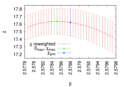
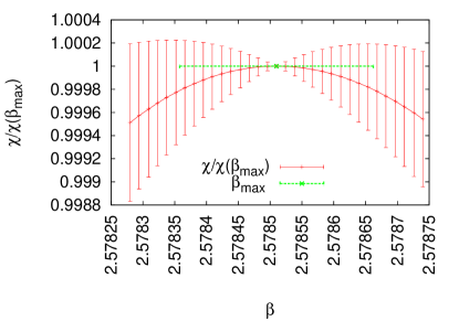
For $N_{\tau}=10$ and 12 the reweighting curve about the simulation point $\beta_{\rm sim}$ becomes rather flat within large error bars. See Fig. 1 for an example. Therefore, one may be amazed about the astonishingly accurate estimate of the maximum position $\beta_{\max}$. This is explained by the fact that all these error bars are strongly correlated, because they rely on reweighting of the same simulation. Dividing out the maximum value $\chi(\beta_{max})$ of the susceptibility in each jackknife bin, one is led to Fig. 2, which projects out the central part around the maximum of the previous figure and makes the (jackknife) error bars of the $\beta_{\max}$ estimate plausible.

The scaling analysis of the $N_{\tau}(\beta_{c})$ estimates of Tables 1 and 2 is performed in section V.

III Gradient scale

Before coming to our central issue of scale setting we define the SU(2) gradient flow, the observables used and sketch our generation of MCMC data.

III.1 Gradient flow

With initial condition $U_{\mu}(n,0)=U_{\mu}(n)$ the gradient flow is defined L10 by the evolution equation

$$\dot{U}_{\mu}(n,t) = -g_{0}^{2}\,\{\partial_{n,\mu}S[U(t)]\}\,U_{\mu}(n,t)\,.$$ (8)

Here the SU(2) link derivatives are given by

$$\partial_{n,\mu}f(U)=i\sum_{j=1}^{3}\sigma_{j}\left.\frac{d~{}}{ds}f(e^{isX^{j}}U)\right|_{s=0}\,,$$ (9)

where $\sigma_{j}$ are the Pauli matrices and

$$X^{j}(m,\nu)\ =\ \cases{\sigma^{j}\ {\rm if}\ (m,\nu)=(n,\mu)\,,\cr 0~{}~{}{\rm otherwise\,.}}$$ (10)

We use the notation $U_{\mu}^{\,{\mathchoice{\vbox{\hrule height=0.4pt\hbox{\vrule width=0.4pt,height=6.0pt\kern 6.0pt\vrule width=0.4pt} \hrule height=0.4pt}}{\vbox{\hrule height=0.4pt\hbox{\vrule width=0.4pt,height=6.0pt\kern 6.0pt\vrule width=0.4pt} \hrule height=0.4pt}}{\vbox{\hrule height=0.3pt\hbox{\vrule width=0.3pt,height=3.0pt\kern 3.0pt\vrule width=0.3pt} \hrule height=0.3pt}}{\vbox{\hrule height=0.3pt\hbox{\vrule width=0.3pt,height=3.0pt\kern 3.0pt\vrule width=0.3pt} \hrule height=0.3pt}}}}$ for the sum of plaquette matrices containing the link matrix $U_{\mu}$. With the definition of the staple matrix,

$$U^{\sqcup}_{\mu}(n) = \sum_{\nu\neq\mu}U_{\nu}(n)\,U_{\mu}(n+\hat{\nu})\,U^{\dagger}_{\nu}(n+\hat{\mu})$$

$$+ \sum_{\nu\neq\mu}U^{\dagger}_{\nu}(n-\hat{\nu})\,U_{\mu}(n-\hat{\nu})\,U_{\mu}(n-\hat{\nu}+\hat{\mu})\,,$$

this is

$$U_{\mu}^{\,{\mathchoice{\vbox{\hrule height=0.4pt\hbox{\vrule width=0.4pt,height=6.0pt\kern 6.0pt\vrule width=0.4pt} \hrule height=0.4pt}}{\vbox{\hrule height=0.4pt\hbox{\vrule width=0.4pt,height=6.0pt\kern 6.0pt\vrule width=0.4pt} \hrule height=0.4pt}}{\vbox{\hrule height=0.3pt\hbox{\vrule width=0.3pt,height=3.0pt\kern 3.0pt\vrule width=0.3pt} \hrule height=0.3pt}}{\vbox{\hrule height=0.3pt\hbox{\vrule width=0.3pt,height=3.0pt\kern 3.0pt\vrule width=0.3pt} \hrule height=0.3pt}}}}(n)=U_{\mu}(n)\,U^{\sqcup}_{\mu}(n)^{\dagger}\,.$$ (12)

For the SU(2) link derivative (9) one finds the simple equation

$$g_{0}^{2}\,\partial_{n,\mu}S(U)\ =\ \frac{1}{2}\left(U_{\mu}^{\,{\mathchoice{\vbox{\hrule height=0.4pt\hbox{\vrule width=0.4pt,height=6.0pt\kern 6.0pt\vrule width=0.4pt} \hrule height=0.4pt}}{\vbox{\hrule height=0.4pt\hbox{\vrule width=0.4pt,height=6.0pt\kern 6.0pt\vrule width=0.4pt} \hrule height=0.4pt}}{\vbox{\hrule height=0.3pt\hbox{\vrule width=0.3pt,height=3.0pt\kern 3.0pt\vrule width=0.3pt} \hrule height=0.3pt}}{\vbox{\hrule height=0.3pt\hbox{\vrule width=0.3pt,height=3.0pt\kern 3.0pt\vrule width=0.3pt} \hrule height=0.3pt}}}}(n)-U_{\mu}^{\,{\mathchoice{\vbox{\hrule height=0.4pt\hbox{\vrule width=0.4pt,height=6.0pt\kern 6.0pt\vrule width=0.4pt} \hrule height=0.4pt}}{\vbox{\hrule height=0.4pt\hbox{\vrule width=0.4pt,height=6.0pt\kern 6.0pt\vrule width=0.4pt} \hrule height=0.4pt}}{\vbox{\hrule height=0.3pt\hbox{\vrule width=0.3pt,height=3.0pt\kern 3.0pt\vrule width=0.3pt} \hrule height=0.3pt}}{\vbox{\hrule height=0.3pt\hbox{\vrule width=0.3pt,height=3.0pt\kern 3.0pt\vrule width=0.3pt} \hrule height=0.3pt}}}}(n)^{\dagger}\right)\,,$$ (13)

and we calculate the time evolution (8) using the Runge-Kutta scheme described in appendix C of L10 with

$$Z_{i}=\epsilon\,Z(W_{i})\,,~{}~{}Z(W_{i})=\frac{1}{2}\,\left(W_{i}-W_{i}^{\dagger}\right)\,,$$ (14)

$W_{0}=U_{\mu}(n,t)$ as starting values and $\epsilon=0.01$.

III.2 Observables

For the lattice expectation values of the time dependent plaquette matrices we use the parametrization

$$\left<U^{\,{\mathchoice{\vbox{\hrule height=0.4pt\hbox{\vrule width=0.4pt,height=6.0pt\kern 6.0pt\vrule width=0.4pt} \hrule height=0.4pt}}{\vbox{\hrule height=0.4pt\hbox{\vrule width=0.4pt,height=6.0pt\kern 6.0pt\vrule width=0.4pt} \hrule height=0.4pt}}{\vbox{\hrule height=0.3pt\hbox{\vrule width=0.3pt,height=3.0pt\kern 3.0pt\vrule width=0.3pt} \hrule height=0.3pt}}{\vbox{\hrule height=0.3pt\hbox{\vrule width=0.3pt,height=3.0pt\kern 3.0pt\vrule width=0.3pt} \hrule height=0.3pt}}}}(t)\right>_{L}\ =\ a_{0}(t)\,\sigma_{0}+i\,\sum_{i=1}^{3}a_{i}(t)\,\sigma_{i}\,,$$ (15)

where we suppress the $\mu\nu$ subscripts and $\sigma_{0}$ is the $2\times 2$ unit matrix, supplementing the Pauli matrices $\sigma_{j}$. As observables we use three definitions of the energy density: $E_{0}(t)$, $E_{1}(t)$ and $E_{4}(t)$. Up to a constant factor

$$E_{0}(t)\ =\ 2\,\left[1-a_{0}(t)\right]\,$$ (16)

is the usual Wilson action, i.e., becomes $\sim F_{\alpha\beta}F_{\alpha\beta}$ in the continuum limit. The definition

$$E_{1}(t)\ =\ \sum_{i=1}^{3}a_{i}(t)^{2}$$ (17)

has the same continuum limit as $E_{0}$. Finally, we denote by $E_{4}(t)$ Lüscher’s L10 energy density which averages over the four plaquettes attached to each site $n$ in a fixed $\mu\nu$, $\mu\neq\nu$ plane, i.e.,

$$E_{4}(t) = \sum_{i=1}^{3}b_{i}(t)^{2}\,,$$ (18)

$$b_{i}(t) = \frac{1}{4}\,\left(a_{i}^{ul}+a_{i}^{ur}+a_{i}^{dl}+a_{i}^{dr}\right),$$

where the superscripts of $a_{i}$ stand for up ($u$), left ($l$), right ($r$), and down ($d$) in a fixed $\mu\nu$ plane with respect to $n$ (drawn in Fig. 1 of L10 ). The functions

$$y_{i}(t)\ =\ t^{2}\,E_{i}(t)\,,~{}~{}(i=0,1,4)$$ (19)

are used to set the three gradient scales by choosing appropriate fixed values $y_{i}^{0}$ and iterating the time evolution (19) until

$$y_{i}^{0}\ =\ (t_{i}^{0})^{2}\,E_{i}(t_{i}^{0})$$ (20)

is reached. As function of $\beta$ the observable

$$s_{i}^{0}(\beta)\ =\ \sqrt{t_{i}^{0}(\beta)}$$ (21)

then scales like a length provided the following conditions are met:

1. Lattice sizes have to be chosen so that $N_{\min}\gg\sqrt{8}\,s_{i}^{0}$ holds, where $\sqrt{8}\,s_{i}^{0}$ is the smoothing range L10 and $N_{\min}=\min\{N_{i},i=1,2,3,4\}$ for simulations on a $N_{1}N_{2}N_{3}N_{4}$ lattice.

2. The values of $\beta$ have to be large enough to be in the SU(2) scaling region.

3. The values of $y_{i}^{0}$ have to be large enough so that $\sqrt{8}\,s_{i}^{0}\gg 1$ holds for the smallest used flow time.

III.3 Data generation and analysis

Our numerical results rely on MCMC simulations for the $\beta$ values and lattice sizes given in Table 3 and (identically) in subsequent tables. In each run $128=2^{7}$ configurations were generated and on each of them the gradient flow was performed. To optimize our use of computational resources, we followed the rule of B04 and allocated our CPU time in approximately equal parts to generation of configurations and to measurements (gradient flow). Subsequent configurations were separated by $2^{11}$ to $2^{13}$ MCOR sweeps where the increase from $2^{11}$ to larger numbers of MCOR sweeps is essentially enforced by the number of gradient sweeps needed to reach the $y^{0}_{i}$ target values. The dividing line from $2^{11}$ to $2^{12}$ sweeps is between $\beta=2.574$ and $\beta=2.62$, and from $2^{12}$ to $2^{13}$ between $\beta=2.67$ and $\beta=2.71$. We estimated integrated autocorrelation times $\tau_{\rm int}$ for the time series of 128 measured scale values and found all $\tau_{\rm int}$ compatible with 1 (in units of the number of sweeps between the configurations). So, the data are considered to be statistically independent. Error bars were calculated by the jackknife method with respect to the 128 configurations. Mostly, we used $N^{4}$ lattices with the exception of $24^{3}48$ and $32^{3}64$, which mirror lattices used in L10 . The scale estimates from these asymmetric lattices are consistent with those we obtained from $N^{4}$ lattices.

III.4 Scale setting

Table 3: Gradient length scale for its $y^{01}_{i}$ set (23).

$\beta$	Lattice	$L_{1}=s_{0}^{01}$	$L_{2}=s_{1}^{01}$	$L_{3}=s_{4}^{01}$
2.3	$8^{4}$	1.361  (13)	1.361  (13)	1.359  (15)
2.3	$12^{4}$	1.3538 (52)	1.3538 (50)	1.2955 (88)
2.3	$16^{4}$	1.3593 (28)	1.3589 (27)	1.2756 (75)
2.43	$12^{4}$	2.126  (20)	2.115  (20)	2.038  (20)
2.43	$16^{4}$	2.0961 (91)	2.0848 (90)	1.964  (14)
2.43	$24^{4}$	2.1066 (41)	2.0952 (40)	1.974  (11)
2.43	$28^{4}$	2.1023 (30)	2.0911 (30)	1.9666 (98)
2.51	$16^{4}$	2.730  (21)	2.715  (21)	2.603  (23)
2.51	$20^{4}$	2.766  (15)	2.750  (15)	2.585  (20)
2.51	$28^{4}$	2.7590 (73)	2.7428 (73)	2.570  (14)
2.574	$20^{4}$	3.389  (26)	3.369  (26)	3.166  (28)
2.574	$24^{4}$	3.395  (17)	3.374  (17)	3.175  (22)
2.574	$32^{4}$	3.406  (11)	3.385  (11)	3.193  (17)
2.574	$40^{4}$	3.4103 (72)	3.3896 (71)	3.149  (16)
2.62	$24^{4}$	3.993  (28)	3.968  (28)	3.711  (35)
2.62	$24^{3}48$	3.947  (22)	3.923  (21)	3.699  (26)
2.62	$28^{4}$	3.950  (20)	3.926  (20)	3.704  (24)
2.62	$40^{4}$	3.954  (10)	3.9293 (99)	3.672  (19)
2.67	$28^{4}$	4.680  (33)	4.651  (33)	4.350  (39)
2.67	$32^{4}$	4.651  (27)	4.622  (27)	4.350  (33)
2.67	$40^{4}$	4.622  (17)	4.593  (17)	4.297  (24)
2.71	$32^{4}$	5.217  (37)	5.185  (37)	4.867  (42)
2.71	$36^{4}$	5.252  (33)	5.220  (33)	4.852  (42)
2.71	$40^{4}$	5.199  (22)	5.167  (22)	4.817  (27)
2.751	$32^{3}64$	5.879  (35)	5.843  (34)	5.466  (39)
2.751	$36^{4}$	5.893  (38)	5.856  (38)	5.465  (48)
2.751	$40^{4}$	5.909  (34)	5.872  (34)	5.457  (41)
2.816	$44^{4}$	7.092  (48)	7.049  (47)	6.530  (54)
2.875	$52^{4}$	8.510  (64)	8.456  (65)	7.883  (68)

Table 4: Gradient length scale for its $y^{02}_{i}$ set (24).

$\beta$	Lattice	$L_{4}=s_{0}^{02}$	$L_{5}=s_{1}^{02}$	$L_{6}=s_{4}^{02}$
2.3	$8^{4}$	1.897  (24)	1.897  (24)	1.900 (25)
2.3	$12^{4}$	1.8905 (84)	1.8897 (83)	1.824 (12)
2.3	$16^{4}$	1.8963 (48)	1.8956 (48)	1.807 (11)
2.43	$12^{4}$	2.849  (34)	2.842  (33)	2.771 (34)
2.43	$16^{4}$	2.791  (15)	2.784  (15)	2.653 (20)
2.43	$24^{4}$	2.8044 (66)	2.7968 (65)	2.644 (15)
2.43	$28^{4}$	2.7994 (48)	2.7920 (47)	2.645 (13)
2.51	$16^{4}$	3.586  (34)	3.575  (34)	3.436 (34)
2.51	$20^{4}$	3.653  (25)	3.642  (25)	3.453 (29)
2.51	$28^{4}$	3.624  (12)	3.613  (12)	3.406 (19)
2.574	$20^{4}$	4.437  (39)	4.423  (39)	4.178 (44)
2.574	$24^{4}$	4.429  (26)	4.415  (26)	4.171 (29)
2.574	$32^{4}$	4.454  (15)	4.440  (15)	4.219 (22)
2.574	$40^{4}$	4.458  (12)	4.444  (11)	4.175 (21)
2.62	$24^{4}$	5.252  (46)	5.233  (45)	4.916 (49)
2.62	$24^{3}48$	5.135  (33)	5.119  (33)	4.868 (38)
2.62	$28^{4}$	5.145  (30)	5.129  (30)	4.849 (32)
2.62	$40^{4}$	5.156  (16)	5.140  (16)	4.827 (26)
2.67	$28^{4}$	6.131  (53)	6.110  (53)	5.740 (60)
2.67	$32^{4}$	6.057  (40)	6.038  (40)	5.719 (46)
2.67	$40^{4}$	6.020  (27)	6.000  (27)	5.645 (32)
2.71	$32^{4}$	6.776  (55)	6.754  (55)	6.357 (56)
2.71	$36^{4}$	6.831  (50)	6.809  (50)	6.401 (57)
2.71	$40^{4}$	6.773  (32)	6.751  (32)	6.334 (39)
2.751	$32^{3}64$	7.642  (51)	7.617  (51)	7.179 (57)
2.751	$36^{4}$	7.659  (60)	7.633  (59)	7.161 (68)
2.751	$40^{4}$	7.694  (50)	7.668  (50)	7.211 (59)

Figure 3: Gradient flows $y_{i}(t)$ for the energy densities $E_{0}$, $E_{1}$ and $E_{4}$ at $\beta=2.3$ on an $8^{4}$ lattice ($t$ on lower abscissa) and at $\beta=2.574$ on a $40^{4}$ lattice ($t$ on upper abscissa). The up-down order in the legend agrees on the right-hand side with that of the curves.

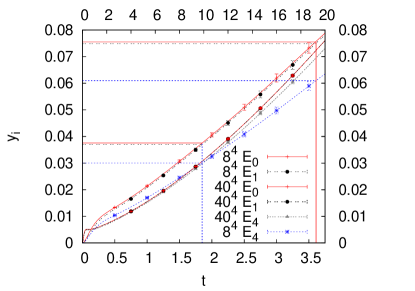
From estimates of the deconfinement $\beta_{c}(N_{\tau})$ values we know that it only makes sense to investigate SU(2) scaling for $\beta\geq 2.29$, $N_{\tau}\geq 4$. The smallest $N_{s}^{3}\,4$ lattice size that can be used for the $N_{\tau}=4$, $N_{s}\to\infty$ finite size extrapolation is given by $N_{s}=8$. Therefore, it is natural to start our gradient flow simulations at $\beta=2.3$ on an $8^{4}$ lattice and to work from there up to larger $\beta$ values and lattice sizes. It is of interest to control scaling violations at the lower end of the scaling region, because simulations there are less expensive than at larger $\beta$.

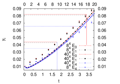
The upper two curves (red, black online) and the, ultimately, lowest (blue online) curve of Fig. 3 show $y_{i}(t)$, ($i=0,1,4$) from simulations on an $8^{4}$ lattice ($t$ on the lower abscissa). While the plots corresponding to $E_{0}$ and $E_{1}$ fall practically on top of one another, they deviate from the plot for $E_{4}$. This is due to finite lattice size corrections as well as scaling corrections in $\beta$. These corrections are much smaller for the other three curves which are from simulations at $\beta=2.574$ on a $40^{4}$ lattice. The corresponding $t$ values are on the upper abscissa and chosen so that the largest $y$-values reached agree approximately with those from the $8^{4}$ lattice.

Figure 4: Gradient flow ratios as functions of $y$. Outer curves: $s_{i}(12,2.43)/s_{i}(8,2.3)$. Inner curves: $s_{i}(24,2.43)/s_{i}(16,2.3)$.

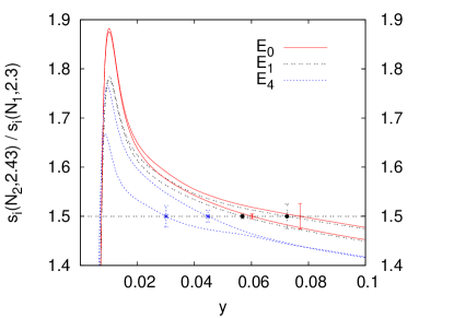
The question is this: How does one pick a set of $y_{i}^{0}$ values that defines suitable $s^{0}_{i}$ scales according to Eqs. (20) and (21)? To minimize CPU time, one likes to keep the lattice size and $s_{0}^{i}$ as small as possible. On the other hand, smaller $s_{0}^{i}$ values imply larger discretization (finite lattice spacing) corrections and too small lattices imply finite size corrections. It is at this point that one encounters considerable ambiguities in the definition of gradient (and similarly cooling) scales.

In our context it is natural to define $y_{i}^{0}$ values so that our initial estimates from the $s^{0}_{i}$ scales are consistent with those from low $\beta_{c}(N_{\tau}$) values. Lowest reasonable starting values for $\beta$, corresponding approximately to the $\beta_{c}(4)$ and $\beta_{c}(6)$ estimates of Table 1, are $\beta_{1}=2.3$ and $\beta_{2}=2.43$. In Fig. 4 we plot ratio functions

$$\frac{s_{i}(N_{2},\beta_{2}=2.43)}{s_{i}(N_{1},\beta_{1}=2.3)}\,(y)$$ (22)

for $(N_{2},N_{1})=(12,8)$ and $(24,16)$. On the 1.5 line the outer curves correspond to $(12,8)$ and the inner curves (using the same colors) to $(24,16)$. To prevent the figure from becoming too convoluted, error bars are only given on this line. As one expects from Fig. 3, the $y$ values of the $E_{4}$ crossing points are apart from those of $E_{0}$ and $E_{1}$. The difference is considerably reduced when finite lattice size corrections are remediated by moving to (24,16) lattices. The remaining difference should mainly be attributed to corrections in $\beta$ (i.e., finite lattice spacing corrections).

One may have expected a plateau in the neighborhood of the 1.5 line, indicating that the ratios do not depend on the precise choice of the $y_{i}^{0}$ target values. Instead, without using the deconfinement result as input, another uncertainty in the choice of the $y_{i}^{0}$ target values would exist.

In the following we use the outer values of Fig. 4 and explore whether their differences result in seriously distinct scaling behavior. Starting off with $\beta=2.3$, we are exploring two gradient scales:

1. We define the $y_{i}^{01}$ scale so that the $E_{4}$ observable delivers $s_{4}^{01}(12,2.43)/s_{4}^{01}(8,2.3)=1.5$.

2. We define the $y_{i}^{02}$ scale so that for the $E_{i}$, $i=0,1$, observables $s_{i}^{02}(12,2.43)/s_{i}^{02}(8,2.3)=1.5$ holds.

For the first case we find $y_{4}^{01}=0.030$ from Fig. 4. Using $y_{4}(t)$ depicted in Fig. 3, $y_{4}^{01}=0.030$ converts into the $t$ value $t^{01}=1.85$ for the flow time, as indicated by a vertical line. Its intersections with the $y_{i}(t)$ functions define our first set of $y_{i}^{0}$ target values

$$y^{01}_{0}=0.0376\,,~{}~{}~{}y^{01}_{1}=0.0370\,,~{}~{}~{}y^{01}_{4}=0.030\,.$$ (23)

Similarly, our second set of $y_{i}^{0}$ values is derived from $t^{02}=3.61$, which is the average value of $t$ of the relevant crossing points of the $E_{0}$ and $E_{1}$ observables. This $t^{02}$ value is also shown as a vertical line in Fig. 3 and leads to

$$y^{02}_{0}=0.0755\,,~{}~{}~{}y^{02}_{1}=0.0748\,,~{}~{}~{}y^{02}_{4}=0.061\,.$$ (24)

Length scale values

$$s_{i}^{0j}(\beta)\ =\ \sqrt{t_{i}^{0j}(\beta)}\,,~{}~{}i=0,1,4,~{}~{}j=1,2$$ (25)

are obtained when the gradient flow hits the corresponding $y_{i}^{0j}$ definitions of Eqs. (23) or (24). Our MCMC estimates for them are reported in Tables 3 and 4. For later convenience we label the length scales by $L_{1}$ to $L_{6}$ as defined in the first row of the tables. We are led to $\sqrt{8\,t^{01}}\approx 3.85$ and $\sqrt{8\,t^{02}}\approx 5.37$ as our smallest values for the smoothing range. This is below and above the starting value $\sqrt{8\,t^{0}}\approx 4.77$ of Ref. L10 taken at $\beta=5.96$ in the SU(3) scaling region. Comparing the SU(3) deconfinement transition values $\beta_{c}$ for $N_{\tau}=4$, 6, 8 (see, e.g., Ref. Fr15 ) with those for SU(2) and performing interpolations of the $\beta_{c}$ values, this corresponds roughly to $\beta=2.46$ for SU(2), where our lower smoothing range has increased to at least 6.64. So, our lower smoothing range is also effectively larger than the one of L10 .

For each $\beta$ value several lattice sizes are listed in Tables 3 and 4 to control finite size corrections. In most cases they are sufficiently weak to be swallowed by the statistical error bars. Exceptions are the ${s}_{4}^{0j}$ estimates on $8^{4}$ and $12^{4}$ lattices at $\beta=2.3$ and 2.43, which appear to be too small to accommodate $E_{4}$. Up to $\beta=2.751$ lattices of size $40^{4}$ appear to be large enough so that finite size corrections can be neglected. Larger lattices would just increase statistics due to self-averaging. For our largest lattices with $\beta=2.816$ and 2.875 the gradient flow was designed too short to reach the $y_{i}^{02}$ targets (24).

IV Cooling scale

Figure 5: Cooling flows $y_{i}(t)$ for the energy densities $E_{0}$, $E_{1}$ and $E_{4}$ at $\beta=2.3$ on an $8^{4}$ lattice ($t$ on lower abscissa) and at $\beta=2.574$ on a $40^{4}$ lattice ($t$ on upper abscissa).

Table 5: Cooling length scale for its $y^{01}_{i}$ set (29).

$\beta$	Lattice	$L_{7}=s_{0}^{01}$	$L_{8}=s_{1}^{01}$	$L_{9}=s_{4}^{01}$
2.3	$8^{4}$	1.342  (12)	1.337  (12)	1.342  (14)
2.3	$12^{4}$	1.3391( 47)	1.3343 (45)	1.2730 (85)
2.3	$16^{4}$	1.3433 (24)	1.3385 (23)	1.2575 (74)
2.43	$12^{4}$	2.111  (19)	2.092  (18)	2.013  (20)
2.43	$16^{4}$	2.0837 (90)	2.0653 (90)	1.951  (13)
2.43	$24^{4}$	2.0929 (38)	2.0744 (38)	1.947  (11)
2.43	$28^{4}$	2.0892 (28)	2.0707 (28)	1.9446 (95)
2.51	$16^{4}$	2.728  (19)	2.703  (19)	2.587  (23)
2.51	$20^{4}$	2.753  (14)	2.727  (14)	2.567  (20)
2.51	$28^{4}$	2.7522 (68)	2.7267 (66)	2.548  (15)
2.574	$20^{4}$	3.396  (25)	3.365  (24)	3.157  (26)
2.574	$24^{4}$	3.389  (16)	3.357  (16)	3.155  (22)
2.574	$32^{4}$	3.4001 (97)	3.3686 (95)	3.153  (17)
2.574	$40^{4}$	3.4048 (69)	3.3730 (67)	3.137  (17)
2.62	$24^{4}$	3.988  (26)	3.949  (26)	3.717  (32)
2.62	$24^{3}48$	3.949  (20)	3.912  (19)	3.688  (25)
2.62	$28^{4}$	3.952  (19)	3.915  (19)	3.680  (23)
2.62	$40^{4}$	3.9509 (95)	3.9137 (93)	3.645  (22)
2.67	$28^{4}$	4.676  (32)	4.631  (31)	4.314  (39)
2.67	$32^{4}$	4.644  (27)	4.600  (26)	4.282  (31)
2.67	$40^{4}$	4.618  (17)	4.574  (16)	4.298  (26)
2.71	$32^{4}$	5.216  (36)	5.167  (35)	4.833  (41)
2.71	$36^{4}$	5.256  (31)	5.207  (31)	4.803  (42)
2.71	$40^{4}$	5.203  (21)	5.154  (21)	4.794  (28)
2.751	$32^{3}64$	5.874  (32)	5.819  (32)	5.437  (37)
2.751	$36^{4}$	5.892  (36)	5.836  (35)	5.478  (49)
2.751	$40^{4}$	5.913  (32)	5.857  (32)	5.434  (40)
2.816	$44^{4}$	7.105  (45)	7.039  (45)	6.511  (55)
2.875	$52^{4}$	8.514  (60)	8.433  (59)	7.825  (68)

Table 6: Cooling length scale for its $y^{02}_{i}$ set (30).

$\beta$	Lattice	$L_{10}=s_{0}^{02}$	$L_{11}=s_{1}^{02}$	$L_{12}=s_{4}^{02}$
2.3	$8^{4}$	1.846  (22)	1.844  (22)	1.843 (22)
2.3	$12^{4}$	1.8241 (74)	1.8217 (72)	1.743 (12)
2.3	$16^{4}$	1.8307 (39)	1.8282 (39)	1.728 (10)
2.43	$12^{4}$	2.769  (29)	2.759  (29)	2.669 (32)
2.43	$16^{4}$	2.725  (14)	2.715  (14)	2.572 (18)
2.43	$24^{4}$	2.7395 (57)	2.7287 (57)	2.561 (14)
2.43	$28^{4}$	2.7317 (43)	2.7212 (42)	2.565 (12)
2.51	$16^{4}$	3.531  (30)	3.516  (30)	3.370 (31)
2.51	$20^{4}$	3.571  (23)	3.555  (23)	3.359 (27)
2.51	$28^{4}$	3.552  (10)	3.5371 (99)	3.315 (18)
2.574	$20^{4}$	4.356  (37)	4.337  (37)	4.084 (38)
2.574	$24^{4}$	4.352  (24)	4.333  (24)	4.080 (29)
2.574	$32^{4}$	4.374  (14)	4.355  (14)	4.100 (21)
2.574	$40^{4}$	4.377  (11)	4.358  (10)	4.074 (20)
2.62	$24^{4}$	5.157  (40)	5.133  (39)	4.836 (44)
2.62	$24^{3}48$	5.070  (30)	5.047  (29)	4.788 (34)
2.62	$28^{4}$	5.059  (28)	5.037  (28)	4.751 (30)
2.62	$40^{4}$	5.068  (15)	5.045  (15)	4.725 (26)
2.67	$28^{4}$	6.021  (46)	5.993  (46)	5.603 (58)
2.67	$32^{4}$	5.950  (38)	5.923  (38)	5.532 (42)
2.67	$40^{4}$	5.910  (25)	5.884  (25)	5.536 (33)
2.71	$32^{4}$	6.656  (51)	6.626  (51)	6.208 (55)
2.71	$36^{4}$	6.724  (48)	6.692  (48)	6.223 (58)
2.71	$40^{4}$	6.656  (31)	6.626  (30)	6.188 (38)
2.751	$32^{3}64$	7.515  (49)	7.481  (48)	7.010 (52)
2.751	$36^{4}$	7.531  (53)	7.497  (53)	7.033 (66)
2.751	$40^{4}$	7.576  (46)	7.541  (46)	7.038 (54)
2.816	$44^{4}$	9.056  (65)	9.015  (64)	8.349 (73)
2.875	$52^{4}$	10.879  (87)	10.830  (86)	10.122 (92)

The cooling method was introduced in Ref. B81 in the context of investigating the topological charge of the 2D O(3) sigma model. It has since then found many applications. For a review see N99 . A SU(2) cooling update maps a link matrix

$$U_{\mu}(n)\ \to\ U^{\prime}_{\mu}(n)\,,$$ (26)

so that $U^{\prime}_{\mu}(n)$ maximizes the local contribution to the action. This is achieved by

$$U^{\prime}_{\mu}(n)\ =\ U^{\sqcup}_{\mu}(n)/{\rm det}|U^{\sqcup}_{\mu}(n)|\,,$$ (27)

where $U^{\sqcup}_{\mu}(n)$ is the staple matrix (III.1), which for SU(2) agrees up to the determinant factor with a SU(2) matrix.

Our cooling sweeps are performed in the same systematic order as our MCMC sweeps. Bonati and D’Elia BD14 outlined that $n_{c}$ cooling sweeps correspond to a gradient flow time

$$t_{c}\ =\ n_{c}/3\,.$$ (28)

As we use $\epsilon=0.01$ in our gradient flow steps, one cooling sweep corresponds to $33.\overline{3}$ gradient sweeps. On top of this (because of the Runge-Kutta), one gradient sweep is more CPU time demanding than one cooling sweep, so that the computational efficiency is improved by at least a factor of 34. A priori it is not obvious that many small gradient flow steps can be replaced by a large cooling step without losing accuracy of scale setting. A posteriori our results support that such a replacement is permissible.

Figure 5 is the analogue of Fig. 3. Due to the large cooling steps, gaps between them are clearly visible. They also exist in Fig. 3, but are there too small to be noticeable. Using linear interpolations, the crossing points of the ratio functions (22) determine initial scales for the cooling flow in precisely the same way as explained for the gradient flow. The values are summarized by the equations $t^{01}=1.80$, $t^{02}=3.40$,

$$y^{01}_{0} = 0.0440\,,~{}~{}y^{01}_{1}\ =\ 0.0430\,,~{}~{}y^{01}_{4}\ =\ 0.0350\,,~{}~{}~{}~{}$$ (29)

$$y^{02}_{0} = 0.0822\,,~{}~{}y^{02}_{1}\ =\ 0.0812\,,~{}~{}y^{02}_{4}\ =\ 0.0656\,.~{}~{}~{}~{}$$ (30)

The cooling scale ${s}_{i}^{0j}(\beta)$ values (25) are collected in Tables 5 and 6 for the same lattices and $\beta$ values as used for the gradient flow. For the analysis in the next section these length scales are labeled by $L_{7}$ to $L_{12}$. A detailed comparison of the scaling behavior of the deconfinement, gradient and cooling scales follows in the next section.

V Scaling and asymptotic scaling

In this section we analyze scaling and asymptotic scaling for 13 length scales

$$L_{k}\,,~{}~{}~{}(k=0,\dots,12)\,$$ (31)

defined as follows: The deconfining scale $L_{0}=N_{\tau}(\beta_{c})$ (4), six gradient, $L_{1},\dots,L_{6}$, and six cooling, $L_{7},\dots,L_{12}$, length scales. First, we consider ${\cal O}(a^{2})$ scaling corrections for length ratios in the usual way (e.g., L10 ). Then, we incorporate asymptotic scaling behavior along the lines of Ref. A97 ; B15 and show how this can be done in a way consistent with ${\cal O}(a^{2})$ scaling corrections.

V.1 Scaling

Table 7: Estimates of $r_{ij}$ ratios defined by Eq. (33).

$i\,\backslash\,j$	$L_{1}$	$L_{4}$	$L_{7}$	$L_{10}$
$L_{0}$	2.8896 (71)	2.2290 (46)	2.8855 (68)	2.2618 (42)
$L_{1}$	$-$	0.77382 (61)	0.99845 (38)	0.78433 (43)
$L_{3}$	0.9250 (19)	0.7163 (17)	0.9241 (19)	0.7264 (16)
$L_{4}$	1.2943 (11)	$-$	1.29135 (99)	1.01520 (49)
$L_{6}$	1.2090 (26)	0.9346 (20)	1.2081 (27)	0.9490 (21)
$L_{7}$	1.00156 (38)	0.77398 (79)	$-$	0.78570 (50)
$L_{9}$	0.9222 (21)	0.7141 (19)	0.9213 (20)	0.7243 (17)
$L_{10}$	1.27509 (70)	0.98508 (47)	1.27300 (80)	$-$
$L_{12}$	1.1835 (24)	0.9164 (21)	1.1825 (24)	0.9292 (19)

To compare mass or length scales it is customary to fit ratios to the linear form

$$R_{ij}=\frac{L_{i}}{L_{j}}=r_{ijk}+c_{ijk}\,\left(\frac{a}{l_{k}}\right)^{2},~{}~{}l_{k}=a\,L_{k}\,,$$ (32)

where $a$ is the lattice spacing, $l_{k}$ the length scale in physical units and $r_{ijk}$, $c_{ijk}$ are fit parameters of which the $r_{ijk}$ estimate the continuum limits and $c_{ijk}$ the leading order corrections. We report in Table 7 continuum estimates $r_{ij}$ for the subset

$$R_{ij}=r_{ij}\!+\!c_{ij}\,\left(\frac{a}{l_{j}}\right)^{2}=r_{ij}\!+\!c_{ij}\,\left(\frac{1}{L_{j}}\right)^{2}$$ (33)

with $i=0,1,3,4,6,7,9,10,12$ and $j=1,4,7,10$. For $i\geq 1$ gradient and cooling scale fits, we use at each $\beta$ value our largest lattice and $R_{ij}$ error bars that rely on jackknife binning. In the case of the $L_{0}$ deconfinement scale, error propagation is used, where the values of the gradient and cooling scales at the $\beta_{c}$ values are obtained by interpolating via an asymptotic scaling fit performed in the next subsection.

The scales $L_{2}$, $L_{5}$, $L_{8}$ and $L_{11}$ are omitted from the table, because they rely on the $E_{1}$ energy definition, which agrees for practical purposes with $E_{0}$. For instance, $r_{11,10}=0.995397\,(24)$, where the error bar is very small due to correlations between the $E_{0}$ and $E_{1}$ energy densities. Data points from $\beta=2.3$ are eliminated from the fits for $q$ values smaller than $0.05$. After applying this cut, $q$ was in the range 0.11 to 0.98.

Figure 6: Scaling corrections of order $a^{2}$ for ratios $L_{i}/L_{10}$. Here and in the next figures some data are slightly shifted for better visibility. To label all fits, some labels are attached to the lines and others put into the legend. The up-down order in the legend mirrors the up-down order in the plot.

Figure 7: Enlargement of the continuum approach of Fig. 6 for the $E_{0}$, the $L_{11}$ and the deconfinement scales.

Figure 8: Enlargement of the continuum approach of Fig. 6 for the $E_{4}$ scales.

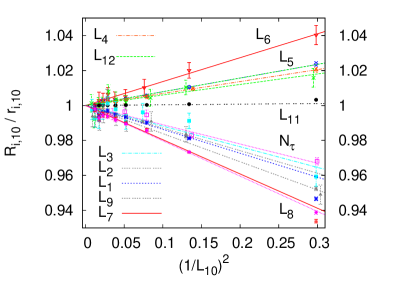
To compare scaling corrections we divide the $R_{ij}$ data by their continuum limits $r_{ij}$ and choose as reference scale $j=10$ by reasons to be explained. A selection of the thus resulting fits is plotted in Fig. 6.

The fit for the deconfinement scale $N_{\tau}$ relies on the five $\beta_{c}$ data points of Tables 1, 2 and has a goodness of fit $q=0.25$. The $q<0.05$ cut was applied to the fits involving $L_{11}$, $L_{2}$, $L_{1}$ and $L_{7}$. For them deviations of the $\beta=2.3$ data points from the fit lines are clearly visible in Fig. 6 at $(1/L_{10})^{2}\approx 0.3$. The remaining seven fits include their $\beta=2.3$ data points.

Essentially, the $L_{11}/L_{10}$ fit takes on the constant value 1. Similarly, $E_{0}$, $E_{1}$ pairs stay together for the other scales. Generally, we notice that gradient and cooling scales that use the same energy observable and target value $y_{i}^{01}$ or $y_{i}^{02}$ stay closer together than gradient scales using different energy observables and target values or cooling scales using different energy observables and target values. The ratios of Table 7 show the same pattern. So, it appears perfectly legitimate to use cooling instead of gradient scales. We opted for $L_{10}$ as reference scale, because it centers rather nicely with respect to the other scales. At $(1/L_{10})^{2}\approx 0.3$ in Fig. 6 we read off scaling violations of about 10%, i.e., 0.94 to 1.04 for $R_{i,10}/r_{i,10}$. That is larger than the 5% reported by Lüscher L10 in his Fig. 3 for SU(3) at $\beta=5.96$. As outlined, this corresponds to $\beta\approx 2.46$ for SU(2), which translates into $(1/L_{10})^{2}\approx 0.11$. In Fig. 6 this is slightly left of the column of data at $(1/L_{10})^{2}\approx 0.13$ for which we find the range $0.97<R_{i,10}/r_{i,10}<1.02$, i.e., scaling violations are down to less than 5%.

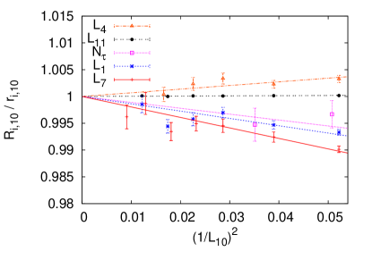
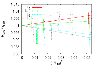
A problem with plots like Fig. 6 is that data from large lattices (close to the continuum limit) accumulate in a small region, which is here below $(1/L_{10})^{2}<0.05$. It is enlarged in Figs. 7 and 8. In Fig. 8 the length scales based on the $E_{4}$ energy are plotted and seen to exhibit considerably larger error bars than the energy scales plotted in Fig. 7. With no particular advantages to offset this lack of accuracy of the $E_{4}$ scales, all arguments converge in favor of using an $E_{0}$ cooling scale.

V.2 Asymptotic scaling

For large $\beta$ the scaling of any mass $m$ in pure SU(N) LGT is determined by the asymptotic scaling function

$$a\,m\ =\ {\rm const}\,f_{as}(\beta)\,,$$ (34)

$$f_{as}(\beta)\ =\ \alpha\,a\Lambda_{L}=\alpha\,\left(b_{0}\,\frac{2N}{\beta}\right)^{-b_{1}/2b^{2}_{0}}$$

$$\times \exp\left(-\frac{\beta}{4N\,b_{0}}\right)\,\left[1+\sum_{j=1}^{\infty}q_{j}\,\left(\frac{2N}{\beta}\right)^{j}\right]\,,$$

where $a$ is the lattice spacing, $b_{0}=11\,N/(48\pi^{2})$ and $b_{1}=(34/3)\,N^{2}/(16\pi^{2})^{2}$ are, respectively, the universal 1-loop Gr73 ; Po73 and 2-loop Jo74 ; Ca74 asymptotic scaling coefficients. Universal means that all renormalization schemes lead to the same $b_{0}$ and $b_{1}$ values. Non-universal perturbative corrections are given by the $q_{j}$ coefficients in the bracket. Computing up to 3-loops, Allés et al. AF97 calculated $q_{1}$ for SU(N) LGT and

$$q_{1}\ =\ 0.08324~{}~{}{\rm for\ SU(2)}\,.$$ (35)

Further, we introduce the factor $\alpha$ to enforce for SU(2) the convenient normalization

$$f_{as}(2.3)\ =\ 1\,.$$ (36)

Higher orders corrections in the lattice spacing $a$ are reflected by terms of the form

$$(\alpha\,a\Lambda_{L})^{i}=[f_{\rm as}(\beta)]^{i}\,,~{}~{}(i=2,3,\dots)\ .$$ (37)

Following Allton A97 in the version of B15 we arrive at the expansions

$$L_{k}=\frac{c_{k}}{f_{as}(\beta)}\,\left(1+\sum_{i=1}^{\infty}a_{k}^{i}\,[f_{as}(\beta)]^{i}\right)$$ (38)

for our length scales, where $c_{k}$ and the $a^{i}_{k}$ are parameters that have to be calculated. In practice we have to truncate the series (38) as well as the definition (34) of $f_{as}(\beta)$. Defining

$$f^{0}_{as}(\beta) = \alpha^{0}\,\left(b_{0}\,\frac{2N}{\beta}\right)^{-b_{1}/2b^{2}_{0}}\exp\left(-\frac{\beta}{4N\,b_{0}}\right)\,,~{}~{}~{}$$ (39)

$$f^{1}_{as}(\beta) = \left(\frac{\alpha^{1}}{\alpha^{0}}\right)\,f^{0}_{as}(\beta)\,\left(1+\frac{4\,q_{1}}{\beta}\right)\,,$$ (40)

we have $f^{m}_{as}$ with $m=0,1$ at our disposal, where the coefficients $\alpha^{m}$ are defined to enforce as in (36) the normalizations $f^{m}_{as}(2.3)=1$. Truncating the sum (38) by fixed $n$, we end up with 26 fits ($k=0,\dots,12$), ($m=0,1$):

$$L_{k}^{m,n}=\frac{c_{k}^{m,n}}{f^{m}_{as}(\beta)}\,\left(1+\sum_{i=1}^{n}a_{k}^{m,i}\,[f^{m}_{as}(\beta)]^{i}\right)\,,$$ (41)

where the index $n$ of $a_{k}^{m,i}$ is suppressed. Due to the truncation of $f_{as}$ there are perturbative corrections in $1/\beta$ when ratios are taken with respect to the (inverse) lambda lattice scale, i.e.,

$$L_{k}^{m,n}\,\alpha^{m}\,a\Lambda_{L}=c_{k}^{m,n}+{\rm perturbative\ corrections}$$ (42)

describes asymptotic scaling. Corrections to ratios of two length scales are exponentially small in $\beta$, i.e.,

$$\frac{L_{k_{1}}^{m,n_{1}}}{L_{k_{2}}^{m,n_{2}}}=\frac{c_{k_{1}}^{m,n_{1}}}{c_{k_{2}}^{m,n_{2}}}+{\rm non\!\!-\!\!perturbative\ corrections}\$$ (43)

holds. However, due to the $a^{m,1}_{k}$ term in (41) corrections would in general be of order $a$ in the lattice spacing and not of order $a^{2}$ as in (33). In B15 this problem was avoided by combining several scales into one fit. This is only possible when their relative scaling violations are so weak that they become invisible within statistical errors. The solution which we propose here is to fit all $k=0,1,\dots,12$ scales with identical $a^{m,1}_{k}$ coefficients so that the non-perturbative corrections (43) become ${\cal O}(a^{2})$.

Table 8: Asymptotic scaling fits of normalization constants and goodness of fit $q$.

$k$	$c_{k}^{1,3}$		$c_{k}^{0,4}$	$q$	$c_{k}^{1,4}$	$q$
0	6.6682 (56)	0.00	6.114 (29)	0.71	5.892 (27)	0.68
	$c_{k}^{1,2}$		$c_{k}^{0,3}$		$c_{k}^{1,3}$
1	2.2481 (32)	0.04	2.1937 (64)	0.91	2.1083 (61)	0.91
2	2.2311 (32)	0.03	2.1812 (64)	0.92	2.0961 (60)	0.92
3	2.0743 (56)	0.17	2.022  (11)	0.66	1.9432 (98)	0.67
4	2.8945 (54)	0.08	2.846  (11)	0.98	2.735  (11)	0.98
5	2.8835 (53)	0.04	2.837  (11)	0.98	2.727  (11)	0.98
6	2.7068 (85)	0.95	2.658  (18)	0.95	2.555  (17)	0.95
7	2.2498 (30)	0.02	2.1996 (61)	0.93	2.1138 (57)	0.94
8	2.2254 (30)	0.01	2.1807 (60)	0.92	2.0956 (57)	0.93
9	2.0664 (58)	0.16	2.018  (11)	0.69	1.9397 (99)	0.69
10	2.8501 (46)	0.02	2.8037 (91)	0.89	2.6942 (86)	0.89
11	2.8357 (45)	0.01	2.7914 (89)	0.88	2.6824 (85)	0.89
12	2.6485 (74)	0.26	2.599  (14)	0.52	2.498  (13)	0.52
	$a_{k}^{1,1}=-0.6209$		$a_{k}^{0,1}=-0.38157$		$a_{k}^{1,1}=-0.32536$

Estimates of normalization constants for asymptotic scaling fits are collected in Table 8. As before, the gradient and cooling scale fits use our largest lattice at each $\beta$ value. The last row of the table gives the $a_{k}^{m,1}$ values taken for all fits of their respective columns. Using the $E_{0}$ and $E_{4}$ scales these values were determined by the maximum likelihood method ($E_{1}$ scales are left out because they would in essence amplify weights of the $E_{0}$ scales). On a technical note, we remark that we eliminate the normalization constants $c_{k}^{m,n}$ from the search for the $\chi^{2}$ minimum by treating them as functions of the $a_{k}^{m,i}$ parameters B16 . This stabilizes the search considerably, for which we used the Levenberg-Marquardt approach (e.g., B04 ).

Fitting the gradient and cooling scales ($k\geq 1$) with only one additional parameter, $a_{k}^{1,2}$, the normalization constants $c_{k}^{1,2}$ of column two are obtained. Most $q$ values of these fits are too low. So, we decided to allow for one more fit parameter, $a_{k}^{m,3}$. The results are shown in columns four and six (using $f_{as}^{m}$ with $m=0,1$). Now, the $q$ values for these fits would be too good to be true if they were statistically independent. As they all rely on the same data set correlations can explain that a whole series of fits exhibits $q>0.5$, mostly close to 0.9. Notably, consistent fits due to adding the $a_{k}^{m,3}$ parameters come at the price of about doubled error bars compared to those of column two.

It is possible to include the deconfinement length scale into these fits with fixed $a_{k}^{m,1}$ and the results are given in the second row of Table 8. Despite the small number of only five data points (Tables 1 and 2) one needs one more parameter, $a_{0}^{m,4}$, to get acceptable $q$ values. This is accompanied by some instability discussed at the end of this section.

Using the $f^{1}_{as}$ instead of the $f^{0}_{as}$ asymptotic scaling function decreases all $c_{k}$ values by slightly less than 4%. More prominent is the decrease between 6.7% to 9% from column two to column six, which comes from allowing one more free parameter. Together we take this as an indication that remaining systematic errors may well reach 10%.

Figure 9: Asymptotic scaling.

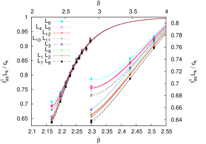
Dividing out the asymptotic scaling behavior $c_{k}^{1,n}/f^{1}_{as}(\beta)$, we plot in Fig. 9 the resulting fits $f^{1}_{as}\,L_{k}^{1,3}/c_{k}^{1,3}$ ($k\geq 1$) for column six of Table 8. For the curves on the left the abscissa is on top of the figure and the ordinate on the left. At $\beta=4$ all fits have almost reached the asymptotic value 1. The lower abscissa and the right ordinate apply to the right part of Fig. 9, which enlarges the range of our initial three $\beta$ values. At $\beta=2.3$ asymptotic scaling violations are seen to range from 28% to 37%. The relative differences reach only $0.72/0.63\approx 1.14$, consistent with the ratio $1.04/0.93\approx 1.12$ observed at $(1/L_{10})^{2}=0.3$ in Fig. 6.

Let us turn to the scaling behavior of ratios. Except for the deconfinement length scale $L_{0}$, which is statistically independent from the other scales, we cannot use error propagation. Instead, we calculate the $R_{ij}$ ratios (33) for jackknife bins built from the individual gradient or cooling flow runs (using jackknife bins of the asymptotic scaling fits of Table 8 has the problem that these fits have larger fluctuations than the $R_{ij}$ ratios).

Table 9: Estimates of $r_{ij}$ ratios from scaling fits of jackknifed $R_{ij}$ data.

$i\,\backslash\,j$	$L_{1}$	$L_{4}$	$L_{7}$	$L_{10}$
$L_{0}$ (as)	2.795 (16)	2.154 (14)	2.787 (15)	2.187 (13)
$L_{0}$	*2.914 (15)	2.2393 (52)	*2.903 (14)	2.2692 (48)
$L_{1}$	$-$	*0.7703 (12)	0.99808 (34)	*0.78185 (77)
$L_{3}$	0.9240 (20)	0.7187 (19)	0.9221 (20)	0.7275 (17)
$L_{4}$	*1.2996 (21)	$-$	*1.2957 (27)	1.01373 (57)
$L_{6}$	1.2000 (31)	0.9334 (23)	1.1972 (32)	0.9465 (24)
$L_{7}$	1.00188 (34)	*0.7728 (16)	$-$	*0.78419 (88)
$L_{9}$	0.9214 (22)	0.7171 (21)	0.9197 (22)	0.7255 (18)
$L_{10}$	*1.2795 (13)	0.98638 (55)	*1.2760 (15)	$-$
$L_{12}$	1.1786 (26)	0.9167 (24)	1.1760 (26)	0.9283 (20)

For $m=1$ results are collected in Table 9. With exception of the $L_{0}$ (as) row (to be discussed) all fits use

$$a_{k}^{1,1}\ =\ 0$$ (44)

to reflect that the leading scaling corrections for mass ratios are ${\cal O}(a^{2})$. We end up with

$$R_{ij}\ =\ r_{ij}+\sum_{i=2}^{n}a^{1,i}\left[f^{1}_{as}\right]^{i}$$ (45)

Surprisingly, one additional free parameter $a_{k}^{1,2}$, besides the ratio estimate $r_{ij}$, gives in more than half of the cases a satisfying goodness of fit ($0.13\leq q\leq 0.99$). For the other cases, indicated by * in Table 9, the parameter $a_{k}^{1,3}$ is also needed ($0.45\leq q\leq 0.75$ holds for these). Comparing with our previous ratio estimates of Table 7, we see that the error bars of the starred estimates are about two times larger, while the error bars of the other estimates are similar as before. Systematic errors due to the different fits are around 1%, which is up to an order of magnitude larger than the statistical errors. The latter can be extremely small due to correlations between the estimators.

Using the asymptotic scaling function with $m=0$ instead of $m=1$, differences for ratios are about two orders of magnitude smaller than those encountered for the normalization constants of Table 8. Asymptotic scaling corrections drop out, as one expects. The systematic error due to adding the $a_{k}^{m,3}$ fit parameter can be considerably larger, up to 1.3%. This is still about one magnitude smaller than the same systematic uncertainty in the case of the normalization constants.

Figure 10: Scaling corrections of the $E_{0}$, the $L_{11}$ and the deconfinement scale ratios with respect to $L_{10}$.

Figure 11: Figure (10) plotted in the $(1/L_{10})^{2}$ range of Fig. 7.

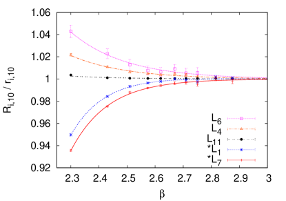
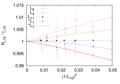
Dividing the constants $r_{ij}$ out, Figs. 10 and 11 give a visual impression of the scaling of selected fitting curves with reference scale $L_{10}$. Superficially, curves for the same scales look similar in Fig. 11 as before in Figs. 7 and 8. However, there is a fundamental difference between the fits. Equation (45) ensures that $L_{i}/L_{10}\sim(1/L_{10})^{2}$ is correct for in the limit $(1/L_{10})^{2}\to 0$, while in Eq. (33) it is assumed to be already exact for the data at hand. Now, for the fits (45) the straight line behavior is in some cases only reached for very small $(1/L_{10})^{2}$. This is most pronounced for the $R_{1,10}/r_{1,10}$ fit, which crosses the value 1 from below and finally approaches 1 from above, once the region $(1/L_{10})^{2}<0.005$ on the very left side of Fig. 11 is reached (details are not visible on the scale of the figure). In view of this it is reassuring that the estimates of Tables 7 and 9 never differ by more than 1.3%. The two fitting approaches supplement one another and give some insight into systematic errors one may expect.

Figure 12: Three fits of the deconfinement length scale $L_{0}$ versus $(1/L_{10})^{2}$.

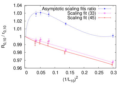
We conclude this section discussing the instabilities encountered when fitting $L_{0}/L_{i}$. In the $L_{0}$ (as) row of Table 9 we report estimates obtained from using the constants of column six of Table 8 and error propagation. Compared with the previous estimates of Table 7 we find a systematic decrease in the range 3.2% to 3.6%, larger than the statistical error, which never exceeds 0.6%. As the asymptotic scaling of $L_{0}$ needs four parameters to fit just five data points one may suspect “overfitting”. As a tiebreaker we perform the fit of Eq. (45) for jackknifed ratios of $L_{0}/L_{j}$, $j=1,4,7,10$ and obtain the estimates of the $L_{0}$ row of Table 9. The systematic errors with respect to Table 7 are now down to less than 1%.

Dividing the asymptotic ratios out, the three fits for $L_{0}/L_{10}$ are shown in Fig. 12. The straight line fit from Figs. 6 and 7 comes in as second lowest. The lowest curve corresponds to Eq. (45) and the upper curve to dividing the $L_{0}$ fit of column six of Table 8 by the $L_{10}$ fit of the same column. As suspected this curve looks rather fanciful. However, using a log scale for the abscissa would stretch the range on the left, and one should have in mind that the absolute differences between all three fits are quite small. Systematic errors at $(1/L_{10})^{2}=0.3$ can be read off on the right-hand side of the figure and are seen to be less than 4%.

VI Summary and conclusions

We have studied the approach of SU(2) LGT to its quantum continuum limit by investigating the scaling behavior of a number of length scales with definitions based on the deconfinement phase transition, the gradient flow and the cooling flow. While the deconfining scale $L_{0}=N_{\tau}$ is uniquely defined (4), one has considerable freedom in the definition of gradient and cooling flow scales. They depend on the choice of observables and target values of the flow. We considered:

1. Energy densities $E_{0}$, $E_{1}$, $E_{4}$ defined by Eqs. (16, 17, 18). $E_{0}$ is up to normalization the Wilson action and $E_{1}$ in essence an equivalent definition. $E_{4}$, introduced in L10 , averages over four plaquettes.

2. Target values $y^{01}_{i}$ and $y^{02}_{i}$, ($i=0,1,4$) are defined by Eqs. (23, 24, 29, 30). They are constructed so that the initial scaling behavior of either the gradient or the cooling flow of either $E_{0}$, $E_{1}$ or $E_{4}$ matches that of the deconfinement length $N_{\tau}$ (altogether $3\times 4=12$ distinct definitions).

For ratios of these length scales, corrections to scaling are supposed to be of order $a^{2}$ in the lattice spacing as illustrated in Figs. 6, 7, 8, 11 and 12. In these figures the cooling length scale $L_{10}$, which relies on the $E_{0}$ energy density and a $y^{02}_{0}$ target value (30), is used as reference scale by the following reasons:

1. Scaling violations of ratios of scales are then rather symmetrically distributed above and below 1.

2. $E_{0}$ is easier to calculate than $E_{4}$ and estimates from the same statistics result in smaller error bars for the $E_{0}$ length scale. No scaling advantages were found for $E_{4}$ scales. $E_{1}$ is essentially equivalent to $E_{0}$ with the benefit for $E_{0}$ that the Wilson action is implemented in the program anyhow.

3. The cooling flow is faster and easier to calculate than the gradient flow and there is no noticeable loss of accuracy as anticipated in Ref. BD14 . As the cooling method B81 was an answer to difficulties encountered when trying to calculate the topological charge in a paper by Lüscher and one of the authors BL81 , it appears that the cooling scale could have been introduced 30 years before the gradient scale L10 .

The magnitude of scaling violations we find for ratios of length scales is close to that reported in Ref. L10 for SU(3) when comparing the $E_{0}$ with the $E_{4}$ flow. The SU(2) scaling region begins at $\beta=2.3$ where we find corrections to scaling in the 10% range. Deeper in the scaling region, at $\beta=2.46$, they become reduced to slightly less than 5%.

Scaling corrections for the ratio $N_{\tau}/L_{10}$ fall into the range provided by the other scales as is seen in Figs. 6 and 7. The significant advantage of the gradient scale, and to an even greater extent the cooling scale, over the deconfinement scale is that we can far more easily follow the scaling behavior towards the continuum limit. On the other hand, there are no ambiguities in the definition of the deconfinement scale, which makes it kind of ideal to define initial scaling values as discussed in sections III and IV.

We have used two rather different approaches for analyzing our data. For Figs. 6 to 8 we simply calculate $L_{i}/L_{10}$ from jackknife bins of the data and perform the linear 2-parameter fit (33) using the ${\cal O}(a^{2})$ dependence $(1/L_{10})^{2}$ from the same data. While this is straightforward, one does not connect with the asymptotic $\Lambda_{L}$ scale.

To connect with asymptotic scaling, we relied on truncated forms of Eq. (34) based on Ref. A97 ; B15 . The normalization constants of our asymptotic scaling fits are collected in Table 8. A common fixed parameter ensures that scaling corrections for ratios are ${\cal O}(a^{2})$. Systematic errors due to distinct truncations of the fits are found around 10%. For the gradient and cooling scales the finally accepted fits of column six rely on three free parameters, one of them being the normalization constant that yields the continuum estimate. For $L_{0}$ four fit parameters are needed despite the fact that there are only five data points. Comparing in Fig. 12 the ratio of the $L_{0}$ and $L_{10}$ fit with direct fits of the $R_{0,10}$ ratios indicates overfitting, though $L_{0}$ data on larger lattices is needed to be conclusive.

While the lattice spacing is exponentially small in $\beta$, asymptotic scaling corrections come in powers of $1/\beta$. As is seen in Fig. 9, they range at $\beta=2.3$ from 30% to 36%. The scales cluster together, so that the relative deviations at $\beta=2.3$ reproduce the previously encountered 10% range.

For ratio estimates it turns out that one should not divide the asymptotic scaling estimates by one another, but perform the fit (45) for the jackknifed $R_{ij}$ ratios of the data, where the common fixed parameter is set to zero to enforce ${\cal O}(a^{2})$ corrections. A decisive difference to the previous approach (33) remains: The ${\cal O}(a^{2})$ behavior is no longer enforced for our data at hand, but only in the continuum limit. Indeed, some of the fits make use of this possibility. Compare Fig. 11 with Figs. 7 and 8. Despite the differences in the approach to the continuum limit, the obtained curves look similar.

The continuum limit estimates of our ratios are collected in Tables 7 and 9 using, respectively, (33) and (45). Differences due to the distinct fit forms stay below 1.3%. This is in most cases larger than the statistical errors. The different fit forms allow one to get an idea of the systematic errors possible.

In conclusion, we hope that the methods outlined are also of some value for studying the approach of physically realistic theories like QCD to their continuum limits. Though such data rely on large scale calculations on supercomputers, it is presumably safe to assume that their quality is not better than that of our SU(2) data.