Superconducting grid-bus surface code architecture for hole-spin qubits

Abstract

We present a scalable hybrid architecture for the 2D surface code combining superconducting resonators and hole-spin qubits in nanowires with tunable direct Rashba spin-orbit coupling. The back-bone of this architecture is a square lattice of capacitively coupled coplanar waveguide resonators each of which hosts a nanowire hole-spin qubit. Both the frequency of the qubits and their coupling to the microwave field are tunable by a static electric field applied via the resonator center pin. In the dispersive regime, an entangling two-qubit gate can be realized via a third order process, whereby a virtual photon in one resonator is created by a first qubit, coherently transferred to a neighboring resonator, and absorbed by a second qubit in that resonator. Numerical simulations with state-of-the-art coherence times yield gate fidelities approaching the $99\%$ fault tolerance threshold.

Scalability is central to the ongoing efforts towards fault tolerant quantum computation Taylor et al. (2005); Chen et al. (2014); Nemoto et al. (2014); Hill et al. (2015); Billangeon et al. (2015); Brecht et al. (2016); Karzig et al. (2016). Owing to its high error rate threshold and its benign requirement of only local qubit interactions, the surface code Bravyi and Kitaev (1998) is a promising candidate to achieve fault tolerance. Superconducting circuits, with their long coherence times and high-level of controlability, have emerged as an ideal platform for a physical implementation of the surface code Helmer et al. (2009); DiVincenzo (2009); Fowler et al. (2012); Barends et al. (2014); Corcoles et al. (2015); Kelly et al. (2015); Takita et al. (2016). At the heart of this approach lies the coherent light-matter interaction between the electric dipole moment of a superconducting condensate and quantized microwave fields Blais et al. (2004). This interaction however is a double-edged sword. On the upside, it enables the readout and control of superconducting qubits and of their interaction with each other via the quantum bus Blais et al. (2007); Majer et al. (2007). On the downside, the presence of an electric dipole moment means that un-monitored degrees of freedom, such as thermal and quantum fluctuations of the field, couple to the qubits and limit their coherence Gambetta et al. (2006). Moreover, in a multi-qubit system, the accumulation of errors due to off-resonant couplings represents a serious problem for scalability Corcoles et al. (2015); Kelly et al. (2015); Blumoff et al. (2016); Takita et al. (2016). The ability to tune the light-matter coupling on and off on-demand is thus highly desirable. Superconducting qubits with tunable qubit-resonator coupling have been realized Gambetta et al. (2011); Srinivasan et al. (2011); Eichler et al. (2015); Zhang et al. (2016), but their robustness is limited since they rely on quantum coherent interference at a symmetry point.

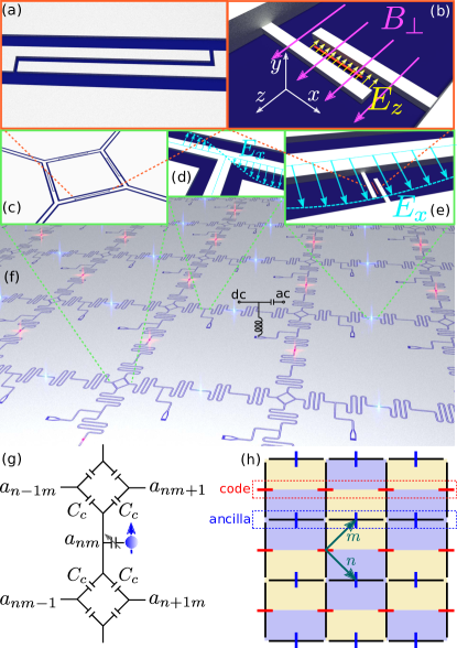
Figure 1: Grid-bus surface code architecture. (a) and (c): Four-way capacitor design minimizing undesired cross-couplings. (b) and (e): A nanowire hole-spin qubit inside a capacitor in the trench of the resonator. The electric field perpendicular to the wire $E_{z}$ is controlled by voltage biasing the center conductor via the bias-tee shown in (f). (d): Resonator drive port placed at a node of the ac field $E_{x}$. (f): Resonator grid layout. The light gray areas represent the superconductor thin film on top of the dielectric substrate (dark blue). The red and blue dots at the center of each resonator indicate the positions of the nanowire qubits. (g): Each resonator couples to four neighboring resonators. (h): Resonator (black lines) and qubits (red and blue bars) arranged in a square lattice. The red bars denote code qubits while the blue bars denote ancilla qubits. The colored rectangles represent the two types of plaquettes of the surface code (e.g. $XXXX$ or $ZZZZ$). The basis vectors on the lattice are indicated by dark green arrows labeled $n$ and $m$.

The recent discovery by Kloeffel et al. (2011) of an electrically induced spin-orbit interaction of Rashba type in the low energy hole states of Ge/Si (core/shell) nanowires provides an attractive alternative to realize a tunable coupling qubit. In this case the qubit is encoded in two orthogonal dressed spin states of a hole confined in a nanowire quantum dot. Hole spins are particularly attractive since their p-wave orbitals have minimal overlap with the nuclei resulting in long coherence times Hu et al. (2012); Kloeffel et al. (2013); Prechtel et al. (2016); Watzinger et al. (2016) and have recently been demonstrated to be compatible with industrial CMOS technology Maurand et al. (2016). Crucially the strong direct Rashba spin-orbit interaction (DRSOI) is controlled by an external electric field applied perpendicular to the wire Kloeffel et al. (2011, 2013). This enables the electrostatic control of the coupling between the spin degree of freedom and the electromagnetic field along the wire.

In this letter, we propose a scalable surface code architecture obtained by combining nanowire hole-spin qubits with a novel coplanar waveguide resonator grid structure. The latter can be viewed as a generalization of the celebrated 1D quantum bus architecture Blais et al. (2007); Majer et al. (2007) to two dimensions. Furthermore, owing to the small size of the nanowire qubits, a few tens of nanometers in length, they can be entirely embedded within the microwave resonators allowing for more compact resonator geometries with enhanced vacuum field strengths. The electrostatic fields required to tune the microwave-qubit coupling, are provided in-situ by voltage biasing the resonator center conductor thus reducing the number of required leads.

The system we consider is depicted schematically in Fig. 1. It consists of a square lattice of coplanar microwave resonators, with a nanowire qubit placed at the field anti-node of each resonator. Here we consider full-wave resonators where the resonator length equals the wavelength $\lambda$ and the qubits are placed at the central anti-node. Each resonator is capacitively coupled to four neighboring resonators forming a horizontal “H” shape as shown in Fig. 1 (g). The nanowires, each containing a single spin-orbit qubit, are situated inside the trenches between the center conductor and the ground plane defining the resonator, as depcited in insets (b) and (e) of Fig. 1. The qubit is thus fully embedded within the resonator. The electromagnetic fields are only weakly screened inside the semiconductor of the nanowire enabling a strong coupling between the qubit and the ac field component along the wire Kloeffel et al. (2013).

To characterize this system, we start by considering an isolated site of the lattice composed of one resonator and one hole-spin nanowire qubit. The nanowire is oriented along the $x$-axis and a magnetic field is applied along $z$. We describe the hole harmonically confined along the wire by the 1D effective Hamiltonian Maier et al. (2014)

$$\bm{H}_{h}=\frac{\bm{p}^{2}}{2m}+\frac{1}{2}m\omega_{h}^{2}\bm{x}^{2}+\alpha_{\rm DR}\bm{\sigma}^{y}\bm{p}+\frac{g\mu_{\rm B}B_{\perp}}{2}\bm{\sigma}^{z}.$$ (1)

Here $\alpha_{\rm DR}$ is the strength of the DRSOI and $B_{\perp}$ denotes the magnetic field strength perpendicular to the axis of the wire. The hole furthermore couples to the electromagnetic field of the resonator and this is described in dipole approximation via the Hamiltonian

$$\bm{H}_{c}=eE_{\rm rms}\bm{x}(\bm{a}+\bm{a}^{\dagger})+\hbar\omega_{r}\bm{a}^{\dagger}\bm{a}.$$ (2)

Here $E_{\rm rms}=\frac{1}{W}\sqrt{\frac{\hbar\omega_{r}}{cl}}$ is the $x$-component of the anti-node vacuum root mean square field of the CPW resonator with resonance frequency $\omega_{r}$, trench width $W$, length $l$ and capacitance per unit length $c$. The full Hamiltonian is $\bm{H}=\bm{H}_{h}+\bm{H}_{r}$. The effect of the spin-orbit coupling is seen most clearly upon performing the unitary transformation $\bm{U}=\exp\left[i(\bm{x}/\ell_{\rm SO})\bm{\sigma}^{y}\right]$, where the spin-orbit length $\ell_{\rm SO}=\hbar/(m\alpha_{\rm DR})$ characterizes the length over which the spin flips due to spin-orbit coupling in the absence of a magnetic field. This generalizes the semiclassical approach of Flindt et al. (2006); Trif et al. (2007) to the quantum regime. In the limit where $\ell_{\rm SO}\gg x_{\rm ZPF}=\sqrt{\hbar/(2m\omega_{h})}$, the mixing of orbital and spin degrees of freedom is weak and the transformed Hamiltonian reads sup

$$\bm{H}\simeq\bm{H}_{c}+\frac{\bm{p}^{2}}{2m}+\frac{1}{2}m\omega_{h}^{2}\bm{x}^{2}+\frac{\hbar\omega_{Z}}{2}\left(\bm{\sigma}^{z}-\frac{2\bm{x}}{\ell_{\rm SO}}\bm{\sigma}^{x}\right).$$ (3)

Here we have suppressed a c-number term and defined the Zeeman frequency $\omega_{Z}=g\mu_{\rm B}B_{\perp}/\hbar$.

We are interested in the regime where $\omega_{h}\gg\omega_{r},\omega_{Z}$ such that the hole remains in its ground state. In this regime, we can adiabatically eliminate the center of mass motion of the hole sup . The dynamics of the hole-spin coupled to the resonator is then captured by an effective Jaynes-Cummings model

$$\frac{\bm{H}_{\rm JC}}{\hbar}=\omega_{r}\bm{a}^{\dagger}\bm{a}+\frac{\omega_{Z}^{\prime}}{2}\bm{\sigma}^{z}+\nu\left(\bm{a}\bm{\sigma}^{+}+\bm{a}^{\dagger}\bm{\sigma}^{-}\right),$$ (4)

where the transition frequency of the qubit is determined by the renormalized Zeeman splitting

$$\omega_{Z}^{\prime}=\omega_{Z}\left[1-\frac{\omega_{Z}}{\omega_{h}-\omega_{Z}}\left(\frac{x_{\rm ZPF}}{\ell_{\rm SO}}\right)^{2}\right],$$ (5)

and the spin-field coupling strength is given by

$$\nu=\frac{\beta\omega_{Z}}{\omega_{h}-\omega_{r}}\left(\frac{x_{\rm ZPF}}{\ell_{\rm SO}}\right).$$ (6)

Here $\beta=eE_{\rm rms}x_{\rm ZPF}$ is the dipole coupling strength between the hole in the motional ground state and the vacuum field of the resonator. Importantly $\ell_{\rm SO}$ depends, via the spin-orbit coupling strength $\alpha_{\rm DR}$, on the electric field component $E_{z}$ perpendicular to the wire. In the weak field limit $\alpha_{\rm DR}\propto E_{z}$ and so the coupling $\nu$ increases linearly with $E_{z}$ while $\omega_{Z}^{\prime}$ decreases quadratically. Thus the “off” state, $E_{z}=0$, corresponds to a sweet-spot for the qubit where it is protected against fluctuations of the electric field to linear order. A non-perturbative treatment, of which the above expressions (5) and (6) are the leading order expressions, can be found in Kloeffel et al. (2013). For Ge/Si nanowires, the Zeeman splitting in (5) reaches the GHz frequency regime for magnetic field strengths around one hundred milli Tesla. We emphasize that our architecture is compatible with a magnetic field parallel to the plane of the superconducting resonator, mitigating adverse effects on the resonator quality factor Samkharadze et al. (2016). A strength of our architecture is that the required electrostatic control field can be generated without the need for additional bias lines. This is achieved by applying a voltage bias between the center conductor and the ground plate of the resonator via a low-pass filtered T-junction contact formed at a field node as depicted in inset (d) of Fig. 1. By using a bias-tee, the same port can be used to drive the resonator. When the qubit-resonator coupling is on, this enables fast qubit rotations around any axis in the $x-y$ plane of the Bloch sphere.

Scaling up, we next consider an $N\times M$ lattice of such resonators, where each resonator is coupled capacitively to four neighboring resonators as illustrated in Fig. 1 (g). A global in-plane magnetic field is applied at an angle with the nanowires (ideally $\pi/4$ for equal strength coupling to nanowires in both orientations). Because of the strong suppression of the g-factor along the axis of the wires Maier et al. (2013); Brauns et al. (2016), we consider for each wire only the perpendicular component of the magnetic field justifying the applicability of Eq. (4) also in this case. In the rotating wave approximation, the dynamics on the lattice can be modeled by the Jaynes-Cummings-Hubbard Hamiltonian Zhu et al. (2013)

$$\frac{\bm{H}}{\hbar}=\sum_{n=1}^{N}\sum_{m=1}^{M}\left[\frac{\omega_{Z}}{2}\bm{\sigma}_{nm}^{z}+\omega_{r}\bm{a}_{nm}^{\dagger}\bm{a}_{nm}+\frac{\nu_{nm}}{2}\left(\bm{a}_{nm}\bm{\sigma}_{nm}^{+}+{\rm h.c.}\right)\right]$$ (7)

$$+J\sum_{n,m}\left(\bm{a}_{nm}^{\dagger}\bm{a}_{nm+1}+\bm{a}_{nm}^{\dagger}\bm{a}_{nm-1}+\bm{a}_{nm}^{\dagger}\bm{a}_{n+1m}+\bm{a}_{nm}^{\dagger}\bm{a}_{n-1m}+{\rm h.c.}\right).$$

The inter-resonator coupling strength is given by $J=2\hbar\omega_{r}\frac{C_{c}}{C+4C_{c}}$, in terms of the mode frequency $\omega_{r}$, the coupling capacitance $C_{c}$ and the effective self-capacitance of the resonator mode $C=cl$. The tunable spin-resonator coupling of lattice site $(n,m)$ is denoted with $\nu_{nm}$.

A scalable implementation of the surface code requires:

• Two-qubit gates between nearest neighbors on a lattice.

• Arbitrary single-qubit rotations.

• Individual qubit readout in the computational basis.

• Parallelizability.

Conditions (i) and (ii) together allow one to encode the error syndrome onto ancilla qubits and (iii) allows one to read out the error syndrome. Condition (iv) means that the gates must be performed in parallel so that the time for a single syndrome measurement cycle does not increase with the lattice size. In theory all stabilizer operator measurements could be done simultaneously, since per definition the stabilizer operators commute with each other. However, in practice when the measurements of multi-qubit stabilizer operators are decomposed into sequences of single and two-qubit gates between pairs of qubits, a certain degree of sequentiality is unavoidable. In the following we show how our architecture meets the requirements (i) to (iv).

Single-qubit gates. To address a particular qubit, the center conductor of the corresponding resonator is voltage biased, generating an electric field $E_{z}=E_{z}^{*}$ perpendicular to the wire (see Fig. 1 (b)). This effectively turns on the DRSOI and couples the qubit to the ac field. Single-qubit rotations around any axis in the $x-y$ plane of the Bloch-sphere can then be performed in a standard way Blais et al. (2004), by driving the resonator mode at the Lamb and Stark shifted qubit resonance frequency with a coherent microwave drive of appropriate phase (see Fig. 3 (a) and sup ). By concatenating rotations around different axes, arbitrary rotations on the Bloch sphere can be generated. Interestingly, the electric tunability of the Zeeman splitting provides a shortcut for single-qubit phase gates: To acquire a phase $\theta$ one simply has to bias the center conductor for a duration $T=\theta/\Delta\omega_{Z}$ with $\Delta\omega_{Z}=\omega_{Z}(E_{z}=0)-\omega_{Z}(E_{z}=E_{z}^{*})$. Because each resonator is coupled only to its four orthogonal neighboring resonators, single-qubit gates can be performed in parallel on all code qubits and separately on all ancilla qubits by alternatingly coupling one set of qubits to the grid-bus while the other remains uncoupled.

Nearest neighbor two-qubit gates. A high fidelity two-qubit gate can be realized by a generalization of the resonator-bus mediated qubit-qubit flip-flop interaction Blais et al. (2004, 2007); Kloeffel et al. (2013). Since each qubit is directly coupled only to one resonator, a virtual photon emitted by the first qubit needs to hop from one resonator to a neighboring one before being absorbed by the second qubit (see Fig. 3 (b)). A perturbative analysis sup gives an effective coupling between qubits at sites $(n,m)$ and $(n^{\prime},m^{\prime})$ of the form

$$\bm{H}_{XY} =\sum_{nm,n^{\prime}m^{\prime}}K_{nm,n^{\prime}m^{\prime}}\bm{\sigma}_{nm}^{+}\bm{\sigma}_{n^{\prime}m^{\prime}}^{-}+{\rm h.c.}$$ (8)

where, in the weak coupling regime $J\ll|\omega_{Z}-\omega_{r}|$, the coupling strength is given by sup

$$K_{nm,n^{\prime}m^{\prime}} =\frac{(\Delta m+\Delta n)!}{\Delta n!\Delta m!}\frac{\nu_{nm}\nu_{n^{\prime}m^{\prime}}}{\Delta}\left(\frac{J}{\Delta}\right)^{\Delta m+\Delta n},$$ (9)

with $\Delta n=|n-n^{\prime}|$, $\Delta m=|m-m^{\prime}|$ and $\Delta=\omega_{r}-\omega_{Z}$. The coupling strength decays exponentially with distance on the lattice and the nearest neighbor coupling strength (i.e. for $n^{\prime}=n$ and $m^{\prime}=m\pm 1$ or $n^{\prime}=n\pm 1$ and $m^{\prime}=m$), is sup

$$K_{\rm NN}\simeq\frac{J}{\Delta^{2}}\nu_{nm}\nu_{n^{\prime}m^{\prime}}.$$ (10)

Compared with the usual flip-flop interaction strength between two qubits off-resonantly coupled to the same resonator mode, this coupling is a factor $J/|\Delta|$ smaller as it involves an additional off-resonant inter-resonator photon hopping. The interaction (8) acting for a duration $T$, naturally gives rise to the $\sqrt{i\rm SWAP}$ gate when $K_{\rm NN}T=\pi/4$. Two such gates together with single-qubit rotations can be used to implement the CNOT gates required for syndrome measurements in the surface code. As with the single-qubit gates, it is possible to perform many two-qubit gates in parallel by taking advantage of the electric field tunability of the qubit frequency. This is achieved by separating the qubits on the lattice into two sets with frequencies $\omega_{Z}^{\rm(r)}$ and $\omega_{Z}^{\rm(b)}$ as illustrated in Fig. 2. A full syndrome mapping cycle from the code qubits onto the ancilla qubits can then be performed in four steps.

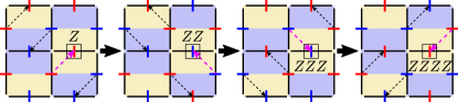
Figure 2: Frequency layout for parallelization of syndrome mapping in four steps. Red (blue) bars denote qubits at frequency $\omega_{Z}^{\rm(r)}$ ($\omega_{Z}^{\rm(b)}$). The dashed black arrows indicate which couplings are resonant, i.e. active in a given configuration. The mapping of a $ZZZZ$ stabilizer is highlighted as an example (magenta arrows).

Readout. The readout of the ancilla qubits proceeds in standard fashion by homodyne detection of the dispersive phase shift incurred by reflected photons at the bare resonator frequency Blais et al. (2007); Koch et al. (2007). During readout the code qubits are decoupled from their resonators. Similar to single-qubit operations, readout of all ancilla qubits can be performed in parallel and does not require additional resonators, greatly simplifying the circuit design. The required reset of the ancilla qubits to their groundstate after measurement can be implemented for example by using the method of Geerlings et al. (2013).

Parameter estimates. From electrostatic finite element simulations with optimized cross capacitor designs, we find that coupling capacitances $C_{c}$ on the order of a few tens of ${\rm fF}$ can be achieved while strongly suppressing unwanted direct couplings by more than two orders of magnitude sup . With a resonator length $l=10\,{\rm mm}$ and capacitance per unit length Goppl et al. (2008) $c=0.127\,{\rm nF/m}$, this leads to a relative inter-resonator coupling strength $J/(\hbar\omega_{r})\simeq 1\%$. For the simulations presented below we take $J/\hbar=159\times 2\pi\,{\rm MHz}$, which corresponds to a coupling capacitance $C_{c}\simeq 14\,{\rm fF}$, and set the resonator frequency to $\omega_{r}=13.35\times 2\pi\,{\rm GHz}$. The hole confinement frequency is set to $\omega_{h}=28\times 2\pi\,{\rm GHz}$, which for an effective hole mass $m\simeq 0.012m_{e}$, where $m_{e}$ is the electron mass, corresponds to a zero point fluctuation $x_{\rm ZPF}\simeq 166\,{\rm nm}$. We consider a magnetic field strength $B_{\perp}=194\,{\rm mT}$, which together with a zero-field g-factor for Germanium Kloeffel et al. (2013); Watzinger et al. (2016) $g(E_{z}=0)\simeq 5.5$, corresponds to a zero-field qubit frequency $\omega_{Z}(E_{z}=0)\simeq 14.934\times 2\pi\,{\rm GHz}$. The small length of the nanowire qubits allows for a coplanar waveguide geometry with a small trench width, which we take to be $W=0.5\,{\rm\mu m}$. This enhances the root mean square electric field to about $E_{\rm rms}\simeq 3.73\,{\rm V/m}$. Finally, we assume a Rashba spin-orbit parameter $\alpha_{\rm DR}/\hbar\simeq 10\,e({\rm nm})^{2}\times E_{z}$. For an applied field $E_{z}=1\,{\rm V/\mu m}$, this corresponds to $\ell_{\rm SO}\simeq 635\,{\rm nm}$. According to Eq. (6), we thus estimate conservatively that coupling strengths between $\nu_{nm}=0$ at $E_{z}=0$ and $\nu_{nm}/\hbar\simeq 40\times 2\pi\,{\rm MHz}$ at $E_{z}=1\,{\rm V/\mu m}$ are currently feasible. The corresponding qubit frequency shift between the “on” and the “off” states is $\Delta\omega_{Z}\simeq 1.161\times 2\pi\,{\rm GHz}$, i.e. $\omega_{Z}(E_{z}=1\,{\rm V/\mu m})\simeq 13.773\times 2\pi\,{\rm GHz}$, which allows for phase gates on the nanosecond timescale.

Numerical simulations. We characterize the theoretical performance of single and two-qubit gates on a $2\times 2$ lattice in the presence of dissipation and gate imperfections by numerically solving the Lindblad master equation (with $\hbar=1$)

$$\bm{\dot{\rho}}=-i[\bm{H}+\bm{H}_{d},\bm{\rho}]+\kappa\sum_{nm}\mathcal{D}[\bm{a}_{nm}]\bm{\rho}+\gamma\sum_{nm}\mathcal{D}[\bm{\sigma}^{-}_{nm}]\bm{\rho}.$$ (11)

Here $\bm{H}$ is given by Eq. (7), $\kappa$ denotes the single photon loss rate of the resonators, $\gamma=1/T_{1}$ the qubit decay rate and $\mathcal{D}[\bm{O}]\bm{\rho}=(2\bm{O}\bm{\rho}\bm{O}^{\dagger}-\bm{O}^{\dagger}\bm{O}\bm{\rho}-\bm{\rho}\bm{O}^{\dagger}\bm{O})/2$. Fig. 3 (c) shows the fidelity of a rotation the qubit at lattice site $(0,0)$ around the $x$-axis by angle $\pi$ averaged over all initial states on the Bloch sphere as a function of the gate duration time $T$ for $\kappa/h=\gamma/h=10\,{\rm kHz}$. This rotation is realized by a drive on resonator $(0,0)$ of the form $\bm{H}_{d}(t)=\varepsilon(t)\left(e^{i\omega_{d}t}\bm{a}+e^{-i\omega_{d}t}\bm{a}^{\dagger}\right)$ with frequency $\omega_{d}=\omega_{Z}+(2\bar{n}+1)\raisebox{1.50696pt}{$\chi$}$ and gaussian envelop $\varepsilon(t)=\varepsilon\exp[-(t-t_{0})^{2}/(2\sigma^{2})]$ with $\varepsilon=\pi\Delta/(2\sigma\nu\sqrt{2\pi})$. Here $\sigma=T/5$, $t_{0}=T/2$, $\Delta=\omega_{Z}-\omega_{r}$ and $\omega_{Z}$ is the bare qubit frequency in the “on” state with dispersive shift $\raisebox{1.50696pt}{$\chi$}=\nu^{2}/\Delta$. The drive frequency shift $(2\bar{n}+1)\raisebox{1.50696pt}{$\chi$}$ with $\bar{n}\simeq\varepsilon^{2}/[\Delta^{2}+(\kappa/2)^{2}]$ corrects (approximately) for both the Lamb and Stark shifts. The simulated fidelity (full red curve in Fig. 3 (c)) is upper bounded by $\mathcal{F}_{\varphi}=(1+(1/3)e^{-\gamma T}+(2/3)e^{-\left[\gamma/2+\gamma_{\varphi}\right]T})/2$ (dashed curve in Fig. 3 (c)), which gives the average fidelity for an ideal gate with a $T_{1}$-limited qubit subject to photon shot noise induced dephasing Gambetta et al. (2006) with rate $\gamma_{\varphi}\simeq 2\bar{n}\kappa(\pi/2)^{2}$ (blue curve in Fig. 3 (c)). The difference between the two curves is a measure of gate imperfections such as deviations from optimal pulse duration and spurious entanglement between the photons and the qubit, which increases with the drive strength.

Next we characterize the natural two-qubit gate generated by the interaction in Eq. (8). Fig. 3 (d) shows the fidelity of a $\sqrt{i{\rm SWAP}}=\sqrt{1/2}\,[\openone+\bm{ZZ}-i(\bm{XX}+\bm{YY})]^{1/2}$ gate between qubits at sites $(0,0)$ and $(0,1)$ obtained for $K_{\rm NN}T=\pi/4$, averaged over the subset of initial two-qubit states in ${\rm span}\,\{\ket{eg},\ket{ge}\}$, while the remaining two qubits are in their ground state. In this case, the gate duration $T$ is fixed by the interaction strength. The latter however depends on the strength of the applied electric field $E_{z}$. For small $E_{z}$ the averaged gate fidelity agrees well with that of an ideal $T_{1}$-limited $\sqrt{i{\rm SWAP}}$ gate, which for the considered initial states in the one-excitation manifold, is simply $\mathcal{F}_{0}=e^{-\gamma T}$ (dashed curve in Fig. 3 (d)). As the field and hence the interaction strength is increased, the gate becomes faster and, at first, the fidelity increases. Because an increasing electric field also reduces the detuning between the qubit and the resonator, the dispersive approximation breaks down for too large an applied field, which is reflected in fluctuations and overall suppression of the fidelity at strong fields.

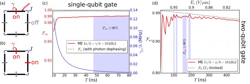
Figure 3: Gate fidelity averaged over initial states on the Bloch sphere: $\mathcal{F}_{\rm av}=\frac{1}{4\pi}\int_{0}^{2\pi}{\rm d}\varphi\int_{0}^{\pi}{\rm d}\theta\sin(\theta)\mathcal{F}(\theta,\varphi)$, with $\mathcal{F}(\theta,\varphi)=\mathinner{\langle{\theta,\varphi|\bm{\rho}(T)|\theta,\varphi}\rangle}$ and $\ket{\theta,\varphi}=\cos\left(\frac{\theta}{2}\right)\ket{0}+e^{i\varphi}\sin\left(\frac{\theta}{2}\right)\ket{1}$. (a) and (c): Single-qubit rotation around the $x$-axis by angle $\pi$. Here $\ket{0}=\ket{g}_{00}$, $\ket{1}=\ket{e}_{00}$, the remaining qubits are initialized in their ground state. Only the qubit at $(0,0)$ is coupled to its resonator with $E_{z}=0.8\,{\rm V/\mu m}$ and the drive strength is varied. The ideal gate unitary is $R_{x}(\pi)=e^{-i\frac{\pi}{2}{\bm{\sigma}}^{x}_{00}}$. (b) and (d): Two-qubit $\sqrt{i\rm SWAP}$ gate. Here $\ket{0}=\ket{g}_{00}\ket{e}_{01}$, $\ket{1}=\ket{e}_{00}\ket{g}_{01}$, the other qubits are initialized in their ground state. The qubits at $(0,0)$ and $(0,1)$ are coupled to their resonators with varying but equal field strength $E_{z}$. The ideal gate unitary is $\sqrt{i\rm SWAP}=e^{-i\frac{\pi}{4}(\bm{\sigma}_{00}^{+}\bm{\sigma}_{01}^{-}+\bm{\sigma}_{00}^{-}\bm{\sigma}_{01}^{+})}$. Full curves are numerical results obtained by solving the master equation (ME) (11) and dashed curves show analytic upper bounds for ideal gates sup .

Conclusion. We have proposed a scalable hybrid architecture for fault tolerant quantum computation via the surface code. The core of this system consists of a square lattice of capacitively coupled superconducting resonators, which serves as a two-dimensional quantum bus to mediate interactions between nanowire hole-spin qubits. By leveraging the electric tunability of the strong DRSOI, unwanted couplings between qubits are suppressed. This is a key advantage compared to other architectures where qubit-qubit interactions are controlled by frequency tuning and errors due to spurious off-resonant couplings scale with the system size. Furthermore, the circuit layout of our architecture benefits from the small size of the nanowire qubits and is greatly simplified by efficient component reuse.

Acknowledgments. This work was supported by the Swiss National Science Foundation (SNSF) and the NCCR QSIT. D. L. acknowledges James Wootton for useful discussions. The numerical computations were peformed in a parallel computing environment at sciCORE (http://scicore.unibas.ch/) scientific computing core facility at University of Basel using the Python library QuTip (http://qutip.org/).

I Derivation of Eqs. (3) and (4)

Here we derive the effective model, Eq. (4) of the main text. We start from the Hamiltonian given by the sum of Eqs. (1) and (2) in the main text which is

$$\bm{H}=\frac{\bm{p}^{2}}{2m}+\frac{1}{2}m\omega_{h}^{2}\bm{x}^{2}+\alpha_{\rm DR}\bm{\sigma}^{y}\bm{p}+\frac{\hbar\omega_{Z}}{2}\bm{\sigma}^{z}+eE_{\rm rms}\bm{x}(\bm{a}+\bm{a}^{\dagger})+\hbar\omega_{r}\bm{a}^{\dagger}\bm{a}.$$ (S12)

We note that in the absence of a magnetic field, i.e. $\omega_{Z}=0$, the spin degree of freedom is conserved as $[\bm{\sigma}^{y},\bm{H}|_{B=0}]=0$. We first remove the spin-orbit term by performing a spin conditional momentum displacement via the unitary operator

$$\bm{U}=\exp\left(i\frac{\bm{x}}{\ell_{\rm SO}}\bm{\sigma}^{y}\right),\quad\ell_{\rm SO}\equiv\frac{\hbar}{m\alpha_{\rm DR}}.$$ (S13)

The transformed Hamiltonian is

$$\bm{\tilde{H}}=\bm{U}\bm{H}\bm{U}^{\dagger} =\frac{\left(\bm{p}-\frac{\hbar}{\ell_{\rm SO}}\bm{\sigma}^{y}\right)^{2}}{2m}+\alpha_{\rm DR}\bm{\sigma}^{y}\left(\bm{p}-\frac{\hbar}{\ell_{\rm SO}}\bm{\sigma}^{y}\right)+\frac{1}{2}m\omega_{h}^{2}\bm{x}^{2}+eE_{\rm rms}\bm{x}\left(\bm{a}+\bm{a}^{\dagger}\right)+\hbar\omega_{r}\bm{a}^{\dagger}\bm{a}$$ (S14a)

$$+\frac{\hbar\omega_{Z}}{2}\left[\cos\left(\frac{\bm{x}}{\ell_{\rm SO}}\right)+i\sin\left(\frac{\bm{x}}{\ell_{\rm SO}}\right)\bm{\sigma}^{y}\right]\bm{\sigma}^{z}\left[\cos\left(\frac{\bm{x}}{\ell_{\rm SO}}\right)-i\sin\left(\frac{\bm{x}}{\ell_{\rm SO}}\right)\bm{\sigma}^{y}\right]$$ (S14b)

$$=\frac{\bm{p}^{2}}{2m}+\frac{1}{2}m\omega_{h}^{2}\bm{x}^{2}+eE_{\rm rms}\bm{x}\left(\bm{a}+\bm{a}^{\dagger}\right)+\hbar\omega_{r}\bm{a}^{\dagger}\bm{a}+\frac{\hbar\omega_{Z}}{2}\left[\cos\left(\frac{2\bm{x}}{\ell_{\rm SO}}\right)\bm{\sigma}^{z}-\sin\left(\frac{2\bm{x}}{\ell_{\rm SO}}\right)\bm{\sigma}^{x}\right].$$ (S14c)

In the last equality, we have neglected a c-number term: $-\hbar^{2}/(2m\ell_{\rm SO}^{2})$. Note that although we have formally removed the spin-orbit term, the spin and orbital degrees of freedom of the hole are now mixed. We are primarily interested in a situation where the hole occupies the ground state of the harmonic confinement potential and where the ac field frequency is much lower than the confinement frequency i.e. $\omega_{r}\ll\omega_{h}$, such that the hole follows the field adiabatically. If further $x_{\rm ZPF}=\sqrt{\hbar/(2m\omega_{h})}\ll\pi\ell_{\rm SO}$, then the size of the hole dipole is small compared with the SOI length and we can expand the trigonometric functions to leading order yielding

$$\bm{\tilde{H}}\simeq\frac{\bm{p}^{2}}{2m}+\frac{1}{2}m\omega_{h}^{2}\bm{x}^{2}+eE_{\rm rms}\bm{x}\left(\bm{a}+\bm{a}^{\dagger}\right)+\hbar\omega_{r}\bm{a}^{\dagger}\bm{a}+\frac{\hbar\omega_{Z}}{2}\left(\bm{\sigma}^{z}-\frac{2\bm{x}}{\ell_{\rm SO}}\bm{\sigma}^{x}\right).$$ (S15)

This is Eq. (3) of the main text. Writing the position and momentum operators of the hole in second quantized notation as $\bm{x}=x_{\rm ZPF}\left(\bm{b}+\bm{b}^{\dagger}\right)$ and $\bm{p}=-\frac{i\hbar}{2x_{\rm ZPF}}\left(\bm{b}-\bm{b}^{\dagger}\right)$, the Hamiltonian becomes (we henceforth drop the $\sim$ and suppress constant c-number terms)

$$\bm{H} =\hbar\omega_{h}\bm{b}^{\dagger}\bm{b}+\hbar\omega_{r}\bm{a}^{\dagger}\bm{a}+\beta\left(\bm{a}+\bm{a}^{\dagger}\right)\left(\bm{b}+\bm{b}^{\dagger}\right)+\frac{\hbar\omega_{Z}}{2}\bm{\sigma}^{z}-\hbar\omega_{Z}\left(\frac{x_{\rm ZPF}}{\ell_{\rm SO}}\right)\left(\bm{b}+\bm{b}^{\dagger}\right)\bm{\sigma}^{x},$$ (S16)

where we have defined $\beta=eE_{\rm rms}x_{\rm ZPF}$. Further assuming that $|\omega_{Z}-\omega_{h}|\ll|\omega_{Z}+\omega_{h}|$, as well as $|\omega_{h}-\omega_{r}|\ll|\omega_{r}+\omega_{h}|$, we perform two rotating wave approximations to neglect counter-rotating terms $\sim\bm{b}^{2},\bm{b}^{\dagger 2},\bm{a}\bm{b},\bm{a}^{\dagger}\bm{b}^{\dagger}$. Thus

$$\bm{H} =\hbar\omega_{h}\bm{b}^{\dagger}\bm{b}+\hbar\omega_{r}\bm{a}^{\dagger}\bm{a}+\beta\left(\bm{a}\bm{b}^{\dagger}+\bm{a}^{\dagger}\bm{b}\right)+\frac{\hbar\omega_{Z}}{2}\bm{\sigma}^{z}-\hbar\omega_{Z}\left(\frac{x_{\rm ZPF}}{\ell_{\rm SO}}\right)\left(\bm{b}\bm{\sigma}^{+}+\bm{b}^{\dagger}\bm{\sigma}^{-}\right),$$ (S17)

We next perform the canonical transformation

$$\bm{a} =\cos(\theta)\bm{c}+\sin(\theta)\bm{d},$$ (S18)

$$\bm{b} =-\sin(\theta)\bm{c}+\cos(\theta)\bm{d}.$$ (S19)

The condition that off-diagonal elements in $\bm{c}$ and $\bm{d}$ should vanish yields the equality

$$\beta\left(\cos^{2}\theta-\sin^{2}\theta\right)=\sin\theta\cos\theta\left(\hbar\omega_{h}-\hbar\omega_{r}\right)\Leftrightarrow\theta=\frac{1}{2}\arctan\left[\frac{2\beta}{\hbar\omega_{h}-\hbar\omega_{r}}\right].$$ (S20)

In this basis, the Hamiltonian reads

$$\frac{\bm{H}}{\hbar}=\omega_{d}\bm{d}^{\dagger}\bm{d}+\omega_{c}\bm{c}^{\dagger}\bm{c}+\frac{\omega_{Z}}{2}\bm{\sigma}^{z}+\omega_{Z}\sin\left(\theta\right)\left(\frac{x_{\rm ZPF}}{\ell_{\rm SO}}\right)\left(\bm{c}^{\dagger}\bm{\sigma}^{-}+\bm{c}\bm{\sigma}^{+}\right)-\omega_{Z}\cos(\theta)\left(\frac{x_{\rm ZPF}}{\ell_{\rm SO}}\right)\left(\bm{d}^{\dagger}\bm{\sigma}^{-}+\bm{d}\bm{\sigma}^{+}\right).$$ (S21)

Here

$$\hbar\omega_{d} =\hbar\omega_{r}\sin^{2}\theta+\hbar\omega_{h}\cos^{2}\theta+2\beta\sin\theta\cos\theta,$$ (S22)

$$\hbar\omega_{c} =\hbar\omega_{r}\cos^{2}\theta+\hbar\omega_{h}\sin^{2}\theta-2\beta\sin\theta\cos\theta.$$ (S23)

We assume that $\beta\ll\hbar|\omega_{h}-\omega_{r}|$ and consequently approximate $\theta\simeq\beta/(\hbar\omega_{h}-\hbar\omega_{r})$ so that $\cos(\theta)\simeq 1$ and $\sin(\theta)\simeq\beta/(\hbar\omega_{h}-\hbar\omega_{r})$ and $\hbar\omega_{d}\simeq\hbar\omega_{h}+2\beta^{2}/(\hbar\omega_{h}-\hbar\omega_{r})\simeq\hbar\omega_{h}$ as well as $\hbar\omega_{c}\simeq\hbar\omega_{r}-2\beta^{2}/(\hbar\omega_{h}-\hbar\omega_{r})\simeq\hbar\omega_{r}$. The Hamiltonian is then

$$\frac{\bm{H}}{\hbar}\simeq\omega_{h}\bm{d}^{\dagger}\bm{d}+\omega_{r}\bm{c}^{\dagger}\bm{c}+\frac{\omega_{Z}}{2}\bm{\sigma}^{z}+\frac{\beta\omega_{Z}}{\hbar(\omega_{h}-\omega_{r})}\left(\frac{x_{\rm ZPF}}{\ell_{\rm SO}}\right)\left(\bm{c}^{\dagger}\bm{\sigma}^{-}+\bm{c}\bm{\sigma}^{+}\right)-\omega_{Z}\left(\frac{x_{\rm ZPF}}{\ell_{\rm SO}}\right)\left(\bm{d}^{\dagger}\bm{\sigma}^{-}+\bm{d}\bm{\sigma}^{+}\right).$$ (S24)

Next, we focus on the regime where

$$\frac{\omega_{h}}{\omega_{Z}}-1\gg\frac{x_{\rm ZPF}}{\ell_{\rm SO}}.$$ (S25)

and perform a Schieffer-Wolff transformation with

$$\bm{U}_{\rm SW}=\exp\left[\frac{\omega_{Z}}{\omega_{h}-\omega_{Z}}\left(\frac{x_{\rm ZPF}}{\ell_{\rm SO}}\right)\left(\bm{d}^{\dagger}\bm{\sigma}^{-}-\bm{d}\bm{\sigma}^{+}\right)\right].$$ (S26)

To leading order we find

$$\bm{H}\simeq\hbar\omega_{h}\bm{d}^{\dagger}\bm{d}+\raisebox{1.50696pt}{$\chi$}\bm{d}^{\dagger}\bm{d}\bm{\sigma}^{z}+\hbar\omega_{r}\bm{c}^{\dagger}\bm{c}+\frac{\hbar\omega_{Z}^{\prime}}{2}\bm{\sigma}^{z}+\frac{\beta\omega_{Z}}{\omega_{h}-\omega_{r}}\left(\frac{x_{\rm ZPF}}{\ell_{\rm SO}}\right)\left(\bm{c}^{\dagger}\bm{\sigma}^{-}+\bm{c}\bm{\sigma}^{+}\right),$$ (S27)

where

$$\hbar\omega_{Z}^{\prime} \simeq\hbar\omega_{Z}-\raisebox{1.50696pt}{$\chi$},\,\quad\raisebox{1.50696pt}{$\chi$}\simeq\frac{\hbar\omega_{Z}^{2}}{\omega_{h}-\omega_{Z}}\left(\frac{x_{\rm ZPF}}{\ell_{\rm SO}}\right)^{2}.$$ (S28)

As stated previously, we are interested in the situation where the hole remains in the ground state of the confinement potential. At zero temperature we can then neglect the dynamics of the $\bm{d}$ mode and obtain the final effective model for the hole-spin qubit coupled to the resonator mode (note that $\bm{c}\simeq\bm{a}$ in the considered regime)

$$\bm{H}_{\rm eff}=\hbar\omega_{r}\bm{a}^{\dagger}\bm{a}+\frac{\hbar\omega_{Z}^{\prime}}{2}\bm{\sigma}^{z}+\nu\left(\bm{a}^{\dagger}\bm{\sigma}^{-}+\bm{a}\bm{\sigma}^{+}\right),$$ (S29)

with coupling strength

$$\nu=\frac{\beta\omega_{Z}}{\omega_{h}-\omega_{r}}\left(\frac{x_{\rm ZPF}}{\ell_{\rm SO}}\right),$$ (S30)

and renormalized qubit frequency

$$\omega_{Z}^{\prime}=\omega_{Z}\left[1-\frac{\omega_{Z}}{\omega_{h}-\omega_{Z}}\left(\frac{x_{\rm ZPF}}{\ell_{\rm SO}}\right)^{2}\right].$$ (S31)

These are Eqs. (4) to (6) of the main text. A few comments are in order. Notice first that via the “Lamb” shift the effective Zeeman energy $\hbar\omega_{Z}^{\prime}$, which determines the qubit frequency depends quadratically on the external electric field. As observed in the main text, this means that the “off” state, $E_{z}=0$, is a sweet-spot where the qubit is protected against small electric field fluctuations to linear order. Second, note that both the qubit frequency and the qubit-field coupling are proportional to the applied magnetic field. These results are consistent with those of Kloeffel et al. (2013).

II Coupled microwave resonator lattice

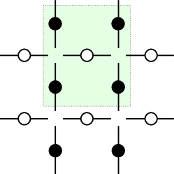
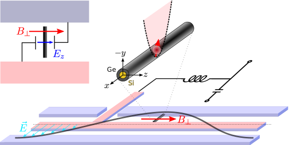
Figure S4: Left panel: schematics of the resonator-qubit lattice. Black and white dots represent qubits while straight lines represent microwave resonators. Right panel: Schematics of a CPW resonator with voltage biased center pin. The hole-spin qubit lives in a quantum dot formed in the wire either during growth or induced by additional gates (not shown). An electric field perpendicular to the wire is controlled by biasing the center conductor of the resonator. Furthermore, a magnetic field is applied in the plane of the resonators at an angle to the nanowires so as to generate a component perpendicular to all the nanowires.

Here we consider how to couple individual qubits together as required by the surface code. The resonator lattice system is depicted schematically in Fig. S4 (left panel). Note that because of the strong suppression of the $g$-factor along the axis of the nanowires Maier et al. (2013), we can neglect the component of the magnetic field along the nanowires. The magnetic field can be applied either perpendicular to the plane of the resonators or (preferably) in-plane. Here we focus on the latter situation. Hence each isolated site of the lattice is described by (S29).

We first focus on the Hamiltonian for the coupled resonators without the qubits. The novel feature here is the four-way capacitive coupling. A capacitor design which maximizes the capacitance between resonators at a right angle to each other and at the same times minimizes the direct capacitance across the junction is shown in Fig. S5 alongside with results from numerical finite element simulations, where we plot the different capacitances of the structure as a function of the capacitor lengths for varying channel widths. As this example illustrates, coupling capacitances on the order of a few tens of femto Farrads are feasible while achieving strong suppression of unwanted capacitances by more than two orders of magnitude.

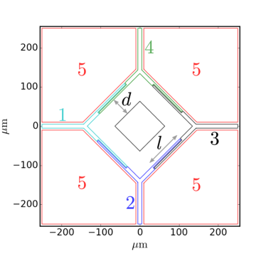
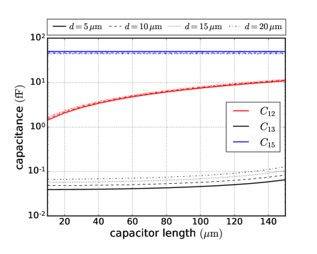
Figure S5: Capacitor design to maximize capacitive coupling between resonators at a right angle to each other while minimizing capacitive coupling directly across. Left panel: Four-way capacitor structure. right panel: Finite element simulation results.

Motivated by this we neglect the direct cross capacitance and model the coupling of one resonator to its four perpendicular neighbors (see Fig. 1 (g) of the main text) with the Lagrangian

$$\mathcal{L}=\frac{1}{2}\vec{\dot{\varphi}}^{T}\bm{C}\vec{\dot{\varphi}}-\frac{1}{2}\sum_{n=1}^{5}\frac{\varphi_{n}^{2}}{L}.$$ (S32)

Here we have modeled each isolated resonator mode as a single $LC$ resonance and $\varphi_{n}$ denotes the phase variable associated with the $n$-th resonator in units of the reduced flux quantum $\hbar/(2e)$. We have further introduced the real symmetric $5\times 5$ capacitance matrix $\bm{C}$. For a symmetric arrangement of equal cavities and denoting with $C$ the self capacitance of each center conductor and $C_{c}$ the pairwise coupling capacitances, the capacitance matrix reads

$$\bm{C}=\begin{pmatrix}C+4C_{c}&-C_{c}&-C_{c}&-C_{c}&-C_{c}\\ -C_{c}&C+4C_{c}&-C_{c}&-C_{c}&-C_{c}\\ -C_{c}&-C_{c}&C+4C_{c}&-C_{c}&-C_{c}\\ -C_{c}&-C_{c}&-C_{c}&C+4C_{c}&-C_{c}\\ -C_{c}&-C_{c}&-C_{c}&-C_{c}&C+4C_{c}\end{pmatrix}.$$ (S33)

The associated quantum Hamiltonian, obtained by canonical quantization is given by

$$\bm{H}_{5}=\omega_{r}\bm{a}_{n}^{\dagger}\bm{a}_{n}+J\left(\bm{a}_{n}^{\dagger}\bm{a}_{n-1}+\bm{a}_{n}^{\dagger}\bm{a}_{n+1}+\bm{a}_{n+1}^{\dagger}\bm{a}_{n}+\bm{a}_{n-1}^{\dagger}\bm{a}_{n}\right),$$ (S34)

with $\omega_{r}=1/\sqrt{L(C+4C_{c})}$ and $J=2\hbar\omega_{r}\frac{C_{c}}{C+4C_{c}}$.

The Hamiltonian for an entire square lattice of resonators with nearest neighbor capacitive coupling is then given by a straightforward generalization

$$\bm{H} =\omega_{r}\sum_{n,m=1}^{N}\bm{a}_{nm}^{\dagger}\bm{a}_{nm}+J\sum_{n,m}\left(\bm{a}_{nm}^{\dagger}\bm{a}_{nm+1}+\bm{a}_{nm}^{\dagger}\bm{a}_{nm-1}+\bm{a}_{nm}^{\dagger}\bm{a}_{n+1m}+\bm{a}_{nm}^{\dagger}\bm{a}_{n-1m}+{\rm h.c.}\right).$$ (S35)

Including the spin qubits and their coupling to the resonators immediately leads to the Jaynes-Cummings-Hubbard model (JCH) of Eq. (7) in the main text.

III Qubit gates

Here we provide further details on the single and two-qubit gates.

III.1 $R_{z}$ gate

A rotation of a selected qubit at lattice point $(n,m)$ around the $z$ axis can be achieved by exploiting the electric field dependence of the qubit frequency: If the perpendicular electric field in resonator at $(n,m)$ is tuned via the center pin to the working point $E_{z}^{*}$, then the qubit resonance frequency is decreased by an amount $\Delta\omega_{nm}=\omega_{Z}(E_{z}=0)-\omega_{Z}(E_{z}=E_{z}^{*})$. By simply waiting for a time $T$, a rotation $R_{z}(T\Delta\omega_{nm})$ around $z$ is induced. For the parameters given in the main text and a “on” field strength of $E_{z}^{*}=1\,{\rm V/\mu m}$ for example, $\Delta\omega_{nm}=1.161\times 2\pi\,{\rm GHz}$ which translates to a $\pi$ rotation around $z$ in a time $T_{\pi}\simeq 430\,{\rm ps}$.

III.2 Analytic fidelity upper bounds

In this section we derive the analytic upper bounds for the average fidelities of single and two-qubit gates given in the main text and shown in Fig. 3 (c) and (d) of the main text. We start with single qubit rotations. If the gate were perfect and the only source of imperfection were due to decoherence, then at zero temperature the single qubit density matrix would evolve as

$$\bm{\rho}(0)\rightarrow\bm{\rho}(T)=\begin{pmatrix}\rho_{ee}e^{-\gamma T}&\rho_{eg}e^{-\left(\frac{\gamma}{2}+\gamma_{\varphi}\right)T}\\ \rho_{ge}e^{-\left(\frac{\gamma}{2}+\gamma_{\varphi}\right)T}&1+(\rho_{gg}-1)e^{-\gamma T}\end{pmatrix},$$ (S36)

where $\rho_{ij}$ are the components of the initial state, $\gamma$ is the relaxation rate and $\gamma_{\varphi}$ the dephasing rate. The fidelity for a given initial state $\ket{\theta,\varphi}=\cos\left(\frac{\theta}{2}\right)\ket{0}+e^{i\varphi}\sin\left(\frac{\theta}{2}\right)\ket{1}$ on the Bloch sphere is given by

$$\mathcal{F}(\theta,\varphi)=\mathinner{\langle{\theta,\varphi|\bm{\rho}(t)|\theta,\varphi}\rangle}=\left(\sin^{4}(\theta/2)+\cos^{4}(\theta/2)\right)e^{-\gamma T}+2\sin^{2}(\theta/2)\cos^{2}(\theta/2)e^{-[\frac{\gamma}{2}+\gamma_{\varphi}]T}+\cos^{2}(\theta/2)(1-e^{-\gamma T}).$$ (S37)

Averaging over the Bloch sphere then yields

$$\mathcal{F}_{\varphi}=\frac{1}{4\pi}\int_{0}^{2\pi}d\varphi\int_{0}^{\pi}d\theta\sin(\theta)\mathcal{F}(\theta,\varphi)=\frac{1}{2}\left(1+\frac{1}{3}e^{-\gamma T}+\frac{2}{3}e^{-\left[\frac{\gamma}{2}+\gamma_{\varphi}\right]T}\right).$$ (S38)

Note that in our situation $T$ is the gate time, which is inversely proportional to the drive strength. Hence, $\gamma_{\varphi}$, which in our case is determined by photon shot noise, itself depends on $T$ (see Fig. 3 (c) of the main text).

For the two-qubit flip-flop gate we focus on a subset of initial states given by ${\rm span}\left\{\ket{eg},\ket{ge}\right\}$. The reason is that for a perfect gate, the flip-flop interaction acts trivially on both $\ket{gg}$ and $\ket{ee}$. The two states $\ket{eg}$ and $\ket{ge}$ span an effective Bloch sphere. Because these states live in the one excitation manifold, the fidelity of an ideal gate does in this case not depend on the angles $\theta$ and $\varphi$ and is thus simply given by $\mathcal{F}_{0}=e^{-\gamma T}$. Note that in this case we do not have photon induced dephasing to leading order since the resonator remains in the vacuum state.

IV Flip-flop interactions on the grid-bus lattice

Here we derive the effective flip-flop interaction between neighboring qubits on a $N\times M$ lattice of coupled resonators. It is convenient to introduce the Fourier modes

$$\bm{a}_{nm}=\frac{1}{\sqrt{NM}}\sum_{k=0}^{N-1}\sum_{l=0}^{M-1}e^{i\frac{2\pi k}{N}n}e^{i\frac{2\pi l}{N}m}\bm{b}_{kl},$$ (S39)

with $[\bm{b}_{kl},\bm{b}_{k^{\prime}l^{\prime}}^{\dagger}]=\delta_{kk^{\prime}}\delta_{ll^{\prime}}$, all other commutators being zero. In this basis, the JCH Hamiltonian reads

$$\bm{H} =\sum_{n,m}\frac{\omega_{nm}}{2}\bm{\sigma}_{nm}^{z}+\sum_{k,l}\left(\omega_{r}+2J\left[\cos\left(\frac{2\pi k}{N}\right)+\cos\left(\frac{2\pi l}{M}\right)\right]\right)\bm{b}_{kl}^{\dagger}\bm{b}_{kl}$$ (S40a)

$$+\frac{1}{\sqrt{NM}}\sum_{k,l}\sum_{n,m}\nu_{nm}\left(e^{i\frac{2\pi k}{N}n}e^{i\frac{2\pi l}{N}m}\bm{b}_{kl}\bm{\sigma}_{nm}^{+}+e^{-i\frac{2\pi k}{N}n}e^{-i\frac{2\pi l}{N}m}\bm{b}_{kl}^{\dagger}\bm{\sigma}_{nm}^{-}\right).$$ (S40b)

We next consider the dispersive regime. We define the anti-hermitian operator

$$\bm{S}=\frac{1}{\sqrt{NM}}\sum_{nm}\sum_{kl}\frac{\nu_{nm}}{\omega_{nm}-\omega_{r}-2J\left[\cos\left(\frac{2\pi k}{N}\right)+\cos\left(\frac{2\pi l}{M}\right)\right]}\left(e^{-i\frac{2\pi k}{N}n}e^{-i\frac{2\pi l}{M}m}\bm{\sigma}_{nm}^{-}\bm{b}_{kl}^{\dagger}-e^{i\frac{2\pi k}{N}n}e^{i\frac{2\pi l}{M}m}\bm{\sigma}_{nm}^{+}\bm{b}_{kl}\right).$$ (S41)

Splitting the Hamiltonian as $\bm{H}=\bm{H}_{0}+\bm{V}$, with $\bm{H}_{0}$ given by (S40a) and $V$ given by (S40b), we have

$$[\bm{H}_{0},\bm{S}]=-\bm{V}.$$ (S42)

In the dispersive regime of interest we have $|\omega_{nm}-\omega_{kl}|\gg\nu_{nm}$, where $\omega_{kl}=\omega_{r}+2J\left[\cos\left(\frac{2\pi k}{N}\right)+\cos\left(\frac{2\pi l}{M}\right)\right]$. The leading order correction to $\bm{H}_{0}$ upon performing the Schrieffer-Wolff transformation $\bm{H}\rightarrow e^{-\bm{S}}\bm{H}e^{\bm{S}}$, is given by $(1/2)[\bm{V},\bm{S}]$ where

$$[\bm{V},\bm{S}] =\frac{1}{NM}\sum_{nm,n^{\prime}m^{\prime}}\sum_{kl,k^{\prime}l^{\prime}}\left\{\frac{\nu_{nm}\nu_{n^{\prime}m^{\prime}}e^{i\frac{2\pi k}{N}n}e^{i\frac{2\pi l}{M}m}e^{-i\frac{2\pi k^{\prime}}{N}n^{\prime}}e^{-i\frac{2\pi l^{\prime}}{M}m^{\prime}}}{\omega_{n^{\prime}m^{\prime}}-\omega_{k^{\prime}l^{\prime}}}\left[\bm{b}_{kl}\bm{\sigma}_{nm}^{+},\bm{\sigma}_{n^{\prime}m^{\prime}}^{-}\bm{b}_{k^{\prime}l^{\prime}}^{\dagger}\right]\right\},$$ (S43a)

$$-\frac{1}{NM}\sum_{nm,n^{\prime}m^{\prime}}\sum_{kl,k^{\prime}l^{\prime}}\left\{\frac{\nu_{nm}\nu_{n^{\prime}m^{\prime}}e^{-i\frac{2\pi k}{N}n}e^{-i\frac{2\pi l}{M}m}e^{i\frac{2\pi k^{\prime}}{N}n^{\prime}}e^{i\frac{2\pi l^{\prime}}{M}m^{\prime}}}{\omega_{n^{\prime}m^{\prime}}-\omega_{k^{\prime}l^{\prime}}}\left[\bm{b}_{kl}^{\dagger}\bm{\sigma}_{nm}^{-},\bm{\sigma}_{n^{\prime}m^{\prime}}^{+}\bm{b}_{k^{\prime}l^{\prime}}\right]\right\}.$$ (S43b)

We further have

$$[\bm{b}_{kl}\bm{\sigma}_{nm}^{+},\bm{\sigma}_{n^{\prime}m^{\prime}}^{-}\bm{b}_{k^{\prime}l^{\prime}}^{\dagger}] =\delta_{nn^{\prime}}\delta_{mm^{\prime}}\bm{b}_{kl}\bm{b}_{k^{\prime}l^{\prime}}^{\dagger}\bm{\sigma}_{nm}^{z}+\delta_{kk^{\prime}}\delta_{ll^{\prime}}\bm{\sigma}_{nm}^{+}\bm{\sigma}_{n^{\prime}m^{\prime}}^{-},$$ (S44a)

$$[\bm{b}_{kl}^{\dagger}\bm{\sigma}_{nm}^{-},\bm{\sigma}_{n^{\prime}m^{\prime}}^{+}\bm{b}_{k^{\prime}l^{\prime}}] =-\delta_{nn^{\prime}}\delta_{mm^{\prime}}\bm{b}_{kl}^{\dagger}\bm{b}_{k^{\prime}l^{\prime}}\bm{\sigma}_{nm}^{z}-\delta_{kk^{\prime}}\delta_{ll^{\prime}}\bm{\sigma}_{nm}^{-}\bm{\sigma}_{n^{\prime}m^{\prime}}^{+}.$$ (S44b)

Substituting, we find after some algebra that the effective Hamiltonian can be written as

$$\bm{H}=\bm{H}_{0}+\bm{H}_{\rm L}+\bm{H}_{\rm d}+\bm{H}_{\rm nd}+\bm{H}_{XY},$$ (S45)

with

$$\bm{H}_{\rm L} =\frac{1}{2NM}\sum_{nm}\sum_{kl}\frac{\nu_{nm}^{2}}{\omega_{nm}-\omega_{kl}}\bm{\sigma}_{nm}^{z},$$ (S46a)

$$\bm{H}_{\rm d} =\frac{1}{NM}\sum_{nm}\sum_{kl}\frac{\nu_{nm}^{2}}{\omega_{nm}-\omega_{kl}}\bm{\sigma}_{nm}^{z}\bm{b}_{kl}^{\dagger}\bm{b}_{kl},$$ (S46b)

$$\bm{H}_{\rm nd} =\frac{1}{2NM}\sum_{nm}\sum_{k\not=k^{\prime},l\not=l^{\prime}}\frac{\nu_{nm}^{2}}{\omega_{nm}-\omega_{k^{\prime}l^{\prime}}}e^{i\frac{2\pi}{N}(k-k^{\prime})n}e^{i\frac{2\pi}{M}(l-l^{\prime})m}\bm{\sigma}_{nm}^{z}\bm{b}_{kl}\bm{b}_{k^{\prime}l^{\prime}}^{\dagger}+{\rm h.c.},$$ (S46c)

$$\bm{H}_{XY} =\frac{1}{NM}\sum_{nm,n^{\prime}m^{\prime}}\sum_{kl}\frac{\nu_{nm}\nu_{n^{\prime}m^{\prime}}}{\omega_{n^{\prime}m^{\prime}}-\omega_{kl}}e^{i\frac{2\pi}{N}k(n-n^{\prime})}e^{i\frac{2\pi}{M}l(m-m^{\prime})}\bm{\sigma}_{nm}^{+}\bm{\sigma}_{n^{\prime}m^{\prime}}^{-}+{\rm h.c.}$$ (S46d)

The first term (S46a) corresponds to a Lamb shift renormalization of the qubit frequencies. In the regime where $|\omega_{nm}-\omega_{r}|=|\Delta_{nm}|>4J$, the qubit frequency shift can be upper bounded as follows

$$|\Delta\omega_{nm}| =\left|\frac{\nu_{nm}^{2}}{NM\Delta_{nm}}\sum_{kl}\frac{1}{1-\frac{2J}{\Delta_{nm}}\left[\cos\left(\frac{2\pi k}{N}\right)+\cos\left(\frac{2\pi l}{M}\right)\right]}\right|$$ (S47)

$$=\left|\frac{\nu_{nm}^{2}}{NM\Delta_{nm}}\sum_{kl}\sum_{s=0}^{\infty}\left(\frac{2J}{\Delta_{nm}}\right)^{s}\left[\cos\left(\frac{2\pi}{N}k\right)+\cos\left(\frac{2\pi}{M}l\right)\right]^{s}\right|$$ (S48)

$$\leq\frac{\nu_{nm}^{2}}{|\Delta_{nm}|-4J}.$$ (S49)

The term $\bm{H}_{\rm d}$ corresponds to the dispersive interaction between the qubit and the eigenmodes of the coupled resonators. The term $\bm{H}_{\rm nd}$ corresponds to a qubit-state-dependent inter-eigenmode hopping term and finally, $\bm{H}_{XY}$ corresponds to a virtual photon mediated flip-flop interaction between qubit pairs.

IV.1 Coupling range in the weak coupling limit

We next elucidate the form of the two-qubit interaction and its range. For simplicity we consider the case of equal sub-systems such that $\nu_{nm}=\nu$, $\omega_{nm}=\omega_{Z}$. We further define $\Delta=\omega_{Z}-\omega_{r}$. Then the matrix elements of (S46d) are

$$K_{nm,n^{\prime}m^{\prime}}=\frac{1}{NM}\frac{\nu^{2}}{\Delta}\sum_{k,l}\frac{1}{1-\frac{2J}{\Delta}\left[\cos\left(\frac{2\pi k}{N}\right)+\cos\left(\frac{2\pi l}{M}\right)\right]}e^{i\frac{2\pi}{N}k(n-n^{\prime})}e^{i\frac{2\pi}{M}l(m-m^{\prime})}.$$ (S50)

We consider the weak coupling regime where $2J<|\Delta|$. Then resolving the geometric series we have

$$K_{nm,n^{\prime}m^{\prime}}=\frac{1}{NM}\frac{\nu^{2}}{\Delta}\sum_{k,l}\sum_{s=0}^{\infty}\left(\frac{2J}{\Delta}\right)^{s}\left[\cos\left(\frac{2\pi k}{N}\right)+\cos\left(\frac{2\pi l}{M}\right)\right]^{s}e^{i\frac{2\pi}{N}k(n-n^{\prime})}e^{i\frac{2\pi}{M}l(m-m^{\prime})}.$$ (S51)

Further using the binomial formula we obtain

$$K_{nm,n^{\prime}m^{\prime}}=\frac{1}{NM}\frac{\nu^{2}}{\Delta}\sum_{s=0}^{\infty}\sum_{q=0}^{s}\sum_{k,l}{{s}\choose{q}}\left(\frac{2J}{\Delta}\right)^{s}\cos^{q}\left(\frac{2\pi k}{N}\right)\cos^{s-q}\left(\frac{2\pi l}{M}\right)e^{i\frac{2\pi}{N}k(n-n^{\prime})}e^{i\frac{2\pi}{M}l(m-m^{\prime})}.$$ (S52)

Further writing $\cos(x)=(e^{ix}+e^{-ix})/2$ and applying the binomial formula twice more we find

$$K_{nm,n^{\prime}m^{\prime}} =\frac{1}{NM}\frac{\nu^{2}}{\Delta}\sum_{s=0}^{\infty}\sum_{q=0}^{s}\sum_{r=0}^{q}\sum_{t=0}^{s-q}\sum_{k,l}{{s}\choose{q}}{{q}\choose{r}}{{s-q}\choose{t}}\left(\frac{2J}{\Delta}\right)^{s}\frac{1}{2^{q}}\frac{1}{2^{s-q}}e^{\frac{2\pi ikr}{N}}e^{-\frac{2\pi ik(q-r)}{N}}e^{\frac{2\pi ilt}{M}}e^{-\frac{2\pi il(s-q-t)}{M}}e^{i\frac{2\pi}{N}k(n-n^{\prime})}e^{i\frac{2\pi}{M}l(m-m^{\prime})}$$ (S53)

$$=\frac{1}{NM}\frac{\nu^{2}}{\Delta}\sum_{s=0}^{\infty}\sum_{q=0}^{s}\sum_{r=0}^{q}\sum_{t=0}^{s-q}{{s}\choose{q}}{{q}\choose{r}}{{s-q}\choose{t}}\left(\frac{J}{\Delta}\right)^{s}\sum_{k,l}e^{\frac{2\pi i}{N}(2r-q+n-n^{\prime})k}e^{\frac{2\pi i}{M}(2t-s+q+m-m^{\prime})l}$$ (S54)

$$=\frac{\nu^{2}}{\Delta}\sum_{s=0}^{\infty}\sum_{q=0}^{s}\sum_{r=0}^{q}\sum_{t=0}^{s-q}\frac{s!}{r!(q-r)!t!(s-q-t)!}\left(\frac{J}{\Delta}\right)^{s}\delta_{2r-q+n-n^{\prime},0}\,\delta_{2t-s+q+m-m^{\prime},0}.$$ (S55)

To make further progress, we consider the different cases. Without restriction of generality we let $\Delta n=n-n^{\prime}\geq 0$ as well as $\Delta m=m-m^{\prime}\geq 0$. There are four possible cases:

• $\Delta n$ and $\Delta m$ even. Then the Kronecker deltas imply that only terms with even $q$ and even $s$ will contribute. Hence we set $s=2k$ and $q=2l$. We have

  $$K_{nm,n^{\prime}m^{\prime}} =\frac{\nu^{2}}{\Delta}\sum_{k=(\Delta m+\Delta n)/2}^{\infty}\sum_{l=\Delta n/2}^{k-\Delta m/2}\frac{(2k)!}{\left(l-\frac{\Delta n}{2}\right)!\left(l+\frac{\Delta n}{2}\right)!\left(k-l-\frac{\Delta m}{2}\right)!\left(k-l+\frac{\Delta m}{2}\right)!}\left(\frac{J}{\Delta}\right)^{2k}.$$ (S56)

• $\Delta n$ and $\Delta m$ odd. Then $q$ must be odd while $s$ must be even. Writing $s=2k$ and $q=2l+1$, we have

  $$K_{nm,n^{\prime}m^{\prime}} =\frac{\nu^{2}}{\Delta}\sum_{k=(\Delta m+\Delta n)/2}^{\infty}\sum_{l=(\Delta n-1)/2}^{k-(1+\Delta m)/2}\frac{(2k)!}{\left(l+\frac{1-\Delta n}{2}\right)!\left(l+\frac{1+\Delta n}{2}\right)!\left(k-l-\frac{1+\Delta m}{2}\right)!\left(k-l-\frac{1-\Delta m}{2}\right)!}\left(\frac{J}{\Delta}\right)^{2k}.$$ (S57)

• $\Delta n$ even and $\Delta m$ odd. Then $q$ must be even and $s$ must be odd. Writing $s=2k+1$ and $q=2l$ we have

  $$K_{nm,n^{\prime}m^{\prime}} =\frac{\nu^{2}}{\Delta}\sum_{k=(\Delta m+\Delta n-1)/2}^{\infty}\sum_{l=\Delta n/2}^{k+(1-\Delta m)/2}\frac{(2k+1)!}{\left(l-\frac{\Delta n}{2}\right)!\left(l+\frac{\Delta n}{2}\right)!\left(k-l+\frac{1-\Delta m}{2}\right)!\left(k-l+\frac{1+\Delta m}{2}\right)!}\left(\frac{J}{\Delta}\right)^{2k+1}.$$ (S58)

• $\Delta n$ odd and $\Delta m$ even. Then both $q$ and $s$ must be odd. Writing $q=2l+1$ and $s=2k+1$ we have

  $$K_{nm,n^{\prime}m^{\prime}} =\frac{\nu^{2}}{\Delta}\sum_{k=(\Delta m+\Delta n-1)/2}^{\infty}\sum_{l=(\Delta n-1)/2}^{k-\Delta m/2}\frac{(2k+1)!}{\left(l+\frac{1-\Delta n}{2}\right)!\left(l+\frac{1+\Delta n}{2}\right)!\left(k-l+\frac{1-\Delta m}{2}\right)!\left(k-l+\frac{1+\Delta m}{2}\right)!}\left(\frac{J}{\Delta}\right)^{2k+1}.$$ (S59)

In all four cases, when $J\ll\Delta$, the leading order term is

$$K_{nm,n^{\prime}m^{\prime}} =\frac{(\Delta m+\Delta n)!}{\Delta n!\Delta m!}\frac{\nu^{2}}{\Delta}\left(\frac{J}{\Delta}\right)^{\Delta m+\Delta n}.$$ (S60)

Hence to leading order, the coupling strength decays exponentially with the distance between the involved resonators as measured by $\Delta n+\Delta m=|n-n^{\prime}|+|m-m^{\prime}|$. By appropriately biasing the center conductors of adequate pairs of neighboring cavities, we can implement the pairwise two-qubit interactions between code and ancilla qubits required for the surface code. Note that, importantly, if we choose two different sets of frequencies for the white and black qubits illustrated in Fig. S4, we can realize these operations in parallel as explained in the main text (see also Fig. 2 in the main text).

To leading order, the qubit-qubit interaction is of the standard $XX+YY$ type:

$$\bm{H}_{XY}=\sum_{nn^{\prime},mm^{\prime}}K_{nn^{\prime},mm^{\prime}}\left(\bm{\sigma}_{nm}^{+}\bm{\sigma}_{n^{\prime}m^{\prime}}^{-}+\bm{\sigma}_{nm}^{+}\bm{\sigma}_{n^{\prime}m^{\prime}}^{-}\right)=\frac{1}{2}\sum_{nn^{\prime},mm^{\prime}}K_{nn^{\prime},mm^{\prime}}\left(\bm{\sigma}_{nm}^{x}\bm{\sigma}_{n^{\prime}m^{\prime}}^{x}+\bm{\sigma}_{nm}^{y}\bm{\sigma}_{n^{\prime}m^{\prime}}^{y}\right)$$ (S61)

For two qubits with equal couplings and frequencies, coupled to nearest neighbor lattices (either $m=m^{\prime}\pm 1$, $n=n^{\prime}$ or $n=n^{\prime}\pm 1$, $m=m^{\prime}$) the coupling strength is

$$K_{\rm NN}\simeq J\left(\frac{\nu}{\Delta}\right)^{2}.$$ (S62)

The XY interaction can be used to implement the $i{\rm SWAP}$ gate. Indeed, since $[\bm{X}\bm{X},\bm{Y}\bm{Y}]=0$ and $(\bm{X}\bm{X})^{2}=(\bm{Y}\bm{Y})^{2}=\openone_{2}\otimes\openone_{2}$, one has (setting $A=J_{\rm NN}/2$)

$$e^{-iAt(\bm{X}\bm{X}+\bm{Y}\bm{Y})} =e^{-iAt\bm{X}\bm{X}}e^{-iAt\bm{Y}\bm{Y}}=\left(\cos\left(At\right)-i\sin\left(At\right)\bm{X}\bm{X}\right)\left(\cos\left(At\right)-i\sin\left(At\right)\bm{Y}\bm{Y}\right)$$ (S63)

$$=\cos^{2}(At)+\sin^{2}(At)\bm{Z}\bm{Z}-i\sin(At)\cos(At)(\bm{X}\bm{X}+\bm{Y}\bm{Y}).$$ (S64)

Hence for $At=\pi/4$, we have the $i{\rm SWAP}$ gate

$$i{\rm SWAP}=\frac{1}{2}\left[\openone+\bm{Z}\bm{Z}-i(\bm{X}\bm{X}+\bm{Y}\bm{Y})\right]=\begin{pmatrix}1&0&0&0\\ 0&0&i&0\\ 0&i&0&0\\ 0&0&0&1\end{pmatrix}.$$ (S65)

The $\sqrt{i\rm SWAP}$ gate used in the main text is obtained simply by halving the evolution time. Together with single qubit rotations around an arbitrary axis, these gate forms a universal gate set. A CNOT gate for example can be obtained from single-qubit rotations and two $\sqrt{i\rm SWAP}$ gates Nielsen and Chuang (2000).

V Code folding

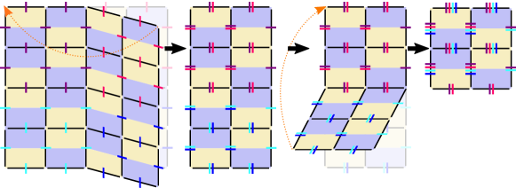
Figure S6: Code folding of a $40$ qubit lattice from one qubit per resonator to four and two qubits per resonator.

The small size of the qubits together with their tunable ac-field coupling offers the possibility to trade size with parallel processing capability: Instead of using one resonator per qubit as described above, each resonator hosts multiple qubits as depicted schematically in the rightmost panel of Fig. S6. The coupling of each qubit with the ac-field is now controlled by individual voltage bias lines. In the extreme case where an entire $2^{M}\times 2^{M}$ lattice is folded $M$ times onto a single square, all stabilizer mappings must be made sequentially because no more than one qubit per resonator can be coupled at a given time. Depending on the experimental situation however, a partial folding may provide the optimal compromise between size and speed.

VI Numerical simulations

This section provides further numerical results to complement those presented in the main text.

VI.1 Single-qubit rotation

Fig. S7 illustrates the time evolution of a $2\times 2$ lattice during the operation of a $\pi$ rotation around the $x$ axis of the qubit at lattice coordinate $(0,0)$. The same parameters are used as for Fig. 3 (c) of the main text. In particular the field applied to resonator at $(0,0)$ is $E_{z}=0.8\,{\rm V/\mu m}$. We can observe directly the small resonator population induced in the driven resonator as well as the effect of the drive on the adjacent resonators. The gate fidelity here is $98.7\%$.

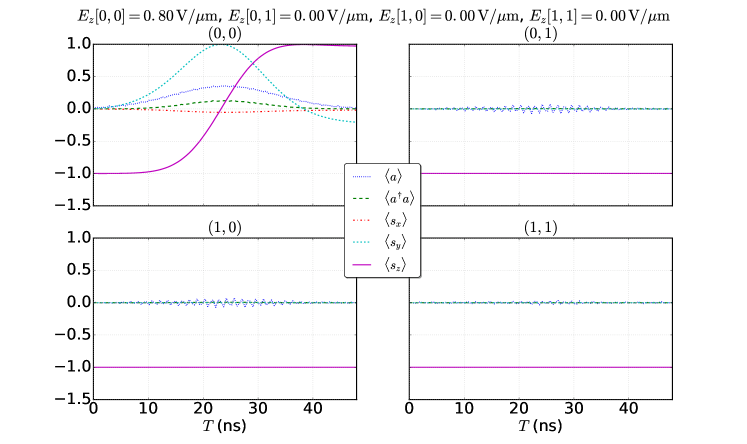
Figure S7: Time evolution in the rotating frame of a single-qubit rotation $R_{x}(\pi)$. The initial state is $\ket{gggg}$ in clock-wise ordering and only the first qubit is coupled to its cavity. The resonator population due to resonator-resonator coupling decreases the further the resonator is from the driven resonator.

VI.2 Two-qubit $\sqrt{i\rm SWAP}$ gate

Fig. S8 illustrates the time evolution of a $2\times 2$ lattice during the operation of a $\sqrt{i\rm SWAP}$ gate between qubits at lattice sites $(0,0)$ and $(0,1)$. The same parameters are used as in Fig. 3 (d) of the main text. A field of strength $E_{z}=0.9$ is applied to both resonators at $(0,0)$ and $(0,1)$. The gate fidelity here is $98.1\%$.

Figure S8: Time evolution of a two-qubit $\sqrt{i\rm SWAP}$ gate. The initial state is $\ket{gegg}$ in clock-wise ordering. The last two qubits are not coupled to their cavities and are seen to be unaffected by the gate.

References

• Taylor et al. (2005) J. M. Taylor, H.-A. Engel, W. Dur, A. Yacoby, C. M. Marcus, P. Zoller,  and M. D. Lukin, Nat Phys 1, 177 (2005).
• Chen et al. (2014) Y. Chen, C. Neill, P. Roushan, N. Leung, M. Fang, R. Barends, J. Kelly, B. Campbell, Z. Chen, B. Chiaro, A. Dunsworth, E. Jeffrey, A. Megrant, J. Y. Mutus, P. J. J. O’Malley, C. M. Quintana, D. Sank, A. Vainsencher, J. Wenner, T. C. White, M. R. Geller, A. N. Cleland,  and J. M. Martinis, Phys. Rev. Lett. 113, 220502 (2014).
• Nemoto et al. (2014) K. Nemoto, M. Trupke, S. J. Devitt, A. M. Stephens, B. Scharfenberger, K. Buczak, T. Nöbauer, M. S. Everitt, J. Schmiedmayer,  and W. J. Munro, Phys. Rev. X 4, 031022 (2014).
• Hill et al. (2015) C. D. Hill, E. Peretz, S. J. Hile, M. G. House, M. Fuechsle, S. Rogge, M. Y. Simmons,  and L. C. L. Hollenberg, Science Advances 1 (2015).
• Billangeon et al. (2015) P.-M. Billangeon, J. S. Tsai,  and Y. Nakamura, Phys. Rev. B 92, 020509 (2015).
• Brecht et al. (2016) T. Brecht, W. Pfaff, C. Wang, Y. Chu, L. Frunzio, M. H. Devoret,  and R. J. Schoelkopf, Npj Quantum Information 2, 16002 EP (2016).
• Karzig et al. (2016) T. Karzig, C. Knapp, R. Lutchyn, P. Bonderson, M. Hastings, C. Nayak, J. Alicea, K. Flensberg, S. Plugge, Y. Oreg, C. Marcus,  and M. H. Freedman, “Scalable designs for quasiparticle-poisoning-protected topological quantum computation with majorana zero modes,”  (2016), arXiv:1610.05289 .
• Bravyi and Kitaev (1998) S. Bravyi and A. Kitaev, “Quantum codes on a lattice with boundary,”  (1998), arXiv:quant-ph/9811052 .
• Helmer et al. (2009) F. Helmer, M. Mariantoni, A. G. Fowler, J. von Delft, E. Solano,  and F. Marquardt, EPL (Europhysics Letters) 85, 50007 (2009).
• DiVincenzo (2009) D. P. DiVincenzo, Physica Scripta 2009, 014020 (2009).
• Fowler et al. (2012) A. G. Fowler, M. Mariantoni, J. M. Martinis,  and A. N. Cleland, Phys. Rev. A 86, 032324 (2012).
• Barends et al. (2014) R. Barends, J. Kelly, A. Megrant, A. Veitia, D. Sank, E. Jeffrey, T. C. White, J. Mutus, A. G. Fowler, B. Campbell, Y. Chen, Z. Chen, B. Chiaro, A. Dunsworth, C. Neill, P. O/’Malley, P. Roushan, A. Vainsencher, J. Wenner, A. N. Korotkov, A. N. Cleland,  and J. M. Martinis, Nature 508, 500 (2014).
• Corcoles et al. (2015) A. D. Corcoles, E. Magesan, S. J. Srinivasan, A. W. Cross, M. Steffen, J. M. Gambetta,  and J. M. Chow, Nature Communications 6, 6979 EP (2015).
• Kelly et al. (2015) J. Kelly, R. Barends, A. G. Fowler, A. Megrant, E. Jeffrey, T. C. White, D. Sank, J. Y. Mutus, B. Campbell, Y. Chen, Z. Chen, B. Chiaro, A. Dunsworth, I.-C. Hoi, C. Neill, P. J. J. O/’Malley, C. Quintana, P. Roushan, A. Vainsencher, J. Wenner, A. N. Cleland,  and J. M. Martinis, Nature 519, 66 (2015).
• Takita et al. (2016) M. Takita, A. D. Córcoles, E. Magesan, B. Abdo, M. Brink, A. Cross, J. M. Chow,  and J. M. Gambetta, Phys. Rev. Lett. 117, 210505 (2016).
• Blais et al. (2004) A. Blais, R.-S. Huang, A. Wallraff, S. M. Girvin,  and R. J. Schoelkopf, Phys. Rev. A 69, 062320 (2004).
• Blais et al. (2007) A. Blais, J. Gambetta, A. Wallraff, D. I. Schuster, S. M. Girvin, M. H. Devoret,  and R. J. Schoelkopf, Phys. Rev. A 75, 032329 (2007).
• Majer et al. (2007) J. Majer, J. M. Chow, J. M. Gambetta, J. Koch, B. R. Johnson, J. A. Schreier, L. Frunzio1, D. I. Schuster, A. A. Houck, A. Wallraff, A. Blais, M. H. Devoret, S. M. Girvin,  and R. J. Schoelkopf1, Nature 449, 443 (2007).
• Gambetta et al. (2006) J. Gambetta, A. Blais, D. I. Schuster, A. Wallraff, L. Frunzio, J. Majer, M. H. Devoret, S. M. Girvin,  and R. J. Schoelkopf, Phys. Rev. A 74, 042318 (2006).
• Blumoff et al. (2016) J. Z. Blumoff, K. Chou, C. Shen, M. Reagor, C. Axline, R. T. Brierley, M. P. Silveri, C. Wang, B. Vlastakis, S. E. Nigg, L. Frunzio, M. H. Devoret, L. Jiang, S. M. Girvin,  and R. J. Schoelkopf, Phys. Rev. X 6, 031041 (2016).
• Gambetta et al. (2011) J. M. Gambetta, A. A. Houck,  and A. Blais, Phys. Rev. Lett. 106, 030502 (2011).
• Srinivasan et al. (2011) S. J. Srinivasan, A. J. Hoffman, J. M. Gambetta,  and A. A. Houck, Phys. Rev. Lett. 106, 083601 (2011).
• Eichler et al. (2015) C. Eichler, J. Mlynek, J. Butscher, P. Kurpiers, K. Hammerer, T. J. Osborne,  and A. Wallraff, Phys. Rev. X 5, 041044 (2015).
• Zhang et al. (2016) G. Zhang, Y. Liu, J. J. Raftery,  and A. A. Houck, “Suppression of photon shot noise dephasing in a tunable coupling superconducting qubit,”  (2016), arXiv:1603.01224 .
• Kloeffel et al. (2011) C. Kloeffel, M. Trif,  and D. Loss, Phys. Rev. B 84, 195314 (2011).
• Hu et al. (2012) Y. Hu, F. Kuemmeth, C. M. Lieber,  and C. M. Marcus, Nat Nano 7, 47 (2012).
• Kloeffel et al. (2013) C. Kloeffel, M. Trif, P. Stano,  and D. Loss, Phys. Rev. B 88, 241405 (2013).
• Prechtel et al. (2016) J. H. Prechtel, A. V. Kuhlmann, J. Houel, A. Ludwig, S. R. Valentin, A. D. Wieck,  and R. J. Warburton, Nat Mater 15, 981 (2016).
• Maurand et al. (2016) R. Maurand, X. Jehl, D. K. Patil, A. Corna, H. Bohuslavskyi, R. Laviéville, L. Hutin, S. Barraud, M. Vinet, M. Sanquer,  and S. D. Franceschi, “A cmos silicon spin qubit,”  (2016), arXiv:1605.07599 .
• Watzinger et al. (2016) H. Watzinger, C. Kloeffel, L. Vukusic, M. D. Rossell, V. Sessi, J. Kukucka, R. Kirchschlager, E. Lausecker, A. Truhlar, M. Glaser, A. Rastelli, A. Fuhrer, D. Loss,  and G. Katsaros, Nano Letters 16, 6879 (2016), pMID: 27656760, http://dx.doi.org/10.1021/acs.nanolett.6b02715 .
• Maier et al. (2014) F. Maier, J. Klinovaja,  and D. Loss, Phys. Rev. B 90, 195421 (2014).
• Flindt et al. (2006) C. Flindt, A. S. Sørensen,  and K. Flensberg, Phys. Rev. Lett. 97, 240501 (2006).
• Trif et al. (2007) M. Trif, V. N. Golovach,  and D. Loss, Phys. Rev. B 75, 085307 (2007).
• (34) See supplemental material at [URL provided by publisher].
• Samkharadze et al. (2016) N. Samkharadze, A. Bruno, P. Scarlino, G. Zheng, D. P. DiVincenzo, L. DiCarlo,  and L. M. K. Vandersypen, Phys. Rev. Applied 5, 044004 (2016).
• Maier et al. (2013) F. Maier, C. Kloeffel,  and D. Loss, Phys. Rev. B 87, 161305 (2013).
• Brauns et al. (2016) M. Brauns, J. Ridderbos, A. Li, E. P. A. M. Bakkers,  and F. A. Zwanenburg, Phys. Rev. B 93, 121408 (2016).
• Zhu et al. (2013) G. Zhu, S. Schmidt,  and J. Koch, New Journal of Physics 15, 115002 (2013).
• Koch et al. (2007) J. Koch, T. M. Yu, J. Gambetta, A. A. Houck, D. I. Schuster, J. Majer, A. Blais, M. H. Devoret, S. M. Girvin,  and R. J. Schoelkopf, Phys. Rev. A 76, 042319 (2007).
• Geerlings et al. (2013) K. Geerlings, Z. Leghtas, I. M. Pop, S. Shankar, L. Frunzio, R. J. Schoelkopf, M. Mirrahimi,  and M. H. Devoret, Phys. Rev. Lett. 110, 120501 (2013).
• Goppl et al. (2008) M. Goppl, A. Fragner, M. Baur, R. Bianchetti, S. Filipp, J. M. Fink, P. J. Leek, G. Puebla, L. Steffen,  and A. Wallraff, Journal of Applied Physics 104, 113904 (2008).
• Nielsen and Chuang (2000) M. A. Nielsen and I. L. Chuang, Quantum Computation and Quantum Information (Cambridge Univ. Press, 2000).
Supplementary Material for