Tensor perturbations during inflation in a spatially closed Universe

Abstract

In a recent paper [17], we studied the evolution of the background geometry and scalar perturbations in an inflationary, spatially closed Friedmann-Lemaître-Robertson-Walker (FLRW) model having constant positive spatial curvature and spatial topology $\mathbb{S}^{3}$. Due to the spatial curvature, the early phase of slow-roll inflation is modified, leading to suppression of power in the scalar power spectrum at large angular scales. In this paper, we extend the analysis to include tensor perturbations. We find that, similarly to the scalar perturbations, the tensor power spectrum also shows suppression for long wavelength modes. The correction to the tensor spectrum is limited to the very long wavelength modes, therefore the resulting observable CMB B-mode polarization spectrum remains practically the same as in the standard scenario with flat spatial sections. However, since both the tensor and scalar power spectra are modified, there are scale dependent corrections to the tensor-to-scalar ratio that leads to violation of the standard slow-roll consistency relation.

1 Introduction

Inflation is the leading paradigm of the early Universe, according to which the tiny temperature fluctuations observed in the cosmic microwave background (CMB) originate from quantum vacuum fluctuations at very early times [1, 2, 3, 4, 5, 6, 7]. One of the compelling features of the inflationary scenario is that it leads to an almost flat, homogeneous and isotropic Universe today starting from generic initial conditions. In particular, due to an exponential increases in the scale factor of the Universe, inflation dilutes away any effects of spatial curvature and as a result the spacetime is extremely well approximated by a spatially flat FLRW model at the end of inflation. Conversely, even though the spatial curvature effects are subdominant today, they could have been important in the early phases of inflation and in the pre-inflationary era. In addition, the equations of motion for cosmological perturbations include new curvature terms that become important at these times. In this scenario, modes of metric perturbations exiting the Hubble horizon at these early times can carry imprints of spatial curvature in their power spectrum.

Recent cosmological observations determine the density parameter due to the spatial curvature to be $\Omega_{\rm k}=-0.005_{-0.017}^{+0.016}$ from Planck data alone and $\Omega_{\rm k}=0.000_{-0.005}^{+0.005}$ by combining Planck measurements with BAO data [8]. While these values for $\Omega_{\rm k}$ are compatible with a flat FLRW model, they allow the possibility that our Universe is spatially closed with spatial topology of a 3-sphere ($\mathbb{S}^{3}$). For $\Omega_{\rm k}=-0.005$, the physical radius of this 3-sphere today is approximately $64~{}{\rm Gpc}$, which is $4.5$ times the physical radius of the CMB sphere. This indicates that the effects of the spatial curvature, if present, would be most prominent for length scales similar to or larger than that of the CMB sphere.

The presence of spatial curvature can affect observations in two ways: First, by affecting the background spacetime evolution in the post-inflationary era. This has been studied in detail by taking into account the consequences of spatial curvature on the Friedmann and Boltzmann equations in radiation and matter dominated era [9]. In this context, for a specified primordial power spectrum, the effect of $\mathbb{S}^{3}$ spatial topology during post-inflationary era on the CMB is numerically computed using the publically available code CAMB [9, 10]. Second, the spatial topology also introduces corrections to the primordial power spectrum of the scalar and tensor perturbations generated during inflation. This is the focus of the current and the accompanying paper [17]. Corrections to the primordial power spectrum of scalar perturbation due to $\mathbb{S}^{3}$ spatial topology have been previously studied using approximate methods [11, 12, 13, 14, 15, 16]. In the accompanying paper [17], we studied the evolution of the background geometry and gauge-invariant scalar perturbations in a spatially closed FLRW Universe where inflation is driven by a single scalar field in the presence of an inflationary potential (taken to be either quadratic or Starobinsky potential). We found that effects of non-vanishing spatial curvature become important during the early phases of inflation ($\sim 60$ e-folds before the end of inflation). Therefore, the long wavelength modes which exit the Hubble radius at those times can carry imprints of spatial curvature in their power spectrum. For both potentials, the resulting scalar power spectrum is different from the almost scale invariant power spectrum obtained in a spatially flat inflationary FLRW spacetime for long wavelength modes. In particular, the power spectrum shows oscillatory behavior that is most prominent for the long wavelength modes. In addition, there is suppression of power at such scales as compared to the flat model. For $\Omega_{\rm k}=-0.005$, the power deficit in the primordial power spectrum leads to suppression of power in the temperature anisotropy spectrum $C^{\rm TT}_{\ell}$ at $\ell<20$ [17]. For small wavelength modes, the power spectrum approaches the nearly scale invariant power spectrum and the resulting $C^{\rm TT}_{\ell}$ agrees extremely well with that in the flat model for $\ell\gtrsim 20$.

In every model of inflation, in addition to scalar fluctuations, the quantum vacuum fluctuations in the early Universe are also expected to generate tensor metric perturbations [18], which contribute to the B-mode polarization in the CMB. One of the main goals of the current and upcoming CMB experiments is the measurement and characterization of these primordial B-mode signals [19, 20, 21, 22]. Furthermore, the tensor perturbations generated during inflation give rise to primordial gravitational waves which are expected to contribute to the stochastic gravitational wave background at very low frequencies. Such low-frequency stochastic gravitational wave background can potentially be observed by space-based gravitational wave detectors such as eLISA [23, 24]. Since the primordial gravitational waves propagate through the Universe without being attenuated by the intermediate matter fields, they provide a direct window on the physics of the inflationary [25] as well as pre-inflationary era of the early Universe. Tensor perturbations have been studied in great detail in the context of spatially flat and open FLRW models [26, 27, 28, 29]. The goal of this paper is to investigate the effect of spatial curvature on the spectrum of primordial tensor perturbations generated during inflation in a spatially closed inflationary FLRW model as well as its effect on the B-mode polarization.

In this context we are led to the following questions: Scalar modes exiting the curvature radius during the early stages of inflation show power suppression. Is there similar suppression for tensor modes as well? If so, what effects does it produce in the CMB B-mode polarization signal and at what scales? One of the predictions of the single field slow-roll inflationary scenario is the so called slow-roll consistency relation that relates the tensor-to-scalar ratio $r$ with the tensor spectral index $n_{\rm t}$ [26, 28, 29]. This slow-roll consistency relation was derived for a flat FLRW model with Bunch-Davies initial conditions for the perturbations. Since the early slow-roll phase is modified in the closed model due to the presence of spatial curvature [17], it is natural to ask if the tensor-to-scalar ratio is also modified and whether or not the slow-roll consistency relation still holds true. The potential deviations from the standard slow-roll consistency relation, if measured by future experiments, can then be potentially used to refine the constraints on the spatial curvature of the Universe.

Our analysis shows that the tensor power spectrum is also suppressed at long wavelength scales, which is qualitatively similar to that in the scalar power spectrum. However, power is suppressed by a few percent for tensor perturbations as opposed to that for scalar perturbations in which case the suppression is as large as $10\%$ for the largest observable mode (corresponding to $\ell=2$) for $\Omega_{\rm k}=-0.005$. Due to the small suppression, the resulting B-mode polarization spectrum $C^{\rm BB}_{\ell}$ remains practically unchanged by the presence of positive spatial curvature. Since the scalar and tensor spectra are modified differently, the tensor-to-scalar ratio $r$ for a closed FLRW model is different from that for the flat model at long wavelength modes. Specifically, there is enhancement in $r$ at those scales. As a result, the slow-roll consistency relation is also modified for long wavelength modes. As shown in [17], short wavelength modes which exit the curvature radius later during inflation are not affected by the presence of spatial curvature. Therefore, $r$ and the slow-roll consistency relation for short wavelength modes for the spatially closed FLRW model are the same as that for the flat model.

The paper is organized as follows. In section 2.1, we provide a brief review of the evolution of the background spacetime for a spatially closed FLRW model. In section 2.2, we derive the equation of motion for tensor perturbations and discuss the choice of initial conditions. In section 3.1, we study the numerical evolution of tensor perturbations, compute the tensor primordial power spectrum, its impact on the B-mode polarization spectrum and compare the results with those for scalar modes. In section 3.2, we discuss the modifications in the tensor-to-scalar ratio and slow-roll consistency relation due to positive spatial curvature. We summarize the main results and discuss future outlook in section 4.

2 Spatially closed FLRW background geometry and tensor perturbations

This section is composed of two subsections. In section 2.1, we briefly revisit the equations governing the background geometry of a spatially closed FLRW model in the presence of an inflationary potential. In section 2.2, we will discuss the linear tensor metric perturbations $h_{ab}$ off the closed FLRW geometry. We will obtain the equations of motion of $h_{ab}$ and discuss the choice of initial conditions.

2.1 Background: dynamics and initial conditions

We consider a homogeneous, isotropic spatially curved FLRW model with topology $\mathbb{R}\times\mathbb{S}^{3}$ where $\mathbb{S}^{3}$ refers to the topology of the spatial sections. Choosing the scale factor today to be unity, i.e. $a_{0}=1$, the value of the curvature radius of the $\mathbb{S}^{3}$ spatial section $r_{o}$ can be expressed in terms of the Hubble constant $H_{0}$ and the spatial curvature parameter $\Omega_{\rm k}$ as $r_{o}=1/\sqrt{H_{0}^{2}|\Omega_{\rm k}|}$. With this convention, the spacetime metric is

$$ds^{2}=-dt^{2}+a^{2}(t)~{}r_{o}^{2}\,\left(d\chi^{2}+\sin^{2}\chi\,\left(d\theta^{2}+\sin^{2}\theta\,d\varphi^{2}\right)\right),$$ (2.1)

where $a(t)$ is the dimensionless scale factor. The unit 3-sphere on the spatial section $\mathbb{S}^{3}$ is coordinatized by $(\chi,\theta,\phi)$ which are defined in the domain: $\chi,\theta\in\left[0,\pi\right]$; $\phi\in\left[0,2\pi\right]$. In conformal time, defined by $dt=ad\eta$, the metric reads:

$$ds^{2}=a^{2}(\eta)\left[-d\eta^{2}+r_{o}^{2}\,\left(d\chi^{2}+\sin^{2}\chi\left(d\theta^{2}+\sin^{2}\theta\,d\varphi^{2}\right)\right)\right]\,.$$ (2.2)

The metric associated with the line element (2.2) can be written as $g_{ab}=a^{2}(\eta)\mathring{g}_{ab}$, where $\mathring{g}_{ab}$ describes a static metric with spherical spatial sections of radius $r_{o}$, that is, an Einstein Universe of radius $r_{o}$.

Given a matter field with energy density $\rho$, pressure $p$ and vanishing anisotropic stress, the dynamics of the background spacetime is governed by the Friedmann and Raychaudhuri equations:

$$H^{2} =\frac{8\pi G}{3}\rho-\frac{1}{a^{2}r_{o}^{2}},$$ (2.3)

$$\dot{H} =-4\pi G\left(\rho+p\right)+\frac{1}{a^{2}r_{o}^{2}},$$ (2.4)

where $H=\dot{a}/a$ is the Hubble parameter and ‘dot’ is used to represent the derivative with respect to proper time. Here we are interested in studying the dynamics of the background geometry during inflation in the presence of a single scalar field with a self-interacting potential $V(\phi)$. The energy density and pressure of the scalar field are then given by:

$$\rho=\frac{1}{2}\dot{\phi}^{2}+V(\phi)\qquad{\rm and}\qquad p=\frac{1}{2}\dot{\phi}^{2}-V(\phi).$$ (2.5)

Conservation of the energy momentum tensor of the scalar field results in the Klein-Gordon equation:

$$\ddot{\phi}+3H\dot{\phi}+\partial_{\phi}V(\phi)=0.$$ (2.6)

For a single field inflationary model, recent Planck data favors the Starobinsky potential over other potentials, therefore in this paper we will restrict our analysis to the Starobinsky potential:

$$V(\phi)=\frac{3m^{2}}{32\pi G}\left(1-e^{-\sqrt{\frac{16\pi G}{3}}\phi}\right)^{2}.\,$$ (2.7)

Nonetheless, the qualitative features of the results presented here also hold for other inflationary potentials. Specifically, the result that the power spectrum is modified for long wavelength can be attributed to the topology $\mathbb{S}^{3}$. However, the specifics of the modification and the scale at which the deviations from the scale invariant power spectrum appear depend on the interplay between the topology and the inflationary potential.

Usually, in the case of a spatially flat inflationary FLRW spacetime, the value of the mass parameter $m$ in eq. (2.7) is determined using the amplitude of the scalar power spectrum $A_{\rm s}$ and the associated spectral index $n_{\rm s}$ at the comoving pivot scale $k_{\star}$ from observations in conjunction with Einstein’s equations [37, 38, 39, 17]. This procedure also yields the values of $H$, $\phi$, $\dot{\phi}$ and $a$ (in the convention with $a_{0}=1$ today) at the time $t=t_{\star}$, i.e. when the pivot mode $k_{\star}$ exits the Hubble radius during inflation. Here, we will use the data from the Planck mission for which amplitude of the scalar power spectrum $A_{\rm s}=(2.2065\pm 0.0035)\times 10^{-9}$ and scalar spectral index $n_{\rm s}=0.9645\pm 0.0049$ at the pivot scale $k_{\star}=0.05~{}{\rm Mpc^{-1}}$. In principle, for a closed FLRW model, the values of various parameters at $t=t_{\star}$ would be different from that in the flat model and one would need to re-compute them. However, it turns out that at $t=t_{\star}$ the ratio of the total energy density due to the spatial curvature and that due to the inflaton field remains smaller than $10^{-6}$ for the range of $\Omega_{\rm k}$ given by Planck measurements. Therefore, the conditions at $t_{\star}$ are practically the same as those in the spatially flat FLRW model [17]. We obtain the following conditions at $t=t_{\star}$:

$$a_{\star} = (2.11\pm 0.14)\times 10^{-53},\qquad\quad\;\;\phi_{\star}=1.06\pm 0.057~{}m_{\rm Pl},$$

$$H_{\star} = (1.25\pm 0.32)\times 10^{-6}~{}m_{\rm Pl}^{2},\qquad\dot{\phi}_{\star}=(-5.27\pm 3.18)\times 10^{-9}m_{\rm Pl}^{2},$$ (2.8)

where subscript ‘$\star$’ indicates that the quantities are evaluated at horizon exit time $t=t_{\star}$. The mass parameter is

$$m=(2.67\pm 0.18)\times 10^{-6}~{}m_{\rm Pl}.$$ (2.9)

As shown in Fig. 1, the effects of $\Omega_{\rm k}$ become important approximately 8 e-folds before $t_{\star}$.

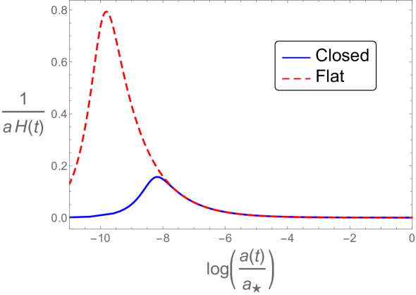
Figure 1: Comoving Hubble horizon $(aH)^{-1}$ plotted with respect to the number of e-folds from the horizon exit time $t_{\star}$ of the pivot mode. The dashed (red) and the solid (blue) curves correspond to spatially flat and closed models respectively. It is evident that the spatial curvature starts becoming important approximately 8 e-folds before $t_{\star}$. The onset of accelerated expansion marked by $\ddot{a}=0$—which corresponds to the maximum of the curves—happens approximately 10 e-folds before $t_{\star}$ in the flat model and apprximately 8 e-folds before $t_{\star}$ in the closed model.

Within the range of allowed conditions at $t_{\star}$, the condition that maximize the effect of spatial curvature corresponds to the situation for which the size of the comoving wavelength of the largest observable mode is comparable to the comoving Hubble horizon $(aH)^{-1}$ at the onset of inflation. This initial condition will be contrasted to the initial condition corresponding to the best fit value of the parameters $A_{\rm s}$ and $n_{\rm s}$ in the results in the next section. Specifically, for the ‘maximal effect’ condition we have:

$$\phi_{\star}=1.02~{}m_{\rm Pl},\qquad\dot{\phi}_{\star}=-6.69\times 10^{-9}m_{\rm Pl}^{2}.$$ (2.10)

The evolution of the background spacetime after the end of inflation, which is marked by $\epsilon:=-\dot{H}/H^{2}=1$, is governed by the $\Lambda{\rm CDM}~{}$model. We will assume instantaneous reheating and will use $\Omega_{\rm m}=0.31,~{}\Omega_{\rm r}=9.2\times 10^{-5},~{}\Omega_{\rm\Lambda}=0.69$ as determined by Planck. For the spatial curvature, we work with $\Omega_{\rm k}=-0.005$ as a representative value to show plots and discuss numerical results.

2.2 Tensor perturbations: dynamics and initial conditions

We introduce linear perturbations on the FLRW background with spherical spatial surfaces described in the previous section by splitting the metric into a background and a perturbation part. Specifically, we consider a one-parameter family of metrics $g_{ab}(\varepsilon)$:

$$g_{ab}(\varepsilon)=a^{2}(\eta)\left(\mathring{g}_{ab}+\varepsilon h_{ab}\right)\,,$$ (2.11)

where $a^{2}\mathring{g}_{ab}$ is the background metric (2.2), $h_{ab}$ is a linear perturbation and $\varepsilon$ is a smallness parameter. Indices of the perturbation $h_{ab}$ are raised and lowered with $\mathring{g}_{ab}$ and its inverse $\mathring{g}^{ab}$. Since we are interested only in the tensor components of $h_{ab}$, we can focus on its transverse traceless part $h_{ab}^{TT}$, that is,

$$h_{ab}^{TT}\eta^{b}=0,\qquad\qquad\mathring{\nabla}^{a}h_{ab}^{TT}=0\qquad{\rm and}\qquad\mathring{g}^{ab}h_{ab}^{TT}=0,$$

with $\eta^{a}$ the globally time-like conformal Killing vector field of the background metric $\mathring{g}^{ab}$ and $\mathring{\nabla}_{a}$ the derivative operator compatible with $\mathring{g}_{ab}$. The equations of motion of the tensor perturbations are then obtained by linearizing Einstein’s equations. For the nonvanishing spatial components, we find:

$$\mathring{\nabla}^{2}h_{ij}^{TT}-2\frac{a^{\prime}}{a}h_{ij}^{{}^{\prime}\,TT}-\frac{2}{r_{o}^{2}}h_{ij}^{TT}=0\,,$$ (2.13)

where the ‘prime’ denotes the partial derivative with respect to conformal time $\eta$ and $i,j=1,2,3$ denote spatial indices. Note that although we have used a specific background, this equation is true for any FLRW model with matter field(s) having vanishing anisotropic stress.

Recall that in the case of flat spatial sections, instead of solving the equations of motion in real space, one expands the perturbations into their Fourier modes. The equations of motion then become an ordinary differential equation for each Fourier mode. Similarly, in the spatially closed model considered here, it is convenient to expand the perturbations in a basis spanned by the tensor hyperspherical harmonics $\mathcal{Q}^{nlm,s}_{ij}(\chi,\theta,\phi)$ [41]. Let $\gamma_{ij}$ be the metric of the three-sphere $\mathbb{S}^{3}$ with radius $r_{o}$ and $D_{i}$ the corresponding covariant derivative. These hyperspherical harmonics are tensor eigenfunctions of the Laplacian operator $D^{2}$:

$$D^{2}\mathcal{Q}^{nlm,s}_{ij}(\chi,\theta,\phi)=-\frac{(n^{2}-3)}{r_{o}^{2}}\mathcal{Q}^{nlm,s}_{ij}(\chi,\theta,\phi)\,,$$ (2.14)

satisfying

$$\gamma^{ij}\,\mathcal{Q}^{nlm,s}_{ij}=0\,,\qquad D^{i}\mathcal{Q}^{nlm,s}_{ij}=0\,,$$

and form an orthonormal basis in the space of transverse traceless tensor fields on $\mathbb{S}^{3}$. They are labelled by integers in the intervals: $n\geq 3$, $l\in[0,n-1]$, $m\in[-l,l]$. The polarization index $s$ assumes values $s=0,1$, which distinguish between even and odd harmonics with respect to the parity operator

$$P_{2}(\chi,\theta,\varphi)=(\chi,\pi-\theta,\pi+\phi)\,,$$ (2.15)

i.e., $\mathcal{Q}^{nlm,s}_{ij}\left(P_{2}(\chi,\theta,\varphi)\right)=(-1)^{l+s}\mathcal{Q}^{nlm,s}_{ij}(\chi,\theta,\varphi)$. For an explicit expression of these tensor hyperspherical harmonics and their derivation, see [41, 42]. The factor $(n^{2}-3)/r_{o}^{2}$ can be interpreted as the curved version of the wavenumber squared ($k^{2}$) by analogy with the flat model for which the eigenfunctions of the flat space Laplacian have eigenvalue $-k^{2}$ [9].

We expand the tensor perturbations in terms of the tensor hyperspherical harmonics as follows:

$$h_{ij}^{TT}(\eta,\chi,\theta,\phi)=\sum_{s}\sum_{nlm}h^{s}_{nlm}(\eta)\mathcal{Q}^{nlm,s}_{ij}(\chi,\theta,\phi),$$ (2.16)

All dynamical information of $h_{ab}^{TT}$ is now encoded in the amplitudes $h^{s}_{nlm}(\eta)$ which are purely functions of time. Substituting this decomposition into eq. (2.13) yields the following equation of motion for $h^{s}_{nlm}$:

$$h^{s~{}^{\prime\prime}}_{nlm}+2\frac{a^{\prime}}{a}h^{s~{}^{\prime}}_{nlm}+\left(\frac{n^{2}-3}{r_{o}^{2}}+\frac{2}{r_{o}^{2}}\right)h^{s}_{nlm}=0\,.$$ (2.17)

Introducing the variable $\mu^{s}_{nlm}(\eta)=a(\eta)h^{s}_{nlm}(\eta)$, we obtain:

$$\mu^{s~{}^{\prime\prime}}_{nlm}+\left(\frac{n^{2}-1}{r_{o}^{2}}-\frac{a^{{}^{\prime\prime}}}{a}\right)\mu^{s}_{nlm}=0\,.$$ (2.18)

The field $\hat{\mu}^{s}_{nlm}(\eta)$ behaves like a scalar field and can be written in the standard Fock representation as follows:

$$\hat{\mu}^{s}_{nlm}(\eta)=\hat{A}_{nlm}^{s}~{}e_{nlm}^{s}(\eta)+{\hat{A}_{nlm}}^{s~{}\dagger}~{}{e^{s\,\star}_{nlm}}(\eta).$$ (2.19)

Here, $\hat{A}^{s~{}\dagger}_{nlm}$ and $\hat{A}^{s}_{nlm}$ are the creation and annihilation operators and the mode functions $e_{nlm}^{s}(\eta)$ form the positive frequency basis. Since the two polarizations denoted by the superscript ‘$s$’ evolve independently, in the following we will drop this superscript for notational clarity. The mode functions then satisfy the following equations of motion:

$$e^{{}^{\prime\prime}}_{nlm}+\left(\frac{n^{2}-1}{r_{o}^{2}}-\frac{a^{{}^{\prime\prime}}}{a}\right)e_{nlm}=0\,.$$ (2.20)

The normalization condition for $e_{nlm}$ is

$$e_{nlm}e^{\star\prime}_{nlm}-e^{\prime}_{nlm}e^{\star}_{nlm}=i~{}.$$ (2.21)

The choice of the vacuum state $|0\rangle$ annihilated by $\hat{A}_{nlm}$ is associated with the choice of the positive frequency basis $e_{nlm}$. Recall that in a static FLRW Universe (i.e. a Universe for which $a(t)$ is constant), the vacuum state can be uniquely selected by requiring it to be regular and invariant under all spatial symmetries and time-translations. This state then automatically minimizes the Hamiltonian for tensor perturbations. For a dynamical, time-dependent background such as the FLRW model considered here, there is no such state that minimizes the Hamiltonian at all times. In order to compare our results with those for the spatially flat scenario, we work with an instantaneous vacuum state. This state is defined by the basis function $e_{nlm}$ that minimizes the Hamiltonian for the perturbations at a given time $\eta_{\rm ini}$ [43, 44]. The basis mode functions for this instantaneous vacuum are:

$$e_{nlm}(\eta_{\rm ini}) = \frac{1}{\sqrt{2\omega_{n}\,r_{o}}}\,,$$

$${e}^{\prime}_{nlm}(\eta_{\rm ini}) = -i\sqrt{\frac{\omega_{n}}{2\,r_{o}}}\,$$ (2.22)

with $\omega_{n}=\sqrt{\frac{n^{2}-1}{r_{o}^{2}}-\frac{a^{{}^{\prime\prime}}}{a}}$ [17]. The initial conditions are given at the onset of inflation defined by $\ddot{a}=0$.

Since the Hamiltonian is minimized at an instant of time, the vacuum state chosen here depends on the time at which the initial conditions are specified. Nevertheless, the time dependence of the instantaneous vacuum state chosen is weak for all observable modes. This is because for the initial conditions for the background spacetime all observable modes are within the curvature radius at the initial time $\eta_{\rm ini}$. As a result, the initial state for the perturbations is nearly static close to the onset of inflation. In the numerical evolution of the modes, we explicitly verified this.

Remarks:
(i) In the standard inflationary scenario with spatially flat sections, the initial states for quantum perturbations representing scalar and tensor perturbations are often chosen to be the Bunch-Davies vacuum state at a time when all obervable modes are inside the curvature radius and the spacetime can be well approximated by a de Sitter spacetime. From Fig. 1 it is clear that, 8 e-folds before $t_{\star}$ when all observable modes can safely be assumed to be within the Hubble horizon, the flat model is still well approximated by a quasi-de Sitter spacetime. Therefore, it is safe to assume that all modes are in the Bunch-Davies state 8 or more e-folds before $t_{\star}$. This is no longer true in the closed model. As shown in Fig. 1, the spatial curvature becomes important at those times and the spacetime is no longer quasi-de Sitter. Therefore, it is not justifiable to take the quantum perturbations in the Bunch-Davies vacuum state. Moreover, the spacetime is dynamical and the symmetries of the spacetime are not enough to select a unique vacuum state unlike in the de Sitter spacetime. There remains a large freedom in the choice of initial state. As discussed above, in this paper, we choose an instantaneous vacuum state at the time when $\ddot{a}=0$ for the quantum perturbations. This choice is adopted for both the flat and closed models for the comparison of the predicted power spectra, in order to isolate effects due to the presence of spatial curvature from those related to the choice of the initial vacuum.

(ii) For observable modes, the static vacuum chosen here also satisfies the WKB approximation. If we had chosen the instantaneous state at a time before $\ddot{a}=0$ when the slow-roll and WKB approximations are both violated, then the power spectrum of the long wavelength modes would change while that for the short, ultraviolet modes would remain the same as that in the flat model.

(iii) In this paper, we have taken the topology of the homogeneous, spatial slices to be $\mathbb{S}^{3}$. This is the simplest topology compatible with a constant positive spatial curvature in three-dimensions, and provides a natural framework for the analysis of effects due to the deviation from spatially flat geometry. The local geometry does not fix the global topology uniquely, however, and our results can be extended to various other topologies compatible with a locally spherical geometry. Signatures of a nontrivial topology in the temperature and polarization CMB spectra have been heavily studied for flat and open spatial sections (see for instance, [45, 46]), and a family of spherical spaces – specifically lens and prism spaces – has been studied in [47, 48] for which the mathematical and numerical groundwork was laid in [49, 50]. The allowed global metrics compatible with a locally spherically symmetric geometry were classified in [51], and have the generic form $\mathbb{S}^{3}/\Gamma$, where $\Gamma$ is a subgroup of isometries of $\mathbb{S}^{3}$ acting freely and discontinuously. The topology is modified through the identification of points on $\mathbb{S}^{3}$ related by the action of elements of $\Gamma$, and an infinite number of topologies can be constructed in this way, falling in a small number of classes [52]. For example, take the simplest nontrivial topology one can build this way: the projective space, $RP^{3}=\mathbb{S}^{3}/\mathbb{Z}_{2}$, which is obtained by identifying antipodal points. Given a point on the sphere with coordinates $(\chi,\theta,\phi)$, the cosmological parity operator ${P}_{3}$ relates antipodal points:

$${P}_{3}=\begin{cases}\chi\to\pi-\chi,\\ \theta\to\pi-\theta,\\ \phi\to\pi+\phi\,.\end{cases}$$ (2.23)

Since antipodal points are identified for the construction of $RP^{3}$, only modes with the same value at antipodal points contribute. In other words, only those hyperspherical harmonics with $n$ odd are present in $RP^{3}$. Since at the linearized level all modes evolve independently, this does not alter their dynamics and hence the resulting primordial power spectrum is not affected for the odd modes while all even modes are forced to vanish. If one goes beyond the linearized level, modes will couple and this is no longer true.

(iv) As a side observation, for a spatially flat Universe, taking the massless limit in the equation of motion for the scalar modes yields the equation of motion for the tensor modes. This is not true for a Universe with closed spatial topology.

3 Results

This section is divided into two subsections. In the first, we will calculate the tensor power spectrum at the end of inflation and the resulting B-mode polarization spectrum in the CMB. In the second subsection, we will discuss the violation of the slow-roll consistency relation due to the spatial curvature. Recall from section 1 that the presence of the nonvanishing spatial curvature can affect observations in two distinct ways. First, by introducing corrections to the Friedmann equations and equations of motion of the perturbations during inflation. As shown in [17], the energy density due to spatial curvature becomes important during the early stages of inflation. As a result, although the background geometry of a spatially closed inflationary FLRW spacetime at the end of inflation is indistinguishable from a spatially flat FLRW spacetime, the modes of quantum fields representing scalar and tensor metric perturbations, which exit the curvature radius during early times can carry imprints of spatial curvature in their power spectrum. The second effect of the spatial curvature is due to the fact that in $\mathbb{S}^{3}$ topology the wavenumbers of the quantum perturbations are discrete rather than a continuum as in the flat model. This effect becomes important in the post-inflationary era in the computation of the anisotropy spectrum in the CMB by solving the Boltzmann equations starting from an initial condition at the end of inflation. Only a finite number of discrete modes contribute to the temperature anisotropy observed in the CMB and the final expression of $C_{\ell}$ is a discrete sum over the modes rather than an integral. As shown in [17] the aggregate effect for the scalar modes was suppression in the temperature anisotropy spectrum $C^{\rm TT}_{\ell}$ in the CMB at multipoles $\ell<20$. As we will see in this section, the tensor modes also show deficit of power at those scales, but the percentage suppression is much smaller than that for scalar modes for the same background inflationary solution. For the discussion of the results, we will use the initial conditions for the background perturbations as described in the previous sections with $\Omega_{\rm k}=-0.005$.

3.1 Primordial power spectrum and B-mode polarization spectrum

In order to study the power spectrum of the quantum perturbations we numerically solve the equation of motion subject to the initial conditions discussed in section 2. We work with the canonical representation for the scalar ($v$) and tensor ($\mu$) perturbations which are governed by the following equations of motion. For scalar modes:

$$\ddot{v}_{n}(t)+b^{(S)}(n,t)~{}\dot{v}_{n}(t)+c^{(S)}(n,t)~{}v_{n}(t)=0,$$ (3.1)

and for tensor modes

$$\ddot{\mu}_{n}(t)+b^{(T)}(n,t)~{}\dot{\mu}_{n}(t)+c^{(T)}(n,t)~{}\mu_{n}(t)=0,$$ (3.2)

where

$$b^{(S)}(n,t)=H+\frac{32\pi Ga^{3}\dot{a}\dot{\phi}V^{\prime}(\phi)+48\pi Ga^{2}\dot{a}^{2}\dot{\phi}^{2}-8\pi Ga^{2}\dot{\phi}^{2}\left(8\pi Ga^{2}\left(\dot{\phi}^{2}-2V\right)+2\right)}{2a\dot{a}\left(2(n^{2}-4)\dot{a}^{2}+8\pi Ga^{2}\dot{\phi}^{2}\right)}~{},$$ (3.3)

$$c^{(S)}(n,t)=\frac{8\pi G}{a^{2}\dot{a}^{2}\left(2\left(n^{2}-4\right)\dot{a}^{2}+8\pi Ga^{2}\dot{\phi}^{2}\right)}\\ \Bigg{[}\frac{\dot{a}^{4}(n^{2}-4)\left(n^{2}-1+a^{2}V^{\prime\prime}\right)}{4\pi G}+\left(4n^{2}-7\right)a^{3}\dot{a}^{3}\dot{\phi}V^{\prime}-\pi G\frac{n^{2}-1}{n^{2}-4}a^{4}\dot{\phi}^{4}\left[8\pi Ga^{2}\left(\dot{\phi}^{2}+2V\right)-6\right]\\ +(n^{2}-1)a^{2}\dot{a}^{2}\Bigg{(}-6\pi G\frac{n^{2}-5}{n^{2}-4}a^{2}\dot{\phi}^{4}+4\pi Ga^{2}\dot{\phi}^{2}V+\frac{3}{2}\dot{\phi}^{2}+\frac{9}{2}\dot{a}^{2}\dot{\phi}^{2}\Bigg{)}\\ +a^{3}\dot{a}\left[a\dot{a}\dot{\phi}^{2}V^{\prime\prime}+2a\dot{a}V^{\prime 2}+4\pi Ga^{2}\dot{\phi}V^{\prime}\left(\dot{\phi}^{2}+2V\right)-\dot{\phi}V^{\prime}\right]\Bigg{]}-H~{}b^{(S)}(n,t)-\frac{\ddot{a}}{a}~{},$$ (3.4)

$$b^{(T)}(n,t)=H~{},$$ (3.5)

and

$$c^{(T)}(n,t)=\frac{n^{2}-1}{r_{o}^{2}~{}a^{2}}-H^{2}-\frac{\ddot{a}}{a}.$$ (3.6)

Here, we have written the equations in cosmic time which is what is used for the numerical evolution of the modes. For notational convenience we have dropped the sub- and superscripts denoting spherical wavenumbers and polarization for the tensor modes.

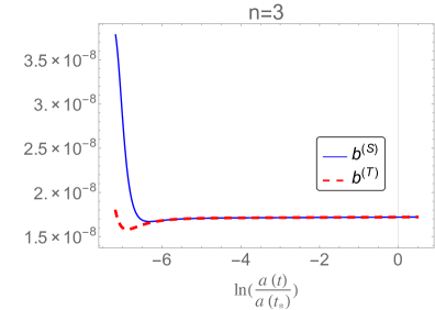
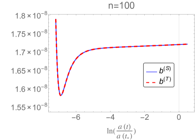
Figure 2: Friction terms for scalar and tensor modes plotted for $n=3$ (left panel) and $n=100$ (right panel) with respect to the number of e-folds from the time when the pivot modes exits the horizon during slow-roll. It is evident that $b^{(S)}$ and $b^{(T)}$ differ from each other for $n=3$ at early times while they are practically the same for $n=100$.

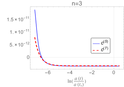
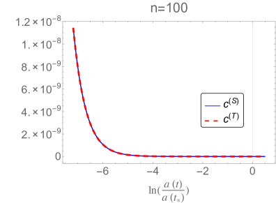
Figure 3: Potential terms for scalar and tensor modes plotted for $n=3$ (left panel) and $n=100$ (right panel) with respect to the number of e-folds from the time when the pivot modes exits the horizon during slow-roll. As was the case for the friction terms in Fig. 2, $c^{(S)}$ and $c^{(T)}$ differ from each other for $n=3$ at early times while they are practically the same for $n=100$.

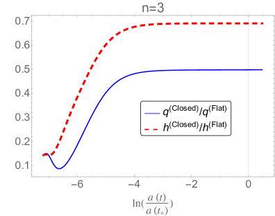
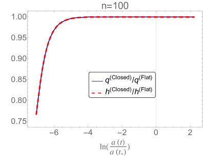
Figure 4: Evolution of scalar and tensor modes for spatially closed FLRW model with $\Omega_{\rm k}=-0.005$. For the clarity of presentation we have plotted $q=v/a$ and $h=\mu/a$. It is evident that the two modes evolve differently for $n=3$ but in a very similar way for $n=100$. In particular the amplitude of the scalar modes is lower than that of the tensor modes for $n=3$ after they have exited the horizon during inflation.

These equations are similar to that of a damped harmonic oscillator where $b^{(S)}$ and $b^{(T)}$ act like friction and $c^{(S)}$ and $c^{(T)}$ play the role of time dependent potential. Figures 2 and 3 respectively show the evolution of the friction and potential terms for scalar and tensor perturbations. In both figures the left panels correspond to the longest wavelength mode with $n=3$ and the right panels correspond to the mode with $n=100$. It is evident that both friction and potential terms are different for the tensor and scalar modes for $n=3$, while they are practially the same for the scalar and tensor modes for $n=100$. That is, for small $n$, the presence of spatial curvature affects the evolution of tensor and scalar modes quantiatively differently. For large $n$, however, since both the friction and potential terms for scalar and tensor modes are indistinguishable from each other the evolution of tensor and scalar modes is very similar. This behavior is apparent in Fig. 4. The scalar mode with $n=3$ evolves differently from the tensor one and has a lower amplitude after the horizon exit. Whereas, for $n=100$ both the scalar and the tensor modes have the same amplitude. This indicates that in a spatially closed FLRW model, there is a scale dependent correction to the power spectra of the tensor and scalar perturbations.

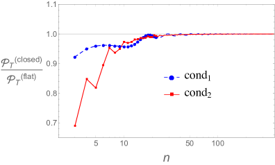
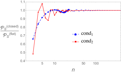
Figure 5: Left panel: Ratio of the tensor power spectrum in the closed FLRW model with $\Omega_{\rm k}=-0.005$ to that in the flat model. Right panel: Ratio of the scalar power spectrum in the closed FLRW model with $\Omega_{\rm k}=-0.005$ to that in the flat model. Both spectra show suppression of power at small $n$. However, the scalar modes are significantly more suppressed in the closed Universe as compared to the tensor modes. The two curves in each figure correspond to two different initial conditions for the background geometry: ‘${\rm cond}_{1}$’ corresponds to eq. (2.8) (matching with the best fit values for $A_{\rm s}$ and $n_{\rm s}$ at $t_{\star}$) and ‘${\rm cond}_{2}$’ corresponds to eq. (2.10) (generating maximal suppression). In both figures the spectra are discrete in $n$ (for clarity discrete points are shown only for $n<20$).

The left panel of Fig. 5 shows the ratio of the tensor power spectrum at the end of inflation in the closed FLRW model with $\Omega_{\rm k}=-0.005$ to that in the flat FLRW model with $\Omega_{\rm k}=0$. The ratio approaches unity for modes with large $n$ describing the short wavelength modes which exit the curvature radius later during inflation. At these times the effect of spatial curvature on the evolution of both the background and perturbations is negligible and the background spacetime can be very well approximated by a quasi-de Sitter spacetime. For small $n$, which correspond to long wavelength modes, however, the ratio is smaller than unity. That is, the tensor power spectrum is suppressed in the spatially closed model compared to the spatially flat model for these modes. As the figure shows, there is as much as 5-30% suppression in power for modes with $n<10$. The scalar power spectrum (shown in the right panel of Fig. 5), for the spatially closed FLRW model also shows suppression for modes with small $n$ and approaches that for the flat model as $n$ increases. For the same inflationary background geometry, the suppression in the scalar power spectrum is larger and is as large as 15% for $n=10$ and 50% for $n=3$.

Hence, the presence of spatial curvature modifies the background geometry and the evolution of the quantum metric perturbations in such a way that the power is suppressed for both the tensor and scalar models at long wavelength modes. However, there are differences in the percentage suppressions in tensor and scalar modes. This is quite different from power suppression mechanisms proposed in the spatially flat FLRW model by either envisaging a fast roll phase prior to the onset of the usual slow-roll phase [53, 54, 55, 56, 31] or by considering excited initial states which may arise due to some pre-inflationary physics [30]. In those proposals, the relative change to both power spectra (tensor and scalar) are very similar to each other, unlike what we find in Fig. 5 for the spatially closed FLRW model.

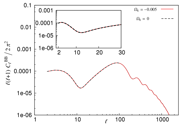
Figure 6: The B-mode polarization spectrum $C^{\rm BB}_{\ell}$ in the CMB for $\Omega_{\rm k}=-0.005$ (solid red curve) and $\Omega_{\rm k}=0$ (black dashed curve). In spite of the differences in the tensor primordial power spectrum (Fig. 5) at low $n$, the observable $C^{\rm BB}_{\ell}$ remains practically unchanged in the presence of the spatial curvature for $\Omega_{\rm k}=-0.005$ with initial conditions corresponding to ${\rm cond}_{2}$ for which the wavelength of the largest observable mode is comparable to the Hubble horizon at the onset of inflation.

Let us now discuss how the CMB B-mode polarization spectrum is affected due to the modifications in the tensor primordial spectrum shown in Fig. 5. We use the publicly available Boltzmann solver CAMB [9, 10] to evolve the primordial power spectrum until the surface of last scattering and compute the resulting $C^{\rm BB}_{\ell}$ shown in Fig. 6. As the figure shows, the resulting $C^{\rm BB}_{\ell}$ for $\Omega_{\rm k}=-0.005$ is practically indistinguishable from that in the spatially flat model (with $\Omega_{\rm k}=0$). This happens because the corrections to the tensor primordial power spectrum is limited to very low wavenumbers ($n<15$), which correspond to super-horizon modes. This is true not only for initial conditions corresponding to the best fit values of $A_{\rm s}$ and $n_{\rm s}$ (${\rm cond}_{1}$), but also for the initial conditions that generate maximal suppression of power in the primordial tensor power spectrum (${\rm cond}_{2}$). Thus, this result is robust under changing the initial conditions for the background.

Remark: If one considers the coupling between long and short wavelength modes along the lines of [57, 58, 59, 60, 61], the corrections to the primordial power spectrum at small $n$ could influence the computation of super-horizon modulation to the observed two-point function for both tensor and scalar modes depending on the type of coupling considered.

3.2 Tensor-to-scalar ratio and the slow-roll consistency relation

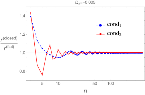
Figure 7: The tensor-to-scalar ratio $r$ in the spatially closed model compared with that in the flat model. For small $n$, which correspond to modes exiting the Hubble horizon at early times during inflation, $r$ in the closed model is modified compared to the flat model. For large $n$ modes, which exit the Hubble horizon later during inflation, $r$ in the closed model is practically the same as in the flat model. As in Fig. 5, ${\rm cond}_{1}$ and ${\rm cond}_{2}$ correspond to the background initial conditions eq. (2.8) and (2.10) respectively.

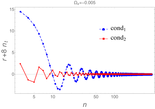
Figure 8: The deviation from the consistency relation ($r+8n_{\rm t}=0$) for $\Omega_{\rm k}=-0.005$ plotted with respect to the spherical wavenumber $n$. It is evident that for small $n$ deviation from $r+8n_{\rm t}=0$ is more prominent. These deviations approach zero as $n$ increases. As before, ${\rm cond}_{1}$ and ${\rm cond}_{2}$ respectively correspond to the background initial conditions eq. (2.8) and (2.10) respectively.

As shown in Fig. 5, the modifications to the tensor and scalar power spectrum for a spatially closed model are different quantitatively. Therefore, the tensor-to-scalar ratio $r$ also shows deviation from the predictions of the standard inflationary scenario for a flat FLRW model. Fig. 7 shows the ratio of $r$ in the closed FLRW model with $\Omega_{\rm k}=-0.005$ to that in the flat FLRW model. In each figure the dashed (blue) and the solid (red) curves correspond to initial conditions given in eq. (2.8) and eq. (2.10) respectively. As discussed previously in this section, the effect of the spatial curvature on the evolution of the modes with large $n$ is minimal. Therefore, the ratio $r^{\rm(closed)}/r^{\rm(flat)}$ approaches unity for large $n$. However, both the scalar and tensor power spectra are modified and as a result the tensor-to-scalar ratio for the closed model shows deviation from the flat model for small $n$. The differences are most prominent for modes with $n<10$ which correspond to super horizon modes for $\Omega_{\rm k}=-0.005$. So, as far as the observable modes are concerned, the correction to $r$ due to the spatial curvature is small.

Let us now understand the impact of spatial curvature on the slow-roll consistency relation. One of the important features of the standard slow-roll inflation in a flat FLRW model, assuming Bunch-Davies initial conditions for the perturbations, is the relation between $r$ and tensor spectral index $n_{\rm t}$: $r^{\rm(flat)}\approx-8n_{\rm t}$, where ‘$\approx$’ indicates that the relation is valid only in the slow-roll approximation. This relation is known as the slow-roll consistency relation and it holds regardless of the choice of potential and hence can be used as test of the standard inflationary scenario. In the scenario considered here, $r$ acquires scale dependent modifications due to the non-zero spatial curvature (see Fig. 7). So, one is naturally led to ask: Is the consistency relation also modified? Fig. 8 shows the behavior of $r+8n_{\rm t}$ (which is zero for the standard scenario) in the presence of spatial curvature. It is evident from the figure that at large $n$ the consistency relation holds just as in the standard case, while for small $n$ there are deviations for the closed model.

4 Summary and outlook

One of the attractive features of the inflationary scenario is that it ‘dilutes’ away the information about the spatial curvature. The CMB observations confirm this by putting strong constraints on the spatial curvature ($\Omega_{\rm k}$) today. During inflation, the contribution from the spatial curvature to the total curvature of the spacetime goes as $a^{-2}$ while that from the scalar field remains almost constant. Therefore, even if the spatial curvature of the spacetime was important before the onset of inflation, it becomes negligible with respect to the energy density of the matter field within a few e-folds. As a result, the spacetime is extremely well approximated by a flat FLRW model at the end of inflation and in the post-inflationary era. This suggests that while most of the inflationary and post-inflationary evolution of the spacetime remains unaffected by the spatial curvature, the early phases of inflation can be modified by a non-vanishing $\Omega_{\rm k}$. In that case, long wavelength modes which exit the Hubble horizon at these early times can carry imprints of spatial curvature in their power spectrum. In a recent paper [17], we considered the evolution of gauge-invariant scalar perturbations in a spatially closed FLRW model and found that the primordial scalar power spectrum is indeed modified leading to suppression of power at large angular scales in the CMB temperature anisotropy spectrum $C^{\rm TT}_{\ell}$.

In this paper, we extended the analysis to include tensor modes. Similarly to the scalar perturbations, the tensor power spectrum is modified due to the presence of closed spatial curvature for modes with small $n$ that exit the curvature radius at early phases of inflation. For these modes, the power in the primordial tensor spectrum is suppressed compared to that in the flat inflationary FLRW spacetime. However, we find that the relative suppression for tensor modes is smaller than that for the scalar modes. The suppression in the tensor power spectrum is weak and limited to very small $n$, which correspond to super-horizon modes. Consequently, the resulting observable polarization anisotropy spectrum $C^{\rm BB}_{\ell}$ in closed FLRW model differs less than a percent from the flat FLRW model. Since the tensor and scalar spectra are modified differently by the spatial curvature, the tensor-to-scalar ratio at the long wavelength modes acquires scale dependent corrections which further leads to the violation of the standard slow-roll consistency relation obtained for the flat FLRW model. Hence, although the modifications in the tensor spectrum due to closed spatial curvature do not have a direct observable imprint in the B-mode polarization signal, they lead to violation of the standard slow-roll consistency relation for long wavelength modes. This deviation from the standard relation, if observed, can be used to further refine the constraints on spatial curvature of the Universe.

Since the effects of spatial curvature is more dominant in the early phases of inflation, it is expected that the pre-inflationary dynamics of the spacetime and its Planck scale behavior in the presence of closed spatial curvature will be different from the spatially flat model. A priori, it is not clear if inflation will even happen if one provides initial conditions in the deep Planck regime. These issues have been investigated in the setting of loop quantum cosmology (LQC) for the spatially flat FLRW model [63, 64, 65, 30, 38, 39]. It is expected that the interplay between the quantum gravity corrections due to LQC and the spatial curvature may bring out interesting features that could be relevant for observations. In future work [66], we will study the Planck dynamics of the closed FLRW spacetime using the LQC framework developed in [67], and study the evolution of quantum perturbations on the quantum modified background geometry.

We considered spacetimes with spatial sections isometric to the three-sphere $\mathbb{S}^{3}$, the simplest global geometry compatible with a constant positive spatial curvature. The local geometry constrains the global topology but does not fix it uniquely. In this work, we focused on the analysis of geometric effects due to the presence of spatial curvature, but our framework can also be applied to the study of observational signatures of the spatial topology in locally spherically Universes. In particular, solutions for the equations of motion for tensor perturbations on nontrivial topologies can always be written as linear superpositions of normal modes on $\mathbb{S}^{3}$, allowing the evolution of perturbations and the primordial power spectrum to be determined for arbitrary topologies from the results herein discussed for the dynamics of the perturbations on $\mathbb{S}^{3}$.

5 Acknowledgements

We are grateful to Abhay Ashtekar for discussions. BB would also like to thank Steve Carlip and Glenn Starkman for discussions on the topology of the Universe. This work was supported by NSF grant PHY-1505411 and the Eberly research funds of Penn State. BB is grateful for receiving a Mebus Fellowship and NY acknowledges support from CNPq, Brazil. This work used the Extreme Science and Engineering Discovery Environment (XSEDE), which is supported by National Science Foundation grant number ACI-1053575.

References

- [1] A. H. Guth, “The Inflationary Universe: A Possible Solution to the Horizon and Flatness Problems”, Phys.Rev. D23 (1981) 347–356.
- [2] A. Albrecht and P. J. Steinhardt, “Cosmology for Grand Unified Theories with Radiatively Induced Symmetry Breaking”, Phys.Rev.Lett. 48 (1982) 1220–1223.
- [3] A. D. Linde, “A New Inflationary Universe Scenario: A Possible Solution of the Horizon, Flatness, Homogeneity, Isotropy and Primordial Monopole Problems”, Phys.Lett. B108 (1982) 389–393.
- [4] A. D. Linde, “Chaotic Inflation”, Phys.Lett. B129 (1983) 177–181.
- [5] A. R. Liddle and D. Lyth, “Cosmological inflation and large scale structure”, Cambridge University Press, 2000.
- [6] V. Mukhanov, “Physical foundations of cosmology”, Cambridge University Press, 2005.
- [7] S. Weinberg, “Cosmology”, Oxford University Press, Oxford, 2008.
- [8] Planck Collaboration, P. A. R. Ade et al., “Planck 2015 results. XIII. Cosmological parameters”, Astron. Astrophys. 594 (2016) A13, arXiv:1502.01589.
- [9] A. Lewis, A. Challinor, and A. Lasenby, “Efficient computation of CMB anisotropies in closed FRW models”, Astrophys. J. 538 (2000) 473–476, astro-ph/9911177.
- [10] A. Lewis, “CAMB Notes”, http://cosmologist.info/notes/CAMB.pdf
- [11] J.-P. Uzan, U. Kirchner, and G. F. R. Ellis, “WMAP data and the curvature of space”, Mon. Not. Roy. Astron. Soc. 344 (2003) L65, arXiv:astro-ph/0302597.
- [12] G. F. R. Ellis, S. J. Stoeger, William R., P. McEwan, and P. Dunsby, “Dynamics of inflationary universes with positive spatial curvature”, Gen. Rel. Grav. 34 (2002)a 1445–1459, arXiv:gr-qc/0109023.
- [13] G. F. R. Ellis, P. McEwan, S. J. Stoeger, William R., and P. Dunsby, “Causality in inflationary universes with positive spatial curvature”, Gen. Rel. Grav. 34 (2002)b 1461–1481, arXiv:gr-qc/0109024.
- [14] G. Efstathiou, “Is the low CMB quadrupole a signature of spatial curvature?”, Mon. Not. Roy. Astron. Soc. 343 (2003) L95, arXiv:astro-ph/0303127.
- [15] A. Lasenby and C. Doran, “Closed universes, de Sitter space and inflation”, Phys. Rev. D71 (2005) 063502, arXiv:astro-ph/0307311.
- [16] J. P. Luminet, J. Weeks, A. Riazuelo, R. Lehoucq, and J. P. Uzan, “Dodecahedral space topology as an explanation for weak wide - angle temperature correlations in the cosmic microwave background”, Nature 425 (2003) 593, arXiv:astro-ph/0310253.
- [17] B. Bonga, B. Gupt, and N. Yokomizo, “Inflation in the closed FLRW model and the CMB”, JCAP 1610 (2016), no. 10, 031, arXiv:1605.07556.
- [18] A. A. Starobinsky, “Spectrum of relic gravitational radiation and the early state of the universe”, JETP Lett. 30 (1979) 682–685, [Pisma Zh. Eksp. Teor. Fiz.30,719(1979)].
- [19] SPTpol Collaboration, D. Hanson et al., “Detection of B-mode Polarization in the Cosmic Microwave Background with Data from the South Pole Telescope”, Phys. Rev. Lett. 111 (2013), no. 14, 141301, arXiv:1307.5830.
- [20] BICEP2 Collaboration, P. A. R. Ade et al., “Detection of -Mode Polarization at Degree Angular Scales by BICEP2”, Phys. Rev. Lett. 112 (2014)a, no. 24, 241101, arXiv:1403.3985.
- [21] POLARBEAR Collaboration, P. A. R. Ade et al., “A Measurement of the Cosmic Microwave Background B-Mode Polarization Power Spectrum at Sub-Degree Scales with POLARBEAR”, Astrophys. J. 794 (2014)b, no. 2, 171, arXiv:1403.2369.
- [22] D. J. Watts et al., “Measuring the Largest Angular Scale CMB B-mode Polarization with Galactic Foregrounds on a Cut Sky”, Astrophys. J. 814 (2015), no. 2, 103, arXiv:1508.00017.
- [23] P. Amaro-Seoane et al., “eLISA/NGO: Astrophysics and cosmology in the gravitational-wave millihertz regime”, GW Notes 6 (2013) 4–110, arXiv:1201.3621.
- [24] N. Bartolo et al., “Science with the space-based interferometer LISA. IV: Probing inflation with gravitational waves”, arXiv:1610.06481.
- [25] M. Zaldarriaga and U. Seljak, “Gravitational lensing effect on cosmic microwave background polarization”, Phys. Rev. D58 (1998) 023003, arXiv:astro-ph/9803150.
- [26] V. F. Mukhanov, H. A. Feldman, and R. H. Brandenberger, “Theory of cosmological perturbations.”, Phys. Rept. 215 (1992) 203–333.
- [27] M. S. Turner, M. J. White, and J. E. Lidsey, “Tensor perturbations in inflationary models as a probe of cosmology”, Phys. Rev. D48 (1993) 4613–4622, arXiv:astro-ph/9306029.
- [28] J. E. Lidsey, A. R. Liddle, E. W. Kolb, E. J. Copeland, T. Barreiro, and M. Abney, “Reconstructing the inflation potential : An overview”, Rev. Mod. Phys. 69 (1997) 373–410, arXiv:astro-ph/9508078.
- [29] D. Baumann, “Inflation”, in “Physics of the large and the small, TASI 09, proceedings of the Theoretical Advanced Study Institute in Elementary Particle Physics, Boulder, Colorado, USA, 1-26 June 2009”, pp. 523–686. 2011. arXiv:0907.5424.
- [30] I. Agullo, A. Ashtekar, and W. Nelson, “The pre-inflationary dynamics of loop quantum cosmology: Confronting quantum gravity with observations”, Class. Quant. Grav. 30 (2013) 085014, arXiv:1302.0254.
- [31] L. Lello, D. Boyanovsky, and R. Holman, “Pre-slow roll initial conditions: large scale power suppression and infrared aspects during inflation”, Phys. Rev. D89 (2014) 063533, arXiv:1307.4066.
- [32] J. D. Barrow and S. Cotsakis, “Inflation and the Conformal Structure of Higher Order Gravity Theories”, Phys. Lett. B214 (1988) 515–518.
- [33] K.-i. Maeda, “Towards the Einstein-Hilbert Action via Conformal Transformation”, Phys. Rev. D39 (1989) 3159.
- [34] A. A. Starobinsky, S. Tsujikawa, and J. Yokoyama, “Cosmological perturbations from multifield inflation in generalized Einstein theories”, Nucl. Phys. B610 (2001) 383–410, arXiv:astro-ph/0107555.
- [35] A. De Felice and S. Tsujikawa, “f(R) theories”, Living Rev. Rel. 13 (2010) 3, arXiv:1002.4928.
- [36] Planck Collaboration, P. A. R. Ade et al., “Planck 2015 results. XX. Constraints on inflation”, Astron. Astrophys. 594 (2016) A20, arXiv:1502.02114.
- [37] A. Ashtekar and B. Gupt, “Quantum gravity in the sky: interplay between fundamental theory and observations”, Classical and Quantum Gravity 34 (2017), no. 1, 014002, arXiv:1608.0422.
- [38] B. Bonga and B. Gupt, “Inflation with the Starobinsky potential in Loop Quantum Cosmology,” Gen. Rel. Grav. 48, no. 6, 71 (2016) arXiv:1510.00680.
- [39] B. Bonga and B. Gupt, “Phenomenological investigation of a quantum gravity extension of inflation with the Starobinsky potential”, Phys. Rev. D93 (2016), no. 6, 063513, arXiv:1510.04896.
- [40] R. M. Wald, “General Relativity,” Chicago, Usa: Univ. Pr. ( 1984) 491p
- [41] U. H. Gerlach and U. K. Sengupta, “Homogeneous Collapsing Star: Tensor and Vector Harmonics for Matter and Field Asymmetries”, Phys. Rev. D18 (1978) 1773–1784.
- [42] A. Challinor, “Microwave background polarization in cosmological models”, Phys. Rev. D62 (2000) 043004, arXiv:astro-ph/9911481.
- [43] V. Mukhanov and S. Winitzki, “Introduction to quantum effects in gravity”, Cambridge University Press, 2007.
- [44] S. A. Fulling, “Aspects of Quantum Field Theory in Curved Space-time”, London Math. Soc. Student Texts 17 (1989) 1–315.
- [45] N. J. Cornish, D. N. Spergel and G. D. Starkman, “Circles in the Sky: Finding Topology with the Microwave Background Radiation,” Class. Quant. Grav. 15, 2657 (1998)
- [46] O. Fabre, S. Prunet and J. P. Uzan, “Topology beyond the horizon: how far can it be probed?,” Phys. Rev. D 92, no. 4, 043003 (2015)
- [47] J. P. Uzan, A. Riazuelo, R. Lehoucq and J. Weeks, “Cosmic microwave background constraints on lens spaces,” Phys. Rev. D 69, 043003 (2004) arXiv:astro-ph/0303580.
- [48] A. Riazuelo, J. P. Uzan, R. Lehoucq and J. Weeks, “Simulating cosmic microwave background maps in multi-connected spaces,” Phys. Rev. D 69, 103514 (2004) arXiv:astro-ph/0212223.
- [49] R. Lehoucq, J. Weeks, J. P. Uzan, E. Gausmann and J. P. Luminet, “Eigenmodes of three-dimensional spherical spaces and their application to cosmology,” Class. Quant. Grav. 19, 4683 (2002) arXiv:gr-qc/0205009.
- [50] R. Lehoucq, J. P. Uzan, and J. Weeks, “Eigenmodes of lens and prism spaces,” Kodai Mathematical Journal 26, (2003)
- [51] H. Seifert and W. Threlfall, Math. Ann. 104, 1 (1934), English transl. by M.A. Goldman, “A textbook on topology”, New York: Academic Press (1980)
- [52] M. Lachiéze-Rey and J-P. Luminet, “Cosmic topology,” Phys. Rept. 254, 135 (1995)
- [53] C. R. Contaldi, M. Peloso, L. Kofman, and A. D. Linde, “Suppressing the lower multipoles in the CMB anisotropies”, JCAP 0307 (2003) 002, arXiv:astro-ph/0303636.
- [54] J. M. Cline, P. Crotty and J. Lesgourgues, “Does the small CMB quadrupole moment suggest new physics?,” JCAP 0309 (2003) 010 arXiv:astro-ph/0304558
- [55] R. K. Jain, P. Chingangbam, J.-O. Gong, L. Sriramkumar, and T. Souradeep, “Punctuated inflation and the low CMB multipoles”, JCAP 0901 (2009) 009, arXiv:0809.3915.
- [56] F. G. Pedro and A. Westphal, “Low- CMB power loss in string inflation”, JHEP 04 (2014) 034, arXiv:1309.3413.
- [57] A. L. Erickcek, S. M. Carroll, and M. Kamionkowski, “Superhorizon Perturbations and the Cosmic Microwave Background”, Phys. Rev. D78 (2008)a 083012, arXiv:0808.1570.
- [58] A. L. Erickcek, M. Kamionkowski, and S. M. Carroll, “A Hemispherical Power Asymmetry from Inflation”, Phys. Rev. D78 (2008)b 123520, arXiv:0806.0377.
- [59] F. Schmidt and L. Hui, “Cosmic Microwave Background Power Asymmetry from Non-Gaussian Modulation”, Phys. Rev. Lett. 110 (2013) 011301, arXiv:1210.2965, [Erratum: Phys. Rev. Lett.110,059902(2013)].
- [60] I. Agullo, “Loop quantum cosmology, non-Gaussianity, and CMB power asymmetry”, Phys. Rev. D92 (2015) 064038, arXiv:1507.04703.
- [61] S. Adhikari, S. Shandera, and A. L. Erickcek, “Large-scale anomalies in the cosmic microwave background as signatures of non-Gaussianity”, Phys. Rev. D93 (2016), no. 2, 023524, arXiv:1508.06489.
- [62] A. Ashoorioon, J. L. Hovdebo and R. B. Mann, “Running of the spectral index and violation of the consistency relation between tensor and scalar spectra from trans-Planckian physics,” Nucl. Phys. B 727, 63 (2005) gr-qc/0504135
- [63] A. Ashtekar and D. Sloan, “Probability of Inflation in Loop Quantum Cosmology,” Gen. Rel. Grav. 43, 3619 (2011) arXiv:1103.2475.
- [64] A. Ashtekar and D. Sloan, “Loop quantum cosmology and slow roll inflation,” Phys. Lett. B 694, 108 (2011) arXiv:0912.4093.
- [65] A. Corichi and A. Karami, “On the measure problem in slow roll inflation and loop quantum cosmology,” Phys. Rev. D 83, 104006 (2011) arXiv:1011.4249.
- [66] B. Bonga, B. Gupt, and N. Yokomizo, in preparation
- [67] A. Ashtekar, T. Pawlowski, P. Singh and K. Vandersloot, “Loop quantum cosmology of k=1 FRW models,” Phys. Rev. D 75, 024035 (2007) arXiv:0612104.