A global model of cylindrical and coaxial surface-wave discharges

Abstract

A volume-averaged global model is developed to investigate surface-wave discharges inside either cylindrical or coaxial structures. The neutral and ion wall flux is self-consistently estimated based on a simplified analytical description both for electropositive and electronegative plasmas. The simulation results are compared with experimental data from various discharge setups of either argon or oxygen, measured or obtained from literature, for a continuous and a pulse-modulated power input. A good agreement is observed between the simulations and the measurements. The calculations show that the wall flux often substantially contributes to the net loss rates of the individual species.

I Introduction

A unique structure of microwave induced surface-wave discharges allows axial wave propagation along the dielectric-plasma interface and this axially separates them from other types of processing plasmas. The applicability for a large substrate area and the absence of electrode degradation or pollution makes them attractive for a variety of purposes. A computational investigation of these plasmas with a feeding gas of either argon or oxygen is the main objective of this study with a focus on a coaxial plasmaline [1, 2, 3] used in the processing of the PET bottles. Considered operation conditions cover a pressure range of $25-8000\>$Pa in cylindrical (surfatron) or coaxial (plasmaline) structures with either continuous or pulse-modulated power input.

One-dimensional models are used for the axial [4, 5, 6] as well as radial characteristics [7] and complemented with a series of zero-dimensional kinetic models [8, 9] to provide a wider insight into various aspects. A variety of more detailed models are developed for a feeding gas of argon [10, 11, 12], hydrogen [13] and oxygen [14] that are often associated with numerically expensive simulations. A computationally efficient zero-dimensional alternative is a transient global model that additionally averages over the position variable of the phase space. Although, an agreement is obtained with the measurements in surfatron oxygen plasma as well as with spatially resolved models in a microwave reactor [14], they are rarely implemented in the considered plasmas. This implementation also requires a self-consistent estimation of the ion wall flux that is still missing for the surface-wave discharges.

The global models are mostly implemented in comparatively very low pressures [15], probing a variety of aspects [16, 17], where the ion wall flux rates are analytically calculated based on Bohm point edge-to-centre ratios. An edge-to-centre ratio at the lower edge of the low-pressure regime is analytically calculated for argon [18] and later derived for larger pressures with a proper combination [19]. The derivations are heuristically generalized for the electronegative plasmas in the asymptotic limits of the degree of electronegativity [20, 21, 22] and added with an ansatz [23]. The ansatz is later modified for a better accuracy [24] and one region parabolic profile is often neglected [25, 16, 26, 17], since the flattening of the core becomes more important with the pressure [23]. Axial edge-to-centre ratios are recently benchmarked against spatially-resolved models in argon [27], and proposed in a new form for electropositive [28] and electronegative discharges [29]. Beside the ion losses, neutral wall flux for reflective wall might play a very important role on the plasma [30, 16]. The neutral wall flux is either estimated for various geometries [31] or calculated by a simpler derivation [32, 23, 26]. Although, some ratios can be partially adaptable for the surface-wave discharges, they are not directly applicable in the considered pressure regime due to: (1) the structural electronegativity difference [33, 34, 35, 36, 37], (2) the detachment dominated negative ion loss mechanism of oxygen [38], (3) the unique axial characteristics of the surface-wave discharges and (4) the coaxial geometry.

In this study, we consider the stationary and pulse-modulated surface-wave discharges of cylindrical and coaxial structures for a feeding gas of either argon or oxygen. We analytically estimate ion and neutral edge-to-centre ratios in the considered pressure regime. The computational results are compared against a variety of measurements and a good agreement is obtained. The considered setups are given in section II and the physical model and the analytical derivations are explained in section III. The results and conclusions are given in sections IV and V, respectively.

II Setup

	(I)	(II)	(III)	(IV)	(V)
	Cylindrical			Coaxial
Type	Surfatron	Surfatron	SLAN	Plasmaline	Plasmaline
Gas	Ar	O2	O2	Ar	Ar or O2
$R$ (m)	$3.0\times 10^{-3}$	$\;8.0\times 10^{-3}$	$8.0\times 10^{-2}$	$35.0\times 10^{-3}$	$43.0\times 10^{-3}$
$R_{p}$ (m)				$15.0\times 10^{-3}$	$6.0\times 10^{-3}$
$L$ (m)	$33\times 10^{-2}$	$\;20,34\times 10^{-2}{\text{ }}^{***}$	$49.0\times 10^{-2}$	$40.0\times 10^{-2}$	$30.7\times 10^{-2}$
$P$ (Pa)	$2000$	$62.7,133.3$	$50$	$800$	$25-30$
$\cal P$ (W)	$45$	$40-107$	$2000$	$400$	$300-1500$
$Q$ (sccm)	$50$	$32^{*}$	$50$	$0$	$100-200$
$T_{h}$ (K)	$800$	$300$	$375$	$700$	$500-900$
$\beta$	$1.00$	$1.00$	$1.00$	$0.45$	$0.30-0.15^{**}$
$\cal P$ opr.	con.	con.	pul.	con.	con. or pul.
meas.	RyS, TS	MI, A	TALIF	TS	LP or OES
Ref.	[39]	[40]	[41]	[11]	[1]

Table 1: The simulation parameters of the considered surface-wave discharges, where a Roman number corresponds to each setup, $R$ denotes the outer plasma radius, $R_{p}$ the inner plasma radius of the coaxial structure, $L$ the length of the plasma, $P$ the pressure, $\cal P$ the input power, $Q$ the net flow rate, $T_{h}$ the gas temperature, and $\beta$ denotes the power transfer efficiency, i.e., the ratio of the absorbed to the input power. The operation of the power input is either continuous (con.) or pulse-modulated (pul.). The references use a variety of distinct measurement methods (denoted by “meas.”). They are Rayleigh Scattering (RyS), Thomson Scattering (TS), Microwave Interferometry (MI), Absorption methods (A), time-resolved Two-photon Allowed Laser-Induced Fluorescence (TALIF), Langmuir Probe (LP) and Optical Emission Spectroscopy (OES). The parameters are mostly obtained from the corresponding reference.
^∗ Adapted from [14].
^∗∗ It is estimated with a lower value than the calculation by [11] due to the structural differences.
^∗∗∗ We assume that the plasma length does not drastically change for the considered pressures.

A series of surface-wave discharges of either a cylindrical or a coaxial structure are considered. The plasma dimensions, operation parameters as well as the feeding gas of each setup are given in table 1. A Roman number is assigned to each setup that is used for reference throughout this study. The outer radius of the both structures is denoted by $R$ and interior radius in the case of the coaxial structure is denoted by $R_{p}$. The axial plasma dimension is represented by $L$ and the plasma volume is represented by $V$. The feeding gas is either argon or oxygen and each setup differs in dimension as well as the operation parameters.

The operation parameters cover a pressure range of $25-8000\>$Pa and an input power range of $45-2000\>$W with either continuous or pulse-modulated power input. The discharges are in the collisional regime $\lambda_{i}<(L,2R)$ [36], where $\lambda_{i}$ is the ion mean free path, or in an alternative stricter form $\lambda_{i}<\sim(L/2,R)(T_{i}/T_{e})$, which is assigned to the high-pressure regime of the conventional global model implementation [19]. The discharges are axially large, $L\gg R$, and we frequently use this fact in the simplifying assumptions of the physical model.

The cylindrical and coaxial structures have different power transfer efficiencies. In the former structure, the power input is completely absorbed by the plasma, based on the earlier spatially resolved models [12, 14]. In the case of the coaxial structure, the efficiency significantly decreases, inversely proportional to the power input. We use the calculated efficiency in simulating setup (IV) [11] and assume a slightly smaller value for setup (V) due to the structural differences. The inner radial wall materials of the coaxial structures are quartz. The coaxial setup IV does not have a solid outer boundary, whereas a metal substrate holder forms the outer boundary in setup V. The wall recombination probabilities of the quartz wall (table 8) are assumed at these boundaries due to lack of data, after a proper sensitivity analysis (see section IV).

A particular focus of interest is on the coaxial structure (V) described in table 1. The discharge is commercially used in the packaging industry for the deposition and sterilization purposes [1]. The energy coupling is provided by the microwaves, while a radio-frequency substrate bias simultaneously controls the ion energy impinging on the surface. The bias voltage is switched-off while performing the measurements of the current study in order to eliminate the additional degree of freedom in defining the power transfer efficiency. Compared to the conventional plasmalines, the setup slightly differs in the radial structure. The outer plasma radius gradually increases moving along the surface-wave propagation direction and settles to a constant value for the large part of the axial discharge dimension. We assume the constant value of the radius in the simulations.

III The physical model

A global model [15] is used within the multi-fluid, two-temperature plasma description [42]. The model assumes an approximate spatial homogeneity inside the plasma volume and converts the spatially-resolved description to a zero-dimensional formalism with a significant reduction of the numerical load. The chemical kinetics defines the local interactions between the plasma species while the wall flux rates determine the transport and the plasma-wall interactions. Conventionally, the wall flux rates are heuristically estimated from the asymptotic analytical solutions of simplified one-dimensional description at comparatively much lower pressures [22, 23]. Following a similar approach, a set of necessary wall flux rates are analytically estimated for the positive ions and the neutral particles in the considered pressure regime. The negative ion wall flux is assumed to vanish due to the sheath potential drop. In the following, the wall flux rates are initially derived based on a one-dimensional simplified description and later the global model is described. The derivations are often compared to their analogues used in the low-pressure radio-frequency plasma. For the sake of comparison, an edge-to-centre formalism is adapted, in contrast to an earlier study [14].

III.1 Derivation of the wall flux rates

The validity of the collisionless models [18, 23] is breached in the considered collisionality regime and a constant diffusion model is adopted instead [19, 43, 33, 44, 22]. The one-dimensional model is based on the drift-diffusion formulation, where the drift is due to the ambipolar electric field, and the ambipolar diffusion simply reduces to the regular diffusion for the neutrals. The axial gradient and the axial wall flux are neglected due to the large length to radius ratio of the surface-wave discharges $L\gg R$. Then, on a reference frame with a vanishing net mass flow velocity, steady-state particle continuity equation takes the form

$$\frac{1}{r}\frac{d}{dr}\left(rD_{i}\frac{dn_{i}}{dr}\right)+S_{i}=0,$$ (1)

where $r$ is the radial position, $i$ denotes either a neutral with a reflective wall or a positive ion, $n_{i}$ is particle density, $D_{i}$ is the diffusion coefficient and $S_{i}$ is the source.

III.1.1 Wall flux estimation for positive ions

The ambipolar diffusion is defined by the multiple-ion Fick like diffusion [45, 16], which can be equivalently derived by the assumption of Boltzmann equilibrium electrons [22, 46]. Together with the assumption ${\bf\nabla}n^{+}_{i}/n^{+}_{i}\approx{\bf\nabla}n_{e}/n_{e}$ ($n_{e}$ and $n^{+}_{i}$ are the electron and positive ion densities, respectively) [14, 36] the ambipolar diffusion of the positive ion $i$ takes the form

$$D_{i+}=D_{i}\left(1+T_{e}/T_{i}\right),$$ (2)

where $T_{e}$ is the electron temperature and $T_{i}$ is the ion temperature. Then assuming an approximate thermal homogeneity and using the quasineutrality constraint, the particle continuity equation of positive ion $i$ is

$$\frac{d^{2}n^{+}_{i}}{dr^{2}}+\frac{1}{r}\frac{dn^{+}_{i}}{dr}+\frac{\nu^{+}_{i}}{D_{i+}(1+\alpha)}n^{+}_{i}=0,$$ (3)

where $\nu^{+}_{i}$ is the ionisation frequency and $\alpha$ is the degree of electronegativity. Here the ion recombination is neglected and $\alpha=0$ denotes the electropositive plasma.

In this form, an estimation is required for the spatial profile of the degree of electronegativity that can be generally characterized by the collisionality. The analyses at lower collisionality - $\lambda_{i}>(L/2,R)(T_{i}/T_{e})$ - show that the value of the central degree of electronegativity $\alpha_{0}$ defines the spatial structure of the discharge. At low values of $\alpha_{0}$, the plasma is structured with a parabolic electronegative core surrounded by an electropositive edge [20]. The parabolic core enlarges and flattens with increasing electronegativity [47, 21, 22]. However, in the considered collisional regime - $\lambda_{i}<\sim(L/2,R)(T_{i}/T_{e})$ - a ratio of the attachment to the ionization frequency $P=\frac{\mu_{+}}{\mu_{-}}\frac{\nu_{i}^{a}}{\nu_{i}^{+}}$ defines the spatial dependence of the degree of electronegativity ($\mu_{+}$ and $\mu_{-}$ are the mobilities of positive and negative ions, respectively) [33, 36]. In the asymptotic limits of very small and very large values of $P$, $\alpha$ is spatially homogeneous and otherwise piecewise homogeneity is a valid assumption in a good approximation [33, 34, 35, 36]. Consequently, we assume that $\alpha$ is spatially homogeneous, where the piecewise homogeneity does not alter the general solution.

For a homogeneous degree of electronegativity, the general solution of equation 3 can be written as

$$n^{+}_{i}(r)=C_{1}J_{0}\left(\chi r/R\right)+C_{2}Y_{0}\left(\chi r/R\right),$$ (4)

where $J_{0},Y_{0}$ are the zeroth order Bessel functions of the first and the second kind, $\chi,C_{1},C_{2}$ are the constants to be fixed by the boundary conditions as well as the normalization. The solution is subjected to the boundary conditions $n^{+}_{i}(r=0)\neq\infty$, $n^{+}_{i}(r=R)=0$ for cylindrical and $n^{+}_{i}(r=R)=n^{+}_{i}(r=R_{p})=0$ for coaxial plasma. The particular solution in cylindrical structure is in agreement with the analytic estimations in the asymptotic limits of very large [34] and very small values of $P$ [33, 35].

In the cylindrical structure, the ion flux density at the Bohm point can be written in the form

$$\left.\Gamma_{i}^{+}\right|_{r_{B}}=u_{iB}h^{+}_{iR}n^{+}_{i0},$$ (5)

where $r_{B}$ is the radial Bohm point, $n^{+}_{i0}$ is the central ion density, $h^{+}_{iR}$ is the edge-to-centre ratio of the cylindrical structure and $u_{iB}$ is the electropositive Bohm velocity. An estimation of the edge-to-centre ratio is (see Appendix A for the derivation.)

$$h^{+}_{iR}\approx\frac{1}{1+\alpha}(u_{iBE}/u_{iB})\left(1+\left(\frac{Ru_{iBE}}{\chi_{01}D_{i+}J_{1}(\chi_{01})}\right)^{2}\right)^{-1/2}$$ (6)

where $\chi_{01}$ is the first root of $J_{0}$, $u_{iBE}$ is the Bohm velocity modified by the electronegativity - see section III.1.2 - and ${1}/{(1+\alpha)}$ is the normalization in the electronegative discharges [30]. Equations 6 and 5 are valid in the electropositive plasma for a vanishing degree of electronegativity.

An analogue of the edge-to-centre ratio that is used in the low-pressure plasma models ($\lambda_{i}>(L/2,R)(T_{i}/T_{e})$) is given by the ansatz $\bar{h}^{+}_{iR}=\left((\bar{h}^{+}_{iR,a})^{2}+(\bar{h}^{+}_{iR,c})^{2}\right)^{1/2}$ [25, 17] together with

$$\begin{array}[]{l l}\bar{h}^{+}_{iR,a}&\approx\frac{0.8}{1+\alpha_{0}}\left(4+\frac{R}{\lambda_{i}}+\left(\frac{0.8Ru_{iB}}{\chi_{01}J_{1}(\chi_{01})D_{i+}}\right)^{2}\right)^{-1/2},\\ \bar{h}^{+}_{iR,c}&\approx\left(\frac{T_{e}}{T_{h}}+\left(\frac{T_{e}}{T_{h}}\right)^{1/2}\left({\frac{15}{56}\frac{v_{i+}}{k_{ir,+}\lambda_{i}}}\right)^{1/2}n_{i+}n_{-}^{-3/2}\right)^{-1},\end{array}$$ (7)

where a bar notation is used to discriminate from equation 6, $n_{-}$ is the negative ion density, $v_{i+}$ is the mean thermal velocity, $k_{ir,+}$ is the rate coefficient of ion-ion recombination and $\lambda_{i}$ is the ion mean free path. The first term of the ansatz $\bar{h}^{+}_{iR,a}$ denotes a parabolic electronegative core surrounded by an electropositive edge and it is valid at a low degree of electronegativity for a large range of collisionality regimes [19]. The second term $\bar{h}^{+}_{iR,c}$ denotes a single electronegative region of a heuristic flat-topped description and it is valid at a large degree of electronegativity for recombination dominated negative ion loss [38].

The edge-to-centre ratio $\bar{h}^{+}_{iR,a}$ is equivalent to $h^{+}_{iR}$ in the considered collisional regime. The ratio $\bar{h}^{+}_{iR,a}$ is also alternatively applicable in this regime since it covers a large range of collisionality and the lower asymptotic limits of both $P$ and $\alpha_{0}$ are substitutes for each other [33]. A non-structured highly electronegative plasma that is heuristically expressed by $\bar{h}^{+}_{iR,c}$ [21] is already contained in $h^{+}_{iR}$ with the assumption of spatially invariant degree of electronegativity at a large value of $P$ in the collisional regime [36]. Additionally, a non-structured region does not necessarily require a large degree of electronegativity in a collisional plasma [33, 36] as imposed by $\bar{h}^{+}_{iR,c}$ and considered discharges are not strongly electronegative with a maximum value of $\alpha=12$. As a result, the ratio $\bar{h}^{+}_{iR,c}$ is not strictly adapted in a similar ansatz in the collisional regime. A numerical comparison of $h^{+}_{iR}$ and $\bar{h}^{+}_{iR}$ is given in section IV for the considered cylindrical plasma sources.

The coaxial structure has multiple Bohm points assigned to each radial boundary and the positive ion flux densities at these Bohm points can be written as

$$\begin{array}[]{l l}\left.\Gamma_{i}^{+}\right|_{r_{B}}&=u_{B}h^{+}_{iR}n^{+}_{i0},\\ \\[-4.0pt] \left.\Gamma_{i}^{+}\right|_{r_{B_{p}}}&=-u_{B}h^{+}_{iR_{p}}n^{+}_{i0}\end{array}$$ (8)

where $r_{B}$ denotes the Bohm point near the outer boundary at $R$, $r_{B_{p}}$ is the Bohm point near the inner boundary at $R_{p}$ and the negative sign at $r_{B_{p}}$ is due to the direction of the radial unit vector. Similar to the cylindrical structure, the radial edge-to-centre ratio of each radial boundary is derived as (see Appendix A for the derivation.)

$$\begin{array}[]{l l}h^{+}_{iR}&\approx\frac{1}{1+\alpha}(u_{iBE}/u_{iB})\left(1+\left(\frac{Ru_{iBE}}{\chi D_{i+}(C_{1}J_{1}(\chi)+C_{2}Y_{1}(\chi))}\right)^{2}\right)^{-1/2},\\ \\[-4.0pt] h^{+}_{iR_{p}}&\approx\frac{1}{1+\alpha}(u_{iBE}/u_{iB})\left(1+\left(\frac{Ru_{iBE}}{\chi D_{i+}(C_{1}J_{1}(\chi R_{p}/R)+C_{2}Y_{1}(\chi R_{p}/R))}\right)^{2}\right)^{-1/2},\end{array}$$ (9)

where $\chi,C_{1}$ and $C_{2}$ are defined by the normalization and the boundary conditions.

III.1.2 Bohm velocity in an electronegative plasma

A new expression is required for the Bohm velocity in the presence of the negative ions. In order to calculate this expression, it is commonly assumed that the negative ions, denoted by $n^{-}_{i}$, are in Boltzmann equilibrium [48] at low-pressure

$$T_{i}{\bf\nabla}n^{-}_{i}/n^{-}_{i}=T_{e}{\bf\nabla}n_{e}/n_{e}.$$ (10)

This assumption introduces an additional factor to the Bohm velocity [49, 19]

$$\left(\frac{1+\alpha_{s}}{1+\alpha_{s}\gamma}\right)^{1/2},$$ (11)

where $\gamma$ is the ratio of electron to the negative ion temperatures and $\alpha_{s}$ is the degree of electronegativity at the sheath.

The validity of the Boltzmann equilibrium expires at high-pressure [22, 37, 29] and an alternative assumption is valid [44, 36]

$${\bf\nabla}n^{-}_{i}/n^{-}_{i}={\bf\nabla}n_{e}/n_{e}.$$ (12)

This assumption completely eliminates the additional factor on the Bohm velocity by simply equating $\gamma$ to unity. The transition between these two assumptions can be defined by the condition of attachment dominance [46]

$$\tau_{an}K_{a}>1$$ (13)

where $\tau_{an}$ is the time-scale of the ambipolar diffusion and $K_{a}$ is the electron attachment frequency. The following form for the Bohm velocity is used based on this condition

$$u_{iBE}/u_{iB}=\begin{cases}\left(\frac{1+\alpha}{1+\alpha\gamma}\right)^{1/2}&\text{if }\tau_{an}K_{a}\leq 1,\\ 1&\text{if }\tau_{an}K_{a}>1,\end{cases}$$ (14)

where the assumption of the spatially homogeneous degree of electronegativity is implemented. A comparison of these expressions on the computational results is discussed in section IV.

III.1.3 Wall flux estimation for neutrals

The axial gradients and the axial wall flux are neglected due to the large length to the radius ratio. Assuming that the neutral source $S_{i}$ is radially homogeneous as an approximation [23, 32], the stationary neutral continuity equation can be written as

$$\frac{1}{r}\frac{d}{dr}\left(r\frac{dn^{N}_{i}}{dr}\right)+\frac{S_{i}}{D_{i}}=0,$$ (15)

where $n^{N}_{i}$ is the neutral density with a reactive wall, $S_{i}$ is the source and $D_{i}$ is the diffusion and superscript ^N represents the neutral particles. The general solution can be written as

$$n^{N}_{i}(r)=C\left(1-\frac{r^{2}}{a^{2}}+b\ln(r)\right),$$ (16)

where $C,a$ and $b$ are the constants defined by the normalization and the boundary conditions. The flux boundary conditions are set on the chamber walls based on the reactivity of the wall material and a finite solution is imposed at the radial centre of the cylindrical structure.

The flux boundary condition at the radial wall of a cylindrical structure is [31]

$$\left.\left(-D_{i}\frac{dn^{N}_{i}}{dr}\right)\right|_{r=R}=D_{i}\left.n^{N}_{i}\right|_{r=R}\frac{1}{\l_{iR}},$$ (17)

where $\l_{iR}$ is the linear extrapolation length assigned to the wall. The linear extrapolation length can be written as

$${\l_{iR}}=\frac{2D_{i}}{v_{i}}\frac{2-\gamma_{iR}}{\gamma_{iR}},$$ (18)

where $\gamma_{iR}$ is the wall reaction probability and $v_{i}$ is the thermal velocity. The boundary conditions of a cylindrical structure set $b=0$ and $a^{2}=R^{2}+2R\l_{iR}$ and reduce the neutral wall flux density to the form

$$\left.\Gamma_{i}^{N}\right|_{R}=\frac{D_{i}}{\l_{iR}}h^{N}_{iR}n_{i0},$$ (19)

where $n_{i0}$ is the density at the radial centre and neutral edge-to-centre ratio is

$$h^{N}_{iR}=\left(1+\frac{R}{2\l_{iR}}\right)^{-1}.$$ (20)

An expression is similarly derived by Kim et al [23] for radially large cylindrical plasma chambers, $R\gg L$. Although, the neutral continuity equation is governed axially for such a chamber, the derived edge-to-centre ratio is equal to $h^{N}_{iR}$ when the discharge radius $R$ and the length $L$ are interchanged. A net wall flux rate is also estimated by Chantry [31] ignoring the source term of the continuity equation. This rate can be written in the form of equation 19 with the following edge-to-centre ratio

$$\bar{h}^{N}_{iR}=\left(1+\frac{\Lambda_{0}^{2}}{\l_{iR}}\frac{A}{V}\right)^{-1},$$ (21)

where $\Lambda_{0}$ is the effective diffusion length and a bar notation is used to distinguish from equation 20. For an axially large cylindrical discharge, $L\gg R$; this ratio can be approximated by $\bar{h}^{N}_{iR}\approx\left(1+\left(\frac{R}{2\l_{iR}}\right)\left(\frac{2}{2.405}\right)^{2}\right)^{-1}$ that differs from $h^{N}_{iR}$ only with a factor of $(2/2.405)^{2}$ in the second term. A further numerical comparison of the considered plasma sources is provided in section IV.

The wall flux densities of the coaxial structure on the radial walls $R$ and $R_{p}$ can be similarly written in the form

$$\begin{array}[]{l l}\left.\Gamma_{i}^{N}\right|_{R}&=\frac{D_{i}}{\l_{iR}}h^{N}_{iR}n^{N}_{i0},\\ \\[-4.0pt] \left.\Gamma_{i}^{N}\right|_{R_{p}}&=-\frac{D_{i}}{\l_{iR_{p}}}h^{N}_{iR_{p}}n^{N}_{i0},\end{array}$$ (22)

where the linear extrapolation length generally differs between the inner and outer walls due to distinct reaction probabilities of the wall materials. The corresponding boundary conditions set non-zero values for the constants $b$ and $a$ that depends on the positions and the extrapolation lengths of the walls. Accordingly, the inner and outer edge-to-centre ratios with a normalization constant $C$ are

$$\begin{array}[]{l l}h^{N}_{iR}&=C\frac{\l_{iR}\left((R_{p}-2\l_{iR_{p}})(R_{p}-R)(R_{p}+R)-2R_{p}R^{2}\ln\left(\frac{R_{p}}{R}\right)\right)}{\l_{iR}R_{p}^{2}(R_{p}-2\l_{iR_{p}})-R_{p}R^{2}(2\l_{iR}+R)\ln\left(\frac{R_{p}}{R}\right)+\l_{iR_{p}}R^{3}+2\l_{iR_{p}}\l_{iR}R^{2}}\\ \\[-4.0pt] h^{N}_{iR_{p}}&=C\frac{\l_{iR_{p}}\left(2R_{p}^{2}R\ln\left(\frac{R_{p}}{R}\right)-(R_{p}-R)(R_{p}+R)(2\l_{iR}+R)\right)}{\l_{iR}R_{p}^{2}(R_{p}-2\l_{iR_{p}})-R_{p}R^{2}(2\l_{iR}+R)\ln\left(\frac{R_{p}}{R}\right)+\l_{iR_{p}}R^{3}+2\l_{iR_{p}}\l_{iR}R^{2}}.\end{array}$$ (23)

The ratio at each wall depends on the positions and the reactive properties of the both walls as well as the transport properties of the species $i$.

III.2 The global model

The plasma is described by the volume-averaged particle and electron energy continuity equations with an assumption of Maxwellian electron energy distribution function. The plasma sheath is ignored in the model and it is considered only in estimating energy loss due to ion wall flux [19]. The gas temperature is externally provided and a unit convention of the two-temperature description is adopted from an earlier study [17] unless stated otherwise.

III.2.1 Volume-averaged particle continuity equation

The volume-averaged particle continuity equation is written in the form

$$\frac{dN_{i}}{dt}=\left.\sum_{j}{\cal W}_{ij}R^{j}_{i}\right|_{V}+\left.\sum_{j}{\cal W}_{ij}R^{j}_{i}\right|_{W},$$ (24)

where $i$ denotes the particular species, $N_{i}$ is the volume-averaged particle density, $j$ denotes a particular source channel with a rate $R^{j}_{i}$ and a net stoichiometric coefficient ${\cal W}_{ij}$. The subscript “_V” represents the chemical reactions inside the plasma volume and “_W” represents the wall losses due to the net mass flow as well as the net ion and neutral wall flux.

The sets of species - Ar or O₂ - and the chemical reactions are adapted from earlier studies [50, 12, 51, 14] and they are tabulated in B. The flow-in rate of the feeding gas - either Ar or O₂ in the current study - due to the net mass flow rate $Q$ (sccm) is $\left.R_{\text{Ar,O}_{2}}^{\text{F-in}}\right|_{W}=c\frac{QP_{\text{atm}}}{V\text{k}_{B}T_{\text{in}}},$ where $c=1.6667\times 10^{-8}\>\>{\text{sccm}}/{\text{m}^{3}\text{s}^{-1}}$ is the conversion factor $P_{\text{atm}}$ is the atmospheric pressure and $T_{\text{in}}=300\>$K is the input gas temperature. The mass flow imposes a flow-out rate for a particle $i$ $\left.R_{i}^{\text{F-out}}\right|_{W}=cQ\frac{P_{\text{atm}}T_{h}}{VPT_{\text{in}}}n_{i}.$

The net wall loss rates follow the earlier derivation of the wall flux. The wall loss rates of the ions $R^{+}_{i}\left.\right|_{W}$ and of the neutrals $R^{N}_{i}\left.\right|_{W}$ in the cylindrical structure are written as

$$\begin{array}[]{l l}R^{+}_{i}\left.\right|_{W}&=u_{iB}\frac{h^{+}_{iR}A_{R}}{V}N_{i},\\ \\[-8.0pt] R^{N}_{i}\left.\right|_{W}&=\frac{D_{n}}{\l_{iR}}\frac{h^{N}_{iR}A_{R}}{V}N_{i},\end{array}$$ (25)

where $A_{R}$ is the radial wall area and the edge-to-centre ratios - $h^{+}_{iR}$, $h^{N}_{iR}$ - are given by equations 6 and 20, respectively. The loss rates at the outer (at $R$) and the inner (at $R_{p}$) walls of the coaxial structure take the form

$$\begin{array}[]{l l}R^{+}_{i}\left.\right|_{W}&=\left(u_{iB}\frac{h^{+}_{iR}A_{R}}{V}+u_{iB}\frac{h^{+}_{iR_{p}}A_{R_{P}}}{V}\right)N_{i},\\ \\[-8.0pt] R^{N}_{i}\left.\right|_{W}&=\left(\frac{D_{i}}{\l_{iR}}\frac{h^{N}_{iR}A_{R}}{V}+\frac{D_{i}}{\l_{iR_{p}}}\frac{h^{N}_{iR_{p}}A_{R_{p}}}{V}\right)N_{i},\end{array}$$ (26)

where $A_{R}$ is the outer wall surface area, $A_{R_{p}}$ is the inner wall surface area and the edge-to-centre ratios - $h^{+}_{iR}$, $h^{+}_{i{R_{p}}}$ and $h^{N}_{iR}$, $h^{N}_{i{R_{p}}}$ - are given in equations 9 and 23, respectively.

III.2.2 Volume-averaged electron energy continuity equation

The volume-averaged electron energy continuity equation for a Maxwellian electron energy distribution function can be written as

$$\frac{d}{dt}\left(\frac{3}{2}n_{e}T_{e}\right)=Q_{\text{abs}}-(Q_{\text{Ine}}+Q_{\text{Ela}}+Q_{W}),$$ (27)

where $Q_{\text{abs}}$ is the power absorbed by electrons and the energy loss rates are due to chemical reactions $Q_{\text{Ine}}$, elastic collisions $Q_{\text{Ela}}$ as well as net wall flux $Q_{W}$.

A power transfer efficiency, $\beta$, defines the power absorbed by the electrons $Q_{\text{abs}}=\beta{\mathcal{P}}/V$ for an input power of ${\mathcal{P}}$. The inelastic energy loss is $Q_{\text{Ine}}=\left.\sum_{j}{\cal E}_{j}R^{j}_{e}\right|_{V}$, where $R^{j}_{e}$ is an electronic reaction rate and ${\cal E}_{j}$ is the reaction energy calculated from the internal energies of the particles [52]. The elastic loss is $Q_{\text{Ela}}=\sum_{i}n_{e}n_{i}3T_{e}\frac{m_{e}}{m_{i}}k^{\text{El}}_{ei}$, where $k^{\text{El}}_{ei}$ is the elastic rate coefficient calculated from the corresponding cross-section.

The wall energy loss is [19]

$$Q_{W}=\left.\sum_{i\in Ions}\left({\cal E}_{P}+{\cal E}_{e}+{\cal E}_{s}\right)R^{+}_{i}\right|_{W},$$ (28)

where ${\cal E}_{P}$ is the plasma potential, ${\cal E}_{e}$ is the mean energy loss per electron and ${\cal E}_{s}$ is the sheath potential. The plasma potential is [19]

$${\cal E}_{P}=\frac{1}{2}\left(u_{+,BE}/u_{+,B}\right)^{2}T_{e},$$ (29)

where $u_{+,BE}$ is the Bohm velocity of the dominant ion while the mean energy loss per electron is ${\cal E}_{e}=2T_{e}$. We use an estimation of the sheath potential by Thorsteinsson et al [53] together with the assumption of the spatially homogeneous degree of electronegativity

$${\cal E}_{s}\approx\ln\left(4\frac{u_{+,BE}}{v_{e}}\frac{1+\alpha}{1+\alpha({v_{-}}/v_{e})^{2}}\right)T_{e},$$ (30)

where $v_{e}$ and $v_{-}$ are the mean thermal velocities of electrons and ions, respectively. The assumption of the Boltzmann equilibrium of the negative ions - or its high-pressure alternative ${\bf\nabla}n^{-}_{i}/n^{-}_{i}={\bf\nabla}n_{e}/n_{e}$ - does not significantly affect the sheath potential estimation except at very large degree of electronegativity [53]. The sheath and plasma potential expressions for the electropositive gas are obtained for a vanishing degree of electronegativity.

IV Results

A variety of cylindrical and coaxial surface-wave discharges are simulated and the simulation results are compared with the available spatially-averaged measurements. The spatially-resolved measurements are mostly provided in their original form for a detailed view of the profile. The operation parameters of the simulated discharge setups are given in table 1. The measurements are denoted by symbols, where filled symbols are reserved for their spatial-average, and the calculations are shown by lines or line-points. A discussion on the state of certain model parameters and on the analytically estimated radial profiles as well as a comparison of the edge-to-centre ratios against their low collisionality analogues is also provided at the end of this section.

The measurements and the calculations of the cylindrical structure are shown in figure 1 for a series of distinct discharges fed with either argon or oxygen. The operation parameters of each setup are provided in table 1 - under columns I, II, and III. Figure 1-a) shows the axially-resolved and axially-averaged electron and argon densities as well as the electron temperature in a stationary argon surfatron (I) [39]. Figure 1-b) shows axially-averaged e, O${}_{2}(a^{1}\Delta_{g})$ and O₂ densities of a stationary oxygen surfatron (II) [40] for a set of power input and pressure values. Figure 1-c) shows transient O density on a pulse-modulated microwave source of SLAN type of oxygen (III) [41]. We observe a good agreement between the spatially-averaged measurements and the simulation results, however, the agreement is only fair for the electron density of argon surfatron in figure 1-a). The argon surfatron shows radial contraction at the end of the plasma column [54] and this might cause such a deviation. The simulation results of the oxygen surfatron show a better agreement compared to the earlier results of a rough ion edge-to-centre ratio estimation [14], yet a very similar two-scaled decay is observed in the microwave source of SLAN type.

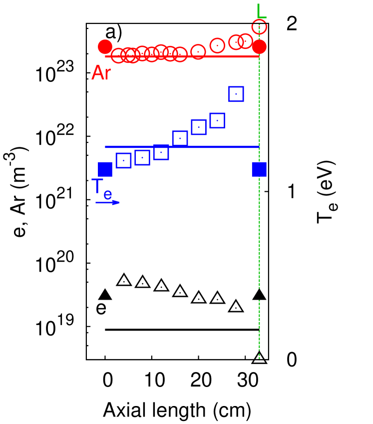
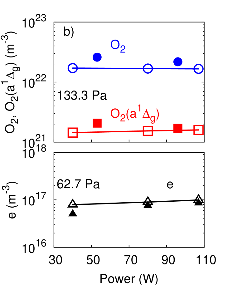
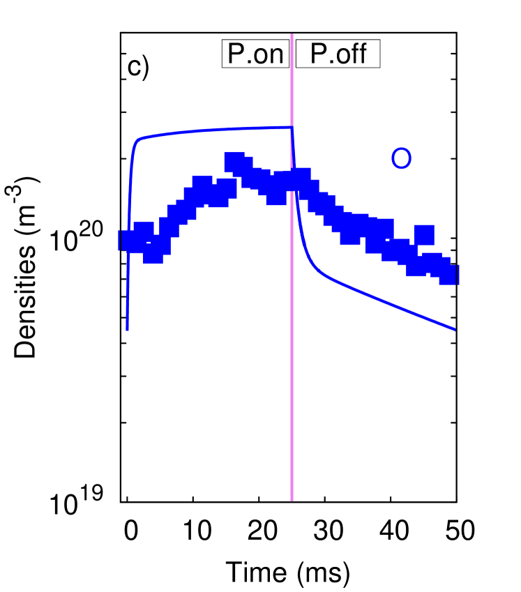
Figure 1: The measurements performed on distinct surface-wave discharges of cylindrical structures I [39] , II [40] and III [41] of table 1 and the simulation results (line or line-points). The simulation results are volume-averaged and they are comparable to the spatially-averaged measurements. a) Axially-resolved e ($\triangle$) and Ar ($\circ$) densities as well as the electron temperature T_e ($\square$) in an argon surfatron (I) together with their axial averages - denoted by $\blacktriangle$, $\bullet$ and $\blacksquare$, respectively. b) Axial-averages of e ($\blacktriangle$), O₂ ($\bullet$) and O${}_{2}(\text{a}^{1}\Delta_{\text{g}})$ ($\blacksquare$) density measurements in an oxygen surfatron (II). c) Transient O density measurements in a microwave source of SLAN type with a pulse-modulated power input (III).

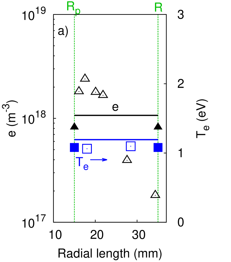
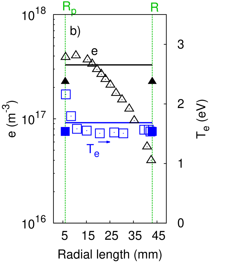
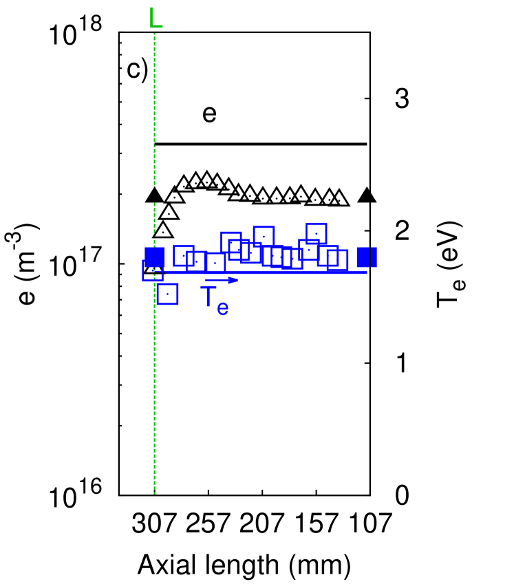
Figure 2: The measurements performed on distinct coaxial structures of IV [11] and V - see table 1 - and the simulation results (line) for a feeding gas of argon. The simulation results are volume-averaged and they are comparable to the spatially-averaged measurements. a) Radially-resolved electron density ($\triangle$) and temperature ($\square$) measurements on the discharge setup IV. The radial averages of the electron density and temperature measurements are denoted by $\blacktriangle$ and $\blacksquare$, respectively. b) Radially-resolved electron density ($\triangle$) and temperature ($\square$) measurements as well as their radial averages (denoted by $\blacktriangle$ and $\blacksquare$, respectively) on the setup V. c) Axially-resolved electron density ($\triangle$) and temperature ($\square$) measurements as well as their axial averages (denoted by $\blacktriangle$ and $\blacksquare$, respectively) on the setup V.

The simulation results and the measurements of the coaxial structures IV and V - see table 1 - for a feeding gas of argon are shown in figure 2. The radially-resolved and radially-averaged electron density and temperature are shown in figure 2-a) for a stationary plasmaline IV [11]. The same type of data is shown in figure 2-b) in the plasmaline of interest V at $30\>$Pa for an input power of $300\>$W with the gas temperature of $500\>$K and the gas flow rate of $100\>$sccm, whereas axially-resolved and axially-averaged versions are shown in figure 2-c). We observe that the radial variation is much more amplified than the axial variation and the spatially-resolved measurements are in the same order of magnitude with their spatial-averages. The simulation results show a good agreement with the stationary radially- and axially-averaged measurements.

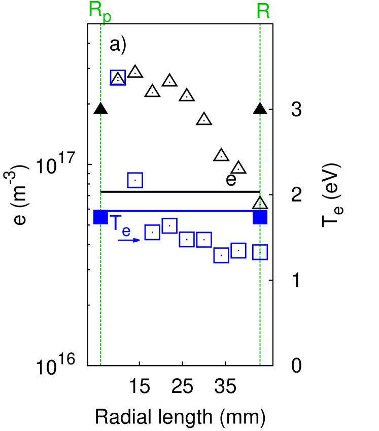
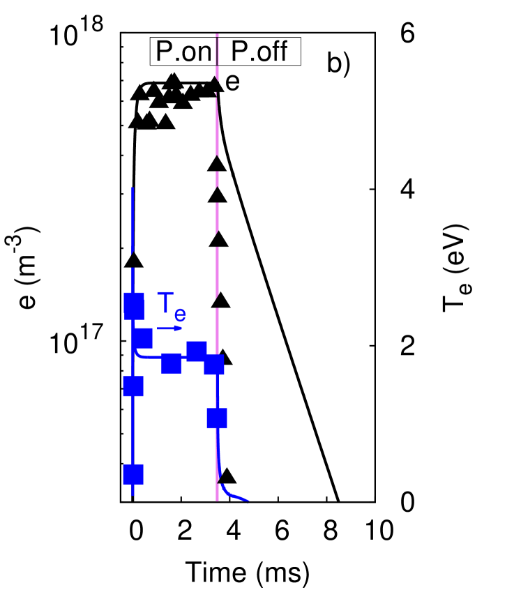
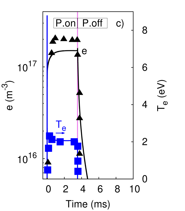
Figure 3: The measurements of the discharge setup V - see table 1 - and the simulation results (lines). The simulation results are volume-averaged and they are comparable to the spatially-averaged measurements. a) Radially-resolved electron density ($\triangle$) and temperature ($\square$) measurements as well as their radial averages (denoted by $\blacktriangle$ and $\blacksquare$, respectively) on the stationary oxygen plasma. b) Time-resolved radially-averaged electron density ($\blacktriangle$) and temperature ($\blacksquare$) measurements for a pulse-modulated power input in argon. c) Time-resolved radially-averaged measurements of electron density ($\blacktriangle$) and temperature ($\blacksquare$) for a pulse-modulated power input in oxygen.

The measurements on the discharge setup V of either argon or oxygen for continuous and pulse-modulated powers are shown in figure 3 together with the simulation results. The radially-resolved and radially-averaged electron density and temperature in continuous power oxygen plasma are given in 3-a). The power input is $600\>$W at a pressure of $25\>$Pa and the gas temperature is $500\>$K with a gas flow rate of $200\>$sccm. The transient electron density and temperature of the pulse-modulated discharge in argon and oxygen are shown in figures 3-b) and 3-c), respectively. The pressure is $30\>$Pa for argon and $25\>$Pa for oxygen discharge both at a gas temperature of $900\>$K and the peak power input for both pulse-modulated measurements is $1500\>$W. The gas flow rates are $100\>$sccm in argon and $200\>$sccm in oxygen. The simulation results agree well with the radially-averaged stationary as well as transient measurements, however, the electron decay in the argon afterglow suggests considerably smaller decay rate compared to the experimental observation. The estimation of the afterglow edge-to-centre ratio to the unity - for example, after the electrons thermally equilibrate with the background gas - imposes much faster decay rate. However, such an assumption is not preferred due to the lack of data in the afterglow spatial structures, regarding validity requirements as well as the resultant sudden change in the decay rate. We also observe that the electron temperature decays much slowly as its value decreases mostly due to the insufficient loss mechanism.

Table 2 shows the percentage of the wall loss in the net loss rate of certain species within the considered discharges. The wall flux often forms a significant portion of the net loss in both cylindrical and coaxial structures. For the dominant ions, it reaches up to $98\>\%$ for Ar⁺ and up to $58\>\%$ for O${}_{2}^{+}$. Among the neutrals, the wall flux also considerably contributes to the net loss for O, $\text{O}_{2}(a^{1}\Delta_{g})$ and $\text{O}_{2}(b^{1}\sum_{g}^{+})$, although, the maximum percentages are lower compared to those of the ions. The wall loss rates of Ar(4s) and Ar(4p) are negligible, and hence, the simulations are not sensitive to the wall de-excitation probabilities of the excited argon species.

Although the O wall recombination is an important loss mechanism, the recombination probability has only a weak effect on the simulations for a range of $0.009-1$. Because of this and due to lack of data, a recombination probability identical to that of the quartz wall is assumed at the entire radial boundaries of the coaxial structure V. Such a weak effect of the recombination probability is in contrast with the observations at low pressure oxygen plasma [30] that we also confirm with the same chemical kinetics of the current study [17]. The wall recombination is incomparably the most dominant mechanism both in the loss of oxygen atom and the production of the molecular oxygen at low pressure. However, in the relatively higher pressure regime considered, ozone-based reactions also have a significant contribution to the oxygen atom loss and to the molecular oxygen production. These reactions substantially suppress the critical role of the wall recombination probability on the surface wave discharges.

Argon species	(I)	(IV)	(V)	Oxygen species	(II)	(V)
$\text{Ar}^{+}$	$48$	$32$	$98$	$\text{O}_{2}^{+}$	$08$	$58$
Ar(4sr)	$4\times 10^{-3}$	$3\times 10^{-3}$	$3\times 10^{-2}$	O	$10$	$38$
Ar(4p)	$4\times 10^{-4}$	$4\times 10^{-5}$	$4\times 10^{-4}$	$\text{O}_{2}(a^{1}\Delta_{g})$	$25$	$29$
				$\text{O}_{2}(b^{1}\sum_{g}^{+})$	$07$	$56$

Table 2: The percentage of the wall loss rate - either equations 25 for the cylindrical or equations 26 for the coaxial structures - in the net loss rate of dominant ions and certain neutrals. Here, we only consider the discharges operated with continuous power input and refer to table 1 for the corresponding operation parameters. We show the calculation results of setup II at a power input of $107\>$W and at a pressure of $133\>$Pa.

We observe that the considered oxygen discharges are attachment dominated with $\tau_{an}K_{a}\geq 20$, hence the negative ions are not in Boltzmann equilibrium. On the other hand, the simulation results are not sensitive to the resultant variation in the Bohm velocity. The negative ion loss mechanism is dominated by the detachment as expected in the considered pressure regime [38]. A hypothetical inclusion of an axial ion edge-to-centre ratio, for example, with the critical edge electron density of the surface-wave propagation [55], are negligible on the results.

The analytically estimated radial Bessel profile is also proposed earlier in cylindrical argon [12] and oxygen discharges of opposite asymptotic $P$ limits [33, 35, 34]. The former should be disturbed due to molecular-assisted recombination in the considered case of operation conditions. A Bessel radial distribution in coaxial argon discharge is also observed [11], however, the profile transforms to a similar Gaussian-like shape as the molecular-assisted recombination dominates over the diffusion loss. The simulation results suggest that the molecular-assisted recombination dominates in setup IV, whereas the diffusive wall loss dominates in setup V. The measurements of coaxial argon and oxygen discharges suggest a profile peak closer to the inner wall compared to the analytical estimation since the power density is localized near the inner wall.

The ion edge-to-centre ratio is numerically comparable with the low-collisionality analogue ($h^{+}_{iR}=3.90\times 10^{-3}$ and $\bar{h}^{+}_{iR}=3.88\times 10^{-3}$) in argon surfatron (I) and the positive ions are volume loss dominated with a comparable wall loss rate. The value of the neutral edge-to-centre ratio is also similar with the earlier derivation for the excited argon species ($h^{N}_{iR}=1.73\times 10^{-3}$ and $\bar{h}^{N}_{iR}=2.50\times 10^{-3}$). The difference in the numerical values is due to the factor of $(2/2.405)^{2}$ and the addition of the axial walls are negligible on the numerical difference. The interchange of the ion and the neutral edge-to-centre ratios with the earlier analogues are negligible on the simulation results.

The numerical values of the ion edge-to-centre ratios significantly differ in the case of oxygen surfatron (II) due to the single electronegative region flat-topped term $\bar{h}^{+}_{iR,c}$. The ratio $\bar{h}^{+}_{iR}$ is higher than $h^{+}_{iR}$ mostly by a factor of about $10$ for a volume loss dominated positive ions within a range of degree of the electronegativity $2-5$. The interchange of the ratio with $\bar{h}^{+}_{iR}$ in the simulations reduces a variety of particle densities and raises the electron temperature. This also changes the dominant positive ion loss mechanism to the diffusive wall losses and increases the degree of electronegativity to the range $4-7$. The numerical density values are still in the same order and the usage of any edge-to-centre ratios do not lead better agreement with the considered measurements. Compared with the earlier assumption of about $0.05$ in the edge-to-volume-averaged formalism [14], the derived edge-to-centre ratio is smaller by a factor of about $0.17$. A factor of difference between the edge-to-centre and edge-to-volume-averaged formalisms is about $0.5$. The neutral edge-to-centre ratios $h^{N}_{iR}$ and $\bar{h}^{N}_{iR}$ are similar in their numerical values and their interchange with each other is not effective on the simulation results. The difference between the ion edge-to-centre ratios is even larger in setup III. The ratio $\bar{h}^{+}_{iR}$ is larger than $h^{+}_{iR}$ with a factor of about $200$ for $\alpha\approx 12$. However, the positive ions are volume loss dominated and the interchange of the edge-to-centre ratios do not significantly alter the simulation results.

V Conclusions

A volume-averaged global model is developed for the surface-wave discharges of cylindrical and coaxial structures for both the electropositive and the electronegative plasmas. A set of edge-to-centre density ratios for the neutrals and the positive ions are derived based on an analytical one-dimensional model in order to estimate regarding wall loss rates. The analytical model of charged species is based on the three-component plasma with an assumption of constant or piecewise constant degree of electronegativity as suggested by a variety of earlier studies [7, 36, 23] in the considered collisionality regime. The simulation results are compared with various volume-averaged measurements, and a good agreement is obtained in argon or oxygen surface-wave discharges of cylindrical and coaxial structures for both continuous and pulse-modulated power input. The calculations show that the wall flux is often an important loss mechanism. A numerical comparison is made between the derived edge-to-centre ratios in the cylindrical structure and their analogues that are used in the low-pressure plasmas. A difference is observed only in the electronegative oxygen plasma, where the validity of the low-pressure analogue is expired [36, 37, 38].

The inhomogeneity in the discharge is often significantly localized, for example, inside the surfatron launcher, near the dielectric surface. However, a homogeneity assumption with a zeroth order degree of homogeneity still holds in the volume-averaged quantities within the numerical range of the model sensitivity. Analytically estimated profiles are in approximate agreement with the earlier studies with a maximum located more radially outward in the coaxial structure compared to measurements. The resultant edge-to-centre ratios sufficiently describe the wall flux rates for an experimentally confirmed volume-averaged particle densities within the sensitivity of the model. The power transfer efficiency of the coaxial discharge of interest (V) is only estimated ignoring the small portion of the axial length with a smaller outer radius. A more accurate estimation can be acquired by a coupling of the microwave propagation with an appropriate spatially-resolved plasma model. The chemical sets are adopted from earlier studies in literature and a throughout analysis of the reaction mechanisms is still required for further accuracy.

Appendix A Derivation of ion edge-to-centre ratios

The general solution of the ions is earlier given in the form

$$n^{+}_{i}(r)=C_{1}J_{0}\left(\chi r/R\right)+C_{2}Y_{0}\left(\chi r/R\right),$$ (31)

where the boundary conditions and the normalization of the maximum to the unity define the special - dimensionless - form. At any Bohm point $r^{\prime}_{B}$ that is in the vicinity of the corresponding radial plasma wall $R^{\prime}$, the ions satisfy

$$-D_{i+}\frac{\partial n^{+}_{i}}{\partial r}\left.\right|_{r^{\prime}_{B}}=(\pm)u_{+,BE}n^{+}_{i}\left.\right|_{r^{\prime}_{B}},$$ (32)

where ${r^{\prime}_{B}}$ corresponds to either the single radial Bohm point of the cylindrical ($R^{\prime}=R$) or double radial Bohm points of the coaxial structure ($R^{\prime}=R$ and $R^{\prime}=R_{p}$) and only the inner wall ($R^{\prime}=R_{p}$) incorporates the negative sign (-) on the right-hand side. The edge-to-centre ratio at any radial wall is [19]

$$h^{+}_{iR^{\prime}}=\frac{1}{1+\alpha}(u_{BE}/u_{B})n^{+}_{i}\left.\right|_{r^{\prime}_{B}},$$ (33)

where the centre value - corresponds to the maximum value for the coaxial structure - is unity via normalisation, $\frac{1}{1+\alpha}$ is an additional factor of normalization in the electronegative discharges [30] and $(u_{BE}/u_{B})$ is the effect of the electronegativity on the Bohm velocity. Assuming negligibly small sheath length , $\left|r^{\prime}_{B}-R^{\prime}\right|/R\gg 1$, the Taylor series expansion at $R^{\prime}$ leads

$$\frac{\partial n^{+}_{i}}{\partial r}\left.\right|_{r^{\prime}_{B}}\approx\frac{\partial n^{+}_{i}}{\partial r}\left.\right|_{R^{\prime}}.$$ (34)

Hence, using this with equation 32, $n^{+}_{i}\left.\right|_{r^{\prime}_{B}}$ can be approximated by the following relation

$$n^{+}_{i}\left.\right|_{r^{\prime}_{B}}\approx(\mp)\frac{\chi D_{+}}{Ru_{+,BE}}(C_{1}J_{1}\left(\chi R^{\prime}/R\right)+C_{2}Y_{1}\left(\chi R^{\prime}/R\right)).$$ (35)

However, it is observed that the edge-to-centre ratios via this approximation often cause computationally unstable simulations. A numerically equivalent and computationally more stable alternative can be estimated from this approximation in the following form

$$n^{+}_{i}\left.\right|_{r^{\prime}_{B}}\approx\left(1+\left(\frac{Ru_{+,BE}}{\chi D_{+}\left(C_{1}J_{1}\left(\chi R^{\prime}/R\right)+C_{2}Y_{1}\left(\chi R^{\prime}/R\right)\right)}\right)^{2}\right)^{-1/2}.$$ (36)

For the sake of computational stability, we prefer the latter form with the edge-to-centre ratio

$$h^{+}_{iR^{\prime}}\approx\frac{1}{1+\alpha}(u_{BE}/u_{B})\left(1+\left(\frac{Ru_{+,BE}}{\chi D_{i+}\left(C_{1}J_{1}\left(\chi R^{\prime}/R\right)+C_{2}Y_{1}\left(\chi R^{\prime}/R\right)\right)}\right)^{2}\right)^{-1/2}.$$ (37)

Appendix B Chemical kinetics

Chemical sets by Gudmundsson et al [50] are adopted in argon plasma simulations as well as argon excimer reactions and three body recombination by Jimenez et al [12] and Kabouzi et al [51]. A previously adopted species and reaction sets are used in the oxygen simulations without a reduction [14].

Figure 4: Energy level diagram of Ar and $\text{O}_{2}$ plasma species.

Table 3: Argon plasma reactions. We adopt the chemical set by Gudmundsson et al [50] and additionally include the argon excimer ion kinetics as well as three-body recombination by Jimenez et al [12] or Kabouzi et al [51]. The units of the rate coefficients are $\text{m}^{3}\text{s}^{-1}$ and those of electron and gas temperatures are eV and K, respectively, if not stated otherwise.

#	Reaction	Rate Coefficient	Ref
1	$e+\text{Ar}\rightarrow\text{Ar}^{+}+2e$	$2.3\times 10^{-14}T_{e}^{0.59}e^{-17.44/T_{e}}$	[56]
2	$e+\text{Ar}\rightarrow e+\text{Ar}(4s_{m})$	$5.0\times 10^{-15}e^{-12.64/T_{e}}$	[57]
3	$e+\text{Ar}\rightarrow e+\text{Ar}(4s_{m})$	$1.4\times 10^{-15}e^{-12.42/T_{e}}$	[57]
4	$e+\text{Ar}\rightarrow e+\text{Ar}(4s_{r})$	$1.9\times 10^{-15}e^{-12.60/T_{e}}$	[57]
5	$e+\text{Ar}\rightarrow e+\text{Ar}(4s_{r})$	$2.7\times 10^{-16}e^{-12.14/T_{e}}$	[57]
6	$e+\text{Ar}\rightarrow e+\text{Ar}(4p)$	$2.1\times 10^{-14}e^{-13.13/T_{e}}$	[58]
7	$e+\text{Ar}(4s_{m})\rightarrow e+\text{Ar}$	$4.3\times 10^{-16}T_{e}^{0.74}$	[59]
8	$e+\text{Ar}(4s_{m})\rightarrow\text{Ar}^{+}+2e$	$6.8\times 10^{-15}T_{e}^{0.67}e^{-4.20/T_{e}}$	[60]
9	$e+\text{Ar}(4s_{m})\rightarrow e+\text{Ar}(4s_{r})$	$3.7\times 10^{-13}$	[61]
10	$e+\text{Ar}(4s_{m})\rightarrow e+\text{Ar}(4p)$	$8.9\times 10^{-13}T_{e}^{0.51}e^{-1.59/T_{e}}$	[60]
11	$2\text{Ar}(4s_{m})\rightarrow 2\text{Ar}$	$2.0\times 10^{-13}$
12?	$\text{Ar}+\text{Ar}^{+}\rightarrow\text{Ar}+\text{Ar}^{+}$	$2.2\times 10^{-16}$	[62]
13	$\text{Ar}(4s_{m})+\text{Ar}(4s_{r})\rightarrow\text{Ar}+\text{Ar}^{+}+e$	$2.1\times 10^{-15}$	[63]
14	$\text{Ar}(4p)+\text{Ar}(4p)\rightarrow\text{Ar}+\text{Ar}^{+}+e$	$5.0\times 10^{-16}$	[60]
14	$\text{Ar}(4s_{m})+\text{Ar}(4s_{m})\rightarrow\text{Ar}+\text{Ar}^{+}+e$	$6.4\times 10^{-16}$	[61]
15	$e+\text{Ar}(4p)\rightarrow\text{Ar}^{+}+2e$	$1.8\times 10^{-13}T_{e}^{0.61}e^{-2.61/T_{e}}$	[60]
16	$e+\text{Ar}(4p)\rightarrow\text{Ar}(4s_{r})+e$	$3.0\times 10^{-13}T_{e}^{0.51}$	[59]
17	$e+\text{Ar}(4p)\rightarrow\text{Ar}(4s_{m})+e$	$3.0\times 10^{-13}T_{e}^{0.51}$	[59]
18	$e+\text{Ar}(4p)\rightarrow\text{Ar}+e$	$3.9\times 10^{-16}T_{e}^{0.71}$	[59]
19	$\text{Ar}+\text{Ar}(4s_{m})\rightarrow 2\text{Ar}$	$2.1\times 10^{-21}$	[63]
20	$e+\text{Ar}(4s_{r})\rightarrow\text{Ar}+e$	$4.3\times 10^{-16}T_{e}^{0.74}$	[59]
21	$e+\text{Ar}(4s_{r})\rightarrow\text{Ar}(4s_{m})+e$	$9.1\times 10^{-13}$	[61]
22	$e+\text{Ar}(4s_{r})\rightarrow\text{Ar}(4p)+e$	$8.9\times 10^{-13}T_{e}^{0.51}e^{-1.59/T_{e}}$	[60]
23	$\text{Ar}(4s_{r})\rightarrow\text{Ar}$	$1.0\times 10^{05}\>1/$s	[64]
24	$\text{Ar}(4p)\rightarrow\text{Ar}$	$3.2\times 10^{07}\>1/$s	[59]
25	$\text{Ar}(4p)\rightarrow\text{Ar}(4s_{m})$	$3.0\times 10^{07}\>1/$s	[65]
26	$\text{Ar}(4p)\rightarrow\text{Ar}(4s_{r})$	$3.0\times 10^{07}\>1/$s	[65]
27	$\text{Ar}_{2}^{+}+e\rightarrow\text{Ar}(4s_{m})+\text{Ar}$	$1.04\times 10^{-12}(T_{e}[K]/300)^{-0.67}(1-e^{-418/T_{h}})/(1-0.31e^{-418/T_{h}})$	[51]
28	$\text{Ar}_{2}^{+}+e\rightarrow\text{Ar}(4s_{r})+\text{Ar}$	$1.04\times 10^{-12}(T_{e}[K]/300)^{-0.67}(1-e^{-418/T_{h}})/(1-0.31e^{-418/T_{h}})$	[51]
29	$\text{Ar}_{2}^{+}+e\rightarrow\text{Ar}^{+}+\text{Ar}+e$	$1.11\times 10^{-12}e^{-(2.94-3(T_{h}[eV]-0.026))/T_{e}}$	[51]
30	$\text{Ar}^{+}+2\text{Ar}\rightarrow\text{Ar}_{2}^{+}+\text{Ar}$	$2.25\times 10^{-43}(T_{h}/300)^{-0.4}$	[51]
31	$\text{Ar}_{2}^{+}+\text{Ar}\rightarrow\text{Ar}^{+}+2\text{Ar}$	$5.22\times 10^{-16}(T_{h}[eV])^{-1.0}e^{-1.304/T_{h}[eV]}$	[51]
32	$\text{Ar}^{+}+2e\rightarrow\text{Ar}(4p)+e$	$5.00\times 10^{-39}(T_{e})^{-4.5}$	[66]
33	$\text{Ar}^{+}+2e\rightarrow\text{Ar}+e$	$8.75\times 10^{-39}T_{e}^{-2.25}$	[67]

Table 4: Electron - Oxygen reactions [14]. The rate coefficients are given in $\text{m}^{3}\text{s}^{-1}$ and the electron temperature is given in eV. The symbol “*” is used to specify the inverse reaction coefficients calculated by detailed balancing.

#	Reaction	Rate Coefficient	Ref
1	$e+\text{O}_{2}\rightarrow\text{O}_{2}^{+}+2e$	$2.01\times 10^{-15}T_{e}^{1.09}e^{-12.41/T_{e}}$	[68]
2	$e+\text{O}_{2}\rightarrow\text{O}(^{3}P)+\text{O}^{+}+2e$	$1.04\times 10^{-14}T_{e}^{1.11}e^{-21.27/T_{e}}$	[68]
3	$e+\text{O}_{2}\rightarrow\text{O}(^{3}P)+\text{O}^{-}$	$1.12\times 10^{-15}T_{e}^{-1.41}e^{-6.16/T_{e}}$	[69]
4	$e+\text{O}_{2}(a^{1}\Delta_{g})\rightarrow\text{O}(^{3}P)+\text{O}^{-}$	$4.33\times 10^{-15}T_{e}^{-1.39}e^{-5.17/T_{e}}$	[69]
5	$e+\text{O}_{2}(a^{1}\Delta_{g})\rightarrow\text{O}(^{1}D)+\text{O}^{-}$	$1.01\times 10^{-15}T_{e}^{-1.46}e^{-7.36/T_{e}}$	[69]
6	$e+\text{O}_{2}(A^{3}\sum_{u}^{+},...)\rightarrow\text{O}(^{3}P)+\text{O}^{-}$	$5.77\times 10^{-16}T_{e}^{-0.90}e^{-0.12/T_{e}}$	[70]
7	$e+\text{O}(^{3}P)\rightarrow\text{O}^{+}+2e$	$4.75\times 10^{-15}T_{e}^{0.78}e^{-14.27/T_{e}}$	[71]
8	$e+\text{O}^{-}\rightarrow\text{O}(^{3}P)+2e$	$4.64\times 10^{-14}T_{e}^{0.50}e^{-3.44/T_{e}}$	[72]
9	$e+\text{O}_{2}\rightarrow\text{O}(^{3}P)+\text{O}(^{1}D)+e$	$8.45\times 10^{-15}T_{e}^{0.38}e^{-11.84/T_{e}}$	[73]
10	$e+\text{O}_{2}\rightarrow\text{O}(^{3}P)+\text{O}(^{3}P)+e$	$9.49\times 10^{-16}T_{e}^{0.38}e^{-11.84/T_{e}}$	[73]
11	$e+\text{O}_{2}\rightarrow\text{O}(^{1}D)+\text{O}(^{1}D)+e$	$9.49\times 10^{-17}T_{e}^{0.38}e^{-11.84/T_{e}}$	[73]
12	$e+\text{O}_{2}\rightarrow\text{O}^{+}+\text{O}^{-}+e$	$4.12\times 10^{-14}T_{e}^{-0.25}e^{-20.80/T_{e}}$	[74]
13	$e+\text{O}(^{3}P)\rightarrow\text{O}(^{1}D)+e$	$2.19\times 10^{-14}T_{e}^{-0.57}e^{-4.10/T_{e}}$	[75]	*
14	$e+\text{O}_{2}\rightarrow\text{O}_{2}(a^{1}\Delta_{g})+e$	$1.25\times 10^{-14}T_{e}^{-0.97}e^{-5.51/T_{e}}$	[76]	*
15	$e+\text{O}_{2}\rightarrow\text{O}_{2}(b^{1}\sum_{g}^{+})+e$	$3.84\times 10^{-15}T_{e}^{-1.05}e^{-5.71/T_{e}}$	[76]	*
16	$e+\text{O}_{2}\rightarrow\text{O}_{2}(A^{3}\sum_{u}^{+},...)+e$	$2.39\times 10^{-14}T_{e}^{-1.00}e^{-9.52/T_{e}}$	[77]	*
17	$e+\text{O}_{2}(a^{1}\Delta_{g})\rightarrow\text{O}_{2}(b^{1}\sum_{g}^{+})+e$	$6.69\times 10^{-15}T_{e}^{-0.56}e^{-1.73/T_{e}}$	[78]	*
18	$e+\text{O}_{2}(a^{1}\Delta_{g})\rightarrow\text{O}_{2}(A^{3}\sum_{u}^{+},...)+e$	$7.23\times 10^{-14}T_{e}^{-1.25}e^{-7.63/T_{e}}$	[78]	*
19	$e+\text{O}_{2}(b^{1}\sum_{g}^{+})\rightarrow\text{O}_{2}(A^{3}\sum_{u}^{+},...)+e$	$8.47\times 10^{-14}T_{e}^{-1.23}e^{-7.12/T_{e}}$	[78]	*
20	$e+\text{O}_{3}\rightarrow\text{O}_{2}+\text{O}^{-}$	$3.24\times 10^{-15}T_{e}^{-0.94}e^{-0.91/T_{e}}$	[79]
21	$e+\text{O}_{3}\rightarrow\text{O}(^{3}P)+\text{O}_{2}^{-}$	$9.56\times 10^{-16}T_{e}^{-1.26}e^{-0.95/T_{e}}$	[79]
22	$e+\text{O}_{3}\rightarrow\text{O}_{2}+\text{O}(^{3}P)+e$	$1.42\times 10^{-14}T_{e}^{-0.68}e^{-2.60/T_{e}}$	[80]
23	$e+\text{O}_{3}\rightarrow\text{O}_{2}(a^{1}\Delta_{g})+\text{O}(^{3}P)+e$	$4.16\times 10^{-15}T_{e}^{-0.73}e^{-3.15/T_{e}}$	[80]
24	$e+\text{O}_{3}\rightarrow\text{O}_{2}(a^{1}\Delta_{g})+\text{O}(^{1}D)+e$	$6.68\times 10^{-15}T_{e}^{-0.82}e^{-4.07/T_{e}}$	[80]
25	$e+\text{O}_{3}\rightarrow\text{O}_{2}(b^{1}\sum_{g}^{+})+\text{O}(^{1}D)+e$	$1.34\times 10^{-13}T_{e}^{-0.87}e^{-6.63/T_{e}}$	[80]
26	$e+\text{O}_{2}^{-}\rightarrow\text{O}_{2}+2e$	$5.74\times 10^{-14}T_{e}^{0.58}e^{-4.68/T_{e}}$	[81]
27	$e+\text{O}_{3}^{-}\rightarrow\text{O}_{3}+2e$	$3.43\times 10^{-14}T_{e}^{0.22}e^{-8.81/T_{e}}$	[82]
28	$e+\text{O}_{3}^{-}\rightarrow\text{O}_{2}+\text{O}(^{3}P)+2e$	$2.69\times 10^{-14}T_{e}^{0.06}e^{-20.10/T_{e}}$	[82]
29	$e+\text{O}_{3}^{-}\rightarrow\text{O}_{2}+\text{O}^{-}+e$	$3.67\times 10^{-14}e^{-8.26/T_{e}}$	[82]
30	$e+\text{O}_{2}^{+}\rightarrow\text{O}(^{3}P)+\text{O}(^{1}D)$	$2.20\times 10^{-14}T_{e}^{-0.50}$	[83]

Table 5: Oxygen-Oxygen reactions [14]. The rate coefficients and the gas temperature are given in $\text{m}^{3}\text{s}^{-1}$ and K, respectively.

#	Reaction	Rate Coefficient	Ref
31	$\text{O}_{2}^{+}+\text{O}^{-}\rightarrow\text{O}_{2}+\text{O}(^{3}P)$	$2.60\times 10^{-14}(300/T_{h})^{0.44}$	[83]
32	$\text{O}^{+}+\text{O}^{-}\rightarrow 2\text{O}(^{3}P)$	$4.00\times 10^{-14}(300/T_{h})^{0.43}$	[83]
33	$\text{O}(^{3}P)+\text{O}^{-}\rightarrow\text{O}_{2}+e$	$2.30\times 10^{-16}$	[84]
34	$\text{O}_{2}+\text{O}^{+}\rightarrow\text{O}(^{3}P)+\text{O}_{2}^{+}$	$2.10\times 10^{-17}(300/T_{h})^{0.50}$	[85]
35	$\text{O}_{2}+\text{O}(^{1}D)\rightarrow\text{O}_{2}+\text{O}(^{3}P)$	$2.56\times 10^{-17}e^{67/T_{h}}$	[85]
36	$\text{O}(^{3}P)+\text{O}(^{1}D)\rightarrow 2\text{O}(^{3}P)$	$8.00\times 10^{-18}$	[85]
37	$\text{O}_{2}(a^{1}\Delta_{g})+\text{O}^{-}\rightarrow\text{O}(^{3}P)+\text{O}_{2}^{-}$	$4.75\times 10^{-17}$	[84]
38	$\text{O}_{2}^{+}+\text{O}_{2}^{-}\rightarrow 2\text{O}_{2}$	$2.01\times 10^{-13}(300/T_{h})^{0.50}$	[85]
39	$\text{O}^{+}+\text{O}_{2}^{-}\rightarrow\text{O}_{2}+\text{O}(^{3}P)$	$2.70\times 10^{-13}(300/T_{h})^{0.50}$	[86]
40	$\text{O}(^{3}P)+\text{O}_{2}^{-}\rightarrow\text{O}_{2}+\text{O}^{-}$	$3.31\times 10^{-16}$	[85]
41	$\text{O}_{2}(a^{1}\Delta_{g})+\text{O}_{2}^{-}\rightarrow 2\text{O}_{2}+e$	$2.00\times 10^{-16}$	[87]
42	$\text{O}_{2}+\text{O}^{-}\rightarrow\text{O}_{3}+e$	$5.00\times 10^{-21}$	[86]
43	$\text{O}_{2}(a^{1}\Delta_{g})+\text{O}^{-}\rightarrow\text{O}_{3}+e$	$1.42\times 10^{-16}$	[84]
44	$\text{O}_{3}+\text{O}^{+}\rightarrow\text{O}_{2}+\text{O}_{2}^{+}$	$1.00\times 10^{-16}$	[86]
45	$\text{O}(^{3}P)+\text{O}_{3}\rightarrow 2\text{O}_{2}$	$1.81\times 10^{-17}e^{-2300/T_{h}}$	[85]
46	$\text{O}_{3}+\text{O}^{-}\rightarrow\text{O}(^{3}P)+\text{O}_{3}^{-}$	$5.30\times 10^{-16}$	[85]
47	$\text{O}(^{3}P)+\text{O}_{3}^{-}\rightarrow\text{O}_{2}+\text{O}_{2}^{-}$	$1.00\times 10^{-16}$	[85]
48	$\text{O}(^{3}P)+\text{O}_{3}^{-}\rightarrow 2\text{O}_{2}+e$	$3.00\times 10^{-16}$	[85]
49	$\text{O}_{2}^{+}+\text{O}_{3}^{-}\rightarrow\text{O}_{2}+\text{O}_{3}$	$2.00\times 10^{-13}(300/T_{h})^{0.50}$	[85]
50	$\text{O}_{2}^{+}+\text{O}_{3}^{-}\rightarrow 2\text{O}(^{3}P)+\text{O}_{3}$	$1.01\times 10^{-13}(300/T_{h})^{0.50}$	[85]
51	$\text{O}_{3}+\text{O}_{2}^{-}\rightarrow\text{O}_{2}+\text{O}_{3}^{-}$	$4.00\times 10^{-16}$	[85]
52	$\text{O}(^{3}P)+\text{O}_{2}^{-}\rightarrow\text{O}_{3}+e$	$3.30\times 10^{-16}$	[88]
53	$\text{O}_{2}+\text{O}(^{1}D)\rightarrow\text{O}_{2}(a^{1}\Delta_{g})+\text{O}(^{3}P)$	$1.00\times 10^{-18}$	[85]
54	$\text{O}_{2}(b^{1}\sum_{g}^{+})+\text{O}^{-}\rightarrow\text{O}_{2}+\text{O}(^{3}P)+e$	$6.90\times 10^{-16}$	[89]
55	$\text{O}_{2}(b^{1}\sum_{g}^{+})+\text{O}(^{3}P)\rightarrow\text{O}_{2}(a^{1}\Delta_{g})+\text{O}(^{3}P)$	$8.10\times 10^{-20}$	[90]
56	$\text{O}_{2}+\text{O}_{2}(b^{1}\sum_{g}^{+})\rightarrow\text{O}_{2}+\text{O}_{2}(a^{1}\Delta_{g})$	$3.79\times 10^{-22}(300/T_{h})^{-2.40}e^{-281/T_{h}}$	[90]
57	$\text{O}_{2}(a^{1}\Delta_{g})+\text{O}(^{3}P)\rightarrow\text{O}_{2}+\text{O}(^{3}P)$	$1.30\times 10^{-22}$	[91]
58	$\text{O}_{2}^{+}+\text{O}^{-}\rightarrow 3\text{O}(^{3}P)$	$2.60\times 10^{-14}(300/T_{h})^{0.44}$	[83]
59	$\text{O}_{2}+\text{O}_{2}(a^{1}\Delta_{g})\rightarrow 2\text{O}_{2}$	$2.20\times 10^{-24}(300/T_{h})^{-0.80}$	[86]
60	$\text{O}_{2}(A^{3}\sum_{u}^{+},...)+\text{O}(^{3}P)\rightarrow\text{O}_{2}(b^{1}\sum_{g}^{+})+\text{O}(^{1}D)$	$1.35\times 10^{-18}$	[92]
61	$\text{O}_{2}+\text{O}_{3}\rightarrow 2\text{O}_{2}+\text{O}(^{3}P)$	$7.26\times 10^{-16}e^{-11400/T_{h}}$	[85]
62	$\text{O}_{2}(a^{1}\Delta_{g})+\text{O}_{2}(a^{1}\Delta_{g})\rightarrow\text{O}_{2}+\text{O}_{2}(b^{1}\sum_{g}^{+})$	$1.80\times 10^{-24}(300/T_{h})^{-3.80}e^{700/T_{h}}$	[93]
63	$\text{O}_{2}(a^{1}\Delta_{g})+\text{O}_{2}(a^{1}\Delta_{g})\rightarrow 2\text{O}_{2}$	$5.50\times 10^{-29}(300/T_{h})^{-0.50}$	[94]
64	$\text{O}_{2}(b^{1}\sum_{g}^{+})+\text{O}_{3}\rightarrow 2\text{O}_{2}+\text{O}(^{3}P)$	$1.50\times 10^{-17}$	[95]
65	$\text{O}_{2}(a^{1}\Delta_{g})+\text{O}_{3}\rightarrow 2\text{O}_{2}+\text{O}(^{3}P)$	$6.01\times 10^{-17}e^{-2853/T_{h}}$	[95]
66	$\text{O}_{2}+\text{O}_{2}(A^{3}\sum_{u}^{+},...)\rightarrow 2\text{O}_{2}(b^{1}\sum_{g}^{+})$	$2.90\times 10^{-19}$	[96]
67	$\text{O}_{2}^{+}+\text{O}_{2}^{-}\rightarrow\text{O}_{2}+2\text{O}(^{3}P)$	$1.01\times 10^{-13}(300/T_{h})^{0.50}$	[85]
68	$\text{O}_{2}(A^{3}\sum_{u}^{+},...)\rightarrow\text{O}_{2}+\hbar\nu$	$6.251/s$	[97]
69	$\text{O}_{2}(A^{3}\sum_{u}^{+},...)+\text{O}(^{3}P)\rightarrow\text{O}_{2}+\text{O}(^{3}P)$	$4.95\times 10^{-18}$	[92]
70	$\text{O}_{2}(A^{3}\sum_{u}^{+},...)+\text{O}(^{3}P)\rightarrow\text{O}_{2}(a^{1}\Delta_{g})+\text{O}(^{1}D)$	$2.70\times 10^{-18}$	[92]
71	$2\text{O}_{2}(b^{1}\sum_{g}^{+})\rightarrow\text{O}_{2}+\text{O}_{2}(a^{1}\Delta_{g})$	$3.60\times 10^{-23}(300/T_{h})^{-0.50}$	[98]

Table 6: Three body reactions [14]. The rate coefficients and the gas temperature are given in $\text{m}^{6}\text{s}^{-1}$ and K, respectively, whereas the electron temperature is in eV.

#	Reaction	Rate Coefficient	Ref
72	$e+e+\text{O}^{+}\rightarrow\text{O}(^{3}P)+e$	$7.89\times 10^{-39}T_{e}^{-4.50}$	[85]
73	$e+\text{O}_{2}+\text{O}_{2}\rightarrow\text{O}_{2}+\text{O}_{2}^{-}$	$2.26\times 10^{-42}T_{e}^{0.50}$	[99]
74	$\text{O}+\text{O}_{2}+\text{O}_{2}\rightarrow\text{O}_{3}+\text{O}_{2}$	$6.3\times 10^{-46}(300/T_{h})^{2}$	[100]
75	$\text{O}_{2}+\text{O}(^{3}P)+\text{O}(^{3}P)\rightarrow\text{O}(^{3}P)+\text{O}_{3}$	$2.15\times 10^{-40}e^{345/T_{h}}$	[25]
76	$e+\text{O}_{2}+\text{O}(^{3}P)\rightarrow\text{O}(^{3}P)+\text{O}_{2}^{-}$	$1.00\times 10^{-43}$	[85]
77	$e+\text{O}_{2}+\text{O}(^{3}P)\rightarrow\text{O}_{2}+\text{O}^{-}$	$1.00\times 10^{-43}$	[85]
78	$e+\text{O}_{2}+\text{O}^{+}\rightarrow\text{O}_{2}+\text{O}(^{3}P)$	$1.00\times 10^{-38}$	[85]
79	$\text{O}_{2}+\text{O}_{2}+\text{O}^{-}\rightarrow\text{O}_{2}+\text{O}_{3}^{-}$	$1.00\times 10^{-42}(300/T_{h})$	[85]
80	$\text{O}_{2}+\text{O}^{+}+\text{O}^{-}\rightarrow\text{O}_{2}+\text{O}_{2}$	$2.10\times 10^{-37}(300/T_{h})^{2.50}$	[85]
81	$\text{O}_{2}+\text{O}_{2}^{+}+\text{O}^{-}\rightarrow\text{O}_{2}+\text{O}_{3}$	$2.01\times 10^{-37}(300/T_{h})^{2.50}$	[85]
82	$\text{O}_{2}+\text{O}_{2}+\text{O}(^{3}P)\rightarrow\text{O}_{2}+\text{O}_{3}$	$6.90\times 10^{-46}(300/T_{h})^{1.25}$	[85]
83	$\text{O}_{2}+\text{O}(^{3}P)+\text{O}(^{3}P)\rightarrow\text{O}_{2}+\text{O}_{2}(A^{3}\sum_{u}^{+},...)$	$1.20\times 10^{-46}$	[96]
84	$\text{O}_{2}+\text{O}_{2}(a^{1}\Delta_{g})+\text{O}(^{3}P)\rightarrow\text{O}_{2}+\text{O}_{2}+\text{O}(^{3}P)$	$1.00\times 10^{-44}$	[92]
85	$3\text{O}(^{3}P)\rightarrow\text{O}_{2}(a^{1}\Delta_{g})+\text{O}(^{3}P)$	$1.93\times 10^{-47}(300/T_{h})^{0.63}$	[90]
86	$\text{O}_{2}+\text{O}(^{3}P)+\text{O}(^{3}P)\rightarrow\text{O}_{2}+\text{O}_{2}(a^{1}\Delta_{g})$	$6.93\times 10^{-47}(300/T_{h})^{0.63}$	[90]

Table 7: Elastic electronic collisions included in the simulations.

#	Collision	Ref
1	$e+\text{Ar}$	[101]
2	$e+\text{O}_{2}$	[102]
3	$e+\text{O}$	[103]
4	$e+\text{O}_{3}$	[80]

Table 8: Chemical reactions induced at the wall.

#	Reaction	probability($\gamma$) $R_{p}$	probability($\gamma$) $R$	Ref
1	$\text{Ar}(4s,4p)+\text{wall}\rightarrow\text{Ar}$	$1$	$1$	[12]
1	$\text{O}(^{3}P,^{1}D)+\text{wall}\rightarrow 1/2\text{O}_{2}$	$0.09$	$0.09$	[104]
2	$\text{O}(^{1}D)+\text{wall}\rightarrow\text{O}(^{3}P)$	$0.1$	$0.1$	[25]
3	$\text{O}_{2}(a^{1}\Delta_{g})+\text{wall}\rightarrow\text{O}_{2}$	$0.007$	$0.007$	[105]
4	$\text{O}_{2}(b^{1}\sum_{g}^{+})+\text{wall}\rightarrow\text{O}_{2}$	$0.1$	$0.1$	[25]
5	$\text{O}_{2}(A^{3}\sum_{u}^{+},...)+\text{wall}\rightarrow\text{O}_{2}$	$0.1$	$0.1$	[25]

References

- [1] S. Steves, B. Ozkaya, C.-N. Liu, O. Ozcan, N. Bibinov, G. Grundmeier, and P. Awakowicz. Silicon oxide barrier films deposited on PET foils in pulsed plasmas: influence of substrate bias on deposition process and film properties. Journal of Physics D: Applied Physics, 46(8):084013, 2013.
- [2] H. Bahre, K. Bahroun, H. Behm, S. Steves, P. Awakowicz, M. Böke, Ch. Hopmann, and J. Winter. Surface pre-treatment for barrier coatings on polyethylene terephthalate. Journal of Physics D: Applied Physics, 46(8):084012, 2013.
- [3] A. S. C. Nave, F. Mitschker, P. Awakowicz, and J. Röpcke. Spectroscopic studies of microwave plasmas containing hexamethyldisiloxane. Journal of Physics D: Applied Physics, 49(39):395206, 2016.
- [4] V. M. M. Glaude, M. Moisan, R. Pantel, P. Leprince, and J. Marec. Axial electron density and wave power distributions along a plasma column sustained by the propagation of a surface microwave. Journal of Applied Physics, 51(11):5693–5698, 1980.
- [5] Ts. Petrova, E. Benova, G. Petrov, and I. Zhelyazkov. Self-consistent axial modeling of surface-wave-produced discharges at low and intermediate pressures. Phys. Rev. E, 60:875–886, Jul 1999.
- [6] K. Makasheva and A. Shivarova. Surface-wave-produced plasmas in a diffusion-controlled regime. Physics of Plasmas, 8(3):836–845, 2001.
- [7] C. M. Ferreira. Modelling of a low-pressure plasma column sustained by a surface wave. Journal of Physics D: Applied Physics, 16(9):1673, 1983.
- [8] C.M. Ferreira, L.L. Alves, M. Pinheiro, and A.B. Sa. Modeling of low-pressure microwave discharges in Ar, He, and O2: similarity laws for the maintenance field and mean power transfer. Plasma Science, IEEE Transactions on, 19(2):229–239, Apr 1991.
- [9] K. Kutasi, V. Guerra, and P. Sa. Theoretical insight into Ar-O2 surface-wave microwave discharges. Journal of Physics D: Applied Physics, 43(17):175201, 2010.
- [10] L. L. Alves, S. Letout, and C. Boisse-Laporte. Modeling of surface-wave discharges with cylindrical symmetry. Phys. Rev. E, 79:016403, Jan 2009.
- [11] S. Rahimi, M. Jimenez-Diaz, S. Hübner, E. H. Kemaneci, J. J. A. M. van der Mullen, and J. van Dijk. A two-dimensional modelling study of a coaxial plasma waveguide. Journal of Physics D: Applied Physics, 47(12):125204, 2014.
- [12] M. Jimenez-Diaz, E. A. D. Carbone, J. van Dijk, and J. J. A. M. van der Mullen. A two-dimensional Plasimo multiphysics model for the plasma-electromagnetic interaction in surface wave discharges: the surfatron source. J. Phys. D: Appl. Phys., 45:335204, 2012.
- [13] A. Obrusník and Z. Bonaventura. Studying a low-pressure microwave coaxial discharge in hydrogen using a mixed 2d/3d fluid model. Journal of Physics D: Applied Physics, 48(6):065201, 2015.
- [14] E. Kemaneci, E. Carbone, M. Jimenez-Diaz, W. Graef, S. Rahimi, J. van Dijk, and G. Kroesen. Modelling of an intermediate pressure microwave oxygen discharge reactor: from stationary two-dimensional to time-dependent global (volume-averaged) plasma models. Journal of Physics D: Applied Physics, 48(43):435203, 2015.
- [15] P. Chabert and N. Braithwaite. Physics of Radio-Frequency Plasmas. Cambridge: Cambridge University Press, 2011.
- [16] E. H. Kemaneci. Modelling of Plasmas with Complex Chemistry: Application to Microwave Deposition Reactors. PhD thesis, TUE, 2014.
- [17] E. Kemaneci, J.-P. Booth, P. Chabert, J. van Dijk, T. Mussenbrock, and R. P. Brinkmann. A computational analysis of the vibrational levels of molecular oxygen in low-pressure stationary and transient radio-frequency oxygen plasma. Plasma Sources Science and Technology, 25(2):025025, 2016.
- [18] V. A. Godyak. Soviet Radio Frequency Discharge Research. Delphic, Falls Church, VA, 1986.
- [19] M. A. Lieberman and A. J. Lichtenberg. Principles of Plasma Discharges and Materials Processing. New Jersey: John Wiley Sons, 2005.
- [20] A. J. Lichtenberg, V. Vahedi, and M. A. Lieberman. Modeling of electronegative plasma discharges. J. Appl. Phys., 75(75):2339, 1994.
- [21] A. J. Lichtenberg, I. G. Kouznetsov, Y. T. Lee, M. A. Lieberman, I. D. Kaganovich, and L. D. Tsendin. Modelling plasma discharges at high electronegativity. Plasma Sources Science and Technology, 6(3):437, 1997.
- [22] A. J. Lichtenberg, M. A. Lieberman, I. G. Kouznetsov, and T. H. Chung. Transitions and scaling laws for electronegative discharge models. Plasma Sources Science and Technology, 9(1):45, 2000.
- [23] S. Kim, M. A. Lieberman, A. J. Lichtenberg, and J. T. Gudmundsson. Improved volume-averaged model for steady and pulsed-power electronegative discharges. Journal of Vacuum Science & Technology A, 24(6):2025–2040, 2006.
- [24] D. D. Monahan and M. M. Turner. Global models of electronegative discharges: Critical evaluation and practical recommendations. Plasma Sources Sci. Technol., 17:045003, 2008.
- [25] E. G. Thorsteinsson and J. T. Gudmundsson. The low pressure ClO2 discharge and the role of ClO. Plasma Sources Science and Technology, 19(5):055008, 2010.
- [26] D. A. Toneli, R. S. Pessoa, M. Roberto, and J. T. Gudmundsson. On the formation and annihilation of the singlet molecular metastables in an oxygen discharge. Journal of Physics D: Applied Physics, 48(32):325202, 2015.
- [27] T. Lafleur and P. Chabert. Edge-to-center density ratios in low-temperature plasmas. Plasma Sources Science and Technology, 24(2):025017, 2015.
- [28] J.-L. Raimbault and P. Chabert. Edge-to-center plasma density ratio in high density plasma sources. Plasma Sources Science and Technology, 18(1):014017, 2009.
- [29] P. Chabert. An expression for the hl factor in low-pressure electronegative plasma discharges. Plasma Sources Science and Technology, 25(2):025010, 2016.
- [30] C. Lee and M. A. Lieberman. Global model of Ar, O2, Cl2, and Ar/O2 high-density plasma discharges. Journal of Vacuum Science & Technology A, 13(2):368–380, 1995.
- [31] P. J. Chantry. A simple formula for diffusion calculations involving wall reflection and low density. J. Appl. Phys., 62:1141, 1987.
- [32] E. Stoffels, W. W. Stoffels, D. Vender, M. Kando, G. M. W. Kroesen, and F. J. de Hoog. Negative ions in a radio-frequency oxygen plasma. Phys. Rev. E, 51:2425–2435, Mar 1995.
- [33] C. M. Ferreira, G. Gousset, and M. Touzeau. Quasi-neutral theory of positive columns in electronegative gases. Journal of Physics D: Applied Physics, 21(9):1403, 1988.
- [34] P. G. Daniels and R. N. Franklin. The positive column in electronegative gases-a boundary layer approach. Journal of Physics D: Applied Physics, 22(6):780, 1989.
- [35] P. G. Daniels, R. N. Franklin, and J. Snell. The contracted positive column in electronegative gases. Journal of Physics D: Applied Physics, 23(7):823, 1990.
- [36] R. N. Franklin and J. Snell. Modelling discharges in electronegative gases. Journal of Physics D: Applied Physics, 32(17):2190, 1999.
- [37] R. N. Franklin. A critique of models of electronegative plasmas. Plasma Sources Science and Technology, 10(2):162, 2001.
- [38] R N Franklin. Electronegative plasmas - why are they so different? Plasma Sources Science and Technology, 11(3A):A31, 2002.
- [39] S. Hübner, E. Iordanova, J. M. Palomares, E. A. D. Carbone, and J. J. A. M. van der Mullen. Rayleigh scattering on a microwave surfatron plasma to obtain axial profiles of the atom density and temperature. Eur. Phys. J. Appl. Phys., 58(2):20802, 2012.
- [40] A. Granier, S. Pasquiers, C. Boisse-Laporte, R. Darchicourt, P. Leprince, and J. Marec. Characterisation of a low-pressure oxygen discharge created by surface waves. Journal of Physics D: Applied Physics, 22(10):1487, 1989.
- [41] A. Georg, J. Engemann, and A. Brockhaus. Investigation of a pulsed oxygen microwave plasma by time-resolved two-photon allowed laser-induced fluorescence. Journal of Physics D: Applied Physics, 35(9):875, 2002.
- [42] J. A. Bittencourt. Fundamentals of plasma physics. Springer, 2004.
- [43] J.-L. Raimbault, L. Liard, J.-M. Rax, P. Chabert, A. Fruchtman, and G. Makrinich. Steady-state isothermal bounded plasma with neutral dynamics. Physics of Plasmas, 14(1), 2007.
- [44] A. V. Phelps. The diffusion of charged particles in collisional plasmas: free and ambipolar diffusion at low and moderate pressures. J. Res. Natl. Inst. Stand. Technol., 95(4):407, 1990.
- [45] A. Hartgers. Modelling of a fluorescent lamp plasma. PhD thesis, Eindhoven University of Technology, The Netherlands, 2003.
- [46] E. A. Bogdanov and A. A. Kudryavtsev. The conditions for realization of the Boltzmann distribution of negative ions in a plasma. Technical Physics Letters, 27(11):905, 2001.
- [47] I. G. Kouznetsov, A. J. Lichtenberg, and M. A. Lieberman. Modelling electronegative discharges at low pressure. Plasma Sources Science and Technology, 5(4):662, 1996.
- [48] J. B. Thompson. Negative ions in the positive column of the oxygen discharge. Proceedings of the Physical Society, 73(5):818, 1959.
- [49] N. St. J. Braithwaite and J. E. Allen. Boundaries and probes in electronegative plasmas. Journal of Physics D: Applied Physics, 21(12):1733, 1988.
- [50] J. T. Gudmundsson and E. G. Thorsteinsson. Oxygen discharges diluted with argon: dissociation processes. Plasma Sources Sci. Technol, 16:399, 2007.
- [51] Y. Kabouzi, D. B. Graves, E. Castanos-Martinez, and M. Moisan. Modeling of atmospheric-pressure plasma columns sustained by surface waves. Phys. Rev. E, 75:016402, Jan 2007.
- [52] E. Kemaneci, E. Carbone, J.-P. Booth, W. Graef, J. van Dijk, and G. Kroesen. Global (volume-averaged) model of inductively coupled chlorine plasma: Influence of Cl wall recombination and external heating on continuous and pulse-modulated plasmas. Plasma Sources Science and Technology, 23(4):045002, 2014.
- [53] E. G. Thorsteinsson and J. T. Gudmundsson. A global (volume averaged) model of a chlorine discharge. Plasma Sources Sci. Technol., 19:015001, 2010.
- [54] S. Hübner. Poly-diagnostic study of low pressure microwave plasmas. PhD thesis, Eindhoven University of Technology, The Netherlands, 2013.
- [55] J. L. Jauberteau and I. Jauberteau. Dielectric properties in microwave remote plasma sustained in argon: Expanding plasma conditions. Physics of Plasmas, 19(11), 2012.
- [56] H. C. Straub, P. Renault, B. G. Lindsay, K. A. Smith, and R. F. Stebbings. Absolute partial and total cross sections for electron-impact ionization of argon from threshold to 1000 ev. Phys. Rev. A, 52:1115–1124, Aug 1995.
- [57] K. Tachibana. Excitation of the 1,1, 1, and 1 levels of argon by low-energy electrons. Phys. Rev. A, 34:1007–1015, Aug 1986.
- [58] E. Eggarter. Comprehensive optical and collision data for radiation action. ii. ar. The Journal of Chemical Physics, 62(3):833–847, 1975.
- [59] S. Ashida, C. Lee, and M. A. Lieberman. Spatially averaged (global) model of time modulated high density argon plasmas. J. Vac. Sci. Technol. A, 13:2498, 1995.
- [60] F. Kannari, M. Obara, and T. Fujioka. An advanced kinetic model of electron-beam-excited KrF lasers including the vibrational relaxation in KrF*(B) and collisional mixing of KrF*(B,C). Journal of Applied Physics, 57(9):4309–4322, 1985.
- [61] C. M. Ferreira, J. Loureiro, and A. Ricard. Populations in the metastable and the resonance levels of argon and stepwise ionization effects in a low-pressure argon positive column. Journal of Applied Physics, 57(1):82–90, 1985.
- [62] R. H. Neynaber, S. M. Trujillo, and E. W. Rothe. Symmetric-resonance charge transfer in Ar from 0.1-20 eV using merging beams. Phys. Rev., 157:101–102, May 1967.
- [63] N. L. Bassett and D. J. Economou. Effect of Cl2 additions to an argon glow discharge. Journal of Applied Physics, 75(4):1931–1939, 1994.
- [64] G. S. Hurst, E. B. Wagner, and M. G. Payne. Energy transfer from the resonance states Ar(1P1) and Ar(3P1) to ethylene. The Journal of Chemical Physics, 61(9):3680–3685, 1974.
- [65] M.-H. Lee, S.-H. Jang, and C.-W. Chung. On the multistep ionizations in an argon inductively coupled plasma. Physics of Plasmas, 13(5), 2006.
- [66] A. N. Bhoj and M. J. Kushner. Avalanche process in an idealized lamp: II. modelling of breakdown in Ar/Xe electric discharges. Journal of Physics D: Applied Physics, 37(18):2510, 2004.
- [67] Yu.P. Raizer. Gas Discharge Physics. Springer, 1991.
- [68] H. C. Straub, P. Renault, B. G. Lindsay, K. A. Smith, and R. F. Stebbings. Absolute partial cross sections for electron-impact ionization of H2, N2, and O2 from threshold to 1000 eV. Phys. Rev. A, 54:2146–2153, 1996.
- [69] T. Jaffke, M. Meinke, R. Hashemi, L. G. Christophorou, and E. Illenberger. Dissociative electron attachment to singlet oxygen. Chem. Phys. Lett., 193:62–68, 1992.
- [70] D. Hayashi and K. Kadota. Efficient production of O by dissociative attachment of slow electrons to highly excited metastable oxygen molecules. Japan. J. Appl. Phys., 38(part 1):225, 1999.
- [71] Y.-K. Kim and J.-P. Desclaux. Ionization of carbon, nitrogen, and oxygen by electron impact. Phys. Rev. A, 66:012708, 2002.
- [72] H. Deutsch, P. Scheier, K. Becker, and T. D. Märk. Calculated cross-sections for the electron-impact detachment from negative ions using the Deutsch-Märk (DM) formalism. Chem. Phys. Lett., 382:26–31, 2003.
- [73] P. C. Cosby. Electron-impact dissociation of oxygen. J. Chem. Phys., 98:9560, 1993.
- [74] D. Rapp and D. D. Briglia. Total cross sections for ionization and attachment in gases by electron impact. II. Negative-ion formation. J. Chem. Phys., 43:1480, 1965.
- [75] J. P. Doering. Absolute differential and integral electron excitation cross sections for atomic oxygen, 9. Improved cross section for the 3P 1D transition from 4.0 to 30 eV. J. Geophys. Res., 97:19531, 1992.
- [76] T. W. Shyn and C. J. Sweeney. Differential electronic-excitation cross sections of molecular oxygen by electron impact: The a and states. Phys. Rev. A, 47:1006–1008, 1993.
- [77] T. W. Shyn and C. J. Sweeney. Measurement of absolute differential excitation cross sections of molecular oxygen by electron impact: Decomposition of the Herzberg pseudocontinuum. Phys. Rev. A, 62:022711, 2000.
- [78] M. Tashiro, K. Morokuma, and J. Tennyson. R-matrix calculation of electron collisions with electronically excited O2 molecules. Phys. Rev. A, 73:052707, 2006.
- [79] S. A. Rangwala, S. V. K. Kumar, E. Krishnakumar, and N. J. Mason. Cross sections for the dissociative electron attachment to ozone. J. Phys. B: At. Mol. Opt. Phys., 32:3795, 1999.
- [80] M. Gupta and K. L. Baluja. Electron collisions with an ozone molecule using the R-matrix method. J. Phys. B: At. Mol. Opt. Phys., 38:4057, 2005.
- [81] H. Deutsch, K. Becker, M. Probst, W. Zhu, and T. D. Märk. Calculated absolute cross-sections for the electron-induced detachment of the B, O, BO-, and CN- anions using the Deutsch-Märk (DM) formalism. Int. J. Mass Spectrom., 277:151–154, 2008.
- [82] K. Seiersen, J. Bak, H. Bluhme, M. J. Jensen, S. B. Nielsen, and L. H. Andersen. Electron-impact detachment of O, NO and SO ions. Phys. Chem. Chem. Phys., 5:4814–4820, 2003.
- [83] J. T. Gudmundsson and M. A. Lieberman. Recombination rate coefficients in oxygen discharges. Technical Report RH-16-2004, Science Institute, University of Iceland, 2004.
- [84] S. G. Belostotsky, D. J. Economou, D. V. Lopaev, and T. V. Rakhimova. Negative ion destruction by O(3P) atoms and O molecules in an oxygen plasma. Plasma Sources Sci. Technol., 14:532, 2005.
- [85] B. Eliasson and U. Kogelshatz. Basic data for modeling of electrical discharges in gases: Oxygen report. Technical Report KLR-11C, Brown Boveri Konzernforschung, CH5405, Baden, 1986.
- [86] I. A. Kossyi, A. Yu Kostinsky, A. A. Matveyev, and V. P. Silakov. Kinetic scheme of the non-equilibrium discharge in nitrogen-oxygen mixtures. Plasma Sources Sci. Technol., 1:207, 1992.
- [87] F. C. Fehsenfeld, D. L. Albritton, J. A. Burt, and H. I. Schiff. Associative-detachment reactions of O-and O by O2(). Canadian Journal of Chemistry, 47(10):1793–1795, 1969.
- [88] F. C. Fehsenfeld, A. L. Schmeltekopf, H. I. Schiff, and E. E. Ferguson. Laboratory measurements of negative ion reactions of atmospheric interest. Planetary and Space Science, 15(2):373 – 379, 1967.
- [89] N. L. Aleksandrov. Sov. Phys.—Tech. Phys., 23:806, 1978.
- [90] B. F. Gordiets anf C. M. Ferreira, V. L. Guerra, J. M. A. H. Loureiro, J. Nahorny, D. Pagnon, M. Touzeau, and M. Vialle. Kinetic model of a low-pressure N2-O2 flowing glow discharge. IEEE Trans. Plasma Sci., 23:750–768, 1995.
- [91] I. D. Clark and R. P. Wayne. The reaction of O2(a) with atomic nitrogen and with atomic oxygen. Chemical Physics Letters, 3(6):405 – 407, 1969.
- [92] A. N. Vasiljeva, K. S. Klopovskiy, A. S. Kovalev, D. V. Lopaev, Y. A. Mankelevich, N. A. Popov, A. T. Rakhimov, and T. V. Rakhimova. On the possibility of O2() production by a non-self-sustained discharge for oxygen–iodine laser pumping. J. Phys. D: Appl. Phys., 37(17):2455, 2004.
- [93] N. Cohen and K. R. Westberg. Chemical kinetic data sheets for hightemperature chemical reactions. J. Phys. Chem. Ref. Data, 12(3):531, 1983.
- [94] P. Borrell and N. H. Rich. The rate constant for the “dimol” transition of singlet oxygen, O2(a), and the likely symmetry of the emitting species. Chem. Phys. Lett., 99(2):144, 1983.
- [95] J. Y. Jeong, J. Park, I. Henins, S. E. Babayan, V. J. Tu, G. S. Selwyn, G. Ding, and R. F. Hicks. Reaction chemistry in the afterglow of an oxygen-helium, atmospheric-pressure plasma. J. Phys. Chem., 104(34):8027, 2000.
- [96] R. D. Kenner and E. A. Ogryzlo. Deactivation of O2(A) by O2, O, and Ar. Int. J. Chem. Kinet., 12(7):501, 1980.
- [97] R. D. Kenner and E. A. Ogryzlo. Rate constant for the deactivation of O2(A) by N2. Chem. Phys. Lett., 103(3):209, 1983.
- [98] D. S. Stafford and M. J. Kushner. O2 production in He/O2 mixtures in flowing low pressure plasmas. J. Appl. Phys., 96(5):2451, 2004.
- [99] H. Shimamori and R. W. Fessenden. Thermal electron attachment to oxygen and van der waals molecules containing oxygen. J. Chem. Phys., 74(1):453, 1981.
- [100] D. V. Lopaev, E. M. Malykhin, and S. M. Zyryanov. Surface recombination of oxygen atoms in O2 plasma at increased pressure: II. Vibrational temperature and surface production of ozone. Journal of Physics D: Applied Physics, 44(1):015202, 2011.
- [101] J. T. Gudmundsson. Notes on the electron excitation rate coefficients for argon and oxygen discharges. Technical Report RH-21-2002, Science Institute, University of Iceland, Reykjavik, Iceland, 2002.
- [102] Y. Itikawa. Cross sections for electron collisions with oxygen molecules. Journal of Physical and Chemical Reference Data, 38(1):1–20, 2009.
- [103] Y. Itikawa and A. Ichimura. Cross sections for collisions of electrons and photons with atomic oxygen. Journal of Physical and Chemical Reference Data, 19(3):637–651, 1990.
- [104] L. Stafford, J. Guha, and V. M. Donnely. Recombination probability of oxygen atoms on dynamic stainless steel surfaces in inductively coupled O2 plasmas. J. Vac. Sci. Technol. A, 26:455, 2008.
- [105] R. L. Sharpless and T. G. Slanger. Surface chemistry of metastable oxygen. II destruction of O2(). J. Chem. Phys., 91:7947, 1989.