CMB-lensing beyond the leading order: temperature and polarization anisotropies

Abstract

We investigate the weak lensing corrections to the CMB temperature and polarization anisotropies. We consider all the effects beyond the leading order: post-Born corrections, LSS corrections and, for the polarization anisotropies, the correction due to the rotation of the polarization direction between the emission at the source and the detection at the observer. We show that the full next-to-leading order correction to the B-mode polarization is not negligible on small scales and is dominated by the contribution from the rotation, this is a new effect not taken in account in previous works. Considering vanishing primordial gravitational waves, the B-mode correction due to rotation is comparable to cosmic variance for $\ell\gtrsim 3500$, in contrast to all other spectra where the corrections are always below that threshold for a single multipole. Moreover, the sum of all the effects is larger than cosmic variance at high multipoles, showing that higher-order lensing corrections to B-mode polarization are in principle detectable.

1 Introduction

The temperature and polarization anisotropies of the cosmic microwave background (CMB) are the most precious cosmological datasets. It is fair to say that virtually all high precision cosmological measurements involve the CMB. The reason for this is twofold: on the one hand there is excellent data available Ade:2014afa ; Naess:2014wtr ; Crites:2014prc ; Story:2014hni ; Adam:2015rua ; Planck:2015xua ; Ade:2015zua ; Keisler:2015hfa and on the other hand CMB fluctuations are theoretically well understood and can be calculated perturbatively. The CMB success story is by no means over, we expect more precision data to arrive especially for polarization and reconstruction of the cosmic lens map Abazajian:2016yjj ; DiValentino:2016foa .

As it is well known, CMB fluctuations are lensed by foreground large scale structure (LSS) and this effect is rather large (up to 10% and more) on small scales Seljak:1995ve ; Lewis:2006fu ; RuthBook . Therefore the question is justified whether higher order contributions to lensing might be relevant. We naively expect them to be of the order of the square of the first order contribution, hence 1% and therefore it is necessary to include them as numerical CMB calculations Lewis:1999bs ; Lesgourgues:2011re ; Blas:2011rf ; Lesgourgues:2013bra aim at a precision of 0.1%. On the other hand, present CMB codes do take into account some of the non-linearities by summing up a series of ’ladder diagrams’ into an exponential Lewis:2006fu ; RuthBook . It is easy to check that including these non-linearities is requested to achieve the precision goal.

The question which we address in this paper is: what about the other non-linearities which are not included in this sum? Might they also be relevant? These are mainly contributions coming from the fact that the deflection angle of the photons at higher order can no longer be computed assuming the photons move along their unperturbed path, but the perturbation of the photon path has to be taken into account. These are the so-called ‘post-Born corrections’. We have already studied this problem for the temperature anisotropies in a previous paper Marozzi:2016uob . The present paper is a follow up on that work. We complete the previous study by calculating also the effects on polarization. Furthermore, here we treat also the non-linearities of the matter distribution perturbatively. This is more consistent than just using a Halofit model Smith:2002dz ; Takahashi:2012em , as it allows us to correctly take into account the higher order statistics (3- and 4-point functions) assuming Gaussian first order perturbations. We neglect the radial displacement corrections induced by the time delay effect (which indeed is not a lensing contribution). As shown in Hu:2001yq , these corrections are at most of the order $\mathcal{O}\left(10^{-4}\right)$, apart for the temperature-E-mode cross correlation power spectrum for which can reach the order of $\mathcal{O}\left(10^{-3}\right)$. We do, however, take into account all effects of second and third order lensing. This includes also the induced vector and tensor modes. These modes are especially important for B-polarisation as they effectively rotate the photon polarisation.

In addition to our work, there have been three other publications on this topic Hagstotz:2014qea ; Pratten:2016dsm ; Lewis:2016tuj . In the first paper, an important cancellation which reduces the final result by more than an order of magnitude has been missed. In Pratten:2016dsm our so called ’third group’ terms, which vanish when assuming Gaussian statistics and are very relevant for the final result, are not included. In the most recent publication Lewis:2016tuj these terms are included, but the rotation of the polarization which is induced by second order lensing is not considered. We discuss it here for the first time and we actually find that it is the dominant correction for $B$-polarization.

In this paper we present the methodology of our calculations and numerical results for the corrections of CMB temperature and polarization anisotropies by next-to-leading order lensing. In an accompanying letter Marozzi:2016und we discuss the relevance of our findings for future CMB experiments.

The paper is organized as follows. In the next section we summarize the small deflection angle approximation for CMB lensing beyond linear order, and present the expressions for the deflection angle up to third order. In Sect. 3 we translate the results into harmonic space, ’$\boldsymbol{\ell}$ space’. We also compare the expressions for temperature anisotropies with the corresponding terms for the polarization spectra at all orders in perturbation theory. In Sect. 4 we briefly recollect the results for the post-Born corrections to the lensed power spectrum of the CMB temperature anisotropies first given in Marozzi:2016uob considering also the non-Gaussian nature of the deflection angle at higher order. In Sect. 5 we evaluate the contributions from higher orders in the gravitational potential (or equivalently in the matter density) to corrections of the lensed power spectrum of the CMB temperature and polarization anisotropies. Following Pratten:2016dsm ; Lewis:2016tuj we call them ‘LSS corrections’. In Sect. 6 we derive the last missing contribution coming from the fact that parallel transported polarization direction changes along the path of the photon from the source to the observer. This contribution which turns out to be very substantial has been missed in previous work. Our results are summarized in Sect. 7, where we evaluate the different contributions numerically considering a Halofit matter power spectrum. In Sect. 8 we conclude. Several technical aspects and calculations are presented in four appendices.

2 Weak lensing corrections beyond leading order in real space

We want to determine the effect of lensing on the CMB temperature and polarization anisotropies beyond the well studied leading order from first order perturbation theory Lewis:2006fu ; RuthBook .

Following the derivation of the post-Born correction to temperature anisotropies in Marozzi:2016uob , we first generalize the results of Lewis:2006fu ; RuthBook writing the following relation between the lensed and unlensed temperature anisotropies $\mathcal{M}$ and polarization tensor $\mathcal{P}_{mn}$ of the photon field valid up to fourth order in the deflection angles $\theta^{a(i)}$ (the superscript $(i)$ denotes the order).

$$\tilde{\mathcal{M}}(x^{a}) \equiv \mathcal{M}\left(x^{a}+\delta\theta^{a}\right)\simeq\mathcal{M}(x^{a})+\sum_{i=1}^{4}\theta^{b(i)}\nabla_{b}\mathcal{M}(x^{a})$$ (2.1)

$$+ \frac{1}{2}\sum_{i+j\leq 4}\theta^{b(i)}\theta^{c(j)}\nabla_{b}\nabla_{c}\mathcal{M}(x^{a})$$

$$+ \frac{1}{6}\sum_{i+j+k\leq 4}\theta^{b(i)}\theta^{c(j)}\theta^{d(k)}\nabla_{b}\nabla_{c}\nabla_{d}\mathcal{M}(x^{a})$$

$$+ \frac{1}{24}\theta^{b(1)}\theta^{c(1)}\theta^{d(1)}\theta^{e(1)}\nabla_{b}\nabla_{c}\nabla_{d}\nabla_{e}\mathcal{M}(x^{a})\,,$$

$$\tilde{\mathcal{P}}_{mn}(x^{a}) \equiv \mathcal{P}_{mn}\left(x^{a}+\delta\theta^{a}\right)$$

$$\simeq \mathcal{P}_{mn}(x^{a})+\sum_{i=1}^{4}\theta^{b(i)}\nabla_{b}\mathcal{P}_{mn}(x^{a})$$

$$+ \frac{1}{2}\sum_{i+j\leq 4}\theta^{b(i)}\theta^{c(j)}\nabla_{b}\nabla_{c}\mathcal{P}_{mn}(x^{a})$$

$$+ \frac{1}{6}\sum_{i+j+k\leq 4}\theta^{b(i)}\theta^{c(j)}\theta^{d(k)}\nabla_{b}\nabla_{c}\nabla_{d}\mathcal{P}_{mn}(x^{a})$$

$$+ \frac{1}{24}\theta^{b(1)}\theta^{c(1)}\theta^{d(1)}\theta^{e(1)}\nabla_{b}\nabla_{c}\nabla_{d}\nabla_{e}\mathcal{P}_{mn}(x^{a})\,.$$

A consistent treatment of the polarization in the form of $\mathcal{P}_{mn}$ or, using the Stokes parameters $\mathcal{Q}$ and $\mathcal{U}$, in the form of $\mathcal{P}=\mathcal{Q}+i\mathcal{U}$ and $\bar{\mathcal{P}}=\mathcal{Q}-i\mathcal{U}$ has to consider that the polarization tensor is parallel-transported along the perturbed photon geodesics. Neglecting this effect (we shall add it at a second stage in Sect. 6) we can substitute $\mathcal{P}_{mn}$ with $\mathcal{P}$ and $\bar{\mathcal{P}}$. An over-bar denotes complex conjugation.

Following Marozzi:2016uob , we can then write

$$\tilde{\mathcal{M}}(x^{a}) \simeq \mathcal{A}^{(0)}(x^{a})+\sum_{i=1}^{4}\mathcal{A}^{(i)}(x^{a})+\sum_{\begin{subarray}{c}i+j\leq 4\\ 1\leq i\leq j\end{subarray}}\mathcal{A}^{(ij)}(x^{a})$$ (2.3)

$$+ \sum_{\begin{subarray}{c}i+j+k\leq 4\\ 1\leq i\leq j\leq k\end{subarray}}\mathcal{A}^{(ijk)}(x^{a})+\mathcal{A}^{(1111)}(x^{a})\,,$$

$$\tilde{\mathcal{P}}(x^{a}) \simeq \mathcal{D}^{(0)}(x^{a})+\sum_{i=1}^{4}\mathcal{D}^{(i)}(x^{a})+\sum_{\begin{subarray}{c}i+j\leq 4\\ 1\leq i\leq j\end{subarray}}\mathcal{D}^{(ij)}(x^{a})$$ (2.4)

$$+ \sum_{\begin{subarray}{c}i+j+k\leq 4\\ 1\leq i\leq j\leq k\end{subarray}}\mathcal{D}^{(ijk)}(x^{a})+\mathcal{D}^{(1111)}(x^{a})\,,\$$

where

$$\mathcal{A}^{(i_{1}i_{2}....i_{n})}(x^{a})=$$

$$\!\!\!\!\!\!\!\!\!\!\!\!=\frac{{\rm Perm}(i_{1}i_{2}....i_{n})}{n!}\theta^{b(i_{1})}\theta^{c(i_{2})}.....\nabla_{b}\nabla_{c}.......\mathcal{M}(x^{a})\,,$$ (2.5)

$$\mathcal{D}^{(i_{1}i_{2}....i_{n})}(x^{a})=$$

$$\!\!\!\!\!\!\!\!\!\!\!\!=\frac{{\rm Perm}(i_{1}i_{2}....i_{n})}{n!}\theta^{b(i_{1})}\theta^{c(i_{2})}.....\nabla_{b}\nabla_{c}.......\mathcal{P}(x^{a})\,,$$ (2.6)

where $\mathcal{A}^{(0)}(x^{a})\equiv\mathcal{M}(x^{a})$, $\mathcal{D}^{(0)}(x^{a})\equiv\mathcal{P}(x^{a})$ and ${\rm Perm}(i_{1}i_{2}....i_{n})$ denotes the number of permutation of the set $(i_{1}i_{2}....i_{n})$.

We introduce also the Weyl potential

$$\Phi_{W}=\frac{1}{2}\left(\Phi+\Psi\right)\,$$ (2.7)

in terms of the Bardeen potentials $\Phi$ and $\Psi$. The lensing potential $\psi$ to the last scattering surface is then determined by

$$\psi({\bf n},z_{s}) = \frac{-2}{\eta_{o}-\eta_{s}}\int_{\eta_{s}}^{\eta_{o}}d\eta\frac{\eta-\eta_{s}}{\eta_{o}-\eta}\Phi_{W}((\eta-\eta_{o}){\bf n},\eta)$$ (2.8)

$$= -2\int_{0}^{r_{s}}dr^{\prime}\frac{r_{s}-r^{\prime}}{r_{s}r^{\prime}}\Phi_{W}(-r^{\prime}{\bf n},\eta_{o}-r^{\prime})\,,$$

where $\bf{n}$ is the direction of photon propagation, $\eta$ denotes conformal time and $r$ the comoving distance, $r=\eta_{o}-\eta$, where $\eta_{o}$ stands for present time. The index _s indicates the corresponding quantity evaluated at the last scattering surface. The first order deflection angle is simply the gradient of the lensing potential Bartelmann:1999yn ; RuthBook . Beyond the linear order, we need to account also for the lensing of the direction $\bf n$ on the path of the photon. Then one obtains the following expressions for the deflection angle up to third perturbative order Fanizza:2015swa

$$\theta^{a(1)} = -2\int_{0}^{r_{s}}\!dr^{\prime}\frac{r_{s}-r^{\prime}}{r_{s}\,r^{\prime}}\nabla^{a}\Phi_{W}(r^{\prime})\,,$$ (2.9)

$$\theta^{a(2)} = -2\int_{0}^{r_{s}}\!dr^{\prime}\frac{r_{s}-r^{\prime}}{r_{s}\,r^{\prime}}\left[\nabla^{a}\Phi_{W}^{(2)}(r^{\prime})\right.$$ (2.10)

$$\left.+\nabla_{b}\nabla^{a}\Phi_{W}(r^{\prime})\theta^{b(1)}(r^{\prime})\right]\,,$$

$$\theta^{a(3)}\! = \!-2\int_{0}^{r_{s}}\!dr^{\prime}\frac{r_{s}-r^{\prime}}{r_{s}\,r^{\prime}}\!\left[\nabla^{a}\Phi_{W}^{(3)}(r^{\prime})\right.$$ (2.11)

$$\left.+\nabla_{b}\nabla^{a}\Phi_{W}(r^{\prime})\theta^{b(2)}(r^{\prime})+\nabla_{b}\nabla^{a}\Phi_{W}^{(2)}(r^{\prime})\theta^{b(1)}(r^{\prime})\!\right.$$

$$\left.+\frac{1}{2}\nabla_{b}\nabla_{c}\nabla^{a}\Phi_{W}(r^{\prime})\theta^{b(1)}(r^{\prime})\theta^{c(1)}(r^{\prime})\right]\,.$$

Latin letters $a,b,c,d$ run over the two directions on the sphere. In Eqs. (2.9-2.11) we consider the terms with the maximal number of transverse derivatives, including the ones that come from expanding the Weyl potential, $\Phi_{W}$, to higher order. Note that $\theta^{a(2)}$ as well as $\theta^{a(3)}$ are not purely scalar perturbations, they also contain vector contributions as, for example, the curl of $\nabla_{b}\nabla^{a}\Phi_{W}\theta^{b(1)}$ does not vanish. But for our purpose a decomposition of the higher order deflection angle into scalar and vector parts are of no particular use. On the other hand, let us point out that we have neglected the second order vector and tensor perturbations of the metric appearing as a consequence of the nonlinear coupling among scalar, vector and tensor in the Einstein equation. These corrections are subleading with respect to the ones discussed here.

Let us also remind that the Taylor expansion in Eqs. (2.1) and (LABEL:IniExp) holds in the approximation of small deflection angles, i.e. when the deflection angle is much smaller than the angular separations related to a given $C_{\ell}$. This is valid for an angular separation of about $4.5$ arc minutes which corresponds to $\ell\lesssim 2500$ (see Seljak:1995ve ; RuthBook ; Lewis:2006fu ). In this work, we adopt the small deflection angle approximation for the second and third order deflection angles only, which are much smaller than this value, as a consequence our results are valid to much higher $\ell$s and we can safely present them up to $\ell=3500$.

3 Weak lensing corrections of the power spectra

We evaluate the lensing correction to the angular power spectra $C^{\mathcal{M}}_{\ell}$, $C^{\mathcal{E}\mathcal{M}}_{\ell}$, $C^{\mathcal{E}}_{\ell}$ and $C^{\mathcal{B}}_{\ell}$ in the flat sky limit. In this approximation, see e.g. RuthBook , we replace the combination $(\ell,m)$ with a 2-dimensional vector $\boldsymbol{\ell}$. Therefore, the angular position is then the 2-dimensional Fourier transform of the position in $\boldsymbol{\ell}$ space at redshift $z$. For a generic variable $Y(z,{\bf x})$ we have

$$Y(z,{\bf x})=\frac{1}{2\pi}\int d^{2}\ell\ Y(z,\boldsymbol{\ell})e^{-i\boldsymbol{\ell}\cdot{\bf x}}\,,$$ (3.1)

and

$$\langle Y(z_{1},\boldsymbol{\ell})\bar{Y}(z_{2},\boldsymbol{\ell}\,^{\prime})\rangle=\delta\left(\boldsymbol{\ell}-\boldsymbol{\ell}\,^{\prime}\right)C_{\ell}^{Y}(z_{1},z_{2})\,,$$ (3.2)

while for polarization we have ($\varphi_{\ell}$ denotes the polar angle in $\boldsymbol{\ell}$-space)

$$\mathcal{P}(z,{\bf x})=-\frac{1}{2\pi}\int d^{2}\ell\ \left[\mathcal{E}(z,\boldsymbol{\ell})+i\mathcal{B}(z,\boldsymbol{\ell})\right]e^{-2i\varphi_{\ell}}e^{-i\boldsymbol{\ell}\cdot{\bf x}}\,,$$ (3.3)

with

$$\langle\mathcal{E}(z_{s},\boldsymbol{\ell})\bar{\mathcal{M}}(z_{s},\boldsymbol{\ell}\,^{\prime})\rangle = \delta\left(\boldsymbol{\ell}-\boldsymbol{\ell}\,^{\prime}\right)C_{\ell}^{\mathcal{E}\mathcal{M}}(z_{s})\,,$$

$$\langle\mathcal{E}(z_{s},\boldsymbol{\ell})\bar{\mathcal{E}}(z_{s},\boldsymbol{\ell}\,^{\prime})\rangle = \delta\left(\boldsymbol{\ell}-\boldsymbol{\ell}\,^{\prime}\right)C_{\ell}^{\mathcal{E}}(z_{s})\,,$$

$$\langle\mathcal{B}(z_{s},\boldsymbol{\ell})\bar{\mathcal{B}}(z_{s},\boldsymbol{\ell}\,^{\prime})\rangle = \delta\left(\boldsymbol{\ell}-\boldsymbol{\ell}\,^{\prime}\right)C_{\ell}^{\mathcal{B}}(z_{s})\,,$$

$$\langle\mathcal{B}(z_{s},\boldsymbol{\ell})\bar{\mathcal{M}}(z_{s},\boldsymbol{\ell}\,^{\prime})\rangle = 0\,,$$

$$\langle\mathcal{B}(z_{s},\boldsymbol{\ell})\bar{\mathcal{E}}(z_{s},\boldsymbol{\ell}\,^{\prime})\rangle = 0\,.$$ (3.4)

We follow the notation of DiDio:2013bqa ; DiDio:2014lka to determine the angular power spectra defined above and we introduce the (3-dimensional) initial curvature power spectrum

$$\langle R_{\rm in}\left({\bf k}\right)\bar{R}_{\rm in}\left({\bf k}^{\prime}\right)\rangle=\delta_{D}\left({\bf k}-{\bf k}^{\prime}\right)P_{R}\left(k\right)\,.$$ (3.5)

(In both 2- and 3-dimensional Fourier transforms we adopt the unitary Fourier transform normalization, so there are no factors of $2\pi$ in this formula as well as in Eqs. (3.2) and (3.4.)

For a given linear perturbation variable $A$ we define its transfer function $T_{A}(z,k)$ normalized to the initial curvature perturbation by

$$A\left(z,{\bf k}\right)=T_{A}(z,k)R_{\rm in}({\bf k})\,,$$ (3.6)

and an angular power spectrum will be then determined by

$$C^{AB}_{\ell}\left(z_{1},z_{2}\right)=4\pi\int\frac{dk}{k}\mathcal{P}_{R}(k)\Delta^{A}_{\ell}(z_{1},k)\Delta^{B}_{\ell}(z_{2},k)$$ (3.7)

$$= \frac{2}{\pi}\int dkk^{2}P_{R}(k)\Delta^{A}_{\ell}(z_{1},k)\Delta^{B}_{\ell}(z_{2},k)\,,$$

where $\mathcal{P}_{R}(k)=\frac{k^{3}}{2\pi^{2}}P_{R}(k)$ is the dimensionless primordial power spectrum, and $\Delta^{A}_{\ell}\left(z,k\right)$ denotes the transfer function in angular and redshift space for the variable $A$. For instance, by considering $A=B=\Phi_{W}$ and $A=B=\psi$ we obtain that (setting $C_{\ell}^{\Psi_{W}}(z,z^{\prime})\equiv C_{\ell}^{W}(z,z^{\prime})$)

$$\!\!\!\!\!\!\!\!\!\!C_{\ell}^{W}(z,z^{\prime}) = \frac{1}{2\pi}\int dk\,k^{2}\,P_{R}(k)\left[T_{\Psi+\Phi}(k,z)j_{\ell}\left((kr\right)\right]\left[T_{\Psi+\Phi}(k,z^{\prime})j_{\ell}\left(kr^{\prime}\right)\right]\,,$$ (3.8)

$$C_{\ell}^{\psi}(z,z^{\prime}) = \frac{2}{\pi}\int dk\,k^{2}\,P_{R}(k)\left[\int_{0}^{r}dr_{1}\frac{r-r_{1}}{rr_{1}}T_{\Psi+\Phi}(k,z_{1})j_{\ell}\left(kr_{1}\right)\right]\left[\int_{0}^{r^{\prime}}dr_{2}\frac{r^{\prime}-r_{2}}{r^{\prime}r_{2}}T_{\Psi+\Phi}(k,z_{2})j_{\ell}\left(kr_{2}\right)\right]\,,$$ (3.9)

where $j_{\ell}$ denotes a spherical Bessel function of order $\ell$. As before, $r\equiv\eta_{o}-\eta$ is the comoving distance to redshift $z$, and analogously $r^{\prime},r_{1},r_{2}$ denote the distances to redshifts $z^{\prime},~{}z_{1},~{}z_{2}$. Above and hereafter, we define $z=z(r)$, $z^{\prime}=z(r^{\prime})$, etc..

Hereafter, in order to numerically evaluate the next-to-leading order lensing contributions to the CMB temperature and polarization anisotropies, we will apply the Limber approximation Limber:1954zz ; Kaiser:1991qi ; LoVerde:2008re . We remark that this approximation works very well for CMB lensing. Indeed, CMB lensing is appreciable only for $\ell>100$, where the Limber approximation is very close to the exact solution.

Following Bernardeau:2011tc , the Limber approximation can be written as

$$\frac{2}{\pi}\int dk\,k^{2}\,f(k)j_{\ell}\left(kx_{1}\right)j_{\ell}\left(kx_{2}\right)\simeq$$

$$\simeq \frac{\delta_{D}(x_{1}-x_{2})}{x_{1}^{2}}f\left(\frac{\ell+1/2}{x_{1}}\right)\,,$$ (3.10)

where $f(k)$ should be a smooth, not strongly oscillating function of $k$ which decreases sufficiently rapidly for $k\rightarrow\infty$ (more precisely, $f(k)$ has to decrease faster than $1/k$ for $k>\ell/x$). Using this approximation, one can then obtain the Limber-approximated $C_{\ell}^{W}$ and $C_{\ell}^{\psi}$ (see Marozzi:2016uob for details).

Starting with the definitions (3.1) and (3.3), we can transform Eqs. (2.4) and (2.4) into $\boldsymbol{\ell}$ space where they become (see Marozzi:2016uob for details)

$$\tilde{\mathcal{M}}(z_{s},\boldsymbol{\ell}) \simeq \mathcal{A}^{(0)}(\boldsymbol{\ell})+\sum_{i=1}^{4}\mathcal{A}^{(i)}(\boldsymbol{\ell})+\sum_{\begin{subarray}{c}i+j\leq 4\\ 1\leq i\leq j\end{subarray}}\mathcal{A}^{(ij)}(\boldsymbol{\ell})$$ (3.11)

$$+ \sum_{\begin{subarray}{c}i+j+k\leq 4\\ 1\leq i\leq j\leq k\end{subarray}}\mathcal{A}^{(ijk)}(\boldsymbol{\ell})+\mathcal{A}^{(1111)}(\boldsymbol{\ell})\,,$$

$$\tilde{\mathcal{P}}(z_{s},\boldsymbol{\ell}) \simeq \mathcal{D}^{(0)}(\boldsymbol{\ell})+\sum_{i=1}^{4}\mathcal{D}^{(i)}(\boldsymbol{\ell})+\sum_{\begin{subarray}{c}i+j\leq 4\\ 1\leq i\leq j\end{subarray}}\mathcal{D}^{(ij)}(\boldsymbol{\ell})$$ (3.12)

$$+ \sum_{\begin{subarray}{c}i+j+k\leq 4\\ 1\leq i\leq j\leq k\end{subarray}}\mathcal{D}^{(ijk)}(\boldsymbol{\ell})+\mathcal{D}^{(1111)}(\boldsymbol{\ell})\,,$$

where we drop the redshift dependence for simplicity on the right hand side, and we have

$$\mathcal{D}^{(0)}(z_{s},\boldsymbol{\ell}) \equiv \mathcal{P}(z_{s},\boldsymbol{\ell})=\frac{1}{2\pi}\int d^{2}{x}\mathcal{P}(z,\boldsymbol{x})e^{i\boldsymbol{\ell}\cdot{\bf x}}$$ (3.13)

$$= -\left[\mathcal{E}(z,\boldsymbol{\ell})+i\mathcal{B}(z,\boldsymbol{\ell})\right]e^{-2i\varphi_{\ell}}\,.$$

To evaluate the lensing corrections at next-to-leading order we have now to calculate the $\boldsymbol{\ell}$ space expressions for the terms $\mathcal{A}^{(i....)}$ and $\mathcal{D}^{(i....)}$. The expressions for $\mathcal{A}^{(i....)}$ considering at next-to-leading order only the post-Born corrections were determined in Marozzi:2016uob . Starting from these results (see Appendix A of Marozzi:2016uob ), and from the results of Sect. 5 for the LSS corrections, one can easily find the corresponding expressions for $\mathcal{D}^{(i....)}$ both at leading and next-to-leading order. They are obtained from the $\mathcal{A}^{(i....)}$ by the substitution

$$\mathcal{M}(z_{s},\boldsymbol{\ell})\quad\rightarrow\quad-\left[\mathcal{E}(z_{s},\boldsymbol{\ell})+i\mathcal{B}(z_{s},\boldsymbol{\ell})\right]e^{-2i\varphi_{\ell}}\,,$$ (3.14)

performed for any $\mathcal{M}(z_{s},\boldsymbol{\ell})$ inside the integrals. For completeness, we report them in Appendix A. This is very useful as it means, comparing Eq. (3.12) with Eq. (3.11) and using Eq. (3.4), that the lensing corrections at the next-to-leading order of $C^{\mathcal{E}\mathcal{M}}_{\ell}$, $C^{\mathcal{E}}_{\ell}$ and $C^{\mathcal{B}}_{\ell}$ can be obtained, as the leading lensing corrections (see Lewis:2006fu ; RuthBook ), by using the results for $C^{\mathcal{M}}_{\ell}$ by a series of simple substitutions (see also Lewis:2016tuj ). Namely, we find that the corrections to ${C}_{\ell}^{\mathcal{E}\mathcal{M}}$ are obtained by substituting

$$C_{\ell}^{\mathcal{M}}(z_{s}) \rightarrow {C}_{\ell}^{\mathcal{E}\mathcal{M}}(z_{s})\,,$$

$$\hat{C}_{\ell_{1}}^{\mathcal{M}}(z_{s}) \rightarrow {C}_{\ell_{1}}^{\mathcal{E}\mathcal{M}}(z_{s})\cos[2(\varphi_{\ell_{1}}-\varphi_{\ell})]\,,$$ (3.15)

the corrections to ${C}_{\ell}^{\mathcal{E}}$ by substituting

$$C_{\ell}^{\mathcal{M}}(z_{s}) \rightarrow {C}_{\ell}^{\mathcal{E}}(z_{s})\,,$$

$$\hat{C}_{\ell_{1}}^{\mathcal{M}}(z_{s}) \rightarrow {C}_{\ell_{1}}^{\mathcal{E}}(z_{s})\cos^{2}[2(\varphi_{\ell_{1}}-\varphi_{\ell})]$$ (3.16)

$$+{C}_{\ell_{1}}^{\mathcal{B}}(z_{s})\sin^{2}[2(\varphi_{\ell_{1}}-\varphi_{\ell})]\,,$$

and, finally, the corrections to ${C}_{\ell}^{\mathcal{B}}$ by substituting

$$C_{\ell}^{\mathcal{M}}(z_{s}) \rightarrow {C}_{\ell}^{\mathcal{B}}(z_{s})\,,$$

$$\hat{C}_{\ell_{1}}^{\mathcal{M}}(z_{s}) \rightarrow {C}_{\ell_{1}}^{\mathcal{E}}(z_{s})\sin^{2}[2(\varphi_{\ell_{1}}-\varphi_{\ell})]$$ (3.17)

$$+{C}_{\ell_{1}}^{\mathcal{B}}(z_{s})\cos^{2}[2(\varphi_{\ell_{1}}-\varphi_{\ell})]\,,$$

where we use a $\hat{}$ to indicate the $C_{\ell}^{\mathcal{M}}$ that are inside an integral (for completeness, we present more details in Appendix B).

At this point, let us briefly recall our approach to obtain the lensing correction to the temperature anisotropies beyond leading order (see Marozzi:2016uob for details). Following Marozzi:2016uob , we have that

$$\langle\tilde{\mathcal{M}}(\boldsymbol{\ell})\bar{\tilde{\mathcal{M}}}(\boldsymbol{\ell}\,^{\prime})\rangle=\langle\mathcal{A}(\boldsymbol{\ell})\bar{\mathcal{A}}(\boldsymbol{\ell}\,^{\prime})\rangle\,,$$ (3.18)

where

$$\mathcal{A}(\boldsymbol{\ell}) = \mathcal{A}^{(0)}(\boldsymbol{\ell})+\sum_{i=1}^{4}\mathcal{A}^{(i)}(\boldsymbol{\ell})+\sum_{\begin{subarray}{c}i+j\leq 4\\ 1\leq i\leq j\end{subarray}}\mathcal{A}^{(ij)}(\boldsymbol{\ell})$$ (3.19)

$$+\sum_{\begin{subarray}{c}i+j+k\leq 4\\ 1\leq i\leq j\leq k\end{subarray}}\mathcal{A}^{(ijk)}(\boldsymbol{\ell})+\mathcal{A}^{(1111)}(\boldsymbol{\ell})\,.$$

We now introduce $C_{\ell}^{(i\ldots,\,j\ldots)}$ defined by

$$\delta\left(\boldsymbol{\ell}-\boldsymbol{\ell}\,^{\prime}\right)C_{\ell}^{(ij\ldots,ij\ldots)} = \langle\mathcal{A}^{(ij\ldots)}(\boldsymbol{\ell})\bar{\mathcal{A}}^{(ij\ldots)}(\boldsymbol{\ell}\,^{\prime})\rangle\,,$$

$$\delta\left(\boldsymbol{\ell}-\boldsymbol{\ell}\,^{\prime}\right)C_{\ell}^{(ij\ldots,i^{\prime}j^{\prime}\ldots)} = \langle\mathcal{A}^{(ij\ldots)}(\boldsymbol{\ell})\bar{\mathcal{A}}^{(i^{\prime}j^{\prime}\ldots)}(\boldsymbol{\ell}\,^{\prime})\rangle$$ (3.20)

$$+ \langle\mathcal{A}^{(i^{\prime}j^{\prime}\ldots)}(\boldsymbol{\ell})\bar{\mathcal{A}}^{(ij\ldots)}(\boldsymbol{\ell}\,^{\prime})\rangle\,,\quad\quad$$

where the last definition applies when the coefficients $(ij\ldots)$ and $(i^{\prime}j^{\prime}\ldots)$ are not identical. The delta Dirac function $\delta\left(\boldsymbol{\ell}-\boldsymbol{\ell}\,^{\prime}\right)$ is a consequence of statistical isotropy. By omitting terms of higher than fourth order in the Weyl potential and terms that vanish as a consequence of Wick’s theorem (odd number of Weyl potentials), we obtain

$$\tilde{C}^{\mathcal{M}}_{\ell} = C^{{\mathcal{M}}}_{\ell}+C_{\ell}^{(0,2)}+C_{\ell}^{(0,11)}+C_{\ell}^{(1,1)}+C_{\ell}^{(0,4)}+C_{\ell}^{(0,13)}$$ (3.21)

$$+C_{\ell}^{(0,22)}+C_{\ell}^{(0,112)}+C_{\ell}^{(0,1111)}+C_{\ell}^{(1,3)}+C_{\ell}^{(2,2)}$$

$$+C_{\ell}^{(1,12)}+C_{\ell}^{(1,111)}+C_{\ell}^{(2,11)}+C_{\ell}^{(11,11)}\,,$$

where $C_{\ell}^{(0,0)}\equiv C^{{\mathcal{M}}}_{\ell}$ is the unlensed power spectrum. The terms $C_{\ell}^{(0,2)}$, $C_{\ell}^{(0,4)}$ and $C_{\ell}^{(0,112)}$, containing an odd number of deflection angles from only one direction, are identically zero as a consequence of statistical isotropy. This was shown explicitly for the post-Born part of $C_{\ell}^{(0,112)}$ in Marozzi:2016uob and for the second order contribution $C_{\ell}^{(0,2)}$ in Bonvin:2015uha .

Furthermore, making use of the Gaussian statistics of the first order deflection angle, the full correction from first order deflection angles alone, to the unlensed $C_{\ell}^{\mathcal{M}}$, i.e. all the terms above containing only 0’s and 1’s, can be fully re-summed Seljak:1995ve ; RuthBook ; Lewis:2006fu . Denoting this sum by $\tilde{C}^{\mathcal{M}\,(1)}_{\ell}$ we have

$$\tilde{C}^{\mathcal{M}\,(1)}_{\ell}=\int drrJ_{0}\left(\ell r\right)\int\frac{d^{2}\ell^{\prime}}{\left(2\pi\right)^{2}}C^{\mathcal{M}}_{\ell^{\prime}}e^{-i\boldsymbol{\ell}^{\prime}\cdot{\bf r}}\exp\left[-\frac{\ell^{\prime 2}}{2}\left(A_{0}\left(0\right)-A_{0}\left(r\right)+A_{2}\left(r\right)\cos\left(2\varphi_{\ell}\right)\right)\right]\,,$$ (3.22)

with

$$A_{0}\left(r\right) = \int\frac{d\ell\ \ell^{3}}{2\pi}C^{\psi}_{\ell}J_{0}\left(r\ell\right)\,,$$

$$A_{2}\left(r\right) = \int\frac{d\ell\ \ell^{3}}{2\pi}C^{\psi}_{\ell}J_{2}\left(r\ell\right)\,.$$ (3.23)

and where $J_{0}$ and $J_{2}$ are the Bessel functions of order zero and two.

We now write

$$\tilde{C}_{\ell}^{\mathcal{M}}=\tilde{C}_{\ell}^{\mathcal{M}\,(1)}+\Delta C_{\ell}^{(2)}+\Delta C_{\ell}^{(3)}\,,$$ (3.24)

where (neglecting vanishing contributions)

$$\Delta C_{\ell}^{(2)} = C_{\ell}^{(0,13)}+C_{\ell}^{(0,22)}+C_{\ell}^{(1,3)}+C_{\ell}^{(2,2)}\,,$$ (3.25)

$$\Delta C_{\ell}^{(3)} = C_{\ell}^{(1,12)}+C_{\ell}^{(2,11)}\,.$$ (3.26)

As already mentioned, $\tilde{C}_{\ell}^{\mathcal{M}\,(1)}$ denotes the well known resummed correction from the first order deflection angle Seljak:1995ve ; RuthBook ; Lewis:2006fu , which is computed in standard CMB-codes Lewis:1999bs ; Lesgourgues:2011re . $\Delta C_{\ell}^{(2)}$ and $\Delta C_{\ell}^{(3)}$ denote corrections involving two or three deflection angles respectively, at least one of them beyond the Born approximation or with and higher order Weyl potential. With a slight abuse of language we call them the Gaussian and non-Gaussian contribution of the deflection angle or, as in Marozzi:2016uob , the second and third group respectively. Even though the contributions to the second group are not Gaussian, they would be present also if the higher order deflection angles would be Gaussian. Terms of the third group, however, would vanish for Gaussian higher order deflection angles. Note that even though the number of deflection angles is odd in the third group, statistical isotropy does not require it to vanish as (in the correlation function picture) there is in addition the angle between the two directions $\boldsymbol{n}_{1}$ and $\boldsymbol{n}_{2}$ which can be employed to ’pair up’ all the angles. If the deflections are all attached to one of these two directions this additional angle is no longer present and a term of the form $C_{\ell}^{(0,n_{1}\cdots n_{2j+1})}$ has to vanish due to statistical isotropy, while a term of the form $C_{\ell}^{(n_{1}\cdots n_{k},n_{k+1}\cdots n_{2j+1})}$ with $k>0$ does not. Here we of course always assume that CMB anisotropies and deflection angles are uncorrelated as the latter come from much lower redshifts.

Furthermore, within the Limber approximation which is very accurate for these small corrections relevant only at high $\ell$ the two contributions $C_{\ell}^{(0,13)}$ and $C_{\ell}^{(0,22)}$ coming from the post-Born part of the deflection angle exactly cancel, $C_{\ell}^{(0,13)}=-C_{\ell}^{(0,22)}$. This is no longer so when we consider the LSS contributions to these terms, see Sect. 5 below.

4 Post-Born contributions

Let us first recall the results for the post-Born lensing corrections obtained in Marozzi:2016uob for the temperature anisotropies. The results for polarization spectra can then be obtained as illustrated in the previous section.

4.1 Second group

The second group, where we study the leading post-Born corrections coming from the deflection angles up to third order when these appear in pairs like $\langle\theta^{a(2)}\theta^{b(2)}\rangle$ and $\langle\theta^{a(1)}\theta^{b(3)}\rangle$, is given by

$$C_{\ell,pB}^{(1,3)} = -\int\frac{d^{2}\ell_{1}}{(2\pi)^{2}}\int\frac{d^{2}\ell_{2}}{(2\pi)^{2}}\left[\left(\boldsymbol{\ell}-\boldsymbol{\ell}_{1}\right)\cdot\boldsymbol{\ell}_{1}\right]^{2}\,\left[\left(\boldsymbol{\ell}-\boldsymbol{\ell}_{1}\right)\cdot\boldsymbol{\ell}_{2}\right]^{2}\,\hat{C}_{\ell_{1}}^{\mathcal{M}}(z_{s})$$ (4.1)

$$\times\int_{0}^{r_{s}}dr^{\prime}\frac{\left(r_{s}-r^{\prime}\right)^{2}}{r_{s}^{2}\,r^{\prime 4}}C_{\ell_{2}}^{\psi}(z^{\prime},z^{\prime})P_{R}\left(\frac{|\boldsymbol{\ell}-\boldsymbol{\ell}_{1}|+1/2}{r^{\prime}}\right)\left[T_{\Psi+\Phi}\left(\frac{|\boldsymbol{\ell}-\boldsymbol{\ell}_{1}|+1/2}{r^{\prime}},z^{\prime}\right)\right]^{2}\,,$$

$$C_{\ell,pB}^{(2,2)} = \int\frac{d^{2}\ell_{1}}{(2\pi)^{2}}\int\frac{d^{2}\ell_{2}}{(2\pi)^{2}}\,\left[\left(\boldsymbol{\ell}-\boldsymbol{\ell}_{1}+\boldsymbol{\ell}_{2}\right)\cdot\boldsymbol{\ell}_{1}\right]^{2}\,\left[\left(\boldsymbol{\ell}-\boldsymbol{\ell}_{1}+\boldsymbol{\ell}_{2}\right)\cdot\boldsymbol{\ell}_{2}\right]^{2}\,\hat{C}_{\ell_{1}}^{\mathcal{M}}(z_{s})$$ (4.2)

$$\times\int_{0}^{r_{S}}dr^{\prime}\frac{\left(r_{s}-r^{\prime}\right)^{2}}{r_{s}^{2}\,r^{\prime 4}}C_{\ell_{2}}^{\psi}(z^{\prime},z^{\prime})P_{R}\left(\frac{|\boldsymbol{\ell}-\boldsymbol{\ell}_{1}+\boldsymbol{\ell}_{2}|+1/2}{r^{\prime}}\right)\left[T_{\Psi+\Phi}\left(\frac{|\boldsymbol{\ell}-\boldsymbol{\ell}_{1}+\boldsymbol{\ell}_{2}|+1/2}{r^{\prime}},z^{\prime}\right)\right]^{2}\,.$$

4.2 Third group

The third group, where we consider terms with three deflection angles which do not vanish due to the non-Gaussian statistic of $\theta^{a(2)}$, is given by

$$C_{\ell,pB}^{(1,12)} = -2\,\int\frac{d^{2}\ell_{1}}{(2\pi)^{2}}\int\frac{d^{2}\ell_{2}}{(2\pi)^{2}}\left(\boldsymbol{\ell}_{1}\cdot\boldsymbol{\ell}_{2}\right)\,\left[(\boldsymbol{\ell}-\boldsymbol{\ell}_{1})\cdot\boldsymbol{\ell}_{2}\right]\,\left[\left(\boldsymbol{\ell}-\boldsymbol{\ell}_{1}\right)\cdot\boldsymbol{\ell}_{1}\right]^{2}$$ (4.3)

$$\times\,\hat{C}_{\ell_{1}}^{\mathcal{M}}(z_{s})\int_{0}^{r_{s}}dr^{\prime}\frac{\left(r_{s}-r^{\prime}\right)^{2}}{r_{s}^{2}\,r^{\prime 4}}\,P_{R}\left(\frac{|\boldsymbol{\ell}-\boldsymbol{\ell}_{1}|+1/2}{r^{\prime}}\right)\left[T_{\Psi+\Phi}\left(\frac{|\boldsymbol{\ell}-\boldsymbol{\ell}_{1}|+1/2}{r^{\prime}},z^{\prime}\right)\right]^{2}C_{\ell_{2}}^{\psi}\left(z_{s},z^{\prime}\right)\,,$$

$$C_{\ell,pB}^{(2,11)} = 2\,\int\frac{d^{2}\ell_{1}}{(2\pi)^{2}}\int\frac{d^{2}\ell_{2}}{(2\pi)^{2}}\,\left(\boldsymbol{\ell}_{1}\cdot\boldsymbol{\ell}_{2}\right)\,\left[\left(\boldsymbol{\ell}-\boldsymbol{\ell}_{1}+\boldsymbol{\ell}_{2}\right)\cdot\boldsymbol{\ell}_{2}\right]\left[\left(\boldsymbol{\ell}-\boldsymbol{\ell}_{1}+\boldsymbol{\ell}_{2}\right)\cdot\boldsymbol{\ell}_{1}\right]^{2}\,$$ (4.4)

$$\times\,\hat{C}_{\ell_{1}}^{\mathcal{M}}(z_{s})\int_{0}^{r_{s}}dr^{\prime}\frac{\left(r_{s}-r^{\prime}\right)^{2}}{r_{s}^{2}\,r^{\prime 4}}P_{R}\left(\frac{|\boldsymbol{\ell}-\boldsymbol{\ell}_{1}+\boldsymbol{\ell}_{2}|+1/2}{r^{\prime}}\right)\left[T_{\Psi+\Phi}\left(\frac{|\boldsymbol{\ell}-\boldsymbol{\ell}_{1}+\boldsymbol{\ell}_{2}|+1/2}{r^{\prime}},z^{\prime}\right)\right]^{2}C_{\ell_{2}}^{\psi}\left(z_{s},z^{\prime}\right)\,.$$

Like for the temperature anisotropies (see Marozzi:2016uob ), also for the polarization spectra, the contributions above, within each group, partially erase each other. In the range of integration where $|\boldsymbol{\ell}-\boldsymbol{\ell}_{1}+\boldsymbol{\ell}_{2}|\simeq|\boldsymbol{\ell}-\boldsymbol{\ell}_{1}|$ the integrands in Eqs. (4.1) and (4.2) (as well as the ones in Eqs. (4.3) and (4.4)) are nearly identical and the corresponding contributions partially cancel (see Marozzi:2016uob for details and a physical interpretation).

5 LSS contributions

In this section we determine the next-to-leading order corrections to CMB lensing coming from higher order corrections of the Weyl potential (the so-called LSS contributions, see also Lewis:2016tuj ).

We want to determine the LSS contributions to the deflection angle up to third order. As one sees from Eqs. (2.10) and (2.11), this requires $\Phi_{W}^{(2)}$ and $\Phi_{W}^{(3)}$. We use the Newtonian approximations to $\Phi_{W}$ which are very accurate on largely sub-horizon scales, $k/\mathcal{H}\gg 1$, and in a matter dominated regime. They are given by (see for example Bernardeau:2001qr )

$$\Phi_{W}^{(2)}({\bf k},\eta) = -\frac{3\mathcal{H}^{2}\Omega_{m}(\eta)}{2k^{2}}\delta^{(2)}({\bf k},\eta)\,,$$ (5.1)

$$\delta^{(2)}({\bf k},\eta) = \frac{1}{\left(2\pi\right)^{3/2}}\int d^{3}k_{1}d^{3}k_{2}\delta_{D}\left({\bf k}-{\bf k}_{1}-{\bf k}_{2}\right)$$ (5.2)

$$\times F_{2}\left({\bf k}_{1},{\bf k}_{2}\right)\delta\left({\bf k}_{1},\eta\right)\delta\left({\bf k}_{2},\eta\right)\,,$$

$$F_{2}({\bf k}_{1},{\bf k}_{2}) = \frac{5}{7}+\frac{1}{2}\frac{{\bf k}_{1}\cdot{\bf k}_{2}}{k_{1}k_{2}}\left(\frac{k_{1}}{k_{2}}+\frac{k_{2}}{k_{1}}\right)+\frac{2}{7}\left(\frac{{\bf k}_{1}\cdot{\bf k}_{2}}{k_{1}k_{2}}\right)^{2}\,,$$

and Goroff:1986ep ; Nielsen:2016ldx

$$\Phi_{W}^{(3)}({\bf k},\eta)=-\frac{3\mathcal{H}^{2}\Omega_{m}(\eta)}{2k^{2}}\delta^{(3)}({\bf k},\eta)\,,$$ (5.4)

$$\delta^{(3)}({\bf k},\eta)=$$

$$\qquad=\frac{1}{\left(2\pi\right)^{3}}\!\int\!d^{3}k_{1}d^{3}k_{2}d^{3}k_{3}\delta_{D}\left({\bf k}\!-{\bf k}_{1}\!-{\bf k}_{2}-{\bf k}_{3}\right)$$

$$\qquad\times F_{3}\left({\bf k}_{1},{\bf k}_{2},{\bf k}_{3}\right)\delta\left({\bf k}_{1},\eta\right)\delta\left({\bf k}_{2},\eta\right)\delta\left({\bf k}_{3},\eta\right),$$ (5.5)

$$F_{3}({\bf k}_{1},{\bf k}_{2},{\bf k}_{3})=\frac{1}{18}\left\{G_{2}({\bf k}_{1},{\bf k}_{2})\left[7\alpha({\bf k}_{1}+{\bf k}_{2},{\bf k}_{3})\right.\right.$$

$$\left.\left.\qquad+4\beta({\bf k}_{1}+{\bf k}_{2},{\bf k}_{3})\right]+7\alpha({\bf k}_{1},{\bf k}_{2}+{\bf k}_{3})F_{2}({\bf k}_{2},{\bf k}_{3})\right\},$$

with

$$\alpha({\bf k},{\bf k}^{\prime})=\frac{({\bf k}+{\bf k}^{\prime})\cdot{\bf k}}{k^{2}}\ ,\qquad\beta({\bf k},{\bf k}^{\prime})=\frac{({\bf k}+{\bf k}^{\prime})^{2}{\bf k}\cdot{\bf k}^{\prime}}{2k^{2}k^{\prime 2}}\,,$$ (5.7)

$$G_{2}({\bf k}_{1},{\bf k}_{2})=\frac{3}{7}+\frac{1}{2}\frac{{\bf k}_{1}\cdot{\bf k}_{2}}{k_{1}k_{2}}\left(\frac{k_{1}}{k_{2}}+\frac{k_{2}}{k_{1}}\right)+\frac{4}{7}\left(\frac{{\bf k}_{1}\cdot{\bf k}_{2}}{k_{1}k_{2}}\right)^{2}\,.$$ (5.8)

We now write explicit formulas for the case of temperature anisotropies, the corresponding expressions for E- and B-modes are obtained from the temperature results using the substitutions in Eqs. (3.15)-(3.17).

5.1 Second group

Let us first evaluate the impact of the LSS corrections on our second group. As we will show explicitly in the follow, within the Limber approximation the LSS contribution to the second group is already included when we consider an Halofit model in evaluating the leading first order contribution. Namely, it is equivalent to take the leading lensing correction, obtained from first order deflection angle, and consider in the $C_{\ell}^{\psi}$ the higher order contributions to the gravitational potential (i.e., considering an higher order power spectrum).

To show this we write the deflection angles up to third order in terms of the 2-dimensional Fourier transform of the Weyl potential including also the LSS contributions from $\Phi_{W}^{(2)}$ and $\Phi_{W}^{(3)}$. In general, an angle $\theta^{a(n)}$ contains a part which depends only on the first order Weyl potential and a second part which depends on higher order corrections to the Weyl potential, up to third order these are $\Phi_{W}^{(2)}$ and $\Phi_{W}^{(3)}$. The first part is the one evaluated in Marozzi:2016uob , let us call it $\theta_{St}^{a(n)}$, while we call the second part $\theta_{\text{LSS}}^{a(n)}$. Up to third order, the second part is given by

$$\theta^{a(2)}_{\text{LSS}}({\bf x}) = \frac{i}{\pi}\int d^{2}\ell\ \int_{0}^{r_{s}}dr\frac{r_{s}-r}{r_{s}\,r}\,\ell^{a}\Phi^{(2)}_{W}(r,\boldsymbol{\ell})e^{-i\boldsymbol{\ell}\cdot{\bf x}}\,,$$ (5.9)

$$\theta^{a(3)}_{\text{LSS}}({\bf x}) = \frac{i}{\pi}\int d^{2}\ell\ \int_{0}^{r_{s}}dr\frac{r_{s}-r}{r_{s}\,r}\,\ell^{a}\Phi^{(3)}_{W}(r^{\prime},\boldsymbol{\ell})e^{-i\boldsymbol{\ell}\cdot{\bf x}}$$ (5.10)

$$+\frac{i}{\pi^{2}}\int d^{2}\ell_{1}\ \int d^{2}\ell_{2}\ \int_{0}^{r_{s}}dr\frac{r_{s}-r}{r_{s}\,r}\left(\,\ell_{1}^{a}\ell_{1b}\Phi_{W}^{(2)}(r^{\prime},\boldsymbol{\ell}_{1})e^{-i\boldsymbol{\ell}_{1}\cdot{\bf x}}\right)\int_{0}^{r}dr^{\prime}\frac{r-r^{\prime}}{r\,r^{\prime}}\,\ell_{2}^{b}\Phi_{W}(r^{\prime},\boldsymbol{\ell}_{2})e^{-i\boldsymbol{\ell}_{2}\cdot{\bf x}}$$

$$+\frac{i}{\pi^{2}}\int d^{2}\ell_{1}\ \int d^{2}\ell_{2}\ \int_{0}^{r_{s}}dr\frac{r_{s}-r}{r_{s}\,r}\left(\,\ell_{1}^{a}\ell_{1b}\Phi_{W}(r,\boldsymbol{\ell}_{1})e^{-i\boldsymbol{\ell}_{1}\cdot{\bf x}}\right)\int_{0}^{r}dr^{\prime}\frac{r-r^{\prime}}{r\,r^{\prime}}\,\ell_{2}^{b}\Phi_{W}^{(2)}(r^{\prime},\boldsymbol{\ell}_{2})e^{-i\boldsymbol{\ell}_{2}\cdot{\bf x}}\,.$$

The LSS corrections to the second group contribute to $C_{\ell}^{(0,22)}$, $C_{\ell}^{(0,13)}$, $C_{\ell}^{(2,2)}$ and $C_{\ell}^{(1,3)}$. To evaluate them we calculate the contribution of $\Phi^{(2)}_{W}$ and $\Phi^{(3)}_{W}$ to $\mathcal{A}^{(2)}(\boldsymbol{\ell})$, $\mathcal{A}^{(3)}(\boldsymbol{\ell})$, $\mathcal{A}^{(13)}(\boldsymbol{\ell})$ and $\mathcal{A}^{(22)}(\boldsymbol{\ell})$. Following Marozzi:2016uob , we obtain

$$\mathcal{A}^{(2)}_{\text{LSS}}(\boldsymbol{\ell})=\frac{1}{2\pi}\int d^{2}x\,\theta^{a(2)}_{\text{LSS}}\nabla_{a}\mathcal{M}\,e^{i\boldsymbol{\ell}\cdot{\bf x}}\frac{1}{\pi}\int d^{2}\ell_{2}\ \left[\left(\boldsymbol{\ell}-\boldsymbol{\ell}_{2}\right)\cdot\boldsymbol{\ell}_{2}\right]\int_{0}^{r_{s}}dr\frac{r_{s}-r}{r_{s}\,r}\,\Phi_{W}^{(2)}(r,\boldsymbol{\ell}-\boldsymbol{\ell}_{2})\mathcal{M}(r_{s},\boldsymbol{\ell}_{2})\,,$$ (5.14)

$$\mathcal{A}^{(3)}_{\text{LSS}}(\boldsymbol{\ell})=\frac{1}{2\pi}\int d^{2}x\,\theta^{a(3)}_{\text{LSS}}\nabla_{a}\mathcal{M}\,e^{i\boldsymbol{\ell}\cdot{\bf x}}$$

$$= \frac{1}{\pi}\int d^{2}\ell_{2}\ \left[\left(\boldsymbol{\ell}-\boldsymbol{\ell}_{2}\right)\cdot\boldsymbol{\ell}_{2}\right]\int_{0}^{r_{s}}dr\frac{r_{s}-r}{r_{s}\,r}\,\Phi_{W}^{(3)}(r,\boldsymbol{\ell}-\boldsymbol{\ell}_{2})\mathcal{M}(r_{s},\boldsymbol{\ell}_{2})$$

$$-\frac{1}{\pi^{2}}\int d^{2}\ell_{2}\ \int d^{2}\ell_{3}\ \,\left[\left(\boldsymbol{\ell}+\boldsymbol{\ell}_{2}-\boldsymbol{\ell}_{3}\right)\cdot\boldsymbol{\ell}_{3}\right]\,\left[\left(\boldsymbol{\ell}+\boldsymbol{\ell}_{2}-\boldsymbol{\ell}_{3}\right)\cdot\boldsymbol{\ell}_{2}\right]\int_{0}^{r_{s}}dr\frac{r_{s}-r}{r_{s}\,r}$$

$$\times\int_{0}^{r}dr^{\prime}\frac{r-r^{\prime}}{r\,r^{\prime}}\,\left[\Phi_{W}(r,\boldsymbol{\ell}+\boldsymbol{\ell}_{2}-\boldsymbol{\ell}_{3})\bar{\Phi}_{W}^{(2)}(r^{\prime},\boldsymbol{\ell}_{2})+\Phi_{W}^{(2)}(r,\boldsymbol{\ell}+\boldsymbol{\ell}_{2}-\boldsymbol{\ell}_{3})\bar{\Phi}_{W}(r^{\prime},\boldsymbol{\ell}_{2})\right]\mathcal{M}(r_{s},\boldsymbol{\ell}_{3})\,,$$

$$\mathcal{A}^{(13)}_{\text{LSS}}(\boldsymbol{\ell})=\frac{1}{2\pi}\int\!d^{2}x\!\theta^{a(1)}\theta^{b(3)}_{\text{LSS}}\nabla_{a}\nabla_{b}\mathcal{M}e^{i\boldsymbol{\ell}\cdot{\bf x}}$$

$$= -\frac{1}{\pi^{2}}\int d^{2}\ell_{2}\ \!\int d^{2}\ell_{3}\ \!\left[\left(\boldsymbol{\ell}+\boldsymbol{\ell}_{2}-\boldsymbol{\ell}_{3}\right)\cdot\boldsymbol{\ell}_{3}\right]\,\left(\boldsymbol{\ell}_{2}\cdot\boldsymbol{\ell}_{3}\right)\int_{0}^{r_{s}}dr\frac{r_{s}-r}{r_{s}\,r}\int_{0}^{r_{s}}dr^{\prime}\frac{r_{s}-r^{\prime}}{r_{s}\,r^{\prime}}\Phi_{W}(r,\boldsymbol{\ell}+\boldsymbol{\ell}_{2}-\boldsymbol{\ell}_{3})\bar{\Phi}^{(3)}_{W}(r^{\prime},\boldsymbol{\ell}_{3})\,\mathcal{M}(r_{s},\boldsymbol{\ell}_{3})$$

$$+\frac{1}{\pi^{3}}\int d^{2}\ell_{2}\ \int d^{2}\ell_{3}\ \int d^{2}\ell_{4}\ \left[\left(\boldsymbol{\ell}-\boldsymbol{\ell}_{2}-\boldsymbol{\ell}_{3}-\boldsymbol{\ell}_{4}\right)\cdot\boldsymbol{\ell}_{4}\right]\,\left(\boldsymbol{\ell}_{4}\cdot\boldsymbol{\ell}_{2}\right)\,\left(\boldsymbol{\ell}_{3}\cdot\boldsymbol{\ell}_{2}\right)$$

$$\hskip 56.9055pt\times\int_{0}^{r_{s}}dr\frac{r_{s}-r}{r_{s}\,r}\int_{0}^{r_{s}}dr^{\prime}\frac{r_{s}-r^{\prime}}{r_{s}\,r^{\prime}}\int_{0}^{r^{\prime}}dr^{\prime\prime}\frac{r^{\prime}-r^{\prime\prime}}{r^{\prime}\,r^{\prime\prime}}\Phi_{W}(r,\boldsymbol{\ell}-\boldsymbol{\ell}_{2}-\boldsymbol{\ell}_{3}-\boldsymbol{\ell}_{4})$$

$$\hskip 56.9055pt\times\left[\Phi_{W}(r^{\prime},\boldsymbol{\ell}_{2})\Phi^{(2)}_{W}(r^{\prime\prime},\boldsymbol{\ell}_{3})+\Phi_{W}^{(2)}(r^{\prime},\boldsymbol{\ell}_{2})\Phi_{W}(r^{\prime\prime},\boldsymbol{\ell}_{3})\right]\mathcal{M}(r_{s},\boldsymbol{\ell}_{4})\,,$$

$$\mathcal{A}^{(22)}_{\text{LSS}}(\boldsymbol{\ell})=\frac{1}{2\pi}\int d^{2}x\frac{1}{2}\left[\theta^{a(2)}_{\text{LSS}}\theta^{b(2)}_{\text{LSS}}+2\theta^{a(2)}\theta^{b(2)}_{\text{LSS}}\right]\nabla_{a}\nabla_{b}\mathcal{M}e^{i\boldsymbol{\ell}\cdot{\bf x}}$$

$$= -\frac{1}{2}\frac{1}{\pi^{2}}\int d^{2}\ell_{2}\ \int d^{2}\ell_{3}\ \,\left[\left(\boldsymbol{\ell}+\boldsymbol{\ell}_{2}-\boldsymbol{\ell}_{3}\right)\cdot\boldsymbol{\ell}_{3}\right]\,\left(\boldsymbol{\ell}_{2}\cdot\boldsymbol{\ell}_{3}\right)\int_{0}^{r_{s}}dr\frac{r_{s}-r}{r_{s}\,r}\int_{0}^{r_{s}}dr^{\prime}\frac{r_{s}-r^{\prime}}{r_{s}\,r^{\prime}}\Phi_{W}^{(2)}(r,\boldsymbol{\ell}+\boldsymbol{\ell}_{2}-\boldsymbol{\ell}_{3})\bar{\Phi}_{W}^{(2)}(r^{\prime},\boldsymbol{\ell}_{2})\,\mathcal{M}(r_{s},\boldsymbol{\ell}_{3})$$

$$+\frac{1}{\pi^{3}}\int d^{2}\ell_{2}\ \int d^{2}\ell_{3}\ \int d^{2}\ell_{4}\ \left[\left(\boldsymbol{\ell}-\boldsymbol{\ell}_{2}-\boldsymbol{\ell}_{3}-\boldsymbol{\ell}_{4}\right)\cdot\boldsymbol{\ell}_{4}\right]\,\left(\boldsymbol{\ell}_{4}\cdot\boldsymbol{\ell}_{2}\right)\,\left(\boldsymbol{\ell}_{3}\cdot\boldsymbol{\ell}_{2}\right)$$

$$\qquad\times\int_{0}^{r_{s}}dr\frac{r_{s}-r}{r_{s}\,r}\int_{0}^{r_{s}}dr^{\prime}\frac{r_{s}-r^{\prime}}{r_{s}\,r^{\prime}}\int_{0}^{r^{\prime}}dr^{\prime\prime}\frac{r^{\prime}-r^{\prime\prime}}{r^{\prime}\,r^{\prime\prime}}\Phi_{W}^{(2)}(r,\boldsymbol{\ell}-\boldsymbol{\ell}_{2}-\boldsymbol{\ell}_{3}-\boldsymbol{\ell}_{4})\Phi_{W}(r^{\prime},\boldsymbol{\ell}_{2})\Phi_{W}(r^{\prime\prime},\boldsymbol{\ell}_{3})\mathcal{M}(r_{s},\boldsymbol{\ell}_{4})\,.$$

With these results and using also the $\mathcal{A}^{(i....)}(\boldsymbol{\ell})$ containing only the first order Weyl potential given in Marozzi:2016uob , we can now determine the LSS contribution to the second group by following the procedure outlined in Marozzi:2016uob . We first introduce

$$\!\!\!\!\!\!\!\!\!\!\!\!\langle\Phi_{W}^{(2)}(z,\boldsymbol{\ell})\bar{\Phi}_{W}^{(2)}(z^{\prime},\boldsymbol{\ell}^{\prime})\rangle=\delta\left(\boldsymbol{\ell}-\boldsymbol{\ell}\,^{\prime}\right)C_{\ell}^{W(22)}(z,z^{\prime})\,,$$

$$\!\!\!\!\!\!\!\!\!\!\!\!\langle\Phi_{W}(z,\boldsymbol{\ell})\bar{\Phi}_{W}^{(3)}(z^{\prime},\boldsymbol{\ell}^{\prime})\rangle=\delta\left(\boldsymbol{\ell}-\boldsymbol{\ell}\,^{\prime}\right)C_{\ell}^{W(13)}(z,z^{\prime})\,,$$ (5.15)

and

$$C_{\ell}^{\psi(22)}(z,z^{\prime}) = 4\int_{0}^{r}dr_{1}\frac{r-r_{1}}{rr_{1}}\int_{0}^{r^{\prime}}dr_{2}\frac{r^{\prime}-r_{2}}{r^{\prime}r_{2}}C_{\ell}^{W(22)}(z_{1},z_{2})\,,$$

$$C_{\ell}^{\psi(13)}(z,z^{\prime}) = 4\int_{0}^{r}dr_{1}\frac{r-r_{1}}{rr_{1}}\int_{0}^{r^{\prime}}dr_{2}\frac{r^{\prime}-r_{2}}{r^{\prime}r_{2}}C_{\ell}^{W(13)}(z_{1},z_{2})\,.$$ (5.16)

With this we obtain

$$C_{\ell,LSS}^{(0,22)}+C_{\ell,LSS}^{(0,13)} = -C_{\ell}^{\mathcal{M}}(z_{s})\int\frac{d^{2}\ell_{1}}{(2\pi)^{2}}\,\left(\boldsymbol{\ell}_{1}\cdot\boldsymbol{\ell}\right)^{2}\,\left[C_{\ell_{1}}^{\psi(22)}(z_{s},z_{s})+2C_{\ell_{1}}^{\psi(13)}(z_{s},z_{s})\right]$$ (5.17)

$$-16{C}_{\ell}^{\mathcal{M}}(z_{s})\,\int\frac{d^{2}\ell_{1}}{(2\pi)^{2}}\int\frac{d^{2}\ell_{2}}{(2\pi)^{2}}\,\left[(\boldsymbol{\ell}_{2}+\boldsymbol{\ell}_{3})\cdot\boldsymbol{\ell}\right]\,\left(\boldsymbol{\ell}_{2}\cdot\boldsymbol{\ell}\right)\left(\boldsymbol{\ell}_{3}\cdot\boldsymbol{\ell}\right)$$

$$\times\,\int_{0}^{r_{s}}dr\frac{r_{s}-r}{r_{s}\,r}\,\int_{0}^{r_{s}}dr^{\prime}\frac{r_{s}-r^{\prime}}{r_{s}\,r^{\prime}}\,\int_{0}^{r^{\prime}}dr^{\prime\prime}\frac{r^{\prime}-r^{\prime\prime}}{r^{\prime}\,r^{\prime\prime}}\,b_{|\boldsymbol{\ell}_{2}+\boldsymbol{\ell}_{3}|\ell_{2}\ell_{3}}^{\Phi\Phi\Phi^{(2)}}(r,r^{\prime},r^{\prime\prime})\,,$$

$$C_{\ell,LSS}^{(2,2)}+C_{\ell,LSS}^{(1,3)} = \int\frac{d^{2}\ell_{1}}{(2\pi)^{2}}\left[\left(\boldsymbol{\ell}-\boldsymbol{\ell}_{1}\right)\cdot\boldsymbol{\ell}_{1}\right]^{2}\,\left[C_{|\boldsymbol{\ell}-\boldsymbol{\ell}_{1}|}^{\psi(22)}(z_{s},z_{s})+C_{|\boldsymbol{\ell}-\boldsymbol{\ell}_{1}|}^{\psi(13)}(z_{s},z_{s})\right]C_{\ell_{1}}^{\mathcal{M}}(z_{s})$$ (5.18)

$$-16\,\int\frac{d^{2}\ell_{1}}{(2\pi)^{2}}\int\frac{d^{2}\ell_{2}}{(2\pi)^{2}}\left[\left(\boldsymbol{\ell}+\boldsymbol{\ell}_{2}-\boldsymbol{\ell}_{1}\right)\cdot\boldsymbol{\ell}_{2}\right]\,\left[(\boldsymbol{\ell}-\boldsymbol{\ell}_{1})\cdot\boldsymbol{\ell}_{1}\right]\,\left[\left(\boldsymbol{\ell}+\boldsymbol{\ell}_{2}-\boldsymbol{\ell}_{1}\right)\cdot\boldsymbol{\ell}_{1}\right]$$

$$\times\,{C}_{\ell_{1}}^{\mathcal{M}}(z_{s})\int_{0}^{r_{s}}dr\frac{r_{s}-r}{r_{s}\,r}\,\int_{0}^{r_{s}}dr^{\prime}\frac{r_{s}-r^{\prime}}{r_{s}\,r^{\prime}}\,\int_{0}^{r^{\prime}}dr^{\prime\prime}\frac{r^{\prime}-r^{\prime\prime}}{r^{\prime}\,r^{\prime\prime}}\,b_{|\boldsymbol{\ell}-\boldsymbol{\ell}_{1}||\boldsymbol{\ell}-\boldsymbol{\ell}_{1}+\boldsymbol{\ell}_{2}|\ell_{2}}^{\Phi\Phi\Phi^{(2)}}(r,r^{\prime},r^{\prime\prime})\,,$$

where $b_{\ell_{1}\ell_{2}\ell_{3}}^{\Phi\Phi\Phi^{(2)}}$ is a reduced bispectrum and is defined by

$$\langle\Phi_{W}^{(2)}(r_{1},\boldsymbol{\ell}_{1})\Phi_{W}(r_{2},\boldsymbol{\ell}_{2})\Phi_{W}(r_{3},\boldsymbol{\ell}_{3})\rangle_{c}+\text{perm.}=\delta_{D}(\boldsymbol{\ell}_{1}+\boldsymbol{\ell}_{2}+\boldsymbol{\ell}_{3})\frac{1}{2\pi}b_{\ell_{1}\ell_{2}\ell_{3}}^{\Phi^{(2)}\Phi\Phi}(r_{1},r_{2},r_{3})\,.$$ (5.19)

Following Sec. 3.4 of DiDio:2015bua and using the Limber approximation we obtain the following expression for the reduced bispectrum

$$b^{\Phi^{(2)}\Phi\Phi}_{\ell_{1}\ell_{2}\ell_{3}}\left(z_{1},z_{2},z_{3}\right) = -\frac{1}{12}\left[\mathcal{H}(\eta_{1})^{2}(\Omega_{m}(\eta_{1})\right]^{-1}\frac{\delta_{D}(r_{2}-r_{3})\delta_{D}(r_{1}-r_{3})}{r_{3}^{2}}\nu_{2}^{2}\nu_{3}^{2}\frac{1}{(\ell_{1}+1/2)^{2}}$$ (5.20)

$$P_{R}(\nu_{2})P_{R}(\nu_{3})T^{2}_{\Phi+\Psi}\left(\nu_{2},\eta_{3}\right)T^{2}_{\Phi+\Psi}\left(\nu_{3},\eta_{3}\right)F_{2}\left(\frac{\ell_{1}+1/2}{r_{3}},\nu_{2},\nu_{3}\right)+\text{perm.}\,,$$

where $\nu_{i}\equiv\frac{\ell_{i}+1/2}{r_{i}}$, $r_{i}=r(z_{i})$ as well as $\eta_{i}=\eta(z_{i})$ and we define (see DiDio:2015bua )

$$F_{2}\left(k_{1},k_{2},k_{3}\right) = \frac{5}{7}+\frac{1}{4}\frac{k_{1}^{2}-k_{2}^{2}-k_{3}^{2}}{k_{2}k_{3}}\left(\frac{k_{2}}{k_{3}}+\frac{k_{3}}{k_{2}}\right)+\frac{1}{14}\left(\frac{k_{1}^{2}-k_{2}^{2}-k_{3}^{2}}{k_{2}k_{3}}\right)^{2}\,.$$ (5.21)

The first contributions to Eqs. (5.17) and (5.18) take care of when we take into account higher order contributions to the gravitational potential in $C_{\ell}^{\psi}$ (a higher order power spectrum) and, therefore, it is included when we consider a Halofit model in evaluating the leading first order contribution (in the sense that if we add this contribution to the first order contribution evaluated via Halofit we would effectively do a double counting). The second terms in Eqs. (5.17) and (5.18), depend on the reduced bispectrum. In the Limber approximation given in Eq. (5.20) these contributions vanish due to the Dirac-delta function, $\delta(r^{\prime}-r^{\prime\prime})$.

5.2 Third group

We now evaluate the LSS corrections to our third group. In this group no 3rd order perturbation occur and it is sufficient to consider the LSS contribution in the deflection angle up to second order.

From the definitions in Eqs. (3.20) and (3.26) the LSS contribution to our third group is due to the contribution of $\Phi^{(2)}_{W}$ present in $\mathcal{A}^{(2)}(\boldsymbol{\ell})$ and $\mathcal{A}^{(12)}(\boldsymbol{\ell})$. The expression for $\mathcal{A}_{\text{LSS}}^{(2)}(\boldsymbol{\ell})$ is given in Eq. (5.14). While, following Marozzi:2016uob we obtain

$$\mathcal{A}^{(12)}_{\text{LSS}}(\boldsymbol{\ell}) = \frac{1}{2\pi}\int d^{2}x\theta^{a(1)}\theta^{b(2)}_{\text{LSS}}\nabla_{a}\nabla_{b}\mathcal{M}e^{i\boldsymbol{\ell}\cdot{\bf x}}$$ (5.22)

$$= -\frac{1}{\pi^{2}}\int d^{2}\ell_{2}\ \int d^{2}\ell_{3}\ \,\left[\left(\boldsymbol{\ell}+\boldsymbol{\ell}_{2}-\boldsymbol{\ell}_{3}\right)\cdot\boldsymbol{\ell}_{3}\right]\,\left(\boldsymbol{\ell}_{2}\cdot\boldsymbol{\ell}_{3}\right)\int_{0}^{r_{s}}dr\frac{r_{s}-r}{r_{s}\,r}$$

$$\times\int_{0}^{r_{s}}dr^{\prime}\frac{r_{s}-r^{\prime}}{r_{s}\,r^{\prime}}\Phi_{W}(r,\boldsymbol{\ell}+\boldsymbol{\ell}_{2}-\boldsymbol{\ell}_{3})\bar{\Phi}^{(2)}_{W}(r^{\prime},\boldsymbol{\ell}_{2})\,\mathcal{M}(r_{s},\boldsymbol{\ell}_{3})\,.$$

Using Eqs. (5.14) and (5.22), the expression for $\mathcal{A}^{(1)}(\boldsymbol{\ell})$ and $\mathcal{A}^{(11)}(\boldsymbol{\ell})$ given in Marozzi:2016uob , and Eq. (3.20), we then obtain the following LSS contribution to the third group

$$C_{\ell,LSS}^{(1,12)}+C_{\ell,LSS}^{(2,11)} = -8\,\int\frac{d^{2}\ell_{1}}{(2\pi)^{2}}\int\frac{d^{2}\ell_{2}}{(2\pi)^{2}}\left(\boldsymbol{\ell}_{1}\cdot\boldsymbol{\ell}_{2}\right)\,\left[(\boldsymbol{\ell}-\boldsymbol{\ell}_{1})\cdot\boldsymbol{\ell}_{1}\right]\,\left[\left(\boldsymbol{\ell}+\boldsymbol{\ell}_{2}-\boldsymbol{\ell}_{1}\right)\cdot\boldsymbol{\ell}_{1}\right]$$ (5.23)

$$\times\,{C}_{\ell_{1}}^{\mathcal{M}}(z_{s})\int_{0}^{r_{s}}dr\frac{r_{s}-r}{r_{s}\,r}\,\int_{0}^{r_{s}}dr^{\prime}\frac{r_{s}-r^{\prime}}{r_{s}\,r^{\prime}}\,\int_{0}^{r_{s}}dr^{\prime\prime}\frac{r_{s}-r^{\prime\prime}}{r_{s}\,r^{\prime\prime}}\,b_{|\boldsymbol{\ell}-\boldsymbol{\ell}_{1}||\boldsymbol{\ell}-\boldsymbol{\ell}_{1}+\boldsymbol{\ell}_{2}|\ell_{2}}^{\Phi^{(2)}\Phi\Phi}(r,r^{\prime},r^{\prime\prime})\,.$$

Note that this result remains finite in the Limber approximation for the reduced bispectrum as there is no factor $r^{\prime}-r^{\prime\prime}$ in the integrand. Our expression (5.23) for the LSS correction agrees with the corresponding result of Ref. Lewis:2016tuj .

6 Contribution from rotation

When considering the next-to-leading order corrections to the CMB polarization, another new effect has to be taken into account: polarization is oriented along a given direction at emission and this direction may rotate along the path of the photon to the observer position due to the presence of structure. Since this has been debated in the literature Lewis:2017ans , we first give a thorough introduction to the physics of the effect before entering into the computation.

Figure 1: The (incoming) source direction $\boldsymbol{n}^{\prime}$ and the image direction $\boldsymbol{n}$ are shown. In a generic coordinate system $\boldsymbol{n}\neq\boldsymbol{n}^{\prime}$ while in GLC angular coordinates follow the photon direction so that $\boldsymbol{n}\equiv\boldsymbol{n}^{\prime}$.

The problem that appears here is that parallel transport relates the lensed polarisation tensor $\tilde{\mathcal{P}}_{nm}(\boldsymbol{n})$ with the unlensed polarisation $\mathcal{P}_{nm}(\boldsymbol{n}^{\prime})$, where $\boldsymbol{n}=x^{a}=(\theta_{o}^{1},\theta_{o}^{2})$ is the direction of the image and $\boldsymbol{n}^{\prime}=x^{a}+\delta\theta^{a}=(\theta_{s}^{1},\theta_{s}^{2})$ is the direction of the source (which is equal to the unlensed position of the image). To obtain $\tilde{\mathcal{P}}_{nm}(\boldsymbol{n})$, we have to parallel transport the polarisation from the source position defined by $\boldsymbol{n}^{\prime}\neq\boldsymbol{n}$ to the observer, see Fig. 1. However, we must compare $\tilde{\mathcal{P}}_{nm}(\boldsymbol{n})$ with the unlensed polarisation as it would be observed in the same direction, $\boldsymbol{n}$, if no perturbation was present. The most elegant way to take this subtlety into account is the use of the so-called geodesic light cone (GLC) coordinates Gasperini:2011us . In these coordinates the direction of a photon $(\tilde{\theta}^{1},\tilde{\theta}^{2})$ is constant by definition, $\boldsymbol{n}\equiv\boldsymbol{n}^{\prime}$ and we can compare the lensed and unlensed polarisation from the same direction. To find out whether the lensed polarisation is rotated, we therefore just have to study whether the parallel transported Sachs basis is rotated with respect to the directions $(\tilde{\theta}^{1},\tilde{\theta}^{2})$. We do exactly this in Appendix C, where we determine the rotation angle $-\beta$ of the Sachs basis with respect to these directions.

Of course one can also study the problem in Poisson gauge. A short calculation actually shows that when expressing the polarisation in terms of the directions defined by Poisson gauge, it does not rotate. (This is not exactly true, there actually is a small amount of rotation due to the fact that the photon is not emitted into the direction given by the emission point, $\boldsymbol{n}^{\prime}$, but in a somewhat different direction, see Fig. 1. This is discussed in detail in Lewis:2017ans , but since this effect is much smaller than the one discussed here, we neglect it.) In Poisson gauge the directions $\boldsymbol{n}$ and $\boldsymbol{n}^{\prime}$ are different and to compare the lensed polarisation seen from direction $\boldsymbol{n}$ with the unlensed polarisation from the same direction we have to move the unlensed $\mathcal{P}_{mn}$ from $\boldsymbol{n}^{\prime}$ to $\boldsymbol{n}$. In general this is done with the Jacobi map, $(\partial\boldsymbol{n}/\partial\boldsymbol{n}^{\prime})$, but since we express the polarisation in terms of an orthonormal basis only the rotation $\omega$ of this map contributes. In Appendix C, we show that for scalar perturbations $\beta=\omega$ up to second order and one obtains the same result in both ways as it should be.

Therefore, comparing the lensed and the unlensed polarisation from the same direction $\boldsymbol{n}$ doing the calculation in GLC gauge or in Poisson gauge gives the same result. But the rotation of the unlensed $\mathcal{P}_{nm}(\boldsymbol{n}^{\prime})$ into the unlensed result at $\boldsymbol{n}$ must be taken into account. This effect has been overlooked in the previous literature Pratten:2016dsm ; Lewis:2016tuj ; Lewis:2017ans and we show in the following that it is quite substantial.

Figure 2: The angle between two close by photons and the direction of polarisation is modified by lensing. Depending on the coordinate system used this is due to the rotation of the connecting vector $\boldsymbol{e}$ or due to the rotation of the polarisation $\boldsymbol{\epsilon}$.

Another way to understand that $\beta=\omega$ is to consider two nearby photons with connection vector $\boldsymbol{e}$. Assume that one of the photons be polarised in direction $\boldsymbol{\epsilon}$ enclosing an angle $\alpha$ with $\boldsymbol{e}$. Here, $\boldsymbol{e}$ provides a natural reference direction with respect to which we measure the rotation of polarization. Lensing will change this angle because $\boldsymbol{e}$ and $\boldsymbol{\epsilon}$ are differently transported (rotated) along their path towards the observer. Indeed, for small separation, $\boldsymbol{e}$ will be Lie transported, like an image, while $\boldsymbol{\epsilon}$ will be parallel transported as the Sachs basis, i.e. the natural basis with respect to which rotation of the image is defined. It is natural to expect that the relative rotation coincides with $\omega$. Indeed in GLC coordinates, since the photon directions are not modified $\boldsymbol{e}$ remains unchanged while the polarisation is rotated by an angle $-\beta$ so that the angle between $\boldsymbol{\epsilon}$ and $\boldsymbol{e}$ becomes $\alpha-\beta$. In Poisson gauge coordinates $\boldsymbol{\epsilon}$ is not modified but the vector connecting the two photons is rotated by $\omega=\beta$, hence again $\alpha$ changes into $\alpha-\beta$, see Fig. 2.

To further explain the difference of our result to Pratten:2016dsm ; Lewis:2016tuj ; Lewis:2017ans , which do not take this rotation into account, let us also mention that when fixing a coordinate system at the observer, it is the direction of the source of the incoming photons which is rotated w.r.t. this fixed coordinate system by lensing. However, the only directions intrinsic to the problem are those of incoming photons, and the orientation of the polarisation w.r.t. the one of neighboring incoming photons, as shown in Fig. 2, does rotate due to lensing. In this sense CMB lensing generates frame-dragging on cosmological scales as discussed in Marozzi:2016und .

Note also that this rotation is the only modification of the polarisation tensor which does not involve any derivatives of $\mathcal{P}_{nm}$. So it cannot be confounded with any other term which we have considered before.

Let us now calculate the effects on the polarisation power spectra. We consider the rotation angle $\beta$, the effect of this rotation on Eq. (2.4) is given by a rotation matrix $\mathcal{R}^{B}_{A}$ (see Eq. (C.21)) acting on the Sachs basis, as defined in Appendix C. To evaluate it, the polarization tensor $\mathcal{P}_{mn}$ is projected on a screen at the observer position given by Eq. (C.30) which is rotated by an angle $\beta$ with respect to the screen at the source. Because the screen basis vectors appear twice in the projection of the polarization tensor, a rotation on it will change $\mathcal{P}$ by $2\beta$. This is simply a consequence of the spin-2 nature of the polarization tensor. Starting from Kamionkowski:2008fp ; Dai:2013nda

$$\tilde{\mathcal{P}}^{mn}(x^{a})2\tilde{s}^{(+)}_{m}\tilde{s}^{(+)}_{n}={\mathcal{P}}^{mn}(x^{a}+\delta\theta^{a})2\tilde{s}^{(+)}_{m}\tilde{s}^{(+)}_{n}\,,$$ (6.1)

with $\tilde{s}^{(+)}_{m}(x^{a}+\delta\theta^{a})=e^{-\,i\,\beta}{s}^{(+)}_{m}(x^{a}+\delta\theta^{a})$ and $s^{(\pm)}_{m}=\frac{1}{\sqrt{2}}\left(s_{m}^{1}\pm is_{m}^{2}\right)$, we obtain

$$\tilde{\mathcal{P}}(x^{a})=e^{-2\,i\,\beta}\mathcal{P}(x^{a}+\delta\theta^{a})\,.$$ (6.2)

This rotation has not been included in Refs. Pratten:2016dsm and Lewis:2016tuj . Note that $\mathcal{P}$ is a scalar with respect to the indices $(m\,n)$ but has helicity $-2$ with respect to the Sachs basis vectors $\tilde{s}^{\pm}=\frac{1}{\sqrt{2}}(\tilde{s}^{1}\pm\tilde{s}^{2})$. Therefore, it does not matter whether we use Poisson gauge or GLC gauge to compute $\mathcal{P}$. As the perturbed Sachs basis is rotated by an angle $\beta$ with respect to the unperturbed one, the invariance of the scalar $\tilde{\mathcal{P}}^{mn}(x^{a})2\tilde{s}^{(+)}_{m}\tilde{s}^{(+)}_{n}$ requests that $\tilde{\mathcal{P}}$ is rotated by $-2\beta$. In this work, we have actually used Poisson gauge to compute $\tilde{\mathcal{P}}$.

Because we are interested in next-to-leading order corrections, we must in principle take into account the expansion of $\beta$ up to fourth order, $\beta\simeq\beta^{(0)}+\beta^{(1)}+\beta^{(2)}+\beta^{(3)}+\beta^{(4)}$. As explained in Kamionkowski:2008fp ; Dai:2013nda , in their framework this angle is also connected to the angle $\omega$ determined by the antisymmetric part of the amplification matrix. Qualitatively, $\omega$ and $\beta$ refer to different physical rotations: the vorticity $\omega$ takes into account the rotation of a bundle of light rays which travel together, whereas $\beta$ is meaningful also just for a single photon. Nevertheless, in Appendix C we show that these angles are equal to lowest non-vanishing order also for scalar fluctuations and they are both sourced by the curl potential $\Omega$ in the amplification matrix $\Psi^{a}_{b}$ (see Marozzi:2016uob for definitions). More precisely,

$$\beta^{(2)}=-\frac{1}{2}\Delta\Omega^{(2)}$$ (6.3)

which is exactly the vorticity $\omega^{(2)}$. In Appendix C we calculate $\beta$ from scalar perturbations without reference to the amplification matrix, by directly solving the parallel transport equation for the Sachs basis, and show the equality $\omega=\beta$ up to second order. Indeed, we find that $\beta^{(0)}$ and $\beta^{(1)}$ are constant along the geodesic, so there is no rotation of polarization between source and observer up to first order. With a global rotation of the Sachs basis we can achieve $\beta^{(0)}=\beta^{(1)}=0$. This is perfectly consistent with Eq. (6.3) since also $\omega^{(0)}=\omega^{(1)}=0$ for purely scalar first order perturbations. Then we derive explicitly the non trivial equality $\beta^{(2)}=\omega^{(2)}$ (see Eq. (C.59) and its derivation in Appendix C for details).

In principle, we should take into account also $\beta^{(3)}$ and $\beta^{(4)}$. However, because of the structure of the rotation, we can neglect all the terms which contain only one angle $\beta^{(i)}$ (this is again a consequence of statistical isotropy). The fact that $\beta^{(0)}=\beta^{(1)}=0$ then implies that $\beta^{(3)}$ and $\beta^{(4)}$ can only appear alone in the spectra, hence they do not contribute at next-to-leading order.

Before proceeding with the calculation of the rotated polarisation spectra, let us comment about the nature of the angle $\beta$. At the observer a natural Sachs basis is simply the angular directions $\tilde{\theta}^{a}=\theta^{a}_{o}$. On the path of the photon back to the source this basis is perturbed and at second order it is also rotated by an angle $\beta$. The angle $\beta$ is induced when the photon passes close to a structure but of course does not disappear even if the source and the observer are far away from any structure. Once the Sachs basis is rotated due to the presence of a structure it stays rotated.

In general, the full expansion of the polarization up to 4th order reads

$$\tilde{\mathcal{P}}(x^{a})=e^{-2i\left(\beta^{(2)}+\beta^{(3)}+\beta^{(4)}\right)}\mathcal{P}(x^{a}+\theta^{a(1)}+\theta^{a(2)}+\theta^{a(3)})$$

$$\simeq \left[1-2i\beta^{(2)}-2i\beta^{(3)}-2i\beta^{(4)}-2\left(\beta^{(2)}\right)^{2}\right]$$

$$\times\left[\mathcal{D}^{(0)}(x^{a})+\sum_{i=1}^{4}\mathcal{D}^{(i)}(x^{a})+\sum_{\begin{subarray}{c}i+j\leq 4\\ 1\leq i\leq j\end{subarray}}\mathcal{D}^{(ij)}(x^{a})+\sum_{\begin{subarray}{c}i+j+k\leq 4\\ 1\leq i\leq j\leq k\end{subarray}}\mathcal{D}^{(ijk)}(x^{a})\right.+\left.\mathcal{D}^{(1111)}(x^{a})\right]$$

$$\simeq \mathcal{D}^{(0)}(x^{a})+\sum_{i=1}^{4}\mathcal{D}^{(i)}(x^{a})+\sum_{\begin{subarray}{c}i+j\leq 4\\ 1\leq i\leq j\end{subarray}}\mathcal{D}^{(ij)}(x^{a})+\sum_{\begin{subarray}{c}i+j+k\leq 4\\ 1\leq i\leq j\leq k\end{subarray}}\mathcal{D}^{(ijk)}(x^{a})+\mathcal{D}^{(1111)}(x^{a})$$

$$-2i\beta^{(2)}\left[\mathcal{D}^{(0)}(x^{a})+\sum_{i=1}^{2}\mathcal{D}^{(i)}(x^{a})+\mathcal{D}^{(11)}(x^{a})\right]-2i\beta^{(3)}\left[\mathcal{D}^{(0)}(x^{a})+\mathcal{D}^{(1)}(x^{a})\right]-\left[2i\beta^{(4)}+2\left(\beta^{(2)}\right)^{2}\right]\mathcal{D}^{(0)}(x^{a}).$$

According to what we explained above, only two more terms containing $\beta^{(2)}$ contribute, namely

$$-2\,i\,\beta^{(2)}\mathcal{D}^{(0)}\qquad\text{and}\qquad-2\left(\beta^{(2)}\right)^{2}\,\mathcal{D}^{(0)}.$$ (6.5)

Expressing the result for $\beta^{(2)}$ given in Appendix C, in $\boldsymbol{\ell}$ space, we obtain

$$\mathcal{R}^{(2)}(\boldsymbol{\ell})=-\frac{2i}{2\pi}\int d^{2}x\,\beta^{(2)}\mathcal{D}^{(0)}e^{i\boldsymbol{\ell}\cdot\boldsymbol{x}}$$ (6.7)

$$= -\frac{4i}{(2\pi)^{2}}\!\int_{0}^{r_{s}}\!dr\!\frac{r_{s}-r}{r_{s}\,r}\!\int_{0}^{r}dr_{1}\!\frac{r-r_{1}}{r\,r_{1}}\int d^{2}\ell_{1}\,\int d^{2}\ell_{2}\left[\boldsymbol{n}\cdot\left(\boldsymbol{\ell}_{2}\land\boldsymbol{\ell}_{1}\right)\left(\boldsymbol{\ell}_{1}\cdot\boldsymbol{\ell}_{2}\right)\right]\,\Phi_{W}(z,\boldsymbol{\ell}_{1})\Phi_{W}(z_{1},\boldsymbol{\ell}_{2})\,\mathcal{D}^{(0)}(\boldsymbol{\ell}-\boldsymbol{\ell}_{1}-\boldsymbol{\ell}_{2})\,,$$

$$\mathcal{R}^{(22)}(\boldsymbol{\ell})=-\frac{2}{2\pi}\int d^{2}x\left(\beta^{(2)}\right)^{2}\mathcal{D}^{(0)}e^{i\boldsymbol{\ell}\cdot\boldsymbol{x}}$$

$$= -\frac{8}{(2\pi)^{4}}\int_{0}^{r_{s}}dr\,\frac{r_{s}-r}{r_{s}\,r}\int_{0}^{r}dr_{1}\,\frac{r-r_{1}}{r\,r_{1}}\int_{0}^{r_{s}}dr_{2}\,\frac{r_{s}-r_{2}}{r_{s}\,r_{2}}\int_{0}^{r_{2}}dr_{3}\,\frac{r_{2}-r_{3}}{r_{2}\,r_{3}}\,$$

$$\times\int d^{2}\ell_{2}\int d^{2}\ell_{3}\,\int d^{2}\ell_{4}\int d^{2}\ell_{5}\left[\boldsymbol{n}\cdot\left(\boldsymbol{\ell}_{2}\land\boldsymbol{\ell}_{1}\right)\,\left(\boldsymbol{\ell}_{1}\cdot\boldsymbol{\ell}_{2}\right)\right]\,\left[\boldsymbol{n}\cdot\left(\boldsymbol{\ell}_{4}\land\boldsymbol{\ell}_{3}\right)\,\left(\boldsymbol{\ell}_{3}\cdot\boldsymbol{\ell}_{4}\right)\right]$$

$$\hskip 113.81102pt\times\,\Phi_{W}(z,\boldsymbol{\ell}_{1})\Phi_{W}(z_{1},\boldsymbol{\ell}_{2})\Phi_{W}(z_{2},\boldsymbol{\ell}_{3})\Phi_{W}(z_{3},\boldsymbol{\ell}_{4})\mathcal{D}^{(0)}(z_{s},\boldsymbol{\ell}-\boldsymbol{\ell}_{1}-\boldsymbol{\ell}_{2}-\boldsymbol{\ell}_{3}-\boldsymbol{\ell}_{4}).$$

Here, as in Appendix C, $\boldsymbol{n}$ is the unit vector normal to the $\boldsymbol{\ell}$-plane. Using these expansions, we can now evaluate the contribution of $\beta^{(2)}$ to polarization. The new non-vanishing terms are (see Appendix B for similar calculation for post-Born and LSS contributions)

$$\delta(\boldsymbol{\ell}-\boldsymbol{\ell}^{\prime})\Delta\left(C^{\mathcal{E}}_{\ell}+C^{\mathcal{B}}_{\ell}\right)^{(22,0)} = \langle\mathcal{R}^{(22)}(\boldsymbol{\ell})\bar{\mathcal{D}}^{(0)}(\boldsymbol{\ell}^{\prime})\rangle\,,$$

$$\delta(\boldsymbol{\ell}-\boldsymbol{\ell}^{\prime})\Delta\left(C^{\mathcal{E}}_{\ell}+C^{\mathcal{B}}_{\ell}\right)^{(2,2)} = \langle\mathcal{R}^{(2)}(\boldsymbol{\ell})\bar{\mathcal{R}}^{(2)}(\boldsymbol{\ell}^{\prime})\rangle\,,$$

$$e^{-4i\phi_{\ell}}\,\delta(\boldsymbol{\ell}+\boldsymbol{\ell}^{\prime})\Delta\left(C^{\mathcal{E}}_{\ell}-C^{\mathcal{B}}_{\ell}\right)^{(22,0)} = \langle\mathcal{R}^{(22)}(\boldsymbol{\ell})\mathcal{D}^{(0)}(\boldsymbol{\ell}^{\prime})\rangle\,,$$

$$e^{-4i\phi_{\ell}}\,\delta(\boldsymbol{\ell}+\boldsymbol{\ell}^{\prime})\Delta\left(C^{\mathcal{E}}_{\ell}-C^{\mathcal{B}}_{\ell}\right)^{(2,2)} = \langle\mathcal{R}^{(2)}(\boldsymbol{\ell})\mathcal{R}^{(2)}(\boldsymbol{\ell}^{\prime})\rangle\,,$$

$$-e^{-2i\phi_{\ell}}\,\delta(\boldsymbol{\ell}-\boldsymbol{\ell}^{\prime})\Delta C^{\mathcal{E}\mathcal{M}(22,0)}_{\ell} = \langle\mathcal{R}^{(22)}(\boldsymbol{\ell})\bar{\mathcal{A}}^{(0)}(\boldsymbol{\ell}^{\prime})\rangle\,.$$

Inserting our expressions for $\mathcal{R}^{(22)}$, $\mathcal{R}^{(2)}$, $\mathcal{D}^{(0)}$ and $\mathcal{A}^{(0)}$ we find

$$\Delta\left(C^{\mathcal{E}}_{\ell}+C^{\mathcal{B}}_{\ell}\right)^{(22,0)}\! = \!-8\left[C^{\mathcal{E}}_{\ell}(z_{s})+C^{\mathcal{B}}_{\ell}(z_{s})\right]\!\int\!\frac{d^{2}\ell_{1}}{(2\pi)^{2}}\!\int\!\frac{d^{2}\ell_{2}}{(2\pi)^{2}}\left[\boldsymbol{n}\cdot\left(\boldsymbol{\ell}_{2}\land\boldsymbol{\ell}_{1}\right)\left(\boldsymbol{\ell}_{1}\cdot\boldsymbol{\ell}_{2}\right)\right]^{2}\int_{0}^{r_{s}}dr\,\frac{r_{s}-r}{r_{s}\,r}\int_{0}^{r}dr_{1}\,\frac{r-r_{1}}{r\,r_{1}}$$ (6.9)

$$\times\int_{0}^{r_{s}}dr_{2}\,\frac{r_{s}-r_{2}}{r_{s}\,r_{2}}\int_{0}^{r_{2}}dr_{3}\,\frac{r_{2}-r_{3}}{r_{2}\,r_{3}}\left[C^{W}_{\ell_{1}}(z,z_{2})C^{W}_{\ell_{2}}(z_{1},z_{3})-C^{W}_{\ell_{1}}(z,z_{3})C^{W}_{\ell_{2}}(z_{1},z_{2})\right]\,,$$

$$\Delta\left(C^{\mathcal{E}}_{\ell}-C^{\mathcal{B}}_{\ell}\right)^{(22,0)} = -8\left[C^{\mathcal{E}}_{\ell}(z_{s})-C^{\mathcal{B}}_{\ell}(z_{s})\right]\!\int\!\frac{d^{2}\ell_{1}}{(2\pi)^{2}}\!\int\!\frac{d^{2}\ell_{2}}{(2\pi)^{2}}\left[\boldsymbol{n}\cdot\left(\boldsymbol{\ell}_{2}\land\boldsymbol{\ell}_{1}\right)\left(\boldsymbol{\ell}_{1}\cdot\boldsymbol{\ell}_{2}\right)\right]^{2}\int_{0}^{r_{s}}dr\,\frac{r_{s}-r}{r_{s}\,r}\int_{0}^{r}dr_{1}\,\frac{r-r_{1}}{r\,r_{1}}$$ (6.10)

$$\times\int_{0}^{r_{s}}dr_{2}\,\frac{r_{s}-r_{2}}{r_{s}\,r_{2}}\int_{0}^{r_{2}}dr_{3}\,\frac{r_{2}-r_{3}}{r_{2}\,r_{3}}\left[C^{W}_{\ell_{1}}(z,z_{2})C^{W}_{\ell_{2}}(z_{1},z_{3})-C^{W}_{\ell_{1}}(z,z_{3})C^{W}_{\ell_{2}}(z_{1},z_{2})\right]\,,$$

$$\Delta\left(C^{\mathcal{E}}_{\ell}+C^{\mathcal{B}}_{\ell}\right)^{(2,2)} = 16\int\frac{d^{2}\ell_{1}}{(2\pi)^{2}}\,\int\frac{d^{2}\ell_{2}}{(2\pi)^{2}}\,\left[\boldsymbol{n}\cdot\left(\boldsymbol{\ell}_{2}\land\boldsymbol{\ell}_{1}\right)\left(\boldsymbol{\ell}_{1}\cdot\boldsymbol{\ell}_{2}\right)\right]^{2}\int_{0}^{r_{s}}dr\,\frac{r_{s}-r}{r_{s}\,r}\int_{0}^{r}dr_{1}\,\frac{r-r_{1}}{r\,r_{1}}$$ (6.11)

$$\times\int_{0}^{r_{s}}dr_{2}\,\frac{r_{s}-r_{2}}{r_{s}\,r_{2}}\int_{0}^{r_{2}}dr_{3}\,\frac{r_{2}-r_{3}}{r_{2}\,r_{3}}\left[C^{\mathcal{E}}_{|\boldsymbol{\ell}-\boldsymbol{\ell}_{1}-\boldsymbol{\ell}_{2}|}(z_{s})+C^{\mathcal{B}}_{|\boldsymbol{\ell}-\boldsymbol{\ell}_{1}-\boldsymbol{\ell}_{2}|}(z_{s})\right]$$

$$\times\left[C^{W}_{\ell_{1}}(z,z_{2})C^{W}_{\ell_{2}}(z_{1},z_{3})-C^{W}_{\ell_{1}}(z,z_{3})C^{W}_{\ell_{2}}(z_{1},z_{2})\right]\,,$$

$$\Delta\left(C^{\mathcal{E}}_{\ell}-C^{\mathcal{B}}_{\ell}\right)^{(2,2)} = -16\int\frac{d^{2}\ell_{1}}{(2\pi)^{2}}\,\int\frac{d^{2}\ell_{2}}{(2\pi)^{2}}\,\left[\boldsymbol{n}\cdot\left(\boldsymbol{\ell}_{2}\land\boldsymbol{\ell}_{1}\right)\left(\boldsymbol{\ell}_{1}\cdot\boldsymbol{\ell}_{2}\right)\right]^{2}\int_{0}^{r_{s}}dr\,\frac{r_{s}-r}{r_{s}\,r}\int_{0}^{r}dr_{1}\,\frac{r-r_{1}}{r\,r_{1}}$$ (6.12)

$$\times\int_{0}^{r_{s}}dr_{2}\,\frac{r_{s}-r_{2}}{r_{s}\,r_{2}}\int_{0}^{r_{2}}dr_{3}\,\frac{r_{2}-r_{3}}{r_{2}\,r_{3}}\left[C^{\mathcal{E}}_{|\boldsymbol{\ell}-\boldsymbol{\ell}_{1}-\boldsymbol{\ell}_{2}|}(z_{s})-C^{\mathcal{B}}_{|\boldsymbol{\ell}-\boldsymbol{\ell}_{1}-\boldsymbol{\ell}_{2}|}(z_{s})\right]$$

$$\times\left\{\cos^{2}\left[2\left(\phi_{\ell}-\phi_{|\boldsymbol{\ell}-\boldsymbol{\ell}_{1}-\boldsymbol{\ell}_{2}|}\right)\right]-\sin^{2}\left[2\left(\phi_{\ell}-\phi_{|\boldsymbol{\ell}-\boldsymbol{\ell}_{1}-\boldsymbol{\ell}_{2}|}\right)\right]\right\}$$

$$\times\,\left[C^{W}_{\ell 1}(z,z_{2})C^{W}_{\ell 2}(z_{1},z_{3})-C^{W}_{\ell_{1}}(z,z_{3})C^{W}_{\ell_{2}}(z_{1},z_{2})\right]\,,$$

$$\Delta C^{\mathcal{E}\mathcal{M}(22,0)}_{\ell} = -8\,C^{\mathcal{E}\mathcal{M}}_{\ell}(z_{s})\,\int\frac{d^{2}\ell_{1}}{(2\pi)^{2}}\int\frac{d^{2}\ell_{2}}{(2\pi)^{2}}\,\left[\boldsymbol{n}\cdot\left(\boldsymbol{\ell}_{2}\land\boldsymbol{\ell}_{1}\right)\left(\boldsymbol{\ell}_{1}\cdot\boldsymbol{\ell}_{2}\right)\right]^{2}\int_{0}^{r_{s}}dr\,\frac{r_{s}-r}{r_{s}\,r}\int_{0}^{r}dr_{1}\,\frac{r-r_{1}}{r\,r_{1}}$$ (6.13)

$$\times\int_{0}^{r_{s}}dr_{2}\,\frac{r_{s}-r_{2}}{r_{s}\,r_{2}}\int_{0}^{r_{2}}dr_{3}\,\frac{r_{2}-r_{3}}{r_{2}\,r_{3}}\left[C^{W}_{\ell_{1}}(z,z_{2})C^{W}_{\ell_{2}}(z_{1},z_{3})-C^{W}_{\ell_{1}}(z,z_{3})C^{W}_{\ell_{2}}(z_{1},z_{2})\right]\,.$$

From $\Delta\left(C^{\mathcal{E}}_{\ell}\pm C^{\mathcal{B}}_{\ell}\right)$, we can easily obtain the corrections to $C^{\mathcal{E}}_{\ell}$ and $C^{\mathcal{B}}_{\ell}$,

$$\Delta C^{\mathcal{E}(22,0)}_{\ell} \equiv \frac{1}{2}\left[\Delta\left(C^{\mathcal{E}}_{\ell}+C^{\mathcal{B}}_{\ell}\right)^{(22,0)}+\Delta\left(C^{\mathcal{E}}_{\ell}-C^{\mathcal{B}}_{\ell}\right)^{(22,0)}\right]$$ (6.14)

$$= -8\,C^{\mathcal{E}}_{\ell}(z_{s})\,\int\frac{d^{2}\ell_{1}}{(2\pi)^{2}}\int\frac{d^{2}\ell_{2}}{(2\pi)^{2}}\left[\boldsymbol{n}\cdot\left(\boldsymbol{\ell}_{2}\land\boldsymbol{\ell}_{1}\right)\left(\boldsymbol{\ell}_{1}\cdot\boldsymbol{\ell}_{2}\right)\right]^{2}\int_{0}^{r_{s}}dr\,\frac{r_{s}-r}{r_{s}\,r}\int_{0}^{r}dr_{1}\,\frac{r-r_{1}}{r\,r_{1}}$$

$$\times\int_{0}^{r_{s}}dr_{2}\,\frac{r_{s}-r_{2}}{r_{s}\,r_{2}}\int_{0}^{r_{2}}dr_{3}\,\frac{r_{2}-r_{3}}{r_{2}\,r_{3}}\left[C^{W}_{\ell_{1}}(z,z_{2})C^{W}_{\ell_{2}}(z_{1},z_{3})-C^{W}_{\ell_{1}}(z,z_{3})C^{W}_{\ell_{2}}(z_{1},z_{2})\right]\,,$$

$$\Delta C^{\mathcal{E}(2,2)}_{\ell} \equiv \frac{1}{2}\left[\Delta\left(C^{\mathcal{E}}_{\ell}+C^{\mathcal{B}}_{\ell}\right)^{(2,2)}+\Delta\left(C^{\mathcal{E}}_{\ell}-C^{\mathcal{B}}_{\ell}\right)^{(2,2)}\right]$$ (6.15)

$$= 16\int\frac{d^{2}\ell_{1}}{(2\pi)^{2}}\,\int\frac{d^{2}\ell_{2}}{(2\pi)^{2}}\left[\boldsymbol{n}\cdot\left(\boldsymbol{\ell}_{2}\land\boldsymbol{\ell}_{1}\right)\left(\boldsymbol{\ell}_{1}\cdot\boldsymbol{\ell}_{2}\right)\right]^{2}\,\int_{0}^{r_{s}}dr\,\frac{r_{s}-r}{r_{s}\,r}\int_{0}^{r}dr_{1}\,\frac{r-r_{1}}{r\,r_{1}}$$

$$\times\int_{0}^{r_{s}}dr_{2}\,\frac{r_{s}-r_{2}}{r_{s}\,r_{2}}\int_{0}^{r_{2}}dr_{3}\,\frac{r_{2}-r_{3}}{r_{2}\,r_{3}}\,\left[C^{W}_{\ell_{1}}(z,z_{2})C^{W}_{\ell_{2}}(z_{1},z_{3})-C^{W}_{\ell_{1}}(z,z_{3})C^{W}_{\ell_{2}}(z_{1},z_{2})\right]$$

$$\times\left\{C^{\mathcal{E}}_{|\boldsymbol{\ell}-\boldsymbol{\ell}_{1}-\boldsymbol{\ell}_{2}|}(z_{s})\sin^{2}\left[2\left(\phi_{\ell}-\phi_{|\boldsymbol{\ell}-\boldsymbol{\ell}_{1}-\boldsymbol{\ell}_{2}|}\right)\right]\right.\left.+C^{\mathcal{B}}_{|\boldsymbol{\ell}-\boldsymbol{\ell}_{1}-\boldsymbol{\ell}_{2}|}(z_{s})\cos^{2}\left[2\left(\phi_{\ell}-\phi_{|\boldsymbol{\ell}-\boldsymbol{\ell}_{1}-\boldsymbol{\ell}_{2}|}\right)\right]\right\}\,,$$

$$\Delta C^{\mathcal{B}(22,0)}_{\ell} \equiv \frac{1}{2}\left[\Delta\left(C^{\mathcal{E}}_{\ell}+C^{\mathcal{B}}_{\ell}\right)^{(22,0)}-\Delta\left(C^{\mathcal{E}}_{\ell}-C^{\mathcal{B}}_{\ell}\right)^{(22,0)}\right]$$ (6.16)

$$= -8\,C^{\mathcal{B}}_{\ell}(z_{s})\,\int\frac{d^{2}\ell_{1}}{(2\pi)^{2}}\int\frac{d^{2}\ell_{2}}{(2\pi)^{2}}\left[\boldsymbol{n}\cdot\left(\boldsymbol{\ell}_{2}\land\boldsymbol{\ell}_{1}\right)\left(\boldsymbol{\ell}_{1}\cdot\boldsymbol{\ell}_{2}\right)\right]^{2}\int_{0}^{r_{s}}dr\,\frac{r_{s}-r}{r_{s}\,r}\int_{0}^{r}dr_{1}\,\frac{r-r_{1}}{r\,r_{1}}$$

$$\times\int_{0}^{r_{s}}dr_{2}\,\frac{r_{s}-r_{2}}{r_{s}\,r_{2}}\int_{0}^{r_{2}}dr_{3}\,\frac{r_{2}-r_{3}}{r_{2}\,r_{3}}\left[C^{W}_{\ell_{1}}(z,z_{2})C^{W}_{\ell_{2}}(z_{1},z_{3})-C^{W}_{\ell_{1}}(z,z_{3})C^{W}_{\ell_{2}}(z_{1},z_{2})\right]\,,$$

$$\Delta C^{\mathcal{B}(2,2)}_{\ell} \equiv \frac{1}{2}\left[\Delta\left(C^{\mathcal{E}}_{\ell}+C^{\mathcal{B}}_{\ell}\right)^{(2,2)}-\Delta\left(C^{\mathcal{E}}_{\ell}-C^{\mathcal{B}}_{\ell}\right)^{(2,2)}\right]$$ (6.17)

$$= 16\,\int\frac{d^{2}\ell_{1}}{(2\pi)^{2}}\,\int\frac{d^{2}\ell_{2}}{(2\pi)^{2}}\left[\boldsymbol{n}\cdot\left(\boldsymbol{\ell}_{2}\land\boldsymbol{\ell}_{1}\right)\left(\boldsymbol{\ell}_{1}\cdot\boldsymbol{\ell}_{2}\right)\right]^{2}\,\int_{0}^{r_{s}}dr\,\frac{r_{s}-r}{r_{s}\,r}\int_{0}^{r}dr_{1}\,\frac{r-r_{1}}{r\,r_{1}}$$

$$\times\int_{0}^{r_{s}}dr_{2}\,\frac{r_{s}-r_{2}}{r_{s}\,r_{2}}\int_{0}^{r_{2}}dr_{3}\,\frac{r_{2}-r_{3}}{r_{2}\,r_{3}}\left[C^{W}_{\ell_{1}}(z,z_{2})C^{W}_{\ell_{2}}(z_{1},z_{3})-C^{W}_{\ell_{1}}(z,z_{3})C^{W}_{\ell_{2}}(z_{1},z_{2})\right]$$

$$\times\left\{C^{\mathcal{E}}_{|\boldsymbol{\ell}-\boldsymbol{\ell}_{1}-\boldsymbol{\ell}_{2}|}(z_{s})\cos^{2}\left[2\left(\phi_{\ell}-\phi_{|\boldsymbol{\ell}-\boldsymbol{\ell}_{1}-\boldsymbol{\ell}_{2}|}\right)\right]\right.\left.+C^{\mathcal{B}}_{|\boldsymbol{\ell}-\boldsymbol{\ell}_{1}-\boldsymbol{\ell}_{2}|}(z_{s})\sin^{2}\left[2\left(\phi_{\ell}-\phi_{|\boldsymbol{\ell}-\boldsymbol{\ell}_{1}-\boldsymbol{\ell}_{2}|}\right)\right]\right\}\,.$$

In a final step we apply the Limber approximation to our integrals. We note that we always encounter the same time integrals, therefore we can evaluate this approximation once and then apply it to all our terms. Within the Limber approximation, the $C_{\ell}$’s for the Weyl potential become

$$C^{W}_{\ell_{1}}(z,z_{2})C^{W}_{\ell_{2}}(z_{1},z_{3})-C^{W}_{\ell_{1}}(z,z_{3})C^{W}_{\ell_{2}}(z_{1},z_{2})=\frac{\delta(r_{2}-r)\delta(r_{3}-r_{1})-\delta(r_{3}-r)\delta(r_{2}-r_{1})}{16\,r^{2}\,r_{1}^{2}}$$

$$\times P_{R}\left(\frac{\ell_{1}+1/2}{r}\right)\left[T_{\Phi+\Psi}\left(\frac{\ell_{1}+1/2}{r},z\right)\right]^{2}P_{R}\left(\frac{\ell_{2}+1/2}{r_{1}}\right)\left[T_{\Phi+\Psi}\left(\frac{\ell_{2}+1/2}{r_{1}},z_{1}\right)\right]^{2},$$ (6.18)

so that

$$\int_{0}^{r_{s}}dr\,\frac{r_{s}-r}{r_{s}\,r}\int_{0}^{r}dr_{1}\,\frac{r-r_{1}}{r\,r_{1}}\int_{0}^{r_{s}}dr_{2}\,\frac{r_{s}-r_{2}}{r_{s}\,r_{2}}\int_{0}^{r_{2}}dr_{3}\,\frac{r_{2}-r_{3}}{r_{2}\,r_{3}}\left[C^{W}_{\ell_{1}}(z,z_{2})C^{W}_{\ell_{2}}(z_{1},z_{3})-C^{W}_{\ell_{1}}(z,z_{3})C^{W}_{\ell_{2}}(z_{1},z_{2})\right]$$ (6.19)

$$= \frac{1}{16}\int_{0}^{r_{s}}\frac{dr}{r^{2}}\int_{0}^{r}\frac{dr_{1}}{r_{1}^{2}}\,\left(\frac{r-r_{1}}{r\,r_{1}}\right)^{2}\,\left(\frac{r_{s}-r}{r_{s}\,r}\right)^{2}P_{R}\left(\frac{\ell_{1}+1/2}{r}\right)$$

$$\times P_{R}\left(\frac{\ell_{2}+1/2}{r_{1}}\right)\left[T_{\Phi+\Psi}\left(\frac{\ell_{1}+1/2}{r},z\right)\right]^{2}\left[T_{\Phi+\Psi}\left(\frac{\ell_{2}+1/2}{r_{1}},z_{1}\right)\right]^{2}\,.$$

This simplification applies to all the contributions evaluated above.

7 Numerical Results

In this section we present the numerical evaluation of the results given above. For the numerical results we consider non-linear (Halofit model Smith:2002dz ; Takahashi:2012em ) power spectra for the gravitational potential. All the figures have been generated with the following cosmological parameters $h=0.67$, $\omega_{\text{cdm}}=0.12$, $\omega_{\text{b}}=0.022$ and vanishing curvature. The primordial curvature power spectrum has the amplitude $A_{s}=2.215\times 10^{-9}$, the pivot scale $k_{\text{pivot}}=0.05\ \text{Mpc}^{-1}$, the spectral index $n_{s}=0.96$ and no running. The transfer function for the Bardeen potentials, $T_{\Phi+\Psi}$ has been computed with class Blas:2011rf , using Halofit Takahashi:2012em . In analysing the contribution of $R_{\beta^{(2)}}$ (see below) we compare the non-linear and the linear results. The latter has been obtain with the same cosmological parameters with the linear power spectrum computed with class Blas:2011rf .

First of all, let us note that all the contributions $\Delta C^{X(22,0)}_{\ell}$ from the rotation of polarization contain the same constant factor multiplying simply the unperturbed spectrum. Let us call it $\mathcal{R}_{\beta^{(2)}}$, so we have that

$$\frac{\Delta C^{\mathcal{E}(22,0)}_{\ell}}{C^{\mathcal{E}}_{\ell}}=\frac{\Delta C^{\mathcal{B}(22,0)}_{\ell}}{C^{\mathcal{B}}_{\ell}}=\frac{\Delta C^{\mathcal{E}\mathcal{M}(22,0)}_{\ell}}{C^{\mathcal{E}\mathcal{M}}_{\ell}}=\mathcal{R}_{\beta^{(2)}}\,$$ (7.1)

with

$$\mathcal{R}_{\beta^{(2)}} = -\frac{1}{16}\int\frac{d\ell_{1}}{2\pi}\int\frac{d\ell_{2}}{2\pi}\left(\ell_{1}\ell_{2}\right)^{5}\int_{0}^{r_{s}}\frac{dr}{r^{2}}\int_{0}^{r}\frac{dr_{1}}{r_{1}^{2}}\,\left(\frac{r-r_{1}}{r\,r_{1}}\right)^{2}\,\left(\frac{r_{s}-r}{r_{s}\,r}\right)^{2}P_{R}\left(\frac{\ell_{1}+1/2}{r}\right)$$ (7.2)

$$\times P_{R}\left(\frac{\ell_{2}+1/2}{r_{1}}\right)\left[T_{\Phi+\Psi}\left(\frac{\ell_{1}+1/2}{r},z\right)\right]^{2}\left[T_{\Phi+\Psi}\left(\frac{\ell_{2}+1/2}{r_{1}},z_{1}\right)\right]^{2}\,,$$

where we have performed the angular integration. From Eq. (C.62) one infers that $\mathcal{R}_{\beta^{(2)}}$ is proportional to the variance of the rotation angle,

$$\langle(\beta^{(2)})^{2}\rangle=-\mathcal{R}_{\beta^{(2)}}/2\,.$$ (7.3)

Using the linear power spectrum Blas:2011rf we obtain $\mathcal{R}^{\text{lin}}_{\beta^{(2)}}=-7.8\times 10^{-6}$, whereas using Halofit Takahashi:2012em for the matter power spectrum the term becomes more than one order of magnitude larger, with $\mathcal{R}^{\text{Halofit}}_{\beta^{(2)}}=-2.5\times 10^{-4}$. This corresponds to rotation angles of $\sqrt{\langle(\beta^{(2)})^{2}\rangle}=6.8^{\prime}$ and $=38^{\prime}$ respectively. This is a large effect which cannot be neglected, even though the Halofit approximation may over estimate it (see below). The rotation $\beta^{(2)}$ is due to successive shearing processes along the ray Perlick:2004tq . Parametrically it is of second order in the shear (or the convergence) but since these quantities are second derivatives of the potential they are parametrically of the same order as density fluctuations and can become large, especially on small scales.

The universality of the above coupling and its independence on $\ell$ are due to the fact that, in the related correlators in Eqs. (LABEL:rotationDelta), no derivatives of $\mathcal{P}$ appear and the two point correlation function of $\beta^{(2)}$ is evaluated at the same direction. On the other hand, Eqs. (6.15) and (6.17) still have no angular derivatives of $\mathcal{P}$, but they involve the two point correlation function of $\beta^{(2)}$ in two different directions leading to a dependence on $\ell$ of the corresponding terms.

The integrals over $\boldsymbol{\ell}_{1}$ and $\boldsymbol{\ell}_{2}$ in $\mathcal{R}_{\beta^{(2)}}$ converge very slowly and are highly UV sensitive. In particular, a cutoff independent evaluations involves integration domains in $\boldsymbol{\ell}$ space where perturbation theory is no longer valid, therefore, also numerical results using Halofit are not reliable. Nevertheless, these corrections just leads to an overall shift of $\Delta C_{\ell}/C_{\ell}$’s and this contribution is negligible in cosmological parameter estimation (see, for instance, Fig. 3). For this reason, we do not consider these terms in what follows.

In Fig. 4 we compare the different higher order contributions. The non-Gaussian (third group) contributions from the post-Born and LSS corrections are relavant for all spectra. They dominate the temperature (for $\ell<3000$), E-mode and temperature–E-mode cross correlation spectra, whereas they are of the same order of magnitude as the post-Born second group corrections for the B-modes. This post-Born second group is also non-negligible in the temperature spectrum on very small scales ($\ell>3000$). Moreover, the corrections due to rotation are very important for B-modes in a large range of scales (dominant for $\ell>1500$) and give non negligible corrections to E-modes for $\ell>2500$.

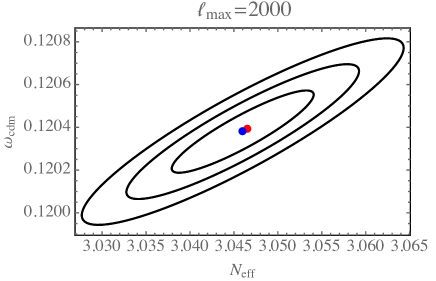
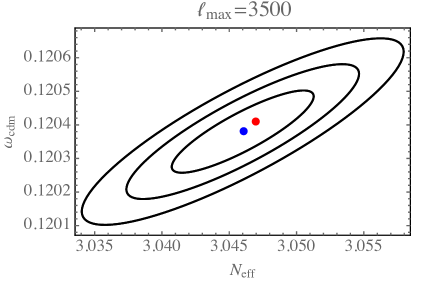
Figure 3: Fisher forecast (see Appendix D for details) for a cosmic variance limited survey. The blue (red) points show the shift in the best fit parameter for the dark matter density $\omega_{\text{cdm}}=h^{2}\Omega_{\text{cdm}}$ and the effective number of relativistic species $N_{\text{eff}}$ induced by the terms in Eqs. (6.13) and (6.14) (we consider vanishing primordial B-modes) using the linear power spectrum (using Halofit). The unshifted best fit value is covered by the blue point. The ellipses denote 1, 2 and 3 sigma contours. The parameters not shown in the panels are fixed to the fiducial cosmology. For both panels we consider B-mode up to $\ell_{\text{max}}=1500$ to be consistent with the conservative specifications of CMB-S4 Abazajian:2016yjj .

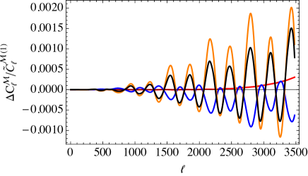
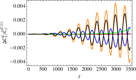
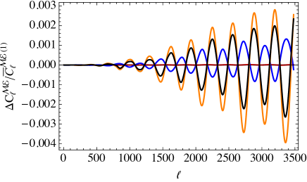
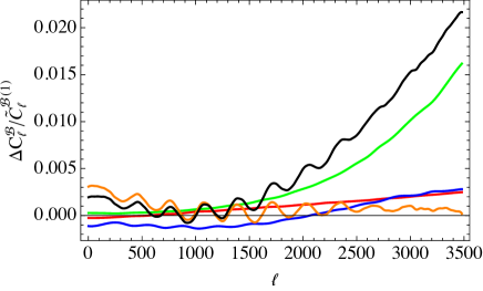
Figure 4: Higher order lensing contributions from the post-Born second group (red curves), post-Born third group (blue curves), LSS third group (orange curves), and rotation angle $\beta^{(2)}$ (green curves, contributions $(2,2)$). Black curves sum up the total correction. We consider the lensing CMB spectra for temperature (top left-panel), E-modes (top right-panel), cross TE spectra (bottom left-panel), where $\bar{C}_{\ell}^{\mathcal{M}\mathcal{E}(1)}=\sqrt{\frac{\left(\tilde{C}_{\ell}^{\mathcal{M}\mathcal{E}(1)}\right)^{2}+\tilde{C}^{\mathcal{M}(1)}_{\ell}\,\tilde{C}^{\mathcal{E}(1)}_{\ell}}{2}}$) and B-modes (bottom right-panel).

In Fig. 5 we present the ratio between these corrections and cosmic variance, $c^{X}_{\ell}$, $(\sigma^{X}_{\ell})^{2}$ given by

$$\sigma^{\mathcal{M}}_{\ell} = \sqrt{\frac{2}{2\ell+1}}\,C_{\ell}^{\mathcal{M}}\,,$$ (7.4)

$$\sigma^{\mathcal{E}}_{\ell} = \sqrt{\frac{2}{2\ell+1}}\,C_{\ell}^{\mathcal{E}}\,,$$ (7.5)

$$\sigma^{\mathcal{M}\mathcal{E}}_{\ell} = \sqrt{\frac{1}{2\ell+1}}\,\sqrt{\left(C_{\ell}^{\mathcal{M}\mathcal{E}}\right)^{2}+C^{\mathcal{M}}_{\ell}\,C^{\mathcal{E}}_{\ell}}\,,$$ (7.6)

$$\sigma^{\mathcal{B}}_{\ell} = \sqrt{\frac{2}{2\ell+1}}\,\tilde{C}_{\ell}^{\mathcal{B}(1)}\,.$$ (7.7)

Note that, for B-modes, we have taken into account the first order resummed correction since we consider no primordial gravitational wave, i.e the unlensed spectrum vanishes. Therefore, lensed B-modes do not have Gaussian statistics. For this reason its cosmic variance can be significantly larger than the one from Eq. (7.7) Smith:2006nk . Considering Gaussian variance also for B-modes, the corrections due to rotation alone are comparable to cosmic variance for $\ell\gtrsim 3500$, in contrast to all other spectra where all the corrections are always below that threshold. Moreover, the sum of all the effects can be even larger than cosmic variance at these multipoles, showing that higher-order lensing corrections to B-mode polarization at high multipoles have the best chance to be detectable.

Finally, in Fig. 6 we show the cumulative signal-to-noise ratio defined as

$$\left(\frac{S}{N}\right)^{2}=\sum_{\ell=30}^{\ell_{\rm max}}\left(\frac{\Delta C_{\ell}}{\sigma_{\ell}}\right)^{2}$$ (7.8)

where $\sigma_{\ell}$ are defined like in eqs. (7.4-7.7) but adding a noise contribution to the cosmic variance term, i.e. by replacing $C^{X}_{\ell}$ by $C^{X}_{\ell}+N^{X}_{\ell}$ where

$$N_{\ell}=(\Delta X)^{2}\exp\left(\frac{\ell\left(\ell+1\right)\theta^{2}_{\rm FWHM}}{8\ln 2}\right)$$ (7.9)

and $\Delta X=1\ \mu K\times\text{arcmin}$ for temperature, $\Delta X=\sqrt{2}\ \mu K\times\text{arcmin}$ for polarization and an angular resolution of $\theta_{\rm FWHM}=1$ arcmin. Our results are comparable with Ref. Fabbian:2017wfp . We predict a lower signal-to-noise ratio for the contribution to temperature anisotropies because we limit our analysis to $\ell_{\rm max}=3500$, while they have a smaller contribution for E-mode which seems due to non-perturbative effects we do not consider in our approach.

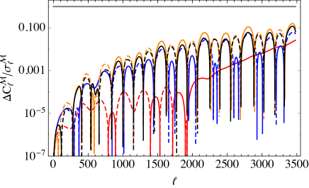
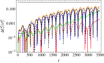
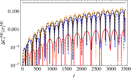
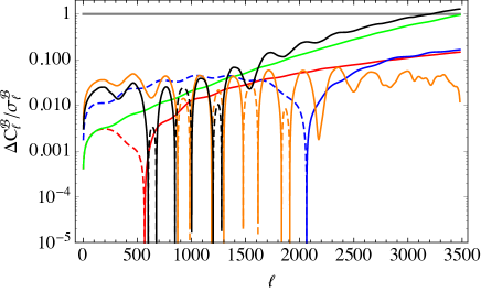
Figure 5: Comparison between next-to-leading order corrections and cosmic variance for the temperature (Eq. (7.4), top left-panel), E-modes (Eq. (7.5), top right-panel), TE cross correlation (Eq. (7.6), botto left-panel) and B-modes (Eq. (7.7), bottom right-panel). Red curves refer to post-Born second group, blue curves to post-Born third group, orange to LSS corrections third group and green curves represent the $(2,2)$ term of $\beta^{(2)}$. Dashed lines are negative values and the black lines trace the sum of all the terms.

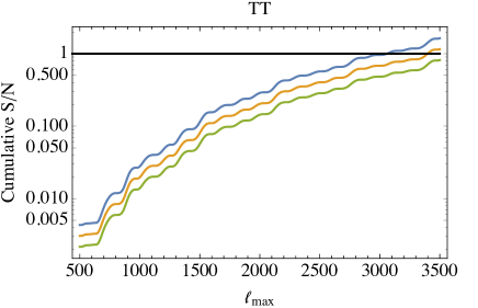
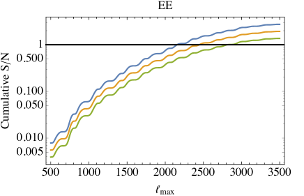
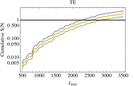
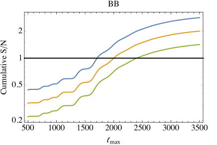
Figure 6: The signal-to-noise estimates of the total next to leading order effects for different sky coverage ($f_{\text{sky}}=0.25$, green curves, $f_{\text{sky}}=0.5$, orange curves and $f_{\text{sky}}=1$, blue curves) are shown as functions of $\mathcal{\ell}_{\text{max}}$. We consider the specifications of CMB S4 Abazajian:2016yjj : $1\ \mu K\times\text{arcmin}$ noise for temperature and $\sqrt{2}\mu K\times\text{arcmin}$ for polarization with an angular resolution of $1\ \text{arcmin}$.

8 Conclusions

In this paper we have computed all the next-to-leading order corrections to the CMB power spectra of temperature and polarization anisotropies from gravitational lensing of the photons along their path from the last scattering surface into our telescopes. We have found that most terms apart from those already taken into account in present codes Lewis:2006fu ; Blas:2011rf ; Lesgourgues:2011re are smaller than cosmic variance for a single $\ell$ mode. The only exception to this rule are the B-mode corrections at very high $\ell$. This can be understood from the fact that cosmic variance is proportional to the amplitude of the signal which is by far smallest for the B-modes. Nevertheless by considering the lensed B-modes as Gaussian, we may underestimate their variance Smith:2006nk .

Several of the terms calculated in this paper have already been determined before Pratten:2016dsm ; Marozzi:2016uob ; Lewis:2016tuj and our results are in good qualitative agreement, where comparable, with previous findings. This is a non-trivial consistency check, especially for Pratten:2016dsm ; Lewis:2016tuj which use quite different methods. Apart from rotation, the only other difference between our results and Lewis:2016tuj comes from the second group which has been neglected in Lewis:2016tuj . This leads to quite relevant differences for temperature at small scales ($\ell>3000$) and for the B-modes spectrum on all scales, whereas it does not change EE and TE spectra. The largest correction to the B-modes comes, however, from the rotation of the polarization direction which is new. It is very remarkable that our analytical results, including rotation, have been confirmed recently by N-body simulations with multiple-lens raytracing technique Fabbian:2017wfp ; Takahashi:2017hjr . Considering the different procedures, the level of agreement between the results is impressive.

It will be interesting to investigate whether these corrections are observable. Even though for an individual value $\ell$, the corrections are below cosmic variance, this is no longer so for sufficiently large bins of $\ell$’s, as we have shown in Fig. 6. Let us only note here, that the rotation of the polarisation is due to the vector-degree of freedom of the gravitational field, an effect like frame dragging. Its detection would therefore represent a highly non trivial test of general relativity, testing its elusive spin-1 sector. Recently, it has been proposed to measure this rotation with radio cosmic shear surveys Thomas:2016xhb .

But also the other terms are not negligible if a precision of 0.1% wants to be achieved as announced in Ref. Lesgourgues:2013bra . For example, for $\ell$ between 2000 and 2100, cosmic variance amounts to about 2.2%. Hence, as one easily infers from Figs. 4 and 5, our corrections with respect to the unlensed spectra are up to 0.1% for the E-polarization spectrum and for the T-E cross correlation, while they are at most 0.04% for the temperature anisotropy. For the B-polarization spectrum the correction is close to 0.5%.

It is clear that a systematic change even below cosmic variance can affect cosmological parameters and it has to be studied whether next-to-leading order corrections from lensing can indeed influence CMB parameter estimation in the future, this is the topic of an accompanying letter Marozzi:2016und . While, it is unlikely that the tiny corrections of the temperature will be relevant alone, parameters depending strongly on polarization can be affected. Indeed, in Marozzi:2016und we show how neglecting higher order lensing terms can lead to misinterpreting these corrections as a primordial tensor-to-scalar ratio of about $\mathcal{O}(10^{-3})$, and leads to a non-negligible shift of the estimated value of the effective number of relativistic species.

The fact that $\omega^{(2)}$ can significantly affect the CMB spectra has important consequences for delensing and lensing reconstruction. Those techniques, indeed, rely on the fact that lensing is mainly sourced by a scalar lensing potential, such that an (almost) exact remapping can be done between the intrinsic CMB maps at the last scattering surface and the lensed ones nowadays. However, if $\omega^{(2)}$ contributes significantly, new estimators for lensing reconstruction have to be developed. This task is highly non-trivial and requires a proper analysis. We shall postpone this investigation to future work.

However, independent of parameter estimation, detecting higher order corrections from CMB lensing would be extremely interesting and allow not only a handle on non-linear corrections to the gravitational potential, but also new tests of General Relativity on cosmological scales.

Appendix A $\mathcal{D}^{(i....)}(\boldsymbol{\ell})$ terms

In $\boldsymbol{\ell}$ space, and starting from the result of Marozzi:2016uob and of Sect. 5, we obtain the corresponding expressions to evaluate the lensing corrections to the CMB polarization anisotropies up to forth order:

$$\mathcal{D}^{(1)}(\boldsymbol{\ell}) = \frac{1}{2\pi}\int d^{2}x\,\theta^{a(1)}\nabla_{a}\mathcal{P}\,e^{i\boldsymbol{\ell}\cdot{\bf x}}$$ (A.1)

$$= -\frac{1}{\pi}\int d^{2}\ell_{2}\ \left[\left(\boldsymbol{\ell}-\boldsymbol{\ell}_{2}\right)\cdot\boldsymbol{\ell}_{2}\right]\int_{0}^{r_{s}}dr\frac{r_{s}-r}{r_{s}\,r}\,\Phi_{W}(r,\boldsymbol{\ell}-\boldsymbol{\ell}_{2})\left[\mathcal{E}(r_{s},\boldsymbol{\ell}_{2})+i\mathcal{B}(r_{s},\boldsymbol{\ell}_{2})\right]e^{-2i\varphi_{\ell_{2}}}\,,$$

$$\mathcal{D}^{(2)}(\boldsymbol{\ell}) = \frac{1}{2\pi}\int d^{2}x\,\theta^{a(2)}\nabla_{a}\mathcal{P}\,e^{i\boldsymbol{\ell}\cdot{\bf x}}$$ (A.2)

$$= -\frac{1}{\pi}\int d^{2}\ell_{2}\ \left[\left(\boldsymbol{\ell}-\boldsymbol{\ell}_{2}\right)\cdot\boldsymbol{\ell}_{2}\right]\int_{0}^{r_{s}}dr\frac{r_{s}-r}{r_{s}\,r}\,\Phi_{W}^{(2)}(r,\boldsymbol{\ell}-\boldsymbol{\ell}_{2})\left[\mathcal{E}(r_{s},\boldsymbol{\ell}_{2})+i\mathcal{B}(r_{s},\boldsymbol{\ell}_{2})\right]e^{-2i\varphi_{\ell_{2}}}$$

$$+\frac{1}{\pi^{2}}\int d^{2}\ell_{2}\ \int d^{2}\ell_{3}\ \,\left[\left(\boldsymbol{\ell}+\boldsymbol{\ell}_{2}-\boldsymbol{\ell}_{3}\right)\cdot\boldsymbol{\ell}_{3}\right]\,\left[\left(\boldsymbol{\ell}+\boldsymbol{\ell}_{2}-\boldsymbol{\ell}_{3}\right)\cdot\boldsymbol{\ell}_{2}\right]$$

$$\times\int_{0}^{r_{s}}dr\frac{r_{s}-r}{r_{s}\,r}\int_{0}^{r}dr^{\prime}\frac{r-r^{\prime}}{r\,r^{\prime}}\,\Phi_{W}(r,\boldsymbol{\ell}+\boldsymbol{\ell}_{2}-\boldsymbol{\ell}_{3})\bar{\Phi}_{W}(r^{\prime},\boldsymbol{\ell}_{2})\left[\mathcal{E}(r_{s},\boldsymbol{\ell}_{3})+i\mathcal{B}(r_{s},\boldsymbol{\ell}_{3})\right]e^{-2i\varphi_{\ell_{3}}}\,,$$

$$\mathcal{D}^{(11)}(\boldsymbol{\ell}) = \frac{1}{2\pi}\int d^{2}x\frac{1}{2}\theta^{a(1)}\theta^{b(1)}\nabla_{a}\nabla_{b}\mathcal{P}e^{i\boldsymbol{\ell}\cdot{\bf x}}$$ (A.3)

$$= \frac{1}{2}\frac{1}{\pi^{2}}\int d^{2}\ell_{2}\ \int d^{2}\ell_{3}\ \,\left[\left(\boldsymbol{\ell}+\boldsymbol{\ell}_{2}-\boldsymbol{\ell}_{3}\right)\cdot\boldsymbol{\ell}_{3}\right]\,\left(\boldsymbol{\ell}_{2}\cdot\boldsymbol{\ell}_{3}\right)\int_{0}^{r_{s}}dr\frac{r_{s}-r}{r_{s}\,r}\int_{0}^{r_{s}}dr^{\prime}\frac{r_{s}-r^{\prime}}{r_{s}\,r^{\prime}}$$

$$\qquad\times\Phi_{W}(r,\boldsymbol{\ell}+\boldsymbol{\ell}_{2}-\boldsymbol{\ell}_{3})\bar{\Phi}_{W}(r^{\prime},\boldsymbol{\ell}_{2})\left[\mathcal{E}(r_{s},\boldsymbol{\ell}_{3})+i\mathcal{B}(r_{s},\boldsymbol{\ell}_{3})\right]e^{-2i\varphi_{\ell_{3}}}\,,$$

$$\mathcal{D}^{(3)}(\boldsymbol{\ell}) = \frac{1}{2\pi}\int d^{2}x\,\theta^{a(3)}\nabla_{a}\mathcal{P}\,e^{i\boldsymbol{\ell}\cdot{\bf x}}$$ (A.4)

$$= -\frac{1}{\pi}\int d^{2}\ell_{2}\ \left[\left(\boldsymbol{\ell}-\boldsymbol{\ell}_{2}\right)\cdot\boldsymbol{\ell}_{2}\right]\int_{0}^{r_{s}}dr\frac{r_{s}-r}{r_{s}\,r}\,\Phi_{W}^{(3)}(r,\boldsymbol{\ell}-\boldsymbol{\ell}_{2})\left[\mathcal{E}(r_{s},\boldsymbol{\ell}_{2})+i\mathcal{B}(r_{s},\boldsymbol{\ell}_{2})\right]e^{-2i\varphi_{\ell_{2}}}$$

$$+\frac{1}{\pi^{2}}\int d^{2}\ell_{2}\ \int d^{2}\ell_{3}\ \,\left[\left(\boldsymbol{\ell}+\boldsymbol{\ell}_{2}-\boldsymbol{\ell}_{3}\right)\cdot\boldsymbol{\ell}_{3}\right]\,\left[\left(\boldsymbol{\ell}+\boldsymbol{\ell}_{2}-\boldsymbol{\ell}_{3}\right)\cdot\boldsymbol{\ell}_{2}\right]\int_{0}^{r_{s}}dr^{\prime}\frac{r_{s}-r}{r_{s}\,r}\int_{0}^{r}dr^{\prime}\frac{r-r^{\prime}}{r\,r^{\prime}}\,$$

$$\times\left[\Phi_{W}(r,\boldsymbol{\ell}+\boldsymbol{\ell}_{2}-\boldsymbol{\ell}_{3})\bar{\Phi}_{W}^{(2)}(r^{\prime},\boldsymbol{\ell}_{2})+\Phi_{W}^{(2)}(r,\boldsymbol{\ell}+\boldsymbol{\ell}_{2}-\boldsymbol{\ell}_{3})\bar{\Phi}_{W}(r^{\prime},\boldsymbol{\ell}_{2})\right]\left[\mathcal{E}(r_{s},\boldsymbol{\ell}_{3})+i\mathcal{B}(r_{s},\boldsymbol{\ell}_{3})\right]e^{-2i\varphi_{\ell_{3}}}$$

$$-\frac{1}{\pi^{3}}\int d^{2}\ell_{2}\ \int d^{2}\ell_{3}\ \int d^{2}\ell_{4}\ \left\{\left[\left(\boldsymbol{\ell}-\boldsymbol{\ell}_{2}-\boldsymbol{\ell}_{3}-\boldsymbol{\ell}_{4}\right)\cdot\boldsymbol{\ell}_{4}\right]\,\left[\left(\boldsymbol{\ell}-\boldsymbol{\ell}_{2}-\boldsymbol{\ell}_{3}-\boldsymbol{\ell}_{4}\right)\cdot\boldsymbol{\ell}_{2}\right]\right.$$

$$\left.\times\left(\boldsymbol{\ell}_{2}\cdot\boldsymbol{\ell}_{3}\right)\int_{0}^{r_{s}}dr\frac{r_{s}-r}{r_{s}\,r}\int_{0}^{r}dr^{\prime}\frac{r-r^{\prime}}{r\,r^{\prime}}\int_{0}^{r^{\prime}}dr^{\prime\prime}\frac{r^{\prime}-r^{\prime\prime}}{r^{\prime}\,r^{\prime\prime}}\right.$$

$$\times\,\Phi_{W}(r,\boldsymbol{\ell}-\boldsymbol{\ell}_{2}-\boldsymbol{\ell}_{3}-\boldsymbol{\ell}_{4})\Phi_{W}(r^{\prime},\boldsymbol{\ell}_{2})\Phi_{W}(r^{\prime\prime},\boldsymbol{\ell}_{3})\left[\mathcal{E}(r_{s},\boldsymbol{\ell}_{4})+i\mathcal{B}(r_{s},\boldsymbol{\ell}_{4})\right]e^{-2i\varphi_{\ell_{4}}}$$

$$\left.+\frac{1}{2}\left[\left(\boldsymbol{\ell}-\boldsymbol{\ell}_{2}-\boldsymbol{\ell}_{3}-\boldsymbol{\ell}_{4}\right)\cdot\boldsymbol{\ell}_{4}\right]\,\left[\left(\boldsymbol{\ell}-\boldsymbol{\ell}_{2}-\boldsymbol{\ell}_{3}-\boldsymbol{\ell}_{4}\right)\cdot\boldsymbol{\ell}_{2}\right]\,\left[\left(\boldsymbol{\ell}-\boldsymbol{\ell}_{2}-\boldsymbol{\ell}_{3}-\boldsymbol{\ell}_{4}\right)\cdot\boldsymbol{\ell}_{3}\right]\right.$$

$$\left.\times\int_{0}^{r_{s}}dr\frac{r_{s}-r}{r_{s}\,r}\int_{0}^{r}dr^{\prime}\frac{r-r^{\prime}}{r\,r^{\prime}}\,\int_{0}^{r}dr^{\prime\prime}\frac{r-r^{\prime\prime}}{r\,r^{\prime\prime}}\right.$$

$$\left.\times\,\Phi_{W}(r,\boldsymbol{\ell}-\boldsymbol{\ell}_{2}-\boldsymbol{\ell}_{3}-\boldsymbol{\ell}_{4})\Phi_{W}(r^{\prime},\boldsymbol{\ell}_{2})\Phi_{W}(r^{\prime\prime},\boldsymbol{\ell}_{3})\left[\mathcal{E}(r_{s},\boldsymbol{\ell}_{4})+i\mathcal{B}(r_{s},\boldsymbol{\ell}_{4})\right]e^{-2i\varphi_{\ell_{4}}}\right\}\,,$$

$$\mathcal{D}^{(12)}(\boldsymbol{\ell}) = \frac{1}{2\pi}\int d^{2}x\,\theta^{a(1)}\theta^{b(2)}\nabla_{a}\nabla_{b}\mathcal{P}\,e^{i\boldsymbol{\ell}_{\cdot}{\bf x}}$$ (A.5)

$$= \frac{1}{\pi^{2}}\int d^{2}\ell_{2}\ \int d^{2}\ell_{3}\ \,\left[\left(\boldsymbol{\ell}+\boldsymbol{\ell}_{2}-\boldsymbol{\ell}_{3}\right)\cdot\boldsymbol{\ell}_{3}\right]\,\left(\boldsymbol{\ell}_{2}\cdot\boldsymbol{\ell}_{3}\right)\int_{0}^{r_{s}}dr\frac{r_{s}-r}{r_{s}\,r}$$

$$\times\int_{0}^{r_{s}}dr^{\prime}\frac{r_{s}-r^{\prime}}{r_{s}\,r^{\prime}}\Phi_{W}(r,\boldsymbol{\ell}+\boldsymbol{\ell}_{2}-\boldsymbol{\ell}_{3})\bar{\Phi}^{(2)}_{W}(r^{\prime},\boldsymbol{\ell}_{2})\,\left[\mathcal{E}(r_{s},\boldsymbol{\ell}_{3})+i\mathcal{B}(r_{s},\boldsymbol{\ell}_{3})\right]e^{-2i\varphi_{\ell_{3}}}$$

$$-\frac{1}{\pi^{3}}\int d^{2}\ell_{2}\ \int d^{2}\ell_{3}\ \int d^{2}\ell_{4}\ \left[\left(\boldsymbol{\ell}-\boldsymbol{\ell}_{2}-\boldsymbol{\ell}_{3}-\boldsymbol{\ell}_{4}\right)\cdot\boldsymbol{\ell}_{4}\right]\,\left(\boldsymbol{\ell}_{4}\cdot\boldsymbol{\ell}_{2}\right)\,\left(\boldsymbol{\ell}_{3}\cdot\boldsymbol{\ell}_{2}\right)$$

$$\times\int_{0}^{r_{s}}dr\frac{r_{s}-r}{r_{s}\,r}\int_{0}^{r_{s}}dr^{\prime}\frac{r_{s}-r^{\prime}}{r_{s}\,r^{\prime}}\int_{0}^{r^{\prime}}dr^{\prime\prime}\frac{r^{\prime}-r^{\prime\prime}}{r^{\prime}\,r^{\prime\prime}}\,\Phi_{W}(r,\boldsymbol{\ell}-\boldsymbol{\ell}_{2}-\boldsymbol{\ell}_{3}-\boldsymbol{\ell}_{4})\,$$

$$\times\Phi_{W}(r^{\prime},\boldsymbol{\ell}_{2})\Phi_{W}(r^{\prime\prime},\boldsymbol{\ell}_{3})\left[\mathcal{E}(r_{s},\boldsymbol{\ell}_{4})+i\mathcal{B}(r_{s},\boldsymbol{\ell}_{4})\right]e^{-2i\varphi_{\ell_{4}}}$$

$$\mathcal{D}^{(111)}(\boldsymbol{\ell}) = \frac{1}{2\pi}\int d^{2}x\frac{1}{6}\,\theta^{a(1)}\theta^{b(1)}\theta^{c(1)}\nabla_{a}\nabla_{b}\nabla_{c}\mathcal{P}\,e^{i\boldsymbol{\ell}\cdot{\bf x}}$$ (A.6)

$$= -\frac{1}{6}\frac{1}{\pi^{3}}\int d^{2}\ell_{2}\ \int d^{2}\ell_{3}\ \int d^{2}\ell_{4}\ \left[\left(\boldsymbol{\ell}-\boldsymbol{\ell}_{2}-\boldsymbol{\ell}_{3}-\boldsymbol{\ell}_{4}\right)\cdot\boldsymbol{\ell}_{4}\right]\,\left(\boldsymbol{\ell}_{2}\cdot\boldsymbol{\ell}_{4}\right)\,\left(\boldsymbol{\ell}_{3}\cdot\boldsymbol{\ell}_{4}\right)$$

$$\times\int_{0}^{r_{s}}dr\frac{r_{s}-r}{r_{s}\,r}\,\int_{0}^{r_{s}}dr^{\prime}\frac{r_{s}-r^{\prime}}{r_{s}\,r^{\prime}}\,\int_{0}^{r_{s}}dr^{\prime\prime}\frac{r_{s}-r^{\prime\prime}}{r_{s}\,r^{\prime\prime}}\,\Phi_{W}(r,\boldsymbol{\ell}-\boldsymbol{\ell}_{2}-\boldsymbol{\ell}_{3}-\boldsymbol{\ell}_{4})$$

$$\times\Phi_{W}(r^{\prime},\boldsymbol{\ell}_{2})\Phi_{W}(r^{\prime\prime},\boldsymbol{\ell}_{3})\left[\mathcal{E}(r_{s},\boldsymbol{\ell}_{4})+i\mathcal{B}(r_{s},\boldsymbol{\ell}_{4})\right]e^{-2i\varphi_{\ell_{4}}}\,,$$

$$\mathcal{D}^{(22)}(\boldsymbol{\ell}) = \frac{1}{2\pi}\int d^{2}x\,\frac{1}{2}\,\theta^{a(2)}\theta^{b(2)}\nabla_{a}\nabla_{b}\mathcal{P}\,e^{i\boldsymbol{\ell}_{\cdot}{\bf x}}$$ (A.7)

$$= \frac{1}{2}\frac{1}{\pi^{2}}\int d^{2}\ell_{2}\ \int d^{2}\ell_{3}\ \,\left[\left(\boldsymbol{\ell}+\boldsymbol{\ell}_{2}-\boldsymbol{\ell}_{3}\right)\cdot\boldsymbol{\ell}_{3}\right]\,\left(\boldsymbol{\ell}_{2}\cdot\boldsymbol{\ell}_{3}\right)\int_{0}^{r_{s}}dr\frac{r_{s}-r}{r_{s}\,r}\int_{0}^{r_{s}}dr^{\prime}\frac{r_{s}-r^{\prime}}{r_{s}\,r^{\prime}}$$

$$\times\Phi_{W}^{(2)}(r,\boldsymbol{\ell}+\boldsymbol{\ell}_{2}-\boldsymbol{\ell}_{3})\bar{\Phi}_{W}^{(2)}(r^{\prime},\boldsymbol{\ell}_{2})\left[\mathcal{E}(r_{s},\boldsymbol{\ell}_{3})+i\mathcal{B}(r_{s},\boldsymbol{\ell}_{3})\right]e^{-2i\varphi_{\ell_{3}}}$$

$$-\frac{1}{\pi^{3}}\int d^{2}\ell_{2}\ \int d^{2}\ell_{3}\ \int d^{2}\ell_{4}\ \left[\left(\boldsymbol{\ell}-\boldsymbol{\ell}_{2}-\boldsymbol{\ell}_{3}-\boldsymbol{\ell}_{4}\right)\cdot\boldsymbol{\ell}_{4}\right]\,\left(\boldsymbol{\ell}_{4}\cdot\boldsymbol{\ell}_{2}\right)\,\left(\boldsymbol{\ell}_{3}\cdot\boldsymbol{\ell}_{2}\right)\int_{0}^{r_{s}}dr\frac{r_{s}-r}{r_{s}\,r}\int_{0}^{r_{s}}dr^{\prime}\frac{r_{s}-r^{\prime}}{r_{s}\,r^{\prime}},$$

$$\times\,\int_{0}^{r^{\prime}}dr^{\prime\prime}\frac{r^{\prime}-r^{\prime\prime}}{r^{\prime}\,r^{\prime\prime}}\Phi_{W}^{(2)}(r,\boldsymbol{\ell}-\boldsymbol{\ell}_{2}-\boldsymbol{\ell}_{3}-\boldsymbol{\ell}_{4})\Phi_{W}(r^{\prime},\boldsymbol{\ell}_{2})\Phi_{W}(r^{\prime\prime},\boldsymbol{\ell}_{3})\left[\mathcal{E}(r_{s},\boldsymbol{\ell}_{4})+i\mathcal{B}(r_{s},\boldsymbol{\ell}_{4})\right]e^{-2i\varphi_{\ell_{4}}}$$

$$-\frac{1}{2}\frac{1}{\pi^{4}}\int d^{2}\ell_{2}\ \int d^{2}\ell_{3}\ \int d^{2}\ell_{4}\ \int d^{2}\ell_{5}\ \left[\left(\boldsymbol{\ell}-\boldsymbol{\ell}_{2}-\boldsymbol{\ell}_{3}-\boldsymbol{\ell}_{4}-\boldsymbol{\ell}_{5}\right)\cdot\boldsymbol{\ell}_{5}\right]$$

$$\times\left[\left(\boldsymbol{\ell}-\boldsymbol{\ell}_{2}-\boldsymbol{\ell}_{3}-\boldsymbol{\ell}_{4}-\boldsymbol{\ell}_{5}\right)\cdot\boldsymbol{\ell}_{2}\right]\left(\boldsymbol{\ell}_{5}\cdot\boldsymbol{\ell}_{3}\right)\,\left(\boldsymbol{\ell}_{3}\cdot\boldsymbol{\ell}_{4}\right)\int_{0}^{r_{s}}dr\frac{r_{s}-r}{r_{s}\,r}\int_{0}^{r}dr^{\prime}\frac{r-r^{\prime}}{r\,r^{\prime}}\,\int_{0}^{r_{s}}dr^{\prime\prime}\frac{r_{s}-r^{\prime\prime}}{r_{s}\,r^{\prime\prime}}\int_{0}^{r^{\prime\prime}}dr^{\prime\prime\prime}\frac{r^{\prime\prime}-r^{\prime\prime\prime}}{r^{\prime\prime}\,r^{\prime\prime\prime}}$$

$$\times\,\Phi_{W}(r,\boldsymbol{\ell}-\boldsymbol{\ell}_{2}-\boldsymbol{\ell}_{3}-\boldsymbol{\ell}_{4}-\boldsymbol{\ell}_{5})\Phi_{W}(r^{\prime},\boldsymbol{\ell}_{2})\Phi_{W}(r^{\prime\prime},\boldsymbol{\ell}_{3})\Phi_{W}(r^{\prime\prime\prime},\boldsymbol{\ell}_{4})\left[\mathcal{E}(r_{s},\boldsymbol{\ell}_{5})+i\mathcal{B}(r_{s},\boldsymbol{\ell}_{5})\right]e^{-2i\varphi_{\ell_{5}}}\,,$$

$$\mathcal{D}^{(13)}(\boldsymbol{\ell}) = \frac{1}{2\pi}\int d^{2}x\,\theta^{a(1)}\theta^{b(3)}\nabla_{a}\nabla_{b}\mathcal{P}\,e^{i\boldsymbol{\ell}\cdot{\bf x}}$$ (A.8)

$$= \frac{1}{\pi^{2}}\int d^{2}\ell_{2}\ \int d^{2}\ell_{3}\ \,\left[\left(\boldsymbol{\ell}+\boldsymbol{\ell}_{2}-\boldsymbol{\ell}_{3}\right)\cdot\boldsymbol{\ell}_{3}\right]\,\left(\boldsymbol{\ell}_{2}\cdot\boldsymbol{\ell}_{3}\right)\int_{0}^{r_{s}}dr\frac{r_{s}-r}{r_{s}\,r}\int_{0}^{r_{s}}dr^{\prime}\frac{r_{s}-r^{\prime}}{r_{s}\,r^{\prime}}$$

$$\times\Phi_{W}(r,\boldsymbol{\ell}+\boldsymbol{\ell}_{2}-\boldsymbol{\ell}_{3})\bar{\Phi}^{(3)}_{W}(r^{\prime},\boldsymbol{\ell}_{3})\left[\mathcal{E}(r_{s},\boldsymbol{\ell}_{3})+i\mathcal{B}(r_{s},\boldsymbol{\ell}_{3})\right]e^{-2i\varphi_{\ell_{3}}}$$

$$-\frac{1}{\pi^{3}}\int d^{2}\ell_{2}\ \int d^{2}\ell_{3}\ \int d^{2}\ell_{4}\ \left[\left(\boldsymbol{\ell}-\boldsymbol{\ell}_{2}-\boldsymbol{\ell}_{3}-\boldsymbol{\ell}_{4}\right)\cdot\boldsymbol{\ell}_{4}\right]\,\left(\boldsymbol{\ell}_{4}\cdot\boldsymbol{\ell}_{2}\right)\,\left(\boldsymbol{\ell}_{3}\cdot\boldsymbol{\ell}_{2}\right)$$

$$\times\int_{0}^{r_{s}}dr\frac{r_{s}-r}{r_{s}\,r}\int_{0}^{r_{s}}dr^{\prime}\frac{r_{s}-r^{\prime}}{r_{s}\,r^{\prime}}\int_{0}^{r^{\prime}}dr^{\prime\prime}\frac{r^{\prime}-r^{\prime\prime}}{r^{\prime}\,r^{\prime\prime}}\,\Phi_{W}(r,\boldsymbol{\ell}-\boldsymbol{\ell}_{2}-\boldsymbol{\ell}_{3}-\boldsymbol{\ell}_{4})\left[\Phi_{W}(r^{\prime},\boldsymbol{\ell}_{2})\Phi^{(2)}_{W}(r^{\prime\prime},\boldsymbol{\ell}_{3})\right.$$

$$\left.+\Phi_{W}^{(2)}(r^{\prime},\boldsymbol{\ell}_{2})\Phi_{W}(r^{\prime\prime},\boldsymbol{\ell}_{3})\right]\left[\mathcal{E}(r_{s},\boldsymbol{\ell}_{4})+i\mathcal{B}(r_{s},\boldsymbol{\ell}_{4})\right]e^{-2i\varphi_{\ell_{4}}}$$

$$-\frac{1}{\pi^{4}}\int d^{2}\ell_{2}\ \int d^{2}\ell_{3}\ \int d^{2}\ell_{4}\ \int d^{2}\ell_{5}\ \left\{\left[\left(\boldsymbol{\ell}-\boldsymbol{\ell}_{2}-\boldsymbol{\ell}_{3}-\boldsymbol{\ell}_{4}-\boldsymbol{\ell}_{5}\right)\cdot\boldsymbol{\ell}_{5}\right]\,\left(\boldsymbol{\ell}_{2}\cdot\boldsymbol{\ell}_{5}\right)\right.\left(\boldsymbol{\ell}_{2}\cdot\boldsymbol{\ell}_{3}\right)\left(\boldsymbol{\ell}_{3}\cdot\boldsymbol{\ell}_{4}\right)$$

$$\times\int_{0}^{r_{s}}dr\frac{r_{s}-r}{r_{s}\,r}\int_{0}^{r_{s}}dr^{\prime}\frac{r_{s}-r^{\prime}}{r_{s}\,r^{\prime}}\int_{0}^{r^{\prime}}dr^{\prime\prime}\frac{r^{\prime}-r^{\prime\prime}}{r^{\prime}\,r^{\prime\prime}}\int_{0}^{r^{\prime\prime}}dr^{\prime\prime\prime}\frac{r^{\prime\prime}-r^{\prime\prime\prime}}{r^{\prime\prime}\,r^{\prime\prime\prime}}\Phi_{W}(r,\boldsymbol{\ell}-\boldsymbol{\ell}_{2}-\boldsymbol{\ell}_{3}-\boldsymbol{\ell}_{4}-\boldsymbol{\ell}_{5})\Phi_{W}(r^{\prime},\boldsymbol{\ell}_{2})$$

$$\times\Phi_{W}(r^{\prime\prime},\boldsymbol{\ell}_{3})\Phi_{W}(r^{\prime\prime\prime},\boldsymbol{\ell}_{4})\left[\mathcal{E}(r_{s},\boldsymbol{\ell}_{5})+i\mathcal{B}(r_{s},\boldsymbol{\ell}_{5})\right]e^{-2i\varphi_{\ell_{5}}}$$

$$+\frac{1}{2}\left[\left(\boldsymbol{\ell}-\boldsymbol{\ell}_{2}-\boldsymbol{\ell}_{3}-\boldsymbol{\ell}_{4}-\boldsymbol{\ell}_{5}\right)\cdot\boldsymbol{\ell}_{5}\right]\,\left(\boldsymbol{\ell}_{2}\cdot\boldsymbol{\ell}_{5}\right)\left(\boldsymbol{\ell}_{2}\cdot\boldsymbol{\ell}_{3}\right)\,\left(\boldsymbol{\ell}_{2}\cdot\boldsymbol{\ell}_{4}\right)\int_{0}^{r_{s}}dr\frac{r_{s}-r}{r_{s}\,r}\,\int_{0}^{r_{s}}dr^{\prime}\frac{r_{s}-r^{\prime}}{r_{s}\,r^{\prime}}\int_{0}^{r^{\prime}}dr^{\prime\prime}\frac{r^{\prime}-r^{\prime\prime}}{r^{\prime}\,r^{\prime\prime}}\,$$

$$\left.\times\,\int_{0}^{r^{\prime}}dr^{\prime\prime\prime}\frac{r^{\prime}-r^{\prime\prime\prime}}{r^{\prime}\,r^{\prime\prime\prime}}\Phi_{W}(r,\boldsymbol{\ell}-\boldsymbol{\ell}_{2}-\boldsymbol{\ell}_{3}-\boldsymbol{\ell}_{4}-\boldsymbol{\ell}_{5})\Phi_{W}(r^{\prime},\boldsymbol{\ell}_{2})\Phi_{W}(r^{\prime\prime},\boldsymbol{\ell}_{3})\Phi_{W}(r^{\prime\prime\prime},\boldsymbol{\ell}_{4})\right.$$

$$\left.\times\,\left[\mathcal{E}(r_{s},\boldsymbol{\ell}_{5})+i\mathcal{B}(r_{s},\boldsymbol{\ell}_{5})\right]e^{-2i\varphi_{\ell_{5}}}\right\}\,,$$

$$\mathcal{D}^{(1111)}(\boldsymbol{\ell}) = \frac{1}{2\pi}\int d^{2}x\,\frac{1}{24}\,\theta^{a(1)}\theta^{b(1)}\theta^{c(1)}\theta^{d(1)}\nabla_{a}\nabla_{b}\nabla_{c}\nabla_{d}\mathcal{P}\,e^{i\boldsymbol{\ell}\cdot{\bf x}}$$ (A.9)

$$= -\frac{1}{24}\frac{1}{\pi^{4}}\int d^{2}\ell_{2}\ \int d^{2}\ell_{3}\ \int d^{2}\ell_{4}\ \int d^{2}\ell_{5}\ \left[\left(\boldsymbol{\ell}-\boldsymbol{\ell}_{2}-\boldsymbol{\ell}_{3}-\boldsymbol{\ell}_{4}-\boldsymbol{\ell}_{5}\right)\cdot\boldsymbol{\ell}_{5}\right]$$

$$\times\left(\boldsymbol{\ell}_{2}\cdot\boldsymbol{\ell}_{5}\right)\,\left(\boldsymbol{\ell}_{3}\cdot\boldsymbol{\ell}_{5}\right)\,\left(\boldsymbol{\ell}_{4}\cdot\boldsymbol{\ell}_{5}\right)\int_{0}^{r_{s}}dr\frac{r_{s}-r}{r_{s}\,r}\int_{0}^{r_{s}}dr^{\prime}\frac{r_{s}-r^{\prime}}{r_{s}\,r^{\prime}}\,\int_{0}^{r_{s}}dr^{\prime\prime}\frac{r_{s}-r^{\prime\prime}}{r_{s}\,r^{\prime\prime}}\int_{0}^{r_{s}}dr^{\prime\prime\prime}\frac{r_{s}-r^{\prime\prime\prime}}{r_{s}\,r^{\prime\prime\prime}}$$

$$\times\Phi_{W}(r,\boldsymbol{\ell}-\boldsymbol{\ell}_{2}-\boldsymbol{\ell}_{3}-\boldsymbol{\ell}_{4}-\boldsymbol{\ell}_{5})\Phi_{W}(r^{\prime},\boldsymbol{\ell}_{2})\Phi_{W}(r^{\prime\prime},\boldsymbol{\ell}_{3})\Phi_{W}(r^{\prime\prime\prime},\boldsymbol{\ell}_{4})\left[\mathcal{E}(r_{s},\boldsymbol{\ell}_{5})+i\mathcal{B}(r_{s},\boldsymbol{\ell}_{5})\right]e^{-2i\varphi_{\ell_{5}}}\,.$$

We do not write the terms $\mathcal{D}^{(4)}$ and $\mathcal{D}^{(112)}$ because the associated contributions to the angular power spectra of lensed polarization tensor vanish as a consequence of statistical isotropy (see Sect. 3).

Appendix B Lensed angular power spectra for polarization

Following Sect. 3 and Marozzi:2016uob we now present the evaluation of the next-to-leading order corrections to E- and B-mode polarization spectra. More details are given in Ref. Marozzi:2016uob , where we compute, however, only the temperature anisotropy spectrum. Therefore, for completeness, we repeat the procedure here for the polarization spectra and for the temperature polarization cross-correlation.

B.1 Results $\tilde{C}_{\ell}^{\mathcal{E}\mathcal{M}}$

Let us begin by evaluating the lensed cross-correlation, $\tilde{C}_{\ell}^{\mathcal{E}\mathcal{M}}$. Up to next to next-to-leading order, we have

$$-e^{2i\varphi_{\ell}}\langle\tilde{\mathcal{P}}(\boldsymbol{\ell})\bar{\tilde{\mathcal{M}}}(\boldsymbol{\ell}^{\prime})\rangle=\delta(\boldsymbol{\ell}-\boldsymbol{\ell}^{\prime})\tilde{C}_{\ell}^{\mathcal{E}\mathcal{M}}$$ (B.1)

$$= \delta(\boldsymbol{\ell}-\boldsymbol{\ell}^{\prime}){C}_{\ell}^{\mathcal{E}\mathcal{M}}-e^{2i\varphi_{\ell}}\langle\mathcal{D}(\boldsymbol{\ell})\bar{\mathcal{A}}(\boldsymbol{\ell}\,^{\prime})\rangle\,,$$

where $\mathcal{A}(\boldsymbol{\ell})$ is given in Eq. (3.19) and we introduce

$$\mathcal{D}(\boldsymbol{\ell}) = \mathcal{D}^{(0)}(\boldsymbol{\ell})+\sum_{i=1}^{4}\mathcal{D}^{(i)}(\boldsymbol{\ell})+\sum_{\begin{subarray}{c}i+j\leq 4\\ 1\leq i\leq j\end{subarray}}\mathcal{D}^{(ij)}(\boldsymbol{\ell})$$ (B.2)

$$+\sum_{\begin{subarray}{c}i+j+k\leq 4\\ 1\leq i\leq j\leq k\end{subarray}}\mathcal{D}^{(ijk)}(\boldsymbol{\ell})+\mathcal{D}^{(1111)}(\boldsymbol{\ell})\,,$$

the 2d Fourier transforms of $\mathcal{D}(x^{a})$ defined in Eq. (2.4). We now introduce the expectation values $\hat{F}_{\ell}^{(i\ldots)}$ and $\hat{F}_{\ell}^{(i\ldots,\,j\ldots)}$ by

$$\delta\left(\boldsymbol{\ell}-\boldsymbol{\ell}\,^{\prime}\right)\hat{F}_{\ell}^{(ij\ldots,ij\ldots)} = \langle\mathcal{D}^{(ij\ldots)}(\boldsymbol{\ell})\bar{\mathcal{A}}^{(ij\ldots)}(\boldsymbol{\ell}\,^{\prime})\rangle\,,$$

$$\delta\left(\boldsymbol{\ell}-\boldsymbol{\ell}\,^{\prime}\right)\hat{F}_{\ell}^{(ij\ldots,i^{\prime}j^{\prime}\ldots)} = \langle\mathcal{D}^{(ij\ldots)}(\boldsymbol{\ell})\bar{\mathcal{A}}^{(i^{\prime}j^{\prime}\ldots)}(\boldsymbol{\ell}\,^{\prime})\rangle$$ (B.3)

$$+ \langle\mathcal{D}^{(i^{\prime}j^{\prime}\ldots)}(\boldsymbol{\ell})\bar{\mathcal{A}}^{(ij\ldots)}(\boldsymbol{\ell}\,^{\prime})\rangle\,,\ \ \$$

where the last definition applies when the coefficients $(ij\ldots)$ and $(i^{\prime}j^{\prime}\ldots)$ are not identical. The Dirac delta function $\delta\left(\boldsymbol{\ell}-\boldsymbol{\ell}\,^{\prime}\right)$ is a consequence of statistical isotropy. By omitting terms of higher than fourth order in the Weyl potential and terms that vanish as a consequence of Wick’s theorem (odd number of Weyl potentials), we obtain

$$\tilde{C}^{\mathcal{E}\mathcal{M}}_{\ell} = C^{{\mathcal{E}\mathcal{M}}}_{\ell}+F_{\ell}^{(0,2)}+F_{\ell}^{(0,11)}+F_{\ell}^{(1,1)}+F_{\ell}^{(0,4)}+F_{\ell}^{(0,13)}$$ (B.4)

$$+ F_{\ell}^{(0,22)}+F_{\ell}^{(0,112)}+F_{\ell}^{(0,1111)}+F_{\ell}^{(1,3)}+F_{\ell}^{(2,2)}$$

$$+ F_{\ell}^{(1,12)}+F_{\ell}^{(1,111)}+F_{\ell}^{(2,11)}+F_{\ell}^{(11,11)}\,,$$

where ${F}_{\ell}^{(i\ldots,j\ldots)}=-e^{2i\varphi_{\ell}}\hat{F}_{\ell}^{(i\ldots,j\ldots)}$.

As the terms $\mathcal{D}^{(i\ldots)}$ are simply related to the $\mathcal{A}^{(i\ldots)}$ terms, also the terms $\hat{F}_{\ell}^{(i\ldots,\,j\ldots)}$ can be easily evaluated from the $C_{\ell}^{(i\ldots,\,j\ldots)}$. In fact, using Eq. (3.13) and the results for the $\mathcal{D}^{(i\ldots)}$ and $\mathcal{A}^{(i\ldots)}$ terms (see Sect. 5, Appendix A and Marozzi:2016uob ), one finds that the $\hat{F}_{\ell}^{(i\ldots,\,j\ldots)}$ are given by the $C_{\ell}^{(i\ldots,\,j\ldots)}$ simply by substituting

$$C_{\ell}^{\mathcal{M}}(z_{s})\quad\rightarrow\quad-C_{\ell}^{\mathcal{E}\mathcal{M}}(z_{s})e^{-2i\varphi_{\ell}}\,.$$ (B.5)

The substitution is performed for any $C_{\ell}^{\mathcal{M}}(z_{s})$ inside and outside the integrals.

B.2 Results $\tilde{C}_{\ell}^{\mathcal{E}}+\tilde{C}_{\ell}^{\mathcal{B}}$

Let us also evaluate $\tilde{C}_{\ell}^{\mathcal{E}}+\tilde{C}_{\ell}^{\mathcal{B}}$. Proceeding as in the previous subsection we have

$$\langle\tilde{\mathcal{P}}(\boldsymbol{\ell})\bar{\tilde{\mathcal{P}}}(\boldsymbol{\ell}^{\prime})\rangle = \delta(\boldsymbol{\ell}-\boldsymbol{\ell}^{\prime})\left[\tilde{C}_{\ell}^{\mathcal{E}}+\tilde{C}_{\ell}^{\mathcal{B}}\right]$$ (B.6)

$$= \delta(\boldsymbol{\ell}-\boldsymbol{\ell}^{\prime})\left[{C}_{\ell}^{\mathcal{E}}+{C}_{\ell}^{\mathcal{B}}\right]+\langle\mathcal{D}(\boldsymbol{\ell})\bar{\mathcal{D}}(\boldsymbol{\ell}\,^{\prime})\rangle\,.\ \ \ \$$

We now introduce $M_{\ell}^{(i\ldots)}$ and $M_{\ell}^{(i\ldots,\,j\ldots)}$ given by

$$\delta\left(\boldsymbol{\ell}-\boldsymbol{\ell}\,^{\prime}\right)M_{\ell}^{(ij\ldots,ij\ldots)} = \langle\mathcal{D}^{(ij\ldots)}(\boldsymbol{\ell})\bar{\mathcal{D}}^{(ij\ldots)}(\boldsymbol{\ell}\,^{\prime})\rangle\,,$$

$$\delta\left(\boldsymbol{\ell}-\boldsymbol{\ell}\,^{\prime}\right)M_{\ell}^{(ij\ldots,i^{\prime}j^{\prime}\ldots)} = \langle\mathcal{D}^{(ij\ldots)}(\boldsymbol{\ell})\bar{\mathcal{D}}^{(i^{\prime}j^{\prime}\ldots)}(\boldsymbol{\ell}\,^{\prime})\rangle$$ (B.7)

$$+ \langle\mathcal{D}^{(i^{\prime}j^{\prime}\ldots)}(\boldsymbol{\ell})\bar{\mathcal{D}}^{(ij\ldots)}(\boldsymbol{\ell}\,^{\prime})\rangle,\ \ \$$

where again the last definition applies when the coefficients $(ij\ldots)$ and $(i^{\prime}j^{\prime}\ldots)$ are not identical. The delta Dirac function $\delta\left(\boldsymbol{\ell}-\boldsymbol{\ell}\,^{\prime}\right)$ is a consequence of statistical isotropy. As before, by omitting terms of higher than fourth order in the Weyl potential and terms that vanish as a consequence of Wick’s theorem, we obtain

$$\left[\tilde{C}_{\ell}^{\mathcal{E}}+\tilde{C}_{\ell}^{\mathcal{B}}\right] = \left[C_{\ell}^{\mathcal{E}}+C_{\ell}^{\mathcal{B}}\right]\!+M_{\ell}^{(0,11)}\!+M_{\ell}^{(1,1)}\!+M_{\ell}^{(0,2)}\!$$ (B.8)

$$+ M_{\ell}^{(0,13)}\!+M_{\ell}^{(0,22)}\!+M_{\ell}^{(0,112)}\!\!+M_{\ell}^{(0,1111)}\!$$

$$+ \!M_{\ell}^{(1,3)}\!+\!M_{\ell}^{(2,2)}\!+\!M_{\ell}^{(1,12)}\!+\!M_{\ell}^{(1,111)}\!$$

$$+ \!M_{\ell}^{(2,11)}\!+\!M_{\ell}^{(11,11)}\,.$$

As for the case of the $F_{\ell}^{(i\ldots,\,j\ldots)}$ terms, also in this case we can obtain the $M_{\ell}^{(i\ldots,\,j\ldots)}$ terms starting from the results for the $C_{\ell}^{(i\ldots,\,j\ldots)}$. These will be obtained by the $C_{\ell}^{(i\ldots,\,j\ldots)}$ via the substitution

$$C_{\ell}^{\mathcal{M}}(z_{s})\quad\rightarrow\quad C_{\ell}^{\mathcal{E}}(z_{s})+C_{\ell}^{\mathcal{B}}(z_{s})\,,$$ (B.9)

performed for any $C_{\ell}^{\mathcal{M}}(z_{s})$ inside and outside the integrals.

B.3 Results $\tilde{C}_{\ell}^{\mathcal{E}}-\tilde{C}_{\ell}^{\mathcal{B}}$

Let us finally move to the evaluation of $\tilde{C}_{\ell}^{\mathcal{E}}-\tilde{C}_{\ell}^{\mathcal{B}}$. Proceeding as in the previous subsections we have

$$\langle\tilde{\mathcal{P}}(\boldsymbol{\ell}){\tilde{\mathcal{P}}}(\boldsymbol{\ell}^{\prime})\rangle = \delta(\boldsymbol{\ell}+\boldsymbol{\ell}^{\prime})\left[\tilde{C}_{\ell}^{\mathcal{E}}-\tilde{C}_{\ell}^{\mathcal{B}}\right]e^{-4i\varphi_{\ell}}$$

$$= \delta(\boldsymbol{\ell}+\boldsymbol{\ell}^{\prime})\left[{C}_{\ell}^{\mathcal{E}}-{C}_{\ell}^{\mathcal{B}}\right]e^{-4i\varphi_{\ell}}+\langle\mathcal{D}(\boldsymbol{\ell}){\mathcal{D}}(\boldsymbol{\ell}\,^{\prime})\rangle\,.$$

We now introduce $\hat{N}_{\ell}^{(i\ldots,\,j\ldots)}$ defined as follows

$$\delta\left(\boldsymbol{\ell}+\boldsymbol{\ell}\,^{\prime}\right)\hat{N}_{\ell}^{(ij\ldots,ij\ldots)} = \langle\mathcal{D}^{(ij\ldots)}(\boldsymbol{\ell}){\mathcal{D}}^{(ij\ldots)}(\boldsymbol{\ell}\,^{\prime})\rangle\,,$$

$$\delta\left(\boldsymbol{\ell}+\boldsymbol{\ell}\,^{\prime}\right)\hat{N}_{\ell}^{(ij\ldots,i^{\prime}j^{\prime}\ldots)} = \langle\mathcal{D}^{(ij\ldots)}(\boldsymbol{\ell}){\mathcal{D}}^{(i^{\prime}j^{\prime}\ldots)}(\boldsymbol{\ell}\,^{\prime})\rangle$$ (B.11)

$$+ \langle\mathcal{D}^{(i^{\prime}j^{\prime}\ldots)}(\boldsymbol{\ell}){\mathcal{D}}^{(ij\ldots)}(\boldsymbol{\ell}\,^{\prime})\rangle\ \qquad$$

where the last definition applies when the coefficients $(ij\ldots)$ and $(i^{\prime}j^{\prime}\ldots)$ are different. The $\delta\left(\boldsymbol{\ell}+\boldsymbol{\ell}\,^{\prime}\right)$ is a consequence of statistical isotropy and of the fact that in general $A(\boldsymbol{\ell})=\bar{A}(-\boldsymbol{\ell})$. As before, by omitting terms of higher than fourth order in the Weyl potential and terms that vanish as a consequence of Wick’s theorem, we obtain

$$\left[\tilde{C}_{\ell}^{\mathcal{E}}-\tilde{C}_{\ell}^{\mathcal{B}}\right] = \left[C_{\ell}^{\mathcal{E}}-C_{\ell}^{\mathcal{B}}\right]\!+N_{\ell}^{(0,2)}\!+N_{\ell}^{(0,11)}\!+N_{\ell}^{(1,1)}\!$$ (B.12)

$$+ N_{\ell}^{(0,4)}\!+N_{\ell}^{(0,13)}\!+N_{\ell}^{(0,22)}\!+N_{\ell}^{(0,112)}$$

$$\!+N_{\ell}^{(0,1111)}+N_{\ell}^{(1,3)}+N_{\ell}^{(2,2)}+N_{\ell}^{(1,12)}$$

$$+ N_{\ell}^{(1,111)}+N_{\ell}^{(2,11)}+N_{\ell}^{(11,11)}\,,$$

where ${N}_{\ell}^{(i\ldots,\,j\ldots)}=e^{4i\varphi_{\ell}}\hat{N}_{\ell}^{(i\ldots,\,j\ldots)}$

Like for the other terms, we can obtain the $\hat{N}_{\ell}^{(i\ldots,\,j\ldots)}$ terms starting from the results for the $C_{\ell}^{(i\ldots,\,j\ldots)}$ by substituting

$$C_{\ell}^{\mathcal{M}}(z_{s})\quad\rightarrow\quad\left[C_{\ell}^{\mathcal{E}}(z_{s})-C_{\ell}^{\mathcal{B}}(z_{s})\right]e^{-4\varphi_{\ell}}\,,$$ (B.13)

for any $C_{\ell}^{\mathcal{M}}(z_{s})$ inside and outside the integrals.

Using these results we obtain the corrections to the different polarization power spectra. The general rules to follow are specified in Eqs. (3.15)-(3.17).

Appendix C Rotation angle using the Sachs formalism

In this Appendix we determine the rotation angle of the Sachs basis described in the main text, and show that the result obtained is equivalent to the rotation angle of the amplification matrix (the Jacobian of the lens map).

For this purpose, we work in GLC coordinates Gasperini:2011us where photon directions are fixed and given by the direction of the incoming photons at the observer. GLC coordinates consist of a timelike coordinate $\tau$ (which can always be identified with the proper time in the synchronous gauge BenDayan:2012pp ), a null coordinate $w$, and two angular coordinates $\tilde{\theta}^{a}$ ($a=1,2$). The GLC line-element depends on six arbitrary functions ($\Upsilon,U^{a},\gamma_{ab}=\gamma_{ba}$), and takes the form

$$ds^{2}\!=\!\Upsilon^{2}dw^{2}\!-\!2\Upsilon dwd\tau+\!\gamma_{ab}(d\tilde{\theta}^{a}\!-\!U^{a}dw)(d\tilde{\theta}^{b}\!-U^{b}dw)$$ (C.14)

with $a,b=1,2$, where $\gamma_{ab}$ and its inverse $\gamma^{ab}$ lower and raise two-dimensional indices. In GLC coordinates the past light-cone of a given observer is defined by $w=w_{o}=$ constant, and null geodesics stay at fixed values of the angular coordinates $\tilde{\theta}^{a}=\tilde{\theta}^{a}_{o}=$ constant (with $\tilde{\theta}^{a}_{o}$ specifying the direction of observation). In these coordinates, photon geodesics are given by $k_{\mu}=\partial_{\mu}w$, or, equivalently $k^{\mu}=\Upsilon^{-1}\delta^{\mu}_{\tau}$. On the one hand, $w$ represent the fully non-linear potential for the photon four-momentum $k_{\mu}$. On the other hand, the fact that $\tilde{\theta}^{a}$ remain constant along the photon path implies that they can be identified, up to some internal degrees of freedom Fanizza:2013doa ; Fleury:2016htl , with the incoming photon directions, i.e. the observed direction of the source. This fact ensures that observables evaluated in GLC coordinates are already functions of the observed angles, as required.

To clarify the geometric meaning of these variables, let us consider the limiting case of a spatially flat Friedmann-Lemaître-Robertson-Walker (FLRW) Universe with scale factor $a(t)$. In this case the geodesic light-cone variables are

$$w=r+\eta,\qquad\tau=t,\qquad\Upsilon=a(t),\qquad U^{a}=0,$$

$$\gamma_{ab}\,d\tilde{\theta}^{a}d\tilde{\theta}^{b}=a^{2}(t)\,r^{2}(d\theta^{2}+\sin^{2}\theta d\phi^{2}),$$ (C.15)

where $\eta$ is the conformal time of the FLRW metric: $d\eta=dt/a$.

Let us now introduce the so-called Sachs basis $\{\tilde{s}_{A}^{\mu}\}$ Sachs:1961zz ; Seitz:1994xf , namely the two 4-vectors $\tilde{s}_{A}^{\mu}$ ($A=1,2$) defined by the conditions Fleury:2013sna ; Pitrou:2012ge :

$$g_{\mu\nu}\tilde{s}_{A}^{\mu}\tilde{s}_{B}^{\nu} =\delta_{AB}\,,$$ (C.16)

$$\tilde{s}_{A}^{\mu}u_{\mu}=0, \qquad\tilde{s}_{A}^{\mu}k_{\mu}=0,$$ (C.17)

$$\Pi^{\mu}_{\nu}k^{\lambda}\nabla_{\lambda}\tilde{s}_{A}^{\nu}=0$$ (C.18)

with $$\Pi^{\mu}_{\nu}=\delta^{\mu}_{\nu}-\frac{k^{\mu}k_{\nu}}{(u^{\alpha}k_{\alpha})^{2}}-\frac{k^{\mu}u_{\nu}+u^{\mu}k_{\nu}}{u^{\alpha}k_{\alpha}}\,,$$ (C.19)

where $\Pi^{\mu}_{\nu}$ is a projector on the two-dimensional space orthogonal to the four velocity $u_{\mu}$ and to the spatial photon direction $n_{\mu}=u_{\mu}+(u^{\alpha}k_{\alpha})^{-1}k_{\mu}$ with $n^{\alpha}n_{\alpha}=1$ and $n^{\alpha}u_{\alpha}=0$.

Following Fanizza:2013doa , it can then be shown that in GLC coordinates the screen space, normal to incoming photon geodesics and the observers worldline, is simply given by the 2-dimensional subspace spanned by the angles $\tilde{\theta}^{a}$. We can then restrict the discussion to the angular part of the Sachs basis, which is determined up to a global rotation by the equations Fanizza:2013doa

$$\gamma_{ab}\,\tilde{s}^{a}_{A}\tilde{s}^{b}_{B}=\delta_{AB}\qquad,\qquad k^{\mu}\nabla_{\mu}\tilde{s}^{a}_{A}=\nabla_{\tau}\tilde{s}^{a}_{A}=0\,.$$ (C.20)

Let us underline that this implies that the angular part of the Sachs basis is parallel transported in GLC gauge. This is a property of the GLC coordinates and is a consequence of the way in which the angles are defined in this gauge.

The second condition of (C.20) can be rewritten as $\epsilon^{AB}\partial_{\tau}{\tilde{s}^{a}_{A}}\tilde{s}_{aB}=0$, where $\epsilon^{AB}$ is the Levi-Civita symbol in flat space. Note that an arbitrary orthonormal basis of the screen allows a residual freedom of rotation given by $\mathcal{R}\in SO(2)$. Indeed, if $s^{a}_{A}$ is a solution of $\gamma_{ab}s^{a}_{A}s^{b}_{B}=\delta_{AB}$, $\tilde{s}^{a}_{A}={\mathcal{R}_{A}}^{B}s^{a}_{B}$ is also a solution, where

$${\mathcal{R}_{A}}^{B}=\left(\begin{array}[]{cc}\cos\beta&\sin\beta\\ -\sin\beta&\cos\beta\end{array}\right)\,,$$ (C.21)

with an arbitrary rotation angle $\beta$. Therefore, the expression of the time-dependent rotation angle $\beta$ is uniquely given by the second condition in Eqs. (C.20). Starting from a generic orthonormal zweibein $(s_{B})$, in order to satisfy also the second condition of (C.20) we choose the rotation $\mathcal{R}$ such that the rotated zweibein is parallel transported along lightlike geodesics. To achieve this the rotation angle $\beta$ has to satisfy the relation

$$\partial_{\tau}{\beta}=\frac{1}{2}\epsilon^{AB}\partial_{\tau}s^{a}_{A}s_{aB}\,,$$ (C.22)

see also Appendix A of Fanizza:2013doa . In Fanizza:2014baa , an exact expression for $\beta$ is obtained in this context (see Eqs. (A.3)-(A.4)). Let us underline that the value of $\beta$ is gauge invariant. Even though we are performing the calculation in GLC gauge, Eq. (C.22) was obtained from the covariant Eq. (C.18). This covariant equation will always result in the same rotation angle $\beta$ to lowest non-vanishing order, irrespective of the gauge used. In fact, as a consequence of the higher order Stewart-Walker lemma Bruni:1996im ; Yoo:2017svj $\beta^{(2)}$ is gauge invariant since both $\beta^{(1)}$ and $\beta^{(0)}$ vanish.

Here we are interested in solving (C.20) up to second order in perturbation theory. In doing this we make use of Poisson gauge, in particular we follow the approach of Fanizza:2015swa where Poisson gauge quantities are written in terms of the GLC coordinates. Having this in mind, let us define the background Sachs basis by

$$\left(\begin{matrix}\bar{s}^{a}_{1}\\ \bar{s}^{a}_{2}\end{matrix}\right)=\left[a(\tau)\,r(\tau,w)\right]^{-1}\left(\begin{matrix}1&0\\ 0&\sin^{-1}\tilde{\theta}^{1}\end{matrix}\right)\,,$$ (C.23)

and to zeroth order

$$\left(\gamma^{(0)}_{ab}\right)=a^{2}(\tau)\,r^{2}(\tau,w)\left(\begin{matrix}1&0\\ 0&\sin^{2}\tilde{\theta}^{1}\end{matrix}\right)\,.$$ (C.24)

We decompose the perturbed Sachs basis $\tilde{s}^{a}_{A}$ uniquely into a symmetric part and a rotation as follows,

$$\tilde{s}_{aA}=\chi_{ab}\,\bar{s}^{b}_{B}\,\mathcal{R}^{B}_{A}=s_{aB}\,\mathcal{R}^{B}_{A}\,,$$ (C.25)

where $\chi_{ab}$ is symmetric and $\mathcal{R}^{B}_{A}$ is the two dimensional rotation matrix defined above. The matrix $\chi_{ab}$ is chosen to ensure $\gamma_{ab}s^{a}_{A}s^{b}_{B}=\delta_{AB}$. Moreover, this decomposition is very helpful because, as long as we expand $\chi_{ab}$ and $\beta$ up to the desired order, their degrees of freedom decouple, and we obtain $\chi_{ab}$ and $\beta$ respectively from the first and second conditions in Eqs. (C.20). In this way, we obtain, to zeroth order

$$s_{aA}^{(0)}=\gamma_{ab}^{(0)}\bar{s}^{b}_{A}$$ (C.26)

where $\mathcal{R}^{B}_{A}$ can be fixed equal to $\delta^{B}_{A}$. Due to the factorization of the time dependence, we have that $\partial_{\tau}{(s^{a}_{A})^{(0)}}\propto(s^{a}_{A})^{(0)}$ and $\partial_{\tau}{\gamma_{ab}^{(0)}}\propto\gamma_{ab}^{(0)}$. At first order, $\gamma_{ab}=\gamma^{(0)}_{ab}+\gamma^{(1)}_{ab}$ and $s^{a}_{A}=(s^{a}_{A})^{(0)}+(s^{a}_{A})^{(1)}$, the normalisation condition yields

$$(s^{c}_{A})^{(1)}+\gamma^{(0)}_{ab}(s^{a}_{A})^{(0)}(s^{b}_{B})^{(1)}(s^{c}_{B})^{(0)}=-\gamma_{(0)}^{cb}\gamma^{(1)}_{ba}(s^{a}_{A})^{(0)}\,.$$ (C.27)

From this equation, after some algebra, by expand $\chi_{ab}$ and $\beta$ in Eq. (C.25) to first order, we uniquely obtain

$$\chi_{ab}^{(1)}=\gamma^{(1)}_{ab}/2.$$ (C.28)

For our purpose, we expand $\beta$ in Eq. (C.21) up to fourth order, since in principle we require the rotation of the Sachs basis up to fourth order to compute all the contributions to the next-to-leading order of the polarization spectra, i.e. $\beta=\beta^{(0)}+\beta^{(1)}+\beta^{(2)}+\beta^{(3)}+\beta^{(4)}$. Since the background is isotropic and first order perturbations are purely scalar perturbations which do not induce rotation, $\beta^{(0)}$ and $\beta^{(1)}$ do not induce a local rotation of the basis and can be set to zero. For completeness, we show this explicitly below. Therefore, we can write the rotation matrix up to fourth order as

$${\mathcal{R}_{A}}^{B}=\left[1-\frac{\left(\beta^{(2)}\right)^{2}}{2}\right]\delta^{B}_{A}+\left(\beta^{(2)}+\beta^{(3)}+\beta^{(4)}\right){\epsilon_{A}}^{B}\,.$$

Hence the parallel transported Sachs basis is

$$\tilde{s}^{a}_{A}={\mathcal{R}_{A}}^{B}s^{a}_{B} = \left\{\left[1-\frac{\left(\beta^{(2)}\right)^{2}}{2}\right]\delta^{B}_{A}+\left(\beta^{(2)}+\beta^{(3)}+\beta^{(4)}\right){\epsilon_{A}}^{B}\right\}$$ (C.30)

$$\times\left[\left(s^{a}_{B}\right)^{(0)}+\left(s^{a}_{B}\right)^{(1)}+(s^{a}_{B})^{(2)}+(s^{a}_{B})^{(3)}+(s^{a}_{B})^{(4)}\right]$$

$$= s^{a}_{A}-\frac{\left(\beta^{(2)}\right)^{2}}{2}\left(s^{a}_{A}\right)^{(0)}+\beta^{(2)}{\epsilon_{A}}^{B}\left[\left(s^{a}_{B}\right)^{(0)}+\left(s^{a}_{B}\right)^{(1)}+(s^{a}_{B})^{(2)}\right]$$

$$+\beta^{(3)}{\epsilon_{A}}^{B}\left[\left(s^{a}_{B}\right)^{(0)}+\left(s^{a}_{B}\right)^{(1)}\right]+\beta^{(4)}{\epsilon_{A}}^{B}\left(s^{a}_{B}\right)^{(0)}\,,$$

where $(s^{a}_{\;B})$ is an arbitrary ortho-normal zweibein on the screen and we have used that up to first order, $(s^{a}_{\;B})$ can be chosen such that there is no rotation, hence $\tilde{s}^{a}_{\;B}=s^{a}_{\;B}$. In the main text we note that $\beta^{(3)}$ and $\beta^{(4)}$ do not contribute at next to leading order for reasons of statistical isotropy, we can thus just focus on determining $\beta^{(2)}$.

Before that, we prove that the solution (C.28) combined with Eq. (C.22) implies $\beta^{(1)}=$ constant. Of course $\beta^{(0)}$ is constant since our background is isotropic. Indeed, Eq. (C.22) for the background yields

$$\partial_{\tau}\beta^{(0)} = \frac{1}{2}\epsilon^{AB}\partial_{\tau}\left(s^{a}_{A}\right)^{(0)}(s_{aB})^{(0)}$$ (C.31)

$$\propto \epsilon^{AB}\left(s^{a}_{A}\right)^{(0)}(s_{aB})^{(0)}=\epsilon^{AB}\delta_{AB}=0\,,\qquad$$

because $\epsilon^{AB}$ is antisymmetric whereas $\delta_{AB}$ is symmetric. With a global rotation we can choose $\beta^{(0)}=0$, so ${\mathcal{R}^{B}_{A}}^{(0)}=\delta^{B}_{A}$, as we already said above. In the same way, we can show that $\partial_{\tau}{\beta^{(1)}}$ vanishes. We have that

$$\partial_{\tau}\beta^{(1)} = -\frac{1}{4}\epsilon^{AB}\partial_{\tau}\gamma_{(0)}^{ab}\gamma^{(1)}_{bc}(s^{c}_{A})^{(0)}(s_{aB})^{(0)}$$ (C.32)

$$-\frac{1}{4}\epsilon^{AB}\gamma_{(0)}^{ab}\partial_{\tau}\gamma^{(1)}_{bc}(s^{c}_{A})^{(0)}(s_{aB})^{(0)}$$

$$-\frac{1}{4}\epsilon^{AB}\gamma_{(0)}^{ab}\gamma^{(1)}_{bc}\partial_{\tau}(s^{c}_{A})^{(0)}(s_{aB})^{(0)}$$

$$+\frac{1}{4}\epsilon^{AB}\partial_{\tau}\left(s^{a}_{A}\right)^{(0)}\gamma^{(1)}_{ab}(s^{b}_{B})^{(0)}\,.$$

Considering that the last two terms cancel and using $\epsilon^{AB}\left(s^{a}_{A}\right)^{(0)}\left(s^{b}_{B}\right)^{(0)}\propto\epsilon^{ab}$ Fanizza:2014baa , we obtain

$$\partial_{\tau}\beta^{(1)}=-F\,\frac{1}{4}\epsilon^{cd}\partial_{\tau}\gamma_{(0)}^{ab}\gamma^{(1)}_{bc}\gamma_{da}^{(0)}-G\,\frac{1}{4}\epsilon^{cb}\partial_{\tau}\gamma^{(1)}_{bc}\,,$$ (C.33)

which vanish separately for arbitrary functions $F$ and $G$ as in both cases the epsilon tensor is contracted with a symmetric expression. This means that also $\beta^{(0)}+\beta^{(1)}$ can be set equal to zero, ${\mathcal{R}^{B}_{A}}^{(0+1)}=\delta^{B}_{A}$, and

$$\tilde{s}_{aA}^{(1)}=\frac{1}{2}\gamma^{(1)}_{ab}(s^{b}_{A})^{(0)}\,,$$ (C.34)

or

$$(\tilde{s}^{c}_{A})^{(1)}=-\frac{1}{2}\gamma_{(0)}^{cb}\gamma^{(1)}_{ba}(s^{a}_{A})^{(0)}\,.$$ (C.35)

Let us now determine the second-order contribution to the Sachs basis. The orthogonality condition at the second order is

$$(s^{c}_{A})^{(2)}+\gamma^{(0)}_{ab}\left(s^{a}_{A}\right)^{(0)}(s^{b}_{B})^{(2)}\left(s^{c}_{B}\right)^{(0)}=$$ (C.36)

$$= \frac{3}{4}\left(s^{a}_{A}\right)^{(0)}\gamma^{(1)}_{ab}\gamma_{(0)}^{bd}\gamma^{(1)}_{de}\gamma_{(0)}^{ec}-\left(s^{a}_{A}\right)^{(0)}\gamma^{(2)}_{ab}\gamma_{(0)}^{bc}\qquad$$

which gives

$$\chi^{(2)}_{ab}=\frac{1}{2}\gamma^{(2)}_{ab}-\frac{1}{8}\gamma^{(1)}_{ac}\gamma_{0}^{cd}\gamma^{(1)}_{db}$$ (C.37)

so that

$$\left(\tilde{s}_{A\,a}\right)^{(2)} = \left(s_{A\,a}\right)^{(2)}+\beta^{(2)}\left(s_{aB}\right)^{(0)}\epsilon^{B}_{A}$$ (C.38)

$$= \left(\frac{1}{2}\gamma^{(2)}_{ad}-\frac{1}{8}\gamma^{(1)}_{ab}\gamma_{0}^{bc}\gamma^{(1)}_{cd}\right)\left(s^{d}_{A}\right)^{(0)}$$

$$+ \beta^{(2)}\left(s_{aB}\right)^{(0)}\epsilon^{B}_{A}\,.$$

We now compute the rotation angle using Eq. (C.22). At second order it yields

$$\partial_{\tau}{\beta^{(2)}} = \frac{1}{2}\epsilon^{AB}\left[\partial_{\tau}{(s^{a}_{A})^{(2)}}s_{aB}^{(0)}\right.$$ (C.39)

$$\left.+\partial_{\tau}{\left(s^{a}_{A}\right)^{(0)}}s_{aB}^{(2)}+\partial_{\tau}{\left(s^{a}_{A}\right)^{(1)}}s_{aB}^{(1)}\right]\,.$$

It is easy to verify that first and second term on the rhs of Eq. (C.39) cancel just as for the first order rotation angle. We focus on the remaining term:

$$\epsilon^{AB}\partial_{\tau}{\left(s^{a}_{A}\right)^{(1)}}s_{aB}^{(1)}\!=\!-\frac{1}{4}\epsilon^{AB}\partial_{\tau}\gamma_{(0)}^{ab}\gamma^{(1)}_{bc}\left(s^{c}_{A}\right)^{(0)}\gamma^{(1)}_{ad}\left(s^{d}_{B}\right)^{(0)}$$

$$\qquad-\frac{1}{4}\epsilon^{AB}\gamma_{(0)}^{ab}\partial_{\tau}\gamma^{(1)}_{bc}\left(s^{c}_{A}\right)^{(0)}\gamma^{(1)}_{ad}\left(s^{d}_{B}\right)^{(0)}$$

$$\qquad-\frac{1}{4}\epsilon^{AB}\gamma_{(0)}^{ab}\gamma^{(1)}_{bc}\partial_{\tau}\left(s^{c}_{A}\right)^{(0)}\gamma^{(1)}_{ad}\left(s^{d}_{B}\right)^{(0)}.$$ (C.40)

Using the identities $\epsilon^{AB}\left(s^{a}_{A}\right)^{(0)}\left(s^{b}_{B}\right)^{(0)}=\gamma_{(0)}^{-1/2}\epsilon^{ab}$, with $\det{\gamma^{(0)}_{ab}}\equiv\gamma_{(0)}$ and $\partial_{\tau}\left(s^{a}_{A}\right)^{(0)}=-\frac{1}{4}\frac{\partial_{\tau}\gamma_{(0)}}{\gamma_{(0)}}\left(s^{a}_{A}\right)^{(0)}$, as well as the antisymmetry of $\epsilon^{cd}$, Eq. (C.40) simplifies to

$$\epsilon^{AB}\partial_{\tau}{\left(s^{a}_{A}\right)^{(1)}}s_{aB}^{(1)} = -\frac{1}{4}\gamma_{(0)}^{-1/2}\gamma_{(0)}^{ab}\partial_{\tau}\gamma^{(1)}_{bc}\epsilon^{cd}\gamma^{(1)}_{da}\,.$$

Hence

$$\partial_{\tau}\beta^{(2)}=-\frac{1}{8}\gamma_{(0)}^{-1/2}\gamma_{(0)}^{ab}\partial_{\tau}\gamma^{(1)}_{bc}\epsilon^{cd}\gamma^{(1)}_{da}\,.$$ (C.42)

The first order perturbations of the angular part of the metric, $\gamma^{(1)}_{ab}$ can be expressed in terms of the first order deflection angle in Poisson gauge as follows (see Fanizza:2015swa )

$$\gamma^{(1)}_{ab}=\gamma^{(0)}_{ac}\partial_{b}\theta^{c(1)}+\gamma^{(0)}_{cb}\partial_{a}\theta^{c(1)}.$$ (C.43)

Using also $\partial_{\tau}\gamma^{(0)}_{ab}=\frac{1}{2}\frac{\partial_{\tau}\gamma_{(0)}}{\gamma_{(0)}}\gamma^{(0)}_{ab}$, we obtain the second order rotation in terms of first order deflection angles,

$$\partial_{\tau}\beta^{(2)} = -\frac{1}{8}\gamma_{(0)}^{-1/2}\partial_{c}\partial_{\tau}\theta^{a(1)}\epsilon^{cd}\gamma^{(1)}_{da}$$ (C.44)

$$- \frac{1}{8}\gamma_{(0)}^{-1/2}\gamma_{(0)}^{ab}\gamma^{(0)}_{ce}\partial_{b}\partial_{\tau}\theta^{e(1)}\epsilon^{cd}\gamma^{(1)}_{da}$$

$$-\frac{1}{16}\frac{\partial_{\tau}\gamma_{(0)}}{\gamma_{(0)}^{3/2}}\partial_{c}\theta^{a(1)}\epsilon^{cd}\gamma^{(1)}_{da}$$

$$- \frac{1}{16}\frac{\partial_{\tau}\gamma_{(0)}}{\gamma_{(0)}^{3/2}}\gamma_{(0)}^{ab}\gamma^{(0)}_{ce}\partial_{b}\theta^{e(1)}\epsilon^{cd}\gamma^{(1)}_{da}.$$

We finally express the rotation angle in term of the Weyl potential. Using the expression for the deflection angle given in the main text, Eq. (2.9), we obtain

$$\partial_{\tau}\beta^{(2)} = a^{2}\gamma_{(0)}^{-1/2}\,\epsilon^{ab}\gamma^{(0)}_{bc}\gamma_{(0)}^{de}\partial_{d}\int_{\eta}^{\eta_{o}}d\eta_{1}a^{2}(\eta_{1})\gamma_{(0)}^{cf}(\eta_{1})\int_{\eta_{1}}^{\eta_{o}}d\eta_{2}\partial_{f}\Phi_{W}(\eta_{2})\,\partial_{e}\partial_{a}\int_{\eta}^{\eta_{o}}d\eta_{3}\Phi_{W}(\eta_{3})$$

$$+\,a^{2}\gamma_{(0)}^{-1/2}\,\epsilon^{ab}\partial_{b}\int_{\eta}^{\eta_{o}}d\eta_{1}a^{2}(\eta_{1})\gamma_{(0)}^{cd}(\eta_{1})\int_{\eta_{1}}^{\eta_{o}}d\eta_{2}\partial_{d}\Phi_{W}(\eta_{2})\partial_{c}\partial_{a}\int_{\eta}^{\eta_{o}}d\eta_{3}\Phi_{W}(\eta_{3})\,.$$

Note that here $\Phi_{W}(\eta_{i})\equiv\Phi_{W}(\eta_{i},\boldsymbol{n}(\eta_{o}-\eta_{i})$ where $\eta_{o}$ is present time and $\boldsymbol{n}$ is the directions of the geodesic given by $\tilde{\theta}^{a}$. This expression can be further simplified using $r_{i}\equiv\eta_{o}-\eta_{i}$ and $\gamma_{(0)}^{ab}=\left[a(\tau)\,r(\tau,w)\right]^{-2}\hat{\gamma}_{(0)}^{ab}=\left[a(\eta)r\right]^{-2}\hat{\gamma}_{(0)}^{ab}$. We then find

$$\partial_{\eta}\beta^{(2)} = 2\,\frac{\hat{\gamma}_{(0)}^{-1/2}}{r^{2}}\,\epsilon^{ab}\hat{\gamma}_{(0)}^{cd}\int_{0}^{r}\frac{dr_{1}}{r_{1}^{2}}\int_{0}^{r_{1}}dr_{2}\partial_{b}\partial_{d}\Phi_{W}(r_{2})$$ (C.46)

$$\qquad\times\int_{0}^{r}dr_{3}\partial_{a}\partial_{c}\Phi_{W}(r_{3})\,.$$

Here we have used $\Phi_{W}(r_{i})=\Phi_{W}(\eta_{o}-r_{i},\boldsymbol{n}r_{i})$. This result can be integrated to yield (we use $\int_{\eta_{s}}^{\eta_{o}}d\eta=\int_{0}^{r_{s}}dr$ and adopt the boundary condition $\beta^{(2)}(\eta_{o})=0$)

$$\beta^{(2)}(r_{s}) = 2\,\epsilon^{ab}\,\int_{0}^{r_{s}}\frac{dr}{r^{2}}\,\int_{0}^{r}\frac{dr_{1}}{r_{1}^{2}}\int_{0}^{r_{1}}dr_{2}\nabla_{b}\nabla_{c}\Phi_{W}(r_{2})$$ (C.47)

$$\qquad\times\int_{0}^{r}dr_{3}\nabla_{a}\nabla^{c}\Phi_{W}(r_{3})\,,$$

where, in going from partial to covariant derivatives, we go from standard angular derivatives to normalized angular derivatives (e.g. $\partial_{\tilde{\varphi}}\rightarrow(1/\sin\tilde{\theta})\partial_{\tilde{\varphi}}$).

Of course a global (time independent) rotation is irrelevant, what has physical meaning is just the difference of this angle between the source and the observer position, namely $\Delta\beta=\beta(\eta_{s})-\beta(\eta_{o})$. Therefore, the choice $\beta^{(0)}=\beta^{(1)}=0$ is irrelevant.

We now show that $\beta^{(2)}$ agrees with the rotation angle in the amplification matrix, which is of the form, see e.g. Eq. (2.9) of Marozzi:2016uob ,

$$\left(\mathcal{A}_{b}^{a}\right)=\left(\frac{\partial\theta^{a}_{s}}{\partial\theta^{b}_{o}}\right) = \left(\begin{array}[]{cc}1-\kappa&0\\ 0&1-\kappa\end{array}\right)\,+\,\left(\begin{array}[]{cc}-\gamma_{1}&~{}-\gamma_{2}\\ -\gamma_{2}&~{}\gamma_{1}\end{array}\right)\,$$ (C.52)

$$+ \left(\begin{array}[]{cc}0&~{}-\omega\\ \omega&~{}0\end{array}\right)\,.$$ (C.55)

For scalar perturbation $\omega$ vanishes (at first order). At second order, scalar perturbations induce non-vanishing vector and tensor perturbations and therefore also a non-vanishing $\omega^{(2)}$. In order to compute $\omega^{(2)}$ it we insert the expression for $\Psi_{ab}^{(2)}$ given in Eq. (2.15) of Ref. Marozzi:2016uob

$$\omega^{(2)} = -\frac{1}{2}\hat{\gamma}_{(0)}^{-1/2}\epsilon^{ab}\Psi_{ab}^{(2)}$$ (C.56)

$$= 2\,\epsilon^{ab}\int_{0}^{r_{s}}dr\,\frac{r_{s}-r}{r_{s}\,r}\left[\nabla_{a}\nabla^{c}\Phi_{W}(r)\int_{0}^{r}dr_{1}\,\frac{r-r_{1}}{r\,r_{1}}\nabla_{b}\nabla_{c}\Phi_{W}(r_{1})\right]$$

$$= 2\,\epsilon^{ab}\int_{0}^{r_{s}}\frac{dr}{r^{2}}\,\int_{0}^{r}dr_{1}\,\left[\nabla_{a}\nabla^{c}\Phi_{W}(r_{1})\int_{0}^{r_{1}}\frac{dr_{2}}{r_{2}^{2}}\,\int_{0}^{r_{2}}dr_{3}\,\nabla_{b}\nabla_{c}\Phi_{W}(r_{3})\right],$$

where we have used the relation

$$\int_{0}^{r_{s}}dr\,\frac{r_{s}-r}{r_{s}\,r}\,f(r)=\int_{0}^{r_{s}}\frac{dr}{r^{2}}\int_{0}^{r}dr_{1}\,f(r_{1})-\lim_{r\rightarrow 0}\left[\frac{r_{s}-r}{r_{s}\,r}\int_{0}^{r}dr_{1}f(r_{1})\right]\,,$$ (C.57)

for both inner and outer integrals. The third line of Eq. (C.56) can be further transformed as follows

$$\omega^{(2)} = 2\,\epsilon^{ab}\int_{0}^{r_{s}}\frac{dr}{r^{2}}\,\int_{0}^{r}dr_{1}\,\left[\frac{d}{dr_{1}}\left(\int_{0}^{r_{1}}dr_{4}\nabla_{a}\nabla^{c}\Phi_{W}(r_{4})\right)\int_{0}^{r_{1}}\frac{dr_{2}}{r_{2}^{2}}\,\int_{0}^{r_{2}}dr_{3}\,\nabla_{b}\nabla_{c}\Phi_{W}(r_{3})\right]$$ (C.58)

$$= 2\,\epsilon^{ab}\int_{0}^{r_{s}}\frac{dr}{r^{2}}\,\int_{0}^{r}dr_{1}\nabla_{a}\nabla^{c}\Phi_{W}(r_{1})\int_{0}^{r}\frac{dr_{2}}{r_{2}^{2}}\,\int_{0}^{r_{2}}dr_{3}\,\nabla_{b}\nabla_{c}\Phi_{W}(r_{3})$$

$$-2\,\epsilon^{ab}\int_{0}^{r_{s}}\frac{dr}{r^{2}}\,\int_{0}^{r}dr_{1}\,\left[\int_{0}^{r_{1}}dr_{4}\nabla_{a}\nabla^{c}\Phi_{W}(r_{4})\frac{d}{dr_{1}}\left(\int_{0}^{r_{1}}\frac{dr_{2}}{r_{2}^{2}}\,\int_{0}^{r_{2}}dr_{3}\,\nabla_{b}\nabla_{c}\Phi_{W}(r_{3})\right)\right]$$

$$= 2\,\epsilon^{ab}\int_{0}^{r_{s}}\frac{dr}{r^{2}}\,\int_{0}^{r}dr_{1}\nabla_{a}\nabla^{c}\Phi_{W}(r_{1})\int_{0}^{r}\frac{dr_{2}}{r_{2}^{2}}\,\int_{0}^{r_{2}}dr_{3}\,\nabla_{b}\nabla_{c}\Phi_{W}(r_{3})$$

$$-2\,\epsilon^{ab}\int_{0}^{r_{s}}\frac{dr}{r^{2}}\,\int_{0}^{r}\frac{dr_{1}}{r_{1}^{2}}\,\left[\int_{0}^{r_{1}}dr_{4}\nabla_{a}\nabla^{c}\Phi_{W}(r_{4})\,\int_{0}^{r_{1}}dr_{3}\,\nabla_{b}\nabla_{c}\Phi_{W}(r_{3})\right]\qquad$$

$$= \beta^{(2)}-2\,\epsilon^{ab}\int_{0}^{r_{s}}\frac{dr}{r^{2}}\,\int_{0}^{r}\frac{dr_{1}}{r_{1}^{2}}\,\left[\int_{0}^{r_{1}}dr_{4}\nabla_{a}\nabla^{c}\Phi_{W}(r_{4})\,\int_{0}^{r_{1}}dr_{3}\,\nabla_{b}\nabla_{c}\Phi_{W}(r_{3})\right]\,.\qquad$$ (C.59)

To obtain (C.58), we have performed an integration by part in the first and second lines of the previous expression. The last term in Eq. (C.59) vanishes: indeed, the antisymmetric tensor $\epsilon^{ab}$ multiplies a symmetric expression. This proves the equivalence of the rotation angles $\omega^{(2)}$ and $\beta^{(2)}$.

This is not surprising. While the lens map really describes the change of the position in the sky due to lensing by foreground structures, the amplification matrix gives the variation of this change as function of direction. On the other hand, the geodesic deviation equation, which is solved to obtain the rotation of the Sachs basis, yields to change of the distance vector between neighbouring geodesics projected onto the screen. If these maps contain a non-trivial rotation, to lowest non-vanishing order these rotations do agree.

We finally express $\beta^{(2)}$ in $\boldsymbol{\ell}$ space. Using the flat sky approximation we expand the Weyl potential in Fourier space,

$$\Phi_{W}(z,\boldsymbol{x})=\frac{1}{2\pi}\int d^{2}\ell\,\Phi_{W}(z,\boldsymbol{\ell})\,e^{-i\,\boldsymbol{\ell}\cdot\boldsymbol{x}}\,.$$ (C.60)

As in the main text, to each redshift $z$ there corresponds a comoving distance $r(z)$. Inserting this expansion in Eq. (C.47) we find

$$\beta^{(2)} = \frac{2\,\epsilon^{ab}}{(2\pi)^{2}}\int_{0}^{r_{s}}dr\,\frac{r_{s}-r}{r_{s}\,r}\int d^{2}\ell_{1}\,\ell_{1a}\ell_{1}^{c}\,\Phi_{W}(z,\boldsymbol{\ell}_{1})\,e^{-i\,\boldsymbol{\ell}_{1}\cdot\boldsymbol{x}}\int_{0}^{r}dr_{1}\,\frac{r-r_{1}}{r\,r_{1}}\int d^{2}\ell_{2}\,\ell_{2b}\ell_{2c}\,\Phi_{W}(z_{1},\boldsymbol{\ell}_{2})\,e^{-i\,\boldsymbol{\ell}_{2}\cdot\boldsymbol{x}}$$ (C.61)

$$= \frac{2}{(2\pi)^{2}}\int_{0}^{r_{s}}dr\,\frac{r_{s}-r}{r_{s}\,r}\int_{0}^{r}dr_{1}\,\frac{r-r_{1}}{r\,r_{1}}\int d^{2}\ell_{1}\,\int d^{2}\ell_{2}\epsilon^{ab}\ell_{1a}\,\ell_{2b}\left(\boldsymbol{\ell}_{1}\cdot\boldsymbol{\ell}_{2}\right)\,\Phi_{W}(z,\boldsymbol{\ell}_{1})\Phi_{W}(z_{1},\boldsymbol{\ell}_{2})\,e^{-i\,\left(\boldsymbol{\ell}_{1}+\boldsymbol{\ell}_{2}\right)\cdot\boldsymbol{x}}$$

$$= \frac{2}{(2\pi)^{2}}\int_{0}^{r_{s}}dr\,\frac{r_{s}-r}{r_{s}r}\int_{0}^{r}dr_{1}\,\frac{r-r_{1}}{rr_{1}}\int d^{2}\ell_{1}\,\int d^{2}\ell_{2}\boldsymbol{n}\cdot\left(\boldsymbol{\ell}_{2}\land\boldsymbol{\ell}_{1}\right)\left(\boldsymbol{\ell}_{1}\cdot\boldsymbol{\ell}_{2}\right)\,\Phi_{W}(z,\boldsymbol{\ell}_{1})\Phi_{W}(z_{1},\boldsymbol{\ell}_{2})\,e^{-i\,\left(\boldsymbol{\ell}_{1}+\boldsymbol{\ell}_{2}\right)\cdot\boldsymbol{x}}.\qquad$$

Here, we remember, $\boldsymbol{n}$ is the direction of the light ray, orthogonal to the plane containing the $\boldsymbol{\ell}$ vectors. Then, by applying Limber approximation and using Eqs. (6.18) and (6.19), we obtain

$$\langle(\beta^{(2)})^{2}\rangle = \int_{0}^{r_{s}}\frac{dr}{r^{2}}\int_{0}^{r}\frac{dr_{1}}{r_{1}^{2}}\int\frac{d\ell_{1}d\ell_{2}}{32\left(2\pi\right)^{2}}\ell_{1}^{5}\ell_{2}^{5}\left(\frac{r-r_{1}}{rr_{1}}\right)^{2}\left(\frac{r_{s}-r}{r_{s}r}\right)^{2}P_{R}\left(\frac{\ell_{1}+1/2}{r}\right)P_{R}\left(\frac{\ell_{2}+1/2}{r_{1}}\right)$$ (C.62)

$$\qquad\left[T_{\Phi+\Psi}\left(\frac{\ell_{1}+1/2}{r},z\right)T_{\Phi+\Psi}\left(\frac{\ell_{2}+1/2}{r_{1}},z_{1}\right)\right]^{2}$$

Appendix D Fisher Analysis

We briefly summarise the Fisher formalism adopted in this work to estimate the theoretical bias introduced by neglecting next-to-leading order lensing. In the ideal case of a cosmic variance limited survey, the Fisher matrix is defined by

$$F_{\alpha\beta}=\sum_{\ell}\sum_{X,Y}\frac{\partial C_{\ell}^{X}}{\partial q_{\alpha}}\frac{\partial C_{\ell}^{Y}}{\partial q_{\beta}}\text{Cov}^{-1}_{\ell[X,Y]}\,,$$ (D.63)

where $X$ and $Y$ denote the corresponding power spectra $\left(\mathcal{M},\mathcal{E},\mathcal{E}\mathcal{M},\mathcal{B}\right)$, $q_{\alpha}$ are the cosmological parameters and the covariance matrix is Verde:2009tu

$$\text{Cov}_{\ell}=\frac{2}{2\ell+1}\left(\begin{array}[]{cccc}\left(C^{\mathcal{M}}_{\ell}\right)^{2}&\left(C^{\mathcal{E}\mathcal{M}}_{\ell}\right)^{2}&C^{\mathcal{M}}_{\ell}C^{\mathcal{E}\mathcal{M}}_{\ell}&0\\ \left(C^{\mathcal{E}\mathcal{M}}_{\ell}\right)^{2}&\left(C^{\mathcal{E}}_{\ell}\right)^{2}&C^{\mathcal{E}}_{\ell}C^{\mathcal{E}\mathcal{M}}_{\ell}&0\\ C^{\mathcal{M}}_{\ell}C^{\mathcal{E}\mathcal{M}}_{\ell}&C^{\mathcal{E}}_{\ell}C^{\mathcal{E}\mathcal{M}}_{\ell}&\frac{1}{2}\left(\left(C_{\ell}^{\mathcal{E}\mathcal{M}}\right)^{2}+C_{\ell}^{\mathcal{M}}C_{\ell}^{\mathcal{E}}\right)&0\\ 0&0&0&\left(C_{\ell}^{\mathcal{B}}\right)^{2}\end{array}\right)\,.$$ (D.64)

To estimate the impact on the cosmological parameter estimation induced by neglecting a correction $\Delta C_{\ell}$ on the leading contribution $C_{\ell}$ we follow the formalism introduced in Refs. Knox:1998fp ; Heavens:2007ka ; Kitching:2008eq . Therefore the shift of the best-fit is determined by

$$\Delta_{q_{\alpha}}=\sum_{\beta}\left[F^{-1}\right]_{\alpha\beta}B_{\beta}\,,$$ (D.65)

with

$$B_{\beta}=\sum_{\ell}\sum_{X,Y}\Delta C_{\ell}^{X}\frac{\partial C_{\ell}^{Y}}{\partial q_{\beta}}\text{Cov}^{-1}_{\ell\left[X,Y\right]}\,.$$ (D.66)

Strictly speaking, a Fisher matrix analysis applies only for Gaussian distributions which is not the case of cosmological parameters in general and even less for higher order corrections. But to lowest order in the deviation from the best-fit value every statistic is Gaussian, and hence for the tiny deviations which we find a Fisher analysis is expected to be sufficient. The impact of deviation from Gaussian statistics of the lensed power spectra has been studied in Smith:2006nk , concluding that the errors induced on the $\left(\mathcal{M},\mathcal{E},\mathcal{E}\mathcal{M}\right)$ lensed power spectra are negligible, while on B-modes the Gaussian approximation may underestimate the variance.