Homi Bhabha National Institute

Recommendations of the Viva Voce Committee

As members of the Viva Voce Committee, we certify that we have read the dissertation prepared by Ravi Kunjwal entitled “Contextuality beyond the Kochen-Specker theorem” and recommend that it may be accepted as fulfilling the thesis requirement for the award of Degree of Doctor of Philosophy.

                                                                                                        Date: Chair - Prof. Rahul Sinha

                                                                                                        Date: Guide/Convener - Prof. Sibasish Ghosh

                                                                                                        Date: Examiner - Prof. Guruprasad Kar

                                                                                                        Date: Member 1 - Prof. R. Shankar

                                                                                                        Date: Member 2 - Prof. Rajesh Ravindran

Final approval and acceptance of this thesis is contingent upon the candidate’s submission of the final copies of the thesis to HBNI.        I hereby certify that I have read this thesis prepared under my direction and recommend that it may be accepted as fulfilling the thesis requirement.

Date: Place: IMSc, Chennai Guide: Prof. Sibasish Ghosh

STATEMENT BY AUTHOR

This dissertation has been submitted in partial fulfillment of requirements for an advanced degree at Homi Bhabha National Institute (HBNI) and is deposited in the Library to be made available to borrowers under rules of the HBNI.

Brief quotations from this dissertation are allowable without special permission, provided that accurate acknowledgement of source is made. Requests for permission for extended quotation from or reproduction of this manuscript in whole or in part may be granted by the Competent Authority of HBNI when in his or her judgement the proposed use of the material is in the interests of scholarship. In all other instances, however, permission must be obtained from the author.

                                                                                          Ravi Kunjwal

DECLARATION

I, hereby declare that the investigation presented in the thesis has been carried out by me. The work is original and has not been submitted earlier in whole or in part for a degree / diploma at this or any other Institution / University.

Ravi Kunjwal

List of Publications arising from the thesis

Journal:

1. Kunjwal, R. and Ghosh, S. (2014). Minimal state-dependent proof of measurement contextuality for a qubit.
   Physical Review A, 89, 042118. arXiv Preprint, 1305.7009.

2. Kunjwal, R., Heunen, C., and Fritz, T. (2014). Quantum realization of arbitrary joint measurability structures.
   Physical Review A, 89, 052126. arXiv Preprint, 1311.5948.

3. Kunjwal, R. (2015). Fine’s theorem, noncontextuality, and correlations in Specker’s scenario.
   Physical Review A, 91, 022108. arXiv Preprint, 1410.7760.

4. Kunjwal, R. and Spekkens, R.W. (2015). From the Kochen-Specker Theorem to Noncontextuality Inequalities without Assuming Determinism.
   Physical Review Letters, 115, 110403. arXiv Preprint, 1506.04150.

5. Mazurek, M.D., Pusey, M.F., Kunjwal, R., Resch, K.J., and Spekkens, R.W. (2015). An experimental test of noncontextuality without unphysical idealizations.
   Nat. Commun. 7, 11780 doi: 10.1038/ncomms11780 (2016). arXiv Preprint, 1505.06244.

arXiv:

1. Kunjwal, R. (2014). A note on the joint measurability of POVMs and its implications for contextuality.
   arXiv Preprint, 1403.0470.

Ravi Kunjwal

Contributed Talks & Seminars

Contributed talks at Conferences & Workshops

• A minimal state-dependent proof of measurement contextuality for a qubit
  – Ravi Kunjwal and Sibasish Ghosh.

  Contributed (short) talk (Parallel Session B) at the 13th Asian Quantum Information Science Conference (AQIS, 2013), IMSc Chennai, on August 27, 2013.

  (No conference proceedings were published.)

• Fine’s theorem, noncontextuality, and correlations in Specker’s scenario
  – Ravi Kunjwal.

  Contributed talk at Young Quantum 2015, Harish-Chandra Research Institute (HRI), Allahabad, on February 24, 2015.

  (No conference proceedings were published.)

• From the Kochen-Specker theorem to noncontextuality inequalities without assuming determinism
  – Ravi Kunjwal and Robert W. Spekkens.

  Contributed talk at Quantum Physics and Logic 2015, University of Oxford, on July 15, 2015. Video available at https://goo.gl/nAvdW2.

  (Not published in Proceedings of the 12th International Workshop on Quantum Physics and Logic, which only included “long original contributions”. My contributed talk was a “short contribution” to be published elsewhere, although a synopsis was included in the Preproceedings. It was later published as a Letter in Physical Review Letters, 115, 110403 (2015).)

• Noncontextuality inequalities for Specker’s compatibility scenario
  – Ravi Kunjwal and Robert W. Spekkens

  Contributed Long Talk at Quantum Physics and Logic 2016, University of Strathclyde (Glasgow, Scotland), on June 8, 2016. Slides available at http://qpl2016.cis.strath.ac.uk/pdfs/6ravi.pdf. Video available at https://goo.gl/WXdNHo.

Seminars

• Noncontextuality without determinism and admissible (in)compatibility relations: revisiting Specker’s parable.

  Quantum Foundations Seminar at the Perimeter Institute for Theoretical Physics, Canada, on January 14, 2014. Video available at http://pirsa.org/14010102.

Ravi Kunjwal

DEDICATIONS

To Ma, Papa, and Hina,

for the years they have spent wondering what I have been up to all this while.

This is it.

ACKNOWLEDGEMENTS

The pursuit of science is at its best when it is a part of a way of life.

– Alladi Ramakrishnan, January 3, 1962.

A lot of people and experiences and ideas go into the making of new ideas. This thesis is no exception and owes much to everyone who has – by choice, chance, or circumstance – played a role in bringing me towards its completion.

Sibasish has been a friend and guide through all my PhD years at Matscience and I am grateful to him for taking out the time. The intellectual independence that I think I have been able to develop over these years has only been possible because as my PhD advisor, he trusted me enough to let me follow my instincts. My instincts led me to Rob, who in matters of my approach to research has been my ‘spiritual’ advisor. His passion for sorting out foundational issues in quantum theory is inspiring, so is his no-nonsense approach to the field. My visits to Perimeter Institute (PI) were possible only because he took a chance inviting an unknown grad student from India. This in turn would probably not have happened without Q+ Hangouts run by Matt Leifer and Daniel Burgarth, where Rob gave a seminar which motivated me to write to him. Matt Leifer has been an invaluable mentor and I was glad to have interacted with him in PI. My thanks to all my co-authors who have played a key role in much of the work presented in this thesis: Sibasish Ghosh, Rob Spekkens, Tobias Fritz, Chris Heunen, Matt Pusey, Mike Mazurek, and Kevin Resch.

In Matscience, Prabha was always a constant source of support, academic and otherwise, particularly in the ‘tumultous’ starting years of my PhD when I did not know where I was headed in my research. Thank you for being the sooper akka you have been, Madras first began to feel like home only because of you and Krishna. Rajarshi provoked me often enough into long rants on academia in general and quantum foundations in particular and I can’t say I haven’t enjoyed being heard. Prof. Simon helped me ease into academia by having me on a joint project with Rajeev which led to my first published paper. The grilling he put one through in seminars or journal club talks did a lot to boost my confidence in seminars I have given elsewhere. Prof. Mukunda – 57 years my senior from St. Stephen’s, as I later discovered – commended my very first journal club talk, which did much to motivate me as a fledgling graduate student. Such are his eclectic interests that conversations with him could range all the way from Heisenberg to Hemingway to Haydn. I am also grateful to Andreas Winter for the encouragement and the conversations, academic and otherwise, during his visits to Matscience. Thanks are also due to Jonathan Barrett and Guruprasad Kar for their critical reading of the thesis and the resulting feedback.

I owe much to the wonderful people in the Matscience administrative office, whether it was Mr. Vishnu Prasad’s easy accessibility on matters of concern or Ms. Indra’s invaluable help in getting things in order for academic visits abroad. The general ambience of goodwill and cooperation from the office made everything very smooth, whether it was the organization of ICA events, Open Day, or conferences. The facilities at IMSc, in particular the library and the new sports complex, have been fantastic. I spent many quiet hours in the library, poring over the wide collection we have, and I was also glad that almost every book I suggested was procured by the library quite promptly. I also thank my friends and colleagues in IMSc, everyone from officemates to flatmates, for breaking the monotony now and then. Among others, let me thank Subhadeep, Dibya, Archana, Arya, Rajeev, Somdeb, Sriluckshmy, KK, Madhusudhan, Prathik, Naveen, Prathamesh, and Madhushree. Let me also thank faculty members and visitors I spent many hours chatting with over food or coffee, including Vikram, Jam, Kamal, Simon (Kramer), Sunder, Chandru, Vani, Murthy, Baskaran, Rahul Siddharthan, Ronojoy, Shankar, Hassan, and Gautam. Outside of IMSc, I am grateful to many who made my time in Chennai fulfilling in many ways, such as the SSTCN folks I walked with along the beach over many nights: Arun, Akhila, John, Maya, Nishanth, Sowjanya, among others. Arun also invited me to visit him in Marudam and the few days I spent there were beautiful. I want to thank Sowjanya also for the cakes, kaleidoscopes, and walks in the Andamans. Annual Chennai visits from ‘expats’ like hummingbird-chaser Anusha and jazz aficionado Nitya were refreshing, and so were the endless hours spent talking physics and music with Vilasini or trekking under moonlight and loitering around Croc Bank with her and Athira. For the many quiet hours I spent listening to its song, often calming down my chaotic mind, let me also thank the sea that made Madras so special to me.

Much is also owed to the folks at PI, where I spent a few happy months in the fall semesters, gorging on the food in the Bistro as well as the physics in the building. Thanks to Rob, Lucien, Tobias, Matt Pusey, Matt Leifer, Josh, Katja, Anirudh, Isaac, Huangjun, and Elie for the many interesting conversations over the lunch table; to Heidar, Yangang, Yasaman, Anton, Mansour, Marco, Scarlett, Gabriel, Natacha, Pablo, Markus, Farbod, Dalimil, Damian, Vasudev, Ryszard, Jacob, and Richard, for the times sunny and snowy in Canada. Matt Pusey, in particular, has been great help in filtering out a lot of my misguided ideas through his probing questions and sharp interjections to careless claims I sometimes made. Tobias has been the go-to guy for any confusions mathematical and has helped me see a lot of things with more clarity. Special thanks to Chris Heunen who supported my visit to Oxford during QPL 2015 as well as my visit to Edinburgh before QPL 2016. I do hope we get back to the projects we planned, now that my excuse of being busy writing a thesis is no longer valid.

The groundwork for my PhD was laid during my undergraduate years at St. Stephen’s College and I would like to acknowledge the contribution of Bikram Phookun, Abhinav Gupta, and Vikram Vyas in motivating me to take up physics after college. AG’s quantum lectures, in particular, were my first introduction to the subject and I am glad that worked out well, because that first introduction – if done badly – could have turned me away from quantum matters (and possibly towards more astrophysical ones). Mathew Syriac, a year senior to me, also played an important role in turning me towards matters of quantum foundations from a quantum information perspective, although he now does cosmology! Thanks to Prof. Hari Dass who supported my visit to IISc for a summer project while I was still an undergraduate student. Let me also thank the College friends I did physics with (or not), and later met in places as far apart as Delhi, Cambridge, Chennai, New York, and Waterloo during my PhD: Rahul, Raghav, Harshant, Rajita, Priyam, Ila, Rachel, Varun, Bahul, Aotula, Aruna, Philip. Doing physics in college, as opposed to engineering, was a decision I took because of JG, whether he intended it or not. JG kindled in me a desire to follow in the footsteps of Galileo, his hero, so let me also thank him for motivating a 17-year-old me to take up physics. My school teachers such as Mr. Raturi and Mr. Kumra played a role in shaping my interests in physics and mathematics, and I am grateful to them for that.

Finally, my family has stood by me through all these years despite the “unconventional” career choice I made, becoming a first-generation physicist. They had their apprehensions, of course, but I suppose I was just too stubborn to listen to their warnings of how tough a PhD can be, how a lot of people start and don’t finish and waste away years, and how it doesn’t pay much. This thesis is also a testimony to my mother’s hardwork who brought up my sister and me with a tough love that is only so familiar to many Indian children. I am grateful to my father for his unstinting support in everything I have done, whether it was changing my mind to do physics instead of engineering after school or going on to do a PhD after college instead of targeting the IAS. He trusted my judgment on all counts. Let me also thank my sister, who has a ‘real job’ but has refrained from dismissing my occupation, for her love and support.

If I have missed anyone, my apologies, but know that my gratitude is not chained to the words on these pages. Thank you.

Ravi Kunjwal

List of changes suggested by the Thesis and Viva Voce Examiners

1. Chapter 1: On page 14, footnote 4 has been added to discuss the case of ontological models where the ontic state space is not finite, noting Hardy’s excess baggage theorem [7] and explaining why, for our purposes in this thesis, there is no loss of generality in presuming a finite ontic state space.

2. Chapter 1: On page 23, the phrase ‘outcome determinism for projective (sharp) measurements in quantum theory’ has been replaced by ‘outcome determinism for projective (sharp) measurements in ontological models of quantum theory’ to add clarity. Similarly, on page 28, the phrase ‘to prove ODSM in quantum theory’ has been replaced by ‘to prove ODSM in ontological models of quantum theory’.

3. Chapter 2: On page 49, first paragraph, ‘Spekkens generalized notion of noncontextuality’ replaced by ‘Spekkens’ generalized notion of noncontextuality’.

4. Chapter 3: On page 70, second paragraph, the definition of a POVM is amended by correcting the erroneously typed condition $\sum_{X_{i}\in\mathcal{F}_{i}}M_{i}(X_{i})=I$.

5. Updated the ‘List of Publications arising from the thesis’, citing the journal version of:
   
   Mazurek, M. D. et al. An experimental test of noncontextuality without unphysical idealizations. Nat. Commun. 7:11780 doi: 10.1038/ncomms11780 (2016). Same update to Ref. [19] in the Synopsis and Ref. [63] in the Thesis.

6. Updated the list of ‘Contributed Talks & Seminars’ with the recent contributed talk, ‘Noncontextuality inequalities for Specker’s compatibility scenario’, at QPL 2016.

Date: 05/08/2016 Candidate: Ravi Kunjwal

Place: IMSc, Chennai Guide: Prof. Sibasish Ghosh

Synopsis

The Kochen-Specker (KS) theorem [1] is a fundamental result in the foundations of quantum theory showing that it is impossible to accommodate the predictions of quantum theory within a framework in which outcomes of measurements are pre-determined in a noncontextual manner. Failure of such a noncontextual model in accommodating quantum theory is often called contextuality in quantum information and quantum foundations. Along with Bell’s theorem [2, 3, 5], the Kochen-Specker theorem is one of the two major no-go theorems in quantum foundations. While Bell’s theorem has proven to have wide-ranging implications for quantum information [6], the KS theorem has remained largely of foundational interest owing to implicit idealizations that make its experimental testability a matter of controversy [7]. Recent work, though, has provided strong evidence that contextuality drives quantum-over-classical advantages in information processing and computation [8]. This makes it all the more important to address problems with the experimental testability of the KS theorem.

Since we consider contextuality beyond the KS theorem in this thesis, we will refer to the notion of noncontextuality due to Kochen and Specker as KS-noncontextuality and its failure demonstrated by the Kochen-Specker theorem as KS-contextuality. We adopt a generalized notion of (non)contextuality due to Spekkens [9], motivating noncontextuality as an expression of the Leibnizian idea of the identity of indiscernibles [10] applicable to any operational theory. This notion of noncontextuality removes the unmotivated assumption of outcome determinism in the Kochen-Specker theorem, namely the assumption that the outcomes of measurements are fixed deterministically (and noncontextually) for a physical system before a measurement is carried out and it is this value that the measurement reveals. Only the probability of the measurement outcome is assumed to be fixed noncontextually for a physical system in the Spekkens framework. This thesis thus considers contextuality beyond the Kochen-Specker theorem in two ways:

1. The Kochen-Specker framework is applicable only to sharp (or projective) measurements in quantum theory. We consider questions of contextuality for unsharp (or nonprojective) measurements in quantum theory, as these are the ones that are typically implemented in practice in any experiment because of inevitable noise in the implementation. This goes beyond the Kochen-Specker theorem in the sense of allowing nonprojective measurements, albeit still assuming that the operational theory of interest is quantum theory. As we will show, these nonprojective (unsharp) measurements in quantum theory exhibit (in)compatibility relations that are impossible for projective measurements, allowing for considerations of contextuality in scenarios not envisaged by the KS theorem.

2. We then show how to extend the applicability of contextuality from quantum theory (for which Kochen-Specker theorem holds) to more general operational theories called generalized probabilistic theories (GPTs). This allows a treatment of contextuality that does not presume a quantum model of the experiment and lays the groundwork necessary for applications of contextuality to device-independent quantum information processing. From a foundational viewpoint, this strengthens the Kochen-Specker theorem by turning it into experimentally robust incarnations. This also allows tests of contextuality outside the ambit of the experimental scenarios envisaged by the KS theorem.

The following conclusions can be made on the basis of work presented in this thesis:

1. Specker’s scenario - the simplest one capable of admitting contextuality with respect to joint measurement contexts - allows a proof of contextuality à la Spekkens on a qubit with nonprojective measurements [13].

2. Quantum theory allows arbitrary joint measurability structures when considering the most general quantum measurements, as opposed to the restricted possibilities offered by projective measurements [15].

3. Fine’s theorem does not absolve one of the need to justify outcome determinism in noncontextual ontological models of quantum theory [16].

4. It is possible to rule out noncontextuality for arbitrary operational theories rather than quantum theory alone, following our operationalization of the KS theorem. We provide criteria for the same [18, 19].

5. Specker’s scenario also admits theory-independent criteria for deciding contextuality and leads to a generalization of such criteria to all $n$-cycle scenarios.

A chapter-wise summary of the thesis follows:

Chapter 1 of the thesis is an introduction to concepts that will be used throughout the rest of the thesis. We introduce the framework of operational theories and ontological models, followed by the definition of noncontextuality due to Spekkens that will be used in this thesis. We then review the Kochen-Specker theorem and Bell’s theorem and discuss the gap between these two theorems from a foundational perspective as well as the perspective of applications in quantum information.

Chapter 2 takes a first look at a problem motivated by Ernst Specker’s parable of the overprotective seer [11, 12]. The question that we seek to answer is whether it is possible to exhibit contextuality for three quantum observables which are pairwise jointly measurable but not triplewise so. This is the simplest admissible scenario that can exhibit contextuality of the KS-type, where the context is a joint measurement context. Since it is impossible to realize the pairwise-but-not-triplewise joint measurability for three sharp (or projective) measurements, we are forced to consider unsharp measurements (POVMs or positive operator-valued measures) for this scenario. In their modern rendition of Specker’s parable [12], where Liang, Spekkens, and Wiseman pose this question, they conjectured that witnessing contextuality for this scenario would not be possible even if POVMs are considered. We take up this conjecture as a challenge and settle the question of witnessing contextuality in the affirmative, providing explicit constructions of the POVMs that achieve this. This is the first step in this thesis where we go beyond the KS theorem by considering contextuality for POVMs without assuming outcome determinism for them. This chapter is based on work done with Sibasish Ghosh [13].

Chapter 3 examines the relationship between joint measurability of general quantum measurements and its implications for demonstrating contextuality with respect to joint measurement contexts. In particular, a subtle issue regarding the type of joint measurability required in Specker’s scenario is discussed and clarified in this chapter, paving the way for the results of Chapter 7. This chapter is based on a note that has appeared on arXiv [14].

Chapter 4 considers a question that is raised in Chapter 2 regarding the admissibility of “funny” joint measurability relations in quantum theory – those that are not achievable with projective measurements alone. Since the pairwise-but-not-triplewise joint measurability relation is admissible for POVMs in quantum theory, it is natural to ask whether POVMs can also realize other, more complicated, joint measurability relations for more than three observables. We show that POVMs can, in fact, realize any joint measurability relation at all, providing a constructive proof of the same. This establishes the richness of joint measurability relations admissible in quantum theory and opens the door to asking whether these can be exploited for some information-theoretic tasks where POVMs have an edge over projective measurements. This chapter is based on work done in collaboration with Chris Heunen and Tobias Fritz [15].

Chapter 5 engages with the results of Chapter 2 from the perspective of Fine’s theorem [16], adapted to the case of KS-noncontextual models. We show that Fine’s theorem does not absolve one of the need to justify outcome determinism in considerations of noncontextuality. In particular, relaxing outcome determinism does not restrict the outcome indeterministic models to just the factorizable ones, unlike the case of Bell’s theorem. This leads us to conclude that the problem of ruling out noncontextuality cannot be reduced to a marginal problem, unlike the problem of ruling out local causality. We seek to highlight this fundamental gap between local causality and noncontextuality in this chapter, contrary to claims in the literature that seek to unify the mathematical treatment of the two hypotheses via a reduction to the marginal problem. This chapter is based on work published in Ref. [17].

Chapter 6 revisits the Kochen-Specker theorem and casts it in strictly operational terms (without requiring the validity of quantum theory), taking a further step beyond the Kochen-Specker theorem than Chapter 2 (which presumed the validity of quantum theory). We obtain a robust noncontextuality inequality that can be experimentally tested to rule out noncontextual models of experiments. Our operational approach thus resolves the difficulty of experimentally testing contextuality by going beyond the Kochen-Specker paradigm. Indeed, the Kochen-Specker paradigm is recovered in an idealized limit of noiselessness in the experiment, one which is not achievable in practice. We also outline an experimental test of noncontextuality that considers a simpler scenario than the one we envisage in this reformulation of the Kochen-Specker theorem. The theoretical techniques involved in the realization of this experimental test will find use in any other experimental test of noncontextuality and we briefly mention this approach. This chapter is based on two collaborations, one with Rob Spekkens [18] and another with Mike Mazurek, Matt Pusey, Kevin Resch, and Rob Spekkens [19].

Chapter 7 returns to Specker’s parable and obtains a robust generalization of the LSW inequality that was shown to be violated in Chapter 2. The key difference is that we relax the assumption that quantum theory correctly models the experiment in deriving our noncontextuality inequalities. This leads in a natural way to $n$-cycle noncontextuality inequalities that are robust to noise and generalize the known KS inequalities for these contextuality scenarios. While Chapter 6 can be seen as an operationalized version of the state-independent proofs of contextuality based on KS-uncolorability (such as the original one in Refs. [1] and [20]), Chapter 7 provides an approach to operationalizing state-dependent proofs of contextuality (such as the ones in Chapter 2 and in Ref. [21]). This chapter is based on unpublished joint work with Rob Spekkens, an earlier version of which can be found in a PIRSA seminar [22].

Chapter 8 concludes with a discussion of open questions and problems with some existing claims in the literature on contextuality. We also indicate possible directions for future research.

Chapter 1 Introduction

Because this position seems to arouse fierce controversy, let me stress our motivation: if quantum theory were not successful pragmatically, we would have no interest in its interpretation. It is precisely because of the enormous success of the QM mathematical formalism that it becomes crucially important to learn what that mathematics means. To find a rational physical interpretation of the QM formalism ought to be considered the top priority research problem of theoretical physics; until this is accomplished, all other theoretical results can only be provisional and temporary[…] But our present QM formalism is not purely epistemological; it is a peculiar mixture describing in part realities of Nature, in part incomplete human information about Nature all scrambled up by Heisenberg and Bohr into an omelette that nobody has seen how to unscramble. Yet we think that the unscrambling is a prerequisite for any further advance in basic physical theory. For, if we cannot separate the subjective and objective aspects of the formalism, we cannot know what we are talking about; it is just that simple.

E.T. Jaynes, Probability in Quantum Theory (1996).

Although this thesis doesn’t unscramble the Jaynesian omelette, it does contribute to the project by providing quantitative criteria for ruling out “realities of Nature” that are defined as “noncontextual” in a framework (dubbed the “ontological models framework”) where probabilities represent “incomplete human information” just as they do, for example, in classical statistical mechanics. As Jaynes points out, even as fundamental a distinction as the one between reality and one’s knowledge of reality is difficult to make without tying oneself up in knots over what those two things correspond to in the quantum formalism. One could, of course, question whether this distinction is really fundamental, but that already entails going beyond what we understand about probabilities without even talking about quantum theory. Questioning the distinction between “reality” and our “knowledge of reality” is a project that is outside the scope of this thesis. I will take this distinction for granted in motivating the ideas here.

Shorn of all interpretational baggage that various physicists may carry (and disagree about), the minimal facts that everyone agrees on about quantum theory are those concerning its operational predictions. These facts constitute operational quantum theory, understood as a manual for how the three basic experimental procedures or operations – preparations, transformations, and measurements – on a system are to be performed in the laboratory and the probabilities with which various measurement outcomes may occur, specified by the Born rule.

In order to make statements about “reality” and one’s “knowledge of reality”, we will make these ideas precise in the ontological models framework [1]. We will then ask of the posited “reality” a particularly natural property: noncontextuality. Roughly, noncontextuality is the idea that one should not posit distinctions in reality that can never make any observable difference to our experience of it: all such distinctions are superfluous, playing no explanatory role, and should therefore be eliminated. Using the ontological models framework, we will then work out the constraints – noncontextuality inequalities – that noncontextuality places on the observable statistics in an operational theory. We will find that it is impossible to make sense of certain quantum statistics in the framework of a noncontextual ontological model. Experimental criteria for ruling out noncontextual explanations of experimental data – independent of any reference to quantum theory – will then be explicated.

We will see that maintaining noncontextuality in the ontological models framework while doing justice to experimental data is impossible, particularly if the data is in good agreement with quantum predictions. This leaves us with two options: either consider contextual ontological models as serious candidates for a viable foundation, or if one considers something akin to noncontextuality to be an essential feature of any putative foundation for quantum theory, one is led to reject the viability of the ontological models framework for this purpose. In the latter case, one is confronted with the challenge of providing an alternative to the ontological models framework where noncontextuality - appropriately formalized - is not in conflict with quantum theory.

Notwithstanding its unsuitability for the purpose of providing a foundation for quantum theory – particularly if one insists on noncontextuality – a purpose that the ontological models framework does serve is to allow us to cleanly identify ways in which quantum theory may be deemed nonclassical and ways of testing this nonclassicality experimentally. These notions of nonclassicality (e.g. Bell nonlocality[2]) play an essential role in many modern applications to quantum information theory. Contextuality, in particular, is a strong form of such nonclassicality [3] and there is mounting evidence of the crucial role it plays in quantum information and computation [4, 5].

The following sections in this chapter provide definitions of the concepts needed to carry the analysis forward in the rest of the thesis.

1.1 Operational theories and Ontological models

In this section, we recall the framework of operational theories and ontological models [1, 6] that will be essential to our discussion of noncontextuality.

Operational theory — An operational theory is specified by $(\mathcal{P},\mathcal{M},p)$, where $\mathcal{P}$ is the set of preparation procedures, $\mathcal{M}$ is the set of measurement procedures, and $p(k|M,P)\in[0,1]$ denotes the probability that outcome $k\in\mathcal{K}_{M}$ occurs on implementing measurement procedure $M\in\mathcal{M}$ following a preparation procedure $P\in\mathcal{P}$ on a system.

Ontological model — An ontological model $(\Lambda,\mu,\xi)$ of an operational theory $(\mathcal{P},\mathcal{M},p)$ posits an ontic state space $\Lambda$ such that a preparation procedure $P$ samples the ontic states $\lambda\in\Lambda$ according to a distribution over $\Lambda$, $\mu(\lambda|P)\in[0,1]$ ($\lambda\in\Lambda$) where $\sum_{\lambda\in\Lambda}\mu(\lambda|P)=1$, and the probability of occurrence of a measurement outcome $[k|M]$ ($M\in\mathcal{M}$ and $k\in\mathcal{K}_{M}$) for any $\lambda\in\Lambda$ is specified by the response function $\xi(k|M,\lambda)\in[0,1]$, where $\sum_{k\in\mathcal{K}_{M}}\xi(k|M,\lambda)=1$.

The following condition of empirical adequacy prescribes how the operational theory and its ontological model fit together:

$$p(k|M,P)=\sum_{\lambda\in\Lambda}\xi(k|M,\lambda)\mu(\lambda|P).$$ (1.1)

That is, the probability of a certain measurement outcome given an ontic state is averaged with respect to the distribution over ontic states sampled by the preparation procedure $P$ to yield the operational probabilities predicted by the operational theory. In other words, the causal account of a prepare-and-measure experiment is the following:

1. Preparation procedure $P$ outputs a physical system in ontic state $\lambda$ with probability $\mu(\lambda|P)$.

2. The physical system in ontic state $\lambda$ is then input to the measurement procedure $M$ which yields outcome $k$ with probability $\xi(k|M,\lambda)$.

Hence, $\lambda$ causally mediates between the preparation and measurement procedures. Coarse graining over it yields the operational statistics seen in an experiment. Note that we have said nothing about the experimental accessibility of $\lambda$, i.e., $\lambda$ is not necessarily a “hidden variable”, its status depends on the particular ontological model that specifies $\Lambda$.

Operational equivalence:
Preparation procedures — Two preparation procedures, $P$ and $P^{\prime}$, are said to be operationally equivalent (denoted $P\simeq P^{\prime}$) if no subsequent measurement procedure $M\in\mathcal{M}$ (with outcome set $\mathcal{K}_{M}$) yields different statistics for them, i.e.,

$$\forall[k|M]\quad(M\in\mathcal{M},k\in\mathcal{K}_{M}):p(k|M,P)=p(k|M,P^{\prime}).$$ (1.2)

That is, nothing in the predictions of the operational theory distinguishes the two preparation procedures and we say that they belong the same operational equivalence class of preparation procedures. We call such an equivalence class of preparation procedures a preparation.

Any parameters that can distinguish between preparation procedures in a given operational equivalence class (that is, procedures corresponding to the same preparation) constitute the preparation context. As we will see, preparation noncontextuality then indicates the idea that the ontological representation of a preparation procedure should depend only on the operational equivalence class to which it belongs. In particular, this representation should be independent of any preparation context.

Tomographically complete sets of measurements — We assume that the operational theory specifies tomographically complete sets of measurements that can be used to identify any preparation, i.e., the statistics of measurements in a tomographically complete set, $\mathcal{M}_{\rm tomo}\subseteq\mathcal{M}$, on a preparation is enough to infer the statistics of any other measurement in $\mathcal{M}$ on that preparation. The minimum cardinality of a tomographically complete set of measurements is also specified by the operational theory. We will assume this cardinality to be finite for a meaningful analysis of contextuality later on.

This property of tomographic completeness of a finite set of measurements allows one to verify the operational equivalence of preparation procedures by doing only measurements in $\mathcal{M}_{\rm tomo}$. Operational equivalence of preparation procedures relative to $\mathcal{M}_{\rm tomo}$ implies their operational equivalence relative to the full set of measurements $\mathcal{M}$ in the operational theory. That is, we can restate the operational equivalence $P\simeq P^{\prime}$ as:

$$\forall[k|M]\quad(M\in\mathcal{M}_{\rm tomo},k\in\mathcal{K}_{M}):p(k|M,P)=p(k|M,P^{\prime}),$$ (1.3)

which implies Eq.(1.2).

Without this property of tomographic completeness, verification of such operational equivalence requires all (potentially infinite) possible measurements in $\mathcal{M}$ specified by the operational theory, rendering any experimental test of noncontextuality infeasible for reasons that will become clear when we define noncontextuality.

Measurement procedures — Two measurement events, $[k|M]$ and $[k^{\prime}|M^{\prime}]$ (where $M,M^{\prime}\in\mathcal{M}$, $k\in\mathcal{K}_{M}$, $k^{\prime}\in\mathcal{K}_{M^{\prime}}$), are said to be operationally equivalent (denoted $[k|M]\simeq[k^{\prime}|M^{\prime}]$) if no preceding preparation procedure yields different statistics for them, i.e.,

$$\forall P\in\mathcal{P}:p(k|M,P)=p(k^{\prime}|M^{\prime},P).$$ (1.4)

That is, nothing in the predictions of the operational theory distinguishes the two measurement events and we say that they belong to the same equivalence class of measurement events. We call such an equivalence class of measurement events an effect. If $[k|M]\simeq[k^{\prime}|M^{\prime}]$ for all measurement events in the two measurement procedures $M$ and $M^{\prime}$, we say that the two measurement procedures belong to the same equivalence class of measurement procedures ($M\simeq M^{\prime}$). We call such an equivalence class of measurement procedures a measurement.

Any parameters that can distinguish between measurement procedures (or measurement events) in a given operational equivalence class constitute the measurement context. As we will see, measurement noncontextuality then indicates the idea that the ontological representation of a measurement procedure should depend only on the operational equivalence class to which it belongs. In particular, this representation should be independent of any measurement context.

Tomographically complete sets of preparations — We assume that the operational theory specifies tomographically complete sets of preparations that can be used to identify any measurement, i.e., the statistics of this measurement for any other preparation can be inferred from its statistics for this tomographically complete set of preparations, $\mathcal{P}_{\rm tomo}\subseteq\mathcal{P}$. The minimum cardinality of a tomographically complete set of preparations is also specified by the operational theory. We will assume this cardinality to be finite.

This property of tomographic completeness of a finite set of preparations allows one to verify the operational equivalence of measurement procedures by using only preparations in $\mathcal{P}_{\rm tomo}$. Operational equivalence of measurement procedures relative to $\mathcal{P}_{\rm tomo}$ implies their operational equivalence relative to the full set of preparations $\mathcal{P}$ in the operational theory. That is, we can restate the operational equivalence $[k|M]\simeq[k^{\prime}|M^{\prime}]$ as

$$\forall P\in\mathcal{P}_{\rm tomo}:p(k|M,P)=p(k^{\prime}|M^{\prime},P),$$ (1.5)

which implies Eq.(1.4).

Without this property of tomographic completeness, verification of such operational equivalence requires all (potentially infinite) possible preparations in $\mathcal{P}$ specified by the operational theory, again rendering any experimental test of noncontextuality infeasible for reasons that will become clear when we define noncontextuality.

1.1.1 Operational quantum theory

Operational quantum theory specifies $(\mathcal{P},\mathcal{M},p)$ as follows: $\mathcal{P}$ corresponds to the set of positive semidefinite density operators with unit trace,

$$\mathcal{P}\equiv\left\{\rho_{P}\in\mathcal{B}(\mathcal{H})\big{|}\rho_{P}\geq 0,\text{Tr}\rho_{P}=1\right\},$$ (1.6)

where $\mathcal{B}(\mathcal{H})$ is the set of bounded linear operators on a complex separable Hilbert space $\mathcal{H}$. $\mathcal{M}$ corresponds to the set of positive operator-valued measures (POVMs), each $M\in\mathcal{M}$ given by

$$M\equiv\left\{E_{k|M}\in\mathcal{B}(\mathcal{H})\Bigg{|}k\in\mathcal{K}_{M},E_{k|M}\geq 0,\sum_{k}E_{k|M}=I\right\},$$ (1.7)

where $I$ is the identity operator on the Hilbert space $\mathcal{H}$. Finally, we have

$$p(k|M,P)=\text{Tr}(E_{k|M}\rho_{P}),$$ (1.8)

the Born rule which associates outcome probabilities to the effects $E_{k|M}$ in a POVM $M\in\mathcal{M}$, given the density operator $\rho_{P}$.

Qubit example: The simplest quantum system is defined on a two-dimensional Hilbert space, $\mathcal{H}\cong\mathbb{C}^{2}$, with quantum states and effects specified as

$$\rho=\frac{1}{2}(I+\vec{\sigma}.\vec{n}),$$ (1.9)

and

$$E=\alpha I+\vec{\sigma}.\vec{a},$$ (1.10)

respectively, where $\vec{\sigma}\equiv(\sigma_{x},\sigma_{y},\sigma_{z})$ is the vector of qubit Pauli matrices $\sigma_{x}\equiv\left(\begin{smallmatrix}0&1\\ 1&0\end{smallmatrix}\right)$, $\sigma_{y}\equiv\left(\begin{smallmatrix}0&-i\\ i&0\end{smallmatrix}\right)$, and $\sigma_{z}\equiv\left(\begin{smallmatrix}1&0\\ 0&-1\end{smallmatrix}\right)$, $\vec{n}\equiv(n_{x},n_{y},n_{z})$ is a vector with $|\vec{n}|\equiv\sqrt{n^{2}_{x}+n^{2}_{y}+n^{2}_{z}}\leq 1$, $\alpha$ is a real number and $\vec{a}=(a_{x},a_{y},a_{z})$ is a vector with real entries.

Tomographically complete set of measurements — A tomographically complete set of measurements on a qubit has cardinality $3$, as is clear from the three parameters $n_{x}=\text{Tr}(\sigma_{x}\rho)$, $n_{y}=\text{Tr}(\sigma_{y}\rho)$, and $n_{z}=\text{Tr}(\sigma_{z}\rho)$ that fix $\rho$. Once $\rho$ is inferred from a tomographically complete set of measurements such as $\{\sigma_{x},\sigma_{y},\sigma_{z}\}$, the outcome probabilities of any other measurement on $\rho$ can also be inferred.

Tomographically complete set of preparations — A tomographically complete set of preparations on a qubit has cardinality $4$, as is clear from the four parameters that fix qubit effect $E$: $\alpha=\text{Tr}(\frac{I}{2}E)$, $a_{x}=\text{Tr}(\rho_{x}E)-\alpha$, $a_{y}=\text{Tr}(\rho_{y}E)-\alpha$, $a_{z}=\text{Tr}(\rho_{z}E)-\alpha$, where $\rho_{x}\equiv\frac{1}{2}(I+\sigma_{x})$, $\rho_{y}\equiv\frac{1}{2}(I+\sigma_{y})$, $\rho_{z}\equiv\frac{1}{2}(I+\sigma_{z})$. Once $E$ is inferred from a tomographically complete set of preparations such as $\{I/2,\rho_{x},\rho_{y},\rho_{z}\}$, its outcome probabilities for any other preparation on the qubit can also be inferred.

1.2 Noncontextuality: an instance of Leibniz’s identity of indiscernibles

We now have the necessary tools to define noncontextuality à la Spekkens[6]. But before we go into the definition itself, let us motivate the methodological principle that underlies the definition. Following Spekkens[6], we view noncontextuality as an instance of Leibniz’s Principle of the Identity of Indiscernibles[9], that is, the physical identity of operational indiscernibles. As a prescription for construction of a physical theory, this principle states: do not introduce distinctions between experimentally indistinguishable phenomena in your model of reality. In other words, every distinction posited in one’s physical theory should imply a difference in the operational predictions of the theory. Otherwise such distinctions are physically meaningless.

Preparation noncontextuality is the following assumption on the ontological model of an operational theory:

$$P\simeq P^{\prime}\Rightarrow\mu(\lambda|P)=\mu(\lambda|P^{\prime})\quad\forall\lambda\in\Lambda.$$ (1.11)

Measurement noncontextuality is the assumption that

$$[k|M]\simeq[k^{\prime}|M^{\prime}]\Rightarrow\xi(k|M,\lambda)=\xi(k^{\prime}|M^{\prime},\lambda)\quad\forall\lambda\in\Lambda.$$ (1.12)

Note that this statement of measurement noncontextuality at the level of measurement events extends to the case of measurement procedures when we have one-to-one operational equivalence between their constituent measurement events.

In both instances – preparations and measurements – the principle underlying noncontextuality is the same: no operational difference implies no ontological difference. That is, any context associated with the preparation or measurement procedure – corresponding to differences within an operational equivalence class – should not be relevant to the ontological representation of that procedure. Only the operational equivalence class should be relevant for the ontological representation, not differences of context, hence the term noncontextuality. Indeed, one can also define transformation noncontextuality [6] which applies the same principle to transformations, but since we are only interested in prepare-and-measure experiments with no time evolution in between the preparation and measurement, we will not need transformation noncontextuality. Besides, a transformation can always be composed with a preparation to define a new effective preparation on which the measurement is done, or the transformation can be composed with a measurement to define a new effective measurement which is done on the preparation. Hence, preparation and measurement noncontextuality suffice for our considerations.

1.3 The Kochen-Specker (KS) theorem

1.3.1 Traditional noncontextuality

Historically, Kochen and Specker [10] first studied contextuality in quantum theory, leading to their eponymous theorem. We will refer to the notion of noncontextuality the KS theorem rules out as KS-noncontextuality. Following Ref.[11] we first state the Kochen-Specker theorem in the following general terms before viewing it from the perspective of the generalized notion of noncontextuality [6]:

Theorem 1.

Consider a map $V:\mathcal{K}\rightarrow\mathbb{R}$, where $\mathcal{K}$ is a set of Hermitian operators that act on an $n$-dimensional Hilbert space and $V(A)$ lies in the spectrum of $A$ for all $A\in\mathcal{K}$, satisfying the following conditions:

$$V(A+B) = V(A)+V(B),$$ (1.13)

$$V(AB) = V(A)V(B),\quad\forall A,B\in\mathcal{K}\text{ such that }[A,B]=0.$$ (1.14)

Such a map $V$ is called a KS-colouring of $\mathcal{K}$. If $n>2$, then there exist KS-uncolourable sets, i.e., sets $\mathcal{K}$ for which no KS-colouring exists.

That the set of all Hermitian operators in $n>2$ is KS-uncolourable is a corollary of Gleason’s theorem [12, 13]. Kochen and Specker provided the first example of a finite KS-uncolourable set [10] of 117 vectors in $n=3$.

Let us see what KS-colouring means for a set of mutually orthogonal projectors forming a resolution of the identity: $\{\Pi_{1},\Pi_{2},\dots,\Pi_{N}\}$, such that $\Pi_{i}\Pi_{j}=\delta_{ij}\Pi_{i}$ and $\sum_{i=1}^{N}\Pi_{i}=I$. A KS-colouring $V$ would then require $V(\Pi_{i}\Pi_{j})=V(\Pi_{i})V(\Pi_{j})$ and $V(I)=\sum_{i=1}^{N}V(\Pi_{i})$. Now $V(O)=0$ and $V(I)=1$ since both the null operator $O$ and the identity operator $I$ take values in their spectrum. This in turn means $V(\Pi_{i})V(\Pi_{j})=V(\Pi_{i}\Pi_{j})=V(O)=0$ for all $i\neq j$ and $\sum_{i=1}^{N}V(\Pi_{i})=V(I)=1$. That is, $\{\Pi_{1},\Pi_{2},\dots,\Pi_{N}\}$ are assigned values in the spectrum $\{0,1\}$ such that exactly one of them is assigned 1 and the rest are assigned 0.

1.3.2 KS-noncontextuality à la Spekkens

We will now show how the notion of KS-noncontextuality (exemplified by KS-colourings above) fits in the Spekkens framework [6] and how this notion is generalized in this framework. It is the generalized notion due to Spekkens [6] (defined in the previous section) that we refer to when we use the term “noncontextuality”, unless otherwise specified.

KS-noncontextuality supplements the assumption of measurement noncontextuality with an additional requirement, namely, outcome determinism. Outcome determinism is the condition that all the response functions in the ontological model are deterministic over the ontic state space, i.e. $\xi(k|M,\lambda)\in\{0,1\}$ for all $M\in\mathcal{M}$, $k\in\mathcal{K}_{M}$, $\lambda\in\Lambda$. Besides the assumption of outcome determinism, the KS theorem is restricted to a particular type of measurement context, namely, those contexts which correspond to projective measurements commuting with a given projective measurement (we will call such measurement contexts, “commutative contexts”): if $[A,B]=0$ and $[A,C]=0$, then $B$ and $C$ provide two different contexts for the measurement of $A$, where $A,B,C$ are Hermitian operators and $B,C$ do not necessarily commute. On the other hand, noncontextuality in the Spekkens framework treats any distinction between procedures in the same operational equivalence class as a context, not restricting itself only to commutative contexts characteristic of the KS theorem. To be clear:

1. KS-noncontextuality concerns measurement noncontextuality and outcome determinism applied to measurement contexts corresponding to Hermitian operators (projective measurements) commuting with a given Hermitian operator (projective measurement). When considered in terms of projectors, which are also Hermitian operators, the contexts are other projectors in the various orthonormal bases in which a given projector might appear.

2. Noncontextuality à la Spekkens abandons (i) the assumption of outcome determinism, (ii) the restriction to projective measurements, and (iii) restriction to commutative contexts (that is, a ‘context’ defined by the Hermitian operators that commute with a given Hermitian operator). This means that for ontological models of quantum theory, besides abandoning outcome determinism, one can now meaningfully speak of noncontextuality for POVMs (positive operator-valued measures) with respect to their various contexts. For example, joint measurability of POVMs is a broader notion than their commutativity, the latter implying the former but not conversely. Instead of “commutative contexts” for PVMs (projection-valued measures) or projective measurements, we can now consider “compatible contexts” for POVMs, where by “compatibility” we refer to the notion of joint measurability that we will discuss at length in Chapter 2.

3. Besides, KS-noncontextuality makes no reference to a notion of preparation noncontextuality such as the one defined by Spekkens [6]. On the other hand, KS-noncontextuality arises in the Spekkens framework via the assumption of preparation noncontextuality applied to ontological models of operational quantum theory, in particular projective measurements in quantum theory. It is possible to justify outcome determinism for projective (sharp) measurements in ontological models of quantum theory by appealing to preparation noncontextuality and the quantum mechanical fact that such measurements can be made perfectly predictable on preparations corresponding to their eigenstates. In this way, the conditions required for the KS theorem can be recovered starting from preparation and measurement noncontextuality, along with the operational fact of perfect predictability of projective measurements on their eigenstates.

4. Noncontextuality à la Spekkens also applies outside of quantum theory: because no commitment is made as to the representation of the preparations and measurements in the operational theory, the generalized notion of noncontextuality can be applied to any operational theory. This permits an understanding of contextuality in theory-independent terms, something not possible within the framework of the Kochen-Specker theorem, which is really a no-go theorem for quantum theory and does not seek to make theory-independent claims.

Before we proceed further, let us look at a simple example of the KS theorem in action.

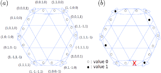
Figure 1.1: A simple example of the KS theorem in action, due to Cabello et al. [14]. Figure (a) lists the vectors (and corresponding rank 1 projectors) associated with the nodes of the hypergraph, with the four nodes in each edge constituting an orthonormal basis. The normalization factors are omitted to avoid clutter, but are presumed, so each vector should be appropriately normalized to a unit vector. The black and white nodes in figure (b) denote value assignments $1$ and $0$ respectively. An attempt at such a value assignment is shown to fail. Indeed, any such attempt will fail.

Figure 1.1 shows such an example: the nodes in Fig. 1.1 denote measurement events in quantum theory, i.e. $18$ rays in a $4$-dimensional Hilbert space, each associated with a corresponding projector associated to a measurement event. The loops in Fig. 1.1 denote measurements, each consisting of four mutually exclusive and jointly exhaustive measurement events. What this means is that the $4$ projectors in each loop correspond to an orthonormal basis in $\mathcal{H}\cong\mathbb{C}^{4}$. Thus, we have $18$ rays carved up into $9$ orthonormal bases of $4$ rays each. The (unnormalized) vectors associated with the rays are labelled in Fig. 1.1(a). The normalization is omitted for clarity in the figure but we are imagining orthonormal bases in this example.

The operational equivalence between measurement events in Fig. 1.1 are implicit in the fact that every projector is shared between two orthonormal bases, each basis representing a context for the projector. The measurement event consists of a specification of the projector along with the orthonormal basis it’s considered to be a part of, and we know that regardless of which orthonormal basis a projector appears in, the probability of occurrence of a measurement event associated with it is the same for any quantum state. This latter fact denotes the operational equivalence of the two measurement events corresponding to the same projector.

Measurement noncontextuality now requires that in an ontological model the physical state of the system $\lambda$ specifies the probabilities of occurrence of measurement events independent of their context, i.e., for operationally equivalent measurement events, the same probabilities are assigned to them by $\lambda$. This condition of measurement noncontextuality on its own can be satisfied for the measurement events depicted in Fig. 1.1. It just translates to being able to assign probabilities to the nodes in Fig. 1.1 in such a way that they add up to $1$ for each loop. However, the Kochen-Specker contradiction arises when an additional requirement, besides measurement noncontextuality, is made: that the probabilities assigned by $\lambda$ be $\{0,1\}$-valued or deterministic. Thus, instead of a measurement noncontextual assignment of probabilities, we now require a measurement noncontextual assignment of $\{0,1\}$ values by $\lambda$ to the measurement events in Fig. 1.1. As depicted in Fig. 1.1(b), any such attempt at a measurement noncontextual value-assignment – a KS-colouring – fails and therefore there cannot exist a $\lambda$ which makes such assignments of values, proving the Kochen-Specker theorem. To see why any such attempt would fail, it suffices to note the following: the fact that there are $9$ bases means that the total number of projectors assigned value $1$ by $\lambda$ should be odd, since measurement in each basis must result in exactly one projector that occurs for a given $\lambda$; but since each projector appears in two bases, each of those assigned value $1$ will appear in two bases, requiring an even number of projectors assigned value $1$, leading to the Kochen-Specker contradiction. Such a proof of the KS theorem is called a KS-uncolourability proof.

The KS theorem therefore forces a choice between abandoning:

1. measurement noncontextuality, or

2. outcome determinism, or

3. both, measurement noncontextuality and outcome determinism.

Traditionally, outcome determinism has been taken for granted in ontological models of quantum theory and the conclusion then to be derived from the Kochen-Specker theorem is measurement contextuality (or, simply, “contextuality” in the Kochen-Specker framework). Alternatively, one may preserve measurement noncontextuality at the expense of outcome determinism and conclude that any ontological model of quantum theory must admit “intrinsic randomness” or outcome indeterminism.

As an argument against the principle of noncontextuality due to Spekkens[6], however, the Kochen-Specker theorem fails: it’s always possible to salvage measurement noncontextuality by abandoning outcome determinism. How then does the Spekkens approach recover or operationalize the Kochen-Specker theorem? This is where preparation noncontextuality enters the picture: using the operational fact that projectors exhibit perfect predictability when measured on the corresponding eigenstate, and the assumption of preparation noncontextuality, it is possible to infer outcome determinism for sharp (projective) measurements, or “ODSM”, in quantum theory. We sketch the argument below, based on Ref. [6].

Theorem 2.

Preparation noncontextuality (PNC) implies outcome determinism for sharp measurements (ODSM) in ontological models of quantum theory.

Proof.

Given a set of rank-1 projectors $M\equiv\{\Pi_{i}\}$ constituting a PVM, i.e. $\Pi_{i}\Pi_{j}=\delta_{ij}\Pi_{i}$ and $\sum_{i}\Pi_{i}=I$, we can write down the corresponding set of pure state density operators $\{\rho_{i}\}$, where $\rho_{i}=\Pi_{i}$ for all $i$. In the ontological model, the measurement events $\Pi_{i}$ are represented by the corresponding response functions $\xi(\Pi_{i}|\lambda)\in[0,1]$ and the preparations $\rho_{i}$ are represented by the corresponding distributions $\mu_{i}(\lambda)\geq 0$, where $\sum_{i}\xi(\Pi_{i}|\lambda)=1$ for all $\lambda\in\Lambda$ and $\sum_{\lambda\in\Lambda}\mu_{i}(\lambda)=1$ for all $i$. We first prove a lemma that will be used later:

Lemma 1.

If two preparations $P$ and $P^{\prime}$ are distinguishable with certainty in a single-shot measurement, then the distributions representing them in the ontological model should be non-overlapping, i.e.

$$\mu(\lambda|P)\mu(\lambda|P^{\prime})=0\quad\forall\lambda\in\Lambda.$$ (1.15)

Proof.

For $P$ and $P^{\prime}$ to be distinguishable with certainty in a single-shot measurement, there must exist a measurement event $E$ in the operational theory such that $p(E|P)=1$ and $p(E|P^{\prime})=0$. The occurrence of $E$ identifies preparation $P$ and its non-occurrence identifies preparation $P^{\prime}$. In the ontological model, this means

$$\sum_{\lambda\in\Lambda}\xi(E|\lambda)\mu(\lambda|P)=1\text{ and }\sum_{\lambda\in\Lambda}\xi(E|\lambda)\mu(\lambda|P^{\prime})=0,$$ (1.16)

so that

$$\xi(E|\lambda)=\begin{cases}1,&\text{ for all }\lambda\in\Lambda_{P}\\ 0,&\text{ for all }\lambda\in\Lambda_{P^{\prime}},\end{cases}$$ (1.17)

where $\Lambda_{P}\equiv\{\lambda\in\Lambda|\mu(\lambda|P)>0\}$ and $\Lambda_{P^{\prime}}\equiv\{\lambda\in\Lambda|\mu(\lambda|P^{\prime})>0\}$. This implies that $\Lambda_{P}\cap\Lambda_{P^{\prime}}=\phi$, because otherwise there exist $\lambda\in\Lambda_{P}\cap\Lambda_{P^{\prime}}$ such that $\xi(E|\lambda)=0$ and $\xi(E|\lambda)=1$, a contradiction. $\Lambda_{P}\cap\Lambda_{P^{\prime}}=\phi$ implies that $\mu(\lambda|P)=0$ for all $\lambda\in\Lambda\backslash\Lambda_{P}\supseteq\Lambda_{P^{\prime}}$ and $\mu(\lambda|P^{\prime})=0$ for all $\lambda\in\Lambda\backslash\Lambda_{P^{\prime}}\supseteq\Lambda_{P}$. We then have

$$\mu(\lambda|P)\mu(\lambda|P^{\prime})=0\quad\forall\lambda\in\Lambda,$$ (1.18)

which is what we set out to prove. ∎

For any two orthogonal rank-1 density operators $\rho_{k}$ and $\rho_{k^{\prime}}$ taken from the set $\{\rho_{i}\}$, it is possible to distinguish them with certainty in a single-shot measurement using either the PVM $\{\Pi_{k},I-\Pi_{k}\}$ or the PVM $\{\Pi_{k^{\prime}},I-\Pi_{k^{\prime}}\}$, since we have

$$\text{Tr}\rho_{k}\rho_{k^{\prime}}=\delta_{k,k^{\prime}}.$$ (1.19)

From Lemma 1, we can therefore conclude that

$$\mu_{k}(\lambda)\mu_{k^{\prime}}(\lambda)=0\quad\forall\lambda\in\Lambda.$$ (1.20)

This implies that $\Lambda_{k}\cap\Lambda_{k^{\prime}}=\phi$ for all $k\neq k^{\prime}$, where $\Lambda_{k}\equiv\{\lambda\in\Lambda|\mu_{k}(\lambda)>0\}$ and $\Lambda_{k^{\prime}}\equiv\{\lambda\in\Lambda|\mu_{k^{\prime}}(\lambda)>0\}$. Given the fact that $\text{Tr}\Pi_{k}\rho_{k^{\prime}}=\delta_{k,k^{\prime}}$, we have in an ontological model

$$\sum_{\lambda}\xi(\Pi_{k}|\lambda)\mu_{k^{\prime}}(\lambda)=\delta_{k,k^{\prime}},$$ (1.21)

so that

$$\xi(\Pi_{k}|\lambda)=\begin{cases}&1\text{ for all }\lambda\in\Lambda_{k},\\ &0\text{ for all }\lambda\in\bigcup_{k^{\prime}\neq k}\Lambda_{k^{\prime}},\end{cases}$$ (1.22)

which is equivalent to

$$\xi(\Pi_{k}|\lambda)\xi(\Pi_{k^{\prime}}|\lambda)=\delta_{k,k^{\prime}}\quad\forall\lambda\in\cup_{i}\Lambda_{i},$$ (1.23)

proving outcome determinism for rank-1 projectors $\{\Pi_{i}\}$ over the ontic support of corresponding quantum states $\{\rho_{i}\}$. In order to prove ODSM in ontological models of quantum theory, we now show that $\cup_{i}\Lambda_{i}=\Lambda$, which establishes outcome determinism over the full set of ontic states $\Lambda$. Here $\Lambda$ is the set of ontic states $\lambda$ which quantum states can sample from, i.e. $\lambda$ such that for every $\lambda\in\Lambda$, there exists a quantum state $\rho$ represented by $\mu_{\rho}(\lambda)>0$ in the ontological model, i.e.

$$\Lambda=\{\lambda|\mu_{\rho}(\lambda)>0\text{ for some }\rho\}.$$ (1.24)

To show $\cup_{i}\Lambda_{i}=\Lambda$, note that

$$\frac{1}{d}\sum_{i}\rho_{i}=\frac{I}{d},$$ (1.25)

an operational equivalence between a uniform mixture of states in $\{\rho_{i}\}$ and the maximally mixed state $\frac{I}{d}$ on a $d$-dimensional Hilbert space. Using the assumption of preparation noncontextuality applied to this operational equivalence, we have

$$\frac{1}{d}\sum_{i}\mu_{i}(\lambda)=\mu_{\frac{I}{d}}(\lambda)\quad\forall\lambda\in\Lambda.$$ (1.26)

This means that every ontic state in the support $\cup_{i}\Lambda_{i}$ also appears in the support $\Lambda_{I/d}$ and conversely, i.e. $\cup_{i}\Lambda_{i}=\Lambda_{I/d}$, where $\Lambda_{I/d}\equiv\{\lambda\in\Lambda|\mu_{I/d}(\lambda)>0\}$.

Now, since every quantum state $\rho$ appears in some convex decomposition of $\frac{I}{d}$, it follows that $\Lambda_{\rho}\subseteq\Lambda_{I/d}$ for all $\rho$, where $\Lambda_{\rho}\equiv\{\lambda\in\Lambda|\mu_{\rho}(\lambda)>0\}$. An example of such a convex decomposition of $I/d$ is the following:

$$\frac{1}{d}\rho+\left(1-\frac{1}{d}\right)\rho^{\prime}=\frac{I}{d},$$ (1.27)

where $\rho^{\prime}=\frac{I-\rho}{d-1}$. Preparation noncontextuality applied to this operational equivalence requires that

$$\frac{1}{d}\mu_{\rho}(\lambda)+\left(1-\frac{1}{d}\right)\mu_{\rho^{\prime}}(\lambda)=\mu_{\frac{I}{d}}(\lambda)\quad\forall\lambda\in\Lambda,$$ (1.28)

so that $\Lambda_{\rho}\subseteq\Lambda_{I/d}$.

Since $\Lambda_{\rho}\subseteq\Lambda_{I/d}$ is true for any quantum state $\rho$, it follows that $\cup_{\rho}\Lambda_{\rho}=\Lambda_{I/d}$. But note that $\cup_{\rho}\Lambda_{\rho}$ is just the set of all ontic states which quantum states can sample from, i.e. $\cup_{\rho}\Lambda_{\rho}=\Lambda$. We therefore have $\Lambda_{I/d}=\Lambda$ and

$$\cup_{i}\Lambda_{i}=\Lambda,$$ (1.29)

implying outcome determinism for rank-1 projectors in quantum theory,

$$\xi(\Pi_{k}|\lambda)\xi(\Pi_{k^{\prime}}|\lambda)=\delta_{k,k^{\prime}}\quad\forall\lambda\in\Lambda,$$ (1.30)

or $\xi(\Pi_{k}|\lambda)\in\{0,1\}$ for all $\lambda\in\Lambda$.

Any sharp measurement or PVM in quantum theory can be obtained by coarse graining rank-1 projectors and since the response functions of rank-1 projectors are deterministic, any coarse-grainings corresponding to elements of a PVM will also be deterministic. This proves that PNC$\Rightarrow$ODSM in ontological models of quantum theory. ∎

We now prove a strengthening of the previous claim that, for ontological models of quantum theory, PNC$\Rightarrow$ODSM. It is, in fact, possible to show that PNC not only implies ODSM, it also implies measurement noncontextuality (MNC), thus recovering the Kochen-Specker notion for noncontextuality for ontological models of quantum theory.

Theorem 3.

Preparation noncontextuality (PNC) implies KS-noncontextuality in ontological models of quantum theory.

Proof.

Consider two PVMs, $\tilde{M}$ and $\tilde{M^{\prime}}$ on a $d$-dimensional Hilbert space. Let $M$ be a coarse-graining of $\tilde{M}$ and $M^{\prime}$ a coarse-graining of $\tilde{M^{\prime}}$, such that both $M$ and $M^{\prime}$ have binary outcomes labelled by $\{0,1\}$ and they are operationally equivalent, i.e. $M\simeq M^{\prime}$ or

$$p(k|M,\rho)=p(k|M^{\prime},\rho)\quad\forall\rho,$$ (1.31)

where $\rho$ is a $d$-dimensional quantum state and $k\in\{0,1\}$. MNC would then require that $\xi(k|M,\lambda)=\xi(k|M^{\prime},\lambda)$ for all $\lambda\in\Lambda$ but we want to derive MNC starting from PNC. Since the operational theory is quantum theory and since $M$ and $M^{\prime}$ are PVMs (because they are coarse-grainings of PVMs), we have that for $M$ there exist two orthogonal preparations $\rho_{0}$ and $\rho_{1}$ such that

$$p(k|M,\rho_{k})=1,\quad k\in\{0,1\}.$$ (1.32)

Since $M\simeq M^{\prime}$, it’s also the case that $p(k|M^{\prime},\rho_{k})=1,k\in\{0,1\}.$ This is easy to see since, in general, $M$ can be represented by PVM elements of the form $[0|M]=\sum_{i=1}^{m}|\alpha_{i}\rangle\langle\alpha_{i}|$ and $[1|M]=\sum_{i=m+1}^{d}|\alpha_{i}\rangle\langle\alpha_{i}|$, where $1\leq m\leq d$ and $\{|\alpha_{i}\rangle\}_{i=1}^{d}$ is an orthonormal basis in the $d$-dimensional Hilbert space so that $\sum_{i=1}^{d}|\alpha_{i}\rangle\langle\alpha_{i}|=I$. Similarly, $M^{\prime}$ can be represented through some other orthonormal basis $\{|\alpha^{\prime}_{i}\rangle\}_{i=1}^{d}$ such that the presumed operational equivalences hold. Note that since $\tilde{M}$ and $\tilde{M^{\prime}}$ are PVMs, they can either be the maximally fine-grained PVMs $\{|\alpha_{i}\rangle\langle\alpha_{i}|\}_{i=1}^{d}$ and $\{|\alpha^{\prime}_{i}\rangle\langle\alpha^{\prime}_{i}|\}_{i=1}^{d}$ respectively, or be obtainable from a coarse-graining of these maximally fine-grained PVMs.

The preparation $\rho_{0}$ then has to lie in the subspace spanned by $\{|\alpha_{i}\rangle\langle\alpha_{i}|\}_{i=1}^{m}$ and the preparation $\rho_{1}$ in the subspace spanned by $\{|\alpha_{i}\rangle\langle\alpha_{i}|\}_{i=m+1}^{d}$ for $p(k|M,\rho_{k})=1$, where $k\in\{0,1\}$, to hold. We will assume $\rho_{0}=\frac{1}{m}\sum_{i=1}^{m}|\alpha_{i}\rangle\langle\alpha_{i}|$ and $\rho_{1}=\frac{1}{d-m}\sum_{i=m+1}^{d}|\alpha_{i}\rangle\langle\alpha_{i}|$. Given the perfect predictability $p(k|M,\rho_{k})=1$ and $p(k|M^{\prime},\rho_{k})=1$ for $k\in\{0,1\}$, it follows that

$$\sum_{\lambda\in\Lambda}\xi(0|M,\lambda)\mu(\lambda|\rho_{0})=1,$$

$$\sum_{\lambda\in\Lambda}\xi(1|M,\lambda)\mu(\lambda|\rho_{1})=1,$$

$$\sum_{\lambda\in\Lambda}\xi(0|M^{\prime},\lambda)\mu(\lambda|\rho_{0})=1,$$

$$\sum_{\lambda\in\Lambda}\xi(1|M^{\prime},\lambda)\mu(\lambda|\rho_{1})=1.$$ (1.33)

Since we have already established PNC$\Rightarrow$ODSM, we have $\xi(k|M,\lambda)$ and $\xi(k|M^{\prime},\lambda)\in\{0,1\}$ for all $\lambda\in\Lambda$. We can now define

$$\Lambda_{M,k}\equiv\{\lambda\in\Lambda|\xi(k|M,\lambda)=1\},$$

$$\Lambda_{M^{\prime},k}\equiv\{\lambda\in\Lambda|\xi(k|M^{\prime},\lambda)=1\}.$$ (1.34)

Since $\xi(1|M,\lambda)=1-\xi(0|M,\lambda)$ and similarly for $M^{\prime}$, we have

$$\Lambda_{M,0}\cup\Lambda_{M,1}=\Lambda,$$ (1.35)

$$\Lambda_{M^{\prime},0}\cup\Lambda_{M^{\prime},1}=\Lambda.$$

Given ODSM, it’s also the case that

$$\Lambda_{M,0}\cap\Lambda_{M,1}=\varnothing,$$

$$\Lambda_{M^{\prime},0}\cap\Lambda_{M^{\prime},1}=\varnothing.$$ (1.36)

It follows that $\xi(k|M,\lambda)=\xi(k|M^{\prime},\lambda)\forall\lambda\in\Lambda$, where $k\in\{0,1\}$, if and only if $\Lambda_{M,0}=\Lambda_{M^{\prime},0}$. We will now show that $\Lambda_{M,0}=\Lambda_{M^{\prime},0}$. From Eq. 1.3.2 we have

$$\sum_{\lambda\in\Lambda_{M,0}}\mu(\lambda|\rho_{0})=1$$

$$\sum_{\lambda\in\Lambda_{M,1}}\mu(\lambda|\rho_{1})=1$$

$$\sum_{\lambda\in\Lambda_{M^{\prime},0}}\mu(\lambda|\rho_{0})=1$$

$$\sum_{\lambda\in\Lambda_{M^{\prime},1}}\mu(\lambda|\rho_{1})=1.$$ (1.37)

From Eqs. 1.35, 1.3.2, and 1.3.2, we have

$$\sum_{\lambda\in\Lambda_{M,0}}\mu(\lambda|\rho_{1})=0,$$

$$\sum_{\lambda\in\Lambda_{M^{\prime},1}}\mu(\lambda|\rho_{0})=0,$$ (1.38)

which implies that

$$\sum_{\lambda\in\Lambda_{M,0}\cap\Lambda_{M^{\prime},1}}\left(\frac{m}{d}\mu(\lambda|\rho_{0})+\left(1-\frac{m}{d}\right)\mu(\lambda|\rho_{1})\right)=0.$$ (1.39)

Now note that

$$\ \frac{m}{d}\rho_{0}+\left(1-\frac{m}{d}\right)\rho_{1}=\frac{I}{d}.$$ (1.40)

Since every quantum state $\rho$ appears in some convex decomposition of the maximally mixed state $\frac{I}{d}$, e.g. $\frac{I}{d}=p\rho+(1-p)\rho^{\prime}$, where $\rho^{\prime}=\frac{I-pd\rho}{d(1-p)}$, the ontic support of $\rho$ is contained in the ontic support of $\frac{I}{d}$. Since $\Lambda$ is just the union of the ontic supports of all quantum states, it is the case that it is equal to the ontic support of $\frac{I}{d}$. It then follows from preparation noncontextuality that

$$\frac{m}{d}\mu(\lambda|\rho_{0})+\left(1-\frac{m}{d}\right)\mu(\lambda|\rho_{1})=\mu(\lambda|I/d)\quad\forall\lambda\in\Lambda,$$ (1.41)

so that the support of $\frac{m}{d}\mu(\lambda|\rho_{0})+\left(1-\frac{m}{d}\right)\mu(\lambda|\rho_{1})$ is $\Lambda$. This in turn means, following Eq. 1.39, that

$$\Lambda_{M,0}\cap\Lambda_{M^{\prime},1}=\varnothing,$$ (1.42)

which implies that

$$\Lambda_{M,0}=\Lambda_{M^{\prime},0}.$$ (1.43)

We therefore have the conclusion we sought: given the operational equivalence $M\simeq M^{\prime}$ and using preparation noncontextuality, we have shown that $\xi(k|M,\lambda)=\xi(k|M^{\prime},\lambda)$ for all $\lambda\in\Lambda$, thus proving measurement noncontextuality (MNC). All in all, we have the conclusion

$$\text{Preparation noncontextuality}\Rightarrow\text{KS-noncontextuality}.$$ (1.44)

∎

This result, then, should convince a skeptic of the relevance of the notion of preparation noncontextuality, which is not as ad hoc as it may appear compared to KS-noncontextuality.

Every proof of the Kochen-Specker theorem is thus also a proof of preparation contextuality but not conversely. Because of the strict implication PNC$\Rightarrow$KS-noncontextuality, preparation noncontextuality is a stronger notion of noncontextuality for ontological models of quantum theory than the traditional notion of KS-noncontextuality. It is indeed possible to rule out preparation noncontextuality without making any appeal to KS-contextuality, as shown in Ref. [6].

1.4 Bell’s theorem

Bell’s theorem provides criteria (Bell inequalities) for ruling out a particular class of ontological models, traditionally called local hidden variable (LHV) models, for composite systems. In particular, the predictions of quantum theory for composite systems rule out LHV ontological models of operational quantum theory. Further, violating Bell inequalities in an experiment rules out an LHV model of Nature itself, rather than merely of the particular operational theory that we currently use to describe Nature. This means that any operational theory offering a putative replacement of quantum theory – our current description of Nature – would necessarily have to fail to admit an LHV model in order to account for experimental violations of Bell inequalities.

The theorem considers a bipartite system prepared by a source according to some distribution $\mu(\lambda|P)$ over the ontic states $\lambda\in\Lambda$, the preparation denoted by $P$. Each part of this bipartite system is sent to one of two parties, Alice and Bob, who are spacelike separated from each other during each run of the experiment. In each run, the experiment involves each party performing a measurement on his/her part of the bipartite system, where the measurement performed is chosen uniformly randomly from two possibilities $\{0,1\}$, followed by recording the two-valued outcome $\{0,1\}$ of this measurement. Alice and Bob implement several runs of the experiment to build up the statistics, $p(a,b|x,y;P)$. Here $x\in\{0,1\}$ denotes the two choices of measurements in Alice’s lab, $y\in\{0,1\}$ denotes the two choices available in Bob’s lab, and $a,b\in\{0,1\}$ denote their respective outcomes for these measurement choices. $p(a,b|x,y;P)$ denotes the joint probability of Alice obtaining outcome $a$ when she performs measurement $x$ on her subsystem and Bob obtaining outcome $b$ when he performs measurement $y$ on his subsystem, where the bipartite system is prepared according to preparation $P$.

Note that since the parties are spacelike separated during the course of their measurements, there should be no signalling between them, i.e. it should not be possible for Alice (Bob) to infer the measurement setting of Bob (Alice) by just looking at her (his) local data $p(a|x;P)$ ($p(b|y;P)$). This no-signalling condition, implied by special relativity, can be expressed as

$$p(a|x;P)=\sum_{b}p(a,b|x,y;P),\quad\forall y\in\{0,1\},\forall a,x\in\{0,1\}$$

$$p(b|y;P)=\sum_{a}p(a,b|x,y;P),\quad\forall x\in\{0,1\},\forall b,y\in\{0,1\}.$$ (1.45)

In the ontological models framework, we have

$$p(a,b|x,y;P) = \sum_{\lambda\in\Lambda}\xi(a,b|x,y;\lambda)\mu(\lambda|P),$$

$$= \sum_{\lambda\in\Lambda}\xi(a|x,y,b;\lambda)\xi(b|x,y;\lambda)\mu(\lambda|P),$$

$$= \sum_{\lambda\in\Lambda}\xi(b|x,y,a;\lambda)\xi(a|x,y;\lambda)\mu(\lambda|P),$$

Bell’s assumption of local causality which defines local hidden variable models then requires the following conditional independences given the ontic state $\lambda$ of the system that is sampled from the source in a particular run of the experiment:

Parameter independence, namely, the independence of one party’s measurement outcome from the other party’s measurement setting,

$$\xi(b|x,y;\lambda) = \xi(b|y;\lambda),$$

$$\xi(a|x,y;\lambda) = \xi(a|x;\lambda),\text{ and}$$ (1.47)

Outcome independence, namely, the independence of one party’s measurement outcome from the other party’s measurement outcome,

$$\xi(a|x,y,b;\lambda) = \xi(a|x,b;\lambda)\text{ (from parameter independence)}=\xi(a|x;\lambda),$$

$$\xi(b|x,y,a;\lambda) = \xi(b|y,a;\lambda)\text{ (from parameter independence)}=\xi(b|y;\lambda).$$ (1.48)

These assumptions are motivated by the fact that spacelike separation should, in an ontological model, result in independence of the statistics in one lab from the statistics in the other lab if the full description of the system, its ontic state $\lambda$ sampled at the source, is specified. The correlations between the two labs arise purely due to ignorance of the exact $\lambda$ that is sampled from one run of the experiment to the other: we presume there exists some distribution $\mu(\lambda|P)$ - characterizing our ignorance of $\lambda$ even when we know the preparation $P$ - according to which $\lambda\in\Lambda$ is sampled.

The conjunction of parameter independence and outcome independence (called local causality) results in

$$p(a,b|x,y;P)=\sum_{\lambda\in\Lambda}\xi(a|x;\lambda)\xi(b|y;\lambda)\mu(\lambda|P),$$ (1.49)

a mathematical condition often called factorizability, since it requires a factorization of the joint probability of measurement outcomes given measurement settings and the ontic state $\lambda$ of the system, i.e. $\xi(a,b|x,y;\lambda)=\xi(a|x;\lambda)\xi(b|y;\lambda)$.

Local causality $\Rightarrow$ no-signalling (but not conversely): It is easy to see that local causality at the ontological level provides a natural account of no-signalling at the operational level, since

$$p(a|x;P) \equiv \sum_{b}p(a,b|x,y;P)$$ (1.50)

$$= \sum_{\lambda\in\Lambda}\xi(a|x;\lambda)\sum_{b}\xi(b|y;\lambda)\mu(\lambda|P)$$

$$= \sum_{\lambda\in\Lambda}\xi(a|x;\lambda)\mu(\lambda|P)$$

is obviously independent of the choice of $y$ on account of factorizability. Similarly,

$$p(b|y;P) \equiv \sum_{a}p(a,b|x,y;P)$$ (1.51)

$$= \sum_{\lambda\in\Lambda}\sum_{a}\xi(a|x;\lambda)\xi(b|y;\lambda)\mu(\lambda|P)$$

$$= \sum_{\lambda\in\Lambda}\xi(b|y;\lambda)\mu(\lambda|P)$$

is independent of $x$. However, notwithstanding the apparent plausibility of the local causality hypothesis as the ontological counterpart of the special relativistic prohibition of faster-than-light propagation of physical influences, it is a matter of experiment whether the hypothesis holds up to scrutiny when tested. These experiments, often called Bell tests, look for violations of constraints (Bell inequalities) on $p(a,b|x,y;P)$ arising from the assumption of local causality. Quantum theory predicts violations of Bell inequalities. When experimentally verified, such violations can be said to be a property of the experiment/Nature without requiring that a quantum model of the experiment/Nature hold.

The CHSH inequality provides the simplest example of a Bell inequality, that is,

$$\sum_{abxy}\frac{1}{4}p(a,b|x,y;P)\delta_{a\oplus b,x.y}\leq\frac{3}{4},$$ (1.52)

where the sum is over those entries $p(a,b|x,y;P)$ for which the input/output correlation $a\oplus b=x.y$ holds. If we denote measurement events by $a_{0}\equiv(a|x=0)$, $a_{1}\equiv(a|x=1)$, $b_{0}\equiv(b|y=0)$, and $b_{1}\equiv(b|y=1)$, then asking that this correlation be satisfied amounts to the following equations:

$$a_{0}\oplus b_{0} = 0,$$ (1.53)

$$a_{0}\oplus b_{1} = 0,$$ (1.54)

$$a_{1}\oplus b_{0} = 0,$$ (1.55)

$$a_{1}\oplus b_{1} = 1.$$ (1.56)

Note that adding up the first three equations gives $a_{1}\oplus b_{1}=0$, contrary to the fourth equation $a_{1}\oplus b_{1}=1$. Thus, at most only three of the four equations can be simultaneously satisfied. The $3/4$ upper bound in the Bell-CHSH inequality arises from this fact.

That this Bell inequality admits a quantum violation can be seen by choosing quantum states and measurements as follows:

Optimal Quantum State

Consider a maximally entangled state of two qubits (each of which is sent to one of the two parties):

$$|\Psi\rangle=\frac{1}{\sqrt{2}}\left(|0\rangle|0\rangle+|1\rangle|1\rangle\right)$$ (1.57)

where we choose the computational basis:

$$|0\rangle=\begin{pmatrix}1\\ 0\end{pmatrix}\text{ and }|1\rangle=\begin{pmatrix}0\\ 1\end{pmatrix}$$

Note that $|\Psi\rangle$ lives in the tensor product Hilbert space $\mathcal{H_{A}}\otimes\mathcal{H_{B}}$, where $\mathcal{H_{A}}$ is the Hilbert space of Alice’s subsystem (qubit) and $\mathcal{H_{B}}$ is the Hilbert space of Bob’s subsystem (qubit). We have omitted the tensor product symbol ‘$\otimes$’ in $|\Psi\rangle$ but the tensor product is presumed. One can now write the corresponding density matrix:

$$\rho=|\Psi\rangle\langle\Psi|=\frac{1}{2}\begin{pmatrix}1&0&0&1\\ 0&0&0&0\\ 0&0&0&0\\ 1&0&0&1\end{pmatrix}$$ (1.58)

Optimal Quantum Measurements

Let us denote the optimal measurements that Alice and Bob perform on their subsystems by $\{A_{0},A_{1}\}$ and $\{B_{0},B_{1}\}$ respectively. They make spin measurements on their qubits:

$$A_{0}=\sigma_{1}=\begin{pmatrix}0&1\\ 1&0\end{pmatrix},\quad A_{1}=\sigma_{3}=\begin{pmatrix}1&0\\ 0&-1\end{pmatrix}$$ (1.59)

$$B_{0}=\frac{\sigma_{1}+\sigma_{3}}{\sqrt{2}}=\frac{1}{\sqrt{2}}\begin{pmatrix}1&1\\ 1&-1\end{pmatrix},\quad B_{1}=\frac{\sigma_{1}-\sigma_{3}}{\sqrt{2}}=\frac{1}{\sqrt{2}}\begin{pmatrix}-1&1\\ 1&1\end{pmatrix}$$ (1.60)

Note that the outcomes for any spin measurement are $\{+1,-1\}$, where we label $+1$ by $`0$’ and $-1$ by $`1$’. The winning probability for the CHSH game given this quantum strategy is:

$$p_{win}^{Q}=\frac{1}{4}\sum_{a,b,x,y\in\{0,1\}}\delta_{a\oplus b,x.y}p(a,b|x,y;\rho),$$ (1.61)

where

$$p(a,b|x,y;\rho)=\text{Tr}(A_{x}^{a}\otimes B_{y}^{b}\rho)=\langle\Psi|A_{x}^{a}\otimes B_{y}^{b}|\Psi\rangle\equiv\langle A_{x}^{a}\otimes B_{y}^{b}\rangle,$$

and

$$A_{x}^{a}=\frac{I+(-1)^{a}A_{x}}{2}$$ (1.62)

$$B_{y}^{b}=\frac{I+(-1)^{b}B_{y}}{2}$$ (1.63)

Clearly,

$$\langle A_{x}^{a}\otimes B_{y}^{b}\rangle=\frac{1}{4}\langle I\otimes I+(-1)^{b}I\otimes B_{y}+(-1)^{a}A_{x}\otimes I+(-1)^{a\oplus b}A_{x}\otimes B_{y}\rangle.$$ (1.64)

We have:

$$p_{win}^{Q} = \frac{1}{4}\sum_{a,b,x,y\in\{0,1\}}\delta_{a\oplus b,x.y}\langle A_{x}^{a}\otimes B_{y}^{b}\rangle$$ (1.65)

$$= \frac{1}{4}\sum_{a,b,x,y\in\{0,1\}}\delta_{a\oplus b,x.y}\frac{1}{4}\langle I\otimes I+(-1)^{b}I\otimes B_{y}+(-1)^{a}A_{x}\otimes I+(-1)^{a\oplus b}A_{x}\otimes B_{y}\rangle$$

$$= \frac{1}{2}\left(1+\frac{\langle A_{0}\otimes B_{0}+A_{0}\otimes B_{1}+A_{1}\otimes B_{0}-A_{1}\otimes B_{1}\rangle}{4}\right)$$

$$= \frac{1}{2}\left(1+\frac{\langle CHSH\rangle}{4}\right),$$

where

$$\langle CHSH\rangle\equiv\langle A_{0}\otimes B_{0}+A_{0}\otimes B_{1}+A_{1}\otimes B_{0}-A_{1}\otimes B_{1}\rangle.$$

Consider spin measurement on Alice’s qubit along $\hat{\alpha}=(\alpha_{1},\alpha_{2},\alpha_{3})$ axis (i.e., measurement of $A^{\alpha}=\vec{\sigma}.\hat{\alpha}$), and measurement on Bob’s qubit along $\hat{\beta}=(\beta_{1},\beta_{2},\beta_{3})$ axis (i.e., measurement of $B^{\beta}=\vec{\sigma}.\hat{\beta}$). Of course, $\vec{\sigma}=(\sigma_{1},\sigma_{2},\sigma_{3})$, where $\sigma_{1}$, $\sigma_{2}$, and $\sigma_{3}$ are the three Pauli matrices:

$$\sigma_{1} = \begin{pmatrix}0&1\\ 1&0\end{pmatrix}$$ (1.66)

$$\sigma_{2} = \begin{pmatrix}0&-i\\ i&0\end{pmatrix}$$ (1.67)

$$\sigma_{3} = \begin{pmatrix}1&0\\ 0&-1\end{pmatrix}$$ (1.68)

corresponding to spin measurements along the $X$, $Y$, and $Z$ axis respectively. Now,

$$\langle A^{\alpha}\otimes B^{\beta}\rangle=\text{Tr}(A^{\alpha}\otimes B^{\beta}\rho)=\alpha_{1}\beta_{1}-\alpha_{2}\beta_{2}+\alpha_{3}\beta_{3}.$$ (1.69)

Denoting any spin measurement $\vec{\sigma}.\hat{\gamma}$ by the corresponding unit vector $(\gamma_{1},\gamma_{2},\gamma_{3})$ along which the measurement is made, we have

$$A_{0}=\sigma_{1}\rightarrow(1,0,0),\quad A_{1}=\sigma_{3}\rightarrow(0,0,1)$$ (1.70)

$$B_{0}=\frac{\sigma_{1}+\sigma_{3}}{\sqrt{2}}\rightarrow\left(\frac{1}{\sqrt{2}},0,\frac{1}{\sqrt{2}}\right),\quad B_{1}=\frac{\sigma_{1}-\sigma_{3}}{\sqrt{2}}=\left(\frac{1}{\sqrt{2}},0,-\frac{1}{\sqrt{2}}\right).$$ (1.71)

Then

$$\langle CHSH\rangle = \langle A_{0}\otimes B_{0}\rangle+\langle A_{0}\otimes B_{1}\rangle+\langle A_{1}\otimes B_{0}\rangle-\langle A_{1}\otimes B_{1}\rangle$$ (1.72)

$$= (1,0,0).(\frac{1}{\sqrt{2}},0,\frac{1}{\sqrt{2}})+(1,0,0).(\frac{1}{\sqrt{2}},0,-\frac{1}{\sqrt{2}})$$

$$+(0,0,1).(\frac{1}{\sqrt{2}},0,\frac{1}{\sqrt{2}})-(0,0,1).(\frac{1}{\sqrt{2}},0,-\frac{1}{\sqrt{2}})$$

$$= 2\sqrt{2},$$

and

$$\therefore p_{win}^{Q}=\frac{1}{2}+\frac{1}{2\sqrt{2}}\approx 0.85,$$ (1.73)

violating the Bell inequality bound of $0.75$.

1.5 Bridging the gap between Bell’s theorem and the Kochen-Specker theorem

Along with its foundational implications, Bell’s theorem[17, 13, 23] has also been the subject of a lot of research activity in quantum information theory. It would not be an exaggeration to say that the seeds for the quantum information age were sown with John Bell’s demonstration of the nontrivial implications of entanglement for the locally causal worldview that quantum theory forces us to abandon. Bell was motivated by the questions Einstein, Podolsky and Rosen raised in their seminal paper[16] questioning the completeness of quantum theory as a description of reality. Today Bell’s theorem underlies many quantum information protocols, ranging from cryptography to randomness generation [2].

On the other hand, the Kochen-Specker theorem has not seen similar explosion of research activity when it comes to its applications to quantum information theory. This is despite the fact, as pointed out often in the recent literature[24, 25, 26], that mathematically speaking, both Bell’s theorem and the Kochen-Specker theorem lead to a marginal problem, i.e. determining whether a given set of variables, carved up into various subsets, can admit a joint probability distribution, given joint probability distributions for the subsets.

The reasons for the relative lack of impact of the Kochen-Specker theorem (as opposed to Bell’s theorem) on the development of quantum information have to do with the idealizations that make the KS theorem less suited to experimental testability and hence applications to quantum information processing. The reasons are foundational since there is a conceptual gap between Bell’s theorem and the Kochen-Specker theorem that is not well-recognized when thinking of both merely mathematically in terms of marginal problems. This gap refers to the following points of contrast between the two theorems, notwithstanding their mathematical similarities:

1. Bell’s theorem is not applicable to a single party. It necessarily requires at least two parties or laboratories for its assumption of local causality to be applied. On the other hand, Kochen-Specker theorem does not need a multipartite scenario for its assumptions to be applicable. One might expect this to count in favour of the Kochen-Specker theorem’s broader applicability but there are significant conceptual hurdles to that.

2. Bell’s theorem is theory-independent: an experimental violation of a Bell inequality rules out local causality irrespective of the particular operational theory that may seek to model the experiment. In particular, one does not need to presume a Hilbert space description of the system (as in quantum theory). On the other hand, the Kochen-Specker theorem is very much a result specific to quantum theory: it presumes that measurement outcomes are represented by projectors on a Hilbert space. Bridging this particular gap between the two theorems requires an operationalization of the Kochen-Specker theorem, a task we take up in Chapter 6.

3. Nonsignalling between the parties during a Bell test is a prerequisite for any observed violations of Bell inequalities to be taken as evidence against local causality. Otherwise the violations can be easily attributed to signalling. Likewise, an operational equivalence between measurement procedures is a prerequisite for any proof of the KS theorem to count as evidence against KS-noncontextuality. However, while nonsignalling is guaranteed by a physical principle independent of quantum theory – namely, the special relativistic prohibition of faster-than-light communication – there is no obvious candidate principle, short of appealing to quantum theory itself, that guarantees operational equivalence between two measurement procedures in a scenario where these measurement procedures may well be carried out on the same system.

4. Bell’s theorem does not require the assumption of outcome determinism while the Kochen-Specker theorem does. We take up this issue in Chapter 5.

5. A fundamental conceptual hurdle to experimentally testing the KS theorem is the existence of Meyer-Kent-Clifton (MKC) type KS-noncontextual models [27] which can simulate the predictions of any set of measurements leading to the Kochen-Specker theorem as long as the measurements are not infinitely precise. In other words, the finite precision of real-world measurements is a loophole that lets MKC-type models reproduce the quantum statistics without giving up on KS-noncontextuality. Such a conceptual hurdle does not apply to Bell’s theorem because it makes no commitment, unlike the KS theorem, regarding the representation of measurements. In the Spekkens’ approach to noncontextuality, the MKC criticism is circumvented by avoiding any use of Hilbert spaces at all – properties of which are crucial to the MKC criticism – akin to discussions of local causality. What remains to be confronted in the Spekkens’ approach is the fact that exact operational equivalences between experimental procedures are an idealization never realized in practice. We take up this issue in the final section of Chapter 6.

1.6 Overview of the thesis

Following this introductory chapter, we will take up the issues highlighted in the last section in the rest of the thesis. In Chapters 2 and 3, we will take the first steps beyond the Kochen-Specker theorem by considering nonprojective quantum measurements and their contextuality. Chapter 4 will show the realizability of arbitrary joint measurability structures when nonprojective measurements are allowed. In Chapter 5, we will show how the assumption of outcome determinism is not as innocuous in the KS theorem as it is in Bell’s theorem (where it’s unnecessary). Chapters 6 and 7 will pursue a full-fledged operationalization of the Kochen-Specker theorem that does not presume quantum theory. Chapter 8 will conclude with some final remarks on the research directions initiated in this thesis and some speculations on what’s next.

Chapter 2 A first look at Specker’s scenario

It is no exaggeration to say that this theorem – the Kochen-Specker theorem – is one of the deepest facts about the foundations of quantum theory. The story of how Specker first started down the road which led to this result is quite wonderful. It shows that even in an era where “shut up and calculate” is the mantra of many researchers, deep philosophical questions can still lead to great advances in our understanding of the world. It is a story that will warm the heart of anyone who believes that physics should be pursued in a romantic style…[Specker] was led to the critical question: could God know what outcome would have occurred had a different quantum measurement been done to the one that was actually done, without getting into contradiction? The answer, he found, was that He could not.

R.W. Spekkens, Ernst Paul Specker (1920-2011), Mind & Matter Vol. 9(2), pp. 121-128.

In 1960, Ernst Specker wrote an article on the logic of quantum theory [28]. In it he uses a parable to illustrate the non-Boolean nature of quantum logic. Liang, Spekkens, and Wiseman [29] studied a modern rendition of Specker’s parable with three unsharp (nonprojective) quantum measurements which are pairwise jointly measurable but not triplewise so. In this chapter, we consider the question of whether such measurements exhibit contextuality, something which was conjectured not to be the case in Ref. [29].

This chapter is based on work reported in Ref. [30].

2.1 Introduction

Quantum theory does not admit Bell-local or KS-noncontextual ontological models. This is manifest in the Bell-nonlocality [16, 17] and KS-contextuality [10] of the theory. Both these features arise—at a mathematical level—from the lack of a global joint probability distribution over measurement outcomes that can reproduce the measurement statistics predicted by quantum theory. Traditionally, KS-contextuality has been shown with respect to projective measurements for Hilbert spaces of dimension three or greater [10, 32, 31, 33, 14, 34, 36, 35, 37].

For projective measurements, KS-noncontextuality is the assumption that in an ontological model of quantum theory the outcome of a measurement $A$ is independent of whether it is performed together with a measurement $B$, where $[A,B]=0$, or with measurement $C$, where $[A,C]=0$ and $B$ and $C$ are not compatible, i.e. $[B,C]\neq 0$. $B$ and $C$ provide contexts for measurement of $A$. A qubit cannot yield a proof of KS-contextuality because, having only a maximum of two mutually orthogonal rank 1 projectors, it does not allow projective measurements $A,B,C$ such that $[A,B]=0,[A,C]=0$, and $[B,C]\neq 0$. The existence of a triple of such projective measurements is necessary for any proof of KS-contextuality. While a state-independent proof of KS-contextuality holds for any state preparation, a state-dependent proof requires a special choice of the prepared state. The minimal state-independent proof of KS-contextuality requires a qutrit and $13$ projectors [37, 38]. The minimal state-dependent proof [35, 36], first given by Klyachko et al., requires a qutrit and five projectors (Fig. 2.1). Thus a qutrit is the simplest quantum system that allows a proof of KS-contextuality, both state-independent and state-dependent.

However, generalizations of KS-noncontextuality for a qubit have been considered earlier [39, 40, 41] in a manner that is conceptually distinct from the approach we adopt here. These generalizations typically apply the assumption of outcome determinism to unsharp (nonprojective) measurements. Such an application of this assumption cannot be justified from noncontextuality alone, as amply demonstrated in Ref. [42]. Our approach builds upon the work of Spekkens [6] and Liang et. al. [29], and we consider generalized-noncontextuality proposed by Spekkens [6] as the appropriate notion of noncontextuality for unsharp qubit measurements. This notion of noncontextuality allows one to consider outcome-indeterministic response functions for unsharp measurements in the ontological model, indeed it requires them[42], while any naive application of KS-noncontextuality to POVMs would insist on outcome-deterministic response functions. Since we have already introduced the definitions of noncontextuality in Chapter 1, we will not repeat them here.

We define a compatibility scenario as a collection of subsets, called ‘compatibility contexts’, of the set of all measurements. A compatibility context refers to measurements that can be jointly implemented.

Figure 2.1: The KCBS [35] compatibility scenario. The vertices represent the measurements and edges represent compatibility contexts (of jointly measurable observables).

Conceptually, the simplest possible compatibility scenario capable of exhibiting KS-contextuality, first considered by Specker [28] (Fig. 4.1), requires three two-valued measurements, $\{M_{1},M_{2},M_{3}\}$, to allow for three non-trivial compatibility contexts: $\{\{M_{1},M_{2}\},\{M_{1},M_{3}\},\{M_{2},M_{3}\}\}$. Any other choice of contexts will be trivially KS-noncontextual, e.g., $\{\{M_{1},M_{2}\},\{M_{1},M_{3}\}\}$ is KS-noncontextual because the joint probability distribution

$$p(M_{1},M_{2},M_{3})\equiv p(M_{1},M_{2})p(M_{1},M_{3})/p(M_{1})$$

reproduces the marginal statistics for $\{M_{1},M_{2}\}$ and $\{M_{1},M_{3}\}$. In Specker’s scenario, measurement statistics that always shows perfect anticorrelation between any two measurements sharing a context is necessarily KS-contextual. On assigning outcomes $\{+1,-1\}$ KS-noncontextually to the three measurements $\{M_{1},M_{2},M_{3}\}$, it becomes obvious that the maximum number of anticorrelated contexts possible in a single assignment is two, e.g., for the assignment $\{M_{1}\rightarrow+1,M_{2}\rightarrow-1,M_{3}\rightarrow+1\}$, $\{M_{1},M_{2}\}$ and $\{M_{2},M_{3}\}$ are anticorrelated but $\{M_{1},M_{3}\}$ is not. This puts an upper bound of $\frac{2}{3}$ on the probability of anticorrelation when a context is chosen uniformly at random. Specker’s scenario precludes projective measurements because a set of three pairwise commuting projective measurements is trivially jointly measurable and cannot show any contextuality. One may surmise that it represents a kind of contextuality that is not seen in quantum theory. However, as Liang et al. showed [29], Specker’s scenario can be realized using noisy spin-1/2 observables. They showed that if one does not assume outcome-determinism for unsharp measurements and models them stochastically but noncontextually, then this noncontextual model for noisy spin-1/2 observables will obey a bound of $1-\frac{\eta}{3}$, where $\eta\in[0,1]$ is the sharpness associated with each observable. Formally,

$$R_{3}\equiv\frac{1}{3}\sum_{(ij)\in\{(12),(23),(13)\}}\textrm{Pr}(X_{i}\neq X_{j}|G_{ij})\leq 1-\frac{\eta}{3},$$ (2.1)

where $\textrm{Pr}(X_{i}\neq X_{j}|G_{ij})$ is the probability of anticorrelation between the outcomes $X_{i},X_{j}\in\{+1,-1\}$ of measurements $M_{i}$ and $M_{j}$, respectively. $G_{ij}$ denotes the joint implementation of $M_{i}$ and $M_{j}$. We will refer to this noncontextuality inequality as the LSW (Liang-Spekkens-Wiseman) inequality. Note that the LSW inequality is not a KS-noncontextuality inequality, for which the bound would be $\frac{2}{3}$. A violation of the LSW inequality will rule out Spekkens’ generalized notion of noncontextuality and, by implication, KS-noncontextuality. After giving examples of orthogonal and trine spin-axes that did not seem to show a violation of this inequality, Liang et al. left open the question of whether such a violation exists [29]. They conjectured that all such triples of POVMs will admit a noncontextual model [6], i.e. the LSW inequality will not be violated. We settle this conjecture by showing that, contrary to their expectation[29], the LSW inequality does admit a quantum violation.

Figure 2.2: Specker’s scenario.

2.2 The LSW inequality

The three POVMs considered, $M_{k}=\{E^{k}_{+},E^{k}_{-}\}$, $k\in\{1,2,3\}$, are noisy spin-$\frac{1}{2}$ observables of the form

$$E^{k}_{\pm}\equiv\frac{1}{2}I\pm\frac{\eta}{2}\vec{\sigma}.\hat{n}_{k},\quad 0\leq\eta\leq 1.$$ (2.2)

That is,

$$E^{k}_{\pm}=\frac{1-\eta}{2}I+\eta\Pi^{k}_{\pm},$$ (2.3)

where $\Pi^{k}_{\pm}=\frac{1}{2}(I\pm\vec{\sigma}.\hat{n}_{k})$ are the corresponding projectors. So $E^{k}_{\pm}$ are noisy versions of the projectors $\Pi^{k}_{\pm}$, and the observable $\{E^{k}_{+},E^{k}_{-}\}$ is therefore a noisy (or unsharp) version of the projective measurement $P_{k}=\{\Pi^{k}_{+},\Pi^{k}_{-}\}$ (for $k\in\{1,2,3\}$):

$$\{E^{k}_{+},E^{k}_{-}\}=\eta\{\Pi^{k}_{+},\Pi^{k}_{-}\}+(1-\eta)\{I/2,I/2\}.$$

The LSW inequality concerns the following quantity:

$$R_{3}\equiv\frac{1}{3}\sum_{(ij)\in\{(12),(23),(13)\}}p(X_{i}\neq X_{j}|G_{ij})$$ (2.4)

where $X_{i},X_{j}\in\{+1,-1\}$ label measurement outcomes for $M_{i}$ and $M_{j}$, respectively. The joint measurement POVM for the context $\{M_{i},M_{j}\}$ is denoted by $G_{ij}\equiv\{G_{++}^{ij},G_{+-}^{ij},G_{-+}^{ij},G_{--}^{ij}\}$. $G^{ij}_{X_{i},X_{j}}$ is the joint measurement effect corresponding to the effects $E^{i}_{X_{i}}$ and $E^{j}_{X_{j}}$, i.e.

$$\sum_{X_{j}}G^{ij}_{X_{i},X_{j}}=E^{i}_{X_{i}}\text{ and }\sum_{X_{i}}G^{ij}_{X_{i},X_{j}}=E^{j}_{X_{j}}.$$

$R_{3}$ is the average probability of anticorrelation when one of the three contexts is chosen uniformly at random.

Under the assumption of noncontextuality for these noisy spin-1/2 observables, the following bound on $R_{3}$ holds (cf. [29], Section 7.3):

$$R_{3}\leq 1-\frac{\eta}{3}$$ (2.5)

The question is: Does there exist a triple of noisy spin-1/2 observables that will violate this inequality, perhaps for some specific state-preparation?

2.3 Joint measurability constraints

Testing the LSW inequality for a quantum mechanical violation requires a special kind of joint measurability (or compatibility), denoted by compatibility contexts $\{\{M_{1},M_{2}\}$, $\{M_{2},M_{3}\}$, $\{M_{1},M_{3}\}\}$, i.e. pairwise joint measurability but no triplewise joint measurability. One can achieve this joint measurability criterion by adding noise to projective measurements along three different axes. For a given choice of measurement directions $\{\hat{n}_{1},\hat{n}_{2},\hat{n}_{3}\}$ in Eq. (2.2), denoting $\hat{n}_{i}.\hat{n}_{j}\equiv\cos\theta_{ij}$, a sufficient condition for this kind of joint measurability is

$$\eta_{l}<\eta\leq\eta_{u}$$ (2.6)

where

$$\eta_{l}=\frac{1}{3}\max_{X_{1},X_{2},X_{3}\in\{\pm 1\}}\left\{\sqrt{3+2\sum_{k,l\in\{1,2,3\},k<l}X_{k}X_{l}\cos\theta_{kl}}\right\}$$ (2.7)

and

$$\eta_{u}=\min_{(ij)\in\{(12),(23),(13)\}}\left\{\frac{1}{\sqrt{1+|\sin\theta_{ij}|}}\right\}$$ (2.8)

We note that this condition is necessary and sufficient for the special case of trine ($\hat{n}_{i}.\hat{n}_{j}=-1/2$) and orthogonal ($\hat{n}_{i}.\hat{n}_{j}=0$) spin axes. These conditions are obtained as special cases of the more general joint measurability conditions we now prove, based on Refs. [29] and [43].

Bounds on $\eta$ from joint measurability: In Appendix F of Ref. [29], Theorem 13, the authors obtain necessary and sufficient conditions for joint measurability of noisy spin-1/2 observables. We note that the claimed necessary condition in the aforementioned theorem is incorrect, while the sufficient condition holds. Hence we prove a necessary condition for joint measurability that we use for triplewise joint measurability, thereby correcting the argument for necessity made by Liang et al.:

Theorem 4.

Given a set of qubit POVMs, $\{\{E^{k}_{X_{k}}:X_{k}\in\{+1,-1\}\}|k\in\{1\dots N\}\}$, of the form

$$E^{k}_{X_{k}}=\frac{1}{2}I+\frac{1}{2}\vec{\sigma}.X_{k}\eta\hat{n}_{k},$$ (2.9)

and defining $2^{N}$ 3-vectors

$$\vec{m}_{X_{1}\dots X_{N}}\equiv\sum_{k=1}^{N}X_{k}\hat{n}_{k},$$ (2.10)

a necessary condition for all the POVMs to be jointly measurable is that

$$\eta\leq\frac{1}{N}\max_{X_{1}\dots X_{N}}\{|\vec{m}_{X_{1}\dots X_{N}}|\},$$ (2.11)

and a sufficient condition is that

$$\eta\leq\frac{2^{N}}{\sum_{X_{1}\dots X_{N}}|\vec{m}_{X_{1}\dots X_{N}}|}.$$ (2.12)

Proof. We will only prove the necessary condition and refer the reader to Ref.[29], Appendix F, for proof of the sufficient condition. Note that $\eta=\text{Tr}\left[(\vec{\sigma}.X_{k}\hat{n}_{k})E^{k}_{X_{k}}\right]$. Since this holds $\forall X_{k},k$, we have

$$\eta=\frac{1}{2N}\sum_{k=1}^{N}\sum_{X_{k}}\text{Tr}\left[(\vec{\sigma}.X_{k}\hat{n}_{k})E^{k}_{X_{k}}\right]$$ (2.13)

If all the POVMs are jointly measurable, then we must necessarily have a joint POVM $\{E_{X_{1}\dots X_{N}}\}$ such that

$$E^{k}_{X_{k}}=\sum_{X_{1}\dots X_{k-1},X_{k+1}\dots X_{N}}E_{X_{1}\dots X_{N}}.$$ (2.14)

Then,

$$\eta=\frac{1}{2N}\sum_{X_{1}\dots X_{N}}\text{Tr}\left[\left(\vec{\sigma}.\sum_{k=1}^{N}X_{k}\hat{n}_{k}\right)E_{X_{1}\dots X_{N}}\right],$$ (2.15)

and using $\hat{m}_{X_{1}\dots X_{N}}\equiv\vec{m}_{X_{1}\dots X_{N}}/|\vec{m}_{X_{1}\dots X_{N}}|$, we have

$$\eta=\frac{1}{2N}\sum_{X_{1}\dots X_{N}}|\vec{m}_{X_{1}\dots X_{N}}|\text{Tr}\left[\left(\vec{\sigma}.\hat{m}_{X_{1}\dots X_{N}}\right)E_{X_{1}\dots X_{N}}\right].$$ (2.16)

Further,

$$\text{Tr}\left[\left(\vec{\sigma}.\hat{m}_{X_{1}\dots X_{N}}\right)E_{X_{1}\dots X_{N}}\right]\leq\text{Tr}\left[E_{X_{1}\dots X_{N}}\right],$$ (2.17)

which yields the inequality

$$\eta\leq\frac{1}{2N}\sum_{X_{1}\dots X_{N}}|\vec{m}_{X_{1}\dots X_{N}}|\text{Tr}\left[E_{X_{1}\dots X_{N}}\right].$$ (2.18)

Now, $\sum_{X_{1}\dots X_{N}}E_{X_{1}\dots X_{N}}=I$, and therefore,

$$\sum_{X_{1}\dots X_{N}}\frac{1}{2}\text{Tr}\left[E_{X_{1}\dots X_{N}}\right]=1.$$ (2.19)

Also, $0\leq\frac{1}{2}\text{Tr}\left[E_{X_{1}\dots X_{N}}\right]\leq 1$, so we have, by convexity of the set $\left\{\frac{1}{2}\text{Tr}\left[E_{X_{1}\dots X_{N}}\right]\right\}_{X_{1}\dots X_{N}}$,

$$\eta\leq\frac{1}{N}\max_{X_{1}\dots X_{N}}\left\{|\vec{m}_{X_{1}\dots X_{N}}|\right\},$$ (2.20)

which is a necessary condition for joint measurability. For $N=3$ we obtain the necessary condition for triplewise joint measurability which we use for computing $\eta_{l}$. The necessary and sufficient condition for pairwise joint measurability is given by

$$1+\eta^{4}(\hat{n}_{i}.\hat{n}_{j})^{2}-2\eta^{2}\geq 0,\quad\forall(ij)\in\{(12),(13),(23)\}.$$ (2.21)

This is obtained as a special case, for the present problem, of the more general necessary and sufficient condition for joint measurability of pairs of unsharp qubit observables obtained in Ref. [43]. Using $\hat{n}_{i}.\hat{n}_{j}=\cos\theta_{ij}$, this inequality becomes

$$\left(\eta^{2}-\frac{1}{1-|\sin\theta_{ij}|}\right)\left(\eta^{2}-\frac{1}{1+|\sin\theta_{ij}|}\right)\geq 0.$$ (2.22)

Since $0\leq\eta\leq 1$, the necessary and sufficient condition for pairwise joint measurability becomes

$$\eta\leq\min_{(ij)\in\{(12),(23),(13)\}}\left\{\frac{1}{\sqrt{1+|\sin\theta_{ij}|}}\right\},$$ (2.23)

which is used to compute $\eta_{u}$.

Orthogonal spin axes: $\hat{n}_{i}.\hat{n}_{j}=0$ for all $(ij)\in\{(12),(13),(23)\}$. The necessary and sufficient joint measurability condition is

$$\frac{1}{\sqrt{3}}<\eta\leq\frac{1}{\sqrt{2}}.$$ (2.24)

Trine spin axes: $\hat{n}_{i}.\hat{n}_{j}=-1/2$ for all $(ij)\in\{(12),(13),(23)\}$. The necessary and sufficient joint measurability condition is

$$\frac{2}{3}<\eta\leq\sqrt{3}-1.$$ (2.25)

Joint measurement effects: We construct the joint measurement POVM,

$$G_{ij}=\{G^{ij}_{++},G^{ij}_{+-},G^{ij}_{-+},G^{ij}_{--}\},$$

such that the given POVMs, $M_{i}=\{E^{i}_{+},E^{i}_{-}\}$ and $M_{j}=\{E^{j}_{+},E^{j}_{-}\}$, are recovered as marginals, i.e., $\sum_{X_{j}}G^{ij}_{X_{i},X_{j}}=E^{i}_{X_{i}}$, $\sum_{X_{i}}G^{ij}_{X_{i},X_{j}}=E^{j}_{X_{j}}$, $0\leq G^{ij}_{X_{i},X_{j}}\leq I$, and $\sum_{X_{i},X_{j}}G^{ij}_{X_{i},X_{j}}=I$, where $X_{i},X_{j}\in\{+1,-1\}$. The joint measurement POVM has the following general form:

$$G^{ij}_{++} = \frac{1}{2}\left[\frac{\alpha_{ij}}{2}I+\vec{\sigma}.\frac{1}{2}\left(\eta(\hat{n}_{i}+\hat{n}_{j})-\vec{a}_{ij}\right)\right],$$ (2.26)

$$G^{ij}_{+-} = \frac{1}{2}\left[\left(1-\frac{\alpha_{ij}}{2}\right)I+\vec{\sigma}.\frac{1}{2}\left(\eta(\hat{n}_{i}-\hat{n}_{j})+\vec{a}_{ij}\right)\right],$$ (2.27)

$$G^{ij}_{-+} = \frac{1}{2}\left[\left(1-\frac{\alpha_{ij}}{2}\right)I+\vec{\sigma}.\frac{1}{2}\left(\eta(-\hat{n}_{i}+\hat{n}_{j})+\vec{a}_{ij}\right)\right],$$ (2.28)

$$G^{ij}_{--} = \frac{1}{2}\left[\frac{\alpha_{ij}}{2}I+\vec{\sigma}.\frac{1}{2}\left(\eta(-\hat{n}_{i}-\hat{n}_{j})-\vec{a}_{ij}\right)\right],$$ (2.29)

where $I$ is the $2\times 2$ identity matrix, $\vec{\sigma}=(\sigma_{x},\sigma_{y},\sigma_{z})$ are the $2\times 2$ Pauli matrices, $\alpha_{ij}\in\mathbb{R}$, and $\vec{a}_{ij}\in\mathbb{R}^{3}$. The necessary and sufficient conditions for these to be valid qubit effects, $0\leq G^{ij}_{X_{i},X_{j}}\leq I$, $\forall X_{i},X_{j}\in\{+1,-1\}$, are equivalent to the following inequalities [44],

$$\sqrt{2\eta^{2}(1+\hat{n}_{i}.\hat{n}_{j})+|\vec{a}_{ij}|^{2}+2\eta|(\hat{n}_{i}+\hat{n}_{j}).\vec{a}_{ij}|}\leq\alpha_{ij}$$ (2.30)

$$\alpha_{ij}\leq 2-\sqrt{2\eta^{2}(1-\hat{n}_{i}.\hat{n}_{j})+|\vec{a}_{ij}|^{2}+2\eta|(\hat{n}_{i}-\hat{n}_{j}).\vec{a}_{ij}|},$$ (2.31)

where $\eta_{l}<\eta\leq\eta_{u}$. The joint measurement effects corresponding to anticorrelation sum to

$$G^{ij}_{+-}+G^{ij}_{-+}=\left(1-\frac{\alpha_{ij}}{2}\right)I+\frac{1}{2}\vec{\sigma}.\vec{a}_{ij}.$$ (2.32)

We now come to the construction of the joint measurement POVM and derivation of the necessary and sufficient condition for its validity, Eqs. (2.30)-(2.31).

Constructing the joint measurement: The joint measurement POVM $G_{ij}$ for $\{M_{i},M_{j}\}$ should satisfy the marginal condition:

$$G^{ij}_{++}+G^{ij}_{+-}=E^{i}_{+},\quad G^{ij}_{-+}+G^{ij}_{--}=E^{i}_{-},$$ (2.33)

$$G^{ij}_{++}+G^{ij}_{-+}=E^{j}_{+},\quad G^{ij}_{+-}+G^{ij}_{--}=E^{j}_{-}.$$ (2.34)

Also, the joint measurement should consist of valid effects:

$$0\leq G^{ij}_{++},G^{ij}_{+-},G^{ij}_{-+},G^{ij}_{--}\leq I,$$ (2.35)

where $I$ is the $2\times 2$ identity matrix. The general form of the joint measurement effects is:

$$G^{ij}_{++} = \frac{1}{2}\left[\frac{\alpha_{ij}}{2}I+\vec{\sigma}.\vec{a}^{ij}_{++}\right],$$ (2.36)

$$G^{ij}_{+-} = \frac{1}{2}\left[\left(1-\frac{\alpha_{ij}}{2}\right)I+\vec{\sigma}.\vec{a}^{ij}_{+-}\right],$$ (2.37)

$$G^{ij}_{-+} = \frac{1}{2}\left[\left(1-\frac{\alpha_{ij}}{2}\right)I+\vec{\sigma}.\vec{a}^{ij}_{-+}\right],$$ (2.38)

$$G^{ij}_{--} = \frac{1}{2}\left[\frac{\alpha_{ij}}{2}I+\vec{\sigma}.\vec{a}^{ij}_{--}\right],$$ (2.39)

where each effect is parameterized by four real numbers. From the marginal condition, Eqs. (2.33-2.34), it follows that:

$$\vec{a}^{ij}_{++}+\vec{a}^{ij}_{+-}=\eta\hat{n}_{i},\quad\vec{a}^{ij}_{-+}+\vec{a}^{ij}_{--}=-\eta\hat{n}_{i},$$ (2.40)

$$\vec{a}^{ij}_{-+}+\vec{a}^{ij}_{++}=\eta\hat{n}_{j},\quad\vec{a}^{ij}_{--}+\vec{a}^{ij}_{+-}=-\eta\hat{n}_{j}.$$ (2.41)

These can be rewritten as:

$$2\vec{a}^{ij}_{++}+\vec{a}^{ij}_{+-}+\vec{a}^{ij}_{-+} = \eta(\hat{n}_{i}+\hat{n}_{j}),$$ (2.42)

$$2\vec{a}^{ij}_{+-}+\vec{a}^{ij}_{++}+\vec{a}^{ij}_{--} = \eta(\hat{n}_{i}-\hat{n}_{j}),$$ (2.43)

$$2\vec{a}^{ij}_{-+}+\vec{a}^{ij}_{++}+\vec{a}^{ij}_{--} = \eta(-\hat{n}_{i}+\hat{n}_{j}),$$ (2.44)

$$2\vec{a}^{ij}_{--}+\vec{a}^{ij}_{+-}+\vec{a}^{ij}_{-+} = \eta(-\hat{n}_{i}-\hat{n}_{j}).$$ (2.45)

From Eqs. (2.40-2.41) it follows that:

$$(\vec{a}^{ij}_{++}+\vec{a}^{ij}_{--})+(\vec{a}^{ij}_{-+}+\vec{a}^{ij}_{+-})=0.$$

So one can define:

$$\vec{a}_{ij}\equiv\vec{a}^{ij}_{+-}+\vec{a}^{ij}_{-+}\Rightarrow\vec{a}^{ij}_{++}+\vec{a}^{ij}_{--}=-\vec{a}_{ij}.$$

Now, from Eqs. (2.42)-(2.45) the following are obvious:

$$\vec{a}^{ij}_{++} = \frac{1}{2}\left[\eta\left(\hat{n}_{i}+\hat{n}_{j}\right)-\vec{a}_{ij}\right],$$ (2.46)

$$\vec{a}^{ij}_{+-} = \frac{1}{2}\left[\eta\left(\hat{n}_{i}-\hat{n}_{j}\right)+\vec{a}_{ij}\right],$$ (2.47)

$$\vec{a}^{ij}_{-+} = \frac{1}{2}\left[\eta\left(-\hat{n}_{i}+\hat{n}_{j}\right)+\vec{a}_{ij}\right],$$ (2.48)

$$\vec{a}^{ij}_{--} = \frac{1}{2}\left[\eta\left(-\hat{n}_{i}-\hat{n}_{j}\right)-\vec{a}_{ij}\right].$$ (2.49)

This gives the general form of the joint measurement POVMs. For qubit effects, $G^{ij}_{X_{i}X_{j}}$, where $X_{i},X_{j}\in\{+1,-1\}$, the valid effect condition, Eq. (2.35), is equivalent to the following [44]:

$$|\vec{a}^{ij}_{++}| \leq \frac{\alpha_{ij}}{2}\leq 2-|\vec{a}^{ij}_{++}|,$$ (2.50)

$$|\vec{a}^{ij}_{+-}| \leq 1-\frac{\alpha_{ij}}{2}\leq 2-|\vec{a}^{ij}_{+-}|,$$ (2.51)

$$|\vec{a}^{ij}_{-+}| \leq 1-\frac{\alpha_{ij}}{2}\leq 2-|\vec{a}^{ij}_{-+}|,$$ (2.52)

$$|\vec{a}^{ij}_{--}| \leq \frac{\alpha_{ij}}{2}\leq 2-|\vec{a}^{ij}_{--}|.$$ (2.53)

These inequalities can be combined and rewritten as:

$$2\max\left\{|\vec{a}^{ij}_{++}|,|\vec{a}^{ij}_{--}|\right\}\leq\alpha_{ij}\leq 2-2\max\left\{|\vec{a}^{ij}_{+-}|,|\vec{a}^{ij}_{-+}|\right\},$$ (2.54)

where

$$\max\left\{|\vec{a}^{ij}_{++}|,|\vec{a}^{ij}_{--}|\right\}$$

$$=\sqrt{\frac{\eta^{2}}{2}(1+\hat{n}_{i}.\hat{n}_{j})+\frac{|\vec{a}_{ij}|^{2}}{4}+\frac{\eta}{2}|(\hat{n}_{i}+\hat{n}_{j}).\vec{a}_{ij}|}$$

and

$$\max\left\{|\vec{a}^{ij}_{+-}|,|\vec{a}^{ij}_{-+}|\right\}$$

$$=\sqrt{\frac{\eta^{2}}{2}(1-\hat{n}_{i}.\hat{n}_{j})+\frac{|\vec{a}_{ij}|^{2}}{4}+\frac{\eta}{2}|(\hat{n}_{i}-\hat{n}_{j}).\vec{a}_{ij}|}.$$

This is the condition for a valid joint measurement used in inequalities of Eqs. (2.30-2.31).

2.4 No state-independent violation of LSW inequality

We will now show that no state-independent violation of the LSW inequality with qubit POVMs is possible.

Theorem 5.

There exists no state-independent violation of the LSW inequality $R_{3}\leq 1-\frac{\eta}{3}$ using a triple of qubit POVMs, $M_{k}\equiv\{E^{k}_{\pm}\},k\in\{1,2,3\}$, that are pairwise jointly measurable (but not necessarily triplewise jointly measurable).

Proof.

In quantum theory, the probability $R^{Q}_{3}$ for anticorrelation of measurement outcomes for pairwise joint measurements of $M_{k}\equiv\{E^{k}_{+},E^{k}_{-}\}$ (where $k\in\{1,2,3\}$) has the following form for a qubit state $\rho$:

$$R^{Q}_{3}\equiv\frac{1}{3}\sum_{(ij)\in\{(12),(23),(13)\}}\textrm{Tr}\left(\rho\left(G^{ij}_{+-}+G^{ij}_{-+}\right)\right),$$ (2.55)

The condition for violation of noncontextual inequality, Eq. (2.5), is $R_{3}^{Q}>1-\frac{\eta}{3}$. Using Eq. (2.32), this reduces to

$$\textrm{Tr}\left(\rho\sum_{(ij)}(\alpha_{ij}I-\vec{\sigma}.\vec{a}_{ij})\right)<2\eta$$ (2.56)

Using the standard $2\times 2$ Pauli matrices and $\rho$ parameterized by $0\leq q\leq 1$ and $\hat{n}=(\sin\theta\cos\phi,\sin\theta\sin\phi,\cos\theta)$:

$$\rho = q|\psi\rangle\langle\psi|+(1-q)(I-|\psi\rangle\langle\psi|),$$ (2.57)

$$|\psi\rangle = \left(\begin{array}[]{c}\cos\frac{\theta}{2}\\ e^{i\phi}\sin\frac{\theta}{2}\end{array}\right)=\cos\frac{\theta}{2}|0\rangle+e^{i\phi}\sin\frac{\theta}{2}|1\rangle,$$ (2.60)

the condition for violation becomes

$$\sum_{(ij)}\alpha_{ij}+\lambda_{\rho}<2\eta,$$ (2.61)

where

$$\lambda_{\rho}\equiv(1-2q)\vec{a}.\hat{n}\in\left[-|\vec{a}|,|\vec{a}|\right]$$ (2.62)

denotes the state-dependent term in the condition and $\vec{a}=(a_{x},a_{y},a_{z})$ is given by

$$a_{x}=\sum_{(ij)}(\vec{a}_{ij})_{x},\quad a_{y}=\sum_{(ij)}(\vec{a}_{ij})_{y},\quad a_{z}=\sum_{(ij)}(\vec{a}_{ij})_{z}.$$ (2.63)

For a state-independent violation, either the state-dependent term in Eq. (2.61), $\lambda_{\rho}$, must vanish for all qubit states $\rho$, or $\sum_{(ij)}\alpha_{ij}+\max_{\rho}\lambda_{\rho}<2\eta$ should hold. The first case, $\lambda_{\rho}=0\quad\forall\rho$, requires $\vec{a}=0$, since $\vec{a}$ is the only term in $\lambda_{\rho}$ that depends on the joint measurement POVM. This means $a_{x}=a_{y}=a_{z}=0$, so that $\lambda_{\rho}=0$ for all $\rho$. The second case requires $\sum_{(ij)}\alpha_{ij}+|\vec{a}|<2\eta$. In both cases, we have the following lower bound on $\alpha_{ij}$, from inequality, Eq. (2.30):

$$\alpha_{ij}>\sqrt{2}\eta\sqrt{1+\hat{n}_{i}.\hat{n}_{j}}$$ (2.64)

Taking the sum of $\alpha_{ij}$, $(ij)\in\{(12),(23),(13)\}$, we have

$$\sum_{(ij)}\alpha_{ij}>\sqrt{2}\eta\sum_{(ij)}\sqrt{1+\hat{n}_{i}.\hat{n}_{j}}$$ (2.65)

For the first case, the condition for state-independent violation is, $\sum_{(ij)}\alpha_{ij}<2\eta$, while for the second case the condition for such a violation is $\sum_{(ij)}\alpha_{ij}+|\vec{a}|<2\eta$. Given the lower bound on $\sum_{(ij)}\alpha_{ij}$, it follows that a necessary condition for state-independent violation of the LSW inequality is:

$$\sum_{(ij)}\sqrt{1+\hat{n}_{i}.\hat{n}_{j}}<\sqrt{2}.$$ (2.66)

We will show that there exists no choice of measurement directions that will satisfy this necessary condition, thereby ruling out a state-independent violation of the LSW inequality. The particular cases of orthogonal axes ($\hat{n}_{i}.\hat{n}_{j}=0$) or trine spin axes ($\hat{n}_{i}.\hat{n}_{j}=-1/2$), used in [29], are clearly ruled out by this necessary condition. Denoting $\hat{n}_{i}.\hat{n}_{j}\equiv\cos\theta_{ij}$, the necessary condition for violation is

$$\left|\cos\frac{\theta_{12}}{2}\right|+\left|\cos\frac{\theta_{13}}{2}\right|+\left|\cos\frac{\theta_{23}}{2}\right|<1$$ (2.67)

Without loss of generality, the three directions can be parameterized as:

$$\hat{n}_{1} \equiv (0,0,1),$$ (2.68)

$$\hat{n}_{2} \equiv (\sin\theta_{12},0,\cos\theta_{12}),$$ (2.69)

$$\hat{n}_{3} \equiv (\sin\theta_{13}\cos\phi_{3},\sin\theta_{13}\sin\phi_{3},\cos\theta_{13}).$$ (2.70)

where

$$0<\frac{\theta_{ij}}{2}<\frac{\pi}{2}\quad\forall(ij)\in\{(12),(13),(23)\},\quad 0\leq\phi_{3}<2\pi,$$

and $\cos\theta_{23}=\sin\theta_{12}\sin\theta_{13}\cos\phi_{3}+\cos\theta_{12}\cos\theta_{13}.$ This implies:

$$\cos(\theta_{12}+\theta_{13})\leq\cos(\theta_{23})\leq\cos(\theta_{12}-\theta_{13}).$$ (2.71)

Then

$$\min_{\theta_{12},\theta_{13},\theta_{23}}\left\{\left|\cos\frac{\theta_{12}}{2}\right|+\left|\cos\frac{\theta_{13}}{2}\right|+\left|\cos\frac{\theta_{23}}{2}\right|\right\}\geq$$

$$\min_{\theta_{12},\theta_{13}}\left\{\left|\cos\frac{\theta_{12}}{2}\right|+\left|\cos\frac{\theta_{13}}{2}\right|+\sqrt{\frac{1+\cos(\theta_{12}+\theta_{13})}{2}}\right\}>1.$$

This contradicts the necessary condition (2.67). Hence, there is no state-independent violation of the LSW inequality (2.5) allowed by noisy spin-1/2 observables. ∎

2.5 Quantum violation of the LSW inequality

State-dependent violation of the LSW inequality. — The LSW inequality can be violated in a state-dependent manner. From the condition for violation, Eq. (2.61), it follows that a necessary condition for state-dependent violation is $\sum_{(ij)}\alpha_{ij}-|\vec{a}|<2\eta$. An optimal choice of $\rho$ that yields $\lambda_{\rho}=-|\vec{a}|$ corresponds to $q=1$ and $\vec{a}.\hat{n}=|\vec{a}|$, i.e.,

$$\cos\theta=\frac{a_{z}}{|\vec{a}|},\quad\tan\phi=\frac{a_{y}}{a_{x}}.$$

With this choice of $\rho$ the question becomes: Does there exist a choice of $\{\hat{n}_{1},\hat{n}_{2},\hat{n}_{3}\},\eta,\{\alpha_{ij},\vec{a}_{ij}\}$ such that $\sum_{(ij)}\alpha_{ij}-|\vec{a}|<2\eta$? We show that this is indeed the case. We define

$$C\equiv 2\eta-\left(\sum_{(ij)}\alpha_{ij}-|\vec{a}|\right),$$ (2.72)

so that $C>0$ indicates a state-dependent violation. Note that violation of the LSW inequality $R_{3}^{Q}\leq 1-\frac{\eta}{3}$ is characterized by

$$S\equiv R_{3}^{Q}-\left(1-\frac{\eta}{3}\right)=\frac{C}{6}$$ (2.73)

where $S>0$ for a state-dependent violation. Given a coplanar choice of $\{\hat{n}_{1},\hat{n}_{2},\hat{n}_{3}\}$, and $\eta$ satisfying $\eta_{l}<\eta\leq\eta_{u}$, the optimal value of $C$ —denoted as $C^{\{\hat{n}_{i}\},\eta}_{\max}$—is given by

$$C^{\{\hat{n}_{i}\},\eta}_{\max}=2\eta+\sum_{(ij)}\left(\sqrt{1+\eta^{4}(\hat{n}_{i}.\hat{n}_{j})^{2}-2\eta^{2}}-(1+\eta^{2}\hat{n}_{i}.\hat{n}_{j})\right),$$

as we will prove after stating the criteria for violating the LSW inequality. We obtain a state-dependent violation of the LSW inequality for trine axes (Fig. 2.3):

Theorem 6.

The optimal violation of the LSW inequality for measurements along trine spin axes, i.e., $\{\hat{n}_{1},\hat{n}_{2},\hat{n}_{3}\}$ such that $\hat{n}_{1}.\hat{n}_{2}=\hat{n}_{2}.\hat{n}_{3}=\hat{n}_{1}.\hat{n}_{3}=-1/2$, occurs for $|\psi\rangle=\frac{1}{\sqrt{2}}(|0\rangle+i|1\rangle)$ if the plane of measurements is the ZX plane. The lower and upper bounds on $\eta$ are $\eta_{l}=\frac{2}{3}\approx 0.667$ and $\eta_{u}=\sqrt{3}-1\approx 0.732$. The joint measurement POVM is given by $\alpha_{ij}=1+\eta^{2}\hat{n}_{i}.\hat{n}_{j}$ and $\vec{a}_{ij}=(0,\sqrt{1+\eta^{4}(\hat{n}_{i}.\hat{n}_{j})^{2}-2\eta^{2}},0)$. The optimal violation corresponds to $\eta\rightarrow\eta_{l}$, so that $\alpha_{12}=\alpha_{13}=\alpha_{23}\rightarrow 1-\frac{\eta_{l}^{2}}{2}=\frac{7}{9}$, $|\vec{a}_{ij}|\rightarrow\frac{\sqrt{13}}{9}\quad\forall(ij)$, $C^{trine}_{\max}\rightarrow\frac{\sqrt{13}}{3}-1\approx 0.20185$, and $S^{trine}_{\max}=\frac{C^{\textrm{trine}}_{\max}}{6}\rightarrow 0.03364\textrm{ or }3.36\%$.

Figure 2.3: Choice of measurement directions $\{\hat{n}_{1},\hat{n}_{2},\hat{n}_{3}\}$ along trine spin axes in the Z-X plane.

Thus the quantum probability of anticorrelation can exceed the generalized-noncontextual bound by an amount arbitrarily close to $0.03364$ or about $3.36\%$ for trine spin axes. We conjecture that this is the optimal violation of the LSW inequality obtainable from qubit POVMs. The quantum degree of anti-correlation for this violation is $R_{3}^{Q}=S^{trine}_{\max}+\big{(}1-\frac{\eta}{3}\big{)}\rightarrow 0.8114$ and the generalized-noncontextual bound is $\big{(}1-\frac{\eta}{3}\big{)}\rightarrow\frac{7}{9}\approx 0.7778$.

The proof of Theorem 6 follows:

Proof.

Optimal state-dependent violation for measurements in a plane: We need to maximize $C\equiv 2\eta-\left(\sum_{(ij)}\alpha_{ij}-|\vec{a}|\right)$ to obtain the optimal violation of the LSW inequality. Subject to satisfaction of the joint measurability constraints in Eqs. (2.30-2.31), we have

$$C_{max} = \max_{\{\hat{n}_{1},\hat{n}_{2},\hat{n}_{3}\},\{\vec{a}_{ij}\},\eta}\left\{2\eta+|\vec{a}|-\sum_{(ij)}\alpha_{ij}\right\}$$

$$\leq \max_{\{\hat{n}_{1},\hat{n}_{2},\hat{n}_{3}\},\{\vec{a}_{ij}\},\eta}\left\{2\eta+\sum_{(ij)}|\vec{a}_{ij}|-\sum_{(ij)}\sqrt{2\eta^{2}(1+\hat{n}_{i}.\hat{n}_{j})+|\vec{a}_{ij}|^{2}}\right\}$$

The inequality above follows from the fact that

$$|\vec{a}|=\sqrt{\sum_{(ij)}|\vec{a}_{ij}|^{2}+2\left(\vec{a}_{12}.\vec{a}_{13}+\vec{a}_{12}.\vec{a}_{23}+\vec{a}_{13}.\vec{a}_{23}\right)},$$ (2.74)

so that $|\vec{a}|\leq\sum_{(ij)}|\vec{a}_{ij}|$, and

$$\sum_{(ij)}\sqrt{2\eta^{2}(1+\hat{n}_{i}.\hat{n}_{j})+|\vec{a}_{ij}|^{2}}\leq\sum_{(ij)}\sqrt{2\eta^{2}(1+\hat{n}_{i}.\hat{n}_{j})+|\vec{a}_{ij}|^{2}+2\eta|(\hat{n}_{i}+\hat{n}_{j}).\vec{a}_{ij}|}\leq\sum_{(ij)}\alpha_{ij}.$$

Also, we have

$$\sum_{(ij)}\sqrt{2\eta^{2}(1+\hat{n}_{i}.\hat{n}_{j})+|\vec{a}_{ij}|^{2}}\geq\sum_{(ij)}\sqrt{2\eta^{2}(1+\hat{n}_{i}.\hat{n}_{j})+|\vec{a}_{ij}|^{2}}\big{|}_{\text{coplanar},\phi_{3}=\pi}.$$

That is, for a fixed $|\vec{a}_{ij}|$, $\sum_{(ij)}\sqrt{2\eta^{2}(1+\hat{n}_{i}.\hat{n}_{j})+|\vec{a}_{ij}|^{2}}$ is smallest when the measurement directions $\{\hat{n}_{1},\hat{n}_{2},\hat{n}_{3}\}$ are coplanar and $\phi_{3}=\pi$. From Eqs. (2.68-2.70), we have $\hat{n}_{2}.\hat{n}_{3}=\cos\theta_{23}=\sin\theta_{12}\sin\theta_{13}\cos\phi_{3}+\cos\theta_{12}\cos\theta_{13}$. When $\phi_{3}=0\textrm{ or }\pi$, the three measurements are coplanar and there are only two free angles, $\hat{n}_{1}.\hat{n}_{2}=\cos\theta_{12}$ and $\hat{n}_{1}.\hat{n}_{3}=\cos\theta_{13}$, while the third angle is fixed by these two: $\hat{n}_{2}.\hat{n}_{3}=\cos\theta_{23}=\cos(\theta_{12}-\theta_{13})\textrm{ or }\cos(\theta_{12}+\theta_{13})$. Since $\cos(\theta_{12}+\theta_{13})\leq\cos(\theta_{23})\leq\cos(\theta_{12}-\theta_{13})$, for any given $\theta_{12}$ and $\theta_{13}\in(0,\pi)$, $\cos\theta_{23}$ is smallest when $\phi_{3}=\pi$. Hence, we choose the three measurements to be coplanar such that $\phi_{3}=\pi$ and $\cos\theta_{23}=\cos(\theta_{12}+\theta_{13})$. Any other choice of $\{\hat{n}_{1},\hat{n}_{2},\hat{n}_{3}\}$ will give a larger value of $\cos\theta_{23}$, hence also $\sum_{(ij)}\sqrt{2\eta^{2}(1+\hat{n}_{i}.\hat{n}_{j})+|\vec{a}_{ij}|^{2}}$. So,

$$C_{max}\leq\max_{\hat{n}_{1}.\hat{n}_{2},\hat{n}_{1}.\hat{n}_{3},\{|\vec{a}_{ij}|\},\eta}\left\{2\eta+\sum_{(ij)}|\vec{a}_{ij}|-\sum_{(ij)}\sqrt{2\eta^{2}(1+\hat{n}_{i}.\hat{n}_{j})+|\vec{a}_{ij}|^{2}}\big{|}_{\text{coplanar},\phi_{3}=\pi}\right\}.$$

We will now argue that this inequality for $C_{max}$ can be replaced by an equality. Let us take coplanar measurement directions $\{\hat{n}_{1},\hat{n}_{2},\hat{n}_{3}\}$ such that $\phi_{3}=\pi$. We also take all the $\vec{a}_{ij}$ parallel to each other, i.e., $\vec{a}_{12}.\vec{a}_{13}=|\vec{a}_{12}||\vec{a}_{13}|$, $\vec{a}_{12}.\vec{a}_{23}=|\vec{a}_{12}||\vec{a}_{23}|$, and $\vec{a}_{13}.\vec{a}_{23}=|\vec{a}_{13}||\vec{a}_{23}|$, so that $|\vec{a}|=|\vec{a}_{12}|+|\vec{a}_{13}|+|\vec{a}_{23}|$. Besides, $|(\hat{n}_{i}+\hat{n}_{j}).\vec{a}_{ij}|=0$ $\forall(ij)\in\{(12),(13),(23)\}$. From these conditions it follows that each $\vec{a}_{ij}$ is perpendicular to the plane and $\forall(ij)\in\{(12),(13),(23)\}$, $\vec{a}_{ij}.\hat{n}_{i}=\vec{a}_{ij}.\hat{n}_{j}=0$. This allows us to choose $\alpha_{ij}=\sqrt{2\eta^{2}(1+\hat{n}_{i}.\hat{n}_{j})+|\vec{a}_{ij}|^{2}}$. So, in our optimal configuration, the measurement directions are coplanar while the $\vec{a}_{ij}$’s are parallel to each other and perpendicular to the plane of measurements. Note that this also means $\vec{a}$ will be parallel to $\vec{a}_{ij}$ and therefore perpendicular to the plane of measurements, and so will be the optimal state (which is parallel to $\vec{a}$). With these optimality conditions satisfied, the optimal violation can now be written as

$$C_{max}=\max_{\hat{n}_{1}.\hat{n}_{2},\hat{n}_{1}.\hat{n}_{3},\{|\vec{a}_{ij}|\},\eta}\left\{2\eta+\sum_{(ij)}\left(|\vec{a}_{ij}|-\sqrt{2\eta^{2}(1+\hat{n}_{i}.\hat{n}_{j})+|\vec{a}_{ij}|^{2}}\right)\right\}.$$ (2.75)

The constraints from joint measurability, Eqs. (2.30-2.31) become

$$|\vec{a}_{ij}|\leq\sqrt{1+\eta^{4}(\hat{n}_{i}.\hat{n}_{j})^{2}-2\eta^{2}}.$$ (2.76)

Now,

$$C_{max}\leq\max_{\hat{n}_{1}.\hat{n}_{2},\hat{n}_{1}.\hat{n}_{3},\{|\vec{a}_{ij}|\},\eta}\left\{2\eta+\sum_{(ij)}\left(\sqrt{1+\eta^{4}(\hat{n}_{i}.\hat{n}_{j})^{2}-2\eta^{2}}-(1+\eta^{2}\hat{n}_{i}.\hat{n}_{j})\right)\right\}.$$

The upper bound follows from the fact that $f(x,y)=x-\sqrt{x^{2}+2\eta^{2}(1+y)}$, where $0\leq x\leq\sqrt{1+\eta^{4}y^{2}-2\eta^{2}}$ and $-1<y<1$, is an increasing function of $x$ for a fixed $y$, i.e., $(\frac{\partial{f}}{\partial{x}})_{y}>0$. Here $x\equiv|\vec{a}_{ij}|$ and $y\equiv\hat{n}_{i}.\hat{n}_{j}$. So, taking $|\vec{a}_{ij}|=\sqrt{1+\eta^{4}(\hat{n}_{i}.\hat{n}_{j})^{2}-2\eta^{2}}$, we have

$$C_{max}^{\{\hat{n}_{i}\},\eta}\equiv 2\eta+\sum_{(ij)}\left(\sqrt{1+\eta^{4}(\hat{n}_{i}.\hat{n}_{j})^{2}-2\eta^{2}}-(1+\eta^{2}\hat{n}_{i}.\hat{n}_{j})\right)$$

Note that $\alpha_{ij}=1+\eta^{2}\hat{n}_{i}.\hat{n}_{j}$ for $|\vec{a}_{ij}|=\sqrt{1+\eta^{4}(\hat{n}_{i}.\hat{n}_{j})^{2}-2\eta^{2}}$. $C_{max}^{\{\hat{n}_{i}\},\eta}$ is the maximum value of $C$ for a given coplanar choice of measurement directions $\{\hat{n}_{1},\hat{n}_{2},\hat{n}_{3}\}$ and sharpness parameter $\eta$. ∎

2.6 Chapter summary

Having shown how to violate the LSW inequality, let us now examine why such a violation is interesting beyond the reasons already outlined. The LSW inequality takes into account, for example, the possibility that the measurement apparatus could introduce anticorrelations that have nothing to do with ontic state(s) one could associate with the system’s preparation. This would allow violation of the KS-noncontextual bound of $\frac{2}{3}$ when the measurement is unsharp ($\eta<1$) even though this violation could purely be a result of noise coming from elsewhere, such as the measurement apparatus, rather than a consequence of quantum theory. A violation of the LSW inequality bound, on the other hand, rules out this possibility.

An interesting open question is whether such a violation is possible in higher dimensional systems and whether the amount of violation could be higher for these than for a qubit. Our result also hints at the fact that perhaps all compatibility scenarios may be realizable and contextuality demonstrated for many of them if we consider the possibilities that general quantum measurements allow. In particular, scenarios that involve pairwise compatibility between all measurements but no global compatibility may be realizable within quantum theory. Specker’s scenario is the simplest such example we have considered. Indeed, as we show in Chapter 4, quantum theory does admit all compatibility scenarios since it allows one to realize any conceivable set of (in)compatibility relations between a set of observables.

Whether a state-independent violation of the LSW inequality is possible in higher dimensions also remains an open question.

In summary, the joint measurability allowed in a theory restricts the kind of compatibility scenarios that can arise in it. Quantum theory admits Specker’s compatibility scenario with unsharp measurements [6]. Further, as we have shown, quantum theory allows violation of the LSW inequality in this scenario. Thus quantum theory is contextual even in the simplest compatibility scenario involving joint measurements where contextuality is conceivable. Whether, and to what extent, this is the case with more complicated compatibility scenarios realizable, for example, via the construction in Chapter 4 remains to be explored.

APPENDIX

LSW inequality: Noncontextuality vs. KS-noncontextuality

The traditional assumption of KS-noncontextuality entails two things: measurement noncontextuality and outcome-determinism for sharp measurements [6]. Given a set of measurements $\{M_{1},\dots,M_{N}\}$, measurement noncontextuality is the assumption that the response function for each measurement is insensitive to contexts - jointly measurable subsets - that it may be a part of: $\forall M_{i},p(X_{i}|M_{i};\lambda)\in[0,1]$. Here $X_{i}$ is an outcome for measurement $M_{i}$ and $\lambda$ is the hidden variable associated with the system’s preparation. Outcome-determinism is the further assumption that $\forall M_{i},p(X_{i}|M_{i};\lambda)\in\{0,1\}$, i.e., response functions are outcome-deterministic. A KS-noncontextual model is one that makes these two assumptions for sharp (projective) measurements. A KS-inequality is a constraint on measurement statistics obtained under these two assumptions. A noncontextual model à la Spekkens, on the other hand, derives outcome-determinism for sharp measurements as a consequence of preparation noncontextuality [6], as we also demonstrated in Chapter 1. For unsharp measurements, however, outcome-determinism is not implied by noncontextuality and one needs to model these measurements by outcome-indeterministic response functions. In our case, the qubit effects we need to write the response functions for are of the form: $E^{k}_{\pm}=\eta\Pi^{k}_{\pm}+(1-\eta)\frac{I}{2}$. We will relabel the outcomes according to $\{+1\rightarrow 0,-1\rightarrow 1\}$ so that $X_{k}\in\{0,1\}$ in what follows. Liang, Spekkens and Wiseman (LSW) argued [29] that the response function for these effects in a noncontextual model should be $p(X_{k}|M_{k};\lambda)=\eta[X_{k}(\lambda)]+(1-\eta)\left(\frac{1}{2}[0]+\frac{1}{2}[1]\right)$, where $p(X)=[x]$ denotes the point distribution given by the Kronecker delta function $\delta_{X,x}$. For $\eta=1$ (sharp measurements) this would be the traditional KS-noncontextual model. When $\eta<1$ (unsharp measurements), the second “coin flip” term in the response function, $(\frac{1}{2}[0]+\frac{1}{2}[1])$, begins to play a role. This term is not conditioned by $\lambda$, the ontic state sampled by the system’s preparation, but is instead the response function for tossing a fair coin regardless of what measurement is being made. It characterizes the random noise introduced, for example, by the measuring apparatus. The important thing to note is that this noise is uncorrelated with the system’s ontic state $\lambda$.

Given these single-measurement response functions, one needs to figure out pairwise response functions for pairwise joint measurements of the three qubit POVMs. LSW [29] argued that the pairwise response functions maximizing the average anti-correlation $R_{3}$ and consistent with the single-measurement response functions are given by

$$p(X_{i},X_{j}|M_{ij};\lambda) = \eta[X_{i}(\lambda)][X_{j}(\lambda)]$$ (2.77)

$$+ (1-\eta)\left(\frac{1}{2}[0][1]+\frac{1}{2}[1][0]\right),$$

for all pairs of measurements $(ij)\in\{(12),(13),(23)\}$. This noncontextual model for these measurements turns out to be KS-contextual in the sense that the three pairwise response functions do not admit a joint probability distribution over the three measurement outcomes, $p(X_{1},X_{2},X_{3}|\lambda)$, that is consistent with all three of them. Indeed, this LSW-model maximizes the average anticorrelation possible in Specker’s scenario given the single-measurement response functions, thus allowing us to obtain the LSW inequality $R_{3}\leq 1-\frac{\eta}{3}$. Let us note the two bounds separately:

$$R_{3} \leq R_{3}^{KS}\equiv\frac{2}{3}$$ (2.78)

$$R_{3} \leq R_{3}^{LSW}\equiv 1-\frac{\eta}{3}$$ (2.79)

We have shown that there exists a choice of measurement directions, $\{\hat{n}_{1},\hat{n}_{2},\hat{n}_{3}\}$, and a choice of $\eta$ for some state $\rho$ such that the quantum probability of anticorrelation, $R_{3}^{Q}$, beats the generalized-noncontextual bound $R_{3}^{LSW}$. This rules out the possibility of being able to generate these correlations by classical means, as in the LSW-model, for at least some values of sharpness parameter $\eta$. Of course, if $\eta=0$, then the noncontextual bound becomes trivial and the question of violation does not arise - this situation corresponds to the case where for any of the three pairwise joint measurements, the measuring apparatus outputs one of the two anticorrelated outcomes by flipping a fair coin and there is no functional dependence of the response function on $\lambda$. In other words, one could generate perfect anti-correlation in a noncontextual model if $\eta=0$. However, as long as one is performing a nontrivial measurement (where $\eta>0$) there is a constraint on the degree of anticorrelation imposed by noncontextuality. What we establish is that noncontextuality cannot account for the degree of anticorrelation observed in quantum theory. Clearly, quantum theory is nonclassical even given a more stringent benchmark than the one set by KS-noncontextuality. A violation of the KS-noncontextual bound, $R_{3}^{KS}$, is possible in a noncontextual model à la Spekkens, so such a violation is not in itself a signature of nonclassicality. On the other hand, violation of the noncontextual bound, $R_{3}^{LSW}$, should be considered a signature of genuine nonclassicality in that it isn’t attributable either to the system’s ontic state or random noise (from the measuring apparatus or elsewhere) in a noncontextual model.

Chapter 3 On the connection between joint measurability and contextuality

In this chapter we take a critical look at a particular condition, namely triplewise incompatibility, that we required of the three measurements we considered in Chapter 2 for realizing Specker’s scenario, following the prescription in the LSW paper[29]. Following our demonstration of the violation of LSW inequality[30], in Ref. [45] a peculiar feature of POVMs with respect to joint measurability was pointed out: that there exist three measurements which are pairwise jointly measurable and triplewise jointly measurable but for which there exist pairwise joint measurements which do not admit a triplewise joint measurement. We will focus on the logical relationship between joint measurability and the possibility of contextuality and in the process shed some light on the crucial differences between joint measurability of projective (sharp) and nonprojective (unsharp) measurements. We will see that the triplewise incompatibility of the three POVMs is, in fact, not necessary to see a violation of the LSW inequality. Throughout this chapter, ‘sharp measurement’ will be synonymous with projection-valued measures (PVMs) and ‘unsharp measurement’ will be synonymous with POVMs that are not PVMs.

This chapter is based on work reported in Ref. [46].

3.1 Uniqueness of joint measurement for sharp (or projective) measurements

Since the peculiarity of positive-operator valued measures (POVMs) in cases of interest here arises from the nonuniqueness of joint measurements, I will first prove the uniqueness of joint measurements for projection-valued measures (PVMs). This will help clarify how the distinction between sharp and unsharp measurements comes to play a role in Specker’s scenario [30].

Consider a nonempty set $\Omega_{i}$ and a $\sigma$-algebra $\mathcal{F}_{i}$ of subsets of $\Omega_{i}$, for $i\in\{1,\dots,N\}$. The POVM $M_{i}$ is defined as the map $M_{i}:\mathcal{F}_{i}\rightarrow\mathcal{B}_{+}(\mathcal{H})$, where $M_{i}(\bigcup X_{i})=\sum_{X_{i}}M_{i}(X_{i})=I$, $\bigcup X_{i}$ ($=\Omega_{i}$) being a union of disjoint subsets $X_{i}\in\mathcal{F}_{i}$, and $\mathcal{B}_{+}(\mathcal{H})$ denotes the set of positive semidefinite operators on a Hilbert space $\mathcal{H}$. $I$ is the identity operator on $\mathcal{H}$. Therefore: $M_{i}\equiv\{M_{i}(X_{i})|X_{i}\in\mathcal{F}_{i}\}$, where $X_{i}$ labels the elements of POVM $M_{i}$. $M_{i}$ becomes a projection-valued measure (PVM) under the additional constraint $M_{i}(X_{i})^{2}=M_{i}(X_{i})$ for all $X_{i}\in\mathcal{F}_{i}$.

Theorem 7.

Given a set of POVMs, $\{M_{1},\dots,M_{N}\}$, all of which except at most one—say $M_{N}$—are PVMs, so that for $i\in\{1,\dots,N-1\}$

$$M_{i}\equiv\{M_{i}(X_{i})|X_{i}\in\mathcal{F}_{i},M_{i}(X_{i})^{2}=M_{i}(X_{i})\}$$

and

$$M_{N}\equiv\{M_{N}(X_{N})|X_{N}\in\mathcal{F}_{N}\},$$

the set of POVMs, $\{M_{1},\dots,M_{N}\}$, is jointly measurable if and only if they commute pairwise, i.e.,

$$M_{j}(X_{j})M_{k}(X_{k})=M_{k}(X_{k})M_{j}(X_{j}),$$

for all $j,k\in\{1,\dots,N\}$ and $X_{j}\in\mathcal{F}_{j},X_{k}\in\mathcal{F}_{k}$. In this case, there exists a unique joint POVM $M$, defined as a map

$$M:\mathcal{F}_{1}\times\mathcal{F}_{2}\times\dots\times\mathcal{F}_{N}\rightarrow\mathcal{B}_{+}(\mathcal{H}),$$

such that

$$M(X_{1}\times\dots\times X_{N})=M_{1}(X_{1})M_{2}(X_{2})\dots M_{N}(X_{N}),$$

for all $X_{1}\times\dots\times X_{N}\in\mathcal{F}_{1}\times\dots\times\mathcal{F}_{N}.$

Proof.

This proof is adapted from, and is a generalization of, the proof of Proposition 8 in the Appendix of Ref. [44].

The first part of the proof is for the implication: joint measurability $\Rightarrow$ pairwise commutativity - A joint POVM for $\{M_{1},\dots,M_{N}\}$ is defined as a map $M:\mathcal{F}_{1}\times\mathcal{F}_{2}\times\dots\times\mathcal{F}_{N}\rightarrow\mathcal{B}_{+}(\mathcal{H})$, such that

$$M_{i}(X_{i})=\sum_{\{X_{j}\in\mathcal{F}_{j}|j\neq i\}}M(X_{1}\times\dots\times X_{N})$$ (3.1)

for all $X_{i}\in\mathcal{F}_{i}$, $i\in\{1\dots N\}$. Also, $M(X_{1}\times\dots\times X_{N})\leq M_{1}(X_{1})$, so the range of $M(X_{1}\times\dots\times X_{N})$ is contained in the range of $M_{1}(X_{1})$, and therefore:

$$M_{1}(X_{1})M(X_{1}\times\dots\times X_{N})=M(X_{1}\times\dots\times X_{N}).$$ (3.2)

Using this relation for the complement $\Omega_{1}\backslash X_{1}\in\mathcal{F}_{1}$:

$$M_{1}(X_{1})M(\Omega_{1}\backslash X_{1}\times\dots\times X_{N})$$

$$=(I-M_{1}(\Omega_{1}\backslash X_{1}))M(\Omega_{1}\backslash X_{1}\times\dots\times X_{N})$$

$$=0.$$ (3.3)

Taking the adjoints, it follows that

$$M(X_{1}\times\dots\times X_{N})M_{1}(X_{1})=M(X_{1}\times\dots\times X_{N}),$$ (3.4)

and

$$M(\Omega_{1}\backslash X_{1}\times\dots\times X_{N})M_{1}(X_{1})=0.$$ (3.5)

Denoting

$$M^{(i)}(X_{i+1}\times\dots\times X_{N})\equiv\sum_{\{X_{j}\in\mathcal{F}_{j}|j\leq i\}}M(X_{1}\times\dots\times X_{N}),$$

this implies:

$$M_{1}(X_{1})M^{(1)}(X_{2}\times\dots\times X_{N})$$ (3.6)

$$= M_{1}(X_{1})M(X_{1}\times\dots\times X_{N})$$

$$+M_{1}(X_{1})M(\Omega_{1}\backslash X_{1}\times\dots\times X_{N})$$

$$= M_{1}(X_{1})M(X_{1}\times\dots\times X_{N})$$

$$= M(X_{1}\times\dots\times X_{N}).$$

Taking the adjoint,

$$M^{(1)}(X_{2}\times\dots\times X_{N})M_{1}(X_{1})=M(X_{1}\times\dots\times X_{N}).$$ (3.7)

Therefore:

$$M_{1}(X_{1})M^{(1)}(X_{2}\times\dots\times X_{N})$$ (3.8)

$$= M^{(1)}(X_{2}\times\dots\times X_{N})M_{1}(X_{1})$$

$$= M(X_{1}\times\dots\times X_{N}).$$

Noting that $M^{(i-1)}(X_{i}\times\dots\times X_{N})\leq M_{i}(X_{i})$, one can repeat the above procedure for $M_{i}$, $i\in\{2,\dots,N-1\},$ to obtain:

$$M^{(i-1)}(X_{i}\times\dots\times X_{N})$$ (3.9)

$$= M_{i}(X_{i})M^{(i)}(X_{i+1}\times\dots\times X_{N})$$

$$= M^{(i)}(X_{i+1}\times\dots\times X_{N})M_{i}(X_{i}).$$

Doing this recursively until $i=N-1$ and noting that $M^{(N-1)}(X_{N})=M_{N}(X_{N})$, it follows:

$$M(X_{1}\times\dots\times X_{N})$$

$$= M_{1}(X_{1})M^{(1)}(X_{2}\times\dots\times X_{N})$$

$$= M^{(1)}(X_{2}\times\dots\times X_{N})M_{1}(X_{1})$$

$$\vdots$$

$$= M_{1}(X_{1})M_{2}(X_{2})\dots M_{N-1}(X_{N-1})M_{N}(X_{N})$$

$$= M_{N}(X_{N})M_{N-1}(X_{N-1})\dots M_{2}(X_{2})M_{1}(X_{1}).$$

For the last equality to hold, the POVM elements must commute pairwise, so that

$$M(X_{1}\times\dots\times X_{N})=\prod_{i=1}^{N}M_{i}(X_{i}).$$ (3.11)

This concludes the proof of the implication, joint measurability $\Rightarrow$ pairwise commutativity. The converse is easy to see since the joint POVM defined by taking the product of commuting POVM elements,

$$\{M(X_{1}\times\dots\times X_{N})=\prod_{i=1}^{N}M_{i}(X_{i})|X_{i}\in\mathcal{F}_{i}\},$$

is indeed a valid POVM which coarse-grains to the given POVMs, $\{M_{1},\dots,M_{N}\}$. ∎

Indeed, pairwise commutativity $\Rightarrow$ joint measurability for any arbitrary set of POVMs, $\{M_{1},\dots,M_{N}\}$, and it is only when all but (at most) one of these POVMs are PVMs that the converse—and the uniqueness of the joint POVM—holds.

3.2 Specker’s scenario

Specker’s scenario requires a set of three POVMs, $\{M_{1},M_{2},M_{3}\}$, that are pairwise jointly measurable, i.e., $\exists$ POVMs $M_{12}$, $M_{23}$, and $M_{31}$ which measure the respective pairs jointly. An immediate consequence of the requirement of pairwise joint measurability of $\{M_{1},M_{2},M_{3}\}$ is that in quantum theory these three measurements cannot be realized as projective measurements (PVMs) and still be expected to show any contextuality. This is because for projective measurements or projection-valued measures (PVMs), a set of three measurements that are pairwise jointly measurable—and therefore admit unique pairwise joint measurements—are also triplewise jointly measurable in the sense that there exists a unique triplewise joint measurement which coarse-grains to each pairwise implementation of the three measurements and therefore also to the single measurements.

From Theorem 7, it follows that if $M_{i}$, $i\in\{1,2,3\}$, are PVMs then they admit unique pairwise and triplewise joint PVMs:

$$M_{ij}(X_{i}\times X_{j}) = M_{i}(X_{i})M_{j}(X_{j}),$$ (3.12)

$$M(X_{1}\times X_{2}\times X_{3}) = M_{1}(X_{1})M_{2}(X_{2})M_{3}(X_{3}),$$ (3.13)

corresponding to the maps $M_{ij}:\mathcal{F}_{i}\times\mathcal{F}_{j}\rightarrow\mathcal{B}_{+}(\mathcal{H})$ and $M:\mathcal{F}_{1}\times\mathcal{F}_{2}\times\mathcal{F}_{3}\rightarrow\mathcal{B}_{+}(\mathcal{H})$, respectively. Intuitively, this is easy to see since joint measurability is equivalent to pairwise commutativity for a set of projective measurements and the joint measurement for each pair is unique [44]. The existence of a unique joint measurement implies that there exists a joint probability distribution realizable via this joint measurement for any given quantum state, thus explaining the pairwise statistics of the triple of measurements noncontextually in the traditional Kochen-Specker sense.

Clearly, then, the three measurements $\{M_{1},M_{2},M_{3}\}$ must necessarily be unsharp for Specker’s scenario to exhibit KS-contextuality. The uniqueness of joint measurements (pairwise or triplewise) need not hold in this case. I will refer to pairwise joint measurements as “2-joints” and triplewise joint measurements as “3-joints”. Also, I will use the phrases ‘joint measurability’ and ‘compatibility’ interchangeably since they will refer to the same notion. Consider the four propositions regarding the three measurements:

• $\exists$ 2-joint: $\{M_{1},M_{2},M_{3}\}$ admit 2-joints, i.e. they are pairwise jointly measurable,

• $\nexists$ 2-joint: $\{M_{1},M_{2},M_{3}\}$ do not admit 2-joints, i.e. at least one pair is not jointly measurable,

• $\exists$ 3-joint: $\{M_{1},M_{2},M_{3}\}$ admit a 3-joint, i.e. they are triplewise jointly measurable.

• $\nexists$ 3-joint: $\{M_{1},M_{2},M_{3}\}$ do not admit a 3-joint, i.e. they are not triplewise jointly measurable.

The possible pairwise-triplewise propositions for the three measurements are:

• $(\exists\text{ 2-joint},\exists\text{ 3-joint})$,

• $(\exists\text{ 2-joint},\nexists\text{ 3-joint})$,

• $(\nexists\text{ 2-joint},\nexists\text{ 3-joint})$.

Note that the proposition $(\nexists\text{ 2-joint},\exists\text{ 3-joint})$ is trivially excluded because triplewise compatibility implies pairwise compatibility. Of the three remaining propositions, the ones of interest for contextuality are $(\exists\text{ 2-joint},\exists\text{ 3-joint})$ and $(\exists\text{ 2-joint},\nexists\text{ 3-joint})$, since the remaining one is simply about observables that do not admit any joint measurement at all and hence no nontrivial compatibility contexts exist for this proposition.

It may seem that for purposes of contextuality even the proposition $(\exists\text{ 2-joint},\exists\text{ 3-joint})$ is of no interest, but there is a subtlety involved here: one is only considering whether 2-joints or a 3-joint exist for the set $\{M_{1},M_{2},M_{3}\}$. Since the statistics that is of relevance for Specker’s scenario is the pairwise statistics [29, 30], one also needs to consider whether a given choice of 2-joints, $\{M_{12},M_{23},M_{31}\}$, admits a 3-joint, i.e., the proposition $(\exists\text{ 3-joint }\big{|}\text{ a choice of 2-joints})$ or its negation $(\nexists\text{ 3-joint }\big{|}\text{ a choice of 2-joints})$. The four possible conjunctions are:

• $(\exists\text{ 2-joint},\exists\text{ 3-joint})\bigwedge(\exists\text{ 3-joint }\big{|}\text{ a choice of 2-joints}),$

• $(\exists\text{ 2-joint},\exists\text{ 3-joint})\bigwedge(\nexists\text{ 3-joint }\big{|}\text{ a choice of 2-joints}),$

• $(\exists\text{ 2-joint},\nexists\text{ 3-joint})\bigwedge(\exists\text{ 3-joint }\big{|}\text{ a choice of 2-joints}),$

• $(\exists\text{ 2-joint},\nexists\text{ 3-joint})\bigwedge(\nexists\text{ 3-joint }\big{|}\text{ a choice of 2-joints}).$

Of these, the first conjunction rules out the possibility of KS-contextuality, so it is not of interest for the present purpose. The third conjunction is false since the existence of a 3-joint for a given choice of 2-joints would also imply the existence of a 3-joint for the three single measurements, hence contradicting the fact that these admit no 3-joints. Thus the two remaining conjunctions of interest are:

• Proposition 1:
  $(\exists\text{ 2-joint},\exists\text{ 3-joint})\bigwedge(\nexists\text{ 3-joint }\big{|}\text{ a choice of 2-joints})$,

• Proposition 2:
  $(\exists\text{ 2-joint},\nexists\text{ 3-joint})\bigwedge(\nexists\text{ 3-joint }\big{|}\text{ a choice of 2-joints})$
  $\Leftrightarrow(\exists\text{ 2-joint},\nexists\text{ 3-joint})$.

Note that for PVMs, both these propositions are false - the latter one especially so - and there is no KS-contextuality to be witnessed. These two possibilities lead to the following propositions:

• Weak: $(\exists\text{ 2-joint})\bigwedge(\nexists\text{ 3-joint}|\text{ a choice of 2-joints})$,

• Strong:
  $(\exists\text{ 2-joint})\bigwedge(\nexists\text{ 3-joint}|\text{ for all choices of 2-joints})$
  $\Leftrightarrow(\exists\text{ 2-joint},\nexists\text{ 3-joint})$.

where Weak $\Leftrightarrow$ Proposition 1 $\bigvee$ Proposition 2, and Strong $\Leftrightarrow$ Proposition 2. The proposition Weak relaxes the requirement of proposition Strong that the three single measurements should themselves be incompatible (that is, not admit a 3-joint) to only the requirement that they admit a choice of 2-joints that in turn do not admit a 3-joint. Obviously, under Strong, there exists no 3-joint for all possible choices of 2-joints: Strong $\Rightarrow$ Weak.

3.2.1 A comment on Yu-Oh [45] vis-à-vis Kunjwal-Ghosh [30]

In Ref. [30], contextuality—in the generalized sense of Spekkens [6] and by implication in the Kochen-Specker sense—was shown keeping in mind the proposition Strong, i.e., requiring that the three measurements $\{M_{1},M_{2},M_{3}\}$ are pairwise jointly measurable but not triplewise jointly measurable. This was in keeping with the approach adopted in Ref. [29], where the construction used did not violate the LSW inequality [29, 30]. Indeed, as shown in Theorem 1 of Ref. [30], the construction used in Ref. [29] could not have produced a violation because it sought a state-independent violation.

In Ref. [45], the authors – under Proposition 1 – use the construction first obtained in [30] (and demonstrated in Chapter 2) to show a higher violation of the LSW inequality than reported in Ref. [30]. It is easy to check that the construction in Ref. [30] recovers the violation reported in Ref. [45] when the proposition Strong is relaxed to the proposition Weak: the expression for the quantum probability of anticorrelation in Ref. [30] is given by

$$R_{3}^{Q}=\frac{C}{6}+\left(1-\frac{\eta}{3}\right)$$ (3.14)

where $C>0$ for a state-dependent violation of the LSW inequality [29, 30]. Given a coplanar choice of measurement directions $\{\hat{n}_{1},\hat{n}_{2},\hat{n}_{3}\}$, and $\eta$ satisfying $\eta_{l}<\eta\leq\eta_{u}$, the optimal value of $C$ —denoted as $C^{\{\hat{n}_{i}\},\eta}_{\max}$—is given by

$$C^{\{\hat{n}_{i}\},\eta}_{\max}=2\eta$$ (3.15)

$$+ \sum_{(ij)}\left(\sqrt{1+\eta^{4}(\hat{n}_{i}.\hat{n}_{j})^{2}-2\eta^{2}}-(1+\eta^{2}\hat{n}_{i}.\hat{n}_{j})\right).$$

For trine measurements, $\hat{n}_{i}.\hat{n}_{j}=-\frac{1}{2}$ for each pair of measurement directions, $\{\hat{n}_{i},\hat{n}_{j}\}$. Also, $\eta_{l}=\frac{2}{3}$ and $\eta_{u}=\sqrt{3}-1$. $\eta>\eta_{l}$ ensures that the three measurements corresponding to $\{\hat{n}_{1},\hat{n}_{2},\hat{n}_{3}\}$ do not admit a 3-joint while $\eta\leq\eta_{u}$ is necessary and sufficient for 2-joints to exist: that is, $\eta_{l}<\eta\leq\eta_{u}$ corresponds to the proposition Strong, $(\exists\text{ 2-joint},\nexists\text{ 3-joint})$. On relaxing the requirement $\eta_{l}<\eta$, we have $0\leq\eta\leq\eta_{u}$. This allows room for the proposition $(\exists\text{ 2-joint},\exists\text{ 3-joint})$ when $0\leq\eta\leq\eta_{l}$.

The quantity to be maximized is the quantum violation: $R_{3}^{Q}-(1-\frac{\eta}{3})=\frac{C}{6}$. Substituting the value $\hat{n}_{i}.\hat{n}_{j}=-\frac{1}{2}$ in Eq. (3.15), the quantum probability of anticorrelation from Eq. (3.14) for trine measurements is given by:

$$R_{3}^{Q}=\frac{1}{2}+\frac{\eta^{2}}{4}+\frac{1}{2}\sqrt{1-2\eta^{2}+\frac{\eta^{4}}{4}},$$ (3.16)

which is the same as the bound in Eq. (11) in Theorem 3 of Ref. [45]. The quantum violation is given by:

$$R_{3}^{Q}-(1-\frac{\eta}{3})=-\frac{1}{2}+\frac{\eta}{3}+\frac{\eta^{2}}{4}+\frac{1}{2}\sqrt{1-2\eta^{2}+\frac{\eta^{4}}{4}}.$$ (3.17)

In Ref. [30], this expression was maximized under the proposition Strong ($\eta_{l}<\eta\leq\eta_{u}$) and the quantum violation was seen to approach a maximum of $0.0336$ for $R_{3}^{Q}\rightarrow 0.8114$ as $\eta\rightarrow\eta_{l}=\frac{2}{3}$. In Ref. [45], the same expression was maximized while relaxing proposition Strong to proposition Weak (allowing $\eta\leq\eta_{l}$) and the maximum quantum violation was seen to be $0.0896$ for $R_{3}^{Q}=0.9374$ and $\eta\approx 0.4566$.

Another comment in Ref. [45] is the following:

“Interestingly, there are three observables that are not triplewise jointly measurable but cannot violate LSW’s inequality no matter how each two observables are jointly measured.”

That is, Strong $\nRightarrow$ Violation of LSW inequality. Equally, it is also the case that Weak $\nRightarrow$ Violation of LSW inequality. Neither of these is surprising given the discussion here. In particular, note the following implications ($0\leq\eta\leq 1$):

1. Violation of LSW inequality, i.e., $R_{3}^{Q}>1-\frac{\eta}{3}$ $\Rightarrow$ Violation of KS inequality, i.e., $R_{3}^{Q}>\frac{2}{3}$,

2. Violation of KS inequality, i.e., $R_{3}^{Q}>\frac{2}{3}$ $\Rightarrow$ Weak: $(\exists\text{ 2-joint})\bigwedge(\nexists\text{ 3-joint}|\text{ a choice of 2-joints})$,

3. Strong $\Rightarrow$ Weak.

Therefore, Weak is a necessary condition for a violation of the LSW inequality. It can be satisfied either under Proposition 1 (as done in [45]) or under Proposition 2 (or Strong, as done in [30]).

3.2.2 Joint measurability structures

Let me end with a comment on the result proven in Ref. [47], which is the basis of the next chapter in this thesis, where it was shown constructively that any conceivable joint measurability structure for a set of $N$ observables is realizable via binary POVMs. With regard to contextuality, this result proves the admissibility in quantum theory of scenarios that are not realizable with PVMs alone. This should be easy to see, specifically, from the example of Specker’s scenario, where PVMs do not suffice to demonstrate contextuality, primarily because they possess a very rigid joint measurability structure dictated by pairwise commutativity and their joint measurements are unique (Theorem 7). If one can demonstrate contextuality given the scenarios obtained from more general joint measurability structures then a relaxation of a sort similar to the case of Specker’s scenario (from Strong to Weak) will also lead to contextuality. In this sense, an implication of the result of Ref. [47] is that it allows one to consider the question of contextuality for joint measurability structures which admit no PVM realization in quantum theory on account of Theorem 7.

In particular, for PVMs, pairwise compatibility $\Leftrightarrow$ global compatibility because commutativity is a necessary and sufficient criterion for compatibility. On the other hand, POVMs allow for a failure of the implication pairwise compatibility $\Rightarrow$ global compatibility because pairwise compatibility is not equivalent to pairwise commutativity for POVMs: pairwise commutativity $\Rightarrow$ pairwise compatibility, but not conversely.

3.3 Chapter summary

The main purpose of this chapter was to address any confusion that Ref. [45] might cause regarding the results presented in Chapter 2 and published in Ref. [30]. With this out of the way, we can now turn to the question of admissible joint measurability structures in quantum theory, to be taken up in Chapter 4.

Chapter 4 All joint measurability structures are quantum realizable

In many a traditional physics textbook, a quantum measurement is defined as a projective measurement represented by a Hermitian operator. In quantum information theory, however, the concept of a measurement is dealt with in complete generality and we are therefore forced to confront the more general notion of positive-operator valued measures (POVMs) which suffice to describe all measurements that can be implemented in quantum experiments. In this chapter, we study the (in)compatibility of such POVMs and show that quantum theory realizes all possible (in)compatibility relations among sets of POVMs. This is in contrast to the restricted case of projective measurements for which commutativity is essentially equivalent to compatibility. We thus uncover a fundamental feature regarding the (in)compatibility of quantum observables that has no analog in the case of projective measurements.

This chapter is based on work reported in Ref. [47].

4.1 Introduction

In the traditional textbook treatment of measurements in quantum theory one usually comes across projective measurements. For these measurements, commutativity of the associated Hermitian operators is necessary and sufficient for them to be compatible. That is, commuting Hermitian operators represent quantum observables that can be jointly measured in a single experimental setup. Furthermore, given a set of $N$ projective measurements, commutativity means pairwise commutativity and we have:

$$\text{pairwise compatibility}\Leftrightarrow\text{global compatibility}.$$

This equivalence is rather special since it reduces the problem of deciding whether a set of projective measurements is compatible to checking that every pair in the set commutes. Operationally, this also means that the measurement statistics obtained by performing these measurements sequentially on any preparation of a quantum system is independent of the sequence in which the measurements are performed, e.g., if $A$, $B$, $C$ are Hermitian operators that commute pairwise, then the sequential measurements $ABC$, $ACB$, $BAC$, $BCA$, $CAB$ and $CBA$ are all physically equivalent.

However, once the projective property is relaxed and the resulting positive-operator valued measures (POVMs) are considered, the implication “pairwise compatibility $\Rightarrow$ global compatibility” no longer holds. The converse implication is still true. Indeed, one can construct examples where a set of three POVMs is pairwise compatible but there is no global compatibility between them [49, 29, 30, 48], a feature characteristic of the observables in Specker’s scenario that we considered in Chapter 1. With this in mind, our purpose in this chapter is to explore whether there really is any constraint on the (in)compatibility relations that one could realize between quantum measurements (POVMs). If, for example, certain sets of (in)compatibility relations were not allowed in quantum theory then that would isolate conceivable joint measurability structures that are nevertheless forbidden in nature.

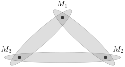
Figure 4.1: Specker’s scenario.

It is worth noting that the impossibility of jointly implementing arbitrary sets of measurements is a key ingredient that enables a demonstration of the nonclassicality of quantum theory in proofs of Bell’s theorem [17] and the Kochen–Specker theorem [10]. A finite set of measurements is called jointly measurable or compatible if there exists a single measurement whose various coarse-grainings recover the original measurements. The problem of characterizing the joint measurability of observables has been studied in the literature [44, 50], and at least the joint measurability of binary qubit observables has been completely characterized [51, 43]. The connection between Bell inequality violations and the joint measurability of observables has also been quantitatively studied [52, 53].

A natural question that arises when thinking about the (in)compatibility of observables is the following: given a set of (in)compatibility relations on a set of vertices representing observables, do they admit a quantum realization? That is, can one write down a positive-operator valued measure (POVM) for each vertex such that the (in)compatibility relations among the vertices are realized by the assigned POVMs? After formally defining these notions, we answer this question in the affirmative by providing an explicit construction of POVMs for any set of (in)compatibility relations.

We will use the terms ‘(not) jointly measurable’ and ‘(in)compatible’ interchangeably in this chapter. Part of our motivation in studying this question comes from the simplest example of joint measurability relations realizable with POVMs but not with projective measurements. As we mentioned, this joint measurability scenario, referred to as Specker’s scenario [28, 29, 30] in Chapter 1, involves three binary measurements that can be jointly measured pairwise but not triplewise: that is, for the set of binary measurements $\{M_{1},M_{2},M_{3}\}$, the (in)compatibility relations are given by the collection of compatible subsets $\{\{M_{1},M_{2}\},\{M_{2},M_{3}\},\{M_{1},M_{3}\}\}$. The remaining nontrivial subset (with at least two observables), namely $\{M_{1},M_{2},M_{3}\}$, is incompatible. This can be pictured as a hypergraph (Fig. 4.1).

In Chapter 1, we showed how Specker’s scenario can be exploited to violate the LSW inequality using a set of three qubit POVMs realizing this scenario [6, 29, 30]. This novel demonstration of contextuality in quantum theory raises the question of whether there exist other scenarios—for example in an observable-based hypergraph approach as in [54, 24]—that do not admit a proof of quantum contextuality using projective measurements, but do admit such a proof using POVMs. A necessary first step towards answering this question is to figure out what compatibility scenarios are realizable in quantum theory. One can then ask whether these scenarios allow nontrivial correlations that rule out noncontextuality [6]. We take this first step by proving that, in principle, all joint measurability hypergraphs are realizable in quantum theory. The realizability of all joint measurability graphs via projective measurements is known [48]. This prompted our question whether all joint measurability hypergraphs are realizable via POVMs. Our positive answer includes joint measurability hypergraphs that do not admit a realization using projective measurements. For our construction, it suffices to consider binary observables on finite-dimensional Hilbert spaces.

4.2 Definitions

POVMs.

A positive-operator valued measure (POVM) on a Hilbert space $\mathcal{H}$ is a mapping $x\mapsto M(x)$ from an outcome set $X$ ($x\in X$) to the set of positive semidefinite operators

$$M(x)\in\mathcal{B}(\mathcal{H}),\quad M(x)\geq 0,$$

such that the POVM elements $M(x)$ sum to the identity operator,

$$\sum_{x\in X}M(x)=I.$$

If $M(x)^{2}=M(x)$ for all $x\in X$, then the POVM becomes a “projection valued measure”, or simply, a projective measurement.

Joint measurability of POVMs.

A finite set of POVMs

$$\{M_{1},\dots,M_{N}\},$$

where measurement $M_{i}$ has outcome set $X_{i}$, is said to be jointly measurable or compatible if there exists a POVM $M$ with outcome set $X_{1}\times X_{2}\times\dots\times X_{N}$ that marginalizes to each $M_{i}$ with outcome set $X_{i}$, meaning that

$$M_{i}(x_{i})=\sum_{x_{1},\ldots,\cancel{x_{i}},\ldots,x_{N}}M(x_{1},\dots,x_{N})$$

for all outcomes $x_{i}\in X_{i}$.

Joint measurability hypergraphs.

A hypergraph consists of a set of vertices $V$, and a family $E\subseteq\{e\mid e\subseteq V\}$ of subsets of $V$ called edges. We think of each vertex as representing a POVM, while an edge models joint measurability of the POVMs it links. Since every subset of a set of compatible measurements should also be compatible, a joint measurability hypergraph should have the property that any subset of an edge is also an edge,

$$e\in E,\>e^{\prime}\subseteq e\implies e^{\prime}\in E.$$

Additionally, we focus on the case where each edge $e$ is a finite subset of $V$. This makes a joint measurability hypergraph into an abstract simplicial complex.

Every set of POVMs on $\mathcal{H}$ has such an associated joint measurability hypergraph. Hence characterizing joint measurability of quantum observables comes down to figuring out their joint measurability hypergraph. Our main result solves the converse problem. Namely, every abstract simplicial complex arises from the joint measurability relations of a set of quantum observables.

4.3 Quantum realization of arbitrary joint measurability structures

Theorem 8.

Every joint measurability hypergraph admits a quantum realization with POVMs.

Proof.

We begin by proving a necessary and sufficient criterion for the joint measurability of $N$ binary POVMs $M_{k}:=\{E^{k}_{+},E^{k}_{-}\}$ of the form

$$E^{k}_{\pm}:=\frac{1}{2}\left(I\pm\eta\Gamma_{k}\right),$$ (4.1)

where the $\Gamma_{k}$ are generators of a Clifford algebra as in the Appendix. The variable $\eta\in[0,1]$ is a purity parameter. Since $\Gamma_{k}^{2}=I$, the eigenvalues of $\Gamma_{k}$ are $\pm 1$, so that $E^{k}_{\pm}$ is indeed positive. The following derivation of a joint measurability criterion is adapted from a proof first obtained in [29], and subsequently revised in [30], for the joint measurability of a set of noisy qubit POVMs. Because $\Gamma_{k}$ is traceless by (4.9), we can recover the purity parameter $\eta$ as

$$\text{Tr}(\Gamma_{k}E^{k}_{\pm})=\pm\frac{\eta}{2}d,$$

so that

$$\eta=\frac{1}{Nd}\sum_{k=1}^{N}\sum_{x_{k}\in X_{k}}\text{Tr}(x_{k}\Gamma_{k}E^{k}_{x_{k}}),$$ (4.2)

where we have introduced one separate outcome $x_{k}\in X_{k}:=\{+1,-1\}$ for each measurement $M_{k}$.

If all $M_{k}=\{E^{k}_{+},E^{k}_{-}\}$ together are jointly measurable, then there exists a joint POVM $M=\{E_{x_{1}\dots x_{N}}\}$ satisfying

$$E^{k}_{x_{k}}=\sum_{x_{1},\ldots\cancel{x_{k}},\ldots x_{N}}E_{x_{1}\dots x_{N}}.$$

Writing $\vec{x}:=(x_{1},\ldots,x_{N})$ and $\vec{\Gamma}:=(\Gamma_{1},\ldots,\Gamma_{N})$, this assumption together with (4.2) implies that

$$\eta =\frac{1}{Nd}\sum_{\vec{x}}\text{Tr}\left[\left(\sum_{k=1}^{N}x_{k}\Gamma_{k}\right)E_{x_{1}\dots x_{N}}\right]$$

$$\leq\frac{1}{Nd}\sum_{\vec{x}}\|\vec{x}\cdot\vec{\Gamma}\|\>\text{Tr}\left[E_{\vec{x}}\right]$$

$$=\frac{1}{N}\|\vec{x}\cdot\vec{\Gamma}\|,$$

where the last step used the normalization $\sum_{\vec{x}}E_{\vec{x}}=I$. Since $(\vec{x}\cdot\vec{\Gamma})^{2}=\sum_{k}X_{k}^{2}=N\cdot I$ by (4.10), we have $\|\vec{x}\cdot\vec{\Gamma}\|=\sqrt{N}$, and therefore

$$\eta\leq\frac{1}{\sqrt{N}},$$

a necessary condition for joint measurability of $M_{k}$. To show that this condition is also sufficient, we consider the joint POVM $M=\{E_{\vec{x}}\}$ given by

$$E_{x_{1}\dots x_{N}}:=\frac{1}{2^{N}}\left(I+\eta\>\vec{x}\cdot\vec{\Gamma}\right).$$ (4.3)

We start by showing that this indeed defines a POVM,

$$E_{x_{1}\dots x_{N}}\geq 0,\quad\sum_{x_{1},\dots,x_{N}}E_{x_{1}\dots x_{N}}=I.$$

Positivity follows again from noting that the eigenvalues of $\vec{x}\cdot\vec{\Gamma}$ are $\pm\sqrt{N}$ by (4.10), and normalization from $\sum_{\vec{x}}\vec{x}\cdot\vec{\Gamma}=0$. Since

$$\sum_{x_{1},\ldots,\cancel{x_{k}},\ldots,x_{N}}E_{x_{1}\dots x_{N}}=\frac{1}{2}\left(I+\eta x_{k}\Gamma_{k}\right)$$

coincides with (4.1), we have indeed found a joint POVM marginalizing to the given $M_{k}$.

Thus $\eta\leq\frac{1}{\sqrt{N}}$ is a necessary and sufficient condition for the joint measurability of $M_{1},\ldots,M_{N}$.

For arbitrary $N$, then, we can construct $N$ POVMs on a Hilbert space of appropriate dimension such that any $N-1$ of them are compatible, whereas all $N$ together are incompatible: simply take $M_{1},\ldots,M_{N}$ from (4.1) for any purity parameter $\eta$ satisyfing

$$\frac{1}{\sqrt{N}}<\eta\leq\frac{1}{\sqrt{N-1}}.$$

For example, $\eta=1/\sqrt{N-1}$ will work. The above reasoning guarantees that all $N$ of them together are not compatible, and also that the $M_{1},\ldots,M_{N-1}$ are compatible. By permuting the labels and observing that the above reasoning did not rely on any specific ordering of the $\Gamma_{k}$, we conclude that any $N-1$ measurements among the $M_{1},\ldots,M_{N}$ are compatible.

What we have established so far is that, if we are given any $N$-vertex joint measurability hypergraph where every subset of $N-1$ vertices is compatible (i.e. belongs to a common edge), but the $N$-vertex set is incompatible, then the above construction provides us with a quantum realization of it. These “Specker-like” hypergraphs are crucial to our construction. For example, for $N=3$, we obtain a simple realization of Specker’s scenario (Fig. 4.1). For $N=2$, we simply obtain a pair of incompatible observables. Given an arbitrary joint measurability hypergraph, the procedure to construct a quantum realization is now the following:

1. Identify the minimal incompatible sets of vertices in the hypergraph. A minimal incompatible set is an incompatible set of vertices such that any of its proper subsets is compatible. In other words, it is a Specker-like hypergraph embedded in the given joint measurability hypergraph.

2. For each minimal incompatible set, construct a quantum realization as above. Vertices that are outside this minimal incompatible set can be assigned a trivial POVM in which one outcome is deterministic, represented by the identity operator $I$. Let $\mathcal{H}_{i}$ denote the Hilbert space on which the minimal incompatible set is realized, where $i$ indexes the minimal incompatible sets.

3. Having thus obtained a quantum representation of each minimal incompatible set, we simply “stack” these together in a direct sum over the Hilbert spaces on which each of the minimal incompatible sets are realized. On this larger direct sum Hilbert space $\mathcal{H}=\oplus_{i}\mathcal{H}_{i}$, we then have a quantum realization of the joint measurability hypergraph we started with.

For any edge $e\in E$, the associated measurements are compatible on every $\mathcal{H}_{i}$, and therefore also on $\mathcal{H}$. On the other hand, every $e^{\prime}\subseteq V$ that is not an edge is contained in some minimal incompatible set (or is itself already minimal), and therefore the associated POVMs are incompatible on some $\mathcal{H}_{i}$, and hence also on $\mathcal{H}$. ∎

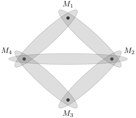
Figure 4.2: A joint measurability hypergraph for $N=4$.

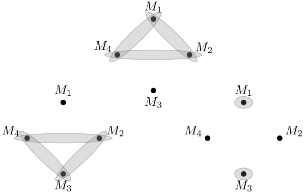
Figure 4.3: Minimal incompatible sets for the joint measurability hypergraph in Fig. 4.2.

4.4 A simple example

To illustrate these ideas, we construct a POVM realization of a simple joint measurability hypergraph that does not admit a representation with projective measurements (Fig. 4.2). This hypergraph can be decomposed into three minimal incompatible sets of vertices (Fig. 4.3). Two of these are Specker scenarios for $\{M_{1},M_{2},M_{4}\}$ and $\{M_{2},M_{3},M_{4}\}$, and the third one is a pair of incompatible vertices $\{M_{1},M_{3}\}$. For the minimal incompatible set $\{M_{1},M_{2},M_{4}\}$, we construct a set of three binary POVMs, $A_{k}\equiv\{A^{k}_{+},A^{k}_{-}\}$ with $k\in\{1,2,4\}$ on a qubit Hilbert space $\mathcal{H}_{1}$ given by

$$A^{k}_{\pm}:=\frac{1}{2}\left(I\pm\frac{1}{\sqrt{2}}\Gamma_{k}\right),$$ (4.4)

where the matrices $\{\Gamma_{1},\Gamma_{2},\Gamma_{4}\}$ can be taken to be the Pauli matrices,

$$\Gamma_{1}=\sigma_{z},\quad\Gamma_{2}=\sigma_{x},\quad\Gamma_{4}=\sigma_{y},$$

similar to (4.8). The remaining vertex $M_{3}$ can be taken to be the trivial POVM $A_{3}=\{0,I\}$ on $\mathcal{H}_{1}$. A similar construction works for the second Specker scenario $\{M_{2},M_{3},M_{4}\}$ by setting $B_{k}:=\{B^{k}_{+},B^{k}_{-}\}$ with $k\in\{2,3,4\}$ to be

$$B^{k}_{\pm}:=\frac{1}{2}\left(I\pm\frac{1}{\sqrt{2}}\Gamma_{k}\right),$$ (4.5)

where

$$\Gamma_{2}=\sigma_{z},\quad\Gamma_{3}=\sigma_{x},\quad\Gamma_{4}=\sigma_{y}$$

act on another qubit Hilbert space $\mathcal{H}_{2}$. The remaining vertex $M_{1}$ can be assigned the trivial POVM, $B_{1}=\{0,I\}$. The third minimal incompatible set $\{M_{1},M_{3}\}$ can similarly be obtained on another qubit Hilbert space $\mathcal{H}_{3}$ as $C_{k}:=\{C^{k}_{+},C^{k}_{-}\}$, with $k\in\{1,3\}$, given by

$$C^{k}_{\pm}:=\frac{1}{2}(I\pm\Gamma_{k}),$$ (4.6)

where now e.g. $\Gamma_{1}=\sigma_{z}$ and $\Gamma_{3}=\sigma_{x}$. The remaining vertices $M_{2}$ and $M_{4}$ can both be assigned the trivial POVM $C_{2}=C_{4}:=\{0,I\}$ on $\mathcal{H}_{3}$.

In the direct sum Hilbert space $\mathcal{H}:=\mathcal{H}_{1}\oplus\mathcal{H}_{2}\oplus\mathcal{H}_{3}$, we then have a POVM realization of the joint measurability hypergraph of Fig. 4.2, given by

$$M^{k}_{\pm}:=A^{k}_{\pm}\oplus B^{k}_{\pm}\oplus C^{k}_{\pm}.$$

4.5 Chapter summary

We have shown, by construction, that any conceivable set of (in)compatibility relations for any number of quantum measurements can be realized using a set of binary POVMs. Our result thus demonstrates that quantum theory is not constrained to admit only a restricted set of (in)compatibility relations, such as those where pairwise compatibility $\Leftrightarrow$ global compatibility, which is the case with projective measurements. Indeed, quantum theory admits all possible (in)compatibility relations. With respect to (in)compatibility relations, therefore, quantum theory is as far away from classical theories (where there are no incompatibilities) as possible. By “classical theories” we mean those where all measurements can be jointly implemented.

Although our simple construction works for all joint measurability hypergraphs, it is probably not the most efficient one for a given joint measurability hypergraph: for Fig. 4.2, our representation lives on a six-dimensional Hilbert space. For a joint measurability hypergraph with a fixed number of vertices, the dimension of the Hilbert space $\mathcal{H}$ on which our construction is realized depends on the number of minimal incompatible sets in the hypergraph: that is, $\dim\mathcal{H}=\sum_{i}\dim\mathcal{H}_{i}$, where $\mathcal{H}_{i}$ is the Hilbert space on which the $i$th minimal incompatible set is realized. It remains open what the most efficient construction—requiring the smallest Hilbert space dimension—for a given joint measurability hypergraph is. Our result captures all conceivable (in)compatibility relations within the framework of quantum theory, thus shedding light on the structure of quantum theory and what it really allows us to do.

Appendix: Clifford algebras

A Clifford algebra consists of a finite set of hermitian matrices $\Gamma_{1},\ldots,\Gamma_{N}$ satisfying the relations

$$\Gamma_{j}\Gamma_{k}+\Gamma_{k}\Gamma_{j}=2\delta_{jk}I,$$ (4.7)

Clifford algebras are the mathematical structure behind the definition of spinors and the Dirac equation [55]. They can be constructed recursively as follows [55, Sec. 16.3]. Given $\Gamma_{1},\dots,\Gamma_{N}$ living on a Hilbert space $\mathcal{H}_{N}$, one obtains $\Gamma_{1},\ldots,\Gamma_{N+2}$ on $\mathcal{H}_{N}\otimes\mathbb{C}^{2}$ by the following rules.

1. For each $i=1,\dots,N$, substitute

   $$\Gamma_{i}\rightarrow\Gamma_{i}\otimes\sigma_{z}.$$

2. Further, define

   $$\Gamma_{N+1}:=I\otimes\sigma_{x},\quad\Gamma_{N+2}:=I\otimes\sigma_{y}.$$

It is easy to show that if the original $\Gamma_{i}$ satisfy (4.7), then so do the new ones. One can simply start the recursion with $\Gamma_{1}=1$ on the one-dimensional Hilbert space $\mathcal{H}_{1}:=\mathbb{C}$, and then apply the construction as often as necessary to obtain any finite number of matrices satisfying (4.7). For example, a single iteration gives the Pauli matrices

$$\Gamma_{1}=\sigma_{z},\quad\Gamma_{2}=\sigma_{x},\quad\Gamma_{3}=\sigma_{y},$$ (4.8)

while after two iterations one has

$$\Gamma_{1}=\sigma_{z}\otimes\sigma_{z},\quad\Gamma_{2}=\sigma_{x}\otimes\sigma_{z},$$

$$\Gamma_{3}=\sigma_{y}\otimes\sigma_{z},\quad\Gamma_{4}=I\otimes\sigma_{x},\quad\Gamma_{5}=I\otimes\sigma_{y}.$$

The Clifford algebra relations (4.7) have many interesting consequences. For example for $N\geq 2$, one has for any $k$ and $j\neq k$,

$$\text{Tr}(\Gamma_{k}) =\text{Tr}(\Gamma_{k}\Gamma_{j}\Gamma_{j})=-\text{Tr}(\Gamma_{j}\Gamma_{k}\Gamma_{j})$$

$$=-\text{Tr}(\Gamma_{k}\Gamma_{j}\Gamma_{j})=-\text{Tr}(\Gamma_{k}),$$

so that

$$\text{Tr}(\Gamma_{k})=0.$$ (4.9)

Another consequence is that

$$\left(\sum_{k}X_{k}\Gamma_{k}\right)^{2}=\left(\sum_{k}X_{k}^{2}\right)\cdot I$$ (4.10)

for arbitrary real coefficients $X_{k}$.

Chapter 5 Fine’s theorem and its status in tests of noncontextuality

In this chapter, we provide a characterization of noncontextual models which fall within the ambit of Fine’s theorem[56, 57]. In particular, we make explicit the equivalence between the existence of three notions: a joint probability distribution over the outcomes of all the measurements considered, a measurement-noncontextual and outcome-deterministic (or KS-noncontextual) model for these measurements, and a measurement-noncontextual and factorizable model for them. A KS-inequality, therefore, is implied by each of these three notions. Following this characterization of noncontextual models that fall within the ambit of Fine’s theorem, non-factorizable noncontextual models which lie outside the domain of Fine’s theorem are considered. While outcome determinism for projective (sharp) measurements in quantum theory can be shown to follow from the assumption of preparation noncontextuality, as we did in Chapter 1, such a justification is not available for nonprojective (unsharp) measurements which ought to admit outcome-indeterministic response functions. The Liang-Spekkens-Wiseman (LSW) inequality is an example of a noncontextuality inequality that should hold in any noncontextual model of quantum theory without assuming factorizability. Three other noncontextuality inequalities, which turn out to be equivalent to the LSW inequality under relabellings of measurement outcomes, are derived for Specker’s scenario. We also characterize the polytope of correlations admissible in this scenario, given the operational equivalences between measurements (often called the “no-disturbance” condition in the literature on KS-contextuality).

This chapter is based on work reported in Ref. [58].

5.1 Introduction

In attempts to provide a more complete description of reality than operational quantum theory in terms of a noncontextual ontological model, it is almost always assumed that whatever the ontic state $\lambda$ is, it must specify the outcomes of measurements exactly (an assumption called outcome determinism) and any operational unpredictability in the measurement outcomes is on account of coarse-graining over these ontic states $\lambda$. This chapter concerns itself with what can still be said about noncontextuality if outcome determinism is not assumed: the ontic state is not always required to fix the outcomes of measurements but only their probabilities. The physical motivation for this becomes clear once the following questions are asked:

1. Do there exist noncontextual ontological models of quantum theory where the ontic state $\lambda$ fixes the outcomes of measurements?
   

   The Kochen-Specker theorem [10] rules out this possibility. Let us now remove the requirement of outcome determinism, namely, that $\lambda$ fix the outcomes of measurements, and ask the question:

2. Do there exist noncontextual ontological models of quantum theory where the ontic state $\lambda$ fixes the probabilities of outcomes of measurements?
   

   The Kochen-Specker theorem [10] is silent on this question since it presumes the ontic state $\lambda$ must fix the outcomes of (projective) measurements. This question is most naturally addressed in the framework of generalized noncontextuality due to Spekkens [6].

It is well-known that, in contrast to the Kochen-Specker theorem [10], Bell’s theorem [23, 59] does not require an assumption that the ontic state $\lambda$ fixes the outcomes of the measurements. This becomes particularly clear in view of Fine’s theorem [56, 57] that, in a Bell scenario, a locally deterministic model [17] exists if and only if a locally causal (or ‘Bell-local’) model [23, 59] exists, and how this is equivalent to requiring the existence of a joint probability distribution over outcomes of all the measurements considered in a Bell scenario. Hence, even if the outcomes are only determined probabilistically by $\lambda$ in the local hidden variable model, Bell’s theorem holds. The key issue in Bell scenarios is factorizability: the conditional independence of the outcomes of spacelike separated measurements given the ontic state $\lambda$ of the system,

$$\xi(X_{1},\dots,X_{N}|M_{1},\dots,M_{N},\lambda)$$ (5.1)

$$= \xi(X_{1}|M_{1},\lambda)\xi(X_{2}|M_{2},\lambda)\dots\xi(X_{N}|M_{N},\lambda),$$

where $X_{i}$ labels the outcome of measurement $M_{i}$ performed by the $i$th party, $i\in\{1,\dots,N\}$. All these response functions may be outcome-indeterministic, i.e., $\xi\in[0,1]$. Indeed, factorizability is a necessary consequence of any set of assumptions that may be used to derive Bell’s theorem [59].

On the other hand, things are not as straightforward for contextuality [28, 13, 10]. Mathematically, both Bell-local models and KS-noncontextual models rely on the existence of a joint probability distribution over all measurement outcomes in a given scenario such that this distribution reproduces the observed statistics as marginals. Proofs of the KS theorem that rely on uncolorability (such as the original proof in Ref. [10]) are such that there exists no joint distribution at all, given any set of observed marginals. These proofs are often termed state-independent since they do not rely on preparing particular quantum states on which the measurement statistics are considered: any quantum state works. Weaker proofs of the KS theorem (such as the one in Ref. [35]) are such that there exist joint distributions for some, but not all, sets of observed marginals: there exist sets of observable marginals that admit no joint distribution and therefore violate some KS inequality arising from requiring the existence of a joint distribution. These proofs are often termed state-dependent since they rely on preparing particular quantum states that lead to marginal statistics violating a KS inequality. The state-dependent proofs of KS-contextuality are therefore analogous to proofs of Bell’s theorem.

Given this correspondence between Bell’s theorem and the KS theorem, one may ask whether the assumption of outcome determinism is really required in the KS theorem and whether the KS theorem excludes also all outcome-indeterministic noncontextual models on account of Fine’s theorem.

The outcome-indeterministic noncontextual models excluded by the KS theorem are precisely the ones where factorizability holds. However, in the absence of spacelike separation between measurements one does not have a compelling physical justification to assume that measurement outcomes are conditionally independent of each other (and the remote measurement settings) given the ontic state $\lambda$. The physical meaning of factorizability is this: that the measurement outcomes do not have any correlations that are not due to the ontic state $\lambda$ of the system. One could, on the other hand, imagine an adversarial situation where two measurement outcomes are correlated—which is physically possible if they are not spacelike separated—and this correlation is not mediated only by the ontic state $\lambda$ of the system but is perhaps encoded in the degrees of freedom of the measurement apparatus by an adversary who wants to convince the experimenter that something nonclassical is going on (in the sense of KS-contextuality) but, really, it is correlated noise that’s doing all the work of violating a KS inequality. The LSW inequality [29, 30] is an example of a noncontextuality inequality that takes this possibility into account and raises the bar for what correlations count as nonclassical. This is why we need to consider noncontextual models which are not factorizable. Since all KS-noncontextual models are factorizable on account of Fine’s theorem, noncontextual models which are not factorizable are exclusively taken into account only in the generalized definition of noncontextuality [6]. This realization is a key conceptual insight of this chapter, pointing to the necessity of revising the traditional analyses of KS-noncontextuality to accommodate the generalized notion of noncontextuality [6]. To be clear, by outcome determinism and factorizability, we mean the following:

Outcome determinism

is the assumption that every response function in the ontological model is deterministic, i.e., $\xi(k|M,\lambda)\in\{0,1\}$ for all measurement events $[k|M]$ and for all $\lambda\in\Lambda$.

Ontological models where outcome determinism doesn’t hold are called outcome indeterministic. Of the class of outcome-indeterministic ontological models, the ones that are related to outcome-deterministic models via Fine’s theorem are those satisfying factorizability:

Factorizability

is the assumption that for every jointly measurable set of measurements $\{M_{s}^{(S)}|s\in S\}$, the response function for every outcome of a joint measurement $M_{S}$ is the product of the response functions of measurements in the jointly measurable set: $\xi(k_{S}|M_{S},\lambda)=\prod_{s\in S}\xi(k_{s}|M_{s}^{(S)},\lambda)$. Note that $k_{S}\in\mathcal{K}_{M_{S}}$ and $k_{s}\in\mathcal{K}_{M_{s}^{(S)}}$, where $\mathcal{K}_{M_{S}}$ is the Cartesian product of the outcome sets $\mathcal{K}_{M_{s}^{(S)}},s\in S$.

It should be clear that, for a given set of measurements $\{M_{1},\dots,M_{N}\}$ with jointly measurable subsets $S\subset\{1,\dots,N\}$, outcome determinism implies factorizability, but not conversely. Outcome determinism requires that $\xi(k_{S}|M_{S},\lambda)\in\{0,1\}$ for all $S$, and $\xi(k_{s}|M_{s}^{(S)},\lambda)\in\{0,1\}$ for all $s\in S$. $\xi(k_{S}|M_{S},\lambda)=1$ means that $\xi(k_{s}|M_{s}^{(S)},\lambda)=\sum_{k_{s^{\prime}}:s^{\prime}\neq s}\xi(k_{S}|M_{S},\lambda)=1$ for all $s\in S$ and $\xi(k_{S}|M_{S},\lambda)=0$ means that $\xi(k_{s}|M_{s}^{(S)},\lambda)=\sum_{k_{s^{\prime}}:s^{\prime}\neq s}\xi(k_{S}|M_{S},\lambda)=0$ for at least one $s\in S$. All in all, we have $\xi(k_{S}|M_{S},\lambda)=\prod_{s\in S}\xi(k_{s}|M_{s}^{(S)},\lambda)$, which is what factorizability requires. That the converse is not true is easily seen by noting that one can have factorizability without requiring $\xi(k_{S}|M_{S},\lambda)\in\{0,1\}$ or $\xi(k_{s}|M_{s}^{(S)},\lambda)\in\{0,1\}$.

Just as local causality does not require the assumption of outcome determinism, a good definition of noncontextuality should also not appeal to outcome determinism (or even factorizability). Experimental violations of Bell inequalities certify a kind of nonclassicality independent of the truth of quantum theory, a feature that makes Bell inequality violations an invaluable resource in device-independent protocols [60]. In contrast, KS-noncontextuality has to refer to projective (sharp) measurements in quantum theory and assume outcome-determinism for them in order to obtain a KS-inequality: neither of these is needed in a Bell-local model. The generalized notion of noncontextuality offers the possibility of talking about noncontextuality without making the assumption that the operational theory is quantum theory. The present chapter, however, restricts itself to generalized noncontextuality for operational quantum theory.

In the next section, we will see how factorizability - although it’s a physically motivated assumption in locally causal models - is not well-motivated physically in the general case of noncontextual models. Fine’s theorem thus serves to delineate a mathematical boundary between KS-noncontextual models and measurement noncontextual models which are not factorizable.

5.2 Fine’s theorem for noncontextual models

Theorem 9.

Given a set of measurements $\{M_{1},\dots,M_{N}\}$ with jointly measurable subsets $S\subset\{1,\dots,N\}$, where each measurement $M_{s},s\in S$, takes values labelled by $k_{s}\in\mathcal{K}_{M_{s}}$, the following propositions are equivalent:

1. For a given preparation $P\in\mathcal{P}$ of the system there exists a joint probability distribution $p(k_{1},\dots,k_{N}|P)$ that recovers the marginal statistics for jointly measurable subsets predicted by the operational theory (such as quantum theory) under consideration, i.e., $\forall S\subset\{1,\dots,N\}$, $p(k_{S}|M_{S};P)=\sum_{k_{i}:i\notin S}p(k_{1},\dots,k_{N}|P)$, where $k_{S}\in\mathcal{K}_{M_{S}}$.

2. There exists a measurement-noncontextual and outcome-deterministic, i.e. KS-noncontextual, model for these measurements.

3. There exists a measurement-noncontextual and factorizable model for these measurements.

Proof. The proof of equivalence of the three propositions proceeds as follows: Proposition 3 $\Rightarrow$ Proposition 1, Proposition 1 $\Rightarrow$ Proposition 2, Proposition 2 $\Rightarrow$ Proposition 3.

Proposition 3 $\Rightarrow$ Proposition 1:

By Proposition 3, the assumption of measurement noncontextuality requires that the single-measurement response functions in the model be of the form $\xi(k_{i}|M_{i};\lambda)\in[0,1]$, so that each response function is independent of the contexts—jointly measurable subsets $S$—that the corresponding measurement may be a part of. Of course, the assumption of measurement noncontextuality only applies once it is verified that for any $P\in\mathcal{P}$ the operational statistics $p(k_{i}|M_{i};P)$ of measurement $M_{i}$ is the same across all the jointly measurable subsets, $S$, in which it appears. The response function is therefore conditioned only by $M_{i}$ and the ontic state $\lambda$ associated with the system (and not on the jointly measurable subset $S$ that $M_{i}$ may be a part of). Proposition 3 requires, in addition, factorizability, i.e., for all jointly measurable subsets $S\subset\{1,\dots,N\}$,

$$\xi(k_{S}|M_{S};\lambda)=\prod_{s\in S}\xi(k_{s}|M_{s};\lambda).$$

Factorizability amounts to the assumption that the correlations between measurement outcomes are established only via the ontic state of the system—the measurement outcomes do not “talk” to each other except via $\lambda$. Now define

$$\xi(k_{1},\dots,k_{N}|\lambda)\equiv\prod_{i=1}^{N}\xi(k_{i}|M_{i};\lambda),$$ (5.2)

so that marginalizing this distribution over $k_{i}$, $i\notin S$, yields $\xi(k_{S}|M_{S};\lambda)$ for every jointly measurable subset $S\subset\{1,\dots,N\}$.

Assuming the ontological model reproduces the operational statistics, there must exist a probability distribution $\mu(\lambda|P)$ for any $P\in\mathcal{P}$, such that

$$\sum_{\lambda\in\Lambda}\xi(k_{S}|M_{S};\lambda)\mu(\lambda|P)=p(k_{S}|M_{S};P).$$ (5.3)

Then define

$$p(k_{1}\dots k_{N}|P)\equiv\sum_{\lambda\in\Lambda}\xi(k_{1}\dots k_{N}|\lambda)\mu(\lambda|P),$$ (5.4)

which marginalizes on $k_{S}$ to

$$p(k_{S}|P) = \sum_{k_{i}:i\notin S}p(k_{1}\dots k_{N}|P)$$ (5.5)

$$= \sum_{\lambda\in\Lambda}\sum_{k_{i}:i\notin S}\xi(k_{1}\dots k_{N}|\lambda)\mu(\lambda|P)$$ (5.6)

$$= \sum_{\lambda\in\Lambda}\xi(k_{S}|M_{S};\lambda)\mu(\lambda|P)$$ (5.7)

$$= p(k_{S}|M_{S};P).$$ (5.8)

Thus, Proposition 3 $\Rightarrow$ Proposition 1.

Proposition 1 $\Rightarrow$ Proposition 2:

By Proposition 1, for a given $P\in\mathcal{P}$ there exists a $p(k_{1}\dots k_{N}|P)$ such that $p(k_{S}|M_{S};P)=\sum_{k_{i}:i\notin S}p(k_{1}\dots k_{N}|P)$, for all jointly measurable subsets $S\subset\{1,\dots,N\}$. Now, there exists a probability distribution over the ontic state space, $\mu(\lambda|P)$, such that

$$p(k_{1}\dots k_{N}|P)=\sum_{\lambda\in\Lambda}\xi(k_{1}\dots k_{N}|\lambda)\mu(\lambda|P)$$ (5.9)

where $\xi(k_{1}\dots k_{N}|\lambda)\in\{0,1\}$. This is possible because any probability distribution can be decomposed as a convex sum over deterministic distributions. Also, $p(k_{j}|M_{j};P)=\sum_{k_{i}:i\neq j}p(k_{1},\dots,k_{N}|P)$, so

$$p(k_{j}|M_{j};P)=\sum_{\lambda\in\Lambda}\mu(\lambda|P)\sum_{k_{i}:i\neq j}\xi(k_{1}\dots k_{N}|\lambda),$$ (5.10)

which allows the definition

$$\xi(k_{j}|M_{j};\lambda)\equiv\sum_{k_{i}:i\neq j}\xi(k_{1}\dots k_{N}|\lambda)\in\{0,1\},\forall j\in\{1\dots N\}.$$ (5.11)

Since these are deterministic distributions,

$$\xi(k_{1}\dots k_{N}|\lambda)=\prod_{j=1}^{N}\xi(k_{j}|M_{j};\lambda).$$ (5.12)

Finally,

$$p(k_{S}|M_{S};P)=\sum_{\lambda\in\Lambda}\mu(\lambda|P)\prod_{s\in S}\xi(k_{s}|M_{s};\lambda),$$ (5.13)

so there exists a measurement-noncontextual and outcome-deterministic model, i.e., Proposition 1 $\Rightarrow$ Proposition 2.

Proposition 2 $\Rightarrow$ Proposition 3:

By Proposition 2, $\xi(k_{i}|M_{i};\lambda)\in\{0,1\},\forall i\in\{1\dots N\}$, such that

$$p(k_{S}|M_{S};P)=\sum_{\lambda\in\Lambda}\mu(\lambda|P)\prod_{s\in S}\xi(k_{s}|M_{s};\lambda),$$ (5.14)

$\forall$ jointly measurable subsets $S\subset\{1\dots N\}$. Clearly, this model is also a measurement-noncontextual and factorizable model because the assumption of outcome-determinism implies factorizability:

$$\xi(k_{S}|M_{S};\lambda)=\prod_{s\in S}\xi(k_{s}|M_{s};\lambda).$$ (5.15)

Note that this theorem itself is not new, but this particular reading of it in the framework of generalized noncontextuality is new. In particular, the purpose of this restatement is to highlight why outcome-determinism is not an assumption that can be taken for granted in noncontextual ontological models. Versions of this theorem have appeared in the literature following Fine’s original insight [56, 57]. The fact that Proposition 2 implies Proposition 1 has been shown earlier in Ref. [29]. A similar result in the language of sheaf theory can be found Ref. [54], where the authors point out factorizability as the underlying assumption in Bell-local and KS-noncontextual models: in effect they show the equivalence of Proposition 1 and Proposition 3. The sense in which Ref. [54] refers to ‘non-contextuality’ is the notion of KS-noncontextuality, and while it is possible to provide a unified account of Bell-locality and KS-noncontextuality at a mathematical level, the generalized notion of noncontextuality [6] does not admit such an account. In particular, their definition of ‘non-contextuality’ is stronger than the Spekkens’ definition of measurement noncontextuality. Indeed, as we have amply demonstrated in Chapter 1, generalized noncontextuality subsumes KS-noncontextuality but is not equivalent to it.

Fine’s theorem for Bell scenarios.

Translating the preceding notions from noncontextual models to Bell-local models amounts to replacing ‘measurement-noncontextual and outcome-deterministic’ by ‘locally deterministic’ and ‘measurement-noncontextual and factorizable’ by ‘locally causal’. Consider the case of two-party Bell scenarios for simplicity, although the same considerations extend to general multiparty Bell scenarios in a straightforward manner. A two-party Bell scenario consists of measurements $\{M_{1},\dots,M_{N}\}$, where $\{M_{1},\dots,M_{n}\}$, $n<N-1$, are the measurement settings available to one party, say Alice, and $\{M_{n+1},\dots,M_{N}\}$ are the measurement settings available to the other party, say Bob. The outcomes are denoted by $k_{i}\in\mathcal{K}_{M_{i}}$ for the respective measurement settings $M_{i}$. The jointly measurable subsets are given by $S\in\{\{i,j\}|i\in\{1,\dots,n\},j\in\{n+1,\dots,N\}\}$. Bell’s assumption of local causality captures the notion of a measurement noncontextual and factorizable model:

$$p(k_{S}|M_{S};P)$$ (5.16)

$$= p(k_{i},k_{j}|M_{i},M_{j};P)$$

$$= \sum_{\lambda\in\Lambda}\xi(k_{i}|M_{i},\lambda)\xi(k_{j}|M_{j},\lambda)\mu(\lambda|P).$$ (5.17)

Once factorizability is justified from Bell’s assumption of local causality in this manner, Fine’s theorem ensures that – so far as the existence of hidden variable models is concerned – it is irrelevant whether the response functions for the measurement outcomes are deterministic or indeterministic. One does not need to worry about whether outcome-determinism for measurements is justified in Bell scenarios precisely because factorizability along with Fine’s theorem absolves one of the need to provide such a justification. The crucial point, then, is the validity of factorizability in the more general case of noncontextual models. In general, factorizability is not justified in noncontextual models and, following Spekkens, one must distinguish between the issue of noncontextuality and that of outcome-determinism when considering ontological models of an operational theory [6]. If the goal is – as it should be – to obtain an experimental test of noncontextual models independent of the truth of quantum theory, then one needs to derive noncontextuality inequalities that do not rely on outcome-determinism at all. This is because Fine’s theorem for noncontextual models is of limited applicability – namely, outcome-indeterministic response functions which satisfy factorizability are shown by it to achieve no more generality than is already captured by outome-deterministic response functions in a KS-noncontextual model. Outcome-indeterministic response functions that do not satisfy factorizability are not taken into account in a KS-noncontextual model.

For ontological models of operational quantum theory, outcome-determinism for sharp (projective) measurements can be shown to follow from the assumption of preparation noncontextuality [6]. Such a justification is not available for unsharp (nonprojective) measurements, which should therefore be represented by outcome-indeterministic response functions. This issue has been discussed at length by Spekkens and the reader is referred to Ref. [42] for why and how this must be so. Therefore, to consider noncontextuality for unsharp measurements in full generality the noncontextuality inequalities of interest are those which do not assume factorizability. An example is the LSW inequality for Specker’s scenario [29] that does not rely on factorizability, although it does use the assumption of outcome determinism for sharp (projective) measurements. The LSW inequality has been shown to be violated by quantum predictions [30], thus ruling out noncontextual models of quantum theory without invoking factorizability. Note that the distinction between sharp and unsharp measurements is not part of the definition of a Bell-local model and one never has to worry about this distinction to derive Bell’s theorem. This distinction, however, becomes relevant for noncontextual models of quantum theory, where the words ‘sharp’ and ‘unsharp’ have a clear meaning, the former referring to projective measurements and the latter to nonprojective measurements.

In the next section, the polytope of correlations admissible in Specker’s scenario is characterized.

5.3 Correlations in Specker’s scenario

In this section three noncontextuality inequalities relevant to the correlations in Specker’s scenario are derived. They are shown to be equivalent to the known LSW inequality under relabelling of measurement outcomes. This scenario involves three binary measurements, $\{M_{1},M_{2},M_{3}\}$, which are pairwise jointly measurable with outcomes labelled by $X_{i}\in\{0,1\}$ for $i\in\{1,2,3\}$. The statistics involved in Specker’s scenario for a given preparation $P\in\mathcal{P}$ can be understood as a set of $12$ probabilities, $4$ for each pairwise joint measurement $M_{ij}$,

$$\mathcal{S}\equiv\{p(X_{i}X_{j}|M_{ij};P)|X_{i},X_{j}\in\{0,1\},i,j\in\{1,2,3\},i<j\},$$ (5.18)

subject to the obvious constraints of positivity,

$$p(X_{i}X_{j}|M_{ij};P)\geq 0\quad\forall X_{i},X_{j},M_{ij},$$ (5.19)

and normalization,

$$\sum_{X_{i},X_{j}}p(X_{i}X_{j}|M_{ij};P)=1\quad\forall M_{ij}.$$ (5.20)

In addition to positivity and normalization, the statistics is assumed to obey the following condition:

$$\sum_{X_{j}}p(X_{i}X_{j}|M_{ij};P)$$ (5.21)

$$= \sum_{X_{k}}p(X_{i}X_{k}|M_{ik};P)$$

$$\equiv p(X_{i}|M_{i};P),$$ (5.22)

for all $i<j,k$ where $i,j,k\in\{1,2,3\}$. Denoting

$$\sum_{X_{j}}p(X_{i}X_{j}|M_{ij};P)\equiv p(X_{i}|M_{i}^{j};P),$$

and

$$\sum_{X_{k}}p(X_{i}X_{k}|M_{ik};P)\equiv p(X_{i}|M_{i}^{k};P),$$

the condition becomes

$$p(X_{i}|M_{i}^{j};P)=p(X_{i}|M_{i}^{k};P)\equiv p(X_{i}|M_{i};P).$$ (5.23)

That is, the statistics of $M_{i}^{j}$, which is obtained by marginalizing the statistics of joint measurement $M_{ij}$, is identical to the statistics of $M_{i}^{k}$, which is obtained by marginalizing the statistics of joint measurement $M_{ik}$. If what has been measured is indeed a unique observable $M_{i}$ then its statistics relative to any preparation $P\in\mathcal{P}$ should remain the same across joint measurements with different observables $M_{j}$ and $M_{k}$. Failure to meet this condition implies a failure of joint measurability: then one can distinguish between $M_{i}^{j}$ and $M_{i}^{k}$ from their statistics relative to some preparation and they would therefore correspond to two different marginal observables $M_{i}^{j}$ and $M_{i}^{k}$ rather than a unique observable $M_{i}$. This condition, $M_{i}^{j}\simeq M_{i}^{k}\simeq M_{i}$, is often called the no-disturbance condition in the literature on contextuality. Operational quantum theory obeys the no-disturbance condition for joint measurements of generalized observables (which need not be projective or sequential).

5.3.1 Kochen-Specker (KS) inequalities for Specker’s scenario

The four necessary and sufficient inequalities characterizing correlations which admit a KS-noncontextual model in Specker’s scenario are given by:

$$R_{3}\equiv p(X_{1}\neq X_{2}|M_{12},P)+p(X_{2}\neq X_{3}|M_{23},P)+p(X_{1}\neq X_{3}|M_{13},P)\leq 2,$$ (5.24)

and

$$R_{0}\equiv p(X_{1}\neq X_{2}|M_{12},P)-p(X_{2}\neq X_{3}|M_{23},P)-p(X_{1}\neq X_{3}|M_{13},P)\leq 0,$$ (5.25)

$$R_{1}\equiv p(X_{2}\neq X_{3}|M_{23},P)-p(X_{1}\neq X_{3}|M_{13},P)-p(X_{1}\neq X_{2}|M_{12},P)\leq 0,$$ (5.26)

$$R_{2}\equiv p(X_{1}\neq X_{3}|M_{13},P)-p(X_{1}\neq X_{2}|M_{12},P)-p(X_{2}\neq X_{3}|M_{23},P)\leq 0.$$ (5.27)

These inequalities have earlier appeared in Ref. [61]. A derivation is provided in the Appendix at the end of this chapter. Further, these inequalities exhibit a curious property that no two of them can be violated by the same set of experimental statistics:

Lemma 2.

There exists no set of distributions $\{p(X_{i},X_{j}|M_{ij},P)|(ij)\in\{(12),(23),(13)\}\}$ that can violate any two of the four KS inequalities simultaneously.

Proof. Denoting $w_{12}\equiv p(X_{1}\neq X_{2}|M_{12},P)$, $w_{23}\equiv p(X_{2}\neq X_{3}|M_{23},P)$, and $w_{13}\equiv p(X_{1}\neq X_{3}|M_{13},P)$, the four KS inequalities can be rewritten as:

$$R_{3}\equiv w_{12}+w_{23}+w_{13}\leq 2,$$ (5.28)

$$R_{0}\equiv w_{12}-w_{23}-w_{13}\leq 0,$$ (5.29)

$$R_{1}\equiv w_{23}-w_{13}-w_{12}\leq 0,$$ (5.30)

$$R_{2}\equiv w_{13}-w_{23}-w_{12}\leq 0.$$ (5.31)

Now, violation of each of these is equivalent to the following, since $0\leq w_{12},w_{23},w_{13}\leq 1$:

$$R_{3}>2\Leftrightarrow w_{12}+w_{23}+w_{13}>2,$$

$$R_{0}>0\Leftrightarrow w_{12}>w_{23}+w_{13}\Rightarrow w_{12}+w_{23}+w_{13}<2,$$

$$R_{1}>0\Leftrightarrow w_{23}>w_{12}+w_{13}\Rightarrow w_{12}+w_{23}+w_{13}<2$$

$$\text{ and }w_{12}<w_{23}-w_{13},$$

$$R_{2}>0\Leftrightarrow w_{13}>w_{12}+w_{23}\Rightarrow w_{12}+w_{23}+w_{13}<2$$

$$\text{ and }w_{12}<w_{13}-w_{23}.$$

It follows that violation of each inequality above is in conflict with a violation of each of the other three inequalities. Hence, there exist no conceivable measurement statistics that violate any two of the four KS inequalities simultaneously.

5.3.2 Noncontextuality (NC) inequalities for Specker’s scenario

Consider the predictability of each measurement $M_{k}$ defined as:

$$\eta_{M_{k}}\equiv\max_{P}\{2\max_{X_{k}}p(X_{k}|M_{k},P)-1\},$$ (5.32)

where $P\in\mathcal{P}$ is any preparation of the system. Assuming the three measurements in Specker’s scenario have the same predictability $\eta_{0}\equiv\eta_{M_{1}}=\eta_{M_{2}}=\eta_{M_{3}}$, the following noncontextuality inequalities hold:

LSW inequality

$$R_{3}=p(X_{1}\neq X_{2}|M_{12},P)+p(X_{2}\neq X_{3}|M_{23},P)+p(X_{1}\neq X_{3}|M_{13},P)\leq 3-\eta_{0},$$ (5.33)

Three more inequalities

$$R_{0}=p(X_{1}\neq X_{2}|M_{12},P)-p(X_{2}\neq X_{3}|M_{23},P)-p(X_{1}\neq X_{3}|M_{13},P)\leq 1-\eta_{0},$$ (5.34)

$$R_{1}=p(X_{2}\neq X_{3}|M_{23},P)-p(X_{1}\neq X_{3}|M_{13},P)-p(X_{1}\neq X_{2}|M_{12},P)\leq 1-\eta_{0},$$ (5.35)

$$R_{2}=p(X_{1}\neq X_{3}|M_{13},P)-p(X_{1}\neq X_{2}|M_{12},P)-p(X_{2}\neq X_{3}|M_{23},P)\leq 1-\eta_{0}.$$ (5.36)

These inequalities are derived in the Appendix. Note that violation of each of these inequalities implies the violation of the corresponding KS inequalities (recovered for $\eta_{0}=1$), but not conversely.

Lemma 3.

There exists no set of distributions $\{p(X_{i},X_{j}|M_{ij},P)|(ij)\in\{(12),(23),(13)\}\}$ that can violate any two of the four NC inequalities simultaneously.

Proof. The proof trivially follows from Lemma 2, since violation of any NC inequality implies violation of the corresponding KS inequality.

The predictability, $\eta_{0}$, quantifies how predictable a measurement can be made in a variation over preparations: KS inequalities make sense only when $\eta_{0}=1$, i.e., it is possible to find a preparation which makes a given measurement perfectly predictable, a condition which is naturally satisfied by sharp (projective) measurements in quantum theory. For the case of unsharp measurements, $\eta_{0}<1$, and the noncontextuality inequalities take this into account. When $\eta_{0}=0$, that is, when the measurement outcomes are uniformly random (or completely unpredictable), the upper bounds in the noncontextuality inequalities become trivial and a noncontextual model is always possible: simply ignore the system and toss a fair coin to decide whether to output $(X_{i}=0,X_{j}=1)$ or $(X_{i}=1,X_{j}=0)$ when a pair of measurements $\{M_{i},M_{j}\}$ is jointly implemented,

$$p(X_{i},X_{j}|M_{ij},P)=\frac{1}{2}\left(\delta_{X_{i},0}\delta_{X_{j},1}+\delta_{X_{i},1}\delta_{X_{j},0}\right).$$ (5.37)

Clearly, $R_{3}=3$ for this, and $\eta_{0}=0$ since the marginal for each measurement $M_{i}$ is uniformly random independent of the preparation, so the LSW inequality cannot be violated. This admits a noncontextual model since the response function for each measurement $M_{i}$ is a fair coin flip independent of the system’s ontic state and also of which other measurement it is jointly implemented with. The key feature that the LSW inequality captures is this: that it is not possible to have a high degree of anticorrelation $R_{3}$ and a high degree of predictability $\eta_{0}$ in a noncontextual model, and that there is a tradeoff between the two, given here by $R_{3}+\eta_{0}\leq 3$. Contextuality in this sense signifies the ability to generate (anti)correlations which violate this tradeoff for values of $\eta_{0}<1$: the case $\eta_{0}=1$, as mentioned, is already covered by the usual KS inequalities, and for $\eta_{0}=0$ there is no nontrivial tradeoff imposed by noncontextual models.

5.3.3 Equivalence under relabelling of measurement outcomes

The four NC inequalities (also the KS inequalities) are equivalent under relabelling measurement outcomes: To go from $R_{3}\leq 3-\eta_{0}$ to $R_{0}\leq 1-\eta_{0}$, simply relabel the measurement outcomes of $M_{3}$ as $X_{3}\rightarrow X^{\prime}_{3}=1-X_{3}$, so that after the relabelling (denoted by primed quantities): $w^{\prime}_{12}=w_{12},w^{\prime}_{23}=1-w_{23},w^{\prime}_{13}=1-w_{13}$, and $R^{\prime}_{3}\equiv w^{\prime}_{12}+w^{\prime}_{23}+w^{\prime}_{13}\leq 3-\eta_{0}$ becomes $w_{12}+(1-w_{23})+(1-w_{13})\leq 3-\eta_{0}$ which can be rewritten as $R^{\prime}_{3}=R_{0}=w_{12}-w_{23}-w_{13}\leq 1-\eta_{0}$. Similarly, relabelling measurement outcomes of $M_{2}$ takes $R_{3}\leq 3-\eta_{0}$ to $R_{2}\leq 1-\eta_{0}$ and relabelling measurement outcomes of $M_{1}$ takes $R_{3}\leq 3-\eta_{0}$ to $R_{1}\leq 1-\eta_{0}$.

5.3.4 Quantum violation of noncontextuality inequalities for Specker’s scenario

Quantum realization of Specker’s scenario involves three unsharp qubit POVMs $M_{k}=\{E^{k}_{0},E^{k}_{1}\},k\in\{1,2,3\}$, where the effects are given by:

$$E^{k}_{X_{k}}\equiv\frac{1}{2}I+(-1)^{X_{k}}\frac{\eta}{2}\vec{\sigma}.\hat{n}_{k},\quad X_{k}\in\{0,1\},0\leq\eta\leq 1.$$ (5.38)

These can be rewritten as:

$$E^{k}_{X_{k}}=\eta\Pi^{k}_{X_{k}}+(1-\eta)\frac{I}{2},$$ (5.39)

where $\Pi^{k}_{X_{k}}=\frac{1}{2}(I+(-1)^{X_{k}}\vec{\sigma}.\hat{n}_{k})$ are the corresponding projectors. That is, $M_{k}$ is a noisy version of the projective measurement of spin along the $\hat{n}_{k}$ direction, where the sharpness of the POVM is given by $\eta$. In this case, $p(X_{k}|M_{k},P)=\text{Tr}(\rho_{P}E^{k}_{X_{k}})$, where $\rho_{P}$ is the density matrix for preparation $P$ of the system and the predictability can be easily shown to be $\eta$: the preparation maximizing $\eta_{M_{k}}$ is a pure state along the $\hat{n}_{k}$ axis, i.e., $\rho_{P}=\Pi^{k}_{X_{k}}$.

Quantum violation of the LSW inequality has already been shown in Chapter 2 (based on Ref. [30]). On account of the equivalence of the four NC inequalities under relabelling of measurement outcomes, the violation of the other three NC inequalities besides LSW follows from appropriate relabellings of measurement outcomes in the quantum violation demonstrated in Chapter 2.

5.3.5 Specker polytope

The statistics allowed in Specker’s scenario, given that the no-disturbance condition holds, can be understood as a convex polytope in $\mathbb{R}^{6}$ with $12$ extreme points or vertices, $8$ of which are deterministic and $4$ indeterministic. The measurement statistics are given by the vector of $12$ probabilities $\vec{v}(P)=(v^{ij}_{X_{i}X_{j}}(P)|X_{i},X_{j}\in\{0,1\},i,j\in\{1,2,3\},i<j)$, where $v^{ij}_{X_{i}X_{j}}(P)\equiv p(X_{i}X_{j}|M_{ij};P)$, constrained by the positivity, normalization and no-disturbance conditions which reduce the number of independent probabilities in $\vec{v}(P)$ from $12$ to $6$.

The deterministic vertices, which admit KS-noncontextual models, correspond to the $8$ possible tripartite joint distributions of the form, $p(X_{1},X_{2},X_{3}|P)\equiv\delta_{X_{1},X_{1}(P)}\delta_{X_{2},X_{2}(P)},\delta_{X_{3},X_{3}(P)}$, where $X_{1}(P),X_{2}(P),X_{3}(P)\in\{0,1\}$. The deterministic vertex $\vec{v}(P)$ can be obtained from this joint distribution as $v^{ij}_{X_{i}X_{j}}(P)=\sum_{X_{k},k\neq i,j}p(X_{1},X_{2},X_{3}|P)=\delta_{X_{i},X_{i}(P)}\delta_{X_{j},X_{j}(P)}$. These vertices are labelled lexicographically, $(X_{1}(P),X_{2}(P),X_{3}(P))$ as the decimal equivalent of binary number $X_{1}(P)X_{2}(P)X_{3}(P)$:

$$\vec{v}_{0}(P):v^{12}_{00}(P)=v^{23}_{00}(P)=v^{13}_{00}(P)=1,$$ (5.40)

$$\vec{v}_{1}(P):v^{12}_{00}(P)=v^{23}_{01}(P)=v^{13}_{01}(P)=1,$$ (5.41)

$$\vec{v}_{2}(P):v^{12}_{01}(P)=v^{23}_{10}(P)=v^{13}_{00}(P)=1,$$ (5.42)

$$\vec{v}_{3}(P):v^{12}_{01}(P)=v^{23}_{11}(P)=v^{13}_{01}(P)=1,$$ (5.43)

$$\vec{v}_{4}(P):v^{12}_{10}(P)=v^{23}_{00}(P)=v^{13}_{10}(P)=1,$$ (5.44)

$$\vec{v}_{5}(P):v^{12}_{10}(P)=v^{23}_{01}(P)=v^{13}_{11}(P)=1,$$ (5.45)

$$\vec{v}_{6}(P):v^{12}_{11}(P)=v^{23}_{10}(P)=v^{13}_{10}(P)=1,$$ (5.46)

$$\vec{v}_{7}(P):v^{12}_{11}(P)=v^{23}_{11}(P)=v^{13}_{11}(P)=1.$$ (5.47)

Note that these deterministic vertices satisfy all the four KS inequalities, Eqs. (5.24)-(5.27), and therefore also the four noncontextuality inequalities, Eqs. (5.33)-(5.36). That is, they admit a KS-noncontextual model. Indeed, the convex set that these $8$ extreme points define is a KS-noncontextuality polytope, analogous to a Bell polytope in a Bell scenario. This polytope is a subset of the larger Specker polytope which in addition to these $8$ vertices includes the $4$ indeterministic vertices in Specker’s scenario.

The indeterministic vertices, which do not admit KS-noncontextual models, correspond to the $4$ sets of pairwise joint distributions given by:

$$\vec{v}_{8}(P) : v^{12}_{01}(P)=v^{12}_{10}(P)=v^{23}_{00}(P)=v^{23}_{11}(P)=v^{13}_{00}(P)=v^{13}_{11}(P)=\frac{1}{2},$$ (5.48)

$$\vec{v}_{9}(P) : v^{12}_{00}(P)=v^{12}_{11}(P)=v^{23}_{01}(P)=v^{23}_{10}(P)=v^{13}_{00}(P)=v^{13}_{11}(P)=\frac{1}{2},$$ (5.49)

$$\vec{v}_{10}(P) : v^{12}_{00}(P)=v^{12}_{11}(P)=v^{23}_{00}(P)=v^{23}_{11}(P)=v^{13}_{01}(P)=v^{13}_{10}(P)=\frac{1}{2},$$ (5.50)

$$\vec{v}_{11}(P) : v^{12}_{01}(P)=v^{12}_{10}(P)=v^{23}_{01}(P)=v^{23}_{10}(P)=v^{13}_{01}(P)=v^{13}_{10}(P)=\frac{1}{2}.$$ (5.51)

The vertex $\vec{v}_{8}(P)$ violates inequalities (5.25) and (5.34) ($\eta_{0}>0$), $\vec{v}_{9}(P)$ violates inequalities (5.26) and (5.35) ($\eta_{0}>0$), $\vec{v}_{10}(P)$ violates inequalities (5.27) and (5.36) ($\eta_{0}>0$), and $\vec{v}_{11}(P)$ violates inequalities (5.24) and (5.33) ($\eta_{0}>0$). Note that these vertices are equivalent under relabellings, that is, $\vec{v}_{8}(P)$ turns to $\vec{v}_{11}(P)$ on relabelling outcomes of $M_{3}$, $\vec{v}_{9}(P)$ to $\vec{v}_{11}(P)$ on relabelling outcomes of $M_{1}$, and $\vec{v}_{10}(P)$ to $\vec{v}_{11}(P)$ on relabelling outcomes of $M_{2}$. Note that the vertex $\vec{v}_{11}(P)$ corresponds to the ‘overprotective seer’ (OS) correlations of Ref. [29] which maximally violate the LSW inequality when $\eta_{0}<1$.

5.3.6 Limitations of the joint probability distribution criterion for deciding contextuality

All the Bell-Kochen-Specker type analyses of contextuality ultimately hinge on ruling out the existence of a joint probability distribution that reproduces the operational statistics of various jointly measurable observables as marginals. Deciding whether such a joint distribution exists is called a marginal problem [24]. That this is a limited criterion to decide the question of contextuality without also making the assumption of outcome determinism or factorizability is borne out by correlations in Specker’s scenario that lie outside the polytope of correlations admissible in KS-noncontextual models but are realizable in noncontextual models. Violation of the LSW inequality by unsharp measurements in quantum theory rules out such noncontextual models [30].

Once outcome determinism for unsharp measurements (ODUM, cf.[42]) is abandoned, the existence of a joint distribution is no longer necessary to characterize noncontextual models. Further, in the case of an arbitrary operational theory which isn’t quantum theory it isn’t obvious whether outcome-determinism for measurements can at all be justified from the assumption of preparation and measurement noncontextuality. An experimentally interesting and robust noncontextuality inequality should not assume that the operational theory describing the experiment is quantum theory and instead derive from the assumption of noncontextuality alone, given some operational equivalences between preparation procedures or measurement procedures. Violation of the LSW inequality only indicates that quantum theory does not admit a noncontextual ontological model. The ideal to aspire for is something akin to Bell inequalities which are theory-independent. That such an ideal is achievable will be shown in the following chapters.

5.4 Chapter summary

To summarize, the chief takeaways from this chapter are the following:

1. Fine’s theorem for noncontextual models only applies in cases where the correlations between measurement outcomes are mediated exclusively by the ontic state $\lambda$ of the system. When this is not the case and factorizability fails, it’s possible that the measurement outcomes share correlations that are not on account of the measured system but an artifact of the measurement apparatus. Considering noncontextual models which are not factorizable allows one to handle this situation.

2. The no-disturbance polytope of Specker’s scenario admits 4 indeterministic extremal points, related to each other by relabellings of measurement outcomes, that are related to the ‘OS box’ of Ref. [29]. Corresponding to these 4 extremal points are 4 Kochen-Specker inequalities assuming outcome determinism, and 4 noncontextuality inequalities that do not assume outcome determinism.

Hence, Fine’s theorem, unlike its implications for Bell’s theorem, does not absolve one of the need to justify outcome determinism in noncontextual ontological models. We therefore need to further investigate how a failure of outcome determinism or factorizability in the case of more well-known KS inequalities should be handled. Another open question is how to derive noncontextuality inequalities for arbitrary operational theories, rather than just quantum theory, without any assumption of outcome determinism or factorizability. These questions will be taken up in forthcoming chapters.

Appendix

Constraints on the operational statistics from positivity, normalization and no-disturbance

The notation here is simplified as follows: the measurements are denoted by $e\equiv M_{1},f\equiv M_{2},g\equiv M_{3}$, and their outcomes by $e_{k}\equiv(X_{1}=k)$, $f_{k}\equiv(X_{2}=k)$, $g_{k}\equiv(X_{3}=k)$, where $k\in\{0,1\}$. Thus there are three binary observables, $e,f,g$, each taking values in $\{0,1\}$ and measured on a system prepared according to some preparation $P$. $e_{0}$ denotes the outcome $e=0$ and $e_{1}$ denotes $e=1$. Analogous notation applies for outcomes of $f$ and $g$ as well. The probability distributions on these observables associated with the preparation $P$ are denoted by $w_{P}(e)\equiv\{w_{P}(e_{0}),w_{P}(e_{1})\},w_{P}(f)\equiv\{w_{P}(f_{0}),w_{P}(f_{1})\},w_{P}(g)\equiv\{w_{P}(g_{0}),w_{P}(g_{1})\}$. The experimental statistics correspond to the joint measurement of every pair of observables:

$$w_{P}(e,f) \equiv \{w_{P}(e_{0},f_{0}),w_{P}(e_{0},f_{1}),w_{P}(e_{1},f_{0}),w_{P}(e_{1},f_{1})\},$$

$$w_{P}(f,g) \equiv \{w_{P}(f_{0},g_{0}),w_{P}(f_{0},g_{1}),w_{P}(f_{1},g_{0}),w_{P}(f_{1},g_{1})\},$$

$$w_{P}(e,g) \equiv \{w_{P}(e_{0},g_{0}),w_{P}(e_{0},g_{1}),w_{P}(e_{1},g_{0}),w_{P}(e_{1},g_{1})\}.$$

In addition to the usual positivity and normalization constraints for probability distributions, the no-disturbance condition on the pairwise joint distributions yields:

$$w_{P}(e_{0},f_{0})+w_{P}(e_{0},f_{1}) = w_{P}(e_{0},g_{0})+w_{P}(e_{0},g_{1})$$

$$\equiv w_{P}(e_{0}),$$

$$\Rightarrow w_{P}(e_{1},f_{0})+w_{P}(e_{1},f_{1}) = w_{P}(e_{1},g_{0})+w_{P}(e_{1},g_{1})$$

$$\equiv w_{P}(e_{1}),$$

$$w_{P}(f_{0},g_{0})+w_{P}(f_{0},g_{1}) = w_{P}(e_{0},f_{0})+w_{P}(e_{1},f_{0})$$

$$\equiv w_{P}(f_{0}),$$

$$\Rightarrow w_{P}(f_{1},g_{0})+w_{P}(f_{1},g_{1}) = w_{P}(e_{0},f_{1})+w_{P}(e_{1},f_{1})$$

$$\equiv w_{P}(f_{1}),$$

$$w_{P}(e_{0},g_{0})+w_{P}(e_{1},g_{0}) = w_{P}(f_{0},g_{0})+w_{P}(f_{1},g_{0})$$

$$\equiv w_{P}(g_{0}),$$

$$\Rightarrow w_{P}(e_{0},g_{1})+w_{P}(e_{1},g_{1}) = w_{P}(f_{0},g_{1})+w_{P}(f_{1},g_{1})$$

$$\equiv w_{P}(g_{1}).$$

Normalization gets rid of three parameters out of the twelve in the experimental statistics while no-disturbance eliminates three more parameters. There are, therefore, six independent parameters describing the experimental statistics:

$$w_{12}=w_{P}(e_{0},f_{1})+w_{P}(e_{1},f_{0}),$$ (5.52)

$$w_{23}=w_{P}(f_{0},g_{1})+w_{P}(f_{1},g_{0}),$$ (5.53)

$$w_{13}=w_{P}(e_{0},g_{1})+w_{P}(e_{1},g_{0}),$$ (5.54)

$$p_{1}\equiv w_{P}(e_{0}),$$ (5.55)

$$p_{2}\equiv w_{P}(f_{0}),$$ (5.56)

$$p_{3}\equiv w_{P}(g_{0}),$$ (5.57)

subject to $0\leq w_{12},w_{23},w_{13},p_{1},p_{2},p_{3}\leq 1$. Using the no-disturbance and normalization conditions:

$$w_{P}(e_{0},f_{1})=\frac{w_{12}+p_{1}-p_{2}}{2} w_{P}(e_{1},f_{0})=\frac{w_{12}-p_{1}+p_{2}}{2},$$ ,

$$w_{P}(e_{0},f_{0})=\frac{p_{1}+p_{2}-w_{12}}{2} w_{P}(e_{1},f_{1})=1-\frac{w_{12}+p_{1}+p_{2}}{2},$$ ,

$$w_{P}(f_{0},g_{1})=\frac{w_{23}+p_{2}-p_{3}}{2} w_{P}(f_{1},g_{0})=\frac{w_{23}-p_{2}+p_{3}}{2},$$ ,

$$w_{P}(f_{0},g_{0})=\frac{p_{2}+p_{3}-w_{23}}{2} w_{P}(f_{1},g_{1})=1-\frac{w_{23}+p_{2}+p_{3}}{2},$$ ,

$$w_{P}(e_{0},g_{1})=\frac{w_{13}+p_{1}-p_{3}}{2} w_{P}(e_{1},g_{0})=\frac{w_{13}-p_{1}+p_{3}}{2},$$ ,

$$w_{P}(e_{0},g_{0})=\frac{p_{1}+p_{3}-w_{13}}{2} w_{P}(e_{1},g_{1})=1-\frac{w_{13}+p_{1}+p_{3}}{2}.$$ ,

The positivity requirements on these translate to the following inequalities:

$$|p_{1}-p_{2}| \leq w_{12}\leq p_{1}+p_{2}\leq 2-w_{12},$$ (5.58)

$$|p_{2}-p_{3}| \leq w_{23}\leq p_{2}+p_{3}\leq 2-w_{23},$$ (5.59)

$$|p_{1}-p_{3}| \leq w_{13}\leq p_{1}+p_{3}\leq 2-w_{13}.$$ (5.60)

Deriving the KS and NC inequalities

KS inequalities

The KS inequalities derive from the existence of a joint probability distribution $p(X_{1}X_{2}X_{3})$ such that $p(X_{i}X_{j}|M_{ij},P)=\sum_{X_{k}}p(X_{1}X_{2}X_{3})$, where $i,j,k$ are distinct indices in $\{1,2,3\}$. Therefore the following must hold:

$$p(001) = p(00|M_{12},P)-p(000),$$

$$p(010) = p(00|M_{13},P)-p(000),$$

$$p(100) = p(00|M_{23},P)-p(000),$$

$$p(011) = p(01|M_{12},P)-p(010)$$

$$= p(01|M_{12},P)-p(00|M_{13},P)+p(000),$$

$$p(101) = p(10|M_{12},P)-p(100)$$

$$= p(10|M_{12},P)-p(00|M_{23},P)+p(000),$$

$$p(110) = p(10|M_{13},P)-p(100)$$

$$= p(10|M_{13},P)-p(00|M_{23},P)+p(000),$$

$$p(111) = 1-p(00|M_{12},P)-p(01|M_{12},P)-p(10|M_{12},P)$$

$$- p(10|M_{13},P)+p(00|M_{23},P)-p(000).$$

Expressing the probabilities in terms of the six free parameters identified earlier, namely, the anticorrelation probabilities, $w_{12},w_{23},w_{13}$, and the marginals $p_{1},p_{2},p_{3}$, the positivity constraints, $0\leq p(X_{1}X_{2}X_{3})\leq 1$, require:

$$0\leq p(000)\leq 1,$$

$$0\leq p(001)\leq 1$$

$$\Leftrightarrow p_{1}+p_{2}-2\leq w_{12}\leq p_{1}+p_{2}-2p(000)$$

$$0\leq p(010)\leq 1$$

$$\Leftrightarrow p_{1}+p_{3}-2\leq w_{13}\leq p_{1}+p_{3}-2p(000)$$

$$0\leq p(100)\leq 1$$

$$\Leftrightarrow p_{2}+p_{3}-2\leq w_{23}\leq p_{2}+p_{3}-2p(000)$$

$$0\leq p(011)\leq 1$$

$$\Leftrightarrow p_{2}+p_{3}-2p(000)\leq w_{12}+w_{13}\leq 2-2p(000)+p_{2}+p_{3}$$

$$0\leq p(101)\leq 1$$

$$\Leftrightarrow p_{1}+p_{3}-2p(000)\leq w_{12}+w_{23}\leq 2-2p(000)+p_{1}+p_{3}$$

$$0\leq p(110)\leq 1$$

$$\Leftrightarrow p_{1}+p_{2}-2p(000)\leq w_{13}+w_{23}\leq 2-2p(000)+p_{1}+p_{2}$$

$$0\leq p(111)\leq 1$$

$$\Leftrightarrow-2p(000)\leq w_{12}+w_{23}+w_{13}\leq 2-2p(000).$$

Combining the inequalities to eliminate $p(000)$, and using the fact that $0\leq p(000)\leq 1$:

$$0\leq p(000)\leq 1,0\leq p(111)\leq 1$$

$$\Rightarrow -2p(000)\leq 0\leq w_{12}+w_{23}+w_{13}\leq 2-2p(000)\leq 2,$$

$$0\leq p(010)\leq 1,0\leq p(101)\leq 1$$

$$\Rightarrow 0\leq w_{12}+w_{23}-w_{13}\leq 2\leq 4-2p(000),$$

$$0\leq p(110)\leq 1,0\leq p(001)\leq 1$$

$$\Rightarrow 0\leq w_{23}+w_{13}-w_{12}\leq 2\leq 4-2p(000),$$

$$0\leq p(011)\leq 1,0\leq p(100)\leq 1$$

$$\Rightarrow 0\leq w_{12}+w_{13}-w_{23}\leq 2\leq 4-2p(000).$$

Of these, the KS inequalities, which are not trivially true by normalization and positivity, are the following:

$$R_{3}\equiv w_{12}+w_{23}+w_{13}\leq 2,$$ (5.61)

$$R_{0}\equiv w_{12}-w_{23}-w_{13}\leq 0,$$ (5.62)

$$R_{1}\equiv w_{23}-w_{12}-w_{13}\leq 0,$$ (5.63)

$$R_{2}\equiv w_{13}-w_{12}-w_{23}\leq 0.$$ (5.64)

Note that $p(000)\leq p_{1},p_{2},p_{3}$, since $p_{1}=p(000)+p(001)+p(010)+p(011)$, etc. As long as the KS inequalities are satisfied, one can define a joint probability distribution by choosing a suitable $p(000)\leq\min\{p_{1},p_{2},p_{3}\}$.

To summarize, there are following constraints on the six parameters, $\{w_{12},w_{23},w_{13},p_{1},p_{2},p_{3}\}$, characterizing the polytope of KS-noncontextual correlations:

$$0\leq p_{1},p_{2},p_{3},w_{12},w_{23},w_{13}\leq 1,$$ (5.65)

$$|p_{1}-p_{2}|\leq w_{12}\leq\min\{p_{1}+p_{2},2-p_{1}-p_{2}\},$$ (5.66)

$$|p_{2}-p_{3}|\leq w_{23}\leq\min\{p_{2}+p_{3},2-p_{2}-p_{3}\},$$ (5.67)

$$|p_{1}-p_{3}|\leq w_{13}\leq\min\{p_{1}+p_{3},2-p_{1}-p_{3}\},$$ (5.68)

$$w_{12}+w_{23}+w_{13}\leq 2,$$ (5.69)

$$w_{12}-w_{23}-w_{13}\leq 0,$$ (5.70)

$$w_{23}-w_{12}-w_{13}\leq 0,$$ (5.71)

$$w_{13}-w_{12}-w_{23}\leq 0.$$ (5.72)

NC inequalities

In deriving the NC inequalities, I closely follow the derivation of the LSW inequality in Ref. [29]. For a more detailed explication of the principles underlying this derivation, the reader may consult Ref. [42]. The assumptions used are: measurement noncontextuality and preparation noncontextuality on account of the fact that in operational quantum theory, preparation noncontextuality implies outcome determinism for sharp measurements [6].

Define

$$R_{3}(\lambda)\equiv w_{12}(\lambda)+w_{23}(\lambda)+w_{13}(\lambda),$$ (5.73)

$$R_{0}(\lambda)\equiv w_{12}(\lambda)-w_{23}(\lambda)-w_{13}(\lambda),$$ (5.74)

$$R_{1}(\lambda)\equiv w_{23}(\lambda)-w_{12}(\lambda)-w_{13}(\lambda),$$ (5.75)

$$R_{2}(\lambda)\equiv w_{13}(\lambda)-w_{12}(\lambda)-w_{23}(\lambda),$$ (5.76)

where $w_{ij}(\lambda)\equiv\xi(X_{i}\neq X_{j}|M_{ij};\lambda)$, for all $(ij)\in\{(12),(23),(13)\}$. Note that to any given preparation, the ontological model associates a distribution $\mu(\lambda|P)\geq 0$, where $\sum_{\lambda\in\Lambda}\mu(\lambda|P)=1$, and $p(X|M,P)=\sum_{\lambda\in\Lambda}\mu(\lambda|P)\xi(X|M;\lambda)$, where $\xi(X|M;\lambda)\in[0,1]$ is the response function of outcome $X$ when measurement $M$ is performed and the system’s ontic state is $\lambda$. Therefore:

$$R_{3}=\sum_{\lambda\in\Lambda}\mu(\lambda|P)R_{3}(\lambda)\leq\max_{\lambda}R_{3}(\lambda),$$ (5.77)

$$R_{0}=\sum_{\lambda\in\Lambda}\mu(\lambda|P)R_{0}(\lambda)\leq\max_{\lambda}R_{0}(\lambda),$$ (5.78)

$$R_{1}=\sum_{\lambda\in\Lambda}\mu(\lambda|P)R_{1}(\lambda)\leq\max_{\lambda}R_{1}(\lambda),$$ (5.79)

$$R_{2}=\sum_{\lambda\in\Lambda}\mu(\lambda|P)R_{2}(\lambda)\leq\max_{\lambda}R_{2}(\lambda).$$ (5.80)

To maximize $R_{3}(\lambda)$ in this noncontextual model, one needs to maximize each anticorrelation term $w_{12}(\lambda),w_{23}(\lambda),w_{13}(\lambda)$. To maximize $R_{0}(\lambda)$, maximize $w_{12}(\lambda)$ and minimize $w_{23}(\lambda),w_{13}(\lambda)$. Similarly, to maximize $R_{1}(\lambda)$, maximize $w_{23}(\lambda)$ and minimize $w_{12}(\lambda),w_{13}(\lambda)$, and to maximize $R_{2}(\lambda)$, maximize $w_{13}(\lambda)$ and minimize $w_{12}(\lambda),w_{23}(\lambda)$.

The single measurement response functions are given by

$$\xi(X_{i}|M_{i};\lambda)=\eta\delta_{X_{i},X_{i}(\lambda)}+(1-\eta)\left(\frac{1}{2}\delta_{X_{i},0}+\frac{1}{2}\delta_{X_{i},1}\right),$$ (5.81)

$i\in\{1,2,3\}$, in keeping with the assumption of outcome determinism for projectors but not so for nonprojective positive operators [42]. The general form the pairwise response function for measurements $\{M_{i},M_{j}\}$ is given by:

$$\xi(X_{i},X_{j}|M_{ij};\lambda) = \alpha\delta_{X_{i},X_{i}(\lambda)}\delta_{X_{j},X_{j}(\lambda)}$$

$$+ \beta\delta_{X_{i},X_{i}(\lambda)}\left(\frac{1}{2}\delta_{X_{j},0}+\frac{1}{2}\delta_{X_{j},1}\right)$$

$$+ \gamma\left(\frac{1}{2}\delta_{X_{i},0}+\frac{1}{2}\delta_{X_{i},1}\right)\delta_{X_{j},X_{j}(\lambda)}$$

$$+ \delta\left(\frac{1}{2}\delta_{X_{i},0}\delta_{X_{j},0}+\frac{1}{2}\delta_{X_{i},1}\delta_{X_{j},1}\right)$$

$$+ \epsilon\left(\frac{1}{2}\delta_{X_{i},0}\delta_{X_{j},1}+\frac{1}{2}\delta_{X_{i},1}\delta_{X_{j},0}\right).$$

The marginals are

$$\xi(X_{i}|M_{ij};\lambda) = (\alpha+\beta)\delta_{X_{i},X_{i}(\lambda)}$$

$$+ (\gamma+\delta+\epsilon)\left(\frac{1}{2}\delta_{X_{i},0}+\frac{1}{2}\delta_{X_{i},1}\right),$$

and

$$\xi(X_{j}|M_{ij};\lambda) = (\alpha+\gamma)\delta_{X_{j},X_{j}(\lambda)}$$ (5.84)

$$+ (\beta+\delta+\epsilon)\left(\frac{1}{2}\delta_{X_{j},0}+\frac{1}{2}\delta_{X_{j},1}\right),$$

so that the following must hold on account of $\xi(X_{i}|M_{ij};\lambda)=\xi(X_{i}|M_{i};\lambda)$ and $\xi(X_{j}|M_{ij};\lambda)=\xi(X_{j}|M_{j};\lambda)$:

$$\alpha+\beta=\alpha+\gamma=\eta,$$ (5.85)

$$\gamma+\delta+\epsilon=\beta+\delta+\epsilon=1-\eta.$$ (5.86)

To maximize anticorrelation $w_{ij}(\lambda)$: the $\beta$ and $\gamma$ terms yield correlation as often as anticorrelation, so $\beta=\gamma=0$. The $\delta$ term always yields correlation, so $\delta=0$. Only $\alpha$ and $\epsilon$ terms allow for more anticorrelation than correlation. This means $\alpha=\eta$ and $\epsilon=1-\eta$. The pairwise response function maximizing anticorrelation $w_{ij}(\lambda)$ is given by

$$\xi(X_{i}X_{j}|M_{ij};\lambda)$$

$$= \eta\delta_{X_{i},X_{i}(\lambda)}\delta_{X_{j},X_{j}(\lambda)}$$

$$+ (1-\eta)\left(\frac{1}{2}\delta_{X_{i},0}\delta_{X_{j},1}+\frac{1}{2}\delta_{X_{i},1}\delta_{X_{j},0}\right).$$

This maximizing response function constrains the anticorrelation probability as:

$$1-\eta\leq w_{ij}(\lambda)\leq 1.$$ (5.87)

To minimize anticorrelation $w_{ij}(\lambda)$: the $\beta$ and $\gamma$ terms yield correlation as often as anticorrelation, so $\beta=\gamma=0$. The $\epsilon$ term always yields anticorrelation, so $\epsilon=0$. Only $\alpha$ and $\delta$ terms allow for more correlation than anticorrelation. This means $\alpha=\eta$ and $\delta=1-\eta$. The pairwise response function minimizing anticorrelation $w_{ij}(\lambda)$ is given by

$$\xi(X_{i}X_{j}|M_{ij};\lambda)$$

$$= \eta\delta_{X_{i},X_{i}(\lambda)}\delta_{X_{j},X_{j}(\lambda)}$$

$$+ (1-\eta)\left(\frac{1}{2}\delta_{X_{i},0}\delta_{X_{j},0}+\frac{1}{2}\delta_{X_{i},1}\delta_{X_{j},1}\right).$$

This minimizing response function constrains the anticorrelation probability as:

$$0\leq w_{ij}(\lambda)\leq\eta.$$ (5.88)

$R_{3}(\lambda)$ is maximized by considering the response function maximizing anticorrelation for each of $w_{ij}(\lambda)$, and noting that of the eight possible assignments $\lambda\rightarrow(X_{1}(\lambda),X_{2}(\lambda),X_{3}(\lambda))\in\{0,1\}^{3}$, the assignments maximizing $R_{3}(\lambda)$ are $\{(001),(010),(011),(100),(101),(110)\}$, each of which has two anticorrelated pairs and a third correlated pair such that the anticorrelation probability becomes

$$\max_{\lambda}R_{3}(\lambda)=2\eta+3(1-\eta)=3-\eta,$$

and therefore

$$R_{3}\leq 3-\eta,$$ (5.89)

the LSW inequality.

$R_{0}(\lambda)$ is maximized by considering the response function maximizing anticorrelation for $w_{12}(\lambda)$ and response functions minimizing anticorrelation for $w_{23}(\lambda)$ and $w_{13}(\lambda)$. Noting that of the eight possible assignments $\lambda\rightarrow(X_{1}(\lambda),X_{2}(\lambda),X_{3}(\lambda))\in\{0,1\}^{3}$, the assignments maximizing $R_{0}(\lambda)$ are $\{(010),(011),(100),(101)\}$: for $\{(010),(101)\}$, $w_{12}(\lambda)=1$, $w_{23}(\lambda)=\eta$, and $w_{13}(\lambda)=0$, and for $\{(011),(100)\}$, $w_{12}(\lambda)=1$, $w_{23}(\lambda)=0$, and $w_{13}(\lambda)=\eta$, so that

$$\max_{\lambda}R_{0}(\lambda)=1-\eta,$$

and therefore

$$R_{0}\leq 1-\eta.$$ (5.90)

Similarly, the NC inequalities for $R_{1}$ and $R_{2}$ follow: $R_{1}\leq 1-\eta$ and $R_{2}\leq 1-\eta$.

Chapter 6 Beyond the Kochen-Specker theorem: its operationalization and experimental testability

The Kochen-Specker theorem demonstrates that it is not possible to reproduce the predictions of quantum theory in terms of a hidden variable model where the hidden variables assign a value to every projector deterministically and noncontextually. A noncontextual value-assignment to a projector is one that does not depend on which other projectors – the context – are measured together with it. In this chapter, using the generalized notion of noncontextuality that applies to both measurements and preparations [6], we propose a scheme – inspired by the Kochen-Specker theorem – for deriving inequalities that test whether a given set of experimental statistics is consistent with a noncontextual model. Unlike previous inequalities inspired by the Kochen-Specker theorem, we do not assume that the value-assignments are deterministic and therefore in the face of a violation of our inequality, the possibility of salvaging noncontextuality by abandoning determinism is no longer an option. Our approach is operational in the sense that it does not presume quantum theory: a violation of our inequality implies the impossibility of a noncontextual model for any operational theory that can account for the experimental observations, including any successor to quantum theory. Our revision of the Kochen-Specker theorem thereby renders noncontextuality an experimentally testable hypothesis applicable to arbitrary operational theories.

In the last section of this chapter we discuss what a realistic experimental test of noncontextuality would entail, based on the experiment reported in Ref. [63]. The experiment of Ref. [63] does not test a noncontextuality inequality directly inspired by the Kochen-Specker theorem but instead a simpler noncontextuality inequality that we will derive. However, what we want to emphasize is not this experiment per se but the principles underlying it, so that the methodology of Ref. [63] can be generalized for testing any noncontextuality inequality, including one derived from a Kochen-Specker construction. This chapter is based on work published in Refs. [62] and [63].

6.1 Introduction

As we have seen in Chapter 1, an ontological model of operational quantum theory [1] associates to each quantum system a set of physical or ontic states, and imagines that each preparation procedure is associated with a probability distribution over such ontic states and each measurement procedure is associated with a conditional probability distribution over its outcomes for each ontic state. This ontological models framework [1] does not prejudice the question of whether any of the variables remain unknown (i.e. hidden) to one who knows the preparation procedure, hence we use the term “ontic” rather than “hidden” for the presumed physical states. Contrary to naïve impressions, such models have no difficulty reproducing quantum predictions unless additional assumptions are made. The Kochen-Specker theorem [10] derives a contradiction from an assumption we term KS-noncontextuality.

Consider a set of measurements, each represented by an orthonormal basis, where some rays are common to more than one basis. Every ontic state assigns a definite value, 0 or 1, to each ray, regardless of the basis (i.e. context) in which the ray appears. If a ray is assigned value 1 (0) by an ontic state $\lambda$, the measurement outcome associated with that ray occurs with probability 1 (0) when any measurement including the ray is implemented on the system in ontic state $\lambda$. Hence, for every basis, precisely one ray must be assigned the value 1 and the others 0.

Unlike the Kochen-Specker theorem, determinism is not an assumption of Bell’s theorem [23, 59]. Even in Bell’s 1964 article [17], where deterministic assignments are used, determinism is not assumed but rather derived from local causality and the fact that quantum theory predicts perfect correlations if the same observable is measured on two parts of a maximally entangled state (an argument from EPR [16] that Bell recycled). Similarly, rather than assuming determinism in noncontextual models, one can derive it [6] from a generalized notion of noncontextuality and from two facts about quantum theory: (i) the outcome of a measurement of some observable is perfectly predictable whenever the preceding preparation is of an eigenstate of that observable, and (ii) the indistinguishability, relative to all quantum measurements, of different convex decompositions of the completely mixed state into pure states.

Hence, in the Kochen-Specker theorem one can replace the assumption of determinism with the generalized notion of noncontextuality and the quantum prediction of perfect predictability. If perfect predictability is observed, then in the face of the resulting contradiction, one must abandon noncontextuality: one cannot salvage it by abandoning determinism.

Of course, no real experiment ever yields perfect predictability, so this manner of ruling out noncontextuality is not robust to experimental error. We will show how to contend with the lack of perfect predictability of measurements and how to derive an experimentally-robust noncontextuality inequality for any KS-uncolourability proof of the Kochen-Specker theorem.

The original proof of the KS theorem required 117 rays in a 3-dimensional Hilbert space [10]. We use the simpler proof in Ref. [14], requiring a 4-dimensional Hilbert space and 18 rays that appear in 9 orthonormal bases, each ray appearing in two bases (Fig. 6.1(a)). There is no 0-1 assignment to these rays that respects KS-noncontextuality: the hypergraph is KS-uncolourable (as shown in Fig. 6.1(b)). Of course, if the value assigned to a ray were allowed to be 0 in one basis and 1 in the other (KS-contextuality) then there is no contradiction.

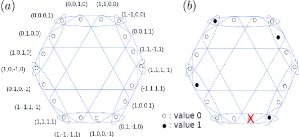
Figure 6.1: Each of the $18$ rays is depicted by a node, and the $9$ orthonormal bases are depicted by $9$ edges, each enclosing $4$ nodes. There is no KS-noncontextual assignment to these nodes. For instance, a noncontextual assignment of 0s and 1s to 17 of the nodes cannot be completed to an assignment to all 18 because neither 0 nor 1 can be assigned to the remaining node (marked X): one edge enclosing it requires it to be 0, the other 1.

Can the possibility of a KS-noncontextual ontological model be tested experimentally? One view is that it cannot, that the KS theorem merely constrains the possibilities for interpreting the quantum formalism [27, 66]. This answer, however, is inadequate. One can and should ask: what is the minimal set of operational predictions of quantum theory that need to be experimentally verified in order to show that it does not admit of a noncontextual model?

We show that this minimal set is a far cry from the whole of quantum theory and is therefore consistent with other possible operational theories such as the framework of generalized probabilistic theories [67, 68]. As such, our no-go result shows that none of these theories violating our noncontextuality inequality admits of a noncontextual model. Therefore, if corroborated by experiment, it implies that any future theory of physics that might replace quantum theory also fails to admit of a noncontextual model.

Let us briefly recall some definitions: An operational theory is a triple $(\mathcal{P},\mathcal{M},p)$ where $\mathcal{P}$ is a set of preparations, $\mathcal{M}$ is a set of measurements, and $p$ specifies, for every pair of preparation and measurement, the probability distribution over outcomes for that measurement if it is implemented on that preparation. Denoting the set of outcomes of measurement $M$ by $\mathcal{K}_{M}$, we have $\forall P\in\mathcal{P},\;\forall M\in\mathcal{M}$, $p(\cdot|P,M):\mathcal{K}_{M}\to[0,1]$.

An ontological model of an operational theory $(\mathcal{P},\mathcal{M},p)$ is a triple $(\Lambda,\mu,\xi)$, where $\Lambda$ denotes a space of possible ontic states for the physical system, $\mu$ specifies a probability distribution over the ontic states for every preparation procedure, that is, $\forall P\in\mathcal{P},\;\mu(\cdot|P):\Lambda\rightarrow[0,1]$, such that $\sum_{\lambda\in\Lambda}\mu(\lambda|P)=1$, and $\xi$ specifies, for every measurement, the conditional probability of obtaining a given outcome if the system is in a particular ontic state, that is, $\forall M\in\mathcal{M},\;\xi(k|M,\cdot):\Lambda\rightarrow[0,1]$, such that $\sum_{k\in\mathcal{K}_{M}}\xi(k|M,\lambda)=1$. The ontological model should reproduce the statistical predictions of the operational theory:

$$p(k|P,M)=\sum_{\lambda\in\Lambda}\xi(k|M,\lambda)\mu(\lambda|P)$$ (6.1)

for all $P\in\mathcal{P}$, and $M\in\mathcal{M}$.

We denote the event of obtaining outcome $k$ of measurement $M$ by $[k|M]$. If $[k|M]$ is assigned a deterministic outcome by every ontic state in the ontological model, i.e., if $\xi(k|M,\cdot):\Lambda\rightarrow\{0,1\}$, then it is said to be outcome-deterministic in that model.

6.2 Upgrading the Kochen-Specker theorem

We explain how to derive an experimental test of noncontextuality using a sequence of four refinements on the standard account of the KS theorem. In the first step, we identify the operational grounds that warrant applying an assumption of KS-noncontextuality to a measurement. In the second step, we explain why the assumption of outcome determinism for projective measurements – which is part of KS-noncontextuality – is unjustified, and in the third step, we show how it can be justified for a perfectly predictable measurement given an assumption of noncontextuality for preparations. In the fourth step, which is the central contribution of this chapter, we describe how to contend with the lack of perfect predictability that is characteristic of any real experiment.

6.2.1 Operationalizing the notion of KS-noncontextuality

In a KS-noncontextual model of operational quantum theory, the value (0 or 1) assigned to the event $[k|M]$ by $\lambda$ is the same as the value assigned to $[k^{\prime}|M^{\prime}]$ whenever these two events correspond to the same ray of Hilbert space (here, $M$ and $M^{\prime}$ are assumed to be maximal projective measurements). We get to the crux of KS-noncontextuality, therefore, by describing the operational grounds for associating the same ray to $[k|M]$ as is associated to $[k^{\prime}|M^{\prime}]$. Letting $\Pi_{k|M}$ and $\Pi_{k^{\prime}|M^{\prime}}$ represent the corresponding rank-1 projectors, the grounds for concluding that $\Pi_{k|M}=\Pi_{k^{\prime}|M^{\prime}}$ are that ${\rm tr}(\rho\Pi_{k|M})={\rm tr}(\rho\Pi_{k^{\prime}|M^{\prime}})$ for an appropriate set of density operators $\rho$. It is clearly sufficient for the equality to hold for the set of all density operators, but it is also sufficient to have equality for certain smaller sets of density operators, namely, those complete for measurement tomography.

What then should the operational grounds be for assigning the same value to $[k|M]$ and $[k^{\prime}|M^{\prime}]$ in a general operational theory, where preparations are not represented by density operators? The answer, clearly, is that the event $[k|M]$ occurs with the same probability as the event $[k^{\prime}|M^{\prime}]$ for all preparation procedures of the system,

$$p(k|M,P)=p(k^{\prime}|M^{\prime},P){\rm\;\;for\;all\;\;}P\in\mathcal{P},$$ (6.2)

or equivalently, if this holds for a subset of $\mathcal{P}$ that is tomographically complete. In this case, we shall say that $[k|M]$ and $[k^{\prime}|M^{\prime}]$ are operationally equivalent, and denote this as $[k|M]$ $\simeq$ $[k^{\prime}|M^{\prime}]$. We can therefore define a notion of KS-noncontextuality for any operational theory as follows: an ontological model $(\Lambda,\mu,\xi)$ of an operational theory $(\mathcal{P},\mathcal{M},p)$ is KS-noncontextual if (i) operational equivalence of events implies equivalent representations in the model, i.e., $[k|M]\simeq[k^{\prime}|M^{\prime}]\Rightarrow\xi(k|M,\lambda)=\xi(k^{\prime}|M^{\prime},\lambda)$ for all $\lambda\in\Lambda$, and (ii) the model is outcome-deterministic, $\xi(k|M,\cdot):\Lambda\to\{0,1\}.$

The operational equivalences among measurements required for the KS construction in Fig. 6.1(a) are made explicit in Fig. 6.2(a), where every measurement event $[k|M]$ is represented by a distinct node, and a novel type of edge between nodes specifies operational equivalence between events. This affords a nice depiction of contextual value assignments, as in Fig. 6.2(b). It follows that any operational theory with nine four-outcome measurements satisfying the operational equivalences depicted in Fig. 6.2(a) fails to admit of a KS-noncontextual model.

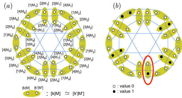
Figure 6.2: (a) Nine four-outcome measurements, each depicted by a set of four nodes encirled by a blue loop. A yellow hashed region enclosing a set of nodes implies that the corresponding events are operationally equivalent. (b) An illustration of the fact that there is no outcome-deterministic noncontextual assignment to the measurement events. The depicted outcome-deterministic assignment breaks the assumption of noncontextuality for the highlighted pair.

6.2.2 Defining noncontextuality without outcome determinism

The essence of noncontextuality is that context-independence at the operational level should imply context-independence at the ontological level. The operationalized version of KS-noncontextuality, however, makes an additional assumption about what sort of thing should be context-independent at the ontological level, namely, a deterministic assignment of an outcome. However, one can equally well assume that the ontic state merely assigns a probability distribution over outcomes, and take this distribution to be the thing that is context-independent. In Ref. [6], this revised notion of noncontextuality was termed measurement noncontextuality:

Measurement noncontextuality is satisfied by an ontological model $(\Lambda,\mu,\xi)$ of an operational theory $(\mathcal{P},\mathcal{M},p)$ if $[k|M]\simeq[k^{\prime}|M^{\prime}]$ implies $\xi(k|M,\lambda)=\xi(k^{\prime}|M^{\prime},\lambda)$ for all $\lambda\in\Lambda$.

Here, $\xi(k|M,\cdot)\in[0,1]$, so that outcome determinism is not assumed.

6.2.3 Justifying outcome determinism for perfectly predictable measurements

Outcome determinism can, however, be justified sometimes if one assumes a notion of noncontextuality for preparations [6]. First, a definition: $P$ and $P^{\prime}$ are said to be operationally equivalent, denoted $P\simeq P^{\prime}$, if for every measurement event $[k|M]$, $P$ assigns the same probability to this event as $P^{\prime}$ does, that is,

$$p(k|M,P)=p(k|M,P^{\prime}){\rm\;\;for\;all\;\;}k\in\mathcal{K}_{M},{\rm\;\;for\;all\;\;}M\in\mathcal{M}.$$ (6.3)

A preparation-noncontextual ontological model is then defined as follows:

Preparation noncontextuality is satisfied by an ontological model $(\Lambda,\mu,\xi)$ of an operational theory $(\mathcal{P},\mathcal{M},p)$ if $P\simeq P^{\prime}$ implies $\mu(\lambda|P)=\mu(\lambda|P^{\prime})$ for all $\lambda\in\Lambda$.

Insofar as both measurement and preparation noncontextuality are inferences from operational equivalence to ontological equivalence, it is most natural to assume both, that is, to assume universal noncontextuality.

As we showed in Chapter 1 (based on Ref. [6]), in a preparation-noncontextual model of quantum theory, all projective measurements must be represented outcome-deterministically. Here, we provide a version of this argument for the 18 ray construction.

Suppose that one has experimentally identified thirty-six preparation procedures organized into nine ensembles of four each, $\{P_{i,k}:i\in\{1,\dots,9\},k\in\{1,\dots,4\}\}$, such that for all $i$, measurement $M_{i}$ on preparation $P_{i,k}$ yields the $k$th outcome with certainty,

$$\forall i,\forall k:p(k|M_{i},P_{i,k})=1.$$ (6.4)

We call this property perfect predictability. In quantum theory, it suffices to let $P_{i,k}$ be the preparation associated with the pure state corresponding to the $k$th element of the $i$th measurement basis.

Figure 6.3: 36 preparation procedures, nine ensembles of four each. A node connected to the elements of an ensemble represents the effective preparation procedure achieved by sampling uniformly from the ensemble.

Define the effective preparation $P_{i}^{\rm(ave)}$ as the procedure obtained by sampling $k$ uniformly at random and then implementing $P_{i,k}$. Suppose one has experimentally verified the operational equivalences (Fig. 6.3)

$$P_{i}^{\rm(ave)}\simeq P_{i^{\prime}}^{\rm(ave)}{\rm\;\;for\;all\;}i,i^{\prime}\in\{1,\dots,9\}.$$ (6.5)

They hold in our quantum example because each $P_{i}^{\rm(ave)}$ corresponds to the completely mixed state.

Given Eq. (6.5) and the assumption of preparation noncontextuality, there is a single distribution over $\Lambda$, denoted $\nu(\lambda)$, such that

$$\mu(\lambda|P_{i}^{\rm(ave)})=\nu(\lambda){\rm\;\;for\;all\;}i\in\{1,\dots,9\}.$$ (6.6)

Given the definition of $P_{i}^{\rm(ave)}$, it follows that

$$\frac{1}{4}\sum_{k}\mu(\lambda|P_{i,k})=\nu(\lambda){\rm\;\;for\;all\;}i\in\{1,\dots,9\}.$$ (6.7)

Furthermore, recalling Eq. (6.1), for the ontological model to reproduce Eq. (6.4), we must have

$$\forall i,\forall k:\sum_{\lambda}\xi(k|M_{i},\lambda)\mu(\lambda|P_{i,k})=1.$$ (6.8)

Because every $\lambda$ in the support of $\nu(\lambda)$ appears in the support of $\mu(\lambda|P_{i,k})$ for some $k$, it follows that if $\xi(k|M_{i},\lambda)$ had an indeterministic response on any such $\lambda$, we would have a contradiction with Eq. (6.8). Consequently, for all $i$ and $k$, the measurement event $[k|M_{i}]$ must be outcome-deterministic for all $\lambda$ in the support of $\nu(\lambda)$.

To summarize then, if one has experimentally verified the operational equivalences depicted in Figs. 6.2(a) and 6.3 and the measurement statistics described in Eq. (6.4), then universal noncontextuality implies that the value assignments to measurement events should be deterministic and noncontextual, hence KS-noncontextual, and we obtain a contradiction:

$$\textrm{universal noncontextuality}\bigwedge\textrm{operational equivalences}$$

$$\bigwedge\textrm{perfect predictability}\Rightarrow\textrm{contradiction}.$$ (6.9)

6.2.4 Contending with imperfect predictability in real experiments

In real experiments, the ideal of perfect predictability described by Eq. (6.4) is never achieved, so we cannot derive a contradiction from it. However, Eq. (6.9) is logically equivalent to the following inference:

$$\textrm{universal noncontextuality}\bigwedge\textrm{operational equivalences}$$

$$\Rightarrow\textrm{failure of perfect predictability}.$$ (6.10)

That is, the degree of predictability, averaged over all $i$ and $k$, will necessarily be bounded away from 1. It is this bound that defines the operational noncontextuality inequality. For the 18 ray example, we prove that

$$A\equiv\frac{1}{36}\sum_{i=1}^{9}\sum_{k=1}^{4}p(k|M_{i},P_{i,k})\leq\frac{5}{6}.$$ (6.11)

We now outline how the bound in Eq. (6.11) is obtained. First, we use Eq. (6.1) to express $A$ in terms of $\xi(k|M_{i},\lambda)$ and $\mu(\lambda|P_{i,k})$. Defining the max-predictability of a measurement $M$ given an ontic state $\lambda$ by

$$\zeta(M,\lambda)\equiv\max_{k^{\prime}\in\mathcal{K}_{M}}\xi(k^{\prime}|M,\lambda),$$ (6.12)

we deduce that

$$A \leq \sum_{\lambda}\left(\frac{1}{9}\sum_{i}\zeta(M_{i},\lambda)\left[\frac{1}{4}\sum_{k}\mu(\lambda|P_{i,k})\right]\right)$$ (6.13)

$$= \sum_{\lambda}\left(\frac{1}{9}\sum_{i}\zeta(M_{i},\lambda)\right)\nu(\lambda)$$

$$\leq \max_{\lambda}\left(\frac{1}{9}\sum_{i}\zeta(M_{i},\lambda)\right),$$

where we have used Eq. (6.7).

The measurements can have indeterministic responses, $\xi(k|M,\cdot):\Lambda\rightarrow[0,1]$, but measurement noncontextuality implies that $\xi(k|M_{i},\lambda)=\xi(k^{\prime}|M_{i^{\prime}},\lambda)$ for the operationally equivalent pairs $\big{\{}[k|M_{i}],[k^{\prime}|M_{i^{\prime}}]\big{\}}$. There are many such assignments. Every unit-trace positive operator, for instance, specifies an indeterministic noncontextual assignment via the Born rule, and there are other, nonquantum assignments as well, such as the one depicted in Fig. 6.4.

Figure 6.4: A noncontextual outcome-indeterministic assignment

Consider the average max-predictability achieved by the assignment of Fig 6.4. Here, six measurements have max-predictability of 1, three of $\frac{1}{2}$, implying that $\frac{1}{9}\sum_{i}\zeta(M_{i},\lambda)=\frac{1}{9}(6\cdot 1+3\cdot\frac{1}{2})=\frac{5}{6}$. As we demonstrate in the formal proof of our noncontextuality inequality in the next section, no ontic state can do better, so that $\max_{\lambda}\left(\frac{1}{9}\sum_{i}\zeta(M_{i},\lambda)\right)\leq\frac{5}{6}$, thereby establishing the noncontextual bound on $A$. The logical limit for the value of $A$ is $1$, so the noncontextual bound of $\frac{5}{6}$ is nontrivial. The quantum realization of the 18 ray construction achieves $A=1$.

Following our formal proof of the inequality in the next section, we discuss the noise tolerance of our inequality, and we criticise a previous proposal for a noncontextuality inequality [70] on two main grounds: (i) that logic alone rules out the possiblity of satisfying it, and (ii) that all operational theories supporting the measurement equivalences of Fig. 6.2(a) necessarily violate it, regardless of whether or not they admit of a noncontextual model.

Although we have used the proof of Ref. [14] to illustrate our approach to deriving robust noncontextuality inequalities, our scheme can turn any proof of the Kochen-Specker theorem based on a KS-uncolourable set into an experimentally testable inequality, as we will show in the following section.

6.3 Proof of the inequality

Our noncontextuality inequality inspired by the proof of the Kochen-Specker theorem for the 18 ray KS-uncolourable set of Figure 6.1 can be summmarized by the following theorem:

Theorem 10.

Consider an operational theory $(\mathcal{P},\mathcal{M},p)$. Let $\{M_{i}\in\mathcal{M}:i\in\{1,\dots,9\}\}$ be nine four-outcome measurements. Let $[k|M_{i}]$ denote the $k$th outcome of the $i$th measurement, where $k\in\{1,\dots,4\}$. Let $\{P_{i,k}\in\mathcal{P}:i\in\{1,\dots,9\}$, $k\in\{1,2,3,4\}\}$ be thirty-six preparation procedures, organized into nine sets of four. Let $P^{\rm(ave)}_{i}\in\mathcal{P}$ be the preparation procedure obtained by sampling $k\in\{1,2,3,4\}$ uniformly at random and implementing $P_{i,k}$.

Suppose that one has experimentally verified the operational preparation equivalences depicted in Fig. 6.3, namely,

$$P^{\rm(ave)}_{1}\simeq P^{\rm(ave)}_{2}\simeq\dots\simeq P^{\rm(ave)}_{9},$$ (6.14)

and the operational equivalences depicted in Fig. 6.2(a), namely,

$$[k|M_{i}]\simeq[k^{\prime}|M_{i^{\prime}}],$$ (6.15)

for the eighteen pairs specifed therein.

If one assumes that the operational theory admits of a universally noncontextual ontological model, that is, one which is both measurement-noncontextual and preparation-noncontextual, then the following inequality on operational probabilities holds:

$$A\equiv\frac{1}{36}\sum_{i=1}^{9}\sum_{k=1}^{4}p(k|M_{i},P_{i,k})\leq\frac{5}{6}.$$ (6.16)

Figure 6.5: A choice of labelling of the eighteen equivalence classes of measurement events. Here, $w_{\kappa}$ denotes the probability assigned to the equivalence class labelled by $\kappa$ in a noncontextual outcome-indeterministic ontological model.

We now provide the proof. For clarity, we expand on some of the steps presented in previous section in our proof sketch.

The quantity $A$ can be expressed in terms of the distributions and response functions of the ontological model, using Eq. (6.1), as

$$A=\frac{1}{36}\sum_{i=1}^{9}\sum_{k=1}^{4}\sum_{\lambda}\xi(k|M_{i},\lambda)\mu(\lambda|P_{i,k}).$$ (6.17)

Using the definition of the max-probability $\zeta(M_{i},\lambda)$, given in Eq. (6.12), we have

$$A\leq\frac{1}{9}\sum_{i=1}^{9}\sum_{\lambda}\zeta(M_{i},\lambda)\left(\frac{1}{4}\sum_{k=1}^{4}\mu(\lambda|P_{i,k})\right).$$ (6.18)

Assuming that one experimentally verifies the operational preparation equivalences of Eq. (6.14), the assumption of preparation noncontextuality implies that

$$\mu(\lambda|P_{1}^{\rm(ave)})=\mu(\lambda|P_{2}^{\rm(ave)})=\cdots=\mu(\lambda|P_{9}^{\rm(ave)}).$$ (6.19)

It follows that there exists a single distribution, which we denote $\nu(\lambda)$, such that

$$\mu(\lambda|P_{i}^{\rm(ave)})=\nu(\lambda){\rm\;\;for\;all\;}i\in\{1,\dots,9\}.$$ (6.20)

Recall that $P_{i}^{\rm(ave)}$ is the preparation procedure that samples $k$ uniformly from $\{1,2,3,4\}$ and implements $P_{i,k}$. Given that the probability of the system being in a given ontic state $\lambda$ given the preparation $P_{i,k}$ is $\mu(\lambda|P_{i,k})$, and given that the probability of $P_{i,k}$ being implemented is $\frac{1}{4}$ for each value of $k$, it follows that the probability of the system being in a given ontic state $\lambda$ given the preparation $P_{i}^{\rm(ave)}$ is $\mu(\lambda|P_{i}^{\rm(ave)})=\frac{1}{4}\sum_{\lambda}\mu(\lambda|P_{i,k})$. Combining this with Eq. (6.20), we conclude that

$$\frac{1}{4}\sum_{\lambda}\mu(\lambda|P_{i,k})=\nu(\lambda){\rm\;\;for\;all\;}i\in\{1,\dots,9\},$$ (6.21)

and therefore that

$$A\leq\frac{1}{9}\sum_{\lambda}\sum_{i=1}^{9}\zeta(M_{i},\lambda)\nu(\lambda).$$ (6.22)

This in turn implies

$$A\leq\max_{\lambda}\frac{1}{9}\sum_{i=1}^{9}\zeta(M_{i},\lambda).$$ (6.23)

Assuming that one experimentally verifies the operational measurement equivalences of Eq. (6.15), the assumption of measurement noncontextuality implies that

$$\xi(k|M_{i},\lambda)=\xi(k^{\prime}|M_{i^{\prime}},\lambda),$$ (6.24)

for the eighteen pairs of operationally equivalent measurement events $([k|M_{i}],[k^{\prime}|M_{i^{\prime}}])$ specifed in Fig. 6.2(a).

It is useful to simplify the notation at this stage. We introduce the variable $\kappa\in\{1,\dots,18\}$ to range over the eighteen operational equivalence classes of measurement events. We introduce the shorthand notation

$$w_{\kappa}\equiv\xi(k|M_{i},\lambda)=\xi(k^{\prime}|M_{i^{\prime}},\lambda),$$ (6.25)

for the probability assigned to the $\kappa$th equivalence class, where the dependence on $\lambda$ is left implicit. The variable $\kappa$ enumerates the equivalence classes in Fig. 6.2(a), starting from $[1|M_{1}]$ and proceeding clockwise around the hypergraph, as depicted in Fig. 6.5.

In this notation, the constraint that each response function is probability-valued, $\xi(k|M_{i}.\lambda)\in[0,1]$, is simply

$$0\leq w_{\kappa}\leq 1,\;\;\forall\kappa\in\{1,\dots,18\},$$ (6.26)

while the constraint that the set of response functions for each measurement sum to 1, $\sum_{k=1}^{4}\xi(k|M_{i},\lambda)=1$, can be captured by the matrix equality

$$Z\vec{w}=\vec{u}$$ (6.27)

where $\vec{w}\equiv(w_{1},\dots,w_{18})^{T}$, $\vec{u}\equiv(1,1,1,1,1,1,1,1,1)^{T}$, and

$$Z\equiv\left(\begin{array}[]{cccccccccccccccccc}1&1&1&1&0&0&0&0&0&0&0&0&0&0&0&0&0&0\\ 0&0&0&1&1&1&1&0&0&0&0&0&0&0&0&0&0&0\\ 0&0&0&0&0&0&1&1&1&1&0&0&0&0&0&0&0&0\\ 0&0&0&0&0&0&0&0&0&1&1&1&1&0&0&0&0&0\\ 0&0&0&0&0&0&0&0&0&0&0&0&1&1&1&1&0&0\\ 1&0&0&0&0&0&0&0&0&0&0&0&0&0&0&1&1&1\\ 0&1&0&0&0&0&0&0&1&0&1&0&0&0&0&0&0&1\\ 0&0&1&0&1&0&0&0&0&0&0&1&0&1&0&0&0&0\\ 0&0&0&0&0&1&0&1&0&0&0&0&0&0&1&0&1&0\end{array}\right).$$ (6.28)

Finally, we can express the quantity to be maximized as

$$\frac{1}{9}\sum_{i=1}^{9}\zeta(M_{i},\lambda)=\frac{1}{9}\sum_{i=1}^{9}\max_{\kappa:Z_{i\kappa}=1}w_{\kappa},$$ (6.29)

or, more explicitly, as

$$\frac{1}{9}\sum_{i=1}^{9}\zeta(M_{i},\lambda)$$

$$=\frac{1}{9}[\max\{w_{1},w_{2},w_{3},w_{4}\}+\max\{w_{4},w_{5},w_{6},w_{7}\}$$

$$+\max\{w_{7},w_{8},w_{9},w_{10}\}+\max\{w_{10},w_{11},w_{12},w_{13}\}$$

$$+\max\{w_{13},w_{14},w_{15},w_{16}\}+\max\{w_{16},w_{17},w_{18},w_{1}\}$$

$$+\max\{w_{18},w_{2},w_{9},w_{11}\}+\max\{w_{3},w_{5},w_{12},w_{14}\}$$

$$+\max\{w_{6},w_{8},w_{15},w_{17}\}].$$ (6.30)

The matrix equality of Eq. (6.27) implies that there are only nine independent variables in the set $\{w_{1},w_{2},\dots,w_{18}\}$ and that these satisfy linear inequalities. The space of possibilities for the vector $\vec{w}$ therefore forms a nine-dimensional polytope in the hypercube described by Eq. (6.23).

The value of $\frac{1}{9}\sum_{i=1}^{9}\zeta(M_{i},\lambda)$ on any of the interior points of this polytope will be an average of its values at the vertices because it is a convex function of $\vec{w}$. Therefore, to implement the maximization over $\lambda$, it suffices to maximize over the vertices of this polytope.

Using the numerical software Sage, in particular the Polyhedron class in SageMathCloud[74], we were able to infer all 146 vertices of our 9-dimensional polytope from its characterization in terms of the linear inequalities obtained from Eqs. (6.26) and (6.27). From this brute-force enumeration of all the vertices of the polytope, the maximum possible value of $\frac{1}{9}\sum_{i=1}^{9}\zeta(M_{i},\lambda)$ was found to be $\frac{5}{6}$. An example of a vertex achieving this value is $\vec{w}=(1,0,0,0,1,0,0,0,\tfrac{1}{2},\tfrac{1}{2},\tfrac{1}{2},0,0,0,1,0,0,0)^{\rm T}$, which is depicted in Fig. 6.4. This concludes the proof.

Our proof technique can be adapted to derive a similar noncontextuality inequality correponding to any proof of the KS theorem based on the KS-uncolourability of a set of rays of Hilbert space. One begins by completing every set of orthogonal rays into a basis of the Hilbert space, and then forming the hypergraph depicting the orthogonality relations among these rays (the analogue of Fig. 6.1). One then forms the hypergraph depicting all of the measurements events, with one type of edge denoting which events correspond to the outcomes of a single measurement, and the other type of edge denoting when a set of measurement events are operationally equivalent (the analogue of Fig. 6.2(a)). One then associates a set of preparations with every measurement in the hypergraph, one preparation for every outcome. For each such set of preparations, we define the effective preparation that is the uniform mixture of the set’s elements, and we presume that all of the effective preparations so defined are operationally equivalent (as is the case in quantum theory, where the effective preparation for every set corresponds to the completely mixed state). We consider the correlation between the measurement outcome and the choice of preparation in the set associated with that measurement, averaged over all measurements. This average correlation is the quantity $A$ that appears on the left-hand side of the operational noncontextuality inequality.

The KS-uncolourability of the hypergraph means that there are no noncontextual deterministic assignments to the measurement events, hence the polytope of probabilistic assignments to the measurement events has no deterministic vertices either. Each vertex of this polytope, that is, each convexly-extremal probabilistic assignment, will necessarily yield an indeterministic assignment to some of the measurement events. Using the operational equivalences and the assumption of universal noncontextuality, one can infer from this that the average correlation $A$ is always bounded away from 1. For any KS-uncolourable hypergraph, a quantum realization would achieve the logical limit $A=1$ by construction, so the noncontextuality inequality we derive is necessarily violated by quantum theory in each case. The exact upper bound on $A$ will depend on the vertices of the polytope of measurement noncontextual probability assignments possible on the KS-uncolourable hypergraph and will therefore vary from case to case (but will always be less than 1).

One can understand this violation as being due to the fact that assignments of density operators that are independent of the preparation context can achieve higher predictability for the respective measurements than assignments of probability distributions over ontic states that are independent of the preparation context. This is the feature of quantum theory that allows it to maximally violate the noncontextual bound of $A\leq 5/6$.

6.4 Vertices of the polytope

In this section, we describe the vertices of the polytope of possible probabilistic assignments to the $18$ equivalence classes of measurement events in the hypergraph of Fig. 6.5. These vertices correspond to the convexly-extremal probabilistic assignments. Since we use these vertices in proving our noncontextuality inequality, we discuss some of their characteristics below.

6.4.1 Odd n-cycles in the hypergraph

We begin by noting a property of the hypergraph of Fig. 6.5, namely, the presence of odd $n$-cycles. An odd $n$-cycle of equivalence classes of measurement events is an ordered sequence of $n$ such classes wherein adjacent elements in the sequence contain measurement events that are distinct outcomes of a single measurement. For instance, the sequence of equivalence classes $(1,2,18)$ in Fig. 6.5 forms a $3$-cycle because for the first adjacent pair in the sequence, $(1,2)$, there is a node within the class 1 and a node within the class 2 that appear together in the same edge, and similarly for the two other adjacent pairs, $(2,18)$, and $(18,1)$.

We note the presence of the following odd $n$-cycles in Fig. 6.5 which will be of interest further on:

1. $3$-cycle: $(1,2,18)$

2. $5$-cycle: $(8,9,11,13,15)$

3. $7$-cycle: $(1,3,5,7,10,11,18)$

4. $9$-cycle: $(1,4,6,15,14,12,10,9,18)$

6.4.2 Quantum probabilistic assignments: the projective and the nonprojective cases

A given probabilistic assignment $\{w_{\kappa}\}_{\kappa=1}^{18}$ is quantum-realizable if one can associate an effect $E_{\kappa}$—that is, a positive operator less than identity, $0\leq E_{\kappa}\leq I$—to each node $\kappa$, such that each of the edges of the hypergraph correspond to positive operator-valued measures, $\sum_{\kappa\in{\rm edge}}E_{\kappa}=I$, and one can find a unit-trace positive operator $\rho$ such that $w_{\kappa}={\rm tr}(E_{\kappa}\rho)$. In other words a given probabilistic assignment to the measurements is quantum-realizable if there is a set of quantum measurements and a quantum state that yield this probabilistic assignment via the Born rule. Such quantum realizability of probabilistic assignments when the POVMs are restricted to projective measurements is the question of interest in the traditional Kochen-Specker type approach to contextuality, most recently exemplified in the work of Refs. [25] and [26]. In our approach, this question is not the one of interest, particularly because even if we restrict ourselves to quantum theory, we want to be able to deal with all POVMs – projective or nonprojective – on an equal footing without having to artificially constrain ourselves to just projective measurements. However, we will still study this question so that the distinction between the traditional approach [26, 25] and our approach becomes clearer.

As we will show, none of the vertices of the polytope of probabilistic assignments (Fig. 6.5) on the KS-uncolourable hypergraph of Fig. 6.1(a) is quantum realizable via projectors. That is, considering every assignment of projectors to nodes of the hypergraph (such that projectors in an edge of the hypergraph sum to identity) and every quantum state, the probabilistic assignment that results is never a vertex of the polytope. Consider, for example, the extremal probabilistic assignment to the equivalence classes in Fig. 6.4: this requires the assignment $w_{1}=w_{2}=w_{18}=1/2$ to the $3$-cycle $(1,2,18)$. If the experiment is modelled by the quantum formalism, then because joint measurability is represented by orthogonality of projectors, any odd $n$-cycle must be represented by a sequence of projectors that are orthogonal for contiguous pairs. Any odd $n$-cycle with such assignments ($w_{\kappa}=1/2$ for all $\kappa$ in the odd $n$-cycle) does not admit a realization with projectors as the following lemma shows:

Lemma 4.

Given a set of $n$ projectors (where $n$ is odd), $\{\Pi_{1},\Pi_{2},\dots,\Pi_{n}\}$, satisfying orthogonality between adjacent pairs, $\Pi_{i}\Pi_{i\oplus 1}=0$ for all $i\in\{1,2,\dots,n\}$ (we call this set of projectors an odd $n$-cycle), there exists no quantum state $\rho$, $\rho\geq 0$ and ${\rm Tr}\rho=1$, such that

$$\forall i\in\{1,2,\dots,n\}:\text{Tr}(\rho\Pi_{i})=\frac{1}{2}.$$ (6.31)

Proof. This follows from noting that Eq. (6.31) implies $\forall i\in\{1,2,\dots,n\}$: $\text{Tr}\left(\rho(\Pi_{i}+\Pi_{i\oplus 1})\right)=1$. Since $\Pi_{i}$ and $\Pi_{i\oplus 1}$ are orthogonal, we have $\Pi_{i}+\Pi_{i\oplus 1}\leq I$ for all $i$. We also have $\Pi_{i}+\Pi_{i}^{\perp}=I$ for all $i$, where $\Pi_{i}^{\perp}$ is the projector onto the subspace orthogonal to $\Pi_{i}$. Hence, we must have $\Pi_{i\oplus 1}\leq\Pi_{i}^{\perp}$, but since we are given $\text{Tr}(\rho\Pi_{i\oplus 1})=\frac{1}{2}$ and can infer $\text{Tr}(\rho\Pi_{i}^{\perp})=\frac{1}{2}$ (because $\text{Tr}(\rho\Pi_{i})=\frac{1}{2}$), we in fact have $\Pi_{i\oplus 1}=\Pi_{i}^{\perp}$ for all $i$. When $n$ is odd, this means that the list of projectors reads as $\{\Pi_{1}=\Pi_{n}^{\perp},\Pi_{2}=\Pi_{1}^{\perp},\Pi_{3}=\Pi_{2}^{\perp}=\Pi_{1},\Pi_{4}=\Pi_{1}^{\perp},\dots,\Pi_{n}=\Pi_{1}\}$, leading to the contradiction $\Pi_{1}=\Pi_{1}^{\perp}$ (impossible because $\Pi_{1}$ is a projector). Hence such a valuation as in Eq. (6.31) is impossible in quantum theory with projectors for any quantum state $\rho$.

It follows from this lemma that $3$-cycle correlations of this form are not realizable via quantum projectors. These correspond to the indeterministic extremal points of the polytope of correlations in Specker’s scenario we discussed in Chapter 5 (see also Ref. [58]), in particular the “overprotective seer” correlations of Ref. [29].

More generally, we can use Lemma 4 to argue that none of the vertices admit a quantum realization with projectors. This is because every vertex involves an odd $n$-cycle with probabilities $1/2$ assigned to nodes in that $n$-cycle. On the other hand, any vertex with assignments $\{w_{\kappa}\}_{\kappa=1}^{18}$ can always be realized quantumly by assigning trivial effects of the form $w_{\kappa}I$ to each node labelled by $\kappa\in\{1,2,\dots,18\}$, where $I$ denotes the identity operator. However, such trivial quantum realizations are indeed trivial: they do not admit contextuality in our approach because they are too noisy to ever achieve $A>5/6$, as we will show in the next section on the noise robustness of our inequality. In fact, something stronger can be said: the trivial effect assignments, $\{w_{\kappa}I\}_{\kappa=1}^{18}$, corresponding to any point belonging to the polytope (including the vertices of the polytope) achieve $A=1/4$, which is way below the noncontextual upper bound of $5/6$. This is easy to see: the statistics of $w_{\kappa}I$, given the Born rule, is independent of what preparation (density operator) precedes such a “measurement” outcome, so we have $p(k|M_{i},P_{i,k})=\text{Tr}(\rho_{i,k}w_{\kappa}I)=w_{\kappa}$, independent of the density operator $\rho_{i,k}$ that may be associated with preparation $P_{i,k}$. A trivial quantum realization, therefore, achieves $\sum_{k=1}^{4}p(k|M_{i},P_{i,k})=1$ for each $i\in\{1,2,\dots,9\}$, and we have $A=\frac{1}{36}(9)=1/4$. (Note that for a projective quantum realization we can have $\sum_{k=1}^{4}p(k|M_{i},P_{i,k})=4$ for each $i$ and therefore $A=1$.)

Hence, all such trivial quantum realizations (and not only those of the vertices) are on the same footing so far as our noncontextuality inequality is concerned. The operational significance of this should be clear: in order to even approach the noncontextual upper bound of our inequality, one needs to have some projective component to the quantum measurements; they can’t all be so noisy that they are rendered trivial.

Thus our noncontextuality inequality clarifies the precise sense in which such assignments are trivial, something which is never clear in the traditional Kochen-Specker approach to noncontextuality where the vertices of the polytope could be naively deemed “maximally (KS)contextual”, and the fact that they admit trivial quantum realizations of this sort is ignored by restricting attention to sharp (projective) measurements (see, for example, Refs. [25, 26]).

6.4.3 Classification of the vertices

Classified in terms of their average predictability, $\frac{1}{9}\sum_{i=1}^{9}\zeta(M_{i},\lambda)$, the $146$ vertices of the $9$-dimensional polytope fall into four types, depicted in Table 6.1. Each row of the table corresponds to a particular type. The first column labels the type of vertex; the second column notes the average predictability of vertices of this type; the third column describes an example vertex of the given type; the fourth column specifies, for the given example, the particular $n$-cycle that makes it impossible on account of Lemma 4 to build a (projective) quantum realization of that vertex, and notes the value of $n$ which makes a projective quantum realization impossible for all vertices of that type; the last column notes the number of instances of the given type of vertex in the set of 146 vertices. See Tables 6.2, 6.3, 6.4, and 6.5 for the complete list of all the four types of vertices.

Type of vertex	$\frac{1}{9}\sum_{i=1}^{9}\zeta(M_{i},\lambda)$	Example vertex	$n$-cycle excluding projective realization (Lemma 4)	Number of vertices
$1$	$\frac{1}{9}(6+3\frac{1}{2})=5/6$	See figure 6.6	$(1,2,18)$, $n=3$	24
$2$	$\frac{1}{9}(4+5\frac{1}{2})=13/18$	See figure 6.7	$(8,9,11,13,15)$, $n=5$	$36$
$3$	$\frac{1}{9}(2+7\frac{1}{2})=11/18$	See figure 6.8	$(1,3,5,7,10,11,18)$, $n=7$	$36$
$4$	$\frac{1}{9}(0+9\frac{1}{2})=1/2$	See figure 6.9	$(1,4,6,15,14,12,10,9,18)$, $n=9$	$50$

Table 6.1: Classification of the $146$ vertices of the $9$-dimensional polytope of probabilistic assignments to nodes of the hypergraph of Fig. 6.5.

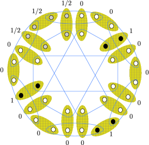
Figure 6.6: An example of a vertex of type $1$.

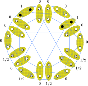
Figure 6.7: An example of a vertex of type $2$.

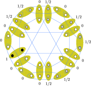
Figure 6.8: An example of a vertex of type $3$.

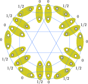
Figure 6.9: An example of a vertex of type $4$.

$w_{1}$	$w_{2}$	$w_{3}$	$w_{4}$	$w_{5}$	$w_{6}$	$w_{7}$	$w_{8}$	$w_{9}$	$w_{10}$	$w_{11}$	$w_{12}$	$w_{13}$	$w_{14}$	$w_{15}$	$w_{16}$	$w_{17}$	$w_{18}$
1/2	1/2	0	0	1	0	0	0	0	1	0	0	0	0	1	0	0	1/2
1/2	1/2	0	0	0	0	1	0	0	0	0	1	0	0	1	0	0	1/2
1/2	1/2	0	0	0	1	0	0	0	1	0	0	0	1	0	0	0	1/2
1/2	1/2	0	0	1	0	0	1	0	0	0	0	1	0	0	0	0	1/2
0	0	1/2	1/2	1/2	0	0	0	0	1	0	0	0	0	1	0	0	1
0	0	1/2	1/2	1/2	0	0	1	0	0	0	0	1	0	0	0	0	1
0	0	1/2	1/2	1/2	0	0	0	1	0	0	0	1	0	0	0	1	0
0	0	1/2	1/2	1/2	0	0	1	0	0	1	0	0	0	0	1	0	0
0	0	1	0	0	1/2	1/2	1/2	0	0	0	0	1	0	0	0	0	1
1	0	0	0	0	1/2	1/2	1/2	0	0	1	0	0	1	0	0	0	0
0	1	0	0	0	1/2	1/2	1/2	0	0	0	1	0	0	0	1	0	0
0	0	1	0	0	1/2	1/2	1/2	0	0	1	0	0	0	0	1	0	0
1	0	0	0	1	0	0	0	1/2	1/2	1/2	0	0	0	1	0	0	0
1	0	0	0	0	1	0	0	1/2	1/2	1/2	0	0	1	0	0	0	0
0	0	0	1	0	0	0	0	1/2	1/2	1/2	0	0	1	0	0	1	0
0	0	1	0	0	1	0	0	1/2	1/2	1/2	0	0	0	0	1	0	0
0	0	0	1	0	0	0	1	0	0	0	1/2	1/2	1/2	0	0	0	1
0	0	0	1	0	0	0	0	1	0	0	1/2	1/2	1/2	0	0	1	0
0	1	0	0	0	0	1	0	0	0	0	1/2	1/2	1/2	0	0	1	0
1	0	0	0	0	1	0	0	1	0	0	1/2	1/2	1/2	0	0	0	0
0	1	0	0	0	0	1	0	0	0	0	1	0	0	1/2	1/2	1/2	0
0	1	0	0	1	0	0	0	0	1	0	0	0	0	1/2	1/2	1/2	0
0	0	0	1	0	0	0	0	1	0	0	1	0	0	1/2	1/2	1/2	0
0	0	1	0	0	0	1	0	0	0	1	0	0	0	1/2	1/2	1/2	0

Table 6.2: The $24$ vertices of Type 1.

$w_{1}$	$w_{2}$	$w_{3}$	$w_{4}$	$w_{5}$	$w_{6}$	$w_{7}$	$w_{8}$	$w_{9}$	$w_{10}$	$w_{11}$	$w_{12}$	$w_{13}$	$w_{14}$	$w_{15}$	$w_{16}$	$w_{17}$	$w_{18}$
1	0	0	0	1	0	0	1/2	1/2	0	1/2	0	1/2	0	1/2	0	0	0
1	0	0	0	1/2	0	1/2	0	1/2	0	1/2	1/2	0	0	1	0	0	0
1	0	0	0	1/2	1/2	0	0	1	0	0	1/2	1/2	0	1/2	0	0	0
1	0	0	0	1/2	0	1/2	1/2	0	0	1	0	0	1/2	1/2	0	0	0
1	0	0	0	1/2	0	1/2	0	1/2	0	1/2	1/2	0	0	1	0	0	0
0	1	0	0	1/2	0	1/2	0	0	1/2	0	0	1/2	1/2	0	0	1	0
0	1	0	0	1/2	1/2	0	1/2	0	1/2	0	1/2	0	0	0	1	0	0
0	1	0	0	1/2	1/2	0	0	0	1	0	0	0	1/2	0	1/2	1/2	0
0	1	0	0	1	0	0	1/2	0	1/2	0	0	1/2	0	0	1/2	1/2	0
0	0	1	0	0	1	0	0	1/2	1/2	0	0	1/2	0	0	1/2	0	1/2
0	0	1	0	0	1/2	1/2	0	1/2	0	0	0	1	0	0	0	1/2	1/2
0	0	1	0	0	1/2	1/2	0	0	1/2	0	0	1/2	0	1/2	0	0	1
0	0	1	0	0	0	1	0	0	0	1/2	0	1/2	0	1/2	0	1/2	1/2
0	0	0	1	0	0	0	1/2	1/2	0	0	1	0	0	1/2	1/2	0	1/2
0	0	0	1	0	0	0	1/2	0	1/2	1/2	0	0	1	0	0	1/2	1/2
0	0	0	1	0	0	0	1/2	0	1/2	0	1/2	0	1/2	1/2	0	0	1
0	0	0	1	0	0	0	1	0	0	1/2	1/2	0	1/2	0	1/2	0	1/2
0	0	1/2	1/2	0	0	1/2	0	0	1/2	0	1/2	0	0	1	0	0	1
0	0	1/2	1/2	0	1/2	0	0	0	1	0	0	0	1/2	1/2	0	0	1
0	1/2	0	1/2	0	0	1/2	0	0	1/2	1/2	0	0	1	0	0	1	0
0	1/2	0	1/2	0	1/2	0	0	0	1	0	0	0	1	0	0	1/2	1/2
0	1/2	0	1/2	0	1/2	0	1/2	1/2	0	0	1	0	0	0	1	0	0
0	1/2	0	1/2	1/2	0	0	1	0	0	1/2	1/2	0	0	0	1	0	0
0	1/2	1/2	0	0	0	1	0	0	0	1/2	0	1/2	1/2	0	0	1	0
0	1/2	1/2	0	1/2	0	1/2	0	1/2	0	0	0	1	0	0	0	1	0
0	1/2	1/2	0	0	1	0	0	0	1	0	0	0	1/2	0	1/2	0	1/2
0	1/2	1/2	0	0	1	0	0	1/2	1/2	0	1/2	0	0	0	1	0	0
1/2	0	0	1/2	0	0	1/2	0	1/2	0	0	1	0	0	1	0	0	1/2
1/2	0	0	1/2	0	0	1/2	1/2	0	0	1	0	0	1	0	0	1/2	0
1/2	0	0	1/2	0	1/2	0	0	1	0	0	1	0	0	1/2	1/2	0	0
1/2	0	0	1/2	1/2	0	0	1	0	0	1	0	0	1/2	0	1/2	0	0
1/2	0	1/2	0	1/2	1/2	0	0	1	0	0	0	1	0	0	0	1/2	0
1/2	0	1/2	0	0	1	0	0	1	0	0	1/2	1/2	0	0	1/2	0	0
1/2	0	1/2	0	0	0	1	0	0	0	1	0	0	1/2	1/2	0	1/2	0
1/2	0	1/2	0	0	0	1	0	0	0	1/2	1/2	0	0	1	0	0	1/2
1/2	1/2	0	0	1	0	0	1/2	1/2	0	0	0	1	0	0	0	1/2	0
1/2	1/2	0	0	1	0	0	1	0	0	1/2	0	1/2	0	0	1/2	0	0

Table 6.3: The $36$ vertices of Type 2.

$w_{1}$	$w_{2}$	$w_{3}$	$w_{4}$	$w_{5}$	$w_{6}$	$w_{7}$	$w_{8}$	$w_{9}$	$w_{10}$	$w_{11}$	$w_{12}$	$w_{13}$	$w_{14}$	$w_{15}$	$w_{16}$	$w_{17}$	$w_{18}$
1/2	0	1/2	0	1/2	0	1/2	0	0	1/2	1/2	0	0	0	1	0	0	1/2
1/2	0	1/2	0	1/2	1/2	0	1/2	1/2	0	0	0	1	0	0	0	0	1/2
1/2	0	1/2	0	0	1	0	0	1/2	1/2	0	0	1/2	1/2	0	0	0	1/2
1/2	0	1/2	0	1/2	0	1/2	1/2	0	0	1	0	0	0	1/2	1/2	0	0
1/2	0	0	1/2	1/2	0	0	0	1/2	1/2	0	1/2	0	0	1	0	0	1/2
1/2	0	0	1/2	0	1/2	0	1/2	0	1/2	1/2	0	0	1	0	0	0	1/2
1/2	0	0	1/2	1/2	0	0	1	0	0	1/2	0	1/2	1/2	0	0	0	1/2
1/2	0	0	1/2	1/2	0	0	0	1	0	0	1/2	1/2	0	1/2	0	1/2	0
0	0	1/2	1/2	0	1/2	0	1/2	0	1/2	0	0	1/2	1/2	0	0	0	1
0	0	1/2	1/2	0	0	1/2	0	1/2	0	1/2	0	1/2	1/2	0	0	1	0
0	0	1/2	1/2	0	0	1/2	1/2	0	0	0	1/2	1/2	0	1/2	0	0	1
0	0	1/2	1/2	0	1/2	0	0	1	0	0	1/2	1/2	0	0	1/2	1/2	0
0	0	1/2	1/2	0	0	1/2	1/2	0	0	1	0	0	1/2	0	1/2	1/2	0
0	0	1/2	1/2	0	1/2	0	1/2	1/2	0	1/2	1/2	0	0	0	1	0	0
0	1/2	0	1/2	1/2	0	0	0	1/2	1/2	0	0	1/2	1/2	0	0	1	0
0	1/2	0	1/2	1/2	0	0	1	0	0	0	1/2	1/2	0	0	1/2	0	1/2
0	1/2	0	1/2	0	0	1/2	1/2	0	0	0	1	0	0	1/2	1/2	0	1/2
0	1/2	0	1/2	1/2	0	0	0	0	1	0	0	0	1/2	1/2	0	1/2	1/2
1/2	1/2	0	0	0	1/2	1/2	0	0	1/2	1/2	0	0	1	0	0	1/2	0
1/2	1/2	0	0	0	1	0	0	1/2	1/2	0	1/2	0	1/2	0	1/2	0	0
1/2	1/2	0	0	1	0	0	1/2	0	1/2	1/2	0	0	0	1/2	1/2	0	0
1/2	1/2	0	0	1	0	0	0	1/2	1/2	0	0	1/2	0	1/2	0	1/2	0
1/2	1/2	0	0	0	0	1	0	0	0	1/2	1/2	0	1/2	1/2	0	1/2	0
1/2	1/2	0	0	0	1/2	1/2	0	1/2	0	0	1	0	0	1/2	1/2	0	0
0	1/2	1/2	0	1/2	0	1/2	1/2	0	0	0	0	1	0	0	0	1/2	1/2
0	1/2	1/2	0	1/2	1/2	0	0	0	1	0	0	0	0	1/2	1/2	0	1/2
0	1/2	1/2	0	1/2	1/2	0	1/2	0	1/2	1/2	0	0	0	0	1	0	0
0	1/2	1/2	0	0	0	1	0	0	0	0	1/2	1/2	0	1/2	0	1/2	1/2
1	0	0	0	1/2	1/2	0	1/2	1/2	0	1/2	0	1/2	1/2	0	0	0	0
1	0	0	0	0	1/2	1/2	0	1/2	0	1/2	1/2	0	1/2	1/2	0	0	0
0	1	0	0	0	1/2	1/2	0	0	1/2	0	1/2	0	1/2	0	1/2	1/2	0
0	1	0	0	1/2	0	1/2	1/2	0	0	0	1/2	1/2	0	0	1/2	1/2	0
0	0	1	0	0	1/2	1/2	0	1/2	0	1/2	0	1/2	0	0	1/2	1/2	0
0	0	1	0	0	1/2	1/2	0	0	1/2	1/2	0	0	0	1/2	1/2	0	1/2
0	0	0	1	0	0	0	0	1/2	1/2	0	1/2	0	1/2	1/2	0	1/2	1/2
0	0	0	1	0	0	0	1/2	1/2	0	1/2	1/2	0	1/2	0	1/2	1/2	0

Table 6.4: The $36$ vertices of Type 3.

$w_{1}$	$w_{2}$	$w_{3}$	$w_{4}$	$w_{5}$	$w_{6}$	$w_{7}$	$w_{8}$	$w_{9}$	$w_{10}$	$w_{11}$	$w_{12}$	$w_{13}$	$w_{14}$	$w_{15}$	$w_{16}$	$w_{17}$	$w_{18}$
1/2	0	0	1/2	0	1/2	0	0	1/2	1/2	0	1/2	0	1/2	1/2	0	0	1/2
1/2	0	0	1/2	1/2	0	0	1/2	1/2	0	1/2	1/2	0	0	1/2	1/2	0	0
1/2	0	0	1/2	0	1/2	0	1/2	1/2	0	1/2	1/2	0	1/2	0	1/2	0	0
1/2	0	0	1/2	0	0	1/2	0	1/2	0	1/2	1/2	0	1/2	1/2	0	1/2	0
1/2	0	0	1/2	0	0	1/2	1/2	0	0	1/2	1/2	0	1/2	1/2	0	0	1/2
1/2	0	0	1/2	1/2	0	0	1/2	0	1/2	1/2	0	0	1/2	1/2	0	0	1/2
1/2	0	0	1/2	1/2	0	0	1/2	1/2	0	1/2	0	1/2	1/2	0	0	1/2	0
1/2	0	0	1/2	1/2	0	0	1/2	1/2	0	0	1/2	1/2	0	1/2	0	0	1/2
0	0	1/2	1/2	0	1/2	0	0	1/2	1/2	0	1/2	0	0	1/2	1/2	0	1/2
0	0	1/2	1/2	0	1/2	0	1/2	1/2	0	0	1/2	1/2	0	0	1/2	0	1/2
0	0	1/2	1/2	1/2	0	0	0	1/2	1/2	1/2	0	0	0	1/2	1/2	1/2	0
0	0	1/2	1/2	0	1/2	0	1/2	0	1/2	1/2	0	0	1/2	0	1/2	0	1/2
0	0	1/2	1/2	0	0	1/2	1/2	0	0	1/2	1/2	0	0	1/2	1/2	0	1/2
0	0	1/2	1/2	0	1/2	0	0	1/2	1/2	0	0	1/2	1/2	0	0	1/2	1/2
0	0	1/2	1/2	0	0	1/2	0	0	1/2	1/2	0	0	1/2	1/2	0	1/2	1/2
0	0	1/2	1/2	0	0	1/2	0	1/2	0	0	1/2	1/2	0	1/2	0	1/2	1/2
0	0	1/2	1/2	0	0	1/2	1/2	0	0	1/2	0	1/2	1/2	0	0	1/2	1/2
0	1/2	0	1/2	1/2	0	0	1/2	1/2	0	0	1/2	1/2	0	0	1/2	1/2	0
0	1/2	0	1/2	0	1/2	0	0	1/2	1/2	0	1/2	0	1/2	0	1/2	1/2	0
0	1/2	0	1/2	1/2	0	0	1/2	0	1/2	1/2	0	0	1/2	0	1/2	1/2	0
0	1/2	0	1/2	1/2	0	0	1/2	0	1/2	0	1/2	0	0	1/2	1/2	0	1/2
0	1/2	0	1/2	0	0	1/2	1/2	0	0	1/2	1/2	0	1/2	0	1/2	1/2	0
0	1/2	0	1/2	0	1/2	0	1/2	0	1/2	0	1/2	0	1/2	0	1/2	0	1/2
0	1/2	0	1/2	1/2	0	0	1/2	0	1/2	0	0	1/2	1/2	0	0	1/2	1/2
0	1/2	0	1/2	0	0	1/2	0	0	1/2	0	1/2	0	1/2	1/2	0	1/2	1/2
0	1/2	1/2	0	1/2	1/2	0	0	1/2	1/2	0	0	1/2	0	0	1/2	1/2	0
0	1/2	1/2	0	0	1/2	1/2	0	0	1/2	0	1/2	0	0	1/2	1/2	0	1/2
0	1/2	1/2	0	1/2	0	1/2	1/2	0	0	1/2	0	1/2	0	0	1/2	1/2	0
0	1/2	1/2	0	0	1/2	1/2	0	0	1/2	1/2	0	0	1/2	0	1/2	1/2	0
0	1/2	1/2	0	0	1/2	1/2	0	1/2	0	0	1/2	1/2	0	0	1/2	1/2	0
0	1/2	1/2	0	1/2	1/2	0	1/2	0	1/2	0	0	1/2	0	0	1/2	0	1/2
0	1/2	1/2	0	1/2	0	1/2	0	0	1/2	0	0	1/2	0	1/2	0	1/2	1/2
0	1/2	1/2	0	0	1/2	1/2	0	0	1/2	0	0	1/2	1/2	0	0	1/2	1/2
1/2	1/2	0	0	1/2	0	1/2	1/2	0	0	1/2	1/2	0	0	1/2	1/2	0	0
1/2	1/2	0	0	1/2	1/2	0	1/2	0	1/2	1/2	0	0	1/2	0	1/2	0	0
1/2	1/2	0	0	1/2	1/2	0	1/2	1/2	0	0	1/2	1/2	0	0	1/2	0	0
1/2	1/2	0	0	1/2	1/2	0	0	1/2	1/2	0	1/2	0	0	1/2	1/2	0	0
1/2	1/2	0	0	0	1/2	1/2	1/2	0	0	0	1/2	1/2	1/2	0	0	0	1/2
1/2	1/2	0	0	1/2	1/2	0	0	1/2	1/2	0	0	1/2	1/2	0	0	1/2	0
1/2	1/2	0	0	1/2	0	1/2	0	0	1/2	1/2	0	0	1/2	1/2	0	1/2	0
1/2	1/2	0	0	1/2	0	1/2	0	1/2	0	0	1/2	1/2	0	1/2	0	1/2	0
1/2	1/2	0	0	1/2	0	1/2	1/2	0	0	1/2	0	1/2	1/2	0	0	1/2	0
1/2	0	1/2	0	1/2	1/2	0	1/2	1/2	0	1/2	0	1/2	0	0	1/2	0	0
1/2	0	1/2	0	0	1/2	1/2	0	1/2	0	1/2	1/2	0	0	1/2	1/2	0	0
1/2	0	1/2	0	1/2	0	1/2	1/2	0	0	1/2	0	1/2	0	1/2	0	0	1/2
1/2	0	1/2	0	0	1/2	1/2	0	0	1/2	1/2	0	0	1/2	1/2	0	0	1/2
1/2	0	1/2	0	0	1/2	1/2	0	1/2	0	1/2	0	1/2	1/2	0	0	1/2	0
1/2	0	1/2	0	0	1/2	1/2	0	1/2	0	0	1/2	1/2	0	1/2	0	0	1/2
1/2	0	1/2	0	1/2	1/2	0	0	1/2	1/2	0	0	1/2	0	1/2	0	0	1/2
1/2	0	1/2	0	1/2	0	1/2	0	1/2	0	1/2	0	1/2	0	1/2	0	1/2	0

Table 6.5: The $50$ vertices of Type 4.

6.5 Noise robustness of the noncontextuality inequality

How much noise can one add to the measurements and preparations while still violating our noncontextuality inequality? We answer this question here assuming that the experimental operations are well-modelled by quantum theory. According to quantum theory,

$$p(k|M_{i},P_{i,k})=\text{Tr}(E_{k|M_{i}}\rho_{i,k}),$$ (6.32)

where $E_{k|M_{i}}$ denotes the positive operator representing the measurement event $[k|M_{i}]$ and $\rho_{i,k}$ denotes the density operator representing the preparation $P_{i,k}$. To be precise, for every $i$, the set $\{E_{k|M_{i}}\}_{k}$ is a positive operator valued measure, so that $0\leq E_{k|M_{i}}\leq I$, and $\sum_{k}E_{k|M_{i}}=I$, and for every $i$ and $k$, $\rho_{i,k}$ is positive, $\rho_{i,k}\geq 0$, and has unit trace, $\text{Tr}\rho_{i,k}=1$.

In quantum theory, a noiseless and maximally informative measurement is represented by a POVM whose elements are rank-1 projectors, that is,

$$E_{k|M_{i}}=\Pi_{i,k},$$ (6.33)

where for each $k$, $\Pi_{i,k}$ is a projector, hence idempotent, $\Pi_{i,k}^{2}=\Pi_{i,k}$, and is rank $1$, so that $\Pi_{i,k}=|\psi_{i,k}\rangle\langle\psi_{i,k}|$, where for each $i$, the set $\{|\psi_{i,k}\rangle\}_{k}$ is an orthonormal basis of the Hilbert space. If we furthermore set

$$\rho_{i,k}=\Pi_{i,k},$$ (6.34)

then we find $p(k|M_{i},P_{i,k})={\rm Tr}(E_{k|M_{i}}\rho_{i,k})=1$ for each $(i,k)$, and consequently $A=1$. We see, therefore, that the maximum possible value of $A$ is attained when preparations and measurements satisfy the noiseless ideal. We can now consider the consequence of adding noise.

We begin by considering a very simple noise model wherein the preparations and measurements both deviate from the noiseless ideal by the action of a depolarizing channel, that is, a channel of the form

$$\mathcal{D}_{p}(\cdot)=pI(\cdot)I+(1-p)\frac{1}{4}I\;{\rm Tr}(\cdot),$$ (6.35)

which with probability $p$ implements the identity channel and with probability $1-p$ generates the completely mixed state. If the quantum states are the image of the ideal states under a depolarizing channel with parameter $p_{1}$, and the POVM is obtained by acting the depolarizing channel with parameter $p_{2}$ followed by the ideal projector-valued measure (such that the POVM elements are the images of the projectors under the adjoint of the channel), then

$$\rho_{i,k} = \mathcal{D}_{p_{1}}(\Pi_{i,k})=p_{1}\Pi_{i,k}+(1-p_{1})\frac{1}{4}I,$$ (6.36)

$$E_{k|M_{i}} = \mathcal{D}^{{\dagger}}_{p_{2}}(\Pi_{i,k})=p_{2}\Pi_{i,k}+(1-p_{2})\frac{1}{4}I,$$ (6.37)

Here, the POVM $\{E_{k|M_{i}}\}_{k}$ is a mixture of $\{\Pi_{i,k}\}_{k}$ and a POVM $\{\frac{1}{4}I,\frac{1}{4}I,\frac{1}{4}I,\frac{1}{4}I\}$ which simply samples $k$ uniformly at random regardless of the input state. It follows that for each $(i,k)$, if we consider $p(k|M_{i},P_{i,k})={\rm Tr}(E_{k|M_{i}}\rho_{i,k})$, we find perfect predictability for the term having weight $p_{1}p_{2}$ while for the three other terms, we have a uniformly random outcome, so that in all

$$p(k|M_{i},P_{i,k})=p_{1}p_{2}+(1-p_{1}p_{2})\frac{1}{4}.$$ (6.38)

It follows that

$$A\equiv\frac{1}{36}\sum_{i=1}^{9}\sum_{k=1}^{4}p(k|M_{i},P_{i,k})=\frac{1}{4}+\frac{3}{4}p_{1}p_{2},$$ (6.39)

Thus a violation of the noncontextuality inequality, i.e. $A>\frac{5}{6}$, occurs if and only if

$$p_{1}p_{2}>\frac{7}{9}.$$ (6.40)

It turns out that one can derive similar bounds for more general noise models as well. Suppose that instead of a depolarizing channel, we have one of the form

$$\mathcal{N}_{p,\rho}(\cdot)=pI(\cdot)I+(1-p)\rho\;{\rm Tr}(\cdot).$$ (6.41)

With probability $p$, this implements the identity channel and with probability $1-p$ it reprepares a state $\rho$ that need not be the completely mixed state, but which is independent of the input to the channel. The analogous sort of noise acting on the measurement corresponds to acting on the POVM elements by the adjoint of this channel, that is,

$$\mathcal{N}^{{\dagger}}_{p,\rho}(\cdot)=pI(\cdot)I+(1-p)I\;{\rm Tr}(\rho\;\cdot).$$ (6.42)

Therefore, if this sort of noise is applied to the ideal states and measurements, with the parameters in each noise model allowed to depend on $i$, we obtain

$$\rho_{i,k} = \mathcal{N}_{p^{(i)}_{1},\rho^{(i)}}(\Pi_{i,k})=p^{(i)}_{1}\Pi_{i,k}+(1-p^{(i)}_{1})\rho^{(i)},$$ (6.43)

$$E_{k|M_{i}} = \mathcal{N}^{{\dagger}}_{p^{(i)}_{2},\rho^{(i)}}(\Pi_{i,k})=p^{(i)}_{2}\Pi_{i,k}+(1-p^{(i)}_{2})s(k|i)I,$$

where $s(k|i)\equiv{\rm Tr}(\rho^{(i)}\Pi_{i,k})$ is a probability distribution over $k$ for each value of $i$. Here, the POVM $\{E_{k|M_{i}}\}_{k}$ is a mixture of $\{\Pi_{i,k}\}_{k}$ and a POVM $\{s(k|i)I\}_{k}$ which simply samples $k$ at random from the distribution $s(k|i)$, regardless of the quantum state. Compared to the simple model considered above, the innovation of this one is that for both preparations and measurements, the noise is allowed to be biased.

For the case of $p_{1}^{(i)}=0$, which by Eq. (6.43) implies that $\rho_{i,k}=\rho^{(i)}$, we find that, regardless of the measurement, $p(k|M_{i},P_{i,k})$ is just a normalized probability distribution over $k$ (because there is no $k$ dependence in the state). Hence, in this case, $\frac{1}{4}\sum_{k=1}^{4}p(k|M_{i},P_{i,k})=\frac{1}{4}$.

Similarly, for the case of $p_{2}^{(i)}=0$, that is, when the POVM corresponds to a random number generator $E_{k|M_{i}}=s(k|i)I$, we find that, regardless of the preparation, $p(k|M_{i},P_{i,k})$ is again just a normalized probability distribution over $k$. Hence, in this case again, $\frac{1}{4}\sum_{k=1}^{4}p(k|M_{i},P_{i,k})=\frac{1}{4}$.

It follows that for generic values of $p_{1}^{(i)}$ and $p_{2}^{(i)}$, we have $\frac{1}{4}\sum_{k=1}^{4}p(k|M_{i},P_{i,k})=p_{1}^{(i)}p_{2}^{(i)}+(1-p_{1}^{(i)}p_{2}^{(i)})\frac{1}{4}$. In all then, we have

$$A\equiv\frac{1}{36}\sum_{i=1}^{9}\sum_{k=1}^{4}p(k|M_{i},P_{i,k})=\frac{1}{4}+\frac{3}{4}\left(\frac{1}{9}\sum_{i=1}^{9}p^{(i)}_{1}p^{(i)}_{2}\right).$$ (6.45)

Consequently, a violation of the noncontextuality inequality, i.e. $A>\frac{5}{6}$, occurs if and only if the noise parameters satisfy

$$\frac{1}{9}\sum_{i=1}^{9}p^{(i)}_{1}p^{(i)}_{2}>\frac{7}{9}.$$ (6.46)

Because the parameters $p_{1}^{(i)}$ and $p_{2}^{(i)}$ decrease as one increases the amount of noise, this inequality specifies an upper bound on the amount of noise that can be tolerated if one seeks to violate the noncontextuality inequality.

This analysis highlights how the approach to deriving noncontextuality inequalities described in this article has no trouble accommodating noisy POVMs. This contrasts with previous proposals for experimental tests based on the traditional notion of noncontextuality, which can only be applied to projective measurements. This is one way to see how previous proposals are not applicable to realistic experiments, where every measurement has some noise and consequently is necessarily not represented projectively.

6.6 Comparison to “state-independent contextuality” (SIC) inequalities

We have proposed a technique for deriving noncontextuality inequalities from proofs of the Kochen-Specker theorem. It is useful to compare our approach with one that has previously been proposed by Cabello [70] to derive the so-called “state-independent contextuality” (SIC) inequalities based on proofs of the Kochen-Specker theorem. We do so by explicitly comparing the two proposals in the case of the 18 ray construction of Ref. [14]. Indeed, the fact that Ref. [70] proposes an inequality for this construction is part of our motivation for choosing it as our illustrative example.

For each of the 18 operational equivalence classes of measurement events, labelled by $\kappa\in\{1,\dots,18\}$ as depicted in Fig. 6.5, we associate a $\{-1,+1\}$-valued variable, denoted $S_{\kappa}\in\{-1,+1\}$. A given ontic state $\lambda$ is assumed to assign a value to each $S_{\kappa}$. The fact that there is only a single variable associated to each equivalence class implies that any assignment of such values is necessarily noncontextual.

Ref. [70] considers a particular linear combination of expectation values of products of these variables:

$$\alpha\equiv -\langle S_{1}S_{2}S_{3}S_{4}\rangle-\langle S_{4}S_{5}S_{6}S_{7}\rangle-\langle S_{7}S_{8}S_{9}S_{10}\rangle$$

$$-\langle S_{10}S_{11}S_{12}S_{13}\rangle-\langle S_{13}S_{14}S_{15}S_{16}\rangle-\langle S_{16}S_{17}S_{18}S_{1}\rangle$$

$$-\langle S_{18}S_{2}S_{9}S_{11}\rangle-\langle S_{3}S_{5}S_{12}S_{14}\rangle$$

$$-\langle S_{6}S_{8}S_{15}S_{17}\rangle,$$ (6.47)

and derives the following inequality for it:

$$\alpha\leq 7$$ (6.48)

(Note that Ref. [70] used a labelling convention for the eighteen measurement events that is different from the one we use here; to translate between the two conventions, it suffices to compare Fig. 1 in that article with Fig. 6.5 in ours.) Each term in $\alpha$ refers to a quadruple of variables that can be measured together, that is, which can be computed from the outcome of a single measurement. Different terms correspond to measurements that are incompatible.

In Ref. [70], the following justification is given for the inequality (6.48). We are asked to consider the $2^{18}$ possible assignments to $(S_{1},\dots,S_{18})$ that result from the two possible assignments to $S_{\kappa}$, namely $-1$ or $+1$, for each $\kappa\in\{1,\dots,18\}$. It is then noted that among all such possibilities, the maximum value of $\alpha$ that can be achieved is 7.

Ref. [70] states that a violation of this inequality should be considered evidence of a failure of noncontextuality. We disagree with this conclusion, and the rest of this section seeks to explain why.

6.6.1 The most natural interpretation

It is useful to recast the inequality of Eq. (6.48) in terms of variables $v_{\kappa}$ with values in $\{0,1\}$ rather than $\{-1,+1\}$. Specifically, we take

$$v_{\kappa}\equiv\frac{S_{\kappa}+1}{2}.$$ (6.49)

Under this translation, products of the $S_{\kappa}$ correspond to sums (modulo 2) of the $v_{\kappa}$. For instance, an equation such as $S_{\kappa_{1}}S_{\kappa_{2}}=-1$ corresponds to the equation $v_{\kappa_{1}}\oplus v_{\kappa_{2}}=1$, where $\oplus$ denotes sum modulo 2, while $S_{\kappa_{1}}S_{\kappa_{2}}=+1$ corresponds to $v_{\kappa_{1}}\oplus v_{\kappa_{2}}=0$, so that $v_{\kappa_{1}}\oplus v_{\kappa_{2}}=\frac{-S_{\kappa_{1}}S_{\kappa_{2}}+1}{2}$. In particular, we also have

$$v_{\kappa_{1}}\oplus v_{\kappa_{2}}\oplus v_{\kappa_{3}}\oplus v_{\kappa_{4}}=\frac{-S_{\kappa_{1}}S_{\kappa_{2}}S_{\kappa_{3}}S_{\kappa_{4}}+1}{2}$$ (6.50)

or equivalently,

$$-S_{\kappa_{1}}S_{\kappa_{2}}S_{\kappa_{3}}S_{\kappa_{4}}=2(v_{\kappa_{1}}\oplus v_{\kappa_{2}}\oplus v_{\kappa_{3}}\oplus v_{\kappa_{4}})-1,$$ (6.51)

We can therefore consider a quantity $\alpha^{\prime}$, defined as

$$\alpha^{\prime}\equiv \langle v_{1}\oplus v_{2}\oplus v_{3}\oplus v_{4}\rangle+\langle v_{4}\oplus v_{5}\oplus v_{6}\oplus v_{7}\rangle$$

$$+\langle v_{7}\oplus v_{8}\oplus v_{9}\oplus v_{10}\rangle+\langle v_{10}\oplus v_{11}\oplus v_{12}\oplus v_{13}\rangle$$

$$+\langle v_{13}\oplus v_{14}\oplus v_{15}\oplus v_{16}\rangle+\langle v_{16}\oplus v_{17}\oplus v_{18}\oplus v_{1}\rangle$$

$$+\langle v_{18}\oplus v_{2}\oplus v_{9}\oplus v_{11}\rangle+\langle v_{3}\oplus v_{5}\oplus v_{12}\oplus v_{14}\rangle$$

$$+\langle v_{6}\oplus v_{8}\oplus v_{15}\oplus v_{17}\rangle,$$ (6.52)

so that $\alpha=2\alpha^{\prime}-9$, and we can re-express inequality (6.48) as

$$\alpha^{\prime}\leq 8.$$ (6.53)

Of course, rather than using Eq. (6.51) to translate (6.48) from $\{-1,+1\}$-valued variables into $\{0,1\}$-valued variables, one can also just derive the inequality (6.53) directly: among the $2^{18}$ possible assignments of values in $\{0,1\}$ to each of the $v_{\kappa}$, the maximum value of $\alpha^{\prime}$ is 8. Two examples of such assignments are provided in Fig. 6.10.

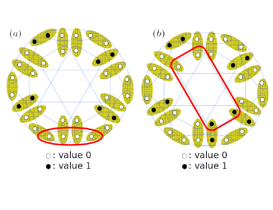
Figure 6.10: Examples of noncontextual assignments of $\{0,1\}$-values to the measurement events in the 18 ray construction where it is not required that every measurement has precisely one outcome that is assigned value 1 and three outcomes that are assigned the value 0. That is, normalization is not respected in these assignments. Example (a) depicts an assignment wherein there is a measurement all of whose outcomes receive probability 0, hence a subnormalized assignment (the probabilities add up to less than 1 for the highlighted measurement). Example (b) depicts one wherein there is a measurement two of whose outcomes recieve probability 1, hence a supernormalized assignment (the probabilities add up to more than 1 for the highlighted measurement).

It is useful to use a notation that specfies whether a given expectation value of some variable $X$ is relative to a preparation procedure $P$, in which case it is denoted $\langle X\rangle_{P}$, or relative to an ontic state $\lambda$, in which case it is denoted $\langle X\rangle_{\lambda}$. We denote by $\alpha^{\prime}(P)$ the quantity defined in (6.52) if the expectation values contained therein are relative to preparation $P$, and we denote by $\alpha^{\prime}(\lambda)$ the case where the expectation values are relative to ontic state $\lambda$. Under the assumption of an ontological model, each expectation value relative to a preparation $P$ can be expressed as a function of the expectation value relative to an ontic state $\lambda$, via

$$\langle X\rangle_{P}=\sum_{\lambda}\langle X\rangle_{\lambda}\;\mu(\lambda|P),$$ (6.54)

where $\mu(\lambda|P)$ is the distribution over ontic states associated with preparation $P$. We can infer from Eq. (6.54) that

$$\alpha^{\prime}(P)=\sum_{\lambda}\alpha^{\prime}(\lambda)\mu(\lambda|P).$$ (6.55)

With these notational conventions, we can summarize the argument of Ref. [70] as follows. In any noncontextual ontological model, every ontic state $\lambda$ satisfies

$$\alpha^{\prime}(\lambda)\leq 8.$$ (6.56)

But this in turn implies, through Eq. (6.55), that for all preparations $P$,

$$\alpha^{\prime}(P)\leq 8,$$ (6.57)

which is an inequality constraining operational quantities. Cabello [70] then goes on to show that this inequality is violated for any quantum state, hence violating this inequality proves “state-independent contextuality”. We will argue that although the violation of this inequality is indeed state-independent, such a violation is not due to contextuality. Instead, this state-independent violation is on account of a fundamental inconsistency in the sort of ontological model that is implicitly assumed in Cabello’s discussion. We will show that the violation of this inequality is necessary for any ontological model – noncontextual or otherwise – to even make sense and that this violation and its state-independence is therefore not a signature of contextuality.

Let us now describe the problem with the inequality (6.57), or equivalently inequality (6.48), and thus with the claim of Ref. [70]. First, we highlight the physical interpretation of the variables $v_{\kappa}$. If $v_{\kappa}$ is assigned value 1 by the ontic state $\lambda$, then this means that if the system is in the ontic state $\lambda$, and a measurement that includes $\kappa$ as an outcome is implemented on it, then the outcome $\kappa$ is certain to occur, while if $v_{\kappa}$ is assigned value 0 by $\lambda$, then the outcome $\kappa$ is certain not to occur. But each of the $2^{18}$ different assignments to $(v_{1},\dots,v_{18})$ is such that for at least one measurement either none of the outcomes occur, as in the example of Fig. 6.10(a), or more than one outcome occurs, as in the example of Fig. 6.10(b). (This is precisely what is implied by the fact that the 18 measurement events are Kochen-Specker KS-uncolourable.) Such assignments involve a logical contradiction given that the four outcomes of each measurement are mutually excusive and jointly exhaustive possibilities.

It follows that the sort of model that a violation of inequality (6.57) rules out can already be ruled out by logic alone; no experiment is required. To put it another way, discovering that quantum theory and nature violate inequality (6.57) only allows one to conclude that neither quantum theory nor nature involve a logical contradiction, which one presumably already knew prior to noting the violation.

We have already argued that the notion of KS-noncontextuality, insofar as it assumes outcome-determinism, is not suitable for devising experimentally robust inequalities given that every real measurement involves some noise. The problem with inequality (6.57) can also be traced back to the use of the assumption of KS-noncontextuality. Suppose we ask the following question: given the existence of nine four-outcome measurements satisfying the operational equivalences of Fig. 6.2(a), how are the operational probabilities that are assigned to these measurement events constrained if we presume that KS-noncontextual assignments underlie the operational statistics? On the face of it, the question seems well-posed. On further reflection, however, one sees that it is not. There are simply no KS-noncontextual assignments to these measurement events, so it is simply impossible to imagine that such assignments could underlie the operational statistics. There is nothing to be tested experimentally, as the hypothesis under consideration is seen to be false as a matter of logic.

Here is another way to see that the inequality (6.57) does not provide a test of noncontextuality. Consider the expectation value $\langle v_{\kappa_{1}}\oplus v_{\kappa_{2}}\oplus v_{\kappa_{3}}\oplus v_{\kappa_{4}}\rangle_{P}$ for a preparation $P$, where $\kappa_{1}$, $\kappa_{2}$, $\kappa_{3}$ and $\kappa_{4}$ correspond to the four outcomes of some measurement. Regardless of which of the four outcomes of the measurement occurs in a given run where preparation $P$ is implemented—i.e. regardless of whether $(v_{\kappa_{1}},v_{\kappa_{2}},v_{\kappa_{3}},v_{\kappa_{4}})$ comes out as (1,0,0,0) or (0,1,0,0) or (0,0,1,0) or (0,0,0,1) in that run—the variable $v_{\kappa_{1}}\oplus v_{\kappa_{2}}\oplus v_{\kappa_{3}}\oplus v_{\kappa_{4}}$ has the value 1. We can think of it this way: the variable $v_{\kappa_{1}}\oplus v_{\kappa_{2}}\oplus v_{\kappa_{3}}\oplus v_{\kappa_{4}}$ is a trivial variable because it is a constant function of the measurement outcome. (This is analogous to how, in quantum theory, for a four-outcome measurement associated with four projectors, although each projector is a nontrivial observable, their sum is the identity operator, which has expectation value 1 for all quantum states, and therefore corresponds to a trivial observable.) It follows that regardless of what distribution over the four outcomes is assigned by $P$, the expectation value $\langle v_{\kappa_{1}}\oplus v_{\kappa_{2}}\oplus v_{\kappa_{3}}\oplus v_{\kappa_{4}}\rangle_{P}$ will be 1. Given that each of the nine terms in $\alpha^{\prime}(P)$ is of this form, it follows that $\alpha^{\prime}(P)=9$.

So, for any operational theory that admits of nine four-outcome measurements with the operational equivalence relations depicted in Fig. 6.2(a), we will find that $\alpha^{\prime}(P)=9$ for all $P$. Therefore, we can conclude that the inequality $\alpha^{\prime}(P)\leq 8$ is violated for all $P$. One can reach this conclusion without ever considering the question of whether the operational predictions can be explained by some underlying noncontextual model.

Another consequence of the triviality of the variables of the form $v_{\kappa_{1}}\oplus v_{\kappa_{2}}\oplus v_{\kappa_{3}}\oplus v_{\kappa_{4}}$ is that the inequality (6.57) can be violated regardless of how noisy the measurements are. Suppose, for instance, that quantum theory describes our experiment, but that the nine four-outcome measurements are not the projective measurements described in Fig. 6.1, but rather noisy versions thereof. For instance, one can imagine that each measurement is associated with a positive operator-valued measure that is the image under a depolarizing map of the projector valued measure associated with the ideal measurement. The amount of depolarization can be taken arbitrarily large and, as long as it is the same amount of depolarization for each of the measurements, the nine noisy measurements that result will still satisfy precisely the same operational equivalences as the original nine, namely, those depicted in Fig. 6.2(a). For such noisy measurements, we can still identify variables $v_{\kappa}$ associated to the eighteen equivalence classes of measurement events, and we still find that regardless of which of the four outcomes of the measurement occurs, the variable $v_{\kappa_{1}}\oplus v_{\kappa_{2}}\oplus v_{\kappa_{3}}\oplus v_{\kappa_{4}}$ has the value 1, so that regardless of what distribution over the four outcomes is assigned by $P$, the expectation value $\langle v_{\kappa_{1}}\oplus v_{\kappa_{2}}\oplus v_{\kappa_{3}}\oplus v_{\kappa_{4}}\rangle_{P}$ will be 1 and therefore $\alpha^{\prime}(P)=9$, which is a violation of the inequality (6.57).

According to the generalized notion of noncontextuality proposed in Ref. [6], if one adds enough noise to the preparations and measurements in an experiment, it always becomes possible to represent the experimental statistics by a noncontextual model. One way to prove this is to note that: (i) if all of the preparations and the measurements in an experiment admit of positive Wigner representations, then, as demonstrated in Ref. [75], the Wigner representation defines a noncontextual model, and (ii) if one adds enough noise to the preparations and measurements, it is possible to ensure that they admit of positive Wigner representations.

This analysis of the effect of noise accords with intuition: noncontextuality is meant to represent a notion of classicality, so that a failure of noncontextuality is only expected to occur in a quantum experiment if one’s experimental operations have a high degree of coherence. It follows that there should always exist a threshold of noise above which an experiment cannot be used to demonstrate the failure of noncontextuality. One can turn this observation into a minimal criterion that should be satisfied by any noncontextuality inequality, that there should exist a threshold of experimental noise above which it cannot be violated.

As we have just noted, the inequality proposed in Ref. [70] fails this minimal criterion. By contrast, the noncontextuality inequality proposed in this chapter identifies such a threshold for the 18 ray construction: the noise must be kept low enough that the average of the measurement predictabilities is above $5/6$. We have even provided an analysis of such noise thresholds for quantum theory in the section on noise robustness of our noncontextuality inequality.

6.6.2 Alternative interpretation

The inequality proposed in Ref. [70] can be given a different interpretation to the one we have just provided. This interpretation is more charitable in some ways, but it still does not vindicate the proposed inequality as delimiting the boundary of noncontextual models.

The idea is to imagine that for each of the nine measurements, there are in fact five rather than four outcomes that are mutually exclusive and jointly exhaustive. Thus, in this interpretation, it is assumed that the hypergraph describing compatibility relations and operational equivalences is not the one of Fig. 6.2(a), but rather a modification wherein there are nine additional nodes—one additional node appended to each of the nine measurements—as depicted in Fig. 6.11(a).

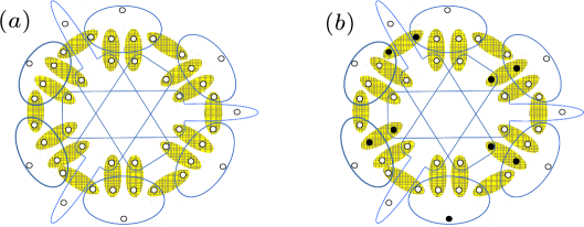
Figure 6.11: (a) The hypergraph wherein each measurement is assigned an additional fifth outcome. (b) A normalized noncontextual deterministic assignment to the hypergraph of (a) that recovers the subnormalized noncontextual deterministic assignment of Fig. 6.10(a) on the appropriate subgraph.

If $\{\kappa_{1},\kappa_{2},\kappa_{3},\kappa_{4}\}$ are the original four outcomes of a given measurement, then the variable $v_{\kappa_{1}}\oplus v_{\kappa_{2}}\oplus v_{\kappa_{3}}\oplus v_{\kappa_{4}}$ is no longer a constant function of the measurement outcome because its value varies depending on whether or not the fifth outcome occurs. If $\kappa_{5}$ denotes the fifth outcome of the measurement, then the trivial variable is $v_{\kappa_{1}}\oplus v_{\kappa_{2}}\oplus v_{\kappa_{3}}\oplus v_{\kappa_{4}}\oplus v_{\kappa_{5}}$, taking the value 1 regardless of the outcome.

In this case, the assignments of the type depicted in Fig. 6.10(a)—the noncontextual deterministic assignments that are subnormalized—can be embedded into noncontextual deterministic normalized assignments on the larger hypergraph, as depicted in Fig. 6.11(b). (The possibility of such an embedding for the subnormalized noncontextual deterministic assignments considered in Cabello, Severini and Winter [25] was noted in Acin, Fritz, Leverrier, Sainz [26].)

Of course, such a move does not provide any way of understanding the deterministic noncontextual assignments of the type depicted in Fig. 6.10(b), because the latter violate normalization by having the probabilities of the different outcomes of the measurement summing to greater than 1—they are supernormalized.

So, while the supernormalized noncontextual deterministic assignments can be ruled out by logic alone, the subnormalized noncontextual deterministic assignments may be entertained without logical inconsistency if they are considered as reductions to a subgraph of a normalized noncontextual deterministic assignment on a larger hypergraph.

Because the justification given in Ref. [70] for the inequality derived there asks one to consider all of the noncontextual deterministic assignments, including the supernormalized ones, the interpretation of this inequality as a constraint on subnormalized assignments is in tension with the manner in which the inequality is justified. This interpretation is a better fit with Cabello’s later work, such as Ref. [25], wherein the restriction to subnormalized assignments is explicit. In any case, if the inequality holds for all noncontextual deterministic assignments, regardless of normalization, then it holds for the special case of the subnormalized assignments, so the inequality can still be derived within this interpretation.

The fundamental problem with this subnormalization interpretation is the following:

While Cabello insists that the quantum model of the experiment involves complete sets of orthonormal rays, thereby implicitly assuming that the operational statistics has no nondetection events, he then allows the response functions corresponding to each basis to be subnormalized in the ontological model, allowing nondetection events when none are seen operationally. This inconsistency – no nondetections in the operational theory, but nondetections in the ontological model – is the reason Cabello’s inequality and its violation don’t signify a failure of KS-noncontextuality. Normalization (no nondetection) in the operational theory is equivalent to normalization (no nondetection) in the ontological model: if the ontological model fails to take this into account, it is a priori ruled out, without even considering the question of its KS-noncontextuality. To see this, note that $p(X|M,P)=\sum_{\lambda}\xi(X|M,\lambda)\mu(\lambda|P)$, and $\sum_{X}p(X|M,P)=1$ if and only if $\sum_{X}\xi(X|M,\lambda)=1$ for all $\lambda$ such that $\mu(\lambda|P)>0$.

Cabello goes on to claim a state-independent violation of his inequality by all quantum states: this is trivially true because of the completeness of the bases chosen and because the scenario is restricted to a 4-dimensional Hilbert space. Any probability assignment induced by the Born rule will then obviously violate Cabello’s inequality: this says nothing about KS-noncontextuality. As we have noted, in order for the subnormalized response functions to make sense, one has to allow the possibility that the operational theory admits nondetection events by, say, considering a 5-dimensional Hilbert space, where the fifth outcome is a nondetection event in each measurement (see Fig. 6.11). In this situation Cabello’s inequality no longer admits a “state-independent” violation: any quantum state that is orthogonal to the 4-dimensional subspace in which the 18 rays live will never violate the inequality, it will just give $\alpha^{\prime}(P)=0$. This means that in a 5-dimensional Hilbert space where subnormalization makes sense, violation of Cabello’s inequality is not “state-independent”, although the violation can be considered a signature of KS-contextuality for the extended hypergraph of Fig. 6.11(a).

It is instructive to compare Cabello’s inequality [70] with the KCBS inequality [35] to understand why the former is not a test of KS-noncontextuality for the 18 ray construction in 4 dimensions (Fig. 6.1(a)) while the latter is a legitimate test of KS-noncontextuality in 3 dimensions. If one thinks of the five projectors in the Klyachko et al. 5-cycle [35], it is the case that adjacent pairs do not add up to identity. Hence it is possible to have a nonzero nondetection probability operationally (corresponding to the projector orthogonal to the subspace defined by an adjacent pair of projectors), and it then makes sense to allow subnormalization in the ontological model and write down the Kochen-Specker type inequality for this case in terms of the independence number [25].

6.7 Experimental testability

Notwithstanding our operationalization of the Kochen-Specker theorem which lets us deal with the problem of noisy measurements, there is still a fundamental difficulty in experimentally testing operational noncontextuality inequalities: namely, the problem of inexact operational equivalences. That is, in general, it will be the case that two experimental procedures (preparations or measurements) that are intended to be operationally equivalent turn out to be only approximately (or inexactly) so. Strictly speaking, we then have no justification for applying the assumption of noncontextuality in the absence of exact operational equivalence. Recall that noncontextuality is an inference from exact operational equivalence in the operational theory to exact ontological equivalence in the ontological model. The equivalence in the ontological model is meant to be a natural explanation of why we see the operational equivalence we see in an experiment. But if such operational equivalences are not seen in the first place, then we have no reason to believe in any ontological equivalence.

A second difficulty – the problem of universal quantifiers – with the experimental testability of operational noncontextuality inequalities is that the number of measurements (preparations) it might take to verify the operational equivalence of a pair of preparation (measurement) procedures can be potentially infinite: this is because we judge operational equivalence of two preparation (measurement) procedures relative to all measurements (preparations) in the operational theory. Unless the operational theory admits of a finite set of tomographically complete preparations and measurements, experimentally verifying the operational equivalence of two procedures would be practically impossible.

In this section we will show how the first difficulty – the problem of inexact operational equivalences – is solved by a convexity argument and the second difficulty – the problem of universal quantifiers – is tackled by assuming the tomographical completeness of a finite number of preparations and measurements. The experiment reported in Ref. [63] looks for violation of a simple operational noncontextuality inequality, not directly related to the traditional Kochen-Specker theorem, that we will derive here. The solution to the problem of inexact operational equivalences that will be discussed here is largely due to Matt Pusey who first came up with the idea reported in Ref. [63]. The methods that resolve these difficulties can be adapted to the test of any operational noncontextuality inequality. In particular, these methods also apply to operational noncontextuality inequalities directly inspired by the Kochen-Specker theorem, such as the one we have already derived in this chapter.

6.7.1 Fair coin flip (FCF) inequality

We will now derive a simple noncontextuality inequality that we call the fair coin flip (FCF) inequality.

The setup

Consider a measurement procedure $M_{*}$ (with outcomes $X\in\{0,1\}$) that is operationally indistinguishable from a fair coin flip, that is,

$$p(X=0|M_{*},P)=p(X=1|M_{*},P)=\frac{1}{2},\forall P\in\mathcal{P}.$$ (6.58)

By the assumption of measurement noncontextuality – namely, if it’s operationally indistinguishable from a fair coin flip then it’s also ontologically indistinguishable from a fair coin flip – we have for the response function

$$\xi(X=0|M_{*},\lambda)=\xi(X=1|M_{*},\lambda)=\frac{1}{2},\forall\lambda\in\Lambda.$$ (6.59)

Consider also three preparation procedures $P_{1},P_{2},P_{3}\in\mathcal{P}$ which are operationally indistinguishable, that is,

$$\forall M\in\mathcal{M}:p(X|M,P_{1})=p(X|M,P_{2})=p(X|M,P_{3}),\text{ where }X\in\{0,1\}.$$ (6.60)

By the assumption of preparation noncontextuality – namely, if the preparation procedures are operationally indistinguishable then they are also ontologically indistinguishable – we have for the associated distributions

$$\forall\lambda\in\Lambda:\mu(\lambda|P_{1})=\mu(\lambda|P_{2})=\mu(\lambda|P_{3}).$$ (6.61)

Suppose that $M_{*}$ can be realized as the uniform mixture of three binary-outcome measurements $M_{1},M_{2},M_{3}\in\mathcal{M}$: that is uniformly randomly pick $t\in\{1,2,3\}$, implement $M_{t}$, and report the outcome of $M_{t}$ as the outcome of $M_{*}$ (coarse graining over $t$).

Suppose also that each preparation procedure $P_{t}\in\mathcal{P}$ can be realized as the uniformly random mixture of two other preparation procedures $P_{t,0},P_{t,1}\in\mathcal{P}$.

Consider an experiment involving a measurement of $M_{t}$ on $P_{t,b}$ (with $b\in\{0,1\}$). We are interested in the average degree of correlation between the outcome $X$ of $M_{t}$ and preparation variable $b$ in $P_{t,b}$:

$$A^{\prime}\equiv\frac{1}{6}\sum_{t\in\{1,2,3\}}\sum_{b\in\{0,1\}}p(X=b|M_{t},P_{t,b}).$$ (6.62)

We will now show that the assumption of noncontextuality places a nontrivial bound on $A^{\prime}$, namely, $A^{\prime}\leq\frac{5}{6}$.

The FCF inequality

Let us first see why we can’t have $A^{\prime}=1$ in a noncontextual ontological model. In order to have $A^{\prime}=1$, we require perfect correlation between $X$ and $b$ for each $M_{t}$ and $P_{t,b}$, i.e. each of the $6$ terms $p(X=b|M_{t},P_{t,b})=1$. This means that any ontic state in the support of $P_{t,b}$ assigns deterministic outcome to $M_{t}$, for otherwise one cannot have $p(X=b|M_{t},P_{t,b})=1$. We therefore have $p(X=0|M_{t},P_{t,0})=p(X=1|M_{t},P_{t,1})=1$. Since $P_{t}$ is an equal mixture of $P_{t,0}$ and $P_{t,1}$, it follows that all the ontic states in the support of $P_{t}$ yield deterministic outcomes for $M_{t}$. The operational equivalence of the three preparation procedures $P_{t}$ then implies that all the ontic states relevant to the experiment (ontic support of any $P_{t}$) assign deterministic outcomes to the three measurements $M_{t}$. In turn, the operational equivalence between $M_{*}$ and a fair coin flip followed by the assumption of measurement noncontextuality applied to this equivalence requires that

$$\forall\lambda\in\Lambda:\frac{1}{3}\xi(X=0|M_{1},\lambda)+\frac{1}{3}\xi(X=0|M_{2},\lambda)+\frac{1}{3}\xi(X=0|M_{3},\lambda)=\frac{1}{2}.$$ (6.63)

Since $M_{t}$ have deterministic response functions, this equation clearly cannot be satisfied, hence we arrive at a contradiction between $A^{\prime}=1$ and the assumption of noncontextuality. To satisfy the condition from measurement noncontextuality at least one of the three response functions has to be indeterministic and that would reduce the degree of correlation to $A^{\prime}<1$. A noncontextual ontological model of such an experiment therefore necessarily requires $A^{\prime}<1$.

A formal proof of the noncontextuality inequality, $A^{\prime}\leq\frac{5}{6}$, follows:

Proof.

In the ontological models framework,

$$A^{\prime}=\sum_{\lambda\in\Lambda}\frac{1}{6}\sum_{t\in\{1,2,3\}}\sum_{b\in\{0,1\}}\xi(X=b|M_{t},\lambda)\mu(\lambda|P_{t,b}).$$ (6.64)

There is an upper bound on each response function that is independent of the value of $b$, namely,

$$\xi(X=b|M_{t},\lambda)\leq\eta(M_{t},\lambda),$$ (6.65)

where

$$\eta(M_{t},\lambda)\equiv\max_{b^{\prime}\in\{0,1\}}\xi(X=b^{\prime}|M_{t},\lambda).$$ (6.66)

We therefore have

$$A^{\prime}\leq\frac{1}{3}\sum_{t\in\{1,2,3\}}\sum_{\lambda\in\Lambda}\eta(M_{t},\lambda)\left(\frac{1}{2}\sum_{b\in\{0,1\}}\mu(\lambda|P_{t,b})\right),$$ (6.67)

Recalling that $P_{t}$ is an equal mixture of $P_{t,0}$ and $P_{t,1}$, so that

$$\mu(\lambda|P_{t})=\frac{1}{2}\mu(\lambda|P_{t,0})+\frac{1}{2}\mu(\lambda|P_{t,1}),$$ (6.68)

we can rewrite the bound as simply

$$A^{\prime}\leq\frac{1}{3}\sum_{t\in\{1,2,3\}}\sum_{\lambda\in\Lambda}\eta(M_{t},\lambda)\mu(\lambda|P_{t}).$$ (6.69)

But recalling Eq. (6.61) (preparation noncontextuality),

$$\forall\lambda\in\Lambda:\mu(\lambda|P_{1})=\mu(\lambda|P_{2})=\mu(\lambda|P_{3}),$$ (6.70)

we see that the distribution $\mu(\lambda|P_{t})$ is independent of $t$, so we denote it by $\nu(\lambda)$ and rewrite the bound as

$$A^{\prime}\leq\sum_{\lambda\in\Lambda}\left(\frac{1}{3}\sum_{t\in\{1,2,3\}}\eta(M_{t},\lambda)\right)\nu(\lambda).$$ (6.71)

This last step is the first use of noncontextuality in the proof because Eq. (6.70) is derived from preparation noncontextuality and the operational equivalence of Eq. (6.60). It then follows that

$$A^{\prime}\leq\max_{\lambda\in\Lambda}\left(\frac{1}{3}\sum_{t\in\{1,2,3\}}\eta(M_{t},\lambda)\right).$$ (6.72)

Therefore, if we can provide a nontrivial upper bound on $\frac{1}{3}\sum_{t}\eta(M_{t},\lambda)$ for an arbitrary ontic state $\lambda$, we obtain a nontrivial upper bound on $A^{\prime}$. We infer constraints on the possibilities for the triple $(\eta(M_{1},\lambda),\eta(M_{2},\lambda),\eta(M_{3},\lambda))$ from constraints on the possibilities for the triple $(\xi(X\text{=}0|M_{1},\lambda),\xi(X\text{=}0|M_{2},\lambda),\xi(X\text{=}0|M_{3},\lambda))$.

The latter triple is constrained by measurement noncontextuality as

$$\frac{1}{3}\sum_{t\in\{1,2,3\}}\xi(X\text{=}0|M_{t},\lambda)=\frac{1}{2}.$$ (6.73)

This is the second use of noncontextuality in our proof, because Eq. (6.73) is derived from the operational equivalence of Eq. (6.58) and the assumption of measurement noncontextuality (Eqs. (6.59,6.63)).

The fact that the range of each response function is $[0,1]$ implies that the vector

$$(\xi(X\text{=}0|M_{1},\lambda),\allowbreak\xi(X\text{=}0|M_{2},\lambda),\xi(X\text{=}0|M_{3},\lambda))$$

is constrained to the unit cube. The linear constraint of Eq. (6.73) implies that these vectors are confined to a two-dimensional plane. The intersection of the plane and the cube defines the polygon depicted in Fig. 6.12.

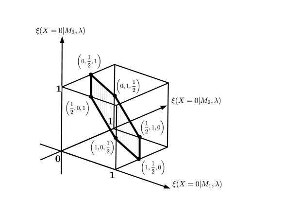
Figure 6.12: The possible values of $(\xi(X\text{=}0|M_{1},\lambda),\xi(X\text{=}0|M_{2},\lambda),\xi(X\text{=}0|M_{3},\lambda))$.

The six vertices of this polygon have coordinates that are a permutation of $(1,\frac{1}{2},0)$. For every $\lambda$, the vector

$$(\xi(X\text{=}0|M_{1},\lambda),\xi(X\text{=}0|M_{2},\lambda),\xi(X\text{=}0|M_{3},\lambda))$$

corresponds to a point in the convex hull of these extreme points and given that $\frac{1}{3}\sum_{t}\eta(M_{t},\lambda)$ is a convex function of this vector, it suffices to find a bound on the value of this function at the extreme points. If $\lambda$ corresponds to the extreme point

$$(\xi(X\text{=}0|M_{1},\lambda),\xi(X\text{=}0|M_{2},\lambda),\xi(X\text{=}0|M_{3},\lambda))=(1,\frac{1}{2},0),$$

then we have $(\eta(M_{1},\lambda),\eta(M_{2},\lambda),\eta(M_{3},\lambda))=(1,\frac{1}{2},1)$, and the other extreme points are simply permutations thereof. It follows that

$$\frac{1}{3}\sum_{t}\eta(M_{t},\lambda)\leq\frac{5}{6}.$$ (6.74)

Substituting this bound into Eq. (6.72), we have our result. ∎

Tightness of bound: two ontological models

We now provide an explicit example of a noncontextual ontological model that saturates our noncontextuality inequality, thus proving that the noncontextuality inequality is tight, i.e., the upper bound of the inequality cannot be reduced any further for a noncontextual model.

We also provide an example of an ontological model that is preparation noncontextual but fails to be measurement noncontextual (i.e. it is measurement contextual) and that exceeds the bound of our noncontextuality inequality. This makes it clear that preparation noncontextuality alone does not suffice to justify the precise bound in our inequality, the assumption of measurement noncontextuality is a necessary ingredient as well.

Note that there is no point inquiring about the bound for models that are measurement noncontextual but preparation contextual because, as shown in Ref. [6], quantum theory admits of models of this type—the ontological model wherein the pure quantum states are the ontic states (the $\psi$-complete ontological model in the terminology of Ref. [1]) is of this sort.

For the two ontological models we present, we begin by specifying the ontic state space $\Lambda$. These are depicted in Figs. 6.13 and 6.14 as pie charts with each slice corresponding to a different element of $\Lambda$. We specify the six preparations $P_{t,b}$ by the distributions over $\Lambda$ that they correspond to, denoted $\mu(\lambda|P_{t,b})$ (middle left of Figs. 6.13 and 6.14). We specify the three measurements $M_{t}$ by the response functions for the $X=0$ outcome, denoted $\xi(0|M_{t},\lambda)$ (top right of Figs. 6.13 and 6.14). Finally, we compute the operational probabilities for the various preparation-measurement pairs, using $p(X|M,P)=\sum_{\lambda\in\Lambda}\xi(X|M,\lambda)\mu(\lambda|P)$, and display the results in the $6\times 4$ upper-left-hand corner of Tables 6.6 and 6.7.

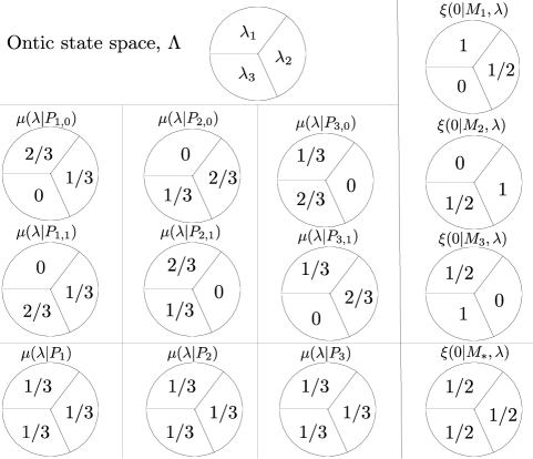
Figure 6.13: A noncontextual ontological model that saturates the noncontextal bound of our inequality, exhibiting that the bound is tight.

	$[0|M_{1}]$	$[0|M_{2}]$	$[0|M_{3}]$	$[0|M_{*}]$
$P_{1,0}$	$5/6$	$1/3$	$1/3$	$1/2$
$P_{1,1}$	$1/6$	$2/3$	$2/3$	$1/2$
$P_{2,0}$	$1/3$	$5/6$	$1/3$	$1/2$
$P_{2,1}$	$2/3$	$1/6$	$2/3$	$1/2$
$P_{3,0}$	$1/3$	$1/3$	$5/6$	$1/2$
$P_{3,1}$	$2/3$	$2/3$	$1/6$	$1/2$
$P_{1}$	$1/2$	$1/2$	$1/2$	$1/2$
$P_{2}$	$1/2$	$1/2$	$1/2$	$1/2$
$P_{3}$	$1/2$	$1/2$	$1/2$	$1/2$

Table 6.6: Operational statistics from the noncontextual ontological model of Fig. 6.13, achieving $A^{\prime}=5/6$. The shaded cells correspond to the ones relevant for calculating $A^{\prime}$.

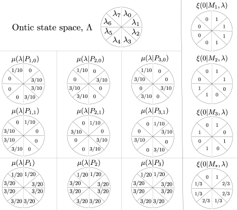
Figure 6.14: An ontological model that is preparation noncontextual but measurement contextual and that violates our inequality.

	$[0|M_{1}]$	$[0|M_{2}]$	$[0|M_{3}]$	$[0|M_{*}]$
$P_{1,0}$	$9/10$	$3/10$	$3/10$	$1/2$
$P_{1,1}$	$1/10$	$7/10$	$7/10$	$1/2$
$P_{2,0}$	$3/10$	$9/10$	$3/10$	$1/2$
$P_{2,1}$	$7/10$	$1/10$	$7/10$	$1/2$
$P_{3,0}$	$3/10$	$3/10$	$9/10$	$1/2$
$P_{3,1}$	$7/10$	$7/10$	$1/10$	$1/2$
$P_{1}$	$1/2$	$1/2$	$1/2$	$1/2$
$P_{2}$	$1/2$	$1/2$	$1/2$	$1/2$
$P_{3}$	$1/2$	$1/2$	$1/2$	$1/2$

Table 6.7: Operational statistics from the preparation noncontextual and measurement contextual ontological model of Fig. 6.14, achieving $A^{\prime}=9/10$. The shaded cells correspond to the ones relevant for calculating $A^{\prime}$.

In the remainder of each table, we display the operational probabilities for the effective preparations, $P_{t}$, which are computed from the operational probabilities for the $P_{t,b}$ and the fact that $P_{t}$ is the uniform mixture of $P_{t,0}$ and $P_{t,1}$. We also display the operational probabilities for the effective measurement $M_{*}$, which is computed from the operational probabilities for the $M_{t}$ and the fact that $M_{*}$ is a uniform mixture of $M_{1}$, $M_{2}$ and $M_{3}$.

From the tables, we can verify that our two ontological models imply the operational equivalences that we use in the derivation of our noncontextuality inequality. Specifically, the three preparations $P_{1}$, $P_{2}$ and $P_{3}$ yield exactly the same statistics for all of the measurements, and the measurement $M_{*}$ is indistinguishable from a fair coin flip for all the preparations.

Figs. 6.13 and 6.14 also depict $\mu(\lambda|P_{t})$ for $t\in\{1,2,3\}$ for each model (bottom left). These are determined from the $\mu(\lambda|P_{t,b})$ via Eq. (6.68). Similarly, the response function $\xi(0|M_{*},\lambda)$, which is determined from $\xi(X=b|M_{*},\lambda)=\frac{1}{3}\sum_{t\in\{1,2,3\}}\xi(X=b|M_{t},\lambda)$, is displayed in each case (bottom right).

Given the operational equivalence of $P_{1}$, $P_{2}$ and $P_{3}$, an ontological model is preparation noncontextual if and only if $\mu(\lambda|P_{1})=\mu(\lambda|P_{2})=\mu(\lambda|P_{3})$ for all $\lambda\in\Lambda$. We see, therefore, that both models are preparation noncontextual. Similarly given the operational equivalence of $M_{*}$ and a fair coin flip, an ontological model is measurement noncontextual if and only if $\xi(0|M_{*},\lambda)=\frac{1}{2}$ for all $\lambda\in\Lambda$. We see, therefore, that only the first model is measurement noncontextual. Note that in the second model, $M_{*}$ manages to be operationally equivalent to a fair coin flip, despite the fact that when one conditions on a given ontic state $\lambda$, it does not have a uniformly random response. This is possible only because the set of distributions is restricted in scope, and the overlaps of these distributions with the response functions always generates the uniformly random outcome. This highlights how an ontological model can do justice to the operational probabilities while failing to be noncontextual.

Finally, using the operational probabilities in the tables, one can compute the value of $A^{\prime}$ for each model. It is determined entirely by the operational probabilities in the shaded cells. One thereby confirms that $A^{\prime}=\frac{5}{6}$ in the first model, while $A^{\prime}=\frac{9}{10}$ in the second model.

Quantum violation of the noncontextuality inequality

Quantum theory predicts that there is a set of preparations and measurements on a qubit having the supposed properties and achieving $A^{\prime}=1$, maximally violating the noncontextuality inequality. Take the $M_{t}$ to be represented by the observables $\vec{\sigma}\cdot\hat{n}_{t}$ where $\vec{\sigma}$ is the vector of Pauli operators and the unit vectors $\{\hat{n}_{1},\hat{n}_{2},\hat{n}_{3}\}$ are separated by 120^∘ in the $\hat{x}-\hat{z}$ plane of the Bloch sphere of qubit states. The $P_{t,b}$ are the eigenstates of these observables, where we associate the positive eigenstate $|\text{+}\hat{n}_{t}\rangle\langle+\hat{n}_{t}|$ with $b=0$. To see that the statistical equivalence of Eq. (6.58) is satisfied, it suffices to note that

$$\frac{1}{3}|\text{+}\hat{n}_{1}\rangle\langle\text{+}\hat{n}_{1}|+\frac{1}{3}|\text{+}\hat{n}_{2}\rangle\langle\text{+}\hat{n}_{2}|+\frac{1}{3}|\text{+}\hat{n}_{3}\rangle\langle\text{+}\hat{n}_{3}|=\frac{1}{2}\mathbb{I},$$ (6.75)

and to recall that for any density operator $\rho$, ${\rm tr}(\rho\frac{1}{2}\mathbb{I})=\frac{1}{2}$. To see that the statistical equivalence of Eq. (6.60) is satisfied, it suffices to note that for all pairs $t,t^{\prime}\in\{1,2,3\}$,

$$\frac{1}{2}|\text{+}\hat{n}_{t}\rangle\langle\text{+}\hat{n}_{t}|+\frac{1}{2}|{-}\hat{n}_{t}\rangle\langle{-}\hat{n}_{t}|$$

$$=\frac{1}{2}|\text{+}\hat{n}_{t^{\prime}}\rangle\langle\text{+}\hat{n}_{t^{\prime}}|+\frac{1}{2}|{-}\hat{n}_{t^{\prime}}\rangle\langle{-}\hat{n}_{t^{\prime}}|,$$ (6.76)

which asserts that the average density operator for each value of $t$ is the same, and therefore leads to precisely the same statistics for all measurements. Finally, it is clear that the outcome of the measurement of $\vec{\sigma}\cdot\hat{n}_{t}$ is necessarily perfectly correlated with whether the state was $|\text{+}\hat{n}_{t}\rangle\langle\text{+}\hat{n}_{t}|$ or $|{-}\hat{n}_{t}\rangle\langle{-}\hat{n}_{t}|$, so that $A^{\prime}=1$.

These quantum measurements and preparations are what we seek to implement experimentally, so we refer to them as ideal, and denote them by $M^{\rm i}_{t}$ and $P^{\rm i}_{t,b}$. However, since we want our analysis of the data to be theory-independent, we will have to explicitly verify the relevant operational equivalences instead of taking them for granted as we do in quantum theory.

Note that our noncontextuality inequality can accommodate noise in both the measurements and the preparations, up to the point where the average of $p(X=b|M_{t},P_{t,b})$ drops below $\frac{5}{6}$. It is in this sense that our inequality does not presume the idealization of noiseless measurements.

6.7.2 Tackling the problem of inexact operational equivalences: Secondary procedures

Let us recall the problem of inexact operational equivalence: two experimental procedures are seen to be “close” to operationally equivalent but not quite exactly equivalent and the assumption of noncontextuality then cannot, strictly speaking, be applied in the absence of exact operational equivalence. Our general solution to this problem with experimental tests of noncontextuality, first implemented explicitly for a particular test in the experiment of Ref. [63], is described in the following steps:

1. Raw data matrix: Take the set of experimental procedures (preparations or measurements) that are implemented in the laboratory and for which the raw data is collected. Tabulate the raw data in a matrix $\mathbb{D}^{r}$ with entries $\{f_{ij}\}$, where $f_{ij}$ is the fraction of $[0|M_{i}]$ outcomes that occur when binary-outcome measurement procedure $M_{i}$, with outcome set $\{0,1\}$, is implemented following preparation procedure $P_{j}$:

   $$\mathbb{D}^{r}=\begin{pmatrix}f_{11}&f_{12}&\dots&f_{1n}\\ f_{21}&f_{22}&\dots&f_{2n}\\ \vdots\\ f_{m1}&f_{m2}&\dots&f_{mn}\end{pmatrix},$$ (6.77)

   where we consider an experiment in which $m$ binary-outcome measurements are implemented on each of $n$ preparations. Each row denotes a measurement procedure while each column denotes a preparation procedure in this matrix of raw data. We assume that the primary measurement and preparation procedures implemented in the laboratory to obtain this raw data arise from a generalized probabilistic theory (GPT) in which $m_{t}$ ($\leq m$) of the $m$ measurements implemented are tomographically complete. This assumption is necessary because verifying the operational equivalence between two preparations requires that we implement a tomographically complete set of measurements. We will obtain estimates of the probabilities associated with the primary procedures by fitting the raw data (which is obtained from a large but finite number of runs of the experiment) to this GPT.

   In the experiment of Ref. [63], we have $m=4$ and $n=8$, and we have assumed $m_{t}=3$.

2. Estimating probabilities (fitting raw data to GPT): Assuming that a finite number, $m_{t}$, of independent binary-outcome measurements are tomographically complete, we fit the raw data in $\mathbb{D}^{r}$ to a matrix $\mathbb{D}^{\rm p}$ of estimated probabilities arising from a GPT with $m_{t}$ tomographically complete measurements. As with $\mathbb{D}^{r}$, the rows of $\mathbb{D}^{\rm p}$ denote the primary measurements and the columns of $\mathbb{D}^{\rm p}$ denote the primary preparations. We will describe the fitting procedure later. The entries of $\mathbb{D}^{\rm p}$ are given by $p_{ij}\equiv p(0|M_{i}^{\rm p},P_{j}^{\rm p})$, i.e. $p_{ij}$ are the estimated probabilities – given the raw frequencies in $\mathbb{D}^{r}$ – of outcome $[0|M_{i}^{\rm p}]$ of measurement procedure $M_{i}^{\rm p}$ following preparation procedure $P_{j}^{\rm p}$:

   $$\mathbb{D}^{\rm p}=\begin{pmatrix}p_{11}&p_{12}&\dots&p_{1n}\\ p_{21}&p_{22}&\dots&p_{2n}\\ \vdots\\ p_{m1}&p_{m2}&\dots&p_{mn}\end{pmatrix}.$$ (6.78)

3. Failure of exact operational equivalences: The primary measurement and preparation procedures will typically fail to satisfy – by however small a margin – the operational equivalences required in a particular test of noncontextuality. Can one salvage anything interesting from the primary data despite this failure of exact operational equivalences? Yes: by inferring secondary procedures.

4. Secondary procedures (restoring exact operational equivalences): For the set of primary procedures, consider their convex hull, i.e. the set of all procedures that can be obtained from the primary set by probabilistically mixing the elements of the primary set. Since all these procedures constitute post-processing of the probabilities estimated from the raw data, we can define secondary procedures corresponding to the primary procedures such that for each primary procedure relevant to the noncontextuality inequality we have a secondary procedure that is as close as possible to the primary procedure but which is chosen so that the operational equivalences required for testing noncontextuality are exactly satisfied for the chosen set of secondary procedures. Being able to find such a set of secondary procedures signals a good experiment that can meaningfully test noncontextuality: if such secondary procedures cannot be found, then the data will have to be discarded and the experiment repeated more carefully. This needs to be done only for those procedures (preparations and /or measurements) which are required to satisfy some operational equivalences for the particular test of noncontextuality.

   In the case of preparations, the post-processing involves probabilistic mixtures of the primary preparation procedures (the columns of $\mathbb{D}^{\rm p}$, denoted by ${\bf P}^{\rm p}_{k}$ with $k=1,\dots,n$) to define the secondary preparation procedures (the columns of secondary data matrix $\mathbb{D}^{\rm s}$, denoted by ${\bf P}^{\rm s}_{j}$ with $j=1,\dots,n^{\prime}$, $n^{\prime}\leq n$):

   $${\bf P}^{\rm s}_{j}=\sum_{k=1}^{n}u_{jk}{\bf P}^{\rm p}_{k},\text{ where }u_{jk}\geq 0\quad\forall j,k,\text{ and }\sum_{k}u_{jk}=1\quad\forall j\in\{1,2,\dots,n^{\prime}\}.$$ (6.79)

   To keep the secondary preparation procedures as close as possible to the primary ones, we maximize the function

   $$C_{\rm P}\equiv\frac{1}{n^{\prime}}\sum_{j=1}^{n^{\prime}}u_{jj},$$ (6.80)

   subject to the constraints imposed by the operational equivalences required between the preparation procedures for the particular test of noncontextuality.

   In the case of measurements, extremal post-processings of primary events $[0|M_{l}^{\rm p}]$ also include: 1) relabelling the outcomes of a measurement $M_{l}^{\rm p}$ to define a flipped-outcome measurement $M_{\lnot l}^{\rm p}$ such that $[X|M_{l}^{\rm p}]\simeq[1-X|M_{\lnot l}^{\rm p}]$, $X\in\{0,1\}$, 2) the measurement event that is certain to occur (i.e. obtaining outcome ‘0’ for all preparation procedures), denoted by a row vector 1 with all probabilities $1$, 3) the measurement event that is certain not to occur (i.e. not obtaining outcome ‘0’ for any of the preparation procedures or, equivalently, obtaining outcome ‘1’ for all preparation procedures), denoted by a row vector 0 with all probabilities $0$. The secondary measurement procedures (the rows of secondary data matrix $\mathbb{D}^{\rm s}$, denoted by ${\bf M}^{\rm s}_{i}$ with $i=1,\dots,m^{\prime}$, $m^{\prime}\leq m$) are obtained by probabilistic mixing of all the primary events $[0|M_{l}^{\rm p}]$ (denoted by row vectors ${\bf M}^{\rm p}_{l}$ with $l=1,\dots,m$) with their extremal post-processings $[0|M_{\lnot l}^{\rm p}]$ (denoted by row vectors ${\bf 1}-{\bf M}^{\rm p}_{l}$ with $l=1,\dots,m$), 0, and 1 events:

   $${\bf M}^{\rm s}_{i}=\sum_{l=1}^{m}v_{il}{\bf M}^{\rm p}_{l}+v_{i0}{\bf 0}+v_{i1}{\bf 1}+\sum_{l^{\prime}=1}^{m}v_{i,\lnot l^{\prime}}({\bf 1}-{\bf M}^{\rm p}_{l^{\prime}}),$$ (6.81)

   where $\sum_{l=1}^{m}v_{il}+v_{i0}+v_{i1}+\sum_{l^{\prime}=1}^{m}v_{i,\lnot l^{\prime}}=1$ for all $i$ and all the weights $v_{il},v_{i,\lnot l^{\prime}},v_{i0},v_{i1}$ are nonnegative. Note that the purpose of allowing mixtures of 0, 1, and ${\bf 1}-{\bf M}^{\rm p}_{l}$ besides the original set of ${\bf M}^{\rm p}_{l}$ is to permit greater freedom in the choice of secondary measurement procedures that can satisfy all the required operational equivalences exactly and are also as close as possible to the primary set of measurement procedures. The latter requirement is motivated by the fact that an experimenter intends to implement primary procedures – both preparations and measurements – that maximize the violation of noncontextuality, hence we want to infer secondary procedures as close to the intended ones as possible while at the same time satisfying the prerequisite of exact operational equivalences for a test of noncontextuality.

   To keep the secondary measurement procedures as close as possible to the primary ones, we maximize the function

   $$C_{\rm M}\equiv\frac{1}{m^{\prime}}\sum_{i=1}^{m^{\prime}}v_{ii},$$ (6.82)

   subject to the constraints imposed by the operational equivalences required between the measurement procedures for the particular test of noncontextuality.

   All in all, the entries $s_{ij}\equiv p(0|M^{\rm s}_{i},P^{\rm s}_{j})$ of the $m^{\prime}\times n^{\prime}$ secondary data matrix $\mathbb{D}^{\rm s}$ are given by:

   $$s_{ij}=\sum_{k=1}^{n}u_{jk}\left[\sum_{l=1}^{m}v_{il}p_{lk}+v_{i0}0+v_{i1}1+\sum_{l^{\prime}=1}^{m}v_{i,\lnot l^{\prime}}\left(1-p_{l^{\prime}k}\right)\right]$$ (6.83)

   These entries belonging to $\mathbb{D}^{\rm s}$ are the ones that are finally used in checking whether a particular noncontextuality inequality is violated or not, since they satisfy the required operational equivalences exactly.

   In the experiment of Ref. [63], $m^{\prime}=3$ and $n^{\prime}=6$ and the relevant operational equivalences that need to be exactly satisfied are those of Eqs. (6.58) and (6.60).

Note that in describing this algorithm for handling failure of operational equivalence, we have not restricted ourselves to the FCF inequality, although the only known experiment (so far) where this algorithm has been implemented tests the FCF inequality [63]. This algorithm should work, in principle, for any test of a noncontextuality inequality including the one inspired by the Kochen-Specker theorem derived earlier in this chapter. It is our hope that describing this algorithm in general terms will help carry out robust experimental tests of noncontextuality in the spirit of the experiment of Ref. [63].

Estimating $\mathbb{D}^{\rm p}$: fitting raw data to GPT

To fit the raw data matrix $\mathbb{D}^{r}$ to a matrix $\mathbb{D}^{\rm p}$ arising from a GPT, we first need to characterize the set of $\mathbb{D}^{\rm p}$ that can arise from a GPT with a specified number of tomographically complete effects. The following theorem characterizes such $\mathbb{D}^{\rm p}$:

Theorem 11.

A matrix $\mathbb{D}^{\rm p}$ with rows corresponding to effects

$$\left\{[0|M_{1}],[0|M_{2}],\dots,[0|M_{m}]\right\}$$

can arise from a GPT in which $m_{t}=|\mathcal{M}_{\rm tomo}|<m$ of these effects, say

$$\mathcal{M}_{\rm tomo}\equiv\left\{[0|M_{1}],[0|M_{2}],\dots,[0|M_{m_{t}}]\right\},$$

are tomographically complete if and (with a measure zero set of exceptions) only if

$$\forall c\in\{m_{t}+1,m_{t}+2,\dots,m\}:\sum_{i=1}^{m_{t}}a_{ci}p_{ij}+a_{c}p_{cj}-1=0\quad\forall j\in\{1,2,\dots,n\},$$ (6.84)

for some real constants $\{a_{c1},a_{c2},\dots,a_{cm_{t}},a_{c}\}_{c=m_{t}+1}^{m}$. This set of $m-m_{t}$ (one for each value of $c$) linear constraints characterize the set of $m\times n$ matrices $\mathbb{D}^{\rm p}$ arising from a GPT with $m_{t}$ tomographically complete effects.

Proof.

“only if”: We assume that $\mathbb{D}^{\rm p}$ belongs to a GPT with $m_{t}=|\mathcal{M}_{\rm tomo}|$ tomographically complete measurements. Let $\mathcal{M}_{\rm tomo}=\{M_{1}^{\rm p},M_{2}^{\rm p},\dots,M_{m_{t}}^{\rm p}\}$ be such a set of fiducial measurements tomographically complete for a system, so that the state of the system given a preparation procedure $P$ is specified by the column vector

$${\bf p}_{P}=\begin{pmatrix}1\\ p(0|M_{1}^{\rm p},P)\\ p(0|M_{2}^{\rm p},P)\\ \vdots\\ p(0|M_{m_{t}}^{\rm p},P)\end{pmatrix},$$ (6.85)

where the first entry ensures normalization of the state. As shown in Refs. [67, 68], convexity then requires that the probability of outcome ‘0’ for any measurement $M\in\mathcal{M}$ is given by ${\bf r}_{M}.{\bf p}_{P}$ for some vector ${\bf r}_{M}$. Let $\{{\bf r}_{1},{\bf r}_{2},\dots,{\bf r}_{m}\}$ denote the vectors corresponding to outcome ‘0’ of the measurements $\{M_{1}^{\rm p},M_{2}^{\rm p},\dots,M_{m}^{\rm p}\}$ respectively. The measurement event that always occurs (e.g. the event of obtaining outcome ‘0’ or ‘1’ in any binary-outcome measurement) must be represented by ${\bf r}_{\mathbb{I}}=(1,0,0,\dots,0)\in\mathbb{R}^{m_{t}+1}$ (so that ${\bf r}_{\mathbb{I}}.{\bf p}_{P}=1$ for all $P\in\mathcal{P}$).

Note that in order to have an experiment that allows for operational equivalences to be verified, the number of measurements carried out in the experiment, $m$, must be at least as large as the cardinality of the tomographically complete set of measurements, $m_{t}$, i.e. $m\geq m_{t}$. We will therefore presume that our experimental test of noncontextuality has $m>m_{t}$ in what follows. Since $\{\{{\bf r}_{i}\}_{i=1}^{m},{\bf r}_{\mathbb{I}}\}$ is a set of $m+1$ vectors in $\mathbb{R}^{m_{t}+1}$, any $m_{t}+2$ element subset of them, say $\{{\bf r}_{1},\dots,{\bf r}_{m_{t}},{\bf r}_{\mathbb{I}},{\bf r}_{c}\}$, must necessarily be linearly dependent:

$$\sum_{i=1}^{m_{t}}a^{\prime}_{ci}{\bf r}_{i}+a^{\prime}_{c}{\bf r}_{c}+e^{\prime}_{c}{\bf r}_{\mathbb{I}}=0,$$ (6.86)

with $(a^{\prime}_{c1},a^{\prime}_{c2},\dots,a^{\prime}_{cm_{t}},a^{\prime}_{c},e^{\prime}_{c})\neq(0,0,\dots,0,0,0)$. The set of $\{\{{\bf r}_{i}\}_{i=1}^{m_{t}},{\bf r}_{c},{\bf r}_{\mathbb{I}}\}$ for which $e^{\prime}_{c}=0$ are those where ${\bf r}_{\mathbb{I}}$ is not in the span of $\{\{{\bf r}_{i}\}_{i=1}^{m_{t}},{\bf r}_{c}\}$, which is a set of measure zero. To see this, note that the set of vectors $\{{\bf r}_{\mathbb{I}},{\bf r}_{1},{\bf r}_{2},\dots,{\bf r}_{m_{t}}\}$ forms an orthonormal basis for $\mathbb{R}^{m_{t}+1}$, where ${\bf r}_{i}=(0,\dots,1,\dots,0)$ ($i+1$th entry 1, rest 0) represents the measurement $M_{i}^{\rm p}$ from the fiducial set. Any ${\bf r}_{i}$ should be expressible as a linear combination of $\{\{{\bf r}_{i}\}_{i=1}^{m_{t}},{\bf r}_{\mathbb{I}}\}$. Restricting the set $\{\{{\bf r}_{i}\}_{i=1}^{m_{t}},{\bf r}_{c}\}$ to the subspace orthogonal to ${\bf r}_{\mathbb{I}}$ — so that $e^{\prime}_{c}=0$ and ${\bf r}_{\mathbb{I}}$ is not in the span of $\{\{{\bf r}_{i}\}_{i=1}^{m_{t}},{\bf r}_{c}\}$ — means that the $\{\{{\bf r}_{i}\}_{i=1}^{m_{t}},{\bf r}_{c}\}$ lie in a one dimension lower subspace $\mathbb{R}^{m_{t}}$ of $\mathbb{R}^{m_{t}+1}$, hence they form a measure zero set. Therefore, we can generically ensure $e^{\prime}_{c}\neq 0$ and divide throughout by $-e^{\prime}_{c}$ to obtain

$$\sum_{i=1}^{m_{t}}a_{ci}{\bf r}_{i}+a_{c}{\bf r}_{c}-{\bf r}_{\mathbb{I}}=0,\text{ where }a_{c}=-a^{\prime}_{c}/e^{\prime}_{c},a_{ci}=-a^{\prime}_{ci}/e^{\prime}_{c}\quad\forall i.$$ (6.87)

Let ${\bf p}_{j}$ denote the vector representing preparation $P_{j}^{\rm p}$, then we have $p_{ij}={\bf r}_{i}.{\bf p}_{j}$, where $p_{ij}=p(0|M^{\rm p}_{i},P^{\rm p}_{j})$ is the $(i,j)$th entry of $\mathbb{D}^{\rm p}$. Taking dot product with ${\bf p}_{j}$, we then have

$$\sum_{i=1}^{m_{t}}a_{ci}p_{ij}+a_{c}p_{cj}-1=0$$ (6.88)

for some real constants $\{a_{c1},a_{c2},\dots,a_{cm_{t}},a_{c}\}$, for every $c\in\{m_{t}+1,\dots,m\}$. We now prove the converse.

“if”: Since we require some subset of $\{M_{1}^{\rm p},M_{2}^{\rm p},\dots,M_{m}^{\rm p}\}$ to be a fiducial set in order to be able to verify operational equivalences for a test of noncontextuality (recall that $m>m_{t}$ is a necessary condition for this), we take $\{M_{1}^{\rm p},M_{2}^{\rm p},\dots,M_{m_{t}}^{\rm p}\}$ to be a fiducial set of measurements as before, so that preparation procedure $P_{j}^{\rm p}$ corresponds to the vector

$${\bf p}_{j}=\begin{pmatrix}1\\ p_{1j}\\ p_{2j}\\ \vdots\\ p_{m_{t}j}\end{pmatrix},$$ (6.89)

where $p_{ij}=p(0|M^{\rm p}_{i},P^{\rm p}_{j})$.

Now we can recover $\mathbb{D}^{\rm p}$ if $M_{i}^{\rm p}$ ($i=1,\dots,m_{t}$) is represented by ${\bf r}_{i}=(0,\dots,0,1,0,\dots,0)$ ($(i+1)$th entry 1 and the rest 0), so that $p_{ij}={\bf r}_{i}.{\bf p}_{j}$ for $i\in\{1,\dots,m_{t}\}$ and, since we are given $\sum_{i=1}^{m_{t}}a_{ci}p_{ij}+a_{c}p_{cj}-1=0$ for every $c\in\{m_{t}+1,\dots,m\}$, we must have

$$\sum_{i=1}^{m_{t}}a_{ci}p_{ij}+a_{c}p_{cj}-1=0\Leftrightarrow\left(\sum_{i=1}^{m_{t}}a_{ci}{\bf r}_{i}+a_{c}{\bf r}_{c}-{\bf r}_{\mathbb{I}}\right).{\bf p}_{j}=0.$$ (6.90)

That is

$$a_{c}{\bf r}_{c}.{\bf p}_{j}=-\left(\sum_{i=1}^{m_{t}}a_{ci}{\bf r}_{i}-{\bf r}_{\mathbb{I}}\right).{\bf p}_{j},$$ (6.91)

so that we can take

$${\bf r}_{c}=(1/a_{c},-a_{c1}/a_{c},-a_{c2}/a_{c},\dots,-a_{cm_{t}}/a_{c})$$ (6.92)

for every $c\in\{m_{t}+1,\dots,m\}$ and thus reconstruct the $m\times n$ matrix $\mathbb{D}^{\rm p}$. This proves the converse. We therefore have a characterization of $\mathbb{D}^{\rm p}$. ∎

Geometrically, this theorem means that the $n$ columns of $\mathbb{D}^{\rm p}$ – each represented by a vector ${\bf p}_{j}\in\mathbb{R}^{m_{t}+1}$ – lie in the common intersection of $m_{t}$-dimensional hyperplanes ($m-m_{t}$ of them) defined by the constants

$$\{a_{c1},a_{c2},\dots,a_{cm_{t}},a_{c}\}_{c=m_{t}+1}^{m},$$

where $c\in\{m_{t}+1,\dots,m\}$ can be thought of as a label for the hyperplanes.

Note on the number of tomographically complete preparations and measurements: Note that if we supplement $\mathbb{D}^{\rm p}$ with an additional row of all 1s, then we have the rank of the “new” matrix

$$\mathbb{D}^{\rm p}_{\rm new}=\begin{pmatrix}1&1&\dots&1\\ p_{11}&p_{12}&\dots&p_{1n}\\ \vdots\\ p_{m1}&p_{m2}&\dots&p_{mn}\end{pmatrix}$$

given by $m_{t}+1$. This is easy to see from Eq. (6.84), which can be rewritten in terms of the rows of $\mathbb{D}^{\rm p}_{\rm new}$ as

$$\forall c\in\{m_{t}+1,\dots,m\}:\sum_{i=1}^{m_{t}}a_{ci}{\bf}R_{i}+a_{c}R_{c}-R_{\mathbb{I}}=0,$$ (6.93)

where the first row of $\mathbb{D}^{\rm p}_{\rm new}$ is denoted by $R_{\mathbb{I}}=(1,1,\dots,1)=({\bf r}_{\mathbb{I}}.{\bf p}_{1},{\bf r}_{\mathbb{I}}.{\bf p}_{2},\dots,{\bf r}_{\mathbb{I}}.{\bf p}_{n})$, the next $m_{t}$ rows are denoted by $R_{i}=\left(p_{ij}\right)_{j=1}^{n}=\left({\bf r}_{i}.{\bf p}_{j}\right)_{j=1}^{n}$ for $i\in\{1,2,\dots,m_{t}\}$, and the remaining rows are denoted by $R_{c}=\left(p_{cj}\right)_{j=1}^{n}=\left({\bf r}_{c}.{\bf p}_{j}\right)_{j=1}^{n}$ for $c\in\{m_{t}+1,m_{t}+2,\dots,m\}$. That is, any row $R_{c}$ can be expressed as a linear combination of the rows $\{\{R_{i}\}_{i=1}^{m_{t}},R_{\mathbb{I}}\}$. Hence the row rank of $\mathbb{D}^{\rm p}_{\rm new}$ is no more than $m_{t}+1$. We also know from the proof characterizing $\mathbb{D}^{\rm p}$ that $\{\{{\bf r}_{i}\}_{i=1}^{m_{t}},{\bf r}_{\mathbb{I}}\}$ are linearly independent in $\mathbb{R}^{m_{t}+1}$, hence the corresponding rows $\{\{R_{i}\}_{i=1}^{m_{t}},R_{\mathbb{I}}\}$ in $\mathbb{D}^{\rm p}_{\rm new}$ are also linearly independent. Therefore the rank of $\mathbb{D}^{\rm p}_{\rm new}$ is indeed exactly $m_{t}+1$.

Since row rank = column rank for any matrix (in particular, $\mathbb{D}^{\rm p}_{\rm new}$), we have $m_{t}+1$ preparations that are tomographically complete for the measurements in the GPT and the number of nontrivial effects that are tomographically complete is $m_{t}$ (excluding the trivial effect – corresponding to doing nothing to the system – represented by ${\bf r}_{\mathbb{I}}$ in the GPT and corresponding to the row $R_{\mathbb{I}}$). Thus, as we discussed in Chapter 1, for a qubit in quantum theory, the trivial effect (corresponding to identity) is not counted in the list of tomographically complete effects because the quantum state is normalized to trace 1 and only requires three real parameters to be specified. On the other hand, a qubit effect requires $4$ real parameters to be specified.

Limitations of the tomographic completeness assumption: Ideally, we would like an experiment to involve as few measurements as possible in order to reduce the complexity involved in carrying it out as well as in the data analysis: the minimum $m$, as we have noted, is $m_{t}+1$ if we want to be able to verify operational equivalences, besides gathering evidence that $m_{t}$ effects are indeed tomographically complete. In the experiment of Ref. [63], the number of effects $m=4$ and the GPT has $m_{t}=3$ tomographically complete effects.

At the same time, the more the number of measurements carried out ($m>m_{t}$), the more are the opportunities ($m-m_{t}$ linear constraints) for a failure of the assumption of tomographic completeness when trying to fit the raw data to GPT. For example, for $m=m_{t}$, such a fit can always be done for the experimental data, for $m=m_{t}+1$ it is a matter of experimental data being consistent with a GPT with $m_{t}$ tomographically complete effects (one linear constraint), and for $m>m_{t}$ the experimental data has to contend with $m-m_{t}$ linear constraints. Inability to find a good fit to GPT could be on account of either a bad experiment or a failure of the assumption of tomographic completeness required to perform the fit. However, inability to find a good fit despite careful and repeated experiments could well be on account of a failure of assuming fewer tomographically complete measurements than are necessary to explain the data from the experiment.

Justifying the assumption of tomographic completeness of some finite set of effects is therefore a crucial step towards robust experimental tests of noncontextuality. In principle, it is always possible that some measurement that we did not do in a noncontextuality experiment would have demonstrated a failure of tomographic completeness: there is no way to definitively rule out the existence of such a hypothetical measurement on purely operational grounds: all we can do is gather evidence by fitting as many measurements as possible to the GPT. On the other hand, if we were assuming quantum theory, we would not have to worry about this assumption because then the structure of the theory specifies the cardinality of the tomographically complete set and insofar as we believe the experiment is well-modelled by quantum theory, we can definitively rule out a failure of tomographic completeness (since that would imply a failure of quantum theory).

We have hinted at ways in which the assumption of tomographic completeness can be seen to fail in an experiment but more exhaustive tests of this assumption would be crucial in making tests of noncontextuality as free of this “failure of tomographic completeness” loophole as possible.

The fitting procedure: We have to fit $m-m_{t}$ hyperplanes to the $n$ points that make up the columns of $\mathbb{D}^{r}$. Each column of $\mathbb{D}^{r}$ is then mapped to its closest point on the hyperplanes and these points make up the columns of $\mathbb{D}^{\rm p}$.

Following Ref. [63], we can perform a weighted total least-squares fit as follows:

1. Let use denote by $\triangle f_{ij}$ the uncertainty (say, due to statistical errors in the experiment) associated with the corresponding element $f_{ij}$ of $\mathbb{D}^{r}$. The weighted distance, $\chi_{j}$, between the $j$th columns of $\mathbb{D}^{r}$ and $\mathbb{D}^{\rm p}$ is then defined as

   $$\chi_{j}\equiv\sqrt{\sum_{i=1}^{m}\frac{\left(f_{ij}-p_{ij}\right)^{2}}{\left(\Delta f_{ij}\right)^{2}}}$$ (6.94)

2. Finding the hyperplanes-of-best-fit is then the following minimization problem

   $$\underset{\{\{p_{ij},a_{ci}\}_{i=1}^{m_{t}},p_{cj},a_{c}\}_{c=m_{t}+1}^{m}}{\text{minimize}} \chi^{2}=\sum_{j=1}^{n}\chi_{j}^{2}$$ (6.95)

   subject to $$\forall c\in\{m_{t}+1,\dots,m\}:\sum_{i=1}^{m_{t}}a_{ci}p_{ij}+a_{c}p_{cj}-1=0\forall j\in\{1,\dots,n\}.$$

6.7.3 Applying the method of inferring secondary procedures to the case of FCF inequality

Let us illustrate the general procedure outlined in the last subsection with the example of the FCF inequality. The experimental test of the FCF inequality reported in Ref. [63] implemented this procedure. Fig. 6.15 shows a schematic of the experimental setup that was used in Ref. [63]. We refer to Ref. [63] for details of the experiment – which uses the polarization of single photons – and focus here solely on the theoretical ideas at play.

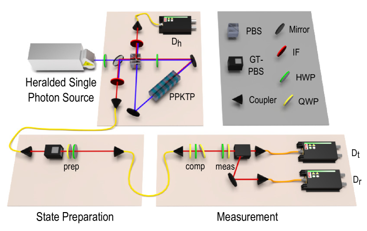
Figure 6.15: The experimental setup. Polarization-separable photon pairs are created via parametric downconversion, and detection of a photon at $D_{h}$ heralds the presence of a single photon. The polarization state of this photon is prepared with a polarizer and two waveplates (prep). A single-mode fibre is a spatial filter that decouples beam deflections caused by the state-preparation and measurement waveplates from the coupling efficiency into the detectors. Three waveplates (comp) are set to undo the polarization rotation caused by the fibre. Two waveplates (meas), a polarizing beamsplitter, and detectors $D_{r}$ and $D_{t}$ perform a two-outcome measurement on the state. PPKTP, periodically poled potassium titanyl phosphate; PBS, polarizing beamsplitter; GT-PBS, Glan-Taylor polarizing beamsplitter; IF, interference filter; HWP, half-waveplate; QWP, quarter-waveplate. Figure credit: Kevin Resch [63].

Secondary preparations in quantum theory

It is easiest to describe the details of our procedure for defining secondary preparations if we make the assumption that quantum theory correctly describes the experiment. Further on, we will describe the procedure for a generalised probabilistic theory (GPT) for this experiment.

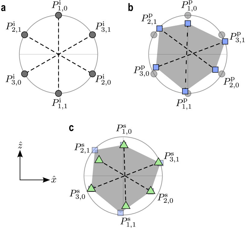
Figure 6.16: Illustration of our solution to the problem of the failure to achieve strict operational equivalences of preparations (under the simplifying assumption that these are confined to the $\hat{x}-\hat{z}$ plane of the Bloch sphere). For a given pair, $P_{t,0}$ and $P_{t,1}$, the midpoint along the line connecting the corresponding points represents their equal mixture, $P_{t}$. a. The target preparations $P^{\rm i}_{t,b}$, with the coincidence of the midpoints of the three lines illustrating that they satisfy the operational equivalence (6.60) exactly. b. Illustration of how errors in the experiment (exaggerated in magnitude) will imply that the realized preparations $P^{\rm p}_{t,b}$ (termed primary) will deviate from the ideal. The lines indicate that not only do these preparations fail to satify the operational equivalence (6.60), but since the lines do not meet, no mixtures of the $P^{\rm p}_{t,0}$ and $P^{\rm p}_{t,1}$ can be found at a single point independent of $t$. The set of preparations corresponding to probabilistic mixtures of the $P^{\rm p}_{t,b}$ are depicted by the grey region. c. Secondary preparations $P^{\rm s}_{t,b}$ have been chosen from this grey region, with the coincidence of the midpoints of the three lines indicating that the operational equivalence (6.60) has been restored. Note that we require only that the mixtures of the three pairs of preparations be the same, not that they correspond to the completely mixed state. Figure credit: Michael Mazurek and Matthew Pusey [63].

The actual preparations and measurements in the experiment, which we call the primary procedures and denote by $P^{\rm p}_{1,0}$, $P^{\rm p}_{1,1}$, $P^{\rm p}_{2,0}$, $P^{\rm p}_{2,1}$, $P^{\rm p}_{3,0}$, $P^{\rm p}_{3,1}$ and $M^{\rm p}_{1}$, $M^{\rm p}_{2}$, $M^{\rm p}_{3}$, necessarily deviate from the ideal versions and consequently their mixtures, that is, $P^{\rm p}_{1}$, $P^{\rm p}_{2}$, $P^{\rm p}_{3}$ and $M^{\rm p}_{*}$, fail to achieve strict equality in Eqs. (6.58) and (6.60).

We solve this problem as follows.

• From the outcome probabilities on the six primary preparations, one can infer the outcome probabilities on the entire family of probabilistic mixtures of these. It is possible to find within this family many sets of six preparations, $P^{\rm s}_{1,0}$, $P^{\rm s}_{1,1}$, $P^{\rm s}_{2,0}$, $P^{\rm s}_{2,1}$, $P^{\rm s}_{3,0}$, $P^{\rm s}_{3,1}$, which define mixed preparations $P^{\rm s}_{1}$, $P^{\rm s}_{2}$, $P^{\rm s}_{3}$ that satisfy the operational equivalences of Eq. (6.60) exactly. We call the $P^{\rm s}_{t,b}$ secondary preparations. We can define secondary measurements $M^{\rm s}_{1}$, $M^{\rm s}_{2}$, $M^{\rm s}_{3}$ and their uniform mixture $M^{\rm s}_{*}$ in a similar fashion. The essence of our approach, then, is to identify such secondary sets of procedures and use these to calculate $A^{\prime}$. If quantum theory is correct, then we expect to get a value of $A$ close to 1 if and only if we can find suitable secondary procedures that are close to the ideal versions.

• In Fig. 6.16, we describe the construction of secondary preparations in a simplified example of six density operators that deviate from the ideal states only within the $\hat{x}-\hat{z}$ plane of the Bloch sphere. In practice, the six density operators realized in the experiment will not quite lie in a plane. We use the same idea to contend with this, but with one refinement: we supplement our set of ideal preparations with two additional ones, denoted $P^{\rm i}_{4,0}$ and $P^{\rm i}_{4,1}$ corresponding to the two eigenstates of $\vec{\sigma}\cdot\hat{y}$. The two procedures that are actually realized in the experiment are denoted $P^{\rm p}_{4,0}$ and $P^{\rm p}_{4,1}$ and are considered supplements to the primary set. We then search for our six secondary preparations among the probabilistic mixtures of this supplemented set of primaries rather than among the probabilistic mixtures of the original set. Without this refinement, it can happen that one cannot find six secondary preparations that are close to the ideal versions.

• To see why this refinement is needed, consider the case where the six primary preparations deviate from the ideals within the bulk of the Bloch sphere. The fact that our proof only requires that the secondary preparations satisfy Eq. (6.76) means that the different pairs, $P^{\rm s}_{t,0}$ and $P^{\rm s}_{t,1}$ for $t\in\{1,2,3\}$, need not all mix to the center of the Bloch sphere, but only to the same state. It follows that the three pairs need not be coplanar in the Bloch sphere. Note, however, for any two values, $t$ and $t^{\prime}$, the four preparations $P^{\rm s}_{t,0},P^{\rm s}_{t,1},P^{\rm s}_{t^{\prime},0},P^{\rm s}_{t^{\prime},1}$ do need to be coplanar. Any mixing procedure defines a map from each of the primary preparations $P^{\rm p}_{t,b}$ to the corresponding secondary preparation $P^{\rm s}_{t,b}$, which can be visualized as a motion of the corresponding point within the Bloch sphere. To ensure that the six secondary preparations approximate well the ideal preparations while also defining mixed preparations $P^{\rm s}_{1}$, $P^{\rm s}_{2}$ and $P^{\rm s}_{3}$ that satisfy the appropriate operational equivalences, the mixing procedure must allow for motion in the $\pm\hat{y}$ direction. Consider what happens if one tries to achieve such motion without supplementing the primary set with the eigenstates of $\vec{\sigma}\cdot\hat{y}$. A given point that is biased towards $-\hat{y}$ can be moved in the $+\hat{y}$ direction by mixing it with another point that has less bias in the $-\hat{y}$ direction. However, because the primary preparations are widely separated within the $\hat{x}-\hat{z}$ plane, achieving a small motion in $+\hat{y}$ direction in this fashion comes at the price of a large motion within the $\hat{x}-\hat{z}$ plane, implying a significant motion away from the ideal. This problem is particularly pronounced if the primary points are very close to coplanar.

• The best way to move a given point in the $\pm\hat{y}$ direction is to mix it with a point that is at roughly the same location within the $\hat{x}-\hat{z}$ plane, but displaced in the $\pm\hat{y}$ direction. This scheme, however, would require supplementing the primary set with one or two additional preparations for every one of its elements. Supplementing the original set with just the two eigenstates of $\vec{\sigma}\cdot\hat{y}$ constitutes a good compromise between keeping the number of preparations low and ensuring that the secondary preparations are close to the ideal. Because the $\vec{\sigma}\cdot\hat{y}$ eigenstates have the greatest possible distance from the $\hat{x}-\hat{z}$ plane, they can be used to move any point close to that plane in the $\pm\hat{y}$ direction while generating only a modest motion within the $\hat{x}-\hat{z}$ plane.

Secondary measurements in quantum theory

Just as with the case of preparations, we solve the problem of no strict statistical equivalences for measurements by noting that from the primary set of measurements, $M^{\rm p}_{1}$, $M^{\rm p}_{2}$ and $M^{\rm p}_{3}$, one can infer the statistics of a large family of measurements, and one can find three measurements within this family, called the secondary measurements and denoted $M^{\rm s}_{1}$, $M^{\rm s}_{2}$ and $M^{\rm s}_{3}$, such that their mixture, $M^{\rm s}_{*}$, satisfies the operational equivalence of Eq. (6.58) exactly. To give the details of our approach, it is again useful to begin with the quantum description.

• Just as a density operator can be written $\rho=\frac{1}{2}(\mathbb{I}+\vec{r}\cdot\vec{\sigma})$ to define a three-dimensional Bloch vector $\vec{r}$, an effect can be written $E=\frac{1}{2}(e_{0}\mathbb{I}+\vec{e}\cdot\vec{\sigma})$ to define a four-dimensional Bloch-like vector $(e_{0},\vec{e})$, whose four components we will call the $\hat{\mathbb{I}}$, $\hat{x}$, $\hat{y}$ and $\hat{z}$ components. Note that $e_{0}={\rm tr}(E)$, while $e_{x}={\rm tr}(\vec{\sigma}\cdot\hat{x}E)$ and so forth. The eigenvalues of $E$ are expressed in terms of these components as $\frac{1}{2}(e_{o}\pm|\vec{e}|)$. Consequently, the constraint that $0\leq E\leq\mathbb{I}$ takes the form of three inequalities $0\leq e_{o}\leq 2$, $|\vec{e}|\leq e_{0}$ and $|\vec{e}|\leq 2-e_{0}$. This corresponds to the intersection of two cones. For the case $e_{y}=0$, the Bloch representation of the effect space is three-dimensional and is displayed in Fig. 6.17. When portraying binary-outcome measurements associated to a POVM $\{E,\mathbb{I}-E\}$ in this representation, it is sufficient to portray the Bloch-like vector $(e_{0},\vec{e})$ for outcome $E$ alone, given that the vector for $\mathbb{I}-E$ is simply $(2-e_{0},-\vec{e})$. Similarly, to describe any mixture of two such POVMs, it is sufficient to describe the mixture of the effects corresponding to the first outcome.

• The family of measurements that is defined in terms of the primary set is slightly different than what we had for preparations. The reason is that each primary measurement on its own generates a family of measurements by probabilistic post-processing of its outcome. If we denote the outcome of the original measurement by $X$ and that of the processed measurement by $X^{\prime}$, then the probabilistic processing is a conditional probability $p(X^{\prime}|X)$. It is sufficient to determine the convexly-extremal post-processings, since all others can be obtained from these by mixing. For the case of binary outcome measurements considered here, there are just four extremal post-processings: the identity process, $p(X^{\prime}|X)=\delta_{X^{\prime},X}$; the process that flips the outcome, $p(X^{\prime}|X)=\delta_{X^{\prime},X\oplus 1}$; the process that always generates the outcome $X^{\prime}=0$, $p(X^{\prime}|X)=\delta_{X^{\prime},0}$; and the process that always generates the outcome $X^{\prime}=1$, $p(X^{\prime}|X)=\delta_{X^{\prime},1}$. Applying these to our three primary measurements, we obtain eight measurements in all: the two that generate a fixed outcome, the three originals, and the three originals with the outcome flipped. If the set of primary measurements corresponded to the ideal set, then the eight extremal post-processings would correspond to the observables $0,\mathbb{I},\vec{\sigma}\cdot\hat{n_{1}},{-}\vec{\sigma}\cdot\hat{n_{1}},\vec{\sigma}\cdot\hat{n_{2}},{-}\vec{\sigma}\cdot\hat{n_{2}},\vec{\sigma}\cdot\hat{n_{3}},{-}\vec{\sigma}\cdot\hat{n_{3}}$. In practice, the last six measurements will be unsharp. These eight measurements can then be mixed probabilistically to define the family of measurements from which the secondary measurements must be chosen. We refer to this family as the convex hull of the post-processings of the primary set.

• Consider a simplified example wherein the primary measurements have Bloch-like vectors with vanishing component along $\hat{y}$, $e_{y}=0$, and unit component along $\mathbb{I}$, $e_{0}=1$, so that $E=\frac{1}{2}(\mathbb{I}+e_{x}\vec{\sigma}\cdot\hat{x}+e_{z}\vec{\sigma}\cdot\hat{z})$. In this case, the constraint $0\leq E\leq\mathbb{I}$ reduces to $|\vec{e}|\leq 1$, which is the same constraint that applies to density operators confined to the $\hat{x}-\hat{z}$ plane of the Bloch sphere. Here, the only deviation from the ideal is within this plane, and the construction is precisely analogous to what is depicted in Fig. 6.16.

• Unlike the case of preparations, however, the primary measurements can deviate from the ideal in the $\hat{\mathbb{I}}$ direction, that is, $E$ may have a component along $\mathbb{I}$ that deviates from $1$, which corresponds to introducing a state-independent bias on the outcome of the measurement. This is where the extremal post-processings yielding the constant-outcome measurements corresponding to the observables 0 and $\mathbb{I}$ come in. They allow one to move in the $\pm\hat{\mathbb{I}}$ direction.

  Fig. 6.17 presents an example wherein the primary measurements have Bloch-like vectors that deviate from the ideal not only within the $\hat{x}-\hat{z}$ plane, but in the $\hat{\mathbb{I}}$ direction as well (it is still presumed, however, that all components in the $\hat{y}$ direction are vanishing).

  

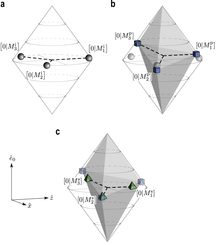
  Figure 6.17: A depiction of the construction of secondary measurements from primary ones in the simplified case where the component along $\hat{y}$ is zero. For each measurement, we specify the point corresponding to the Bloch representation of its first outcome. These are labelled $[0|M_{1}]$, $[0|M_{2}]$ and $[0|M_{3}]$. The equal mixture of these three, labelled $[0|M_{*}]$, is the centroid of these three points, i.e. the point equidistant from all three. a. The ideal measurements $[0|M^{\rm i}_{t}]$ with centroid at $\mathbb{I}/2$, illustrating that the operational equivalence (6.58) is satisfied exactly. b. Errors in the experiment (exaggerated) will imply that the realized measurements $[0|M^{\rm p}_{t,}]$ (termed primary) will deviate from the ideal, and their centroid deviates from $\mathbb{I}/2$. The family of points corresponding to probabilistic mixtures of the $[0|M^{\rm p}_{t}]$ and the observables $0$ and $\mathbb{I}$ are depicted by the grey region. (For clarity, we have not depicted the outcome-flipped versions of the three primary measurements, and have not included them in the probabilistic mixtures. As we note in the text, such a restriction still allows for a good construction.) c. The secondary measurements $M^{\rm s}_{t}$ that have been chosen from this grey region. They are chosen such that their centroid is at $\mathbb{I}/2$, restoring the operational equivalence (6.58). Figure credit: Michael Mazurek [63].

  In practice, of course, the $\hat{y}$ component of our measurements never vanishes precisely either. We therefore apply the same trick as we did for the preparations.

  We supplement the set of primary measurements with an additional measurement, denoted $M^{\rm p}_{4}$, that ideally corresponds to the observable $\vec{\sigma}\cdot\hat{y}$. The post-processing which flips the outcome then corresponds to the observable $-\vec{\sigma}\cdot\hat{y}$. Mixing the primary measurements with $M^{\rm p}_{4}$ and its outcome-flipped counterpart allows motion in the $\pm\hat{y}$ direction within the Bloch cone.

• Note that the capacity to move in both the $\hat{y}$ and the $-\hat{y}$ direction is critical for achieving the operational equivalence of Eq. (6.58), because if the secondary measurements had a common bias in the $\hat{y}$ direction, they could not mix to the POVM $\{\mathbb{I}/2,\mathbb{I}/2\}$ as Eq. (6.75) requires. For the preparations, by contrast, supplementing the primary set by just one of the eigenstates of $\vec{\sigma}\cdot\hat{y}$ would still work, given that the mixed preparations $P^{\rm s}_{t}$ do not need to coincide with the completely mixed state $\mathbb{I}/2$.

  The secondary measurements $M^{\rm s}_{1}$, $M^{\rm s}_{2}$ and $M^{\rm s}_{3}$ are then chosen from the convex hull of the post-processings of the $M^{\rm p}_{1},M^{\rm p}_{2},M^{\rm p}_{3},M^{\rm p}_{4}$. Without this supplementation, it may be impossible to find secondary measurements that define an $M^{\rm s}_{*}$ that satisfies the operational equivalences while providing a good approximation to the ideal measurements.

• In all, under the extremal post-processings of the supplemented set of primary measurements, we obtain ten points which ideally correspond to the observables $0,\mathbb{I},\vec{\sigma}\cdot\hat{n_{1}},{-}\vec{\sigma}\cdot\hat{n_{1}},\vec{\sigma}\cdot\hat{n_{2}},{-}\vec{\sigma}\cdot\hat{n_{2}},\vec{\sigma}\cdot\hat{n_{3}},{-}\vec{\sigma}\cdot\hat{n_{3}},\vec{\sigma}\cdot\hat{y}$, and ${-}\vec{\sigma}\cdot\hat{y}$. Note that the outcome-flipped versions of the three primary measurements are not critical for defining a good set of secondary measurements, and indeed we find that we can dispense with them and still obtain good results. This is illustrated in the example of Fig. 6.17.

• Note that in order to identify which density operators have been realized in an experiment, the set of measurements must be complete for state tomography. Similarly, to identify which sets of effects have been realized, the set of preparations must be complete for measurement tomography. This tomographic completeness is crucial to be able to explicitly verify the operational equivalences that a test of noncontextuality requires. However, the original ideal sets fail to be tomographically complete because they are restricted to a plane of the Bloch sphere, and an effective way to complete them is to add the observable $\vec{\sigma}\cdot\hat{y}$ to the measurements and its eigenstates to the preparations. Therefore, even if we did not already need to supplement these ideal sets for the purpose of providing greater leeway in the construction of the secondary procedures, we would be forced to do so in order to ensure that one can verify operational equivalences explicitly.

Secondary preparations and measurements in generalized probabilistic theories

To analyze our data in a manner that does not prejudice which model—noncontextual, quantum, or otherwise—does justice to it, we must search for representations of the preparations and measurements not amongst density operators and sets of effects, but rather their more abstract counterparts in the formalism of generalized probabilistic theories (GPTs) [67, 68], called generalized states and effects. The assumption that the system is a qubit is replaced by the strictly weaker assumption that three two-outcome measurements are tomographically complete. (In generalized probabilistic theories, a set of measurements is called tomographically complete if their statistics suffice to determine the state.) We take these states and effects as estimates of our primary preparations and measurements, and we define our estimate of the secondary procedures in terms of these, which in turn are used to calculate our estimate for $A^{\prime}$. We explain how the raw data is fit to a set of generalized states and effects following the procedure outlined in Section 6.7.2.

Since we do not want to presuppose that our experiment is well fit by a quantum description, we work with GPT states and effects which are inferred from the matrix $\mathbb{D}^{\rm p}$:

$$\mathbb{D}^{\rm p}=\begin{pmatrix}p^{1}_{1,0}&p^{1}_{1,1}&\cdots&p^{1}_{4,0}&p^{1}_{4,1}\\ p^{2}_{1,0}&p^{2}_{1,1}&\cdots&p^{2}_{4,0}&p^{2}_{4,1}\\ p^{3}_{1,0}&p^{3}_{1,1}&\cdots&p^{3}_{4,0}&p^{3}_{4,1}\\ p^{4}_{1,0}&p^{4}_{1,1}&\cdots&p^{4}_{4,0}&p^{4}_{4,1}\end{pmatrix}.$$ (6.96)

where

$$p^{t^{\prime}}_{t,b}\equiv p(0|M^{\rm p}_{t^{\prime}},P^{\rm p}_{t,b})$$ (6.97)

is the probability of obtaining outcome $0$ in the $t^{\prime}$th measurement that was actually realized in the experiment (recall that we term this measurement primary and denote it by $M^{\rm p}_{t^{\prime}}$), when it follows the $(t,b)$th preparation that was actually realized in the experiment (recall that we term this preparation primary and denote it by $P^{\rm p}_{t,b}$). These probabilities are estimated by fitting the raw experimental data (which are merely finite samples of the true probabilities) to a GPT. We now describe this procedure before moving on to the construction of $\mathbb{D}^{\rm s}$:

Fitting the raw data to a generalized probabilistic theory: In our experiment we perform four measurements on each of eight input states. If we define $r^{t^{\prime}}_{t,b}$ as the fraction of ‘0’ outcomes returned by measurement $M_{t^{\prime}}$ on preparation $P_{t,b}$, the results can be summarized in a $4\times 8$ matrix of raw data, $\mathbb{D}^{\rm r}$, defined as:

$$\mathbb{D}^{\rm r}=\begin{pmatrix}r^{1}_{1,0}&r^{1}_{1,1}&\cdots&r^{1}_{4,0}&r^{1}_{4,1}\\ r^{2}_{1,0}&r^{2}_{1,1}&\cdots&r^{2}_{4,0}&r^{2}_{4,1}\\ r^{3}_{1,0}&r^{3}_{1,1}&\cdots&r^{3}_{4,0}&r^{3}_{4,1}\\ r^{4}_{1,0}&r^{4}_{1,1}&\cdots&r^{4}_{4,0}&r^{4}_{4,1}\end{pmatrix}.$$ (6.98)

Each row of $\mathbb{D}^{\rm r}$ corresponds to a measurement, ordered from top to bottom as $M_{1}$, $M_{2}$, $M_{3}$, and $M_{4}$. Similary, the columns are labelled from left to right as $P_{1,0}$, $P_{1,1}$, $P_{2,0}$, $P_{2,1}$, $P_{3,0}$, $P_{3,1}$, $P_{4,0}$, and $P_{4,1}$.

In order to test the assumption that three independent binary-outcome measurements are tomographically complete for our system, we fit the raw data to a matrix, $\mathbb{D}^{\rm p}$, of primary data defined in Eq. (6.96). $\mathbb{D}^{\rm p}$ contains the outcome probabilities of four measurements on eight states in the GPT-of-best-fit to the raw data. We fit to a GPT in which three 2-outcome measurements are tomographically complete, which we characterize with the following proposition, a special case of Theorem 11:

Proposition 12.

A matrix $\mathbb{D}^{\rm p}$ can arise from a GPT in which three two-outcome measurements are tomographically complete if and (with a measure zero set of exceptions) only if $ap^{1}_{t,b}+bp^{2}_{t,b}+cp^{3}_{t,b}+dp^{4}_{t,b}-1=0$ for some real constants $\{a,b,c,d\}$.

Geometrically, the proposition dictates that the eight columns of $\mathbb{D}^{\rm p}$ lie on the 3-dimensional hyperplane defined by the constants $\{a,b,c,d\}$.

To find the GPT-of-best-fit we fit a 3-d hyperplane to the eight 4-dimensional points that make up the columns of $\mathbb{D}^{\rm r}$. We then map each column of $\mathbb{D}^{\rm r}$ to its closest point on the hyperplane, and these eight points will make up the columns of $\mathbb{D}^{\rm p}$. We use a weighted total least-squares procedure [76, 77] to perform this fit. Each element of $\mathbb{D}^{\rm r}$ has an uncertainty, $\Delta r^{t^{\prime}}_{t,b}$, which is estimated assuming the dominant source of error is the statistical error arising from Poissonian counting statistics. We define the weighted distance, $\chi_{t,b}$, between the $(t,b)$ column of $\mathbb{D}^{\rm r}$ and $\mathbb{D}^{\rm p}$ as $\chi_{t,b}=\sqrt{\sum_{t^{\prime}=1}^{4}\left(r^{t^{\prime}}_{t,b}-p^{t^{\prime}}_{t,b}\right)^{2}/\left(\Delta r^{t^{\prime}}_{t,b}\right)^{2}}$. Finding the best-fitting hyperplane can be summarized as the following minimization problem:

$$\underset{\{p^{i}_{t,b},a,b,c,d\}}{\text{minimize}} \chi^{2}=\sum_{t=1}^{4}\sum_{b=0}^{1}\chi_{t,b}^{2},$$ (6.99)

subject to $$ap^{1}_{t,b}+bp^{2}_{t,b}+cp^{3}_{t,b}+dp^{4}_{t,b}-1=0$$

$$\forall\,t=1,\ldots,4,b=0,1.$$

The optimization problem as currently phrased is a problem in 36 variables—the 32 elements of $\mathbb{D}^{\rm p}$ together with the hyperplane parameters $\{a,b,c,d\}$. We can simplify this by first solving the simpler problem of finding the weighted distance $\chi_{t,b}$ between the $(t,b)$ column of $\mathbb{D}^{\rm r}$ and the hyperplane $\{a,b,c,d\}$. This can be phrased as the following 8-variable optimization problem:

$$\underset{\{p^{1}_{t,b},p^{2}_{t,b},p^{3}_{t,b},p^{4}_{t,b}\}}{\text{minimize}} \chi_{t,b}^{2}=\sum_{t^{\prime}=1}^{4}\frac{(r^{t^{\prime}}_{t,b}-p^{t^{\prime}}_{t,b})^{2}}{\left(\Delta r^{t^{\prime}}_{t,b}\right)^{2}},$$ (6.100)

subject to $$ap^{1}_{t,b}+bp^{2}_{t,b}+cp^{3}_{t,b}+dp^{4}_{t,b}-1=0.$$

Using the method of Lagrange multipliers [76], we define the Lagrange function $\Gamma=\chi_{t,b}^{2}+\gamma(ap^{1}_{t,b}+bp^{2}_{t,b}+cp^{3}_{t,b}+dp^{4}_{t,b}-1)$, where $\gamma$ denotes the Lagrange multiplier, then simultaneously solve

$$\frac{\partial\Gamma}{\partial\gamma}=0$$ (6.101)

and

$$\frac{\partial\Gamma}{\partial p^{t^{\prime}}_{t,b}}=0,\;t^{\prime}=1,\ldots,4$$ (6.102)

for the variables $\gamma$, $p^{1}_{t,b}$, $p^{2}_{t,b}$, $p^{3}_{t,b}$, and $p^{4}_{t,b}$. Substituting the solutions for $p^{1}_{t,b}$, $p^{2}_{t,b}$, $p^{3}_{t,b}$ and $p^{4}_{t,b}$ into Eq. (LABEL:eq:chi_j) we find

$$\chi_{t,b}^{2}=\frac{(ar^{1}_{t,b}+br^{2}_{t,b}+cr^{3}_{t,b}+dr^{4}_{t,b}-1)^{2}}{\left(a\Delta r^{1}_{t,b}\right)^{2}+\left(b\Delta r^{2}_{t,b}\right)^{2}+\left(c\Delta r^{3}_{t,b}\right)^{2}+\left(d\Delta r^{4}_{t,b}\right)^{2}},$$ (6.103)

which now only contains the variables $a$, $b$, $c$, and $d$.

The hyperplane-finding problem can now be stated as the following four-variable optimization problem:

$$\underset{\{a,b,c,d\}}{\text{minimize}} \chi^{2}=\sum_{t=1}^{4}\sum_{b=0}^{1}\chi_{t,b}^{2}$$ (6.104)

which we solve numerically.

The $\chi^{2}$ parameter returned by the fitting procedure is a measure of the goodness-of-fit of the hyperplane to the data. Since we are fitting eight datapoints to a hyperplane defined by four fitting parameters $\{a,b,c,d\}$, we expect the $\chi^{2}$ parameter to be drawn from a $\chi^{2}$ distribution with four degrees of freedom [77], which has a mean of 4. The experiment was run 100 times and 100 independent $\chi^{2}$ parameters were obtained; these were found to have a mean of $3.9\pm 0.3$ [63]. In addition a more stringent test of the fit of the model to the data was performed by summing the counts from all 100 experimental runs before performing a single fit. This fit returns a $\chi^{2}$ of 4.33, which has a $p$-value of 36%. The outcomes of these tests are consistent with our assumption that the raw data can be explained by a GPT in which three 2-outcome measurements are tomographically complete and which also exhibits Poissonian counting statistics. Had the fitting procedure returned $\chi^{2}$ values that were much higher, this might have indicated that the theoretical description of the preparation and measurement procedures required more than three degrees of freedom. On the other hand, had the fitting returned an average $\chi^{2}$ much lower than 4, this could have indicated that we had overestimated the amount of uncertainty in our data.

After finding the hyperplane-of-best-fit $\left\{a,b,c,d\right\}$, we find the points on the hyperplane that are closest to each column of $\mathbb{D}^{\rm r}$. This is done by numerically solving for $p^{1}_{t,b}$, $p^{2}_{t,b}$, $p^{3}_{t,b}$, and $p^{4}_{t,b}$ in (LABEL:eq:chi_j) for each value of $(t,b)$. The point on the hyperplane closest to the $(t,b)$ column of $\mathbb{D}^{\rm r}$ becomes the $(t,b)$ column of $\mathbb{D}^{\rm p}$. The matrix $\mathbb{D}^{\rm p}$ is then used to find the secondary preparations and measurements.

Inferring the secondary data matrix $\mathbb{D}^{\rm s}$: The rows of the $\mathbb{D}^{\rm p}$ matrix define the GPT effects. We denote the vector defined by the $t$th row, which is associated to the measurement event $[0|M_{t}^{\rm p}]$ (obtaining the 0 outcome in the primary measurement $M_{t}^{\rm p}$), by $\mathbf{M}_{t}^{\rm p}$. Similarly, the columns of this matrix define the GPT states. We denote the vector associated to the $(t,b)$th column, which is associated to the primary preparation $P^{\rm p}_{t,b}$, by $\mathbf{P}^{\rm p}_{t,b}$.

As we outlined in the previous section, we define the secondary preparation $P^{\rm s}_{t,b}$ by a probabilistic mixture of the primary preparations. Thus, the GPT state of the secondary preparation is a vector $\mathbf{P}^{\rm s}_{t,b}$ that is a probabilistic mixture of the $\mathbf{P}^{\rm p}_{t,b}$,

$$\mathbf{P}^{\rm s}_{t,b}=\sum_{t^{\prime}=1}^{4}\sum_{b^{\prime}=0}^{1}u_{t^{\prime},b^{\prime}}^{t,b}\mathbf{P}_{t^{\prime},b^{\prime}}^{\rm p},$$ (6.105)

where the $u_{t^{\prime},b^{\prime}}^{t,b}$ are the weights in the mixture.

A secondary measurement $M_{t^{\prime}}^{\rm s}$ is obtained from the primary measurements in a similar fashion, but in addition to probabilistic mixtures, one must allow certain post-processings of the measurements, in analogy to the quantum case described above.

The set of all post-processings of the primary outcome-0 measurement events has extremal elements consisting of the outcome-0 measurement events themselves together with: the measurement event that always occurs (i.e. always obtaining outcome ‘0’), which is represented by the vector of probabilities where every entry is 1, denoted $\mathbf{1}$; the measurement event that never occurs (i.e. never obtaining outcome ‘0’ or always obtaining outcome ‘1’), which is represented by the vector of probabilities where every entry is 0, denoted $\mathbf{0}$; and the outcome-1 measurement events, $[1|M_{t}^{\rm p}]$, represented by the vector $\mathbf{1}-\mathbf{M}_{t}^{\rm p}$.

We can therefore define our three secondary outcome-0 measurement events as probabilistic mixtures of the four primary ones as well as the extremal post-processings mentioned above, that is

$$\mathbf{M}_{t}^{\rm s}=\sum_{t^{\prime}=1}^{4}v_{t^{\prime}}^{t}\mathbf{M}_{t^{\prime}}^{\rm p}+v_{\mathbf{0}}^{t}\mathbf{0}+v_{\mathbf{1}}^{t}\mathbf{1}+\sum_{t^{\prime\prime}=1}^{4}v_{\lnot t^{\prime\prime}}^{t}(\mathbf{1}-\mathbf{M}_{t^{\prime\prime}}^{\rm p}),$$ (6.106)

where for each $t$, the vector of weights in the mixture is $(v_{1}^{t},v_{2}^{t},v_{3}^{t},v_{4}^{t},v_{\mathbf{0}}^{t},v_{\mathbf{1}}^{t},v_{\lnot 1}^{t},v_{\lnot 2}^{t},v_{\lnot 3}^{t},v_{\lnot 4}^{t})$. We see that this is a particular type of linear transformation on the rows.

Again, as mentioned in the discussion of the quantum case, we can in fact limit the post-processing to exclude the outcome-1 measurement events for $M_{1}$, $M_{2}$ and $M_{3}$, keeping only the outcome-1 event for $M_{4}$, and still obtain good results. Thus we found it sufficient to search for secondary outcome-0 measurement events among those of the form

$$\mathbf{M}_{t}^{\rm s}=\sum_{t^{\prime}=1}^{4}v_{t^{\prime}}^{t}\mathbf{M}_{t^{\prime}}^{\rm p}+v_{\mathbf{0}}^{t}\mathbf{0}+v_{\mathbf{1}}^{t}\mathbf{1}+v_{\lnot 4}^{t}(\mathbf{1}-\mathbf{M}_{4}^{\rm p}),$$ (6.107)

where for each $t$, the vector of weights in the mixture is $(v_{1}^{t},v_{2}^{t},v_{3}^{t},v_{4}^{t},v_{\mathbf{0}}^{t},v_{\mathbf{1}}^{t},v_{\lnot 4}^{t})$.

Returning to the preparations, we choose the weights $u^{t,b}_{t^{\prime},b^{\prime}}$ to maximize the function

$$C_{\rm P}\equiv\frac{1}{6}\sum_{t=1}^{3}\sum_{b=0}^{1}u_{t,b}^{t,b}$$ (6.108)

subject to the linear constraint

$$\frac{1}{2}\sum_{b}\mathbf{P}^{\rm s}_{1,b}=\frac{1}{2}\sum_{b}\mathbf{P}^{\rm s}_{2,b}=\frac{1}{2}\sum_{b}\mathbf{P}^{\rm s}_{3,b}.$$ (6.109)

This optimization ensures that the secondary preparations are as close as possible to the primary ones while ensuring that they satisfy the relevant operational equivalences exactly. For the experiment of Ref. [63], the reported $C_{\rm P}=0.9969\pm 0.0001$, indicating that the secondary preparations are indeed very close to the primary ones.

The scheme for finding the weights $(v_{1}^{t},v_{2}^{t},v_{3}^{t},v_{4}^{t},v_{\mathbf{0}}^{t},v_{\mathbf{1}}^{t},v_{\lnot 4}^{t})$ that define the secondary measurements is analogous. Using a linear program, we find the vector of such weights that maximizes the function

$$C_{\rm M}\equiv\frac{1}{3}\sum_{t=1}^{3}v_{t}^{t},$$ (6.110)

subject to the constraint that

$$\mathbf{M}_{*}^{\rm s}=\frac{1}{2}\mathbf{1},$$ (6.111)

where $\mathbf{M}_{*}^{\rm s}\equiv\frac{1}{3}\sum_{t=1}^{3}\mathbf{M}_{t}^{\rm s}$. A high value of $C_{\mathrm{M}}$ signals that each of the three secondary measurements is close to the corresponding primary one. The experiment of Ref. [63] reported $C_{\rm M}=0.9976\pm 0.0001$, again indicating the closeness of the secondary measurements to the primary ones.

This optimization defines the precise linear transformation of the rows of $\mathbb{D}^{\rm p}$ and the linear transformation of the columns of $\mathbb{D}^{\rm p}$ that serve to define the secondary preparations and measurements. By combining the operations on the rows and on the columns, we obtain from $\mathbb{D}^{\rm p}$ a $3\times 6$ matrix, denoted $\mathbb{D}^{\rm s}$, whose entries $s^{t^{\prime}}_{t,b}$ are

$$\sum_{\tau=1}^{4}\sum_{\beta=0}^{1}u^{t,b}_{\tau,\beta}\left[\sum_{\tau^{\prime}=1}^{4}v^{t^{\prime}}_{\tau^{\prime}}p^{\tau^{\prime}}_{\tau,\beta}+v^{t^{\prime}}_{\mathbf{0}}0+v^{t^{\prime}}_{\mathbf{1}}1+v^{t^{\prime}}_{\lnot 4}(1-p^{4}_{\tau,\beta})\right]$$ (6.112)

where $t^{\prime},t\in\{1,2,3\}$, $b\in\{0,1\}$. This matrix describes the secondary preparations $P_{t,b}^{\rm s}$ and measurements $M_{t^{\prime}}^{\rm s}$. The component $s^{t^{\prime}}_{t,b}$ of this matrix describes the probability of obtaining outcome 0 in measurement $M^{\rm s}_{t^{\prime}}$ on preparation $P^{\rm s}_{t,b}$, that is,

$$s^{t^{\prime}}_{t,b}\equiv p(0|M^{\rm s}_{t^{\prime}},P^{\rm s}_{t,b}).$$ (6.113)

These probabilities are the ones that are used to calculate the value of $A^{\prime}$ via Eq.(6.62). The value of $A^{\prime}$ reported in the experiment was $A^{\prime}=0.99709\pm 0.00007$, well above the noncontextual bound of $5/6\approx 0.833$ [63].

6.8 Chapter summary

We have shown how to contend with the problem of noisy measurements and inexact operational equivalences in tests of noncontextuality. As we explained, the methods used to derive the noncontextuality inequality motivated by the 18 ray Kochen-Specker construction can be used to derive such tests of noncontextuality from other KS-uncolourable hypergraphs as well. We also reported and generalized the methods adopted in the experimental test of the FCF inequality in hopes that such a generalization will be useful in future experimental tests of noncontextuality. An open challenge that remains is to put the assumption of tomographic completeness of a finite set of preparations and measurements on a surer footing, akin to the assumption of no-signalling in Bell tests.

Chapter 7 Back to Specker’s scenario: a theory-independent analysis

In this chapter we return to the problem of contextuality in Specker’s scenario that we first discussed in Chapter 2. In Chapter 2, we considered the LSW inequality [29] which presumes the validity of quantum theory, even though it does not assume outcome determinism for unsharp measurements. Following the development towards theory-independent tests of contextuality in the previous chapter, we will carry out this exercise for the case of Specker’s scenario in this chapter. Indeed, while the previous chapter showed how to derive robust noncontextuality inequalities from so-called “state-independent” proofs of the Kochen-Specker theorem (based on KS-uncolourability), the present chapter achieves this for “state-dependent” proofs of contextuality.

The operational noncontextuality inequalities derived in this chapter do not rely on the assumption that measurement outcomes are fixed deterministically by the ontic state of the system. They constitute a proper operational generalization of the LSW inequality discussed in Chapter 2, explicitly taking into account the lack of perfect predictability of measurement outcomes in realistic experiments. We construct quantum violations of these inequalities.

In deriving these inequalities, no assumption of the validity of quantum theory is made. An experimental violation of them would serve as a genuine test of nonclassicality which any operationally motivated theory of physics—in particular, any future modification of quantum theory—would have to accommodate. The most basic of these inequalities applies to the case of Specker’s scenario which involves three two-outcome measurements, every pair of which is jointly measured. Specker’s scenario is the minimal scenario in which contextuality with respect to joint measurement contexts can be expected to manifest itself and our analysis provides a robust noncontextuality inequality for this scenario before moving on to more general $n$-cycle scenarios.

This chapter is based on joint work with Rob Spekkens.

7.1 Introduction

Specker’s scenario was first described by Ernst Specker in the form of a parable [28, 29], a rendition of which (due to Liang, Spekkens, and Wiseman [29]) is reproduced below:

At the Assyrian School of Prophets in Arba’ilu in the time of King Asarhaddon [(681-669 BCE)], there taught a seer from Nineva. He was a distinguished representative of his faculty (eclipses of the sun and moon) and aside from the heavenly bodies, his interest was almost exclusively in his daughter. His teaching success was limited; the subject proved to be dry and required a previous knowledge of mathematics which was scarcely available. If he did not find the student interest which he desired in class, he did find it elsewhere in overwhelming measure. His daughter had hardly reached a marriageable age when he was flooded with requests for her hand from students and young graduates. And though he did not believe that he would always have her by his side, she was in any case still too young and her suitors in no way worthy. In order that the suitors might convince themselves of their unworthiness, he promised them that she would be wed to the one who could solve a prediction task that was posed to them. Each suitor was taken before a table on which three little boxes stood in a row, [each of which might or might not contain a gem], and was asked to predict which of the boxes contained a gem and which did not. But no matter how many times they tried, it seemed impossible to succeed in this task. After each suitor had made his prediction, he was ordered by the father to open any two boxes which he had predicted to be both empty or any two boxes which he had predicted to be both full [in accordance with whether he had predicted there to be at most one gem among the three boxes, or at least two gems, respectively]. But it always turned out that one contained a gem and the other one did not, and furthermore the stone was sometimes in the first and sometimes in the second of the boxes that were opened. But how can it be possible, given three boxes, to neither be able to pick out two as empty nor two as full? The daughter would have remained unmarried until the father’s death, if not for the fact that, after the prediction of the son of a prophet [whom she fancied], she quickly opened two boxes herself, one of which had been indicated to be full and the other empty, and the suitor’s prediction [for these two boxes] was found, in this case, to be correct. Following the weak protest of her father that he had wanted two other boxes opened, she tried to open the third. But this proved impossible whereupon the father grudgingly admitted that the prediction, being unfalsified, was valid. [The daughter and the suitor were married and lived happily ever after.]

In summary, Specker’s scenario involves three boxes, each of which either contains a gem or is empty, such that any two boxes can be opened together but all three boxes can’t be opened at once. Each suitor seeking to marry the seer’s daughter is asked to predict the occupancy of the three boxes, after which the seer asks him to open two boxes predicted to be both empty or both full. Upon opening two such boxes it is always found that one contains a gem and the other does not. Furthermore, the gem is sometimes found in the first box and sometimes in the second box that was opened. These correlations were described as the ‘over-protective seer’ (OS) correlations in Ref. [29]:

$$\forall i\neq j: p(X_{i}=0,X_{j}=1|M_{ij};P_{*})=\frac{1}{2}$$ (7.1)

$$p(X_{i}=1,X_{j}=0|M_{ij};P_{*})=\frac{1}{2},$$

where $i,j\in\{1,2,3\}$ label the three boxes, $M_{ij}$ denotes the operation of opening two boxes $i$ and $j$ together while $X_{i}$ and $X_{j}$ denote their respective occupancy ($0$ for no gem and $1$ for a gem), and $P_{*}$ denotes the preparation of the three boxes which yields OS correlations. Clearly, it is always the case that upon opening two boxes $i$ and $j$ one contains a gem and the other does not: $p(X_{i}\neq X_{j}|M_{ij};P_{*})=1,\forall i\neq j$.

As we did in Chapter 2, we will soon formalize this scenario in terms of performing two-outcome measurements (instead of opening boxes) and observing their outcome (instead of occupancy of the opened boxes). For now, note that observing OS correlations is surprising only if, besides the assumption that the probability of occupancy of a given box is independent of which other box it is opened with (this is essentially measurement noncontextuality), one has also made the assumption of outcome-determinism: that the occupancy of each box is fixed deterministically by some mechanism. On relaxing the assumption of outcome-determinism, the OS correlations should not be surprising: they merely say that upon opening any two boxes, a fair coin flip decides which of them contains a gem and which one doesn’t. This is consistent with the fact that the (marginalized) occupancy of each box is uniformly random. On the other hand, the OS correlations would be surprising if there are operational reasons implying that the occupancy of each box was decided deterministically, or at least with some bias, at the ontological level. Such operational reasons amount to observing high predictability of the individual measurements for an appropriate set of preparations of the boxes. This intuitive tradeoff between the observed anticorrelation and the predictability of occupancy of each box is what we formalize in our noncontextuality inequality for Specker’s scenario: a high probability of anticorrelation implies a low predictability of occupancy.

The modern rendition of this parable in Ref. [29] made it precise in terms of joint measurements of POVMs for which such joint measurability relations —pairwise joint measurements but no triplewise joint measurements—are possible. The LSW inequality formulated for qubit POVMs in Ref. [29] provided a necessary criterion for deciding whether the statistics of the pairwise joint measurements of the POVMs is consistent with a noncontextual model of quantum theory. It was conjectured that this is always the case [29]. However, as we showed in Chapter 2, this is not the case and that there exist qubit POVMs for which the LSW inequality can be violated. Such a violation has been claimed to be experimentally demonstrated recently in an experiment using the polarization of single photons [72].

A further feature that was appreciated only after the results of Refs. [29, 30] is the following: there exist three two-outcome qubit POVMs such that all three are jointly measurable, yet they admit pairwise joint measurements which cannot be obtained from the marginalization of any triplewise joint measurement. This was first noticed in Ref. [45] and later analyzed in more detail in Ref. [46]. This means that the narrative of Specker’s parable changes in the following way to accomodate this quantum feature: it is no longer necessary that the three boxes can’t be opened together. Rather, even if the three boxes could be opened together, it may still be that opening the boxes pairwise leads to statistics which cannot arise from opening all three of them together. In view of this, we will relax the requirement that the three qubit POVMs be triplewise incompatible since it turns out not to be necessary to witness contextuality.

Much as Refs. [29, 30, 46] clarified the impossibility of explaining statistics of qubit POVMs in a noncontextual model, they left open the question of whether it is possible to make a theory-independent claim regarding contextuality in this scenario. We address this deficiency of earlier analyses by deriving noncontextuality inequalities that apply to any operational theory that might govern the experimental statistics. Notice that Specker’s scenario is the minimal scenario in which contextuality with respect to joint measurement contexts can be manifested: at least three measurements are needed for distinct joint measurement contexts for a given measurement to be defined and every pair of these measurements has to be jointly measurable for a scenario where contextuality can be expected. Furthermore, two-outcome measurements are the simplest possible ones.

7.2 Specker’s scenario

7.2.1 Noncontextuality inequalities for Specker’s scenario

We consider three two-outcome measurements, $\{M_{1},M_{2},M_{3}\}$, each $M_{i}$ with outcomes labelled by $X_{i}\in\{0,1\}$, such that every pair, that is, $\{M_{i},M_{j}\}$ for $(ij)\in\{(12),(23),(31)\}$, admits of a joint measurement, denoted by $M_{ij}$. $M_{ij}$ is a measurement procedure—with four outcomes denoted by $(X_{i},X_{j})$—whose measurement statistics can be coarse-grained to obtain the measurement statistics of both $M_{i}$ and $M_{j}$ for any preparation $P\in\mathcal{P}$:

$$p(X_{i}|M_{i},P) \equiv \sum_{X_{j}}p(X_{i},X_{j}|M_{ij},P),$$

$$p(X_{j}|M_{j},P) \equiv \sum_{X_{i}}p(X_{i},X_{j}|M_{ij},P).$$ (7.2)

Denoting by $M_{i}^{(j)}$ $(M_{j}^{(i)})$ the coarse-graining over $X_{j}$ $(X_{i})$ of $M_{ij}$, pairwise joint measurability of $M_{1}$, $M_{2}$ and $M_{3}$ implies these operational equivalences:

$$M_{1}^{(2)} \simeq M_{1}^{(3)}\simeq M_{1},$$

$$M_{2}^{(1)} \simeq M_{2}^{(3)}\simeq M_{2},$$

$$M_{3}^{(1)} \simeq M_{3}^{(2)}\simeq M_{3}.$$ (7.3)

We now define a measurement $M_{*}$ as follows: sample $(ij)\in\{(12),(23),(31)\}$ with probability 1/3 each and then implement $M_{ij}$ and record $(X_{i},X_{j})$. We are interested in the probability of recording anticorrelated outcomes,

$$p(\text{anti}|M_{*},P) \equiv\frac{1}{3}\sum_{(ij)}p(X_{i}\neq X_{j}|M_{ij},P).$$ (7.4)

Similarly, we consider another set of measurements, $\{M^{\prime}_{12},M^{\prime}_{23},M^{\prime}_{31}\}$, which also achieve a joint measurement of the respective pairs:

$$M_{1}^{\prime(2)} \simeq M_{1}^{\prime(3)}\simeq M_{1},$$

$$M_{2}^{\prime(1)} \simeq M_{2}^{\prime(3)}\simeq M_{2},$$

$$M_{3}^{\prime(1)} \simeq M_{3}^{\prime(2)}\simeq M_{3}.$$ (7.5)

We also define a measurement procedure $M^{\prime}_{*}$ implementing $M^{\prime}_{12}$, $M^{\prime}_{23}$, or $M^{\prime}_{31}$ with equal probabilities such that $p(\text{anti}|M^{\prime}_{*},P)$ is the probability of obtaining anticorrelated outcomes for $M^{\prime}_{*}$.

We define predictability of $(M,P)$:

$$\eta(M,P)\equiv 2\max_{X\in\{0,1\}}p(X|M,P)-1,$$ (7.6)

where $\eta(M,P)$ is a measure of how predictable, or far away from uniformly random, the distribution over outcomes is for a two-outcome measurement $M$ performed following a preparation $P$ on a system.

Let $P_{*}$, $P_{*}^{\perp}$, $P_{1}$, $P_{1}^{\perp}$, $P_{2}$, $P_{2}^{\perp}$, $P_{3}$, $P_{3}^{\perp}$ be preparation procedures, and let $P^{\rm(ave)}_{x}$ be the preparation procedure obtained by implementing $P_{x}$ with probability $1/2$ and $P_{x}^{\perp}$ with probability $1/2$ for $x\in\{1,2,3,*\}$. We suppose that the following operational equivalences among the preparations hold:

$$P^{\rm(ave)}_{*}\simeq P^{\rm(ave)}_{1}\simeq P^{\rm(ave)}_{2}\simeq P^{\rm(ave)}_{3}.$$ (7.7)

We can now state our noncontextuality inequalities for Specker’s scenario:

Theorem 13.

An operational theory which satisfies the operational equivalences of Eqs. (7.2.1), (7.2.1), and (7.7), and admits a noncontextual ontological model must necessarily satisfy the following noncontextuality inequality in Specker’s scenario:

$$p({\rm anti}|M_{*},P_{*})+p({\rm anti}|M^{\prime}_{*},P_{*}^{\perp})$$

$$\leq 2\left(1-\frac{1}{3}\eta_{\rm ave}\right),$$ (7.8)

where

$$\eta_{\rm ave}\equiv\frac{1}{6}\sum_{i=1}^{3}\left(\eta(M_{i},P_{i})+\eta(M_{i},P^{\perp}_{i})\right).$$ (7.9)

On the other hand, using only the operational equivalences of Eqs. (7.2.1) and (7.7), such an operational theory must also satisfy:

$$p({\rm anti}|M_{*},P_{*})+p({\rm anti}|M_{*},P^{\perp}_{*})\leq 2\left(1-\frac{1}{3}\eta_{\rm ave}\right),$$ (7.10)

and

$$p({\rm anti}|M_{*},P_{*})$$

$$\leq\frac{2}{3}\left(2-\eta_{\rm ave}\right).$$ (7.11)

The proof can be found in the Appendix to this chapter. The upper bound in Eqs. (13) and (7.10) is nontrivial for all values of $\eta_{\rm ave}>0$ while the upper bound in Eq. (13) is nontrivial only for values of $\eta_{\rm ave}>\frac{1}{2}$. When $\eta_{\rm ave}>\frac{1}{2}$, Eq. (13) requires fewer measurement and preparation procedures than Eqs. (13) and (7.10) in order to refute noncontextuality. Eq. (7.10) in turn requires fewer measurement procedures to be implemented than Eq. (13).

An analysis of Specker’s scenario according to KS-noncontextuality would require that the probability of anticorrelation is bounded above by $2/3$ for both $M_{*}$ and $M^{\prime}_{*}$, so that $p({\rm anti}|M_{*},P)+p({\rm anti}|M^{\prime}_{*},P^{\perp})\leq 4/3$. Similarly, in such an analysis, $p({\rm anti}|M_{*},P_{*})+p({\rm anti}|M_{*},P^{\perp}_{*})\leq 4/3$. But from Theorem 13 it is clear that these inequalities are not warranted by the assumption of noncontextuality alone. The noncontextual bound of $4/3$ will hold if and only if one has verified that $\eta(M_{i},P_{i})=\eta(M_{i},P^{\perp}_{i})=1$ for all $M_{i},P_{i},P^{\perp}_{i}$, $i\in\{1,2,3\}$. That is, when each measurement $M_{i}$ produces deterministic outcomes on both preparations $P_{i}$ and $P^{\perp}_{i}$. In this case, $\eta_{\rm ave}=1$. At the other extreme, if each $M_{i}$ has no dependence on the corresponding preparation procedures $P_{i}$ and $P_{i}^{\perp}$, so that $\eta(M_{i},P_{i})=\eta(M_{i},P_{i}^{\perp})=0$, and therefore $\eta_{\rm ave}=0$, then a noncontextual model can achieve perfect anticorrelation. A mere observation of perfect anticorrelation on its own, therefore, is not enough to demonstrate contextuality: one also needs to check that the average predictability is sufficiently large: $\eta_{\rm ave}>0$ for Eqs. (13), (7.10), and $\eta_{\rm ave}>\frac{1}{2}$ for Eq. (13). Our noncontextuality inequalities in Eqs. (13), (7.10), and (13) imply a quantitative tradeoff between operational quantities: the anticorrelation achievable in an operational theory admitting a noncontextual ontological model and the predictabilities of the measurements involved with respect to various preparations on which they are carried out.

We will see that in operational quantum theory the noncontextuality inequality of Eq. (13) can be violated. It follows that if operational quantum theory correctly describes our experiments and one can devise an experiment that is sufficiently precise that it can approach the violation predicted by quantum theory, then this experiment should yield a violation of the noncontextuality inequality. Moreover, if such an experiment is performed and the violation is observed, then this observation rules out the existence of a noncontextual ontological model regardless of the validity of operational quantum theory. Hence the result is theory-independent.

We leave open the question of whether a quantum violation exists for the noncontextuality inequalities of Eqs. (7.10) and (13). Our construction for the quantum violation of Eq. (13) does not suggest such a violation. Our noncontextuality inequalities of Eqs. (13), (7.10), and (13), are a proper operational generalization of the LSW inequality which was first obtained in Ref. [29] and for which a quantum violation was first theoretically predicted in Ref. [30] followed by an experimental demonstration of this in Ref. [72]. While the LSW inequality holds for noncontextual models of operational quantum theory, where outcome-determinism for projective measurements can be justified from preparation noncontextuality, our noncontextuality inequalities apply to arbitrary operational theories.

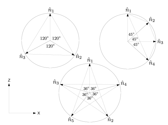
Figure 7.1: Choice of measurement directions for $n=3,4,5$.

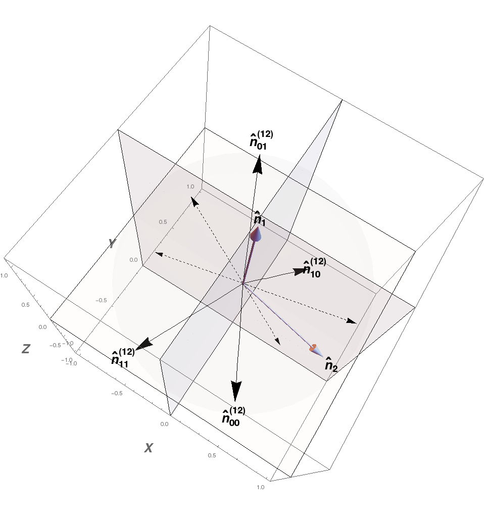
Figure 7.2: Choice of joint POVM directions for $\hat{n}_{1}$ and $\hat{n}_{2}$ in Specker’s scenario ($n=3$), $\eta_{0}=0.4566$.

7.2.2 Quantum violation of a noncontextuality inequality in Specker’s scenario

Inspired by the construction we presented in Chapter 2 (following Ref. [30]), we show the quantum violation of Eq. (13). We take $\{M_{1},M_{2},M_{3}\}$ to be three qubit measurements in an equatorial plane of the Bloch sphere, say the $ZX$ plane, such that they are pairwise jointly measurable. $M_{i}$ is associated with the qubit POVM $\{E^{(i)}_{0},E^{(i)}_{1}\}$, given by:

$$E^{(i)}_{X_{i}}\equiv\frac{1}{2}I+(-1)^{X_{i}}\frac{1}{2}\eta_{0}\vec{\sigma}\cdot\hat{n}_{i},$$ (7.12)

where $\hat{n}_{i}$ is the measurement direction, $\vec{\sigma}\equiv(\sigma_{x},\sigma_{y},\sigma_{z})$ is the vector of qubit Pauli matrices, and $I$ is the identity matrix:

$$\sigma_{x}=\left(\begin{matrix}0&1\\ 1&0\end{matrix}\right),\sigma_{y}=\left(\begin{matrix}0&-i\\ i&0\end{matrix}\right),\sigma_{z}=\left(\begin{matrix}1&0\\ 0&-1\end{matrix}\right),I=\left(\begin{matrix}1&0\\ 0&1\end{matrix}\right).$$

The necessary and sufficient condition for pairwise joint measurability of $\{M_{1},M_{2},M_{3}\}$ [30, 44, 43] is

$$\eta_{0}\leq\min_{(i,j)}\frac{1}{\sqrt{1+\sqrt{1-(\hat{n}_{i}\cdot\hat{n}_{j})^{2}}}}.$$ (7.13)

We consider two sets of pairwise joint measurements denoted by $\{M_{12},M_{23},M_{31}\}$ and $\{M^{\prime}_{12},M^{\prime}_{23},M^{\prime}_{31}\}$, where $M_{ij}$ is associated with the qubit POVM $\{E^{(ij)}_{00},E^{(ij)}_{01},E^{(ij)}_{10},E^{(ij)}_{11}\}$ and $M^{\prime}_{ij}$ is associated with the qubit POVM $\{E^{\prime(ij)}_{00},E^{\prime(ij)}_{01},E^{\prime(ij)}_{10},E^{\prime(ij)}_{11}\}$. These are given by:

$$E^{(ij)}_{X_{i}X_{j}}\equiv\frac{1}{2}\left(1+(-1)^{X_{i}+X_{j}}\eta_{0}^{2}\hat{n}_{i}.\hat{n}_{j}\right)\Pi_{\hat{n}^{ij}_{X_{i}X_{j}}}$$ (7.14)

where

$$\Pi_{\hat{n}^{ij}_{X_{i}X_{j}}}\equiv\frac{1}{2}(I+\vec{\sigma}.\hat{n}^{ij}_{X_{i}X_{j}}),$$

$$\hat{n}^{ij}_{X_{i}X_{j}}\equiv\frac{\eta_{0}((-1)^{X_{i}}\hat{n}_{i}+(-1)^{X_{j}}\hat{n}_{j})-(-1)^{X_{i}+X_{j}}\vec{a}_{ij}}{1+(-1)^{X_{i}+X_{j}}\eta_{0}^{2}\hat{n}_{i}.\hat{n}_{j}},$$

and

$$E^{\prime(ij)}_{X_{i}X_{j}}\equiv\frac{1}{2}\left(1+(-1)^{X_{i}+X_{j}}\eta_{0}^{2}\hat{n}_{i}.\hat{n}_{j}\right)\Pi_{\hat{n}^{\prime ij}_{X_{i}X_{j}}}$$ (7.15)

where

$$\Pi_{\hat{n}^{\prime ij}_{X_{i}X_{j}}}\equiv\frac{1}{2}(I+\vec{\sigma}.\hat{n}^{\prime ij}_{X_{i}X_{j}}),$$

$$\hat{n}^{\prime ij}_{X_{i}X_{j}}\equiv\frac{\eta_{0}((-1)^{X_{i}}\hat{n}_{i}+(-1)^{X_{j}}\hat{n}_{j})+(-1)^{X_{i}+X_{j}}\vec{a}_{ij}}{1+(-1)^{X_{i}+X_{j}}\eta_{0}^{2}\hat{n}_{i}.\hat{n}_{j}},$$

and

$$\vec{a}_{ij}\equiv(0,\sqrt{1+\eta_{0}^{4}(\hat{n}_{i}.\hat{n}_{j})^{2}-2\eta_{0}^{2}},0).$$

It is easy to verify that the operational equivalences of Eqs. (7.2.1) and (7.2.1) hold for this choice of pairwise joint measurements. Let $P_{x}$ and $P^{\perp}_{x}$ be the preparation procedures associated respectively with

$$\rho_{x}\equiv\frac{1}{2}I+\frac{1}{2}\vec{\sigma}\cdot\hat{n}_{x}=|+\hat{n}_{x}\rangle\langle+\hat{n}_{x}|,$$

and

$$\rho^{\perp}_{x}\equiv\frac{1}{2}I-\frac{1}{2}\vec{\sigma}\cdot\hat{n}_{x}=|-\hat{n}_{x}\rangle\langle-\hat{n}_{x}|,$$

where $x\in\{*,1,2,3\}$. Because $\frac{1}{2}\rho_{x}+\frac{1}{2}\rho^{\perp}_{x}=\frac{1}{2}I$ for all $x\in\{*,1,2,3\}$, the preparation procedures $P^{({\rm ave})}_{1}$, $P^{({\rm ave})}_{2}$, $P^{({\rm ave})}_{3}$ and $P^{({\rm ave})}_{*}$ are all associated to the same mixed state and consequently the operational equivalences of Eq. (7.7) are satisfied.

The preparation $P_{*}$ is associated with a vector $\hat{n}_{*}$ perpendicular to the $ZX$ plane. We choose:

$$\hat{n}_{1} \equiv (0,0,1),$$

$$\hat{n}_{2} \equiv (\frac{\sqrt{3}}{2},0,-\frac{1}{2}),$$

$$\hat{n}_{3} \equiv (-\frac{\sqrt{3}}{2},0,-\frac{1}{2}),$$

$$\hat{n}_{*} \equiv (0,1,0),$$ (7.16)

so that $\hat{n}_{1},\hat{n}_{2},\hat{n}_{3},$ lie in the $ZX$ plane and $\hat{n}_{*}$ is perpendicular to it (Figs. 7.1 and 7.2). Our choice requires $\eta_{0}\in\left[0,\sqrt{3}-1\right]$, as can be inferred from Eq. (7.13). Clearly, $\forall i\in\{1,2,3\}:\eta(M_{i},P_{i})=\eta(M_{i},P^{\perp}_{i})=\eta_{0}$. The noncontextual bound in Eq. (13) is therefore

$$2-\frac{2}{3}\eta_{0}.$$ (7.17)

We have:

$$p({\rm anti}|M_{*},P_{*})+p({\rm anti}|M^{\prime}_{*},P^{\perp}_{*})$$

$$=1+\frac{\eta_{0}^{2}}{2}+\sqrt{1+\frac{\eta_{0}^{4}}{4}-2\eta_{0}^{2}}.$$ (7.18)

The difference has the value

$$\left(\sqrt{1+\frac{\eta_{0}^{4}}{4}-2\eta_{0}^{2}}+\frac{\eta_{0}^{2}}{2}+\frac{2}{3}\eta_{0}-1\right).$$ (7.19)

The largest violation of the inequality for our choice of preparations and measurements occurs when $\eta_{0}\approx 0.4566$ so that the violation is $0.1793$: in this case the noncontextual bound on the anticorrelation is $1.6956$ and the quantum value is $1.8749$. In the next section, we generalize our analysis of Specker’s scenario to the case of $n$-cycle scenarios.

7.3 $n$-cycle scenarios

7.3.1 Noncontextuality inequalities for $n$-cycle scenarios

An $n$-cycle scenario consists of $n$ binary-outcome measurements, $\{M_{1},\dots,M_{n}\}$, such that the pairs $\{M_{i},M_{i+1\mod n}\}$ are jointly measurable for all $i\in\{1,\dots,n\}$. They fall into two categories: even n-cycle scenarios and odd $n$-cycle scenarios. We will now generalize our operational noncontextuality inequality for Specker’s scenario to odd $n$-cycle scenarios for all odd $n\geq 3$. We also prove noncontextuality inequalities for all even $n$-cycle scenarios, $n\geq 4$. The joint measurability of pairs $\{M_{i},M_{j}\}$, $j=i+1\mod n$, with joint measurement denoted by $M_{ij}$ requires the operational equivalences:

$$M_{1}^{(2)} \simeq M_{1}^{(n)}\simeq M_{1},$$

$$M_{2}^{(1)} \simeq M_{2}^{(3)}\simeq M_{2},$$

$$M_{3}^{(2)} \simeq M_{3}^{(4)}\simeq M_{3},$$

$$\vdots$$

$$M_{n}^{(n-1)} \simeq M_{n}^{(1)}\simeq M_{n}.$$ (7.20)

Similarly, another set of joint measurements, $M^{\prime}_{ij}$, require the operational equivalences:

$$M_{1}^{\prime(2)} \simeq M_{1}^{\prime(n)}\simeq M_{1},$$

$$M_{2}^{\prime(1)} \simeq M_{2}^{\prime(3)}\simeq M_{2},$$

$$M_{3}^{\prime(2)} \simeq M_{3}^{\prime(4)}\simeq M_{3},$$

$$\vdots$$

$$M_{n}^{\prime(n-1)} \simeq M_{n}^{\prime(1)}\simeq M_{n}.$$ (7.21)

Finally, we define the measurement $M_{*}$ (respectively, $M_{*}^{\prime}$): sample $(i,j)$, where $i\in\{1,\dots,n\}$ and $j=i+1\mod n$, with probability $1/n$ each (i.e. uniformly at random) and then implement $M_{ij}$ (respectively, $M^{\prime}_{ij}$) and record the outcome $(X_{i},X_{j})$.

Odd n.—For odd $n\geq 3$, we compute the probability of recording anticorrelated outcomes,

$$p(\text{anti}|M_{*},P)\equiv \frac{1}{n}\sum_{i=1}^{n}p(X_{i}\neq X_{j}|M_{ij},P)$$ (7.22)

where $j=i+1\mod n$ for a given $i$. We are also interested in $p(\text{anti}|M^{\prime}_{*},P)$.

Even n.—For even $n\geq 4$, we compute the probability of recording positively correlated outcomes for all pairs except $\{M_{1},M_{n}\}$ for which we compute the probability of recording anticorrelated outcomes. This is the pattern of (anti)correlations in the “chained Bell inequalities” of Ref. [73], so we denote it by “chained”:

$$p(\text{chained}|M_{*},P) \equiv\frac{1}{n}\sum_{i=1}^{n-1}p(X_{i}=X_{j}|M_{ij},P)$$

$$+\frac{1}{n}p(X_{n}\neq X_{1}|M_{n1},P).$$ (7.23)

We are also interested in the corresponding quantity for $M^{\prime}_{*}$, $p(\text{chained}|M^{\prime}_{*},P)$.

Furthermore, let $P_{*}$, $P_{*}^{\perp}$, $P_{i}$, $P_{i}^{\perp}$, $i\in\{1,\dots,n\}$, be preparation procedures and let $P^{\rm(ave)}_{x}$ be the preparation procedure obtained by implementing $P_{x}$ with probability $1/2$ and $P_{x}^{\perp}$ with probability $1/2$ for $x\in\{1,\dots,n,*\}$. We suppose that the following operational equivalences hold:

$$P^{\rm(ave)}_{*}\simeq P^{\rm(ave)}_{1}\simeq P^{\rm(ave)}_{2}\simeq\dots\simeq P^{\rm(ave)}_{n}.$$ (7.24)

We can now state our second theorem which recovers Theorem 13 as a special case for $n=3$.

Theorem 14.

An operational theory which satisfies the operational equivalences of Eqs. (7.3.1), (7.3.1), and (7.24), and admits a noncontextual ontological model must necessarily satisfy the following noncontextuality inequalities:

$$p({\rm anti}|M_{*},P_{*})+p({\rm anti}|M^{\prime}_{*},P_{*}^{\perp})\leq 2\left(1-\frac{1}{n}\eta_{\rm ave}\right)$$ (7.25)

for odd $n\geq 3$, and

$$p({\rm chained}|M_{*},P_{*})+p({\rm chained}|M^{\prime}_{*},P_{*}^{\perp})\leq 2\left(1-\frac{1}{n}\eta_{\rm ave}\right)$$ (7.26)

for even $n\geq 4$, where

$$\eta_{\rm ave}\equiv\frac{1}{2n}\sum_{i=1}^{n}\left(\eta(M_{i},P_{i})+\eta(M_{i},P^{\perp}_{i})\right).$$ (7.27)

On the other hand, using only the operational equivalences of Eqs. (7.3.1) and (7.24), such an operational theory must satisfy:

$$p({\rm anti}|M_{*},P_{*})+p({\rm anti}|M_{*},P^{\perp}_{*})\leq 2\left(1-\frac{1}{n}\eta_{\rm ave}\right),$$ (7.28)

and

$$p({\rm anti}|M_{*},P_{*})$$

$$\leq\frac{n-1}{n}+2\frac{(1-\eta_{\rm ave})}{n},$$ (7.29)

for odd $n$-cycle scenarios, besides

$$p({\rm chained}|M_{*},P_{*})+p({\rm chained}|M_{*},P^{\perp}_{*})\leq 2\left(1-\frac{1}{n}\eta_{\rm ave}\right)$$ (7.30)

and

$$p({\rm chained}|M_{*},P_{*})$$

$$\leq\frac{n-1}{n}+2\frac{(1-\eta_{\rm ave})}{n}$$ (7.31)

for even $n$-cycle scenarios.

The proof of these inequalities generalizes the proof of Theorem 13 and is provided in the Appendix to this chapter. These inequalities quantify the tradeoff between the degree to which a pattern of correlations—“anti” or “chained”—is achievable in an operational theory which admits a noncontextual ontological model versus the operational predictabilities of the measurements involved. We will now show a quantum violation of Eqs. (7.25) and (7.26), while we leave open the question of whether quantum violation of Eqs. (7.28), (14), (7.30), (14) is possible.

7.3.2 Quantum violation of $n$-cycle noncontextuality inequalities

Quantum realization for odd $n\geq 3$.—We can violate the operational inequality of Eq. (7.25) in quantum theory using a generalization of the $n=3$ construction in Specker’s scenario. The value of $\hat{n}_{i}.\hat{n}_{j}$ is given by $\hat{n}_{i}.\hat{n}_{j}=\cos\frac{n-1}{n}\pi$, where $i\in\{1,\dots,n\}$ and $j=(i+1)\mod n$. That is, our measurements are in an equatorial plane of the Bloch sphere, say the $ZX$ plane, such that $\hat{n}_{i}$ and $\hat{n}_{j}$ are at an angle of $\frac{n-1}{n}\pi$ relative to each other: $\hat{n}_{k}\equiv\left(\sin\frac{(k-1)(n-1)}{n}\pi,0,\cos\frac{(k-1)(n-1)}{n}\pi\right)$, for all $k\in\{1,2,\dots,n\}$, and, as before, $\hat{n}_{*}\equiv(0,1,0)$. Our construction of the pairwise joint measurements proceeds exactly as in the $n=3$ case described earlier, the joint POVMs given by $M_{ij}=\{E^{(ij)}_{X_{i}X_{j}}\}$ and $M^{\prime}_{ij}=\{E^{\prime(ij)}_{X_{i}X_{j}}\}$. That this construction leads to a quantum violation will be shown below.

Quantum realization for even $n\geq 4$.—We can violate the operational inequality of Eq. (7.26) in quantum theory using the following construction: our choice of measurements is given by $\hat{n}_{i}.\hat{n}_{j}=\cos\frac{\pi}{n}$, where $i\in\{1,\dots,n-1\}$ and $j=i+1$, and $\hat{n}_{n}.\hat{n}_{1}=\cos\frac{(n-1)\pi}{n}$: $\hat{n}_{k}\equiv(\sin\frac{(k-1)\pi}{n},0,\cos\frac{(k-1)\pi}{n})$ for all $k\in\{1,2,\dots,n\}$. Also, $\hat{n}_{*}\equiv(0,1,0)$. The joint POVMs are given by $M_{ij}=\{F^{(ij)}_{X_{i}X_{j}}\}$ and $M^{\prime}_{ij}=\{F^{\prime(ij)}_{X_{i}X_{j}}\}$, where $F^{(n1)}_{X_{n}X_{1}}=E^{(n1)}_{X_{n}X_{1}}$ and $F^{\prime(n1)}_{X_{n}X_{1}}=E^{\prime(n1)}_{X_{n}X_{1}}$, while for $i\in\{1,\dots,n-1\},j=i+1$:

$$F^{(ij)}_{X_{i}X_{j}}\equiv\frac{1}{2}\left(1-(-1)^{X_{i}+X_{j}}\eta_{0}^{2}\hat{n}_{i}.\hat{n}_{j}\right)\Pi_{\hat{n}^{ij}_{X_{i}X_{j}}}$$ (7.32)

where

$$\Pi_{\hat{n}^{ij}_{X_{i}X_{j}}}\equiv\frac{1}{2}(I+\vec{\sigma}.\hat{n}^{ij}_{X_{i}X_{j}}),$$

$$\hat{n}^{ij}_{X_{i}X_{j}}\equiv\frac{\eta_{0}((-1)^{X_{i}}\hat{n}_{i}+(-1)^{X_{j}}\hat{n}_{j})+(-1)^{X_{i}+X_{j}}\vec{a}_{ij}}{1-(-1)^{X_{i}+X_{j}}\eta_{0}^{2}\hat{n}_{i}.\hat{n}_{j}},$$

$$F^{\prime(ij)}_{X_{i}X_{j}}\equiv\frac{1}{2}\left(1-(-1)^{X_{i}+X_{j}}\eta_{0}^{2}\hat{n}_{i}.\hat{n}_{j}\right)\Pi_{\hat{n}^{\prime ij}_{X_{i}X_{j}}}$$ (7.33)

where

$$\Pi_{\hat{n}^{\prime ij}_{X_{i}X_{j}}}\equiv\frac{1}{2}(I+\vec{\sigma}.\hat{n}^{\prime ij}_{X_{i}X_{j}}),$$

$$\hat{n}^{\prime ij}_{X_{i}X_{j}}\equiv\frac{\eta_{0}((-1)^{X_{i}}\hat{n}_{i}+(-1)^{X_{j}}\hat{n}_{j})-(-1)^{X_{i}+X_{j}}\vec{a}_{ij}}{1-(-1)^{X_{i}+X_{j}}\eta_{0}^{2}\hat{n}_{i}.\hat{n}_{j}},$$

and

$$\vec{a}_{ij}\equiv(0,\sqrt{1+\eta_{0}^{4}(\hat{n}_{i}.\hat{n}_{j})^{2}-2\eta_{0}^{2}},0).$$

Quantum violation for all $n\geq 3$.—For all $n\geq 3$, the noncontextual upper bound is

$$2-2\frac{\eta_{0}}{n}.$$

The quantum value for both odd and even $n$ takes the same form given our construction. For odd $n\geq 3$:

$$p({\rm anti}|M_{*},P_{*})+p({\rm anti}|M^{\prime}_{*},P^{\perp}_{*})$$ (7.34)

$$= 1+\eta_{0}^{2}\cos\frac{\pi}{n}+\sqrt{1+\eta_{0}^{4}\left(\cos\frac{\pi}{n}\right)^{2}-2\eta_{0}^{2}}.$$

For even $n\geq 4$:

$$p({\rm chained}|M_{*},P_{*})+p({\rm chained}|M^{\prime}_{*},P^{\perp}_{*})$$ (7.35)

$$= 1+\eta_{0}^{2}\cos\frac{\pi}{n}+\sqrt{1+\eta_{0}^{4}\left(\cos\frac{\pi}{n}\right)^{2}-2\eta_{0}^{2}}.$$

The quantity on the left-hand-side of the noncontextuality inequality, $p({\rm anti}|M_{*},P_{*})+p({\rm anti}|M^{\prime}_{*},P^{\perp}_{*})$ (for odd $n$) or $p({\rm chained}|M_{*},P_{*})+p({\rm chained}|M^{\prime}_{*},P^{\perp}_{*})$ (for even n), will be called a contextuality witness.

The quantum violation is therefore given by

$$Q_{\rm viol}\equiv\sqrt{1+\eta_{0}^{4}\left(\cos\frac{\pi}{n}\right)^{2}-2\eta_{0}^{2}}+\eta_{0}^{2}\cos\frac{\pi}{n}+2\frac{\eta_{0}}{n}-1$$ (7.36)

Figures 7.3 - 7.8 depict the variation in the quantum and classical values as well as their difference (marked along the vertical axis) over the whole range of values of $\eta_{0}$ (marked along the horizontal axis). For each $n$, beyond some critical value of $\eta_{0}$ the quantum violation disappears ($Q_{\rm viol}=0$) and the statistics from the joint measurements then cannot rule out noncontextuality ($Q_{\rm viol}\leq 0$). The upper bound on $\eta_{0}$ is given by the joint measurability condition of Eq. (7.13). Table 7.1 lists the maximum $Q_{\rm viol}$, the corresponding optimal $\eta_{0}$, critical $\eta_{0}$, and the upper bound on $\eta_{0}$ for a few values of $n$. Note also that the noncontextual bound scales as $\sim 1-\frac{1}{n}$ and the quantum value scales as $\sim 1-\frac{1}{n^{2}}$ in the limit $n\rightarrow\infty$. It is an open question whether this quantum violation is optimal.

$n$	$Q_{\rm viol}$	Optimal $\eta_{0}$	Critical $\eta_{0}$	Upper bound on $\eta_{0}$
3	0.1793	0.4566	0.6981	0.7320
4	0.1557	0.5029	0.7369	0.7653
5	0.1393	0.5412	0.7693	0.7936
6	0.1266	0.5727	0.7953	0.8164
7	0.1164	0.5990	0.8163	0.8351
8	0.1079	0.6213	0.8336	0.8504
9	0.1007	0.6403	0.8479	0.8632
10	0.0944	0.6569	0.8601	0.8740
11	0.0889	0.6715	0.8704	0.8832
12	0.0841	0.6822	0.8794	0.8912
13	0.0798	0.6960	0.8872	0.8982
14	0.0759	0.7064	0.8940	0.9044
99	0.0160	0.8881	0.9829	0.9845
100	0.0159	0.8887	0.9831	0.9846
199	0.0086	0.9211	0.9914	0.9921
200	0.0085	0.9213	0.9914	0.9922

Table 7.1: Quantum violation for n-cyle scenarios

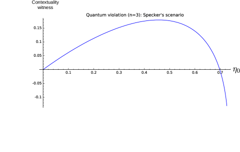
Figure 7.3: Specker’s scenario. In the middle figure, straight line denotes classical value.

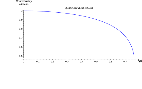
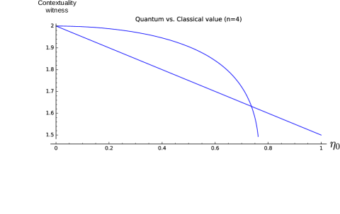
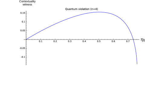
Figure 7.4: n=4 scenario. In the middle figure, straight line denotes classical value.

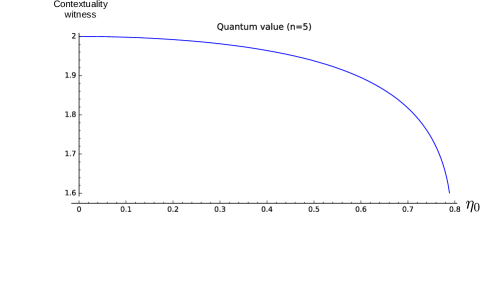
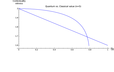
Figure 7.5: n=5 scenario. In the middle figure, straight line denotes classical value.

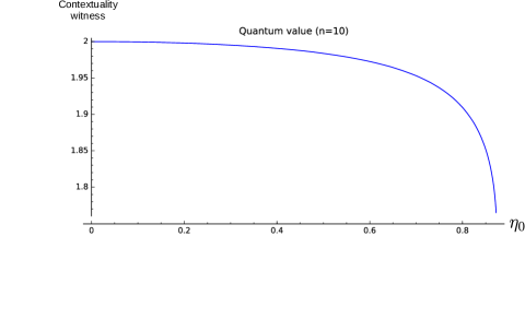
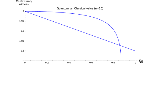
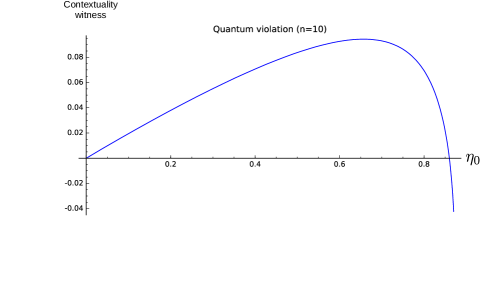
Figure 7.6: n=10 scenario. In the middle figure, straight line denotes classical value.

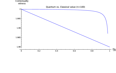
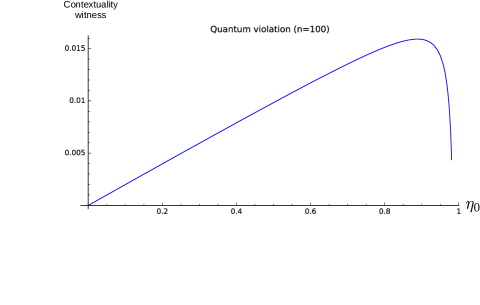
Figure 7.7: n=100 scenario. In the middle figure, straight line denotes classical value.

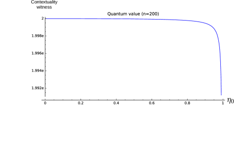
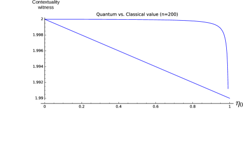
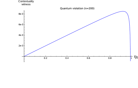
Figure 7.8: n=200 scenario. In the middle figure, straight line denotes classical value.

7.4 Chapter summary

As with the results of the previous chapter, the operational noncontextuality inequalities obtained in this chapter are also a significant improvement over previous proposals: they do not need the assumption of outcome-determinism, only the assumption of noncontextuality for preparations and measurements. Experimental testability, though, may still be a challenge for the two reasons we outlined in Chapter 6: firstly, the operational equivalences that we need to verify (in order for the assumption of noncontextuality to have nontrivial consequences) may only be approximately satisfied in a real experiment, and secondly, operational equivalence for preparation procedures is defined relative to all measurement procedures and that for measurement procedures relative to all preparation procedures, so an assumption of tomographic completeness is required in order that a finite set of preparations or measurements may be enough to verify the required operational equivalences. Testing the tomographic completeness of a finite set of experimental procedures when quantum theory is not assumed is another challenge. An approach to handling these issues—deviation from exact operational equivalence and testing the assumption of tomographic completeness—has been demonstrated in Ref. [63] (as also illustrated in Chapter 6). The same techniques can potentially be used to test the noncontextuality inequalities of this chapter in an experimentally robust manner.

In the previous chapter, we demonstrated how the so-called “state-independent” proofs of KS-contextuality, based on KS-uncolourability, can be turned into robust noncontextuality inequalities. In the present chapter we have turned so-called “state-dependent” proofs of KS-contextuality into robust noncontextuality inequalities. Hence, in line with previous work [63, 62], we have demonstrated that theory-independent tests of noncontextuality are possible, just like tests of local causality. The price we need to pay for such a theory-independent test, in the absence of a physical principle like no-faster-than-light-signalling coming to our rescue, is the requirement that the operational equivalence of experimental procedures must be verified explicitly rather than coming for “free” on account of spacelike separation (as in Bell experiments).

APPENDIX

Constraints from measurement noncontextuality – the n-cycle polytope

Once the operational equivalences of Eqs. (7.3.1) and (7.3.1) have been verified, the assumption of measurement noncontextuality places nontrivial bounds on the response functions in an ontological model, characterized by the $n$-cycle polytope (the so-called “no-disturbance” polytope of Ref. [61]). The $n$-cycle polytope, constrained only by normalization and positivity of probabilities, lives in $\mathbb{R}^{2n}$, has $2^{n}$ deterministic vertices and $2^{n-1}$ indeterministic vertices (see Ref. [61], in particular Theorem 2). Relabelling the outcome of each $M_{i}$ by $S_{i}\equiv(-1)^{X_{i}}$, where $X_{i}\in\{0,1\}$, the $2^{n}$ deterministic vertices of the n-cycle polytope are given by the vectors,

$$(\langle S_{1}\rangle,\dots,\langle S_{n}\rangle,\langle S_{1}\rangle\langle S_{2}\rangle,\dots,\langle S_{n}\rangle\langle S_{1}\rangle),$$ (7.37)

where $\langle S_{i}\rangle\in\{+1,-1\}$. The $2^{n-1}$ indeterministic vertices are given by the vectors

$$(0,\dots,0,\langle S_{1}S_{2}\rangle,\dots,\langle S_{n}S_{1}\rangle),$$ (7.38)

where $\langle S_{i}S_{i+1}\rangle\in\{+1,-1\}$ and the number of entries with $\langle S_{i}S_{i+1}\rangle=-1$ is odd. (Note that the addition $i+1$ is modulo $n$ so that for $i=n$, $n+1=1$.)

We denote the $2^{n}$ deterministic vertices by

$$\kappa_{\rm d}\in\big{\{}(\langle S_{1}\rangle,\dots,\langle S_{n}\rangle,\langle S_{1}\rangle\langle S_{2}\rangle,\dots,\langle S_{n}\rangle\langle S_{1}\rangle)|$$

$$\langle S_{i}\rangle\in\{-1,+1\}\forall i\in\{1,\dots,n\}\big{\}},$$ (7.39)

and the $2^{n-1}$ indeterministic vertices by

$$\kappa_{\rm in}\in\{(0,\dots,0,\langle S_{1}S_{2}\rangle,\dots,\langle S_{n}S_{1}\rangle)|\langle S_{i}S_{i+1}\rangle\in\{-1,+1\},$$

$$\text{odd number of }\langle S_{i}S_{i+1}\rangle=-1,i\in\{1,\dots,n\}\}.$$

Also, we let $\kappa$ denote any vertex (deterministic or indeterministic) of the $n$-cycle polytope.

For measurement $M_{i}$, $i\in\{1,\dots,n\}$, and a given ontic state $\lambda\in\Lambda$, we can define:

$$\zeta(M_{i},\lambda)\equiv\max_{S_{i}\in\{+1,-1\}}\xi(S_{i}|M_{i},\lambda).$$ (7.41)

Now:

$$\zeta(M_{i},\lambda) = \max_{S_{i}\in\{+1,-1\}}\sum_{\kappa}\xi(S_{i}|M_{i},\kappa)\mu(\kappa|\lambda)$$ (7.42)

$$\leq \sum_{\kappa}\max_{S_{i}\in\{+1,-1\}}\xi(S_{i}|M_{i},\kappa)\mu(\kappa|\lambda)$$ (7.43)

$$\equiv \sum_{\kappa}\zeta(M_{i},\kappa)\mu(\kappa|\lambda),$$ (7.44)

so that $\zeta(M_{i},\kappa)=\max_{S_{i}\in\{+1,-1\}}\xi(S_{i}|M_{i},\kappa)$.

We note that:

$$\zeta(M_{i},\kappa_{\rm d})=1,$$ (7.45)

$$\zeta(M_{i},\kappa_{\rm in})=\frac{1}{2},$$ (7.46)

for all deterministic and indeterministic vertices, respectively.

We then have:

$$\zeta(M_{i},\lambda)$$ (7.48)

$$\leq \frac{1}{2}\mu(\{\kappa_{\rm in}\}|\lambda)+\mu(\{\kappa_{\rm d}\}|\lambda)$$ (7.49)

$$= \frac{1}{2}(1-\mu(\{\kappa_{\rm d}\}|\lambda))+\mu(\{\kappa_{\rm d}\}|\lambda)$$ (7.50)

$$= \frac{1}{2}(1+\mu(\{\kappa_{\rm d}\}|\lambda)),$$ (7.51)

where $\{\kappa_{\rm in}\}$ denotes the set of all indeterministic vertices and $\{\kappa_{\rm d}\}$ denotes the set of all deterministic vertices.

We have used the fact that $\forall\kappa:\mu(\kappa|\lambda)\geq 0,$ $\sum_{\kappa}\mu(\kappa|\lambda)=\mu(\{\kappa_{\rm in}\}|\lambda)+\mu(\{\kappa_{\rm d}\}|\lambda)=1$. We can rewrite the last inequality on $\zeta(M_{i},\lambda)$ as:

$$\mu(\{\kappa_{\rm d}\}|\lambda)\geq\eta(M_{i},\lambda),$$ (7.52)

where $\eta(M_{i},\lambda)\equiv 2\zeta(M_{i},\lambda)-1$ and $i\in\{1,\dots,n\}$, so that $\mu(\{\kappa_{\rm d}\}|\lambda)\geq\max_{i}\eta(M_{i},\lambda)$. Further:

$$\max_{i\in\{1,\dots,n\}}\eta(M_{i},\lambda)\geq\frac{1}{n}\sum_{i=1}^{n}\eta(M_{i},\lambda),$$ (7.53)

which implies:

$$\mu(\{\kappa_{\rm d}\}|\lambda)\geq\frac{1}{n}\sum_{i=1}^{n}\eta(M_{i},\lambda).$$ (7.54)

Odd n-cycle

For odd $n$, the quantity of interest is

$$\xi({\rm anti}|M_{*},\lambda)\equiv\frac{1}{n}\sum_{i=1}^{n}\xi(S_{i}S_{j}=-1|M_{ij},\lambda),$$ (7.55)

where for each $i$, $j=i+1\mod n$, and, of course,

$$\xi(S_{i}S_{j}=-1|M_{ij},\lambda) \equiv \xi(S_{i}=1,S_{j}=-1|M_{ij},\lambda)$$

$$+ \xi(S_{i}=-1,S_{j}=1|M_{ij},\lambda).$$

It is easy to verify the following:

1. Every deterministic vertex $\kappa_{\rm d}$ is such that $\xi({\rm anti}|M_{*},\kappa_{\rm d})\leq\frac{n-1}{n}$.

2. The unique indeterministic vertex corresponding to perfect anticorrelation, denoted by $\kappa_{*}\in\{\kappa_{\rm in}\}$, satisfies $\xi({\rm anti}|M_{*},\kappa_{*})=1$, since $\langle S_{i}S_{j}\rangle=-1$ for all $i\in\{1,\dots,n\}$ and $j=i+1\mod n$.

3. The remaining indeterministic vertices in $\{\kappa_{\rm in}\}\backslash\kappa_{*}$ satisfy $\xi({\rm anti}|M_{*},\kappa_{\rm in})\leq\frac{n-2}{n}$.

Now,

$$\xi({\rm anti}|M_{*},\lambda)=\sum_{\kappa}\xi({\rm anti}|M_{*},\kappa)\mu(\kappa|\lambda),$$ (7.57)

therefore

$$\xi({\rm anti}|M_{*},\lambda)$$

$$\leq \mu(\kappa_{*}|\lambda)+\frac{n-1}{n}\mu(\{\kappa_{\rm d}\}|\lambda)+\frac{n-2}{n}\mu(\{\kappa_{\rm in}\}\backslash\kappa_{*}|\lambda),$$

where $\mu(\kappa_{*}|\lambda)+\mu(\{\kappa_{\rm d}\}|\lambda)+\mu(\{\kappa_{\rm in}\}\backslash\kappa_{*}|\lambda)=1$ for each $\lambda\in\Lambda$. Writing $\mu(\kappa_{*}|\lambda)=1-\mu(\{\kappa_{\rm d}\}|\lambda)-\mu(\{\kappa_{\rm in}\}\backslash\kappa_{*}|\lambda)$, we obtain

$$\xi({\rm anti}|M_{*},\lambda)\leq 1-\frac{1}{n}\mu(\kappa_{\rm d}|\lambda).$$ (7.59)

Using Eq. (7.54), we therefore have

$$\xi({\rm anti}|M_{*},\lambda)\leq 1-\frac{1}{n^{2}}\sum_{i=1}^{n}\eta(M_{i},\lambda).$$ (7.60)

Even n-cycle

For even $n$, the quantity of interest is

$$\xi({\rm chained}|M_{*},\lambda) \equiv \frac{1}{n}\sum_{i=1}^{n-1}\xi(S_{i}S_{j}=1|M_{ij},\lambda)$$ (7.61)

$$+ \frac{1}{n}\xi(S_{n}S_{1}=-1|M_{n1},\lambda),$$

where for each $i$, $j=i+1$, and, of course,

$$\xi(S_{i}S_{j}=1|M_{ij},\lambda) \equiv \xi(S_{i}=1,S_{j}=1|M_{ij},\lambda)$$

$$+ \xi(S_{i}=-1,S_{j}=-1|M_{ij},\lambda).$$

It is easy to verify the following:

1. Every deterministic vertex $\kappa_{\rm d}$ is such that $\xi({\rm chained}|M_{*},\kappa_{\rm d})\leq\frac{n-1}{n}$.

2. The unique indeterministic vertex corresponding to perfect chained correlation, denoted by $\kappa_{*}\in\{\kappa_{\rm in}\}$, satisfies $\xi({\rm chained}|M_{*},\kappa_{*})=1$, since $\langle S_{i}S_{j}\rangle=1$ for all $i\in\{1,\dots,n-1\},j=i+1$ and $\langle S_{n}S_{1}\rangle=-1$.

3. The remaining indeterministic vertices in $\{\kappa_{\rm in}\}\backslash\kappa_{*}$ satisfy $\xi({\rm chained}|M_{*},\kappa_{\rm in})\leq\frac{n-2}{n}$.

Now,

$$\xi({\rm chained}|M_{*},\lambda)=\sum_{\kappa}\xi({\rm chained}|M_{*},\kappa)\mu(\kappa|\lambda),$$ (7.63)

therefore

$$\xi({\rm chained}|M_{*},\lambda)$$

$$\leq \mu(\kappa_{*}|\lambda)+\frac{n-1}{n}\mu(\{\kappa_{\rm d}\}|\lambda)+\frac{n-2}{n}\mu(\{\kappa_{\rm in}\}\backslash\kappa_{*}|\lambda),$$

where $\mu(\kappa_{*}|\lambda)+\mu(\{\kappa_{\rm d}\}|\lambda)+\mu(\{\kappa_{\rm in}\}\backslash\kappa_{*}|\lambda)=1$ for each $\lambda\in\Lambda$. Writing $\mu(\kappa_{*}|\lambda)=1-\mu(\{\kappa_{\rm d}\}|\lambda)-\mu(\{\kappa_{\rm in}\}\backslash\kappa_{*}|\lambda)$, we obtain

$$\xi({\rm chained}|M_{*},\lambda)\leq 1-\frac{1}{n}\mu(\kappa_{\rm d}|\lambda).$$ (7.65)

Using Eq. (7.54), we therefore have

$$\xi({\rm chained}|M_{*},\lambda)\leq 1-\frac{1}{n^{2}}\sum_{i=1}^{n}\eta(M_{i},\lambda).$$ (7.66)

Based on Eqs. (7.60) and (7.66), we can now state a lemma—derived, as above, from the assumption of measurement noncontextuality—that will be useful in our proof of the noncontextuality inequalities:

Lemma 5.

For odd $n\geq 3$,

$$\xi({\rm anti}|M_{*},\lambda)\leq 1-\frac{1}{n^{2}}\sum_{i=1}^{n}\eta(M_{i},\lambda).$$ (7.67)

The same bound holds for $\xi({\rm anti}|M^{\prime}_{*},\lambda)$. Also, for even $n\geq 4$,

$$\xi({\rm chained}|M_{*},\lambda)\leq 1-\frac{1}{n^{2}}\sum_{i=1}^{n}\eta(M_{i},\lambda).$$ (7.68)

The same bound holds for $\xi({\rm chained}|M^{\prime}_{*},\lambda)$.

Remember, there are two $n$-cycle polytopes, one associated with joint measurements $\{M_{ij}\}$ and the other associated with joint measurements $\{M^{\prime}_{ij}\}$. Inequalities analogous to Eqs. (7.60) and (7.66), derived for the $\{M_{ij}\}$ polytope, also hold for the polytope associated with primed measurements $\{M^{\prime}_{ij}\}$. This is the content of Lemma 5.

Note that if, at a particular value of $\lambda$, all the measurements depend deterministically on $\lambda$, so that $\forall i,\eta(M_{i},\lambda)=1$, then we recover the bounds for an outcome-deterministic noncontextual ontological model, given by $\xi({\rm anti}|M_{*},\lambda)\leq\frac{n-1}{n}$ (similarly for $M^{\prime}_{*}$) and $\xi({\rm chained}|M_{*},\lambda)\leq\frac{n-1}{n}$ (similarly for $M^{\prime}_{*}$) for odd and even $n$, respectively. If, on the other extreme, at a particular value of $\lambda$, all the measurements are independent of $\lambda$, so that $\forall i,\eta(M_{i},\lambda)=0$, then the bounds become trivial, $\xi({\rm anti}|M_{*},\lambda)\leq 1$ and $\xi({\rm chained}|M_{*},\lambda)\leq 1$ (similarly for $M^{\prime}_{*}$): there is no obstacle to seeing perfect anticorrelation (for odd $n$) or perfect chained correlation (for even $n$) in a measurement noncontextual ontological model in this case.

It now remains to use the assumption of preparation noncontextuality to obtain the operational noncontextuality inequalities of Theorems 13 and 14.

Proof of Theorems 13 and 14

In this appendix we prove the inequalities in Theorem 14. The inequalities in Theorem 13 are a special case of these inequalities when $n=3$.

We define the operational predictability of measurement $M$, implemented following a preparation $P$, as

$$\eta(M,P)\equiv 2\max_{X\in\{0,1\}}p(X|M,P)-1.$$ (7.69)

Recall that the ontological predictability, defined earlier, is given by $\eta(M,\lambda)=2\max_{X\in\{0,1\}}\xi(X|M,P)-1$.

Lemma 6.

The ontological predictability of $M$ given $\lambda$, $\eta(M,\lambda)$, averaged over $\mu(\lambda|P)$, must be at least as great as the operational predictability of $M$ given $P$,

$$\sum_{\lambda\in\Lambda}\eta(M,\lambda)\mu(\lambda|P)\geq\eta(M,P).$$

Proof.

$$\eta(M,P)=2\max_{X\in\{0,1\}}p(X|M,P)-1$$

$$= 2\max_{X\in\{0,1\}}\sum_{\lambda\in\Lambda}\xi(X|M,\lambda)\mu(\lambda|P)-1$$

$$\leq 2\sum_{\lambda\in\Lambda}\max_{X\in\{0,1\}}\xi(X|M,\lambda)\mu(\lambda|P)-1$$

$$= \sum_{\lambda\in\Lambda}\eta(M,\lambda)\mu(\lambda|P).$$

∎

From the requirement that the ontological model reproduces the operational predictions, it follows that: for odd $n\geq 3$

$$p({\rm anti}|M_{*},P_{*})+p({\rm anti}|M^{\prime}_{*},P^{\perp}_{*})$$

$$=\sum_{\lambda\in\Lambda}\xi({\rm anti}|M_{*},\lambda)\mu(\lambda|P_{*})+\sum_{\lambda\in\Lambda}\xi({\rm anti}|M^{\prime}_{*},\lambda)\mu(\lambda|P^{\perp}_{*})$$

$$\leq 2-\frac{1}{n^{2}}\sum_{\lambda\in\Lambda}\sum_{i=1}^{n}\eta(M_{i},\lambda)\left(\mu(\lambda|P_{*})+\mu(\lambda|P^{\perp}_{*})\right),$$ (7.70)

where the last inequality is a consequence of Lemma 5. Similarly, for even $n\geq 4$

$$p({\rm chained}|M_{*},P_{*})+p({\rm chained}|M^{\prime}_{*},P^{\perp}_{*})$$

$$=\sum_{\lambda\in\Lambda}\xi({\rm chained}|M_{*},\lambda)\mu(\lambda|P_{*})+\sum_{\lambda\in\Lambda}\xi({\rm chained}|M^{\prime}_{*},\lambda)\mu(\lambda|P^{\perp}_{*})$$

$$\leq 2-\frac{1}{n^{2}}\sum_{\lambda\in\Lambda}\sum_{i=1}^{n}\eta(M_{i},\lambda)\left(\mu(\lambda|P_{*})+\mu(\lambda|P^{\perp}_{*})\right),$$ (7.71)

where we have again used Lemma 5.

We now make use of the assumption of preparation noncontextuality. Recalling the assumed operational equivalences among preparations (which have to be experimentally verified), Eq. (7.24), the definition of preparation noncontextuality, and how mixtures of preparation procedures are represented in an ontological model, we infer that

$$\forall i:\frac{1}{2}\mu(\lambda|P_{*})+\frac{1}{2}\mu(\lambda|P^{\perp}_{*})$$

$$=\frac{1}{2}\mu(\lambda|P_{i})+\frac{1}{2}\mu(\lambda|P^{\perp}_{i}).$$ (7.72)

It then follows that

$$p({\rm anti}|M_{*},P_{*})+p({\rm anti}|M^{\prime}_{*},P^{\perp}_{*})$$

$$\leq 2-\frac{1}{n^{2}}\sum_{\lambda\in\Lambda}\sum_{i=1}^{n}\eta(M_{i},\lambda)(\mu(\lambda|P_{i})+\mu(\lambda|P^{\perp}_{i}))$$

for odd $n\geq 3$ and

$$p({\rm chained}|M_{*},P_{*})+p({\rm chained}|M^{\prime}_{*},P^{\perp}_{*})$$

$$\leq 2-\frac{1}{n^{2}}\sum_{\lambda\in\Lambda}\sum_{i=1}^{n}\eta(M_{i},\lambda)(\mu(\lambda|P_{i})+\mu(\lambda|P^{\perp}_{i})),$$

for even $n\geq 4$.

Finally, making use of the bound derived in lemma 6, we obtain the operational inequality

$$p({\rm anti}|M_{*},P_{*})+p({\rm anti}|M^{\prime}_{*},P^{\perp}_{*})$$

$$\leq 2-\frac{1}{n^{2}}\sum_{i=1}^{n}\left(\eta(M_{i},P_{i})+\eta(M_{i},P^{\perp}_{i})\right)$$

$$=2\left(1-\frac{1}{n}\eta_{\rm ave}\right),$$ (7.75)

where

$$\eta_{\rm ave}\equiv\frac{1}{2n}\sum_{i=1}^{n}\left(\eta(M_{i},P_{i})+\eta(M_{i},P^{\perp}_{i})\right).$$ (7.76)

which completes the proof of the inequality in Eq. (7.25) for odd $n\geq 3$. For even $n\geq 4$

$$p({\rm chained}|M_{*},P_{*})+p({\rm chained}|M^{\prime}_{*},P^{\perp}_{*})$$

$$\leq 2-\frac{1}{n^{2}}\sum_{i=1}^{n}\left(\eta(M_{i},P_{i})+\eta(M_{i},P^{\perp}_{i})\right)$$

$$=2\left(1-\frac{1}{n}\eta_{\rm ave}\right),$$ (7.77)

which is the inequality in Eq.(7.26) for even $n\geq 4$.

Now, for the other four inequalities in Eqs. (7.28)-(14) and Eqs. (7.30)-(14):

$$p({\rm anti}|M_{*},P_{*})+p({\rm anti}|M_{*},P^{\perp}_{*})$$

$$=\sum_{\lambda\in\Lambda}\xi({\rm anti}|M_{*},\lambda)(\mu(\lambda|P_{*})+\mu(\lambda|P^{\perp}_{*}))$$

$$\leq\sum_{\lambda\in\Lambda}\left(1-\frac{1}{n^{2}}\sum_{i=1}^{n}\eta(M_{i},\lambda)\right)\left(\mu(\lambda|P_{*})+\mu(\lambda|P^{\perp}_{*})\right)$$

$$\leq 2-\frac{1}{n^{2}}\sum_{i=1}^{n}\left(\eta(M_{i},P_{i})+\eta(M_{i},P^{\perp}_{i})\right)$$

$$=2\left(1-\frac{1}{n}\eta_{\rm ave}\right),$$ (7.78)

which is the inequality of Eq.(7.28). Similarly, the inequality of Eq.(7.30) can be shown to hold. To obtain Eqs.(14) and (14), note that

$$\eta_{\rm ave}=\frac{1}{2n}\sum_{i=1}^{n}\left(\eta(M_{i},P_{i})+\eta(M_{i},P^{\perp}_{i})\right)$$

$$\leq \frac{1}{2n}\sum_{i=1}^{n}\left(\sum_{\lambda\in\Lambda}\eta(M_{i},\lambda)\mu(\lambda|P_{i})+\sum_{\lambda\in\Lambda}\eta(M_{i},\lambda)\mu(\lambda|P^{\perp}_{i})\right)$$

$$\text{(using lemma }\ref{lemma:predictability}\text{)},$$

$$= \frac{1}{2n}\sum_{i=1}^{n}\sum_{\lambda\in\Lambda}\eta(M_{i},\lambda)\left(\mu(\lambda|P_{i})+\mu(\lambda|P^{\perp}_{i})\right),$$

$$= \frac{1}{2n}\sum_{\lambda\in\Lambda}\sum_{i=1}^{n}\eta(M_{i},\lambda)\left(\mu(\lambda|P_{*})+\mu(\lambda|P^{\perp}_{*})\right)$$

(using preparation noncontextuality)

$$\leq \frac{1}{2n}\sum_{\lambda\in\Lambda}\sum_{i=1}^{n}\eta(M_{i},\lambda)\mu(\lambda|P_{*})+\frac{1}{2},$$

$$\text{(using the fact that }\sum_{i=1}^{n}\eta(M_{i},\lambda)\leq n\text{ in the second term)},$$

so that

$$\frac{1}{n^{2}}\sum_{\lambda\in\Lambda}\sum_{i=1}^{n}\eta(M_{i},\lambda)\mu(\lambda|P_{*})\geq\frac{1}{n}(2\eta_{\rm ave}-1)$$ (7.79)

and

$$p({\rm anti}|M_{*},P_{*}) = \sum_{\lambda\in\Lambda}\xi({\rm anti}|M_{*},\lambda)\mu(\lambda|P_{*})$$ (7.80)

$$\leq \sum_{\lambda\in\Lambda}\left(1-\frac{1}{n^{2}}\sum_{i=1}^{n}\eta(M_{i},\lambda)\right)\mu(\lambda|P_{*})$$

(using measurement noncontextuality, lemma 5)

$$\leq \frac{n-1}{n}+\frac{2}{n}(1-\eta_{\rm ave}),$$

which is Eq. (14). Eq. (14) can be obtained similarly.

Chapter 8 Future directions

In this thesis, I have reported progress towards making contextuality an experimentally testable notion of nonclassicality, based on work I have jointly carried out with various collaborators. In the first chapter, we introduced the framework of operational theories and ontological models within which discussions of contextuality are carried out in this thesis. In the second chapter, we showed how Specker’s scenario admits contextuality with respect to the LSW inequality. The third chapter examined the relationship between joint measurability and contextuality in quantum theory. The fourth chapter demonstrated how any joint measurability structure is realizable in quantum theory, opening up the possibility of contextuality in scenarios not envisaged by the Kochen-Specker theorem. In the fifth chapter, we argued why Fine’s theorem does not absolve one of the need to justify outcome determinism in ontological models of quantum theory. In chapter six we showed how to obtain robust noncontextuality inequalities directly inspired by the Kochen-Specker theorem in arbitrary operational theories. We also outlined a procedure for handling the problem of inexact operational equivalences in tests of noncontextuality, exemplified by the adoption of this procedure in the experiment of Ref. [63]. In the seventh chapter, we returned to Specker’s scenario and provided an analysis independent of quantum theory, unlike the analysis in the second chapter. We also generalized the insights from Specker’s scenario to arbitrary $n$-cycle scenarios and provided noncontextuality inequalities for these scenarios.

All this work opens up the opportunity to pursue a full development of contextuality into a comprehensive tool that can be used to detect the “nonclassicality” or “quantumness” of phenomena in a wide variety of physical scenarios. An important challenge is to build a quantitative bridge connecting our work to previous work in Kochen-Specker contextuality, in particular the graph-theoretic characterization of contextuality scenarios [25, 26], and bring this work within the ambit of the operational approach to contextuality due to Spekkens [6]. This would unify these approaches quantitatively and open the door to harnessing this nonclassicality for concrete information-theoretic tasks not relying on Bell tests. So far, Bell tests – experiments requiring (at least) two distant nonsignalling parties – are the gold standard for tests of nonclassicality. Work on contextuality along these lines could potentially yield ways of certifying nonclassicality that can be implemented within the same laboratory, covering a whole range of experimental scenarios that are not of the Bell type. Akin to Bell tests, the “no-go” conclusions drawn from these experiments would not rely on the validity of quantum theory. One also needs to extend the scope of the graph-theoretic framework to include contextuality scenarios that, in quantum theory, are only realizable with nonprojective observables [47]. The precise nature of the relation between Bell scenarios and tests of contextuality, beyond the folklore that considers Bell nonlocality a special case of contextuality, is worth exploring in view of recent results on contextuality à la Spekkens [71]. Indeed, following recent progress in understanding Bell experiments in terms of causal structure [78], I would also like to investigate whether, and to what extent, contextuality could be formulated in an appropriate causal framework that generalizes the framework adopted for Bell scenarios [79].

It would also be important to investigate contextuality as a resource in quantum information theory and study the robustness of this resource, perhaps in terms of channels that “break” it: with an appropriate definition of “contextuality breaking” channels in hand, one could expect to draw connections with the previously studied cases of channels that break entanglement, incompatibility, nonlocality, and nonclassicality[80]. Indeed, since noise is expected to destroy contextuality, part of the motivation here is to also study the robustness of the “magic for quantum computation” that contextuality (in the Kochen-Specker framework) supplies [4, 5]. The Spekkens’ framework for contextuality allows a robustness analysis of this sort and proving noise thresholds beyond which the “magic” is lost is a necessary exercise in order to understand the precise relationship between contextuality and practical quantum computation. Evidence of the role that (Kochen-Specker) contextuality plays in measurement based quantum computing [5] also needs to be subjected to such a robustness analysis in the Spekkens’ framework.

Finally, an interesting avenue is to investigate whether there’s a concrete connection between contextuality and other examples of quantum “weirdness”[81]. The motivation here is to ask whether contextuality is indeed the nonclassical feature of quantum theory that implies (or is implied by) all its other “weird” features, in particular features responsible for claimed quantum-over-classical advantages. If so, then we can claim to have found a characterization of nonclassicality that clearly separates quantum theory from attempts at its classical simulations, particularly in scenarios not of the Bell type. If not, then the challenge will be to identify what noncontextual part of quantum theory is still nonclassical, where this nonclassicality cannot be attributed to a restriction on how much any agent can know about the physical state of a system (that is, an “epistemic restriction”). We already know that a lot of the features of quantum theory can be simulated in classical theories imposing an epistemic restriction[82]. These theories, however, are local and noncontextual, so they cannot reproduce all of quantum theory: they are only “weakly nonclassical”.

In conclusion, let me again emphasize that the work presented in this thesis does not fall in the same category as much of the work in the existing literature on contextuality in the traditional Kochen-Specker paradigm (such as [25, 26]). In going beyond the Kochen-Specker theorem, this thesis contributes towards the project of developing a strictly operational understanding of contextuality.

Bibliography

- [1] S. Kochen and E. P. Specker, The Problem of Hidden Variables in Quantum Mechanics, J. Math. Mech. 17, 59 (1967). Available at Indiana University Mathematics Journal 17, 59 (1968), http://dx.doi.org/10.1512/iumj.1968.17.17004.
- [2] J. S. Bell, On the Einstein-Podolsky-Rosen Paradox, Physics 1, 195 (1964). Reprinted in Ref. [4], chap. 2.
- [3] J. S. Bell, On the problem of hidden variables in quantum mechanics, Rev. Mod. Phys. 38, 447 (1966); Reprinted in Ref. [4], chap. 1.
- [4] J. S. Bell, Speakable and unspeakable in quantum mechanics (Cambridge University Press, New York, 1987).
- [5] J. S. Bell, Epistemological Lett. 9 (1976) (Reproduced in Bell M, Gottfried K and Veltman M (ed) 2001 John S Bell on the Foundations of Quantum Mechanics (Singapore: World Scientific)).
- [6] N. Brunner, D. Cavalcanti, S. Pironio, V. Scarani, and S. Wehner, Bell nonlocality, Rev. Mod. Phys., 86, 2, 419–478 (2014). arXiv:1303.2849 [quant-ph].
- [7] D. A. Meyer, Finite Precision Measurement Nullifies the Kochen-Specker Theorem, Phys. Rev. Lett. 83, 3751 (1999), arXiv:quant-ph/9905080; A. Kent, Noncontextual Hidden Variables and Physical Measurements, Phys. Rev. Lett. 83, 3755 (1999), arXiv:quant-ph/9906006; R. Clifton and A. Kent, Simulating quantum mechanics by non-contextual hidden variables, Proc. R. Soc. Lond. A: 2000 456 2101-2114 (2000), arXiv:quant-ph/9908031; J. Barrett and A. Kent, Non-contextuality, finite precision measurement and the Kochen-Specker theorem, Stud. Hist. Philos. Mod. Phys. 35, 151 (2004), arXiv:quant-ph/0309017.
- [8] M. Howard, J. Wallman, V. Veitch, and J. Emerson, Contextuality supplies the ‘magic’ for quantum computation Nature 510, 351–355 (2014), arXiv:1401.4174 [quant-ph]; R. Raussendorf, Contextuality in measurement-based quantum computation, Phys. Rev. A 88, 022322 (2013), arXiv:0907.5449 [quant-ph].
- [9] R. W. Spekkens, Contextuality for preparations, transformations, and unsharp measurements, Phys. Rev. A 71, 052108 (2005), arXiv:quant-ph/0406166.
- [10] See Section 1 of P. Forrest, The Identity of Indiscernibles, The Stanford Encyclopedia of Philosophy (2012).
- [11] E. P. Specker, Die Logik Nicht Gleichzeitig Entscheidbarer Aussagen, Dialectica 14, 239-246 (1960); English translation: M. P. Seevinck, E. Specker: “The logic of non-simultaneously decidable propositions" (1960), arXiv:1103.4537 (2011).
- [12] Y.C. Liang, and R.W. Spekkens, and H.M. Wiseman, Specker’s parable of the overprotective seer: A road to contextuality, nonlocality and complementarity, Phys. Rep. 506, 1 (2011), arXiv:1010.1273 [quant-ph].
- [13] R. Kunjwal and S. Ghosh, Minimal state-dependent proof of measurement contextuality for a qubit, Phys. Rev. A 89, 042118 (2014), arXiv:1305.7009 [quant-ph].
- [14] R. Kunjwal, A note on the joint measurability of POVMs and its implications for contextuality, arXiv:1403.0470 (2014).
- [15] R. Kunjwal, C, Heunen, and T. Fritz, Quantum realization of arbitrary joint measurability structures, Phys. Rev. A 89, 052126 (2014), arXiv:1311.5948 [quant-ph].
- [16] A. Fine, Hidden Variables, Joint Probability, and the Bell Inequalities, Phys. Rev. Lett. 48, 291 (1982).
- [17] R. Kunjwal, Fine’s theorem, noncontextuality, and correlations in Specker’s scenario, Phys. Rev. A 91, 022108 (2015), arXiv:1410.7760 [quant-ph].
- [18] R. Kunjwal and R. W. Spekkens, From the Kochen-Specker Theorem to Noncontextuality Inequalities without Assuming Determinism, Phys. Rev. Lett. 115, 110403 (2015), arXiv:1506.04150 [quant-ph].
- [19] M. D. Mazurek, M. F. Pusey, R. Kunjwal, K. J. Resch, R. W. Spekkens, An experimental test of noncontextuality without unphysical idealizations, Nat. Commun. 7:11780 doi: 10.1038/ncomms11780 (2016), arXiv:1505.06244 [quant-ph].
- [20] A. Cabello, J. Estebaranz, and G. Garcia-Alcaine, Bell-Kochen-Specker theorem: A proof with 18 vectors, Physics Letters A 212, 183 (1996), arXiv:quant-ph/9706009.
- [21] A. A. Klyachko, M. A. Can, S. Binicioǧlu, and A. S. Shumovsky, Simple Test for Hidden Variables in Spin-1 Systems, Phys. Rev. Lett. 101, 020403 (2008), arXiv:0706.0126 [quant-ph].
- [22] R. Kunjwal, Noncontextuality without determinism and admissible (in)compatibility relations: revisiting Specker’s parable, Perimeter Quantum Foundations seminar, PIRSA:14010102 (2014), http://pirsa.org/14010102/.

Bibliography

- [1] N. Harrigan and R. W. Spekkens, Einstein, Incompleteness, and the Epistemic View of Quantum States, Found. Phys. 40, 125 (2010). arXiv version: arXiv:0706.2661 [quant-ph].
- [2] N. Brunner, D. Cavalcanti, S. Pironio, V. Scarani, and S. Wehner, Bell nonlocality, Rev. Mod. Phys., 86, 2, 419 - 478 (2014). arXiv version: arXiv:1303.2849 [quant-ph].
- [3] R. W. Spekkens, Nonclassicality as the failure of noncontextuality, PIRSA:15050081 (2015).
- [4] M. Howard, J. Wallman, V. Veitch, and J. Emerson, Contextuality supplies the ‘magic’ for quantum computation, Nature 510, 351-355 (2014). arXiv version: arXiv:1401.4174 [quant-ph].
- [5] R. Raussendorf, Contextuality in measurement-based quantum computation, Phys. Rev. A 88, 022322 (2013). arXiv version: arXiv:0907.5449 [quant-ph].
- [6] R. W. Spekkens, Contextuality for preparations, transformations, and unsharp measurements, Phys. Rev. A 71, 052108 (2005). arXiv version: arXiv:quant-ph/0406166.
- [7] L. Hardy, Quantum ontological excess baggage, Stud. Hist. Philos. Mod. Phys. 35, 267-276 (2004).
- [8] M. S. Leifer, Is the Quantum State Real? An Extended Review of -ontology Theorems, Quanta 2014; 3:67–155. arXiv version: arXiv:1409.1570 [quant-ph].
- [9] See, for example, Section 1 of P. Forrest, The Identity of Indiscernibles, The Stanford Encyclopedia of Philosophy (2012).
- [10] S. Kochen and E. P. Specker, The Problem of Hidden Variables in Quantum Mechanics, Indiana University Mathematics Journal, 17, 59 (1967).
- [11] J. Barrett and A. Kent, Non-contextuality, finite precision measurement and the Kochen-Specker theorem, Stud. Hist. Philos. Mod. Phys. 35, 151 (2004). arXiv version: arXiv:quant-ph/0309017.
- [12] A.M. Gleason, Measures on the Closed Subspaces of a Hilbert Space, Indiana Univ. Math. J. 6 No. 4, 885-893 (1957).
- [13] J. S. Bell, On the problem of hidden variables in quantum mechanics, Rev. Mod. Phys. 38, 447 (1966); Reprinted in Ref. [64], chap. 1.
- [14] A. Cabello, J. Estebaranz, and G. Garcia-Alcaine, Bell-Kochen-Specker theorem: A proof with 18 vectors, Physics Letters A 212, 183 (1996). arXiv version: arXiv:quant-ph/9706009.
- [15] M. S. Leifer and O. J. E. Maroney, Maximally Epistemic Interpretations of the Quantum State and Contextuality, Phys. Rev. Lett. 110, 120401 (2013). arXiv version: arXiv:1208.5132 [quant-ph].
- [16] A. Einstein, B. Podolsky, and N. Rosen, Can Quantum-Mechanical Description of Physical Reality Be Considered Complete?, Phys. Rev. 47, 777 (1935).
- [17] J. S. Bell, On the Einstein-Podolsky-Rosen Paradox, Physics 1, 195 (1964). Reprinted in Ref. [64], chap. 2.
- [18] J. F. Clauser, M. A. Horne, A. Shimony, and R. A. Holt, Proposed Experiment to Test Local Hidden-Variable Theories, Phys. Rev. Lett. 23, 880 (1969).
- [19] C.J. Wood and R.W. Spekkens, The lesson of causal discovery algorithms for quantum correlations: causal explanations of Bell-inequality violations require fine-tuning, New J. Phys. 17, 033002 (2015). arXiv version: arXiv:1208.4119 [quant-ph].
- [20] B. Hensen et al., Loophole-free Bell Inequality Violation Using Electron Spins Separated by 1.3 Kilometres, Nature 526, 682 (2015). arXiv version: arXiv:1508.05949 [quant-ph].
- [21] M. Giustina et al., Significant-Loophole-Free Test of Bell’s Theorem with Entangled Photons, Phys. Rev. Lett. 115, 250401 (2015). arXiv version: arXiv:1511.03190 [quant-ph].
- [22] L. K. Shalm et al., Strong Loophole-Free Test of Local Realism, Phys. Rev. Lett. 115, 250402 (2015). arXiv version: arXiv:1511.03189 [quant-ph].
- [23] J. S. Bell, The Theory of Local Beables, Epistemological Lett. 9 (1976) (Reproduced in Bell M, Gottfried K and Veltman M (ed) 2001 John S Bell on the Foundations of Quantum Mechanics (Singapore: World Scientific)). Available online at http://cds.cern.ch/record/980036/files/197508125.pdf.
- [24] R. Chaves and T. Fritz, Entropic approach to local realism and noncontextuality, Phys. Rev. A 85, 032113 (2012). arXiv version: arXiv:1201.3340 [quant-ph].
- [25] A. Cabello, S. Severini, and A. Winter, Graph-Theoretic Approach to Quantum Correlations, Phys. Rev. Lett. 112, 040401 (2014). arXiv version: arXiv:1401.7081 [quant-ph].
- [26] A. Acin, T. Fritz, A. Leverrier, and A. B. Sainz, A Combinatorial Approach to Nonlocality and Contextuality, Comm. Math. Phys. 334(2), 533-628 (2015). arXiv version: arXiv:1212.4084 [quant-ph].
- [27] D. A. Meyer, Finite Precision Measurement Nullifies the Kochen-Specker Theorem, Phys. Rev. Lett. 83, 3751 (1999), arXiv:quant-ph/9905080; A. Kent, Noncontextual Hidden Variables and Physical Measurements, Phys. Rev. Lett. 83, 3755 (1999), arXiv:quant-ph/9906006; R. Clifton and A. Kent, Simulating quantum mechanics by non-contextual hidden variables, Proc. R. Soc. Lond. A: 2000 456 2101-2114 (2000), arXiv:quant-ph/9908031; J. Barrett and A. Kent, Non-contextuality, finite precision measurement and the Kochen-Specker theorem, Stud. Hist. Philos. Mod. Phys. 35, 151 (2004), arXiv:quant-ph/0309017.
- [28] E. P. Specker, Die Logik Nicht Gleichzeitig Entscheidbarer Aussagen, Dialectica 14, 239-246 (1960); English translation: M. P. Seevinck, E. Specker: "The logic of non-simultaneously decidable propositions" (1960), arXiv:1103.4537 (2011).
- [29] Y.C. Liang, and R.W. Spekkens, and H.M. Wiseman, Specker’s parable of the overprotective seer: A road to contextuality, nonlocality and complementarity, Phys. Rep. 506, 1 (2011). arXiv version: arXiv:1010.1273 [quant-ph].
- [30] R. Kunjwal and S. Ghosh, Minimal state-dependent proof of measurement contextuality for a qubit, Phys. Rev. A 89, 042118 (2014). arXiv version: arXiv:1305.7009 [quant-ph].
- [31] R. Clifton, Getting contextual and nonlocal elements-of-reality the easy way, Am. J. Phys. 61, 443 (1993).
- [32] A. Peres, Two simple proofs of the Kochen-Specker theorem, J. Phys. A: Math. Gen. 24 L175 (1991).
- [33] N. D. Mermin, Hidden variables and the two theorems of John Bell, Rev. Mod. Phys., 65, 803 (1993).
- [34] A. Cabello and G. García-Alcaine, Bell-Kochen-Specker theorem for any finite dimension , J. Phys. A 29, 1025 (1996).
- [35] A. A. Klyachko, M. A. Can, S. Binicioǧlu, and A. S. Shumovsky, Simple Test for Hidden Variables in Spin-1 Systems, Phys. Rev. Lett. 101, 020403 (2008). arXiv version: arXiv:0706.0126 [quant-ph].
- [36] P. Kurzyński, R. Ramanathan, and D. Kaszlikowski, Entropic Test of Quantum Contextuality, Phys. Rev. Lett. 109, 020404 (2012). arXiv version: arXiv:1201.2865 [quant-ph].
- [37] S. Yu, and C. H. Oh, State-Independent Proof of Kochen-Specker Theorem with 13 Rays, Phys. Rev. Lett. 108, 030402 (2012). arXiv version: arXiv:1109.4396 [quant-ph].
- [38] A. Cabello, State-independent quantum contextuality and maximum nonlocality, arXiv:1112.5149 [quant-ph].
- [39] A. Cabello, Kochen-Specker Theorem for a Single Qubit using Positive Operator-Valued Measures, Phys. Rev. Lett. 90, 190401 (2003). arXiv version: arXiv:quant-ph/0210082.
- [40] P. Busch, Quantum States and Generalized Observables: A Simple Proof of Gleason’s Theorem, Phys. Rev. Lett. 91, 120403 (2003). arXiv version: arXiv:quant-ph/9909073.
- [41] C. M. Caves, C. A. Fuchs, K. K. Manne, and J. M. Renes, Gleason-Type Derivations of the Quantum Probability Rule for Generalized Measurements, Found. Phys. 34, 193 (2004).
- [42] R. W. Spekkens, The Status of Determinism in Proofs of the Impossibility of a Noncontextual Model of Quantum Theory, Found. Phys. 44, 11, 1125 (2014). arXiv version: arXiv:1312.3667 [quant-ph].
- [43] S. Yu, N. L. Liu, L. Li, and C. H. Oh, Joint measurement of two unsharp observables of a qubit, Phys. Rev. A 81, 062116 (2010). arXiv version: arXiv:0805.1538 [quant-ph].
- [44] T. Heinosaari, D. Reitzner, and P. Stano, Notes on Joint Measurability of Quantum Observables, Found. Phys. 38, 1133 (2008). arXiv version: arXiv:0811.0783 [quant-ph].
- [45] S. Yu, C. H. Oh, Quantum contextuality and joint measurement of three observables of a qubit, arXiv:1312.6470v1 [quant-ph].
- [46] R. Kunjwal, A note on the joint measurability of POVMs and its implications for contextuality, arXiv:1403.0470 (2014).
- [47] R. Kunjwal, C, Heunen, and T. Fritz, Quantum realization of arbitrary joint measurability structures, Phys. Rev. A 89, 052126 (2014). arXiv version: arXiv:1311.5948 [quant-ph].
- [48] C. Heunen, T. Fritz, and M. L. Reyes,Quantum theory realizes all joint measurability graphs, Phys. Rev. A 89, 032121 (2014). arXiv version: arXiv:1310.3698 [quant-ph].
- [49] K. Kraus, States, Effects, and Operations, Springer, 1983.
- [50] P. Stano, D. Reitzner, and T. Heinosaari, Coexistence of qubit effects, Phys. Rev. A 78, 012315 (2008). arXiv version: arXiv:0802.4248 [quant-ph].
- [51] P. Busch and H. J. Schmidt, ,Quantum Information Processing 9, 2, 143-169 (2010). arXiv version: arXiv:0802.4167 [quant-ph].
- [52] E. Andersson, S. M. Barnett, and A. Aspect, Joint measurements of spin, operational locality, and uncertainty, Phys. Rev. A 72, 042104 (2005). arXiv version: arXiv:quant-ph/0509152.
- [53] M. M. Wolf, D. Perez-Garcia, and C. Fernandez, Measurements Incompatible in Quantum Theory Cannot Be Measured Jointly in Any Other No-Signaling Theory, Phys. Rev. Lett. 103, 230402 (2009). arXiv version: arXiv:0905.2998 [quant-ph].
- [54] S. Abramsky and A. Brandenburger, The sheaf-theoretic structure of non-locality and contextuality, New J. Phys. 13, 113036 (2011). arXiv version: arXiv:1102.0264 [quant-ph].
- [55] P. Lounesto, Clifford Algebras and Spinors, London Mathematical Society Lecture Note Series (Book 286).
- [56] A. Fine, Hidden Variables, Joint Probability, and the Bell Inequalities, Phys. Rev. Lett. 48, 291 (1982).
- [57] A. Fine, Joint distributions, quantum correlations, and commuting observables, J. Math. Phys. 23, 1306 (1982).
- [58] R. Kunjwal, Fine’s theorem, noncontextuality, and correlations in Specker’s scenario, Phys. Rev. A 91, 022108 (2015). arXiv version: arXiv:1410.7760 [quant-ph].
- [59] H. M. Wiseman, The Two Bell’s theorems of John Bell, J. Phys. A: Math. Theor. 47 424001 (2014). arXiv version: arXiv:1402.0351 [quant-ph].
- [60] J. Barrett, L. Hardy, A. Kent, No Signaling and Quantum Key Distribution, Phys. Rev. Lett. 95, 010503 (2005). arXiv version: arXiv:quant-ph/0405101.
- [61] M. Araújo, M. T. Quintino, C. Budroni, M. T. Cunha, and A. Cabello, All noncontextuality inequalities for the n-cycle scenario, Phys. Rev. A 88, 022118 (2013). arXiv version: arXiv:1206.3212 [quant-ph].
- [62] R. Kunjwal and R. W. Spekkens, From the Kochen-Specker Theorem to Noncontextuality Inequalities without Assuming Determinism, Phys. Rev. Lett. 115, 110403 (2015). arXiv version: arXiv:1506.04150 [quant-ph].
- [63] M. D. Mazurek, M. F. Pusey, R. Kunjwal, K. J. Resch, R. W. Spekkens, An experimental test of noncontextuality without unphysical idealizations, Nat. Commun. 7:11780 doi: 10.1038/ncomms11780 (2016). arXiv version: arXiv:1505.06244 [quant-ph].
- [64] J. S. Bell, Speakable and unspeakable in quantum mechanics (Cambridge University Press, New York, 1987).
- [65] T. Norsen, Are there really two different Bell’s theorems, arXiv:1503.05017 [quant-ph].
- [66] Indeed, in Ref. [69], David Mermin is quoted as having said: “the whole notion of an experimental test of KS misses the point,” a view that was held by many researchers at the time.
- [67] L. Hardy, Quantum theory from five reasonable axioms, arXiv:quant-ph/0101012 (2001).
- [68] J. Barrett, Information processing in generalized probabilistic theories, Phys. Rev. A 75, 032304 (2007). arXiv version: arXiv:quant-ph/0508211.
- [69] A. Cabello and G. Garcia-Alcaine, Proposed Experimental Tests of the Bell-Kochen-Specker Theorem, Phys. Rev. Lett. 80, 1797 (1998). arXiv version: arXiv:quant-ph/9709047.
- [70] A. Cabello, Experimentally testable state-independent quantum contextuality, Phys. Rev. Lett. 101, 210401 (2008). arXiv version: arXiv:0808.2456 [quant-ph].
- [71] M. F. Pusey, The robust noncontextuality inequalities in the simplest scenario, arXiv:1506.04178 [quant-ph].
- [72] X. Zhan, J. Li, H. Qin, Z. Bian, Y. Zhang, P. Xue, Violation of a generalized non-contextuality inequality with single photons, arXiv:1505.06825 [quant-ph].
- [73] S. Braunstein and C. M. Caves, Wringing out better Bell inequalities, Ann. Phys. 202, 22 (1990).
- [74] SageMathCloud is available at https://cloud.sagemath.com
- [75] R. W. Spekkens, Negativity and Contextuality are Equivalent Notions of Nonclassicality, Phys. Rev. Lett. 101, 020401 (2008). arXiv version: arXiv:0710.5549 [quant-ph].
- [76] M. Krystek and M. Anton, A weighted total least-squares algorithm for fitting a straight line, Meas. Sci. Technol., 18, 3438 (2007).
- [77] W. H. Press, S. A. Teukolsky, W. T. Vetterling, and B. P. Flannery, Numerical Recipes: The Art of Scientific Computing, 3rd ed. (Cambridge University Press, New York, 2007).
- [78] J. Henson, R. Lal, M. F. Pusey, Theory-independent limits on correlations from generalised Bayesian networks, New J. Phys. 16, 113043 (2014). arXiv version: arXiv:1405.2572 [quant-ph].
- [79] R. W. Spekkens, Why I Am Not a Psi-ontologist, PIRSA:12050021.
- [80] M. Horodecki, P. W. Shor, and M. B. Ruskai, Entanglement breaking channels, Reviews in Mathematical Physics, 15(06), 629-641 (2003), arXiv:quant-ph/0302031; T. Heinosaari, J. Kiukas, D. Reitzner, J. Schultz, Incompatibility breaking quantum channels, J. Phys. A: Math. Theor. 48 (2015) 435301, arXiv:1504.05768 [quant-ph]; T. Heinosaari, J. Kiukas, and J. Schultz, Breaking Gaussian incompatibility on continuous variable quantum systems, J. Math. Phys. 56, 082202 (2015), arXiv:1505.00833 [quant-ph]; R. Pal and S. Ghosh, Non-locality breaking qubit channels, arXiv:1306.3151 [quant-ph]; J. S. Ivan, K. K. Sabapathy, and R. Simon, Nonclassicality breaking is the same as entanglement breaking for bosonic Gaussian channels, Phys. Rev. A 88, 032302 (2013), arXiv:1306.5536 [quant-ph].
- [81] R. W. Spekkens, Negativity and Contextuality are Equivalent Notions of Nonclassicality, Phys. Rev. Lett. 101, 020401 (2008), arXiv:0710.5549 [quant-ph]; M. F. Pusey, Anomalous Weak Values Are Proofs of Contextuality, Phys. Rev. Lett. 113, 200401 (2014), arXiv version: arXiv:1409.1535 [quant-ph].
- [82] R. W. Spekkens, Quasi-quantization: classical statistical theories with an epistemic restriction, arXiv:1409.5041 [quant-ph] (2014).