Emergence of Fresnel diffraction zones in gravitational lensing by a cosmic string

Abstract

The possibility to detect cosmic strings – topological defects of early Universe, by means of wave effects in gravitational lensing is discussed. To find the optimal observation conditions, we define the hyperbolic-shaped Fresnel observation zones associated with the diffraction maxima and analyse the frequency patterns of wave amplification corresponding to different alignments. In particular, we show that diffraction of gravitational waves by the string may lead to significant amplification at cosmological distances. The wave properties we found are quite different from what one would expect, for instance, from light scattered off a thin wire or slit, since a cosmic string, as a topological defect, gives no shadow at all.

I Introduction

The first direct detection of gravitational waves by the Laser Interferometer Gravitational-Wave Observatory (LIGO) LIGO16-1 opened up a new way to observe the Universe. Along with gravitational wave detection, it was the first direct observation of binary black holes. With this success, there are many hopes that other previously invisible cosmological objects, which emit or scatter gravitational waves, will be observed in the near future.

In this paper we discuss the possibility to detect cosmic strings – topological defects that may have been formed in the early Universe kibble76 ; vilenkin-shellard94 – by means of wave effects in the gravitational lensing taking into account the interference and diffraction. We emphasize the difference of wave diffraction on a topological defect from that on a compact object. For the wave effects to be detectable in a compact-mass gravitational lens, the wavelength $\lambda$ should be comparable or larger than the Schwarzschild radius $R_{\rm s}$ of the lens deguchi86 . In this case, the Fresnel number, which is the key parameter for the diffraction, is given by $R_{\rm s}/\lambda$, and the diffraction scales like $O(\lambda/R_{\rm s})$. This scaling cannot be applied to a string, a non-compact object with conical topology. It has been shown recently for the plane-wave diffraction by string pla-string16 that the Fresnel number is determined by the ratio $r\Delta^{2}/\lambda$, where $r$ is the distance from the string to the observer and $\Delta$ is a constant related to the deficit angle of conical space, which is proportional to the linear mass of the string vilenkin81 ; vilenkin84 ; gott85 . For the typical $\Delta\sim 10^{-7}$, low Fresnel numbers can be achieved at cosmological distances from the string, $r\sim 10^{14\,}\lambda$. As a result, the diffraction effects can be of the same order as the geometrical optics giving an additional amplification at the observation point pla-string16 . This is a direct consequence of the conical topology, for which the metric is locally flat, but globally it forces the parallel geodesics to cross (when they pass on opposite sides of the string) at a large distance. On the other hand, the deflection angle, equal to $\Delta$, is independent of the impact parameter vilenkin81 ; vilenkin84 . Hence, the characteristic fringe width in the interference pattern $\sim\lambda/(2\Delta)$ does not vary with distance. This is another feature distinct from the compact-object lens, for which the interference fringe scales with distance as $\sim\lambda\sqrt{r/R_{s}}$ nakamura98 .

The objective of this paper is twofold. First, we study the question of how the Fresnel diffraction zones emerge under wave propagation in conical spacetime created by a straight cosmic string . The diffraction pattern we have obtained is quite different from what one would expect from light scattered off a thin wire or slit sommerfeld54 ; born-wolf-03 , since the cosmic string, as a topological defect, gives no shadow. After an appropriately chosen coordinate transformation, we convert the problem of a single-source wave in conical space to a more tractable form with a locally Minkowskian line element and a limitation on the angular range. As a result, we obtain the interference and diffraction pattern analytically as a superposition of wave fields from two image sources illuminating two virtual half-plane screens.

Second, we take into account the curvature of the incident wavefront by considering the wave source at a finite distance from the string. This is a more general case with respect to our previous study pla-string16 . By applying the uniform asymptotic theory of diffraction boersma68 ; borovikov , we obtain analytical solutions for the wave field in the whole space including the lines of singularities at the boundaries of the double-imaging region. Away from the boundaries, the wave field is interpreted in the framework of Keller’s geometrical theory of diffraction keller62 , which has demonstrated to be quite efficient in studying diffraction on a topological defect pla-string16 . Our results allow to predict with high accuracy the location of the diffraction maxima both in coordinate space and in energy spectrum, along with the nodal and antinodal lines of geometrical-optics interference. We found it convenient to associate the diffraction maxima with what we call the “Fresnel observation zones”, that help to localize the regions where the amplification due to the string is the highest and easier to observe. The boundaries between the zones are determined by hyperbolas in an equivalent Minkowskian space. In the limit of an infinitely distant source (incident plane wave), the hyperbolas convert to parabolas, all with a common focus at the string.

II Wave equation in conical spacetime

We start with a spacetime metric for a static cylindrically symmetric cosmic string vilenkin81 ; gott85

$$\mathrm{d}s^{2}=-\mathrm{d}t^{2}+\mathrm{d}r^{2}+(1-4G\mu)^{2}r^{2}\mathrm{d}\varphi^{2}+\mathrm{d}z^{2},$$ (1)

where $G$ is the gravitational constant, $\mu$ is the linear mass density of the string lying along the $z$-axis, ($t,r,\varphi,z$) are cylindrical coordinates, and the system of units in which the speed of light $c=1$ is assumed. With a new angular coordinate $\theta=(1-4G\mu)\varphi$, the metric (1) takes a locally Minkowskian form

$$\mathrm{d}s^{2}=-\mathrm{d}t^{2}+\mathrm{d}r^{2}+r^{2}\mathrm{d}\theta^{2}+\mathrm{d}z^{2},$$ (2)

having, however, a limitation on the angular range. It is assumed here, that a wedge of angular size $8\pi G\mu$ is taken out and the two faces of the wedge are identified vilenkin81 ; vilenkin-shellard94 . By introducing the deficit angle $2\Delta$ with

$$\Delta=4\pi G\mu,$$ (3)

the angular coordinate $\theta$ spans the range $2\pi-2\Delta$.

We consider the question of finding a solution of the wave equation in background (1) corresponding to a time harmonic source, situated at a finite distance from the string. For the sake of simplicity, in order to keep the problem two-dimensional, we consider a line source parallel to the string. Our aim is to see how a wave emitted by a line source is diffracted in conical spacetime. The wave equation in background (1) for the scalar field $U(r,\varphi)$ is (see, e.g., pla-string16 ; linet86 ; suyama06 )

$$\left(\frac{\partial^{2}}{\partial r^{2}}+\frac{1}{r}\frac{\partial}{\partial r}+\frac{1}{\beta^{2}r^{2}}\frac{\partial^{2}}{\partial\varphi^{2}}+\omega^{2}\right)U=0,$$ (4)

where we denoted $\beta\equiv 1-\Delta/\pi$. We assume that Eq. (4) is valid for electromagnetic waves, as well as for gravitational waves (in an appropriately chosen gauge) when the effect of gravitational lensing on polarization is negligible and both types of waves can be described by a scalar field misner . Consider a line source $E$ located at $\mathbf{r_{0}}=(r_{0},\pi)$ and emitting a cylindrical wave described by

$$U=A\,H_{0}^{(1)}(k|\mathbf{r}-\mathbf{r_{0}}|),$$ (5)

where $A$ is a normalization constant and $H_{0}^{(1)}$ is the Hankel function of the first kind which satisfies the Helmholtz equation (4) and corresponds to an outward-propagating solution born-wolf-03 . It is advantageous to perform the angular transformation $\theta=\beta\varphi$ and to work in the Minkowskian geometry (2) with a wedge removed rather than in the metric (1), as done in Ref. pla-string16 for an infinitely distant source. To conveniently perform the transformation, we put the origin at the string location $S$ and join the point $S$ with the emitting source $E$ by a radial line [see Fig. 1(a)]. Then we assign the values $\varphi^{-}=-\pi$ to the left and $\varphi^{+}=\pi$ to the right of the line $SE$ that will be the cut line. Assuming that the emitting wave is symmetric (isotropic), we obtain a zero derivative $\partial_{\varphi}U=0$ at the cut. After the angular transformation, the line $SE$ converts to the wedge $SE^{-}$, $SE^{+}$, given by the angles $\pm(\pi-\Delta)$ [see Fig. 1(b)]. The two faces of the wedge should be identified since they represent the same plane in the spacetime (1). Thus, the propagation of a wave in conical spacetime can be represented as the propagation of two waves in flat geometry with a wedge removed. In our consideration, each emitting source lies on the corresponding face of the wedge. Our next step is to show that the problem posed in this section can be effectively treated in the framework of the canonical problem of diffraction on a perfectly conducting half-plane screen pla-string16 .

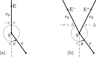
Figure 1: Geometry of conical space at the $z=0$ plane for two equivalent backgrounds with point $S$ indicating the location of the string: (a) polar coordinates $(r,\varphi)$ with a source $E$; (b) Minkowskian coordinates $(r,\theta)$ with deficit angle $2\Delta$ and two image sources $E^{-}$, $E^{+}$.

III Uniform asymptotic theory of diffraction on a half plane

Let us consider a half-plane screen defined in polar coordinates $(r,\alpha)$ by: $\alpha=0$ (upper surface) and $\alpha=2\pi$ (lower surface). According to our geometry, the source is located on the upper surface of the screen at a distance $r_{0}$ from the edge, i.e., at $(r_{0},0)$ (see Fig. 2).

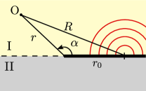
Figure 2: Cylindrical wave emitted from a source on the upper surface of a half-plane screen (thick line). The space is split into two regions: illuminated (I), shadow (II).

The emission field is a cylindrical wave that can be defined by born-wolf-03

$$U_{i}=\sqrt{\frac{\pi}{2}}\mathrm{e}^{\mathrm{i}\pi/4}\,H_{0}^{(1)}(kR)\approx\frac{\mathrm{e}^{\mathrm{i}kR}}{\sqrt{kR}},$$ (6)

with $R=\sqrt{r^{2}+r_{0}^{2}-2rr_{0}\cos\alpha}$ and the subscript “i” means “incident” field. The solution for the field in the whole space can be expressed as an integral macdonald ; clemmow50 ; bowman69 ; born-wolf-03

$$U=\displaystyle{\sqrt{\frac{2}{\pi}}\,e^{-\mathrm{i}\pi/4}\,e^{\mathrm{i}kR}\int_{-w}^{\infty}\frac{\mathrm{e}^{\mathrm{i}\mu^{2}}\mathrm{d}\mu}{\sqrt{\mu^{2}+2kR}}},$$ (7)

where $w=\sigma\sqrt{k(r+r_{0}-R})$, with $\sigma\equiv\mathrm{sgn}\left[\cos\left(\alpha/2\right)\right]$, a sign function giving $+1$ in the illuminated region and $-1$ in the shadow (see Fig. 2). Instead of working with the solution in the integral representation (7), we apply the uniform asymptotic theory boersma68 ; borovikov , which has proved to be quite accurate in finding solutions for the wave field under diffraction. We seek the solution in the form

$$U=U_{i}\,\mathcal{F}(w)+\mathcal{R},$$ (8)

where the first term is the penumbra field with the Fresnel integral defined by

$$\mathcal{F}(u)=\frac{1}{\sqrt{\pi\mathrm{i}}}\int_{-\infty}^{u}\mathrm{e}^{\mathrm{i}\mu^{2}}\mathrm{d}\mu$$ (9)

and $\mathcal{R}$ offsets the residual arising from substituting the penumbra term in the wave equation. In both Eqs. (7) and (8), the Neumann boundary condition for the field is assumed on the screen. The residual $\mathcal{R}$ has a form of the ray expansion

$$\mathcal{R}=e^{\mathrm{i}k(r+r_{0})}\sum_{n=1}^{\infty}k^{-n}C_{n},$$ (10)

in which the slowly varying coefficients $C_{n}$ can be determined by the method of asymptotic matching borovikov which consists in comparing the uniform asymptotics (8) with the nonuniform asymptotics of the rigorous solution and expanding all the terms with respect to inverse powers of $k$. The nonuniform expansion can be written as

$$U\approx U_{i}\,\mathcal{H}(w)+U_{i}^{0}\,D\,\frac{\mathrm{e}^{\mathrm{i}kr}}{\sqrt{kr}}.$$ (11)

Here, the first term is the geometrical-optics contribution of the incident wave. It is multiplied by the Heaviside step function $\mathcal{H}(w)$ that guarantees that this wave only contributes to the illuminated region. The second term is the leading order term $\sim O(k^{-1})$ of the diffracted field. It describes a cylindrical wave emanating from the edge (see, e.g., Ref. born-wolf-03 ). Its amplitude is given by the product of the incident wave evaluated at the edge, $U_{i}^{0}\equiv\mathrm{e}^{\mathrm{i}kr_{0}}/\sqrt{kr_{0}}$, and the diffraction coefficient keller62

$$D=-\frac{\mathrm{e}^{\mathrm{i}\pi/4}}{2\sqrt{2\pi}}\frac{1}{\cos(\alpha/2)}.$$ (12)

Note that the expansion (11), valid at $|w|\gg 1$, is nonuniform due to a singularity at $w=0$, that is, in the neighbourhood of the light-shadow boundary. It should also be remarked that the diffraction coefficient $D$ is determined by the geometry of the obstacle (a half plane in our case) but is independent of the type of incident wave keller62 ; kouyoumijan74 .

To do the asymptotic matching, the Fresnel integral (9) is replaced with its asymptotics at large arguments sommerfeld54

$$\mathcal{F}(w)\approx\mathcal{H}(w)-\frac{\mathrm{e}^{\mathrm{i}\pi/4}}{2\sqrt{\pi}}\,\frac{\mathrm{e}^{\mathrm{i}w^{2}}}{w}\equiv\mathcal{H}(w)-\mathcal{\tilde{F}}(w).$$ (13)

By comparing Eqs. (8) and (11) up to the order $O(k^{-1})$, we see that only $C_{1}$ is relevant in the expansion (10) and for the residual $\mathcal{R}$ we obtain

$$\mathcal{R}\approx U_{i}\,\mathcal{\tilde{F}}+U_{i}^{0}\,D\,\frac{\mathrm{e}^{\mathrm{i}kr}}{\sqrt{kr}}.$$ (14)

Substituting in Eq. (8), one can write the final solution

$$U\approx U_{i}\,(\mathcal{F}+\mathcal{\tilde{F}})+U_{i}^{0}\,D\,\frac{\mathrm{e}^{\mathrm{i}kr}}{\sqrt{kr}}.$$ (15)

Written in this form, the solution (15) corresponds to the uniform asymptotic theory introduced in Ref. boersma68 . It is called uniform since the poles in the diffraction coefficient $D$ are cancelled out by the poles in the term $\mathcal{\tilde{F}}$, giving a regular solution in the whole space including the light-shadow boundary. It would be convenient to combine both singular terms in one by defining a new diffraction coefficient

$$\tilde{D}=-\frac{\mathrm{e}^{\mathrm{i}\pi/4}}{2\sqrt{2\pi}}\left[\frac{1}{\cos(\alpha/2)}-\sigma\sqrt{\frac{2rr_{0}}{R(r+r_{0}-R)}}\right],$$ (16)

and the uniform solution finally becomes

$$U\approx U_{i}\,\mathcal{F}(w)+U_{i}^{0}\,\tilde{D}\,\frac{\mathrm{e}^{\mathrm{i}kr}}{\sqrt{kr}}.$$ (17)

Note that Eq. (17) is valid at any distances from the light-shadow boundary, near and away from the edge, i.e. everywhere except for the neighbourhood of the source, since $kR\gg 1$ is assumed. Far from the light-shadow boundary, both asymptotics, the nonuniform (11) and uniform one (17), coincide. We also observe that the edge wave has a phase shift of $-3\pi/4$ in the illuminated region and $+\pi/4$ in the shadow with respect to the incident field. Crossing the shadow line introduces a phase change of $\pi$, which is manifested in the sign change of the diffraction coefficients $D$ and $\tilde{D}$ (See the original work by Fresnel fresnel1821 ; crew1900 who pointed out that the diffracted waves in the shadow and illuminated regions are in complete phase opposition).

IV Diffraction of a cylindrical wave by a cosmic string

As explained in Sect. II, after an angular transformation, the spacetime (1) can be represented in the flat Minkowskian geometry (2) with a wedge of $2\Delta$ removed [Fig. 1(b)]. Accordingly, the wave source $E$ is doubled into images $E^{-}$, $E^{+}$ which are located on the faces of the wedge. Each image source emits a cylindrical wave that will be diffracted by the corresponding half plane. Therefore, the wave diffraction by a string can be thought of as the diffraction by two half planes forming an angle of $2\Delta$ pla-string16 .

We now construct the wave field by making use of the results described in the previous section for the case of a single half plane. We use the angular substitution $\alpha=\pi-\Delta\mp\theta$ for each half plane in order to work with the flat coordinates $(r,\theta)$. The emission field for each source is described by a cylindrical wave given by

$$U_{i}^{\pm}\approx\frac{\mathrm{e}^{\mathrm{i}ks^{\pm}}}{\sqrt{ks^{\pm}}},$$ (18)

where $s^{\pm}=\sqrt{r^{2}+r_{0}^{2}+2rr_{0}\cos(\Delta\pm\theta)}$. From Eq. (17), the uniform asymptotic solution for the field at the observation point $(r,\theta)$ is found in the form

$$U=U_{i}^{-}\mathcal{F}(w^{-})+U_{i}^{+}\mathcal{F}(w^{+})+U_{i}^{0}\left(\tilde{D}^{-}+\tilde{D}^{+}\right)\frac{\mathrm{e}^{\mathrm{i}kr}}{\sqrt{kr}},$$ (19)

with the modified diffraction coefficients $\tilde{D}^{\pm}$ defined as

$$\tilde{D}^{\pm}=-\frac{\mathrm{e}^{\mathrm{i}\pi/4}}{2\sqrt{2\pi}}\left[\frac{1}{\sin{[\frac{1}{2}(\Delta\pm\theta})]}-\sigma^{\pm}\sqrt{\frac{2rr_{0}}{s^{\pm}(r+r_{0}-s^{\pm})}}\right],$$ (20)

and the notations $w^{\pm}=\sigma^{\pm}\sqrt{k(r+r_{0}-s^{\pm})}$ and $\sigma^{\pm}=\text{sgn}(\Delta\pm\theta)$. According to the values of the sign functions $\sigma^{\pm}$, the entire space (beyond the wedge) is divided into several regions of interest (see Fig. 3): (i) a double-imaging region, $-\Delta<\theta<\Delta$, illuminated by both sources and (ii) two single-imaging regions illuminated by just one image source (compare with similar geometry of Ref. pla-string16 ).

Figure 3: Geometrical theory of diffraction in conical space. Direct (red) and diffracted (blue) rays determine the leading order contribution at the observation point $O$, when $O$ is either in the double-imaging (a) or single-imaging region (b).

Far from the boundaries, $\theta=\pm\Delta$, one can use the geometrical theory of diffraction keller62 which corresponds to the nonuniform expansion (11) for a half-plane solution. In our case of a double source, we obtain

$$U=U_{i}^{-}\mathcal{H}(w^{-})+U_{i}^{+}\mathcal{H}(w^{+})+U_{i}^{0}\left(D^{-}+D^{+}\right)\frac{\mathrm{e}^{\mathrm{i}kr}}{\sqrt{kr}}.$$ (21)

The first two terms with the Heaviside functions describe the geometrical optics (GO) waves. The step functions guarantee that the GO waves only contribute to the respective illuminated regions (Fig. 3). The third term is the leading order term of the diffracted (D) field. It describes a cylindrical wave emanating from the edge and whose amplitude depends on the diffraction coefficients (which can also be called “directivity functions”) determined by

$$D^{\pm}=-\frac{\mathrm{e}^{\mathrm{i}\pi/4}}{2\sqrt{2\pi}}\frac{1}{\sin{[\frac{1}{2}(\Delta\pm\theta})]}.$$ (22)

Note that the D wave has a phase shift of $3\pi/4$ whenever the observation point is in the double-imaging region. The terms in Eq. (21) are visualised in Fig. 3, where each contribution corresponds to a characteristic ray: two GO rays going from the sources $E^{\pm}$ to the observer $O$ directly and two D rays going from the sources but hitting the edge $S$ – the string location – following the shortest path (Fermat’s principle for edge diffraction keller62 ).

It is easy to check that for $\Delta=0$, i.e. when there is no lensing due to string, both Eqs. (19) and (21) reduce to the unlensed field

$$U_{0}=\frac{\mathrm{e}^{\mathrm{i}ks_{0}}}{\sqrt{ks_{0}}},$$ (23)

which is a usual cylindrical wave with $s_{0}=\sqrt{r^{2}+r_{0}^{2}+2rr_{0}\cos\theta}$. For future analysis, one can define the amplification factor $F=U/U_{0}$ to characterize the effect of gravitational lensing by the string over the wave field. Finally, it can be verified that one recovers all the expressions derived for the plane wave in Ref. pla-string16 by multiplying the line-source results by $\sqrt{kr_{0}}\mathrm{e}^{-\mathrm{i}kr_{0}}$ and letting $r_{0}\to\infty$ clemmow50 .

V Fresnel observation zones

The Fresnel-zone concept has been widely used in various branches of wave physics. When the wave field is calculated at a certain observation point, it is advantageous to divide an incoming wavefront into a number of zones, each with an additional path difference of a half-wavelength, so that the wavefront phase changes by $\pi$ when moving from one zone to the next sommerfeld54 ; born-wolf-03 . The construction of these zones provides a pictorial understanding of the diffraction phenomenon. Indeed, when some of the zones are obstructed by a screen or any other obstacle, the Fresnel zones are used to determine qualitatively when the diffraction effects become important and the geometrical optics limit is not accurate to estimate the resulting field. For example, when radio waves propagate in terrain environment, Fresnel zones are elliptic-shaped regions surrounding the line-of-sight path from source to receiver bertoni99 . To achieve an acceptable transmission not affected by diffraction or multipath attenuation, all disturbing objects must be further than 0.6 times the first Fresnel zone radius from the line-of-sight path bertoni99 .

It should be noted that diffraction may appear in the absence of screens or obstacles which might obstruct the direct wave transmission. As Fresnel pointed out in his classical work fresnel1821 ; crew1900 , in order to produce the phenomena of diffraction “all that is required is that a part of the wave should be retarded with respect to its neighbouring parts.” This is precisely what happens in the lensing effect. When a gravitational or electromagnetic wave passes near a massive cosmological object, it deviates giving rise to multiple images and diffraction deguchi86 ; schneider92 ; nakamura99 . A similar effect may appear when the wave propagates near a topological defect like a cosmic string suyama06 ; pla-string16 ; yoo13 .

V.1 Hyperbolic vs elliptic zones

For the problem of transmission of a signal from the emitter $E$ to the observer $O$, the Fresnel zones can be constructed about the line of sight $EO$ connecting the points. In this case, the relevant geometry is a set of confocal elliptic-shaped regions with the foci at the points $E$ and $O$ bertoni99 . Indeed, when any obstacle $S$ is not far from the line of sight, an alternative path $ES+SO$ interferes with the direct path $EO$ resulting in constructive or destructive interference. The result depends on the phase difference between the paths [see Fig. 4(a)]. If the points $E$ and $O$ are fixed, while $S$ is moved over the space, the line of constant phase difference is elliptic. The objective of such construction is to determine clearance zones in order to achieve perfect transmission between the source and receiver bertoni99 .

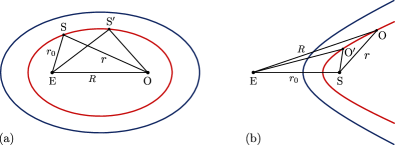
Figure 4: Lines of constant phase difference between the direct path $|EO|=R$ and the diffracted path $|ES|+|SO|=r_{0}+r$. Their shape is: (a) elliptic when the distance $R$ is fixed; (b) hyperbolic when $r_{0}$ is fixed.

However, for our case this zone construction is not convenient since (i) we have two image sources instead of one, and (ii) we are interested in just the opposite — in how to detect the scattering object due to the presence of wave effects in the observed signal, or in other words, where we should place the observer with the aim to detect the obstacle by virtue of diffraction with the highest efficiency. To this purpose we fix the points $E$ and $S$, while the observer $O$ is moved over the space [Fig. 4(b)]. By this procedure the line of constant phase difference between the two paths will be hyperbolic instead of elliptic (at the moment we assume a Minkowskian geometry).

V.2 Half plane

This idea can easily be implemented to our equations. First, consider the case of a single half plane with the geometry of Fig. 2. The penumbra term in Eq. (17) is determined by the Fresnel function of argument $w$, that depends on the path difference $d\equiv r+r_{0}-R$. Hence, one can define the zone structure by the condition that $d$ should be an integer number of half wavelengths:

$$r+r_{0}-\sqrt{r^{2}+r_{0}^{2}-2rr_{0}\cos\alpha}=\frac{\lambda}{2}\,j,$$ (24)

that means the phase between the paths changes by $\pi$ when moving from one zone to the next – a similar argument used by Fresnel to define the zone boundaries on the wavefront fresnel1821 ; crew1900 . From this equation, the shape of the zones in polar coordinates $(r,\alpha)$ will be determined by a familiar expression for conic sections

$$r=\frac{r_{0}}{2e_{j}}\,\frac{e_{j}^{2}-1}{1+e_{j}\cos\alpha}$$ (25)

with eccentricity $e_{j}$ given by

$$e_{j}\equiv\left(1-\frac{\lambda}{2r_{0}}\,j\right)^{-1}.$$ (26)

Eq. (25) describes a set of confocal hyperbolas (for $j=1,2,3,\dots$), all with the foci at the source $E$ and the edge of the screen $S$, so that the path difference from each focus to a point on the curve is constant [see Fig. 5(a)].

Figure 5: Lines of constant phase for the case of diffraction on a half-plane screen: (a) the source $E$ is at a distance $r_{0}$ from the edge $S$, the lines are hyperbolic; (b) the source is at infinity (plane wave incidence), they are parabolic.

Each hyperbola, in principle, should have two symmetrical branches corresponding to either $R>r$ or $R<r$. Since the latter case is not relevant for our physical conditions, we only consider the branches in the neighbourhood of the focus $S$ with $R>r$. Moreover, we are only interested in those parts of the branches which are located in the upper (illuminated) region where the direct and diffracted paths interfere. In the lower (shadowed) region no interference effects are expected since there is only the diffracted wave (this part is plotted in a dashed line). The vertices of the hyperbolas are given by the coordinates ($\frac{1}{4}\lambda j,0$), so that they are equidistantly spaced by $\frac{1}{4}\lambda$ between $r=0$ and $r=r_{0}/2$ along the screen. The asymptotes of the hyperbolas determine the limits for the angle $\alpha$ for each zone: $-\alpha_{j}^{*}<\alpha<\alpha_{j}^{*}$ with $\alpha_{j}^{*}=\arccos[-e_{j}^{-1}]$. We also notice that for our geometry, due to the requirement $1<e_{j}<\infty$ for hyperbolas, there is an upper limit for the index $j$ given by $j_{\rm max}=2r_{0}/\lambda$. Finally, for an infinitely distant source (incident plane wave), one focus goes to infinity, $r_{0}\to\infty$, and the path difference is simply $d=r(1+\cos\alpha)$, while the hyperbolas become parabolas with the single focus at the edge $S$ [see Fig. 5(b)]. The shape of the parabolas is determined by pla-string16

$$r=\frac{\lambda}{2}\,\frac{j}{1+\cos\alpha}.$$ (27)

V.3 String

Next, we consider the geometry of Fig. 1(b) corresponding to the string, which is flat space with a wedge removed and two sources located on the faces of the wedge. A qualitative analysis of Eq. (21) shows that in the most interesting situation, when the observer is in the double-imaging region, the diffraction pattern will be determined by the interference of four characteristic waves: two GO waves coming from the sources and two D waves emanating from the edge [Fig. 3(a)].

First of all, from geometrical optics we would expect the following picture: two GO waves interfering with each other, constructively or destructively, to produce an interference pattern of bright and dark lines alternating in space. The phase difference between the GO waves is constant along the lines: $s^{-}-s^{+}=const$, which are confocal hyperbolas with the foci at the sources $E^{-}$ and $E^{+}$. If we specify the path difference in units of the half wavelength:

$$s^{-}-s^{+}=\frac{\lambda}{2}\,q$$ (28)

with $q\in\mathbb{Z}$ being an integer, the bright lines (constructive interference) correspond to even $q=0,\pm 2,\pm 4,\dots$, while the dark lines (destructive interference) correspond to odd values $q=\pm 1,\pm 3,\dots$. In the following, we will refer to the bright and dark GO lines as “antinodal” and “nodal” lines, respectively.

The diffracted waves introduce new important features into the overall interference pattern. As we pointed out for the case of a half plane, the phase difference between the GO and D waves is constant along the hyperbolas: $r+r_{0}-s^{-}=const$, $r+r_{0}-s^{+}=const$, for the sources $E^{-}$ and $E^{+}$, respectively. The condition for destructive and constructive interference will now be different from that of Eq. (28). D waves acquire an additional phase shift of $3\pi/4$ by hitting the edge, which is manifested by virtue of the phase in the diffraction coefficients (22). Therefore, we would expect the maxima and minima of the field intensity when these two conditions are fulfilled simultaneously:

$$r+r_{0}-s^{+} =\frac{\lambda}{2}\,\left(n+\frac{3}{4}\right),$$ (29)

$$r+r_{0}-s^{-} =\frac{\lambda}{2}\,\left(m+\frac{3}{4}\right)$$ (30)

with $m,n$ being non-negative integers: $0,1,2,3,\dots$. The solutions are the intersection points of two families of hyperbolas corresponding to each source. If we now subtract Eqs. (29) and (30), we get Eq. (28) with $q=n-m$, that means these intersection points lie precisely on the nodal and antinodal GO lines. Therefore, we would expect that the additional interference with the D waves may lead to a further amplification of the field on the antinodal lines. The points of considerable interest are the global maxima, which occur when the two GO and the two D waves are all in phase, that corresponds to having all three numbers, $n$, $m$, and $q$, even. Denoting the intersection points by a pair of numbers $(n,m)$, the highest maximum occurs at the point $(0,0)$ which is located at the line of sight (central antinodal line). The next-order maxima are $(0,2)$ and $(2,0)$ lying symmetrically out of the line of sight at a larger distance from the string and having, therefore, lower magnitude. They are followed by more distant maxima $(0,4)$, $(2,2)$, $(4,0)$, and so on (see Fig. 6). An important special case occurs when $n$ and $m$ are odd simultaneously (accordingly $q$ is even). These are the saddle points of the field intensity which are located at the antinodal GO lines, e.g., $(1,1)$, $(3,1)$, $(1,3)$, etc. On the other hand, on the nodal lines, D waves do not substantially affect the wave field intensity due to the destructive interference between the GO waves.

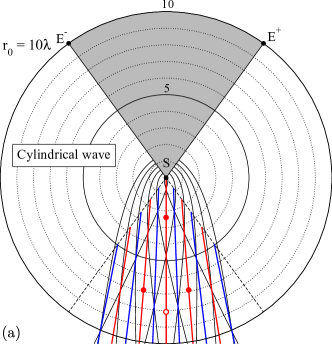
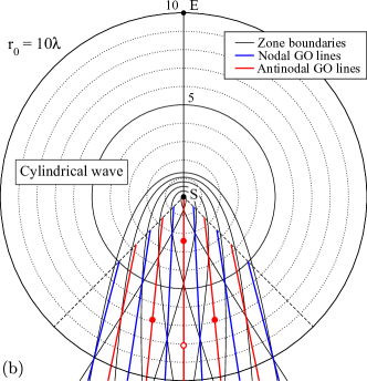
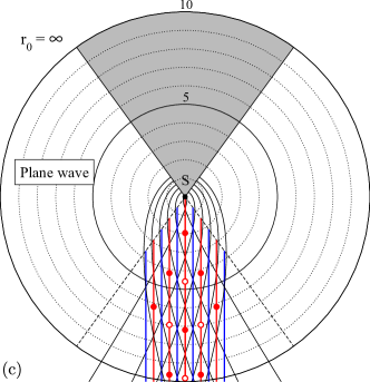
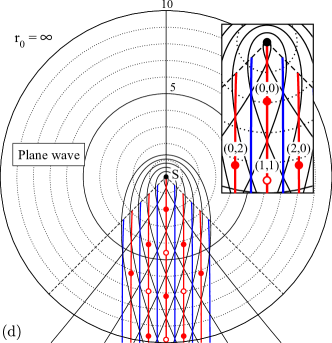
Figure 6: Observation zones associated with interference and diffraction of waves by a cosmic string: (a),(b) the source $E$ is at a finite distance $r_{0}$ from the string $S$; (c),(d) the source is at infinity (incident plane wave). Each case is shown for two coordinate systems: (a),(c) Minkowskian (2) with a wedge removed, and (b),(d) the one corresponding to Eq. (1). For a better view, a rather large value $\Delta=0.2\pi$ is taken. Dashed lines indicate the limits of the double-imaging region. Red points are the maxima of the field intensity, while red circles correspond to saddle points. Inset in (d): the points are labelled with $(n,m)$ indices.

For further analysis, one can define the observation zones, $\mathcal{Z}_{nm}$, associated with the points $(n,m)$, which are characteristic points of interference between the GO and D waves. Since an increase by 1 in indices corresponds to changes by $\pi$ in phase, we define the zones as delimited by the hyperbolic lines (29) and (30) with the substitution: $n\rightarrow n\pm\frac{1}{2}$ and $m\rightarrow m\pm\frac{1}{2}$. We call $\mathcal{Z}_{nm}$ as “Fresnel observation zones”, since the zone structure is basically determined by Fresnel diffraction. The zone boundaries can be defined explicitly by the hyperbolas (see Eq. (25) for comparison):

$$r=\frac{r_{0}}{2e_{j}}\,\frac{e_{j}^{2}-1}{1-e_{j}\cos(\Delta\pm\theta)}$$ (31)

with eccentricity

$$e_{j}=\left[1-\frac{\lambda}{2r_{0}}\,\left(j+\frac{3}{4}\right)\right]^{-1}.$$ (32)

For each zone $\mathcal{Z}_{nm}$ we have to substitute: $j=n-\frac{1}{2};\,n+\frac{1}{2}$ for the upper sign, $j=m-\frac{1}{2};\,m+\frac{1}{2}$ for the lower sign in Eq. (31). (Two different signs refer to the image sources $E^{\pm}$). The structure of Fresnel observation zones is depicted in Fig. 6. Here, the hyperbolas (31) are shown in black along with the GO antinodal (in red) and nodal (in blue) lines. Note that the interference between the GO waves takes place only in the double-imaging sector (bounded by dashes). Outside of it, the wave field is determined by interference of one GO and two D waves. Therefore, one would expect in the single-imaging region, the bright (antinodal) and dark (nodal) lines to be given by Eq. (29) to the right, and Eq. (30) to the left of the string location.

For an infinitely distant source, $r_{0}\to\infty$, the plane-wave approximation for the incident wave is held. Fig. 6(c),(d) shows the corresponding Fresnel-zone structure. In this case, the antinodal and nodal GO lines of Eq. (28) simply become straight lines parallel to the line of sight and given by

$$2r\sin\theta\,\sin\Delta=\frac{\lambda}{2}\,q$$ (33)

with $q$ being an integer. One can see that the separation between these lines is constant. This means that the typical fringe separation in the observation plane is $\lambda/(2\,\sin\Delta)\approx\lambda/(2\Delta)$, which is independent of the distance (even in space (1) whenever $\Delta\ll 1$). This is different from what happens in the diffraction by a compact object nakamura98 . For plane waves, the lines of constant phase between the GO and D waves become parabolas pla-string16 : $r[1-\cos(\Delta\pm\theta)]=const$. On the other hand, the phase shift in diffraction coefficients does not change when the source goes to infinity, therefore the conditions to find the maxima and minima will be similar to Eqs. (29) and (30), in which the indices $n$ and $m$ will identify the intersections of the parabolas. Since parabolas are the conic sections with eccentricity $e=1$, the parabolic Fresnel zones will be determined simply by

$$r=\frac{\lambda}{2}\,\frac{j+3/4}{1-\cos(\Delta\pm\theta)}$$ (34)

with $j$ defined below Eq. (32). These zones are depicted in Fig. 6(c). Finally, in order to obtain the observation zones in space (1), the angular transformation $\theta=\beta\varphi$ should be performed. As shown in Fig. 6(b),(d), this angular stretching distorts somewhat the shape of the curves, particularly as the angle increases. On the string’s line of sight ($\theta$=$\varphi$=$0$), however, the boundaries between the zones, as well as the maxima, coincide for both backgrounds (see Fig. 6).

The construction of Fresnel zones can also be carried out for other geometries. For instance, one can study a three-dimensional case with a point source emitting spherical waves, for which the analytical formulas for diffraction on a half plane are also known macdonald ; bowman69 . The surfaces of constant phase between the GO and D waves, though with more involved shapes, can also be obtained. To find the global diffraction maxima, what is needed is the value of the phase shift acquired by the D wave when hitting the string following the shortest path. It does not depend on the type of incident wave but on the obstacle keller62 ; kouyoumijan74 , having the value of $3\pi/4$ we have found for the conical space (1). We also note that for a far distant source, one can neglect the curvature of the wavefront and use the plane-wave approximation. In this limit, we expect the Fresnel zones to be hyperbolic cylinders having one focus on the string and the position of the other will depend on the tilted angle of incidence. In case of perpendicular incidence, the cylinders will become parabolic.

VI Discussion of the results

The zone structure we have introduced by simple analysis of four-wave interference is based on the geometrical theory of diffraction prescribed by Eq. (21). In spite of its asymptotic character, this theory is known to fit almost perfectly the exact solution in the diffraction experiments on obstacles as small as two wavelengths, with good predictions down to one wavelength [see, e.g., Ref. kapany65 ].

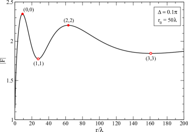
Figure 7: Amplification factor vs distance $r$ when the string is on the line of sight (central antinodal line). Intersection points of the hyperbolas are labelled.

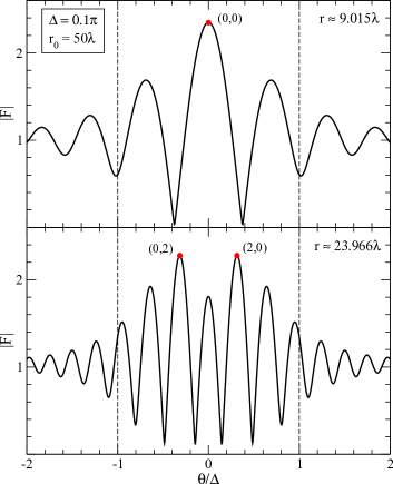
Figure 8: Amplification factor vs angular coordinate $\theta$ normalized to $\Delta$ for fixed distances from the string: (a) $r\approx 9.015\lambda$ corresponding to the position of $(0,0)$; (b) $r\approx 23.966\lambda$ corresponding to the location of $(2,0)$ and $(0,2)$. The boundaries of the double-imaging region are indicated by dashes.

We therefore believe that one can predict the location of the diffraction maxima due to wave scattering on the cosmic string with very high accuracy by a simple procedure described in Sect. V.3. For instance, to find the maximum $(n,m)$ corresponding to the zone $\mathcal{Z}_{nm}$, all we need is to calculate the crossing point of the two hyperbolas given by Eq. (31) with $j=n$ and $j=m$ for the two sources, respectively. This determines at which distance $r$ and angle $\theta$ from the string the point of maximum intensity should appear. To confirm our finding, Figs. 7 and 8 plot the modulus of the amplification factor $F$=$U/U_{0}$ calculated from the uniform asymptotics (19), which is more accurate than the geometrical theory of diffraction. The case when the string is on the line of sight, that corresponds to the observer on the central antinodal line ($\theta=0$), is depicted in Fig. 7. The intersection points of the hyperbolas, $(n,m)$, are seen to coincide precisely with the maxima and minima of the oscillations. Another case when the distance $r$ is fixed and the angular coordinate $\theta$ is varied is shown in Fig. 8. Again, we obtain a good correspondence between the exact values and the points given by the hyperbolas. The maxima and minima here correspond to the antinodal and nodal lines, respectively, originated from interference of two GO waves. They all could also be determined analytically by using Eq. (28).

Let us analyse the line-of-sight case in more detail. Due to the symmetry, the GO paths from the two sources are equal, $s^{-}=s^{+}\equiv s$. Therefore, the path difference between the GO and D waves is also identical for both sources and equal to $r+r_{0}-s$. From the uniform solution (19) we obtain the amplification factor at $\theta=0$ in the form

$$\left.F\right|_{\theta=0}=2\sqrt{\gamma}\,\mathrm{e}^{-\mathrm{i}\psi}\mathcal{F}(\sqrt{\psi})+\frac{\mathrm{e}^{\mathrm{i}\pi/4}}{\sqrt{\pi\psi}}\left(\sqrt{\gamma}-\sqrt{\frac{2\gamma}{\gamma+1}}\right),$$ (35)

which is a function of only two parameters: $\gamma\equiv(r+r_{0})/s$ and $\psi\equiv k(r+r_{0}-s)$. Taking into account that $0\leq\Delta\leq\pi/2$, it can be seen that $\gamma$ only ranges from 1 to $\sqrt{2}$. In the plane-wave limit, $r_{0}\to\infty$, one gets $\gamma\to 1$ and recovers the result of our previous work pla-string16 : $F=2\,\mathrm{e}^{-\mathrm{i}\psi}\mathcal{F}(\sqrt{\psi})$. A simpler formula can be obtained by expanding the Fresnel integral $\mathcal{F}$ in Eq. (35). For the modulus of the amplification we obtain

$$|F|_{\theta=0}\approx 2\sqrt{\gamma}\left[1-\frac{\sqrt{2}}{\sqrt{\pi\psi(\gamma+1)}}\cos{\left(\psi+\frac{\pi}{4}\right)}\right]^{1/2},$$ (36)

which is similar to the case of a plane-wave diffraction pla-string16 , but now the function oscillates around the GO value $|F_{\rm GO}|=2\sqrt{\gamma}$, that can be higher than 2.

Note that Eqs. (35) and (36) are also valid for large values of the conical parameter $\Delta$. It would be interesting to analyse the limit $\Delta\ll 1$, since the string scenario for galaxy formation requires a small deficit angle vilenkin-shellard94 . In this case, $\gamma\approx 1$ and $\psi\approx\pi\Delta^{2}\bar{r}/\lambda$, where $\bar{r}=rr_{0}/(r+r_{0})$ is a combination of the two characteristic distances. When the source goes to infinity, obviously $\bar{r}=r$, and the plane-wave limit is recovered (see Eq. (16) in Ref. pla-string16 ).

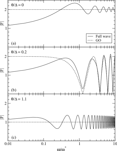
Figure 9: Amplification factor and its geometrical-optics limit vs frequency $\omega$ for three different angular positions $\theta$ of the observer: (a) line of sight; (b) double-imaging region, off line-of-sight; (c) single-imaging region. Plane-wave incidence on a string with $\Delta\ll 1$ is assumed.. The normalization frequency is $\omega^{*}\approx 2\pi c/(r\Delta^{2})$.

Next, consider the situation when the source, string, and observer occupy fixed positions. In this case the diffraction pattern can still in principle be observed in the energy (frequency) spectrum of the detected signal, since interference and diffraction are wavelength dependent. Several authors pointed out on such a possibility when they studied the interference effects in gravitational lensing by compact objects [see, e.g., Ref. peterson91 ; gould92 ]. What one would expect is the characteristic intensity modulation over the frequency spectrum. However, if the lensing object moves, the path-length differences will change with time, and the intensity oscillations (the maxima and the nodes) will move across the spectrum peterson91 ; gould92 . Let us analyse in the frequency domain the results we have obtained for the diffraction by the string. We will focus on the case of an infinitely distant source for simplicity. In this case, the wave field is

$$U=\mathrm{e}^{\mathrm{i}kr\cos(\Delta+\theta)}\mathcal{F}(w^{+})+\mathrm{e}^{\mathrm{i}kr\cos(\Delta-\theta)}\mathcal{F}(w^{-}),$$ (37)

with $w^{\pm}=\sqrt{2kr}\sin[(\Delta\pm\theta)/2]$, while in the GO limit, one should substitute in Eq. (37) $\mathcal{F}(w^{\pm})\to\mathcal{H}(\Delta\pm\theta)$ that gives two plane waves. Depending on the angular position $\theta$ of the observer, different kinds of patterns can be distinguished as shown in Fig. 9, where the modulus of the amplification factor is plotted as a function of frequency. We normalize the frequency for convenience by the value $\omega^{*}=\pi c/[r(1-\cos\Delta)]$ with $c$ being the speed of the wave. In such a way, the same plots are applicable when the coordinate $r$ of the observer is varied. From the experimental point of view, one can obtain information about the string’s parameters by matching the frequency pattern of the detected signal with one of the plots corresponding to different alignments and finding the characteristic $\omega^{*}$. In the limit $\Delta\ll 1$, this frequency is simply $\omega^{*}\approx 2\pi c/(r\Delta^{2})$.

Another distinctive feature is the magnitude of the amplification. The case of considerable interest is when the source, the string and the observer are all aligned ($\theta=0$). Given that the observer is on the central antinodal line and the interference between two GO waves is constructive for any $\omega$, the amplification factor in this case oscillates around the value $|F_{\rm GO}|=2$, approaching it at high frequencies [Fig. 9(a)]. The oscillations are due to interference between the GO and D waves, meaning that diffraction can increase the amplification to the values higher than 2. The highest maximum is about $2.34$ independently of the parameters pla-string16 . When the string is off the line-of-sight, but the observer is in the double-imaging region ($-\Delta<\theta<\Delta$), the oscillations become more profound ranging approximately between 0 and 2 [see Fig. 9(b)]. They appear due to more complex four-wave interference involving two GO and two D waves. Notice that the variation in frequency when the observation point is fixed is in some sense equivalent to the change in the distance $r$ with fixed $\theta$ and $\omega$. For the latter, the oscillations correspond to crossing the nodal and antinodal lines when $r$ increases [see Fig. 6(c)]. Finally, for the single-imaging region ($|\theta|>\Delta$) one of the sources is shadowed and $|F|$ oscillates around $|F_{\rm GO}|=1$. These oscillations are due to interference of one GO wave and two D waves [Fig. 9(c)].

VII Conclusions

We have presented an analytical theory that describes the propagation of scalar waves emitted by a source, which is located at a finite distance from a straight cosmic string, – a linear topological defect of spacetime. We show that the wave effects – interference and diffraction – are of importance and can be used to identify the string from other cosmological gravitational-lens objects. For a two-dimensional geometry, we have defined the Fresnel observation zones $\mathcal{Z}_{nm}$ bounded by conic sections: hyperbolas when a source is at finite distance, and parabolas for an infinitely distant source. Our theory allows to predict the location of the diffraction maxima, which are characteristic points of interference between the geometrical-optics and diffraction waves, corresponding to a specific observation zone. Additionally, one can obtain information about the string by matching the frequency pattern of the detected signal with theoretical plots corresponding to different alignments. Taking the typical value $\Delta\sim 10^{-7}$ and a distance to the string within our galaxy, $r\sim 10^{20}\,$m, one obtains the typical frequency $f^{*}\sim 100\,$Hz, which is in LIGO’s frequency band ligo16-2 . For larger distances, $r\sim 10^{26}\,$m, the frequency will be of the order $f^{*}\sim 10^{-4\,}$Hz, which is within the frequency range of Laser Interferometer Space Antenna (LISA) lisa16 . In the above discussion, it was assumed a static configuration of the lens system. If the string moves with respect to the observer-source line of sight, one would expect the wave amplification to be modulated in time at the observer’s position with a time scale $\sim r\Delta/c$. If the string moves with a relativistic velocity vilenkin-shellard94 , one obtains the time scale of the order of a week for the string moving at a distance $r\sim 10^{21}\,$m. On the other hand, the diffraction pattern will move across the frequency spectrum peterson91 ; gould92 . The latter effect will probably be more difficult to observe, since limited information on the whole spectrum could be collected during the sweep time.

We emphasize the difference between the usual diffraction on a physical obstacle (e.g., thin wire or slit) and the diffraction by a topological defect like a cosmic string. For the former, the diffraction oscillation pattern occurs near the shadow lines sommerfeld54 , while for the latter, there is no shadow at all, – the diffraction pattern appears due to the curvature of spacetime caused by the topology. We believe that our results are also applicable for condensed matter systems with similar underlying spacetime geometry. For instance, in nematic liquid crystals the linear topological defects are disclinations with a broader range of values of the conical parameter $\Delta$ pereira13 . It would be interesting to extend this method to other geometries or types of topological defects.

IFN acknowledges financial support from Universitat de Barcelona under the APIF scholarship.

References

- (1) B. P. Abbott, R. Abbott, T. D. Abbott et al., Phys. Rev. Lett. 116, 061102 (2016).
- (2) T. W. B. Kibble, J. Phys. A 9, 1387 (1976).
- (3) A. Vilenkin and E. P. S. Shellard, Cosmic Strings and Other Topological Defects (Cambridge University Press, Cambridge, 1994).
- (4) S. Deguchi and W. D. Watson, Phys. Rev. D 34, 1708 (1986).
- (5) I. Fernández-Núñez and O. Bulashenko, Phys. Lett. A 380, 2897 (2016).
- (6) A. Vilenkin, Phys. Rev. D 23, 852 (1981).
- (7) A. Vilenkin, Astrophys. J. 282, L51 (1984).
- (8) J. R. Gott, Astrophys. J. 288, 422 (1985).
- (9) T. T. Nakamura, Phys. Rev. Lett. 80, 1138 (1998).
- (10) A. Sommerfeld, Lectures on Theoretical Physics, Vol. IV, Optics (Academic Press, New York, 1954).
- (11) M. Born and E. Wolf, Principles of Optics, 7th ed. (Cambridge University Press, Cambridge, 1999).
- (12) D. S. Ahluwalia, R. M. Lewis, and J. Boersma, SIAM J. Appl. Math. 16, 783 (1968).
- (13) V. A. Borovikov and B. Ye. Kinber, Geometrical Theory of Diffraction, (The Institution of Electrical Engineers, London, 1994).
- (14) J. B. Keller, J. Opt. Soc. Am. 52, 116 (1962).
- (15) B. Linet, Ann. Inst. Henri Poincare A 45, 249 (1986).
- (16) T. Suyama, T. Tanaka, and R. Takahashi, Phys. Rev. D 73, 024026 (2006).
- (17) C. W. Misner and K. S. Thorne, and J. A. Wheeler, Gravitation (W. H. Freeman and Company, San Francisco, 1973).
- (18) H. M. Macdonald, Proc. London Math. Soc. 14, 140 (1915).
- (19) P. C. Clemmow, Quart. Journ. Mech. and Applied Math. 3, 377 (1950).
- (20) J. J. Bowman, T. B. A. Senior, and P. L. E. Uslenghi, Electromagnetic Acoustic Scattering by Simple Shapes, (North-Holland Publishing Company, Amsterdam, 1969).
- (21) R. G. Kouyoumijan and P. H. Pathak, Proc. IEEE 62, 1448 (1974).
- (22) A. Fresnel, Mèm. Acad. Sci. 5, 339 (1821).
- (23) The Wave Theory of Light: Memoirs of Huygens, Young and Fresnel, ed. by H. Crew, (American Book Company, New York, 1900), pp. 79–144.
- (24) H. L. Bertoni, Radio Propagation for Modern Wireless Systems (Prentice Hall, 1999).
- (25) P. Schneider, J. Ehlers, and E. Falco, Gravitational Lenses (Springer, New York, 1992).
- (26) T.T. Nakamura and S. Deguchi Prog. Theor. Phys. Suppl. 133, 137 (1999).
- (27) C.-M. Yoo, R. Saito, Y. Sendouda, K. Takahashi, and D. Yamauchi, Prog. Theor. Exp. Phys. 013E01 (2013).
- (28) N. S. Kapany, J. J. Burke, and K. Frame , Appl. Optics, 4, 1229 (1965).
- (29) J.B. Peterson, T. Falk, Astrophys. J. 374, L5 (1991).
- (30) A. Gould, Astrophys. J. 386, L5 (1992).
- (31) B. P. Abbott, et al. (The LIGO Scientific Collaboration), arXiv:1602.03845 (2016).
- (32) C. Caprini, M. Hindmarsh, S. Huber, et al., J. Cosmol. Astropart. Phys. 2016, No. 04, 001 (2016).
- (33) E. Pereira, S. Fumeron, and F. Moraes, Phys. Rev. E 87, 022506 (2013).