Nonlinearity in the sequential absorption of multiple photons

Abstract

I classify multiphoton absorption into separable, linked, and simultaneous processes. The first and second types can be distinguished when the rate-equation approximation is valid whereas the third type refers to the case when the full description of multiphoton absorption is essential. For this purpose, rate equations are solved analytically without decay processes which shows that even if many photons are absorbed the interaction with the light field is linear and one has the case of separable multiphoton absorption. Next a short-pulse approximation is investigated in which I first solve the rate equations without decay processes and then solve only rate equations for the ensuing decay. Finally, the full rate equations are examined and a successive approximation of the underlying Volterra integral equation of the second kind is derived leading to linked multiphoton absorption by the involved decay widths. The three methods are applied to a nitrogen atom in intense and ultrafast x rays from free-electron lasers (FELs). The linearity theorem barely approximates the results in the presence of decay processes which is also not satisfactorily corrected for by the short-pulse approximation. The successive approximation gives excellent agreement with the numerically-exact solution of the rate equations.

I Introduction

Rate equations which are systems of linear first-order ordinary differential equations Walter (2000) have recently come into focus in the study of the intense and ultrafast interaction of x rays with matter [e.g., Refs. Rohringer and Santra, 2007; Son, Young, and Santra, 2011a; *Son:EH-11; Buth et al., 2012; Son and Santra, 2012; *Son:EM-15; Rudek et al., 2012, 2013; Fukuzawa et al., 2013; Ho et al., 2014; Liu et al., 2016; Buth et al., 2017] due to the development of x-ray lasers, especially the state-of-the-art x-ray FELs such as the the Linac Coherent Light Source (LCLS) Arthur et al. (2002); Emma et al. (2010) in Menlo Park, California, USA, the SPring-8 Angstrom Compact free electron LAser (SACLA) Ishikawa et al. (2012) in Sayo-cho, Sayo-gun, Hyogo, Japan, the SwissFEL Ganter (2012) in Villigen, Switzerland, and the European X-Ray Free-Electron Laser (XFEL) Altarelli et al. (2006) in Hamburg, Germany. Such rate equations have been used for a long time in the optical regime L’Huillier et al. (1983a, b, c); Crance and Aymar (1985); Lambropoulos and Tang (1987); Delone and Krainov (2000) and, meanwhile, they have become frequently the basis for an understanding of the interaction with x rays, Rohringer and Santra (2007); Hoener et al. (2010); Young et al. (2010); Son, Young, and Santra (2011a); *Son:EH-11; Buth et al. (2012); Liu et al. (2016); Buth et al. (2017); Obaid et al. (2017) even in the presence of resonances, Xiang et al. (2012); Rudek et al. (2012, 2013); Fukuzawa et al. (2013); Ho et al. (2014) until coherent phenomena become important. Rohringer and Santra (2008a); *Rohringer:PN-08; Kanter et al. (2011); Cavaletto et al. (2012, 2013); Adams et al. (2013); Cavaletto et al. (2014); Li et al. (2016) This approach is required as the x rays from FELs are so intense that multiple x rays can be absorbed in the course of the interaction unlike experiments at synchrotrons which are limited to one-x-ray-photon processes. Als-Nielsen and McMorrow (2001); Adams et al. (2013) Hence—although the interaction with the x rays remains well-described by few-photon absorption cross sections in the cases considered for this work Makris, Lambropoulos, and Mihelič (2009)—a perturbative treatment of the interaction of the x-ray pulse with matter is typically no longer a viable approach as there is a substantial ground-state depletion.

In x-ray science the term “multiphoton absorption” is frequently used to refer to the case of the sequential absorption of several photons [e.g., Refs. Rohringer and Santra, 2007; Makris, Lambropoulos, and Mihelič, 2009; Hoener et al., 2010; Young et al., 2010; Son, Young, and Santra, 2011a; *Son:EH-11; Buth et al., 2012; Son and Santra, 2012; *Son:EM-15; Liu et al., 2016; Buth et al., 2017; Obaid et al., 2017] whereas for optical light predominantly the simultaneous absorption of several photons is meant. Delone and Krainov (2000) The attribute simultaneous, thereby, refers to the fact that a few-photon absorption cannot be meaningfully broken up into isolated photon absorption events with a smaller number of photons. X-ray absorption may occur either non-resonantly Rohringer and Santra (2007); Young et al. (2010); Son, Young, and Santra (2011a); *Son:EH-11; Buth et al. (2012); Liu et al. (2016); Buth et al. (2017); Obaid et al. (2017) or resonantly-enhanced. Xiang et al. (2012); Son and Santra (2012); *Son:EM-15; Rudek et al. (2012, 2013); Fukuzawa et al. (2013); Ho et al. (2014) The latter refers to a form of resonance-enhanced multiphoton ionization (REMPI) Delone and Krainov (2000) which is termed in this context resonance-enabled x-ray multiple ionization (REXMI). Rudek et al. (2012, 2013) Unlike optical photons, x rays typically have enough energy to eject electrons from atoms until maybe the highest charge states where simultaneous absorption of multiple x rays plays only a diminishing role. Doumy et al. (2011); Tamasaku et al. (2014)

In many applications, the x-ray energy is far above the ionization threshold of the involved atoms in all charge states such as in structure determination of biomolecules Neutze et al. (2000) and condensed matter. Als-Nielsen and McMorrow (2001) This is the case I focus on in this study. It is also what was examined in the initial works on matter in FEL x rays, e.g., Refs. Hoener et al., 2010; Young et al., 2010; Cryan et al., 2010; Fang et al., 2010, 2012. There the population of charge states due to ionization by the sequential absorption of multiple x rays and ensuing electronic decay processes are investigated by numerically solving rate equations. Rohringer and Santra (2007); Son, Young, and Santra (2011a); *Son:EH-11; Buth et al. (2012); Son and Santra (2012); *Son:EM-15; Liu et al. (2016); Buth et al. (2017) The solutions are then used to compute experimentally accessible quantities such as ion yields. Yet a more formal treatment of the underlying systems of differential equations has not been pursued to date.

Here I would like to investigate the solution of such rate equations analytically. I formulate and prove the linearity theorem of multiphoton absorption,  a short-pulse approximation that uses this theorem with decay equations, and I investigate the successive approximation of the solution of the rate equations. This allows me to classify multiphoton absorption into simultaneous, linked, and separable processes. Namely, specialized to a two-photon process, there is the well-known simultaneous absorption of two photons Göppert-Mayer (1931) for x rays. Rohringer and Santra (2007); Doumy et al. (2011) This changes when the rate-equation approximation without simultaneous two-photon terms is applicable. L’Huillier et al. (1983a, b, c); Crance and Aymar (1985); Lambropoulos and Tang (1987); Delone and Krainov (2000); Rohringer and Santra (2007); Makris, Lambropoulos, and Mihelič (2009); Buth et al. (2012, 2017) Then linked two-x-ray-photon absorption can be discussed where decay widths establish the link between two distinct one-x-ray-photon absorptions. In this article, I also turn to the third case of separable multiphoton absorption hitherto not analyzed which is covered by the linearity theorem. The reader should always bear in mind that linked and separable multiphoton absorption are approximations to simultaneous absorption. The core results of this article can be found in Sec. III where the analytical solution of the rate equations with decay are determined; Sec. II serves as an introduction to the subject neglecting decay processes.

This article is structured as follows. Section II treats rate equations without decay processes which are introduced in Sec. II.1. The linearity theorem of multiphoton absorption is proven in Sec. II.2. Rate equations with decay processes are treated in Sec. III; they are formulated in Sec. III.1. In Sec. III.2, I examine rate equations with decay processes in a short-pulse approximation. Section III.3 contains the derivation of a Volterra integral equation from the rate equations with decay and its successive approximation. Results and discussions are in Sec. IV where the time evolution of the charge states of a nitrogen is predicted using the approximations derived before. Conclusions are drawn in Sec. V.

Equations are formulated in atomic units. Hartree (1928); Szabo and Ostlund (1989) All details of the calculations in this article are provided in the Supplementary Data. Sup

II Rate equations without decay processes

II.1 Closed system of rate equations

I set out from rate equations which describe x-ray nonlinear optical processes of atoms Rohringer and Santra (2007); Buth et al. (2012, 2017) and molecules. Buth et al. (2012); Liu et al. (2016) The discussion is restricted to the case that the x-ray energy is sufficiently high to ionized all electrons of the atom by one-photon absorption.  The systems are assumed to be initially neutral with $N\in\mathbb{N}$ electrons and in a nondegenerate ground state. The electronic configurations of the system are enumerated by a double index of the electron number $n\in\{0,\ldots,N\}$ and the number of configurations $K^{(n)}\in\mathbb{N}$ in charge state $n$. The configurations are arranged with decreasing energy of configurations in each charge state. In total there are $K=\sum\limits_{n=0}^{N}K^{(n)}$ configurations. There is only one neutral state and one electron-bare state, i.e., $K^{(0)}=K^{(N)}=1$. For ease of notation, I let $K^{(N+1)}=0$. With x-ray flux $J$ I denote a continuous real function in time which is greater than zero only on a finite time interval and zero otherwise. With $\sigma_{j\leftarrow i}^{(n)},\sigma_{i}^{(n)}\geq 0$ for $i\in\{1,\ldots,K^{(n)}\}$, $j\in\{1,\ldots,K^{(n-1)}\}$, and $n\in\{0,\ldots,N\}$, I specify one-x-ray-photon absorption cross sections, partial and total cross sections, respectively.  Here $\sigma_{j\leftarrow i}^{(n)}$ is the cross section to transition from a configuration $i$ with $n$ electrons to a configuration $j$ with $n-1$ electrons by one-x-ray-photon absorption. Typically not all configurations $j$ can be reached from configuration $i$ and $\sigma_{j\leftarrow i}^{(n)}$ is set to zero, if it is not possible. For notational convenience, I let $\sigma_{j\leftarrow 1}^{(0)}=\sigma_{1\leftarrow i}^{(N+1)}=0$ for any $i$, $j$. The $\sigma_{i}^{(n)}$ is the cross section to transition from configuration $i$ with $n$ electrons to any accessible configuration with $n-1$ electrons. As no x rays can be absorbed by the electron-bare nucleus, I have for this configuration $\sigma_{1}^{(0)}=0$.

Rate equations can be constructed as follows or be derived from the master equation in Lindblad form as a Pauli master equation which is discussed in Refs. Pauli, 1928; Louisell, 1990; Buth, 2017. Given probabilities Krengel (2005) $P_{j}^{(n)}(t)$ at time $t\in\mathbb{R}$ which are differentiable, to find the system at time $t\in\mathbb{R}$ with $n$ electrons in configuration $j$. The initial condition is specified at the initial time $\tau\in\mathbb{R}$ as $P_{j}^{(n)}(\tau)$. Here I assume further that the system is initially in the single neutral charge state, i.e., $P_{j}^{(n)}(\tau)=\delta_{1\,j}\,\delta_{N\,n}$ with the Kronecker-$\delta$. Kuptsov (originator) Then the first rate equation, for the system in its neutral charge state reads

$$\dfrac{\>\mathrm{d}P_{1}^{(N)}(t)}{\>\mathrm{d}t}=-\sigma_{1}^{(N)}\,P_{1}^{(N)}(t)\,J(t)\;;$$ (1)

it describes the ionization of the neutral system by the x rays. The rate equations of the singly-ionized system already have the full form of rate equations without decay processes

$$\dfrac{\>\mathrm{d}P_{j}^{(N-1)}(t)}{\>\mathrm{d}t}=\bigl{[}\sigma_{j\leftarrow 1}^{(N)}\;P_{1}^{(N)}(t)-\sigma_{j}^{(N-1)}\,P_{j}^{(N-1)}(t)\bigr{]}\,J(t)\;;$$ (2)

for $j\in\{1,\ldots,K^{(N-1)}\}$. This continues analogously until the last rate equation, for the electron-bare system, which is

$$\dfrac{\>\mathrm{d}P_{1}^{(0)}(t)}{\>\mathrm{d}t}=\sum\limits_{i=1}^{K^{(1)}}\sigma_{1\leftarrow i}^{(1)}\;P_{i}^{(1)}(t)\,J(t)\;.$$ (3)

The above said can be compactly summarized as follows. Inspecting the rate equations (1), (2), (3), I observe that there are $K$ rate equations which form the $K\times K$ system of linear first-order ordinary differential equations

$$\dfrac{\>\mathrm{d}P_{j}^{(n)}(t)}{\>\mathrm{d}t}=\Bigl{[}\sum\limits_{i=1}^{K^{(n+1)}}\sigma_{j\leftarrow i}^{(n+1)}\;P_{i}^{(n+1)}(t)-\sigma_{j}^{(n)}\,P_{j}^{(n)}(t)\Bigr{]}\,J(t)\;.$$ (4)

Then this constitutes a system of rate equations. If for such a system of rate equations the total cross sections are given by

$$\sigma_{j}^{(n)}=\sum\limits_{i=1}^{K^{(n-1)}}\sigma_{i\leftarrow j}^{(n)}\;,$$ (5)

then it is termed a closed system of rate equations.

The system of rate equations (4) for all $n$, $j$ can be rewritten compactly by letting $\hbox{\boldmath{$p$}\unboldmath}(t)\in\mathbb{R}^{K}$ stand for the vector with the entries $P_{i}^{(n)}(t)$, i.e.,

$$\hbox{\boldmath{$p$}\unboldmath}(t)=\bigr{(}P_{1}^{(N)}(t),P_{1}^{(N-1)}(t),\ldots,P_{K^{(N-1)}}^{(N-1)}(t),\ldots,P_{1}^{(0)}(t)\bigr{)}{}^{\textrm{\scriptsize T}}\;.$$ (6)

The partial cross sections $\sigma_{j\leftarrow i}^{(n)}$ form a strictly lower triangular matrix and $-\sigma_{i}^{(n)}$ are on the matrix diagonal. Together they are referred to as the cross section matrix $\Sigma$. With this notation, I express (4) as

$$\dfrac{\>\mathrm{d}\hbox{\boldmath{$p$}\unboldmath}(t)}{\>\mathrm{d}t}=\hbox{\boldmath{$\Sigma$}\unboldmath}\;\hbox{\boldmath{$p$}\unboldmath}(t)\,J(t)\;.$$ (7)

The structure of $\Sigma$ can be characterized by

Definition 1.

A real $K\times K$ matrix $A$ that has the closure property:

$$-A_{ii}=\sum\limits_{\genfrac{}{}{0.0pt}{}{\scriptstyle j=1}{\scriptstyle j\neq i}}^{K}A_{ji}\;,$$ (8)

for all $i\in\{1,\ldots,K\}$ is referred to as closed matrix.

The closure property (5) implies that $\Sigma$ in (7) is a closed matrix.

Remark 1.

If the matrix $A$ from Definition 1 is also lower-triangular, then it has at least one zero diagonal element because $A_{KK}=0$ must hold in order to fulfill (8).

So far I referred to the $p_{i}(t)$ as probabilities thereby assuming them to lie in $[0;1]$ for all times $t$. Krengel (2005) This fact, however, needs to be established rigorously.

Remark 2.

The $\Sigma$ is essentially nonnegative, i.e., $\Sigma_{ij}\geq 0$ for $i\neq j$, and thus a Metzler matrix. Giorgio and Zuccotti (2015) Therefore, Theorem 16.VII on page 183 in Ref. Walter, 2000 ensures the nonnegativity of the $p_{i}(t)$.

The word “closed” was chosen above to hint that

Lemma 1.

Probability in a closed system of rate equations (4) is conserved.

Proof.

As $\Sigma$ is a closed matrix (5), I observe that the column sums of $\Sigma$ vanish, i.e., $\sum\limits_{i=1}^{K}\Sigma_{ij}=0$ for all $j\in\{1,\ldots,K\}$. Then it follows by summing the components of (7):

$$\dfrac{\>\mathrm{d}}{\>\mathrm{d}t}\sum\limits_{i=1}^{K}p_{i}(t)=\sum\limits_{j=1}^{K}\Bigl{[}\sum\limits_{i=1}^{K}\Sigma_{ij}\Bigr{]}\;p_{j}(t)\,J(t)=0\;,$$ (9)

that the probability is conserved for all times $t$. ∎

Thus I make the

Remark 3.

With Remark 2 and Lemma 1 I can rightfully refer to the $p_{i}(t)$ as probabilities Krengel (2005) provided that the initial values fulfill $0\leq p_{i}(\tau)\leq 1$ for $i\in\{1,\ldots,K\}$ and $\sum\limits_{i=1}^{K}p_{i}(\tau)=1$ holds.

II.2 Linearity theorem of multiphoton absorption

The rate equations (7) constitute a matrix initial-value problem which satisfies the Lappo-Danilevskii condition Komlenko (originator):

$$\hbox{\boldmath{$\Sigma$}\unboldmath}\,J(t)\int\limits_{\tau}^{t}\hbox{\boldmath{$\Sigma$}\unboldmath}\,J(t^{\prime})\>\mathrm{d}t^{\prime}=\int\limits_{\tau}^{t}\hbox{\boldmath{$\Sigma$}\unboldmath}\,J(t^{\prime})\>\mathrm{d}t^{\prime}\>\hbox{\boldmath{$\Sigma$}\unboldmath}\,J(t)\;.$$ (10)

Hence the fundamental matrix can be written as an exponential function $\mathrm{e}^{\int\limits_{\tau}^{t}\hbox{\boldmath{$\scriptstyle{\Sigma}$}\unboldmath}\,J(t^{\prime})\>\mathrm{d}t^{\prime}}$ Komlenko (originator) which leads to the solution of the rate equations (7) on the last line of Eq. (II.2). But only some of the results in the following paragraphs are found this way.

To gain deeper insight into the physics described by the rate equations (7), I obtain the solution of (7) in an alternative way using the eigenbasis of $\Sigma$. For this I notice that, as $\Sigma$ is lower triangular, its eigenvalues are the diagonal elements $-\sigma_{i}^{(n)}$ which are negative or zero such as the last one $-\sigma_{1}^{(0)}=0$—because the electron-bare nucleus cannot be ionized further—and pairwise distinct as the total absorption cross sections $\sigma_{i}^{(n)}$ refer to different configurations $i$ of charge state $n$ where, on configuration level, there are no degeneracies. Following Lemma 2, $\Sigma$ is diagonalizable where the eigenvalues form the diagonal matrix $\hbox{\boldmath{$\Lambda$}\unboldmath}=\textbf{diag}(\lambda_{1},\ldots,\lambda_{K})$ and the eigenvectors are gathered in the matrix $U$. As $\Sigma$ is time independent, so are $\Lambda$ and $U$. Transforming (7) to the eigenbasis of $\Sigma$ yields

$$\hbox{\boldmath{$U$}\unboldmath}^{-1}\,\dfrac{\>\mathrm{d}\hbox{\boldmath{$p$}\unboldmath}(t)}{\>\mathrm{d}t} = \dfrac{\>\mathrm{d}\hbox{\boldmath{$q$}\unboldmath}(t)}{\>\mathrm{d}t}=\hbox{\boldmath{$U$}\unboldmath}^{-1}\,\hbox{\boldmath{$\Sigma$}\unboldmath}\,\hbox{\boldmath{$U$}\unboldmath}\;\hbox{\boldmath{$U$}\unboldmath}^{-1}\,\hbox{\boldmath{$p$}\unboldmath}(t)\,J(t)$$ (11)

$$= \hbox{\boldmath{$\Lambda$}\unboldmath}\,\hbox{\boldmath{$q$}\unboldmath}(t)\,J(t)\;,$$

which is a decoupled system of linear first-order ordinary differential equations. The $\ell$ th equation reads

$$\dfrac{\>\mathrm{d}q_{\ell}(t)}{\>\mathrm{d}t}=\lambda_{\ell}\,q_{\ell}(t)\,J(t)\;,$$ (12)

which has the solution for time $t\geq\tau$ with the integration starting at time $\tau$:

$$q_{\ell}(t)=q_{\ell}(\tau)\;\mathrm{e}^{\lambda_{\ell}\,\Phi(t)}\;,$$ (13)

where the initial value is $q_{\ell}(\tau)\equiv(\hbox{\boldmath{$U$}\unboldmath}^{-1}\,\hbox{\boldmath{$p$}\unboldmath}(\tau))_{\ell}$ and the x-ray fluence is

$$\Phi(t)=\int\limits_{\tau}^{t}J(t^{\prime})\>\mathrm{d}t^{\prime}\;.$$ (14)

As the system is initially in its ground state, I have $\hbox{\boldmath{$p$}\unboldmath}(\tau)=(1,0,\ldots,0){}^{\textrm{\scriptsize T}}\in\mathbb{R}^{K}$ and thus $q_{\ell}(\tau)=(\hbox{\boldmath{$U$}\unboldmath}^{-1})_{\ell 1}$. From the solution $\hbox{\boldmath{$q$}\unboldmath}(t)$, the probabilities follow via $\hbox{\boldmath{$p$}\unboldmath}(t)=\hbox{\boldmath{$U$}\unboldmath}\,\hbox{\boldmath{$q$}\unboldmath}(t)$, hence

$$p_{i}(t)=\sum\limits_{\ell=1}^{K}U_{i\ell}\,q_{\ell}(t)=\sum\limits_{\ell=1}^{K}U_{i\ell}\,q_{\ell}(\tau)\;\mathrm{e}^{-|\lambda_{\ell}|\,\Phi(t)}\;,$$ (15)

which is the unique solution of the system of rate equations (7).

I observe that $p_{i}(t)$ depends only on the x-ray fluence $\Phi(t)$ as it is the case for one-photon absorption. Buth et al. (2012) The sign of $\lambda_{\ell}$ in (13) was made explicit in (15); it implies that the exponential functions in (15) decay quickly to zero with increasing fluence meaning that the probability of the system at time $t$ to be in the configuration $i$ with electrons decays to zero such that for $\Phi(t)\to\infty$, eventually, only the last configuration $K$ of the system which is stripped bare of electrons, i.e., $\lambda_{K}=0$, has unit probability [see (9)]. Conversely, the limit $\Phi(t)\to 0$ lets all exponential functions in (15) become unity and thus $\hbox{\boldmath{$p$}\unboldmath}(t)=\hbox{\boldmath{$p$}\unboldmath}(\tau)$, i.e., the system remains in the initial state for all times $t$.

The solution (15) of the rate equations (7) is recast, by expanding the exponential function into a series using $\hbox{\boldmath{$q$}\unboldmath}(\tau)=\hbox{\boldmath{$U$}\unboldmath}^{-1}\,\hbox{\boldmath{$p$}\unboldmath}(\tau)$, yielding

$$p_{i}(t) = \sum\limits_{m=0}^{\infty}\dfrac{\Phi^{m}(t)}{m!}\sum\limits_{\ell,j=1}^{K}(\hbox{\boldmath{$U$}\unboldmath}^{\vphantom{-1}})_{i\ell}\,\lambda_{\ell}^{m}\,(\hbox{\boldmath{$U$}\unboldmath}^{-1})_{\ell j}\>p_{j}(\tau)$$

$$= \sum\limits_{j=1}^{K}p_{j}(\tau)\sum\limits_{m=0}^{\infty}\dfrac{\Phi^{m}(t)}{m!}\>\hbox{\boldmath{$\Sigma$}\unboldmath}^{m}_{ij}$$

$$= \sum\limits_{j=1}^{K}\bigl{(}\mathrm{e}^{\hbox{\boldmath{$\scriptstyle{\Sigma}$}\unboldmath}\,\Phi(t)}\bigr{)}_{ij}\;p_{j}(\tau)\;.$$

The middle expression in (II.2) exhibits the perturbative nature of the problem. Namely, the probability $\hbox{\boldmath{$p$}\unboldmath}(t)$ is composed of the summands with increasing powers of $\hbox{\boldmath{$\Sigma$}\unboldmath}\>\Phi(t)$, i.e., zero-photon absorption gives $\mathbbm{1}$, one-photon absorption adds $\hbox{\boldmath{$\Sigma$}\unboldmath}\>\Phi(t)$, two-photon absorption adds $\tfrac{1}{2}\,\bigl{(}\hbox{\boldmath{$\Sigma$}\unboldmath}\>\Phi(t)\bigr{)}^{2}$, …. The above said proves

Theorem 1 (Linearity theorem of multiphoton absorption).

Given a system of rate equations (4), then there is no nonlinearity in the interaction of x rays with the system and all multiphoton processes can be decomposed in terms of subsequent (chained) one-x-ray-photon absorptions (II.2).

The situation that is described by Theorem 1 is termed separable multiphoton absorption. The dependence of $\hbox{\boldmath{$p$}\unboldmath}(t)$ on $t$ is nonlinear due to the exponential functions in (15) that become constants which depend only on the x-ray fluence after the x-ray pulse has passed for $t\to\infty$. In the case of separable multiphoton processes, no nonlinearity in the interaction is present. The fact that the exponential series always converges ought not to mislead the reader: this convergence does not imply that the physical problem of multiphoton absorption actually is amenable to a perturbative treatment which leads to the cross sections that enter (4). This fact needs to be established independently. Sorokin et al. (2007); Makris, Lambropoulos, and Mihelič (2009)

III Rate equations with decay processes

III.1 Closed system of rate equations

In many cases the formulation of the rate equations (4) from Sec. II.1 represent an idealization because there are decay processes occurring. First, there is electronic decay in which an electron drops from a higher shell to a lower shell releasing the excess energy by ejecting another electron from a higher shell. Second, there is radiative decay where an electron drops from a higher shell to a lower shell emitting a photon with an energy corresponding to the energy difference between the two shells involved in the transition. For electronic decay, the final state has one electron less compared with the initial state whereas in radiative decay the number of electrons is left unchanged.

With decay widths, the rate equations (4) become

$$\dfrac{\>\mathrm{d}P_{j}^{(n)}(t)}{\>\mathrm{d}t} = \Bigl{[}\sum\limits_{i=1}^{K^{(n+1)}}\sigma_{j\leftarrow i}^{(n+1)}\;P_{i}^{(n+1)}(t)-\sigma_{j}^{(n)}\,P_{j}^{(n)}(t)\Bigr{]}\,J(t)$$

$${}+\sum\limits_{i=1}^{K^{(n+1)}}\gamma_{\mathrm{E},j\leftarrow i}^{(n+1)}\;P_{i}^{(n+1)}(t)$$

$${}+\sum\limits_{i=1}^{K^{(n)}}\gamma_{\mathrm{R},j\leftarrow i}^{(n)}\;P_{i}^{(n)}(t)$$

$${}-\gamma_{j}^{(n)}\,P_{j}^{(n)}(t)\;,$$

where the partial decay widths for electronic decay are $\gamma_{\mathrm{E},j\leftarrow i}^{(n+1)}\geq 0$ and for radiative decay are $\gamma_{\mathrm{R},j\leftarrow i}^{(n)}\geq 0$. Note that $\gamma_{\mathrm{R},j\leftarrow i}^{(n)}=0$ for $j\geq i$. The total decay width of a system in configuration $j$ with $n$ electrons to make a transition to any in this way accessible other configuration is $\gamma_{j}^{(n)}=\gamma_{\mathrm{E},j}^{(n)}+\gamma_{\mathrm{R},j}^{(n)}$ in analogy to (5) given by

$$\gamma_{\mathrm{E},j}^{(n)}=\sum\limits_{i=1}^{K^{(n-1)}}\gamma_{\mathrm{E},i\leftarrow j}^{(n)}\hbox{\quad and\quad}\gamma_{\mathrm{R},j}^{(n)}=\sum\limits_{i=1}^{K^{(n)}}\gamma_{\mathrm{R},i\leftarrow j}^{(n)}\;.$$ (18)

The decay widths $\gamma_{\mathrm{R},j\leftarrow i}^{(n)}$ and $\gamma_{j}^{(n)}$ make their first appearance in the rate equations for $n=N-1$, i.e., Eq. (2), and the $\gamma_{\mathrm{E},j\leftarrow i}^{(n)}$ start to appear in the rate equations for $n=N-2$. There is no decay in the first rate equation, for the system in its neutral charge state which has the same form as (1). The last rate equation, for the electron-bare system, similar to (3), also does not contain a decay width.

Introducing the notation of (6) and (7), I express (III.1) compactly as

$$\dfrac{\>\mathrm{d}\hbox{\boldmath{$\mathfrak{p}$}\unboldmath}(t)}{\>\mathrm{d}t}=\hbox{\boldmath{$\Sigma$}\unboldmath}\;\hbox{\boldmath{$\mathfrak{p}$}\unboldmath}(t)\,J(t)+\hbox{\boldmath{$\Gamma$}\unboldmath}\;\hbox{\boldmath{$\mathfrak{p}$}\unboldmath}(t)\;.$$ (19)

I have, additionally, the matrix of decay widths $\Gamma$. Because of the radiative decay widths, for this matrix to be lower triangular with the negative of the total decay widths on the diagonal, the electron configurations need to be sorted with decreasing energy. Further the first and last rows and column of $\Gamma$ are filled with zeros; the inner part shall be referred to by $\hbox{\boldmath{$\Gamma$}\unboldmath}^{\,\prime}$, i.e., $\Gamma$ can be written as the direct sum $\hbox{\boldmath{$\Gamma$}\unboldmath}=(0)\oplus\hbox{\boldmath{$\Gamma$}\unboldmath}^{\,\prime}\oplus(0)$. Due to the closure property (18), $\Gamma$ is a closed matrix and the probability Krengel (2005) in the system of rate equations (III.1) is conserved in analogy to Remarks 2 and 3 and Lemma 1.

III.2 Decay equation

Inspecting (19), I find that, with decay widths present, one cannot proceed any longer as for the case without decay widths. Namely, as $\Sigma$ and $\Gamma$, in general, do not commute, the Lappo-Danilevskii condition (10) is not fulfilled for $\hbox{\boldmath{$\Sigma$}\unboldmath}\,J(t)+\hbox{\boldmath{$\Gamma$}\unboldmath}$. For the same reason, the two matrices do not share a common eigenbasis, Fischer (2014); Sup i.e., the matrix on the right-hand side of (19) cannot be diagonalized by a time-independent matrix as in (11). Certainly, Equation (19) can be integrated numerically as in Ref. Buth et al., 2012 or solved using the analytical solutions of Sec. III.3 but here I would like to determine an approximate solution of it. I obtain the solution (15) of the rate equations neglecting the decay widths (7) first. Thereby, I assume that the x-ray pulse is so short that, in the course of the interaction, no noticeable decay of excited states occurs. Second, I solve (19) without cross sections, i.e., the decay equation:

$$\dfrac{\>\mathrm{d}\hbox{\boldmath{$\mathfrak{p}$}\unboldmath}(t)}{\>\mathrm{d}t}=\hbox{\boldmath{$\Gamma$}\unboldmath}\;\hbox{\boldmath{$\mathfrak{p}$}\unboldmath}(t)\;,$$ (20)

by going to the eigenbasis of $\Gamma$. Walter (2000) Namely, the decay widths for different electronic configurations of the system are pairwise distinct or zero; then, according to Lemma 2, the matrix $\Gamma$ is diagonalizable. Thus I have $\hbox{\boldmath{$\Gamma$}\unboldmath}=\hbox{\boldmath{$\mathfrak{U}$}\unboldmath}\,\hbox{\boldmath{$M$}\unboldmath}\,\hbox{\boldmath{$\mathfrak{U}$}\unboldmath}^{-1}$ with the matrix of eigenvectors $\mathfrak{U}$ and the matrix of eigenvalues $\hbox{\boldmath{$M$}\unboldmath}=\textbf{diag}(\mu_{1},\ldots,\mu_{K})$. I arrive at the decoupled system of differential equations of the decay

$$\hbox{\boldmath{$\mathfrak{U}$}\unboldmath}^{-1}\,\dfrac{\>\mathrm{d}\hbox{\boldmath{$\mathfrak{p}$}\unboldmath}(t)}{\>\mathrm{d}t}=\dfrac{\>\mathrm{d}\hbox{\boldmath{$\mathfrak{q}$}\unboldmath}(t)}{\>\mathrm{d}t}=\hbox{\boldmath{$M$}\unboldmath}\,\hbox{\boldmath{$\mathfrak{q}$}\unboldmath}(t)\;,$$ (21)

which has the solution with $1\leq\ell\leq K$, in analogy to (13), given by

$$\mathfrak{q}_{\ell}(t)=\mathfrak{q}_{\ell}(\mathfrak{T})\;\mathrm{e}^{\mu_{\ell}\,(t-\mathfrak{T})}\;.$$ (22)

Here decay is assumed to begin at time $\mathfrak{T}$. The starting probabilities at time $T$ are found from the solution of the system of rate equations without decay (15) and (II.2). They are $\hbox{\boldmath{$\mathfrak{p}$}\unboldmath}(\mathfrak{T})=\hbox{\boldmath{$p$}\unboldmath}(T)=\hbox{\boldmath{$\mathfrak{U}$}\unboldmath}\,\hbox{\boldmath{$\mathfrak{q}$}\unboldmath}(\mathfrak{T})\iff\hbox{\boldmath{$\mathfrak{q}$}\unboldmath}(\mathfrak{T})=\hbox{\boldmath{$\mathfrak{U}$}\unboldmath}^{-1}\,\hbox{\boldmath{$\mathfrak{p}$}\unboldmath}(\mathfrak{T})=\hbox{\boldmath{$\mathfrak{U}$}\unboldmath}^{-1}\,\hbox{\boldmath{$U$}\unboldmath}\,\hbox{\boldmath{$q$}\unboldmath}(T)$ where $\hbox{\boldmath{$q$}\unboldmath}(T)$ is given by (13). Nota bene, that not necessarily $\mathfrak{T}=T$ holds. I introduce this flexibility, to allow the decay equations to be integrated also from a $\mathfrak{T}$ as the onset time of decay processes.

The solution of the decay equations (22) is transformed back from the eigenbasis of $\Gamma$ to the original basis via

$$\mathfrak{p}_{i}(t) = \sum\limits_{\ell=1}^{K}\mathfrak{U}_{i\ell}\;\mathrm{e}^{\mu_{\ell}\,(t-\mathfrak{T})}\>\mathfrak{q}_{\ell}(\mathfrak{T})$$

$$= \sum\limits_{n=0}^{\infty}\sum\limits_{\ell,j=1}^{K}\mathfrak{U}_{i\ell}\,\mu_{\ell}^{n}\,(\hbox{\boldmath{$\mathfrak{U}$}\unboldmath}^{-1})_{\ell j}\,\dfrac{(t-\mathfrak{T})^{n}}{n!}\,\mathfrak{p}_{j}(\mathfrak{T})\;.$$

I arrive at the compact form of the solution into which the solution of the rate equations without decay (II.2) is inserted proving

Theorem 2.

The approximate solution of rate equations with decay processes (19) in terms of a solution of the rate equations without decay (7) in the time interval $[\tau;T]$ and subsequently the decay equation (20) reads

$$\hbox{\boldmath{$\mathfrak{p}$}\unboldmath}(t)=\mathrm{e}^{\hbox{\boldmath{$\scriptstyle{\Gamma}$}\unboldmath}\,(t-\mathfrak{T})}\>\hbox{\boldmath{$\mathfrak{p}$}\unboldmath}(\mathfrak{T})=\mathrm{e}^{\hbox{\boldmath{$\scriptstyle{\Gamma}$}\unboldmath}\,(t-\mathfrak{T})}\;\mathrm{e}^{\hbox{\boldmath{$\scriptstyle{\Sigma}$}\unboldmath}\,\Phi(T)}\>\hbox{\boldmath{$p$}\unboldmath}(\tau)\;,$$ (24)

for times $t\geq\mathfrak{T}$. Photoionization lasts till time $T$ and decay processes start at time $\mathfrak{T}$.

Theorem 2 does not reduce to Theorem 1 upon letting $\hbox{\boldmath{$\Gamma$}\unboldmath}=\hbox{\boldmath{$0$}\unboldmath}$ as the photoionization of the system is assumed to be completed at time $T$, i.e., the temporal progression of photoionization does not enter (24). This apparent weakness of Theorem 2, however, can be used judiciously by replacing the solution of the nondecaying system $\mathrm{e}^{\hbox{\boldmath{$\scriptstyle{\Sigma}$}\unboldmath}\,\Phi(T)}\>\hbox{\boldmath{$p$}\unboldmath}(\tau)$ by a (numerical) solution of (19) in the time interval $[\tau;T]$. In this case, the solution of Eq. (20), $\mathrm{e}^{\hbox{\boldmath{$\scriptstyle{\Gamma}$}\unboldmath}\,(t-\mathfrak{T})}\>\hbox{\boldmath{$p$}\unboldmath}(T)$ for $\mathfrak{T}=T$ and $t\geq T$, is the (numerically-)exact solution of (19). This procedure has been used to treat slow radiative decay to calculate photon yields in Ref. Buth et al., 2017.

III.3 Successive approximation

A simple analytic solution of the interacting and decaying system (19) in terms of the Peano-Baker series is well known Komlenko (originator); Baake and Schlägel (2011); it is stated in

Theorem 3.

Given a system of rate equations with decay (19), then its solution is

$$\hbox{\boldmath{$\mathfrak{p}$}\unboldmath}(t)=\hbox{\boldmath{$X$}\unboldmath}(t)\,\hbox{\boldmath{$\mathfrak{p}$}\unboldmath}(\tau)\;,$$ (25)

for times $t\geq\tau$ with the fundamental matrix Komlenko (originator):

$${}\hbox{\boldmath{$X$}\unboldmath}(t)=\hbox{\boldmath{$\mathbbm{1}$}\unboldmath}+\int\limits_{\tau}^{t}(\hbox{\boldmath{$\Sigma$}\unboldmath}\,J(t^{\prime})+\hbox{\boldmath{$\Gamma$}\unboldmath})\>\mathrm{d}t^{\prime}$$ (26)

$${}+\int\limits_{\tau}^{t}(\hbox{\boldmath{$\Sigma$}\unboldmath}\,J(t^{\prime})+\hbox{\boldmath{$\Gamma$}\unboldmath})\int\limits_{\tau}^{t^{\prime}}(\hbox{\boldmath{$\Sigma$}\unboldmath}\,J(t^{\prime\prime})+\hbox{\boldmath{$\Gamma$}\unboldmath})\>\mathrm{d}t^{\prime\prime}\>\mathrm{d}t^{\prime}$$

$${}+\ldots\;.$$

Proof.

The fundamental matrix $\hbox{\boldmath{$X$}\unboldmath}(t)$ solves the initial-value problem $\tfrac{\>\mathrm{d}\hbox{\boldmath{$\scriptstyle{X}$}\unboldmath}(t)}{\>\mathrm{d}t}=(\hbox{\boldmath{$\Sigma$}\unboldmath}\,J(t)+\hbox{\boldmath{$\Gamma$}\unboldmath})\,\hbox{\boldmath{$X$}\unboldmath}(t)$, $\hbox{\boldmath{$X$}\unboldmath}(\tau)=\hbox{\boldmath{$\mathbbm{1}$}\unboldmath}$. Komlenko (originator) This equation can be integrated leading to $\hbox{\boldmath{$X$}\unboldmath}(t)=\hbox{\boldmath{$\mathbbm{1}$}\unboldmath}+\int\limits_{\tau}^{t}(\hbox{\boldmath{$\Sigma$}\unboldmath}\,J(t^{\prime})+\hbox{\boldmath{$\Gamma$}\unboldmath})\,\hbox{\boldmath{$X$}\unboldmath}(t^{\prime})\>\mathrm{d}t^{\prime}$; it is a linear Volterra integral equation of the second kind. Burton (1983); Linz (1985); Walter (2000); Bakushinskii (originator) Its kernel $\hbox{\boldmath{$\Sigma$}\unboldmath}\,J(t^{\prime})+\hbox{\boldmath{$\Gamma$}\unboldmath}$ is continuous because $J$ is assumed to be continuous. Therefore, it can be solved uniquely by successive approximation Burton (1983); Linz (1985); Walter (2000); Khvedelidze (originator) yielding a continuous solution, i.e., by inserting the equation on the right-hand side for $\hbox{\boldmath{$X$}\unboldmath}(t^{\prime})$. This leads to (26) and the solution of (19) is (25). ∎

Clearly, the analytical solution (25) of the coupled system of differential equations (19), despite its exactness, is of limited value. This is because the exponential functions that emerge in Theorems 1 and 2 are, thereby, expanded into a series. Thus the solution (25) can be expected to converge slowly with the order taken into account in (26). Yet, despite its limited use, Theorem 3 reveals the emergence of nonlinearity due to decay in the sequential absorption of multiple x rays. This case is referred to as linked multiphoton absorption.

To incorporate more of the physics of the problem into the analytical expression for the solution, I change to the eigenbasis of $\Sigma$ as for (11) which produces

$$\dfrac{\>\mathrm{d}\hbox{\boldmath{$\mathfrak{q}$}\unboldmath}(t)}{\>\mathrm{d}t}=\hbox{\boldmath{$\Lambda$}\unboldmath}\;\hbox{\boldmath{$\mathfrak{q}$}\unboldmath}(t)\,J(t)+\hbox{\boldmath{$\Delta$}\unboldmath}\;\hbox{\boldmath{$\mathfrak{q}$}\unboldmath}(t)\;,$$ (27)

with $\hbox{\boldmath{$\Delta$}\unboldmath}=\hbox{\boldmath{$U$}\unboldmath}^{-1}\,\hbox{\boldmath{$\Gamma$}\unboldmath}\,\hbox{\boldmath{$U$}\unboldmath}$. Next I express (27) componentwise by

$$\dfrac{\>\mathrm{d}\mathfrak{q}_{i}(t)}{\>\mathrm{d}t}=\lambda_{i}\;\mathfrak{q}_{i}(t)\,J(t)+\sum\limits_{j=1}^{K}\Delta_{ij}\;\mathfrak{q}_{j}(t)\;,$$ (28)

for $i\in\{1,\ldots,K\}$. Letting $\mathfrak{q}_{i}(t)=\mathrm{e}^{\lambda_{i}\,\Phi(t)}\,\mathfrak{r}_{i}(t)$, I have

$$\dfrac{\>\mathrm{d}\mathfrak{r}_{i}(t)}{\>\mathrm{d}t}=\sum\limits_{j=1}^{K}\mathrm{e}^{-\lambda_{i}\,\Phi(t)}\,\Delta_{ij}\,\mathrm{e}^{\lambda_{j}\,\Phi(t)}\;\mathfrak{r}_{j}(t)=\sum\limits_{j=1}^{K}\Xi_{ij}\;\mathfrak{r}_{j}(t)\;,$$ (29)

or in vector notation

$$\dfrac{\>\mathrm{d}\hbox{\boldmath{$\mathfrak{r}$}\unboldmath}(t)}{\>\mathrm{d}t}=\hbox{\boldmath{$\Xi$}\unboldmath}(t)\>\hbox{\boldmath{$\mathfrak{r}$}\unboldmath}(t)\;.$$ (30)

The time-dependent matrix $\hbox{\boldmath{$\Xi$}\unboldmath}(t)$ can be expressed succinctly by

$$\hbox{\boldmath{$\Xi$}\unboldmath}(t)=\mathrm{e}^{-\hbox{\boldmath{$\scriptstyle{\Lambda}$}\unboldmath}\,\Phi(t)}\>\hbox{\boldmath{$\Delta$}\unboldmath}\>\mathrm{e}^{\hbox{\boldmath{$\scriptstyle{\Lambda}$}\unboldmath}\,\Phi(t)}=\hbox{\boldmath{$U$}\unboldmath}^{-1}\>\mathrm{e}^{-\hbox{\boldmath{$\scriptstyle{\Sigma}$}\unboldmath}\,\Phi(t)}\>\hbox{\boldmath{$\Gamma$}\unboldmath}\>\mathrm{e}^{\hbox{\boldmath{$\scriptstyle{\Sigma}$}\unboldmath}\,\Phi(t)}\>\hbox{\boldmath{$U$}\unboldmath}\;.$$ (31)

Equation (30) can be integrated on both sides leading to

$$\hbox{\boldmath{$\mathfrak{r}$}\unboldmath}(t)=\hbox{\boldmath{$\mathfrak{r}$}\unboldmath}(\tau)+\int\limits_{\tau}^{t}\hbox{\boldmath{$\Xi$}\unboldmath}(t^{\prime})\>\hbox{\boldmath{$\mathfrak{r}$}\unboldmath}(t^{\prime})\>\mathrm{d}t^{\prime}\;.$$ (32)

This is a linear Volterra integral equation of the second kind. Burton (1983); Linz (1985); Walter (2000); Bakushinskii (originator) Its kernel $\hbox{\boldmath{$\Xi$}\unboldmath}(t^{\prime})$ is continuous because the x-ray fluence (14) is a continuous function with time. Then the unique solution of Eq. (32) is continuous as well. Using Eq. (31), I rewrite Eq. (32) in the original basis

$$\hbox{\boldmath{$\mathfrak{p}$}\unboldmath}(t)=\mathrm{e}^{\hbox{\boldmath{$\scriptstyle{\Sigma}$}\unboldmath}\,\Phi(t)}\>\hbox{\boldmath{$\mathfrak{p}$}\unboldmath}(\tau)+\mathrm{e}^{\hbox{\boldmath{$\scriptstyle{\Sigma}$}\unboldmath}\,\Phi(t)}\int\limits_{\tau}^{t}\mathrm{e}^{-\hbox{\boldmath{$\scriptstyle{\Sigma}$}\unboldmath}\,\Phi(t^{\prime})}\>\hbox{\boldmath{$\Gamma$}\unboldmath}\>\hbox{\boldmath{$\mathfrak{p}$}\unboldmath}(t^{\prime})\>\mathrm{d}t^{\prime}\;,$$ (33)

where I realize that

$$\hbox{\boldmath{$\mathfrak{q}$}\unboldmath}(t)=\mathrm{e}^{\hbox{\boldmath{$\scriptstyle{\Lambda}$}\unboldmath}\,\Phi(t)}\>\hbox{\boldmath{$\mathfrak{r}$}\unboldmath}(t)=\hbox{\boldmath{$U$}\unboldmath}^{-1}\,\hbox{\boldmath{$\mathfrak{p}$}\unboldmath}(t)\;,$$ (34)

holds with the initial condition $\hbox{\boldmath{$\mathfrak{q}$}\unboldmath}(\tau)=\hbox{\boldmath{$\mathfrak{r}$}\unboldmath}(\tau)=\hbox{\boldmath{$U$}\unboldmath}^{-1}\,\hbox{\boldmath{$\mathfrak{p}$}\unboldmath}(\tau)$.

Volterra equations such as Eq. (32) with a continuous kernel can be solved uniquely by successive approximation Burton (1983); Linz (1985); Walter (2000); Khvedelidze (originator)—i.e., inserting (32) for $\hbox{\boldmath{$\mathfrak{r}$}\unboldmath}(t^{\prime})$ in (32)—reading

$$\hbox{\boldmath{$\mathfrak{r}$}\unboldmath}(t)=\hbox{\boldmath{${\cal U}$}\unboldmath}(t,\tau)\>\hbox{\boldmath{$\mathfrak{r}$}\unboldmath}(\tau)\;,$$ (35)

introducing the time-evolution matrix via

$$\hbox{\boldmath{${\cal U}$}\unboldmath}(t,\tau) = \hbox{\boldmath{$\mathbbm{1}$}\unboldmath}+\int\limits_{\tau}^{t}\hbox{\boldmath{$\Xi$}\unboldmath}(t^{\prime})\>\>\mathrm{d}t^{\prime}$$

$${}+\int\limits_{\tau}^{t}\hbox{\boldmath{$\Xi$}\unboldmath}(t^{\prime})\>\int\limits_{\tau}^{t^{\prime}}\hbox{\boldmath{$\Xi$}\unboldmath}(t^{\prime\prime})\>\>\mathrm{d}t^{\prime\prime}\>\mathrm{d}t^{\prime}+\ldots\;,$$

which transforms the initial condition $\hbox{\boldmath{$\mathfrak{r}$}\unboldmath}(\tau)$ at time $\tau$ into the solution $\hbox{\boldmath{$\mathfrak{r}$}\unboldmath}(t)$ at time $t\geq\tau$. This is the matrix that needs to be evaluated in order to solve (35). Expressing (35) and (III.3) in the original basis, I prove that the solution of the Volterra integral equation (33) can be written concisely as stated in

Theorem 4.

Given a system of rate equations with decay (19), then its solution is

$$\hbox{\boldmath{$\mathfrak{p}$}\unboldmath}(t)=\mathrm{e}^{\hbox{\boldmath{$\scriptstyle{\Sigma}$}\unboldmath}\,\Phi(t)}\>\hbox{\boldmath{$U$}\unboldmath}\,\hbox{\boldmath{${\cal U}$}\unboldmath}(t,\tau)\,\hbox{\boldmath{$U$}\unboldmath}^{-1}\,\hbox{\boldmath{$\mathfrak{p}$}\unboldmath}(\tau)\;,$$ (37)

for times $t\geq\tau$ with the time-evolution matrix (III.3) which can be expressed via (31) as

$${}\hbox{\boldmath{$U$}\unboldmath}\,\hbox{\boldmath{${\cal U}$}\unboldmath}(t,\tau)\,\hbox{\boldmath{$U$}\unboldmath}^{-1}=\hbox{\boldmath{$\mathbbm{1}$}\unboldmath}+\int\limits_{\tau}^{t}\mathrm{e}^{-\hbox{\boldmath{$\scriptstyle{\Sigma}$}\unboldmath}\,\Phi(t^{\prime})}\>\hbox{\boldmath{$\Gamma$}\unboldmath}\>\mathrm{e}^{\hbox{\boldmath{$\scriptstyle{\Sigma}$}\unboldmath}\,\Phi(t^{\prime})}\>\mathrm{d}t^{\prime}$$ (38)

$${}+\int\limits_{\tau}^{t}\mathrm{e}^{-\hbox{\boldmath{$\scriptstyle{\Sigma}$}\unboldmath}\,\Phi(t^{\prime})}\>\hbox{\boldmath{$\Gamma$}\unboldmath}\>\mathrm{e}^{\hbox{\boldmath{$\scriptstyle{\Sigma}$}\unboldmath}\,\Phi(t^{\prime})}\int\limits_{\tau}^{t^{\prime}}\mathrm{e}^{-\hbox{\boldmath{$\scriptstyle{\Sigma}$}\unboldmath}\,\Phi(t^{\prime\prime})}\>\hbox{\boldmath{$\Gamma$}\unboldmath}\>\mathrm{e}^{\hbox{\boldmath{$\scriptstyle{\Sigma}$}\unboldmath}\,\Phi(t^{\prime\prime})}\>\mathrm{d}t^{\prime\prime}\>\mathrm{d}t^{\prime}$$

$${}+\ldots\;.$$

The final result (38) clearly exhibits the role of decay processes for turning the interaction with x rays nonlinear in contrast to the case without decay in Theorem 1. Theorem 4 becomes Theorem 1 upon letting $\hbox{\boldmath{$\Gamma$}\unboldmath}=\hbox{\boldmath{$0$}\unboldmath}$.

The line of arguments that constitutes the proof of Theorem 4 can be applied also to the complementary case that one transforms (19) to the eigenbasis of $\Gamma$ [see Eq. (20) and the ensuing discussion] instead of using Eq. (27). Then a Volterra equation analogous to Eq. (33) is derived reading

$$\hbox{\boldmath{$\mathfrak{p}$}\unboldmath}(t)=\mathrm{e}^{\hbox{\boldmath{$\scriptstyle{\Gamma}$}\unboldmath}\,(t-\tau)}\>\hbox{\boldmath{$\mathfrak{p}$}\unboldmath}(\tau)+\mathrm{e}^{\hbox{\boldmath{$\scriptstyle{\Gamma}$}\unboldmath}\,(t-\tau)}\int\limits_{\tau}^{t}\mathrm{e}^{-\hbox{\boldmath{$\scriptstyle{\Gamma}$}\unboldmath}\,(t^{\prime}-\tau)}\>\hbox{\boldmath{$\Sigma$}\unboldmath}\,J(t^{\prime})\>\hbox{\boldmath{$\mathfrak{p}$}\unboldmath}(t^{\prime})\>\mathrm{d}t^{\prime}\;,$$ (39)

which is solved by successive approximation Burton (1983); Linz (1985); Walter (2000); Khvedelidze (originator) proving

Theorem 5.

Given a system of rate equations with decay (19), then its solution is

$$\hbox{\boldmath{$\mathfrak{p}$}\unboldmath}(t)=\mathrm{e}^{\hbox{\boldmath{$\scriptstyle{\Gamma}$}\unboldmath}\,(t-\tau)}\>\hbox{\boldmath{$\mathfrak{U}$}\unboldmath}\,\hbox{\boldmath{${\cal U}$}\unboldmath}^{\prime}(t,\tau)\,\hbox{\boldmath{$\mathfrak{U}$}\unboldmath}^{-1}\,\hbox{\boldmath{$\mathfrak{p}$}\unboldmath}(\tau)\;,$$ (40)

for times $t\geq\tau$ with the time-evolution matrix $\hbox{\boldmath{${\cal U}$}\unboldmath}^{\prime}(t,\tau)$ [analogous to Eq. (III.3)] which can be expressed as

$$\hbox{\boldmath{$\mathfrak{U}$}\unboldmath}\,\hbox{\boldmath{${\cal U}$}\unboldmath}^{\prime}(t,\tau) \,\hbox{\boldmath{$\mathfrak{U}$}\unboldmath}^{-1}=\hbox{\boldmath{$\mathbbm{1}$}\unboldmath}+\int\limits_{\tau}^{t}\mathrm{e}^{-\hbox{\boldmath{$\scriptstyle{\Gamma}$}\unboldmath}\,(t^{\prime}-\tau)}\>\hbox{\boldmath{$\Sigma$}\unboldmath}\,J(t^{\prime})\>\mathrm{e}^{\hbox{\boldmath{$\scriptstyle{\Gamma}$}\unboldmath}\,(t^{\prime}-\tau)}\>\mathrm{d}t^{\prime}$$ (41)

$${}+\int\limits_{\tau}^{t}\mathrm{e}^{-\hbox{\boldmath{$\scriptstyle{\Gamma}$}\unboldmath}\,(t^{\prime}-\tau)}\>\hbox{\boldmath{$\Sigma$}\unboldmath}\,J(t^{\prime})\>\mathrm{e}^{\hbox{\boldmath{$\scriptstyle{\Gamma}$}\unboldmath}\,(t^{\prime}-\tau)}$$

$${}\times\int\limits_{\tau}^{t^{\prime}}\mathrm{e}^{-\hbox{\boldmath{$\scriptstyle{\Gamma}$}\unboldmath}\,(t^{\prime\prime}-\tau)}\>\hbox{\boldmath{$\Sigma$}\unboldmath}\,J(t^{\prime\prime})\>\mathrm{e}^{\hbox{\boldmath{$\scriptstyle{\Gamma}$}\unboldmath}\,(t^{\prime\prime}-\tau)}\>\mathrm{d}t^{\prime\prime}\>\mathrm{d}t^{\prime}$$

$${}+\ldots\;.$$

As before, the analytical solution of the rate equations (41) showcases the impact of decay for rendering the absorption of x rays nonlinear. Theorem 5 becomes Theorem 2 by approximatively neglecting decay in the course of the interaction with the x rays, i.e., by letting $\hbox{\boldmath{$\Gamma$}\unboldmath}=\hbox{\boldmath{$0$}\unboldmath}$ in $\hbox{\boldmath{${\cal U}$}\unboldmath}^{\prime}(T,\tau)$ for a fixed time $T$ and letting $\mathfrak{T}=\tau$.

The derivation that has lead to Theorems 4 and 5 of this subsection resembles in many aspects the derivation of the time-dependent perturbation series in quantum field theory on pages 56–58 of Ref. Fetter and Walecka, 1971. Thereby, Eq. (27) is structurally similar to the time-dependent Schrödinger equation for an interacting quantum system, however, with the crucial difference that in our case the time derivative is not multiplied by the imaginary unit. Then $\hbox{\boldmath{$\Xi$}\unboldmath}(t)$ [(31)] stands for the time-dependent perturbation in the interaction picture and $\hbox{\boldmath{${\cal U}$}\unboldmath}(t,\tau)$ corresponds to the time-evolution operator. Note that for Theorem 4, in contrast to time-dependent perturbation theory, the exactly solvable part [first term on the right-hand side of Eq. (27)] is time dependent via $J(t)$. In time-dependent perturbation theory, one proceeds by introducing time-ordered products and expressing the series (38) in terms of an exponential function. Fetter and Walecka (1971)

IV Results and discussion

I illustrate the theory of the previous Secs. II and III by applying it to the rate equations of a nitrogen atom, which has $N=7$ electrons, in LCLS radiation. All details on the atomic electronic structure and the rate equations can be found in Ref. Buth et al., 2012. I assume an x-ray photon energy of $840\,{\rm{eV}}$ and a fluence of $8\times 10^{11}\,{\rm{\tfrac{photons}{\mu m^{2}}}}$. The temporal pulse shape of the x-ray flux is Gaussian (See Eq. (7) in Ref. Buth et al., 2012) and the spatial dependence is assumed to be constant. Unless stated otherwise, the x-ray pulse has a full width at half maximum (FWHM) duration of $2\,{\rm{fs}}$. I calculate the probability to find the atomic cationic state with charge $j\in\{0,\ldots,N\}$ via

$$W_{j}(t)=\sum\limits_{i=1}^{K^{(N-j)}}P_{i}^{(N-j)}(t)\;.$$ (42)

This quantity allows one to calculate the experimentally mensurable ion yields from which follows the average charge state that is an indicator of the amount of charge found on the ions. Buth et al. (2012); Liu et al. (2016); Buth et al. (2017)

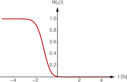
Figure 1: (Color) Ground-state depletion $W_{0}(t)$ at time $t$ of a nitrogen atom with the numerically-exact solution (solid-black lines) and the linearity theorem (II.2) (dashed-red lines).

In Fig. 1, I plot the numerically-exact solution of the rate equations for a nitrogen atom together with the result from the linearity theorem (II.2). Both curves are indistinguishable which is not surprising as the rate-equation for ground-state depletion (1) does not contain any decay terms.

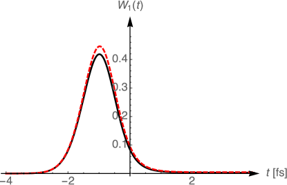
Figure 2: (Color) Single ionization $W_{1}(t)$ at time $t$ of a nitrogen atom. Line styles as in Fig. 1.

Single ionization is investigated in Fig. 2 and, again, a good agreement with the reference curve is found. However, this time, there is a decay term in the rate equations (III.1) which leads to a easily discernible deviation between both curves at the peak. The fact that the long-term behavior of both curves agrees so well can only be ascribed to the fact that further ionization of the atom leads to the observed decay and not Auger or radiative decay as they are not described by the linearity theorem (II.2).

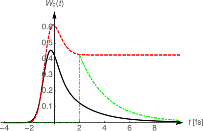
Figure 3: (Color) Double ionization $W_{2}(t)$ at time $t$ of a nitrogen atom with the numerically-exact solution (solid-black lines), the linearity theorem (II.2) (dashed-red lines), and the decay equation (20) (dotdashed-green lines).

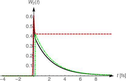
Figure 4: (Color) Double ionization $W_{2}(t)$ as in Fig. 3 but for an x-ray pulse with a FWHM duration of $200\,{\rm{as}}$.

The decay equations (20) are used in Fig. 3 and Fig. 4 for x-ray pulses with a FWHM duration of $2\,{\rm{fs}}$ and $200\,{\rm{as}}$, respectively, to examine double ionization. Thereby, I choose the time when the decay processes start $\mathfrak{T}$ to be the FWHM duration but the time $T$ at which the linearity theorem (II.2) is evaluated is chosen larger than $\mathfrak{T}$. Clearly, the curve from the decay equations in Fig. 3 shows a significant improvement over the result from the linearity theorem but does not approximate the numerically-exact solution acceptably. This changes dramatically if the FWHM pulse duration is decreased by an order of magnitude to $200\,{\rm{as}}$ in Fig. 4 where a good agreement is achieved. After the pulse is over the double ionization probability rises on the time scale of Auger decay of core holes of $6.7\,{\rm{fs}}$ Buth et al. (2012) which turns singly ionized nitrogen atoms into doubly ionized ones. Noteworthy is that this good agreement seen for double ionization does not remain so for charge states of N⁴⁺ and higher Sup . For them, to be accurately described by the decay equation, one needs to shorten the pulse duration even further in order to reduce the interplay between photoionization and decay processes. However, I need to stress that even assuming a $200\,{\rm{as}}$ pulse is stretching the validity of the rate-equation approximation too much. For such short pulses, coherence effects become important. Li et al. (2016) The upshot of the analysis of the decay equations (20) in this paragraph is that they are of limited use in the x-ray regime.

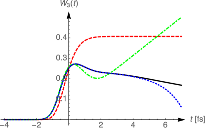
Figure 5: (Color) Triple ionization $W_{3}(t)$ at time $t$ of a nitrogen atom with the numerically-exact solution (solid-black lines), the linearity theorem (II.2) (dashed-red lines), and the successive approximation (37) in first (dash-dotted-green) and eighth order (dotted-blue).

Triple ionization of a nitrogen atom is displayed in Fig. 5 for the results from the linearity theorem, the successive approximation, and the numerically-exact solution. The linearity theorem produces a curve which only very crudely follows the behavior of the numerically-exact solution. Clearly, the absence of decay processes in the approximation leads to the overpopulation of the triple-ionization channels for $t>0$. Furthermore, after the pulse is over, the probability remains constant whereas the numerically-exact solution slopes downward due to decay processes. Taking decay into account in terms of the successive approximation (37) in first order leads to a good agreement up to $\approx 0.5\,{\rm{fs}}$. Afterwards the approximation quickly deteriorates. However, going to eighth order in the approximation of the Volterra integral equation improves the result dramatically such that it agrees with the numerically-exact solution up to $\approx 4.5\,{\rm{fs}}$. Still higher orders in the successive approximation are required to approximate the numerically-exact result beyond this time.

One needs to consider several terms in the successive approximation to reach converged solutions of the Volterra integral equation. As can be seen in Fig. 5, the first-order produces already good agreement for short times. However, to approximate the numerically-exact solution for longer times, higher orders are required. This can be understood by considering very short pulses for which the solution of the decay equation (20) is acceptable. Then the iteration of the Volterra integral equation needs to reproduce the terms of the series of the exponential function with the decay matrix in (20) up to sufficiently high order to obtain good agreement. The larger the time, the higher orders in the series need to be included.

V Conclusion

I carry out a formal analysis of multiphoton absorption which is called simultaneous, if it cannot be split into individual one- or few-photon absorptions but has to be described by the full expressions for the few-photon cross section. If a rate equation approximation turns out to be satisfactory, I can also distinguish linked multiphoton absorption—which are rendered nonlinear by the decay of intermediate states—and separable multiphoton absorption which depends only on the fluence the atom or molecule was subjected to—just like one-photon absorption. I turn to decay processes and analyze the situation under the assumption that the x-ray pulse is so short that one needs not consider decay in the course of it. Then the ensuing decay can be treated independently and an analytic expression is obtained for the probabilities to find the atom in specific states after the pulse is over. Finally, I solve the coupled rate equations that describe the joint process of x-ray absorption and decay. This is achieved by recasting the problem in terms of a Volterra integral equation of the second kind which is amenable to a solution by successive approximation. I apply the equations to a nitrogen atom in LCLS x rays which reveals that decay processes are crucial for an accurate description and the decay equation is acceptable only for very short pulses which makes it unattractive for applications in the x-ray regime. Yet for situations where the decay widths are considerably smaller than the case studied here, e.g., in the ultraviolet regime, the short-pulse approximation [Theorem 2] shall be much better and even Theorem 1 may find its use for approximating the quantum dynamics on short time scales. Clearly, if decay is absent, e.g., for the sequential absorption of outer valence electrons in ultraviolet light, Theorem 1 is the solution of the rate equations. In any case, the successive approximation provides a reliable and robust method to solve the rate equations. Already the first-order approximation to the solution of the Volterra equation is useful for small decay widths and limited duration, e.g., for computing x-ray diffraction of ultrashort pulses. Son, Young, and Santra (2011a); *Son:EH-11 However, higher orders need to be taken into account, if a longer time evolution is desired.

The presented research opens up rich perspectives for future work. The formulation of multiphoton absorption that has been devised here can be used in formal developments and practical applications. It provides a different viewpoint on the solution of the rate equations because the expression for the solution incorporates the underlying physics already in contrast to the conventional methods for numerically-solving systems of ordinary differential equations.

There are a two major challenges, however, involved in applying Theorems 1, 2, 4, and 5 in practical computations. First, the matrix exponentials need to be evaluated which requires careful numerical analysis. Golub and van Loan (1996); Moler and Van Loan (2003) Second, depending on the number of terms taken into account in Eq. (38), repeated numerical integrations are necessary. This is, of course, only the case, if Eq. (38) is applied; the mathematics of Volterra integral equations (33) and (39) is well researched and there are alternative methods available which may prove suitable for the problem at hand. Burton (1983); Linz (1985); Bakushinskii (originator) Both points need to be investigated further in order to turn this approach into a viable method in practice. Equation (39) has the advantage over Eq. (33) that the integral needs to be evaluated only for the duration of the x-ray pulse. Specifically, the systems of rate equations for heavy atoms become huge Fukuzawa et al. (2013); Ho et al. (2014) such that a complete numerical solution is rendered impracticable. Therefore, a Monte Carlo method is used in Refs. Fukuzawa et al., 2013; Ho et al., 2014 to solve the rate equations for which all atomic quantities, i.e., cross sections and decay widths are computed beforehand. Rudek et al. (2012); Son and Santra (2012); *Son:EM-15 For very heavy atoms and ionization of deep inner shells, even this is not enough as the computation of all involved atomic quantities becomes intractable. Hence the Monte Carlo approach is extended to also decide which quantities are to be calculated. Fukuzawa et al. (2013) Theorems 1, 2, 3, 4, and 5 provide a different perspective on the problem. Namely, the concept of Monte Carlo methods is replaced by matrix methods, i.e., the repeated solution of the rate equations involving random numbers is changed to an examination of matrix times vector products for sparse matrices. Golub and van Loan (1996) Decisions whether to compute certain atomic quantities need to be made based on their relevance to these products where suitable criteria need to be devised.

The rate equations in this work are restricted to non-resonant one-x-ray-absorption for simplicity and because it is the most important case for practical applications which rely frequently on x-ray diffraction. This limitation, however, can be lifted straightforwardly. One can include also REXMI terms, Rudek et al. (2012, 2013) if the rate-equation approximation remains valid for these cases. Delone and Krainov (2000) The solution of the rate equations with decay, Theorems 4 and 5, can be extended, e.g., to include simultaneous two-photon absorption Göppert-Mayer (1931); Rohringer and Santra (2007); Doumy et al. (2011) by augmenting the decay part in (19) by appropriate terms. The other way round is the case if there is no one-photon absorption, e.g., due to a too low photon energy. Then the analysis of Theorems 1, 2, 3, 4, and 5 can be done analogously starting with the lowest order of simultaneous multiphoton absorption instead. So far mostly configurations have been used in the literature to write down the rate equations. There is, however, no restriction that prevents one to use fine-structure-resolved states instead. This becomes relevant when heavier atoms are considered where relativistic effects are prominent. Rudek et al. (2012); Fukuzawa et al. (2013)

Appendix A Diagonalizability of a closed, lower triangular matrix

Lemma 2.

Given a real, lower triangular $K\times K$ matrix $A$ whose nonzero eigenvalues—the nonzero diagonal elements—are pairwise distinct; the eigenvalue 0 may occur multiple times. Furthermore, $A$ is a closed essentially nonnegative matrix. Then $A$ is diagonalizable and the eigenvectors corresponding to eigenvalues 0 are given by Cartesian eigenvectors $\hbox{\boldmath{$e$}\unboldmath}_{i}$ where $i\in\{1,\ldots,K\}$ and the value 1 in these vectors is at the row index $i$ of the eigenvalue 0 of $A$.

Proof.

As $A$ is closed (8) and essentially nonnegative, for $A_{ii}=0$ follows that $A_{ji}=0$ for all $j$, i.e., the entire column of $A$ is filled with zeros. Consequently, I have

$$\hbox{\boldmath{$A$}\unboldmath}\,\hbox{\boldmath{$e$}\unboldmath}_{i}=A_{ii}\,\hbox{\boldmath{$e$}\unboldmath}_{i}=\hbox{\boldmath{$0$}\unboldmath}\;.$$ (43)

Thus for all eigenvalues 0 of $A$ I have found eigenvectors, i.e., the algebraic multiplicity in the characteristic polynom due to eigenvalue 0 corresponds to its geometric multiplicity. All other eigenvalues are pairwise distinct. Hence the characteristic polynom contains only linear factors with respect to these eigenvalues. Thus $A$ is diagonalizable. Fischer (2014) ∎

References

- Walter (2000) W. Walter, Gewöhnliche Differentialgleichungen, 7th ed. (Springer-Verlag, Berlin, Heidelberg, 2000).
- Rohringer and Santra (2007) N. Rohringer and R. Santra, “X-ray nonlinear optical processes using a self-amplified spontaneous emission free-electron laser,” Phys. Rev. A 76, 033416 (2007).
- Son, Young, and Santra (2011a) S.-K. Son, L. Young, and R. Santra, “Impact of hollow-atom formation on coherent x-ray scattering at high intensity,” Phys. Rev. A 83, 033402 (2011a).
- Son, Young, and Santra (2011b) S.-K. Son, L. Young, and R. Santra, “Erratum: Impact of hollow-atom formation on coherent x-ray scattering at high intensity [Phys. Rev. A 83, 033402 (2011)],” Phys. Rev. A 83, 069906(E) (2011b).
- Buth et al. (2012) C. Buth, J.-C. Liu, M. H. Chen, J. P. Cryan, L. Fang, J. M. Glownia, M. Hoener, R. N. Coffee, and N. Berrah, “Ultrafast absorption of intense x rays by nitrogen molecules,” J. Chem. Phys. 136, 214310 (2012), arXiv:1201.1896 .
- Son and Santra (2012) S.-K. Son and R. Santra, “Monte Carlo calculation of ion, electron, and photon spectra of xenon atoms in x-ray free-electron laser pulses,” Phys. Rev. A 85, 063415 (2012).
- Son and Santra (2015) S.-K. Son and R. Santra, “Erratum: Monte Carlo calculation of ion, electron, and photon spectra of xenon atoms in x-ray free-electron laser pulses [Phys. Rev. A 85, 063415 (2012)],” Phys. Rev. A 92, 039906(E) (2015).
- Rudek et al. (2012) B. Rudek, S.-K. Son, L. Foucar, S. W. Epp, B. Erk, R. Hartmann, M. Adolph, R. Andritschke, A. Aquila, N. Berrah, C. Bostedt, J. Bozek, N. Coppola, F. Filsinger, H. Gorke, T. Gorkhover, H. Graafsma, L. Gumprecht, A. Hartmann, G. Hauser, S. Herrmann, H. Hirsemann, P. Holl, A. Homke, L. Journel, C. Kaiser, N. Kimmel, F. Krasniqi, K.-U. Kuhnel, M. Matysek, M. Messerschmidt, D. Miesner, T. Moller, R. Moshammer, K. Nagaya, B. Nilsson, G. Potdevin, D. Pietschner, C. Reich, D. Rupp, G. Schaller, I. Schlichting, C. Schmidt, F. Schopper, S. Schorb, C.-D. Schröter, J. Schulz, M. Simon, H. Soltau, L. Struder, K. Ueda, G. Weidenspointner, R. Santra, J. Ullrich, A. Rudenko, and D. Rolles, “Ultra-efficient ionization of heavy atoms by intense X-ray free-electron laser pulses,” Nat. Photon. 6, 858–865 (2012).
- Rudek et al. (2013) B. Rudek, D. Rolles, S.-K. Son, L. Foucar, B. Erk, S. Epp, R. Boll, D. Anielski, C. Bostedt, S. Schorb, R. Coffee, J. Bozek, S. Trippel, T. Marchenko, M. Simon, L. Christensen, S. De, S.-i. Wada, K. Ueda, I. Schlichting, R. Santra, J. Ullrich, and A. Rudenko, “Resonance-enhanced multiple ionization of krypton at an x-ray free-electron laser,” Phys. Rev. A 87, 023413 (2013).
- Fukuzawa et al. (2013) H. Fukuzawa, S.-K. Son, K. Motomura, S. Mondal, K. Nagaya, S. Wada, X.-J. Liu, R. Feifel, T. Tachibana, Y. Ito, M. Kimura, T. Sakai, K. Matsunami, H. Hayashita, J. Kajikawa, P. Johnsson, M. Siano, E. Kukk, B. Rudek, B. Erk, L. Foucar, E. Robert, C. Miron, K. Tono, Y. Inubushi, T. Hatsui, M. Yabashi, M. Yao, R. Santra, and K. Ueda, “Deep inner-shell multiphoton ionization by intense x-ray free-electron laser pulses,” Phys. Rev. Lett. 110, 173005 (2013).
- Ho et al. (2014) P. J. Ho, C. Bostedt, S. Schorb, and L. Young, “Theoretical tracking of resonance-enhanced multiple ionization pathways in x-ray free-electron laser pulses,” Phys. Rev. Lett. 113, 253001 (2014).
- Liu et al. (2016) J.-C. Liu, N. Berrah, L. S. Cederbaum, J. P. Cryan, J. M. Glownia, K. J. Schafer, and C. Buth, “Rate equations for nitrogen molecules in ultrashort and intense x-ray pulses,” J. Phys. B 49, 075602 (2016), arXiv:1508.05223 .
- Buth et al. (2017) C. Buth, R. Beerwerth, R. Obaid, N. Berrah, L. S. Cederbaum, and S. Fritzsche, “Neon in ultrashort and intense x rays from free-electron lasers,” submitted (2017), arXiv:1705.07521 .
- Arthur et al. (2002) J. Arthur, P. Anfinrud, P. Audebert, K. Bane, I. Ben-Zvi, V. Bharadwaj, R. Bionta, P. Bolton, M. Borland, P. H. Bucksbaum, R. C. Cauble, J. Clendenin, M. Cornacchia, G. Decker, P. Den Hartog, S. Dierker, D. Dowell, D. Dungan, P. Emma, I. Evans, G. Faigel, R. Falcone, W. M. Fawley, M. Ferrario, A. S. Fisher, R. R. Freeman, J. Frisch, J. Galayda, J.-C. Gauthier, S. Gierman, E. Gluskin, W. Graves, J. Hajdu, J. Hastings, K. Hodgson, Z. Huang, R. Humphry, P. Ilinski, D. Imre, C. Jacobsen, C.-C. Kao, K. R. Kase, K.-J. Kim, R. Kirby, J. Kirz, L. Klaisner, P. Krejcik, K. Kulander, O. L. Landen, R. W. Lee, C. Lewis, C. Limborg, E. I. Lindau, A. Lumpkin, G. Materlik, S. Mao, J. Miao, S. Mochrie, E. Moog, S. Milton, G. Mulhollan, K. Nelson, W. R. Nelson, R. Neutze, A. Ng, D. Nguyen, H.-D. Nuhn, D. T. Palmer, J. M. Paterson, C. Pellegrini, S. Reiche, M. Renner, D. Riley, C. V. Robinson, S. H. Rokni, S. J. Rose, J. Rosenzweig, R. Ruland, G. Ruocco, D. Saenz, S. Sasaki, D. Sayre, J. Schmerge, D. Schneider, C. Schroeder, L. Serafini, F. Sette, S. Sinha, D. van der Spoel, B. Stephenson, G. Stupakov, M. Sutton, A. Szöke, R. Tatchyn, A. Toor, E. Trakhtenberg, I. Vasserman, N. Vinokurov, X. J. Wang, D. Waltz, J. S. Wark, E. Weckert, Wilson-Squire Group, H. Winick, M. Woodley, A. Wootton, M. Wulff, M. Xie, R. Yotam, L. Young, and A. Zewail, “Linac Coherent Light Source (LCLS): Conceptual Design Report,” Tech. Rep. SLAC-R-593, UC-414 (Stanford Linear Accelerator Center (SLAC), Menlo Park, California, USA, 2002).
- Emma et al. (2010) P. Emma, R. Akre, J. Arthur, R. Bionta, C. Bostedt, J. Bozek, A. Brachmann, P. Bucksbaum, R. Coffee, F.-J. Decker, Y. Ding, D. Dowell, S. Edstrom, J. Fisher, A. Frisch, S. Gilevich, J. Hastings, G. Hays, P. Hering, Z. Huang, R. Iverson, H. Loos, M. Messerschmidt, A. Miahnahri, S. Moeller, H.-D. Nuhn, G. Pile, D. Ratner, J. Rzepiela, D. Schultz, T. Smith, P. Stefan, H. Tompkins, J. Turner, J. Welch, W. White, J. Wu, G. Yocky, and J. Galayda, “First lasing and operation of an ångstrom-wavelength free-electron laser,” Nature Photon. 4, 641–647 (2010).
- Ishikawa et al. (2012) T. Ishikawa, H. Aoyagi, T. Asaka, Y. Asano, N. Azumi, T. Bizen, H. Ego, K. Fukami, T. Fukui, Y. Furukawa, S. Goto, H. Hanaki, T. Hara, T. Hasegawa, T. Hatsui, A. Higashiya, T. Hirono, N. Hosoda, M. Ishii, T. Inagaki, Y. Inubushi, T. Itoga, Y. Joti, M. Kago, T. Kameshima, H. Kimura, Y. Kirihara, A. Kiyomichi, T. Kobayashi, C. Kondo, T. Kudo, H. Maesaka, X. M. Marechal, T. Masuda, S. Matsubara, T. Matsumoto, T. Matsushita, S. Matsui, M. Nagasono, N. Nariyama, H. Ohashi, T. Ohata, T. Ohshima, S. Ono, Y. Otake, C. Saji, T. Sakurai, T. Sato, K. Sawada, T. Seike, K. Shirasawa, T. Sugimoto, S. Suzuki, S. Takahashi, H. Takebe, K. Takeshita, K. Tamasaku, H. Tanaka, R. Tanaka, T. Tanaka, T. Togashi, K. Togawa, A. Tokuhisa, H. Tomizawa, K. Tono, S. Wu, M. Yabashi, M. Yamaga, A. Yamashita, K. Yanagida, C. Zhang, T. Shintake, H. Kitamura, and N. Kumagai, “A compact X-ray free-electron laser emitting in the sub-ångstrom region,” Nat. Photon. 6, 540–544 (2012).
- Ganter (2012) R. Ganter, ed., SwissFEL Conceptual Design Report, PSI Bericht Nr. 10-04 (Paul Scherrer Institut (PSI), Villigen, Switzerland, 2012) http://www.psi.ch/swissfel/CurrentSwissFELPublicationsEN/SwissFEL_CDR_V20_23.04.12_small.pdf.
- Altarelli et al. (2006) M. Altarelli, R. Brinkmann, M. Chergui, W. Decking, B. Dobson, S. Düsterer, G. Grübel, W. Graeff, H. Graafsma, J. Hajdu, J. Marangos, J. Pflüger, H. Redlin, D. Riley, I. Robinson, J. Rossbach, A. Schwarz, K. Tiedtke, T. Tschentscher, I. Vartaniants, H. Wabnitz, H. Weise, R. Wichmann, K. Witte, A. Wolf, M. Wulff, and M. Yurkov, eds., XFEL: The European X-Ray Free-Electron Laser - Technical Design Report, DESY 2006-097 (DESY XFEL Project Group, Deutsches Elektronen-Synchrotron (DESY), Notkestraße 85, 22607 Hamburg, Germany, 2006).
- L’Huillier et al. (1983a) A. L’Huillier, L. A. Lompre, G. Mainfray, and C. Manus, “Multiply charged ions induced by multiphoton absorption processes in rare-gas atoms at ,” J. Phys. B 16, 1363–1381 (1983a).
- L’Huillier et al. (1983b) A. L’Huillier, L. A. Lompre, G. Mainfray, and C. Manus, “Multiply charged ions induced by multiphoton absorption in rare gases at ,” Phys. Rev. A 27, 2503–2512 (1983b).
- L’Huillier et al. (1983c) A. L’Huillier, L. A. Lompre, G. Mainfray, and C. Manus, “Laser pulse duration effects in Xe2+ ions induced by multiphoton absorption at ,” J. Phys. France 44, 1247–1255 (1983c).
- Crance and Aymar (1985) M. Crance and M. Aymar, “Competition between direct process and stepwise process in multiphoton stripping of atoms. A model calculation in helium,” J. Phys. France 46, 1887–1896 (1985).
- Lambropoulos and Tang (1987) P. Lambropoulos and X. Tang, “Multiple excitation and ionization of atoms by strong lasers,” J. Opt. Soc. Am. B 4, 821–832 (1987).
- Delone and Krainov (2000) N. B. Delone and V. P. Krainov, Multiphoton Processes in Atoms, 2nd ed., edited by P. Lambropoulos, Atoms and Plasmas, Vol. 13 (Springer, Berlin, 2000).
- Hoener et al. (2010) M. Hoener, L. Fang, O. Kornilov, O. Gessner, S. T. Pratt, M. Gühr, E. P. Kanter, C. Blaga, C. Bostedt, J. D. Bozek, P. H. Bucksbaum, C. Buth, M. Chen, R. Coffee, J. Cryan, L. DiMauro, M. Glownia, E. Hosler, E. Kukk, S. R. Leone, B. McFarland, M. Messerschmidt, B. Murphy, V. Petrovic, D. Rolles, and N. Berrah, “Ultraintense x-ray induced ionization, dissociation, and frustrated absorption in molecular nitrogen,” Phys. Rev. Lett. 104, 253002 (2010).
- Young et al. (2010) L. Young, E. P. Kanter, B. Krässig, Y. Li, A. M. March, S. T. Pratt, R. Santra, S. H. Southworth, N. Rohringer, L. F. DiMauro, G. Doumy, C. A. Roedig, N. Berrah, L. Fang, M. Hoener, P. H. Bucksbaum, J. P. Cryan, S. Ghimire, J. M. Glownia, D. A. Reis, J. D. Bozek, C. Bostedt, and M. Messerschmidt, “Femtosecond electronic response of atoms to ultra-intense x-rays,” Nature 466, 56–61 (2010).
- Obaid et al. (2017) R. Obaid, C. Buth, G. Dakovski, R. Beerwerth, M. Holmes, J. Aldrich, M.-F. Lin, M. Minitti, T. Osipov, W. Schlotter, L. S. Cederbaum, S. Fritzsche, and N. Berrah, “LCLS in – photon out: fluorescence measurement of neon using soft x-rays,” submitted (2017), arXiv:1708.01283 .
- Xiang et al. (2012) W. Xiang, C. Gao, Y. Fu, J. Zeng, and J. Yuan, “Inner-shell resonant absorption effects on evolution dynamics of the charge state distribution in a neon atom interacting with ultraintense x-ray pulses,” Phys. Rev. A 86, 061401(R) (2012).
- Rohringer and Santra (2008a) N. Rohringer and R. Santra, “Resonant Auger effect at high x-ray intensity,” Phys. Rev. A 77, 053404 (2008a).
- Rohringer and Santra (2008b) N. Rohringer and R. Santra, “Publisher’s Note: Resonant Auger effect at high x-ray intensity [Phys. Rev. A 77, 053404 (2008)],” Phys. Rev. A 77, 059903(E) (2008b).
- Kanter et al. (2011) E. P. Kanter, B. Krässig, Y. Li, A. M. March, P. Ho, N. Rohringer, R. Santra, S. H. Southworth, L. F. DiMauro, G. Doumy, C. A. Roedig, N. Berrah, L. Fang, M. Hoener, P. H. Bucksbaum, S. Ghimire, D. A. Reis, J. D. Bozek, C. Bostedt, M. Messerschmidt, and L. Young, “Unveiling and driving hidden resonances with high-fluence, high-intensity x-ray pulses,” Phys. Rev. Lett. 107, 233001 (2011).
- Cavaletto et al. (2012) S. M. Cavaletto, C. Buth, Z. Harman, E. P. Kanter, S. H. Southworth, L. Young, and C. H. Keitel, “Resonance fluorescence in ultrafast and intense x-ray free electron laser pulses,” Phys. Rev. A 86, 033402 (2012), arXiv:1205.4918 .
- Cavaletto et al. (2013) S. M. Cavaletto, Z. Harman, C. Buth, and C. H. Keitel, “X-ray frequency combs from optically controlled resonance fluorescence,” Phys. Rev. A 88, 063402 (2013), arXiv:1302.3141 .
- Adams et al. (2013) B. W. Adams, C. Buth, S. M. Cavaletto, J. Evers, Z. Harman, C. H. Keitel, A. Pálffy, A. Picón, R. Röhlsberger, Y. Rostovtsev, and K. Tamasaku, “X-ray quantum optics,” J. Mod. Opt. 60, 2–21 (2013).
- Cavaletto et al. (2014) S. M. Cavaletto, Z. Harman, C. Ott, C. Buth, T. Pfeifer, and C. H. Keitel, “Broadband high-resolution x-ray frequency combs,” Nature Photon. 8, 520–523 (2014), arXiv:1402.6652 .
- Li et al. (2016) Y. Li, C. Gao, W. Dong, J. Zeng, Z. Zhao, and J. Yuan, “Coherence and resonance effects in the ultra-intense laser-induced ultrafast response of complex atoms,” Sci. Rep. 6, 18529 (2016).
- Als-Nielsen and McMorrow (2001) J. Als-Nielsen and D. McMorrow, Elements of Modern X-Ray Physics (John Wiley & Sons, New York, 2001).
- Makris, Lambropoulos, and Mihelič (2009) M. G. Makris, P. Lambropoulos, and A. Mihelič, “Theory of multiphoton multielectron ionization of xenon under strong 93-eV radiation,” Phys. Rev. Lett. 102, 033002 (2009).
- Doumy et al. (2011) G. Doumy, C. Roedig, S.-K. Son, C. I. Blaga, A. D. DiChiara, R. Santra, N. Berrah, C. Bostedt, J. D. Bozek, P. H. Bucksbaum, J. P. Cryan, L. Fang, S. Ghimire, J. M. Glownia, M. Hoener, E. P. Kanter, B. Krässig, M. Kuebel, M. Messerschmidt, G. G. Paulus, D. A. Reis, N. Rohringer, L. Young, P. Agostini, and L. F. DiMauro, “Nonlinear atomic response to intense ultrashort x rays,” Phys. Rev. Lett. 106, 083002 (2011).
- Tamasaku et al. (2014) K. Tamasaku, E. Shigemasa, Y. Inubushi, T. Katayama, K. Sawada, H. Yumoto, H. Ohashi, H. Mimura, M. Yabashi, K. Yamauchi, and T. Ishikawa, “X-ray two-photon absorption competing against single and sequential multiphoton processes,” Nat. Photon. 8, 313–316 (2014).
- Neutze et al. (2000) R. Neutze, R. Wouts, D. van der Spoel, E. Weckert, and J. Hajdu, “Potential for biomolecular imaging with femtosecond x-ray pulses,” Nature 406, 752–757 (2000).
- Cryan et al. (2010) J. P. Cryan, J. M. Glownia, J. Andreasson, A. Belkacem, N. Berrah, C. I. Blaga, C. Bostedt, J. Bozek, C. Buth, L. F. DiMauro, L. Fang, O. Gessner, M. Guehr, J. Hajdu, M. P. Hertlein, M. Hoener, O. Kornilov, J. P. Marangos, A. M. March, B. K. McFarland, H. Merdji, V. S. Petrović, C. Raman, D. Ray, D. Reis, F. Tarantelli, M. Trigo, J. L. White, W. White, L. Young, P. H. Bucksbaum, and R. N. Coffee, “Auger electron angular distribution of double core hole states in the molecular reference frame,” Phys. Rev. Lett. 105, 083004 (2010).
- Fang et al. (2010) L. Fang, M. Hoener, O. Gessner, F. Tarantelli, S. T. Pratt, O. Kornilov, C. Buth, M. Gühr, E. P. Kanter, C. Bostedt, J. D. Bozek, P. H. Bucksbaum, M. Chen, R. Coffee, J. Cryan, M. Glownia, E. Kukk, S. R. Leone, and N. Berrah, “Double core hole production in N2: Beating the Auger clock,” Phys. Rev. Lett. 105, 083005 (2010), arXiv:1303.1429 .
- Fang et al. (2012) L. Fang, T. Osipov, B. Murphy, F. Tarantelli, E. Kukk, J. Cryan, P. H. Bucksbaum, R. N. Coffee, M. Chen, C. Buth, and N. Berrah, “Multiphoton ionization as a clock to reveal molecular dynamics with intense short x-ray free electron laser pulses,” Phys. Rev. Lett. 109, 263001 (2012), arXiv:1301.6459 .
- Note (1) The essence of the linearity theorem of multiphoton absorption has already been stated in the third paragraph in the left column on page 2 of Ref. \rev@citealpnumButh:UA-12.
- Göppert-Mayer (1931) M. Göppert-Mayer, “Über Elementarakte mit zwei Quantensprüngen,” Ann. Phys. (Leipzig) 17, 273–294 (1931).
- Hartree (1928) D. R. Hartree, “The wave mechanics of an atom with a non-coulomb central field. Part I. Theory and methods,” Proc. Camb. Phil. Soc. 24, 89–110 (1928).
- Szabo and Ostlund (1989) A. Szabo and N. S. Ostlund, Modern Quantum Chemistry: Introduction to Advanced Electronic Structure Theory, 1st, revised ed. (McGraw-Hill, New York, 1989).
- (49) See the Supplementary Data for a Mathematica Mat (2016) file with all computations presented in this work.
- Mat (2016) Mathematica 11, Wolfram Research, Inc., 100 Trade Center Drive, Champaign, Illinois 61820-7237, USA (2016).
- Note (2) For conceptual ease, I restrict myself here in considering the final state to be electron-bare which, however, is not necessarily required. Instead the single final state may also be a configuration which still has electrons in deep lying shells which is energetically to high in energy such that it cannot be ionized by the photons with the given energy and is not amenable to REXMI. Rudek et al. (2012, 2013).
- Note (3) A fixed photon energy is assumed which needs to be high enough such that all electrons can be ionized; the dependence of the quantities on the photon energy is omitted throughout. If the x-ray photon energy is lower than the energy that is necessary to strip the system of all electrons, then the total absorption cross section of this last configuration—I assume that there is a single last configuration—is zero, although there are still electrons in lower lying shells. Increasing the x-ray photon energy renders the total absorption cross section nonzero. Please see figure 2 in Buth et al. (2012) and its explanation. Only cationic configurations are included without regarding shake-off or shake-up processes and other multielectron effects such as double Auger decay.
- Pauli (1928) W. Pauli, “Über das H-Theorem vom Anwachsen der Entropie vom Standpunkt der neueren Quantenmechanik,” in Probleme der modernen Physik, edited by P. Debye (S. Hirzel, Leipzig, 1928) pp. 30–45, Arnold Sommerfeld zum 60. Geburtstag, gewidmet von seinen Schülern.
- Louisell (1990) W. H. Louisell, Quantum Statistical Properties of Radiation, Wiley Classics Library (John Wiley & Sons, New York, 1990).
- Buth (2017) C. Buth, “Dissociating diatomic molecules in ultrafast and intense light,” submitted (2017), arXiv:1708.09615 .
- Krengel (2005) U. Krengel, Einführung in die Wahrscheinlichkeitstheorie und Statistik, 8th ed., vieweg studium; Aufbaukurs Mathematik, Vol. 59 (Vieweg+Teubner Verlag, Wiesbaden, 2005).
- Kuptsov (originator) L. P. Kuptsov (originator), “Kronecker symbol,” Encyclopedia of Mathematics (2016), http://www.encyclopediaofmath.org/index.php?title=Kronecker_symbol&oldid=37525. Accessed 03 April 2017.
- Giorgio and Zuccotti (2015) G. Giorgio and C. Zuccotti, “Metzlerian and generalized Metzlerian matrices: some properties and economic applications,” J. Math. Res. 7, 42–55 (2015).
- Komlenko (originator) Y. V. Komlenko (originator), “Fundamental matrix,” Encyclopedia of Mathematics (2011), http://www.encyclopediaofmath.org/index.php?title=Fundamental_matrix&oldid=14038. Accessed 21 March 2017.
- Sorokin et al. (2007) A. A. Sorokin, S. V. Bobashev, T. Feigl, K. Tiedtke, H. Wabnitz, and M. Richter, “Photoelectric effect at ultrahigh intensities,” Phys. Rev. Lett. 99, 213002 (2007).
- Fischer (2014) G. Fischer, Lineare Algebra, 18th ed., Grundkurs Mathematik (Springer Spektrum, Wiesbaden, 2014).
- Baake and Schlägel (2011) M. Baake and U. Schlägel, “The Peano-Baker series,” Proc. Steklov Inst. Math. 275, 155–159 (2011), arXiv:1011.1775 .
- Burton (1983) T. A. Burton, Volterra Integral and Differential Equations, Mathematics in science and engineering No. 167 (Academic Press, New York, 1983).
- Linz (1985) P. Linz, Analytical and Numerical Methods for Volterra Equations, SIAM studies in applied mathematics No. 7 (Society for Industrial and Applied Mathematics, Philadelphia, 1985).
- Bakushinskii (originator) A. B. Bakushinskii (originator), “Volterra equation,” Encyclopedia of Mathematics (2011), http://www.encyclopediaofmath.org/index.php?title=Volterra_equation&oldid=15168. Accessed 09 November 2016.
- Khvedelidze (originator) B. V. Khvedelidze (originator), “Sequential approximation, method of,” Encyclopedia of Mathematics (2011), http://www.encyclopediaofmath.org/index.php?title=Sequential_approximation,_method_of&oldid=14953. Accessed 09 November 2016.
- Fetter and Walecka (1971) A. L. Fetter and J. D. Walecka, Quantum Theory of Many-Particle Systems, International Series in Pure and Applied Physics, edited by Leonard I. Schiff (McGraw-Hill, New York, 1971).
- Golub and van Loan (1996) G. H. Golub and C. F. van Loan, Matrix Computations, 3rd ed. (Johns Hopkins University Press, Baltimore, 1996).
- Moler and Van Loan (2003) C. Moler and C. Van Loan, “Nineteen dubious ways to compute the exponential of a matrix, twenty-five years later,” SIAM Rev. 45, 3–49 (2003).