Electromagnetic instability and Schwinger effect in the Witten-Sakai-Sugimoto model with D0-D4 background

Wenhe Cai ,3,4,5)   Kang-le Li ,4)   Si-wen Li ,1,2,4) whcai@shu.edu.cnlkl96@mail.ustc.edu.cnsiwenli@dlmu.edu.cn
Abstract

Using the Witten-Sakai-Sugimoto model in the D0-D4 background, we holographically compute the vacuum decay rate of the Schwinger effect in this model. Our calculation contains the influence of the D0-brane density which could be identified as the $\theta$ angle or chiral potential in QCD. Under the strong electromagnetic fields, the instability appears due to the creation of quark-antiquark pairs and the associated decay rate can be obtained by evaluating the imaginary part of the effective Euler-Heisenberg action which is identified as the action of the probe brane with a constant electromagnetic field. In the bubble D0-D4 configuration, we find the decay rate decreases when the $\theta$ angle increases since the vacuum becomes heavier in the present of the glue condensate in this system. And the decay rate matches to the result in the black D0-D4 configuration at zero temperature limit according to our calculations. In this sense, the Hawking-Page transition of this model could be consistently interpreted as the confined/deconfined phase transition. Additionally there is another instability from the D0-brane itself in this system and we suggest that this instability reflects to the vacuum decay triggered by the $\theta$ angle as it is known in the $\theta$-dependent QCD.

1Department of Physics, Dalian Maritime University, Dalian 116033, China

2Department of Physics, Center for Field Theory and Particle Physics, Fudan University, Shanghai 200433, China

3Department of Physics, Shanghai University, Shanghai 200444, China

4Department of Modern Physics, University of Science and Technology of China, Hefei 230026, Anhui, China

5Interdisciplinary Center for Theoretical Study, University of Science and Technology of China, Hefei 230026, Anhui, China

1 Introduction

Recent years, there have been many advances in the researches on the strong electromagnetic field, especially in heavy-ion collision since it is expected that an extremely strong magnetic field is generated by the collision of the charged particles. In particular, the Schwinger effect should be one of the most interesting phenomena in the heavy-ion collision, because the pair creation of charged particles from the vacuum occurs under such an externally strong electromagnetic field. In the Schwinger effect, the creation rate of a pair of charged particles could be obtained by evaluating the imaginary part of Euler-Heisenberg Lagrangian [1, 2]. However, the result implies the Schwinger effect is a non-perturbative effect which shows up only under the strong electromagnetic field.

Although it is still challenging to evaluate the Schwinger effect under the electromagnetic field, the framework of gauge/gravity duality or AdS/CFT provides a powerful tool on studying the strongly coupled quantum field theories [3, 4, 5]. It has been recognized that a (d+2)-dimensional classical gravity theory could correspond to a (d+1)-dimensional gauge theory as a weak/strong duality. So with this framework, various applications of studying the Schwinger effect holographically have been presented [6, 7, 8, 9, 10, 11, 12, 13, 14, 15]. Particularly, in some top-down holographic approaches e.g. the D3/D7 approach, since the dynamics of the flavors is described by the action of the probe flavor brane, the associated decay rate to the Schwinger effect could be evaluated by using the flavored action. Hence it implies this action could be identified as the holographic Euler-Heisenberg action and the creation rate of flavored quark-antiquark pairs (i.e. the vacuum decay rate) can be computed by the imaginary part of this action [13, 14, 15]. While this is a different method, it allows us to quantitatively explore the electromagnetic instability and Schwinger effect in holography.

On the other hand, the $\theta$-dependence in QCD or Yang-Mills theory is also interesting [16, 17]. The $\theta$-dependent gauge theories contain a Chern-Simons term as a topological term additional to the action and the coupling of the Chern-Simons term is named as the $\theta$ angle (as the following form),

$$S=\frac{1}{2g_{YM}^{2}}\int\mathrm{Tr}F\wedge^{*}F-i\frac{\theta}{16\pi^{2}}\int\mathrm{Tr}F\wedge F,$$ (1)

where $g_{YM}$ is the Yang-Mills coupling constant and $F$ is the gauge field strength. While the experimental value of $\theta$ is small, the Chern-Simons term leads to many observable phenomena such as chiral anomaly [18], chiral magnetic effect [19], deconfinement transition [20, 21] and effects of gluon condensate. Accordingly, to investigate the Schwinger effect with $\theta$-dependence in QCD would be significant since the creation rate of quark-antiquark pairs is affected by the $\theta$ angle. So in this paper, we are motivated to study the electromagnetic instability and the Schwinger effect with such a topological term in holography.

In the gauge/gravity duality, the $\theta$-dependence could be introduced as the D-brane with D-instanton configuration in the string theory [22, 23]. Thus we use the Witten-Sakai-Sugimoto model in the D0-D4 background (i.e. the D0-D4/D8 system) where D0-brane could be the D-instanton in our investigation since this system is holographically dual to QCD with a Chern-Simons term [24, 25, 26] (See more details and applications in [27, 28, 29, 30]). In this model, the background geometry is produced by $N_{c}$ coincident D4-branes wrapped on a cycle with $N_{0}$ smeared D0-branes inside their worldvolume. The supersymmetry is broken down by imposing the anti-periodic boundary condition on fermions. In the presence of the D0-branes, the effective action of the D4-branes takes the following form,

$\displaystyle S_{D_{4}}$ $\displaystyle=$ $\displaystyle-\mu_{4}\mathrm{Tr}\int d^{4}xdx^{4}e^{-\phi}\sqrt{-\det\left(\mathcal{G}+\mathcal{F}\right)}$ (2)
$\displaystyle+\mu_{4}\int C_{5}+\frac{1}{2}\mu_{4}\int C_{1}\wedge\mathcal{F}\wedge\mathcal{F},$

where $\mu_{4}=\left(2\pi\right)^{-4}l_{s}^{-5}$, $l_{s}$ is the length of the string, $\mathcal{G}$ is the induced metric on the worldvolume. $\mathcal{F}=2\pi\alpha^{\prime}F$ is the gauge field strength on the D4-brane. $C_{5},\ C_{1}$ is the Romand-Romand 5- and 1- form respectively. We have used $x^{4}$ to represent the wrapped direction which is periodic. The first term in (2) is the Dirac-Born-Infeld (DBI) action and the Yang-Mills action comes from its leading-order expansion respected to $\mathcal{F}$. In the bubble D0-D4 solution, we have $C_{1}\sim\theta dx^{4}$ [25], thus D0-branes are actually D-instantons and the last term in (2) could be integrated as,

$$\int_{S^{1}}C_{1}\sim\theta,\ \ \ \ \int_{S^{1}\times\mathrm{R}^{4}}C_{1}\wedge\mathcal{F}\wedge\mathcal{F}\sim\theta\int_{\mathrm{R}^{4}}\mathcal{F}\wedge\mathcal{F}.$$ (3)

Therefore the number density of D0-branes (D0 charge) is related to the $\theta$ angle and we could finally obtain the Yang-Mills plus Chern-Simons action (1) from (2) and (3) as the low-energy theory of the bubble D0-D4 system. As the analysis of the D4/D8 model (the original Witten-Sakai-Sugimoto model) [31, 32, 33, 34, 35], the bubble D0-D4 corresponds to the confinement phase of the dual field theory while the black D0-D4 corresponds to the deconfinement phase111In [36], an alternative solution for the deconfinement phase has been proposed .. However in the black D0-D4 configuration, the physical interpretation of D0-brane is less clear since D0-brane is not D-instanton. Nevertheless, we might identify the D0 charge as the chiral potential in the black D0-D4 configuration according to the phenomenal evidences presented in [37, 38, 39]. Besides, the flavors can be introduced by a stack of $N_{f}$ D8 and anti-D8 branes ($\mathrm{D}8/\overline{\mathrm{D}8}$-branes) as probes into the D0-D4 background. Hence the chirally symmetric or broken phase of the dual field theory is represented by the various configurations of $\mathrm{D}8/\overline{\mathrm{D}8}$-branes in the bubble or black D0-D4 background.

In this paper, we will focus on the derivation of the effective Euler-Heisenberg Lagrangian first, then we could explore the electromagnetic instability and evaluate the creation rate of quark-antiquark pairs in the vacuum. The paper is organized as follows, in section 2, we review the Witten-Sakai-Sugimoto model in the D0-D4 background with more details. In section 3, we derive the the effective Euler-Heisenberg Lagrangian from the probe $\mathrm{D}8/\overline{\mathrm{D}8}$-branes action in the bubble and black D0-D4 background respectively. In section 4, we evaluate the creation rate of quark-antiquark pairs in the vacuum. In the black D0-D4 background, we find the creation rate is finite at zero temperature limit which qualitatively coincides with the results from the bubble D0-D4 background. In this sense, we suggest that the Hawking-Page transition of this model is suitable to be identified as the confined/deconfined phase transition. And our numerical calculation shows the creation rate decreases when the D0 density ($\theta$ angle) increases in the bubble D0-D4 case. This may be interpreted as that the vacuum becomes heavier due to the gluon condensate described by this model in terms of quantum field theory. The final section is the summary and discussion.

2 Review of the Witten-Sakai-Sugimoto model in the D0-D4 background

In this section, let us briefly review the Witten-Sakai-Sugimoto model in the D0-D4 background (i.e. the D0-D4/D8 system). In string frame, the background geometry described by the bubble solution of $N_{c}$ D4 branes with smeared $N_{0}$ D0 charges. The near horizon metric reads in type IIA supergravity [25, 26, 27],

$\displaystyle ds^{2}=$ $\displaystyle\left(\frac{U}{R}\right)^{3/2}\left[H_{0}^{1/2}\eta_{\mu\nu}dX^{\mu}dX^{\nu}+H_{0}^{-1/2}f\left(U\right)\left(dX^{4}\right)^{2}\right]$
$\displaystyle+H_{0}^{1/2}\left(\frac{R}{U}\right)^{3/2}\left[\frac{dU^{2}}{f\left(U\right)}+U^{2}d\Omega_{4}^{2}\right].$ (4)

The D0-branes are smeared in the $X^{i},\ i=1,2,3$ and $X^{4}$. $N_{c}$ represents the number of colors. The dilaton, the field strength of the Ramond-Ramond field, the function $f(U),\ H_{0}\left(U\right)$ and the radius $R$ of the bulk are given as follows,

$\displaystyle e^{\phi}=g_{s}\left(\frac{U}{R}\right)^{3/4}H_{0}^{3/4},\ \ F_{2}=\frac{1}{\sqrt{2!}}\frac{\mathcal{A}}{U^{4}}\frac{1}{H_{0}^{2}}dU\wedge dX^{4},\ \ F_{4}=\frac{1}{\sqrt{4!}}\mathcal{B}\epsilon_{4},\ \ f(U)\equiv 1-\frac{U_{KK}^{3}}{U^{3}},$
$\displaystyle R^{3}\equiv\pi g_{s}N_{c}l_{s}^{3},\ \ H_{0}=1+\frac{U_{Q_{0}}^{3}}{U^{3}},\ \ \mathcal{A}=\frac{\left(2\pi l_{s}\right)^{7}g_{s}N_{0}}{\omega_{4}V_{4}},\ \ \mathcal{B}=\frac{\left(2\pi l_{s}\right)^{3}g_{s}N_{c}}{\omega_{4}}.$ (5)

where $\mathcal{A},\ \mathcal{B}$ are two integration constants given as,

$$\mathcal{A}=3\sqrt{U_{Q_{0}}^{3}\left(U_{Q_{0}}^{3}+U_{KK}^{3}\right)},\ \ \mathcal{B}=3\sqrt{U_{Q_{4}}^{3}\left(U_{Q_{4}}^{3}+U_{KK}^{3}\right)}.$$ (6)

We use $U_{KK}$, $g_{s}$, $l_{s}$, $V_{4}$ and $\epsilon_{4}$ to represent the coordinate radius of the bottom of the bubble, the string coupling, the string length, the volume of the unit four sphere $S^{4}$ and the volume form of the $S^{4}$ respectively. $\alpha^{\prime}$ is defined as $l_{s}^{2}=\alpha^{\prime}$. The coordinate $U$ is the holographic radial direction, and $U\rightarrow\infty$ corresponds to the boundary of the bulk. Therefore coordinate $U$ takes the values in the region $U_{KK}\leq U\leq\infty$. In order to avoid a possible singularity at $U=U_{KK}$, the coordinate $U$ satisfies the following periodic boundary condition [24],

$$X^{4}\sim X^{4}+\delta X^{4},\ \ \delta X^{4}=\frac{4\pi}{3}\frac{R^{3/2}}{U_{KK}^{1/2}}H_{0}^{1/2}\left(U_{KK}\right)=2\pi R.$$ (7)

So the Kaluza-Klein mass parameter is obtained,

$$M_{KK}=\frac{2\pi}{\delta X^{4}}=\frac{3U_{KK}^{1/2}}{2R^{3/2}}H_{0}^{-1/2}\left(U_{KK}\right).$$ (8)

The gauge coupling $g_{YM}$ at the cut-off scale $M_{KK}$ in the 4-dimensional Yang-Mills theory is derived as $g_{YM}^{2}=(2\pi)^{2}g_{s}l_{s}/\delta X^{4}$ from the 5-dimensional D4-brane compactified on $S^{1}$. Thus, according to the gauge/gravity duality and AdS/CFT dictionary, the relationship between the parameters $R,U_{KK},g_{s},U_{Q_{0}}$ (in the gravity side) and the parameters $M_{KK},\lambda,N_{c},H_{0}(U_{KK})$ expressed in QCD is given as,

$$R^{3}=\frac{1}{2}\frac{\lambda l_{s}^{2}}{M_{KK}},\ \ U_{KK}=\frac{2}{9}\lambda M_{KK}l_{s}^{2}H_{KK},\ \ g_{s}=\frac{1}{2\pi}\frac{\lambda}{M_{KK}N_{c}l_{s}},$$ (9)

where $H_{KK}\equiv H_{0}\left(U_{KK}\right)$ and $\lambda\equiv g_{YM}^{2}N_{c}$ is the 4-dimensional ’t Hooft coupling. Since one of the spatial coordinates, denoted by $X^{4}$, is compactified on $S^{1}$, the fermions (and other irrelevant fields) would be massive by imposing the anti-periodic boundary condition on the cycle $S^{1}$, thus they are decoupled from the low-energy theory. Accordingly, the effective theory consists of the Yang-Mills fields only.

There is an alternatively allowed solution for the D0-D4/D8 system which is the black brane solution. This solution could be obtained by interchanging the coordinate $X^{4}$ and $X^{0}$ in (4). So the metric reads [30, 39],

$\displaystyle ds_{D4}^{2}=$ $\displaystyle\left(\frac{U}{R}\right)^{3/2}\left[-H_{0}^{-1/2}f_{T}\left(U\right)dt^{2}+H_{0}^{1/2}\delta_{ij}dX^{i}dX^{j}+H_{0}^{1/2}\left(dX^{4}\right)^{2}\right]$
$\displaystyle+H_{0}^{1/2}\left(\frac{R}{U}\right)^{3/2}\left[\frac{dU^{2}}{f_{T}\left(U\right)}+U^{2}d\Omega_{4}^{2}\right].$ (10)

where the function $f_{T}\left(U\right)$ is given as222In the black D0-D4 solution, we replace $U_{KK}$ by $U_{T}$ in the solution.,

$$f_{T}\left(U\right)=1-\frac{U_{T}^{3}}{U^{3}}.$$ (11)

The solution for the other fields in the black D0-D4 background could also be obtained after interchanging $X^{4}$ and $X^{0}$ in (5). The metric (10) describes a horizon at $U=U_{T}$, thus it corresponds to a quantum field theory at finite temperature.

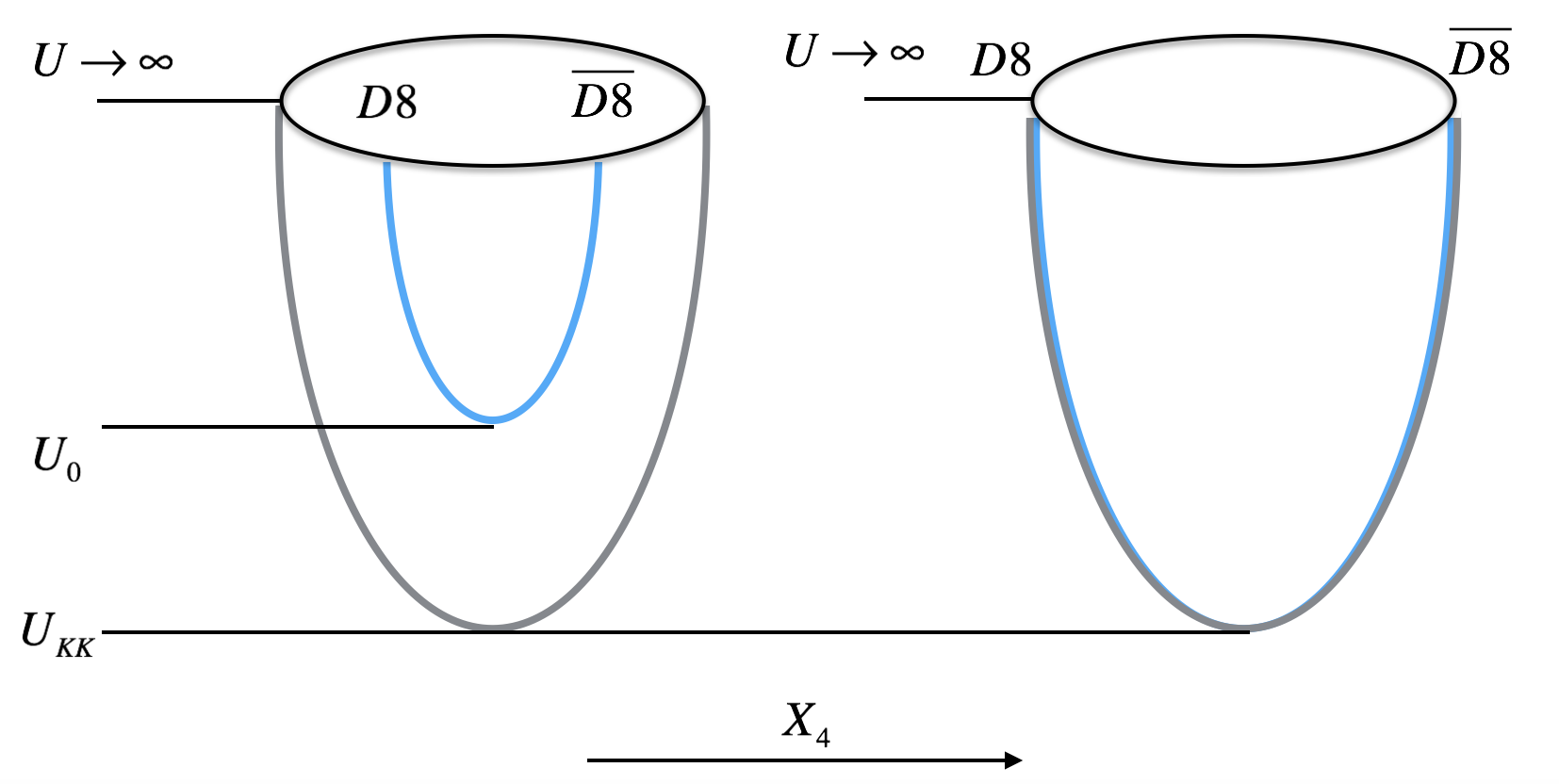
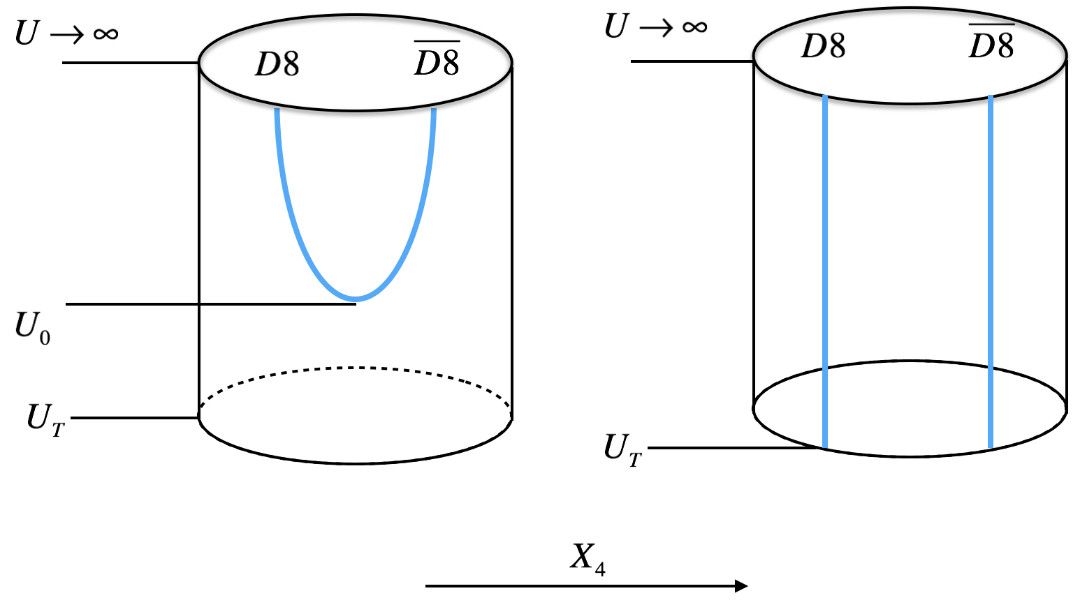
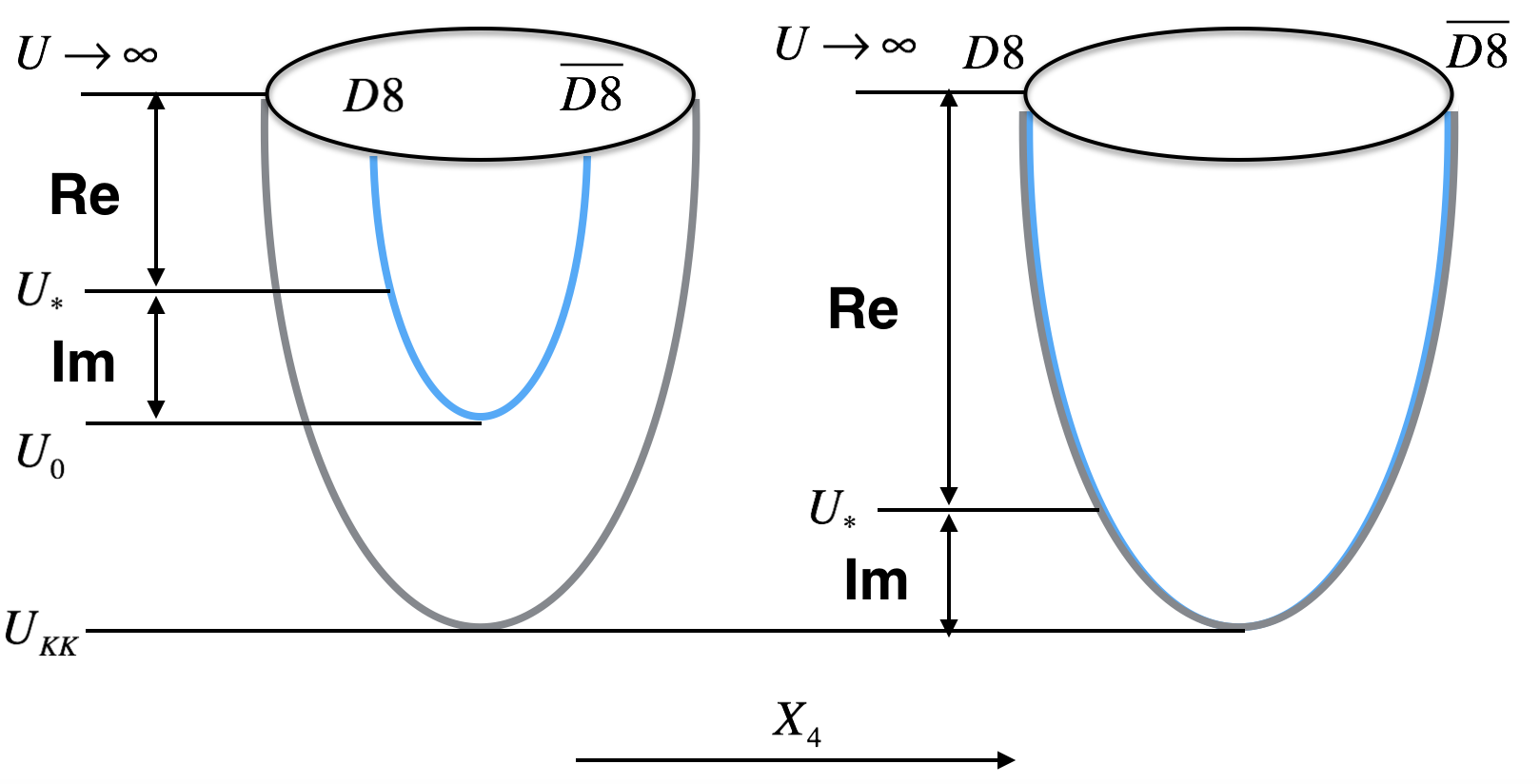
As the Witten-Sakai-Sugimoto model, the flavors could be introduced by embedding a stack of $N_{f}$ D8 and anti-D8 branes ($\mathrm{D}8/\overline{\mathrm{D}8}$-branes) as probes into the D0-D4 background (4) or (10). These $\mathrm{D}8/\overline{\mathrm{D}8}$-branes provide $U_{R}\left(N_{f}\right)\times U_{L}\left(N_{f}\right)$ symmetry as chiral symmetry holographically. It has been turned out that, in the bubble solution (4), the $\mathrm{D}8/\overline{\mathrm{D}8}$-branes are always connected which represents the chirally broken symmetry in the dual field theory. In the black brane solution (10), the configuration of $\mathrm{D}8/\overline{\mathrm{D}8}$-branes could be connected or parallel, which could be identified as the chirally broken or symmetric phase in the dual field theory respectively333The analyzing of the configuration of the $\mathrm{D}8/\overline{\mathrm{D}8}$-branes is similar as [33, 34] in the Witten-Sakai-Sugimoto model. . The various configurations of $\mathrm{D}8/\overline{\mathrm{D}8}$-branes are shown in Figure 1 and Figure 2.

Refer to caption
Figure 1: Possible configurations of $\mathrm{D}8/\overline{\mathrm{D}8}$-branes in the D0-D4 bubble background in $X_{4}-U$ plane. The $\mathrm{D}8/\overline{\mathrm{D}8}$-branes are always connected which represents the chirally broken phase in the dual field theory. The left configuration is non-antipodal while the right one is antipodal.
Refer to caption
Figure 2: Possible configurations of $\mathrm{D}8/\overline{\mathrm{D}8}$-branes in the black D0-D4 background in $X_{4}-U$ plane. In the left one, the $\mathrm{D}8/\overline{\mathrm{D}8}$-branes are connected while they are parallel in the right one, which corresponds to chirally broken and symmetric phase in the dual field theory respectively.

3 Euler-Heisenberg Lagrangian of the D0-D4/D8 brane system

In this section, we are going to derive the Euler-Heisenberg Lagrangian in bubble and black D0-D4 brane background respectively. Then we can investigate the Schwinger effect or creation of quark-antiquark.

3.1 The bubble D0-D4 geometry

In the bubble D0-D4 background, the flavored $\mathrm{D}8/\overline{\mathrm{D}8}$-branes are embedded with the following induced metric on their worldvolume,

$\displaystyle ds_{D8}^{2}$ $\displaystyle=$ $\displaystyle H_{0}^{1/2}\left(\frac{U}{R}\right)^{3/2}\eta_{\mu\nu}dX^{\text{\textmu}}dX^{\nu}+H_{0}^{1/2}\left(\frac{U}{R}\right)^{3/2}\frac{dU^{2}}{h_{c}(U)}$ (12)
$\displaystyle+$ $\displaystyle H_{0}^{1/2}\left(\frac{R}{U}\right)^{3/2}U^{2}d\Omega_{4}^{2},$

where

$\displaystyle h_{c}\left(U\right)$ $\displaystyle\equiv\left[H_{0}^{-1}f(U)\left(\frac{dX^{4}(U)}{dU}\right)^{2}+\left(\frac{R}{U}\right)^{3}\frac{1}{f(U)}\right]^{-1}.$ (13)

Notice that, for antipodal case, the D8-branes intersect $X^{4}=0$ and the anti-D8-branes put parallel at $X^{4}=\pi R_{S^{1}}$ which implies $\partial_{U}X^{4}=0$ in (13). Here, the $R_{S^{1}}$ represents the radius of $S^{1}$.

In order to evaluate the vacuum decay rate in strongly coupled gauge theory, we need to derive the Euler-Heisenberg Lagrangian and analyze its instability (i.e. find the imaginary part of the Euler-Heisenberg Lagrangian). The Euler-Heisenberg Lagrangian could be obtained from the probe brane action [13, 14, 15] since it describes the dynamics of the flavored quarks. So we shall derive the Euler-Heisenberg Lagrangian from the following probe $\mathrm{D}8/\overline{\mathrm{D}8}$-brane action with a constant electromagnetic field444The low energy effective action of a D-brane consists of two parts: Dirac-Born-Infeld (DBI) action plus Chern-Simons (CS) term. In this paper, we do not need to consider the Chern-Simons term since it has nothing to do with the electromagnetic instability.,

$$S_{D8/\overline{D8}}^{\mathrm{DBI}}=-T_{8}\int_{U_{0}}^{\infty}d^{4}XdUd\Omega_{4}e^{-\phi}\sqrt{-\det\left(P\left[g\right]_{ab}+2\pi\alpha^{\prime}F_{ab}\right)},$$ (14)

where $T_{8}$ is the D8-brane tension which is defined as $T_{8}=g_{s}^{-1}(2\pi)^{-8}l_{s}^{-9}$ and $U_{0}$ represents the connected position of the $\mathrm{D}8/\overline{\mathrm{D}8}$-branes555For the antipodal case, we need to choose $U_{0}=U_{KK}$.. For simplicity, we need to consider a single flavor $N_{f}=1$ for the presence of an external electromagnetic field. We further require the electromagnetic field is non-dynamical (i.e. constant) and their components on the $S^{4}$ are zero. Without losing generality, we could turn on the electric field on the $X^{1}$ direction only and the magnetic fields could be introduced in $X^{1},X^{2},X^{3}$ directions since the $X^{i},\ i=1,2,3$ spacial space is rotationally symmetric. Inserting constant electromagnetic field with the induced metric (12) into the DBI action (14), the effective Lagrangian is obtained as,

$$\mathcal{L}=-\frac{8\pi^{2}T_{8}}{3g_{s}}\int_{U_{0}}^{\infty}dUU^{4}H_{0}^{3/2}h_{c}^{-1/2}\sqrt{\xi_{c}},$$ (15)

where the integral of $d\Omega_{4}$ is Vol($S^{4}$)$=$ $8\pi^{2}/3$. And $\xi_{c}$ is given as,

$\displaystyle\xi_{c}=$ $\displaystyle 1-\frac{(2\pi\alpha^{\prime})^{2}R^{3}}{U^{3}H_{0}}\left[F_{01}^{2}-F_{12}^{2}-F_{23}^{2}-F_{13}^{2}+h_{c}(U)(F_{0U}^{2}-F_{1U}^{2})\right]$
$\displaystyle-\frac{(2\pi\alpha^{\prime})^{4}R^{6}}{U^{6}H_{0}^{2}}\left[F_{01}^{2}F_{23}^{2}+h_{c}(U)\left\{F_{0U}^{2}(F_{12}^{2}+F_{23}^{2}+F_{13}^{2})-F_{1U}^{2}F_{23}^{2}\right\}\right].$ (16)

Then we will derive the equations of motion from (15) respected to $A_{0}\left(U\right)$ and $A_{1}\left(U\right)$. Notice that, we could put $\partial_{i}=0,\ i=1,2,3$ since only the homogeneous phases are interesting here. In particular, we additionally require $\partial_{0}=0$ as a constraint of the static configurations, so that the equations of motion for the static (time-independent) configurations are obtained as666When both electric and magnetic fields are turned on, the Chern-Simons term in the action contributes to the equations of motion. It turns out that the equations of motion for $A_{U}$ implies the chiral anomaly. For simplicity, we can ignore this anomaly effect by interpreting our outcome as the physical values measured at $t=0$, at which $A_{U}$ vanishes as an initial condition.,

$\displaystyle\partial_{U}\left[\frac{UH_{0}^{1/2}h_{c}^{1/2}F_{0U}}{\sqrt{\xi_{c}}}\left\{1+\frac{\left(2\pi\alpha^{\prime}\right)^{2}R^{3}}{U^{3}H_{0}}\left(F_{12}^{2}+F_{13}^{2}+F_{23}^{2}\right)\right\}\right]$ $\displaystyle=0,$
$\displaystyle\partial_{U}\left[\frac{UH_{0}^{1/2}h_{c}^{1/2}F_{1U}}{\sqrt{\xi_{c}}}\left\{1+\frac{\left(2\pi\alpha^{\prime}\right)^{2}R^{3}F_{23}^{2}}{U^{3}H_{0}}\right\}\right]$ $\displaystyle=0.$ (17)

According to the equations of motion, the definition of the number density $d$ and the current $j$ reads,

$\displaystyle d=$ $\displaystyle\frac{\left(2\pi\alpha^{\prime}\right)^{2}8\pi^{2}R^{3}T_{8}}{3g_{s}}\frac{UH_{0}^{1/2}h_{c}^{1/2}F_{0U}}{\sqrt{\xi_{c}}}\left\{1+\frac{\left(2\pi\alpha^{\prime}\right)^{2}R^{3}}{U^{3}H_{0}}\left(F_{12}^{2}+F_{13}^{2}+F_{23}^{2}\right)\right\},$
$\displaystyle j=$ $\displaystyle\frac{\left(2\pi\alpha^{\prime}\right)^{2}8\pi^{2}R^{3}T_{8}}{3g_{s}}\frac{UH_{0}^{1/2}h_{c}^{1/2}F_{1U}}{\sqrt{\xi_{c}}}\left\{1+\frac{\left(2\pi\alpha^{\prime}\right)^{2}R^{3}}{U^{3}H_{0}}F_{23}^{2}\right\}.$ (18)

Substituting (15) for (18), we have

$\displaystyle\xi_{c}=$ $\displaystyle\frac{1-\frac{\left(2\pi\alpha^{\prime}\right)^{2}R^{3}}{U^{3}H_{0}}\left(F_{01}^{2}-F_{12}^{2}-F_{13}^{2}-F_{23}^{2}\right)-\frac{\left(2\pi\alpha^{\prime}\right)^{4}R^{6}}{U^{6}H_{0}^{2}}F_{01}^{2}F_{23}^{2}}{1+\frac{9g_{s}^{2}}{2^{6}\pi^{4}\left(2\pi\alpha^{\prime}\right)^{2}R^{3}T_{8}^{2}U^{5}H_{0}^{2}}\left[\frac{d^{2}}{1+\frac{\left(2\pi\alpha\prime\right)^{2}R^{3}}{U^{3}H_{0}}\left(F_{12}^{2}+F_{13}^{2}+F_{23}^{2}\right)}-\frac{j^{2}}{1+\frac{\left(2\pi\alpha^{\prime}\right)^{2}R^{3}}{U^{3}H_{0}}F_{23}^{2}}\right]}.$

Therefore the effective Lagrangian as the Euler-Heisenberg Lagrangian at zero temperature is,

$\displaystyle\mathcal{L}=-\frac{8\pi^{2}T_{8}}{3g_{s}}\int_{U_{KK}}^{\infty}dUU^{4}H_{0}^{3/2}h_{c}^{-1/2}$
$\displaystyle\times\sqrt{\frac{1-\frac{\left(2\pi\alpha^{\prime}\right)^{2}R^{3}}{U^{3}H_{0}}\left(E_{1}^{2}-\vec{B}^{2}\right)-\frac{\left(2\pi\alpha^{\prime}\right)^{4}R^{6}}{U^{6}H_{0}^{2}}E_{1}^{2}B_{1}^{2}}{1+\frac{9g_{s}^{2}}{2^{6}\pi^{4}\left(2\pi\alpha^{\prime}\right)^{2}R^{3}T_{8}^{2}U^{5}H_{0}^{2}}\left[\frac{d^{2}}{1+\frac{\left(2\pi\alpha\prime\right)^{2}R^{3}}{U^{3}H_{0}}\vec{B}^{2}}-\frac{j^{2}}{1+\frac{\left(2\pi\alpha^{\prime}\right)^{2}R^{3}}{U^{3}H_{0}}B_{1}^{2}}\right]}},$ (20)

where we have defined the constant electric and magnetic field as $F_{0i}=E_{i}$, $\epsilon_{ijk}F_{jk}=B_{i}$ and $\vec{B}^{2}=B_{1}^{2}+B_{2}^{2}+B_{3}^{2}$.

3.2 The black D0-D4 geometry

In the black D0-D4 background, there are two possible configurations for the embedded $\mathrm{D}8/\overline{\mathrm{D}8}$-branes which are connected and parallel respectively as shown in Figure 2. Generically, the induced metric on the $\mathrm{D}8/\overline{\mathrm{D}8}$-branes could be written as,

$\displaystyle ds^{2}=$ $\displaystyle\left(\frac{U}{R}\right)^{3/2}\left[-H_{0}^{-1/2}f_{T}\left(U\right)dt^{2}+H_{0}^{1/2}\delta_{ij}dX^{i}dX^{j}\right]$
$\displaystyle+\left(\frac{U}{R}\right)^{3/2}H_{0}^{1/2}\frac{dU^{2}}{h_{d}\left(U\right)}+H_{0}^{1/2}\left(\frac{R}{U}\right)^{3/2}U^{2}d\Omega_{4}^{2},$ (21)

where

$$h_{d}\left(U\right)=\left[\left(\partial_{U}X^{4}\right)^{2}+\left(\frac{R}{U}\right)^{3}\frac{1}{f_{T}\left(U\right)}\right]^{-1}.$$ (22)

For connected configuration of the $\mathrm{D}8/\overline{\mathrm{D}8}$-branes, we keep $X^{4}$ in (22) as a generic function depended on $U$, while $X^{4}$ is a constant for parallel configuration. Then similar as done in the bubble case, we could obtain the following Euler-Heisenberg Lagrangian once the induced metic (21) and the constant electromagnetic fields are adopted,

$$\mathcal{L}=-\frac{8\pi^{2}T_{8}}{3g_{s}}\int_{U_{0},\ U_{T}}^{\infty}dUU^{4}H_{0}h_{d}^{-1/2}f_{T}^{1/2}\sqrt{\xi_{d}}.$$ (23)

where

$\displaystyle\xi_{d}=$ $\displaystyle 1-\frac{(2\pi\alpha^{\prime})^{2}R^{3}}{U^{3}H_{0}f_{T}}\left[H_{0}(F_{01}^{2}+F_{0U}^{2}h_{d})-f_{T}(F_{12}^{2}+F_{13}^{2}+F_{23}^{2}+F_{1U}^{2}h_{d})\right]$
$\displaystyle-\frac{(2\pi\alpha^{\prime})^{4}R^{6}}{U^{6}H_{0}^{2}f_{T}}\left[H_{0}F_{01}^{2}F_{23}^{2}+H_{0}h_{d}F_{0U}^{2}(F_{12}^{2}+F_{13}^{2}+F_{23}^{2})-h_{d}f_{T}F_{1U}^{2}F_{23}^{2}\right].$ (24)

We have used $U_{0}$ to represent the connected position of the $\mathrm{D}8/\overline{\mathrm{D}8}$-branes. Notice that in the parallel configuration, the integral in (23) starts from $U_{T}$. Next, we could obtain the equations of motion for static (time independent) configuration which are,

$\displaystyle\partial_{U}\left[\frac{UH_{0}h_{d}^{1/2}F_{0U}}{\sqrt{f_{T}\xi_{d}}}\left\{1+\frac{\left(2\pi\alpha^{\prime}\right)^{2}R^{3}}{U^{3}H_{0}}\left(F_{12}^{2}+F_{13}^{2}+F_{23}^{2}\right)\right\}\right]$ $\displaystyle=0,$
$\displaystyle\partial_{U}\left[\frac{Uh_{d}^{1/2}f_{T}^{1/2}F_{1U}}{\sqrt{\xi_{d}}}\left(1+\frac{\left(2\pi\alpha^{\prime}\right)^{2}R^{3}}{U^{3}H_{0}}F_{23}^{2}\right)\right]$ $\displaystyle=0.$ (25)

So we have the charge density $d$ and current $j$ defined as,

$\displaystyle d$ $\displaystyle=\frac{\left(2\pi\alpha^{\prime}\right)^{2}8\pi^{2}R^{3}T_{8}}{3g_{s}}\frac{UH_{0}h_{d}^{1/2}F_{0U}}{\sqrt{f_{T}\xi_{d}}}$
$\displaystyle\left\{1+\frac{\left(2\pi\alpha^{\prime}\right)^{2}R^{3}}{U^{3}H_{0}}\left(F_{12}^{2}+F_{13}^{2}+F_{23}^{2}\right)\right\},$
$\displaystyle j$ $\displaystyle=\frac{\left(2\pi\alpha^{\prime}\right)^{2}8\pi^{2}R^{3}T_{8}}{3g_{s}}\frac{Uh_{d}^{1/2}f_{T}^{1/2}F_{1U}}{\sqrt{\xi_{d}}}\left[1+\frac{\left(2\pi\alpha^{\prime}\right)^{2}R^{3}}{U^{3}H_{0}}F_{23}^{2}\right].$ (26)

Therefore the on shell effective Lagrangian (23) contains the following form,

$$\xi_{d}=\frac{1-\frac{\left(2\pi\alpha^{\prime}\right)^{2}R^{3}}{U^{3}H_{0}f_{T}}\left[H_{0}F_{01}^{2}-f_{T}\left(F_{12}^{2}+F_{13}^{2}+F_{23}^{2}\right)\right]-\frac{\left(2\pi\alpha^{\prime}\right)^{4}R^{6}}{U^{6}H_{0}f_{T}}F_{01}^{2}F_{23}^{2}}{1+\frac{3^{2}g_{s}^{2}}{2^{6}\pi^{4}\left(2\pi\alpha^{\prime}\right)^{2}R^{3}T_{8}^{2}U^{5}H_{0}^{2}f_{T}}\left[\frac{d^{2}f_{T}}{1+\frac{\left(2\pi\alpha^{\prime}\right)^{2}R^{3}}{U^{3}H_{0}}\left(F_{12}^{2}+F_{13}^{2}+F_{23}^{2}\right)}-\frac{j^{2}H_{0}}{1+\frac{\left(2\pi\alpha^{\prime}\right)^{2}R^{3}}{U^{3}H_{0}}F_{23}^{2}}\right]}.$$ (27)

Accordingly, the Euler-Heisenberg Lagrangian at finite temperature is,

$\displaystyle\mathcal{L}=-\frac{8\pi^{2}T_{8}}{3g_{s}}\int_{U_{0},\ U_{T}}^{\infty}dUU^{4}H_{0}h_{d}^{-1/2}f_{T}^{1/2}$
$\displaystyle\times\sqrt{\frac{1-\frac{\left(2\pi\alpha^{\prime}\right)^{2}R^{3}}{U^{3}H_{0}f_{T}}\left[H_{0}E_{1}^{2}-f_{T}\vec{B}^{2}\right]-\frac{\left(2\pi\alpha^{\prime}\right)^{4}R^{6}}{U^{6}H_{0}f_{T}}E_{1}^{2}B_{1}^{2}}{1+\frac{3^{2}g_{s}^{2}}{2^{6}\pi^{4}\left(2\pi\alpha^{\prime}\right)^{2}R^{3}T_{8}^{2}U^{5}H_{0}^{2}f_{T}}\left[\frac{d^{2}f_{T}}{1+\frac{\left(2\pi\alpha^{\prime}\right)^{2}R^{3}}{U^{3}H_{0}}\vec{B}^{2}}-\frac{j^{2}H_{0}}{1+\frac{\left(2\pi\alpha^{\prime}\right)^{2}R^{3}}{U^{3}H_{0}}B_{1}^{2}}\right]}},$ (28)

where the definitions of $E_{i}$ and $B_{i}$ are as same as in the bubble case.

4 Holographic pair creation of quark-antiquark

In the previous sections, we have obtained the effective Euler-Heisenberg Lagrangian both in the bubble and black D0-D4 brane geometry. In this section, let us compute the imaginary part of the action in order to evaluate the pair creation of quark-antiquark holographically at zero or finite temperature. For simplicity, we will be interested in looking at the instability of the vacuum as [13, 14, 15].

4.1 Imaginary part of the effective action at zero temperature

Since the bubble D0-D4 geometry holographically corresponds to the confinement phase of the dual field theory at zero temperature, let us evaluate the imaginary part of the action (20) from the bubble D0-D4 geometry first. For the vacuum case, by setting $d=j=0$, the Lagrangian (20) takes the following form,

$$\mathcal{L}=-\frac{8\pi^{2}T_{8}}{3g_{s}}\int_{U_{0},\ U_{KK}}^{\infty}dUU^{4}H_{0}^{3/2}h_{c}^{-1/2}\sqrt{1-\frac{\left(2\pi\alpha^{\prime}\right)^{2}R^{3}}{U^{3}H_{0}}\left(E_{1}^{2}-\vec{B}^{2}\right)-\frac{\left(2\pi\alpha^{\prime}\right)^{4}R^{6}}{U^{6}H_{0}^{2}}E_{1}^{2}B_{1}^{2}}.$$ (29)

The critical position for $U=U_{*}$ , where the imaginary part of the Lagrangian (29) appears, obviously satisfies the equation,

$$\frac{\left(2\pi\alpha^{\prime}\right)^{4}R^{6}}{U_{*}^{6}H_{0}\left(U_{*}\right)^{2}}E_{1}^{2}B_{1}^{2}+\frac{\left(2\pi\alpha^{\prime}\right)^{2}R^{3}}{U_{*}^{3}H_{0}\left(U_{*}\right)}\left(E_{1}^{2}-\vec{B}^{2}\right)-1=0.$$ (30)

After solving (30) we therefore obtain,

$$U_{*}=\left\{\frac{\left(2\pi\alpha^{\prime}\right)^{2}R^{3}}{2}\left[E_{1}^{2}-\vec{B}^{2}+\sqrt{\left(\vec{B}^{2}-E_{1}^{2}\right)^{2}+4B_{1}^{2}E_{1}^{2}}\right]-U_{Q_{0}}^{3}\right\}^{1/3}.$$ (31)

So it is clear that in the region of $U$ : $U_{0}\leq U\leq U_{*}$ , the Lagrangian is imaginary as shown in Figure 3.

Refer to caption
Figure 3: The region of the integral in the imaginary Lagrangian of the $\mathrm{D}8/\overline{\mathrm{D}8}$-branes in the bubble D0-D4 background. Left: In the non-antipodal case, the integral in the imaginary Lagrangian starts from $U_{0}$ to $U_{*}$. Right: In the antipodal case the integral in the imaginary Lagrangian starts from $U_{KK}$ to $U_{*}$.

Since the creation rate of the quark-antiquark is proportional to the imaginary part of the Lagrangian (29), next we are going to examine whether or not the imaginary part diverges. By the neighborhood of $U_{0}$, we assume $U_{*}=U_{0}+\varepsilon$ where $\varepsilon\ll U_{0}$ as [13]. Then the imaginary part of (29) can be rewritten in terms of the expansion near $U_{0}$ as,

$\displaystyle\mathrm{Im}\mathcal{L}=$ $\displaystyle-\frac{8\pi^{2}T_{8}}{3g_{s}}\int_{U_{0},U_{KK}}^{U_{*}}dUU^{4}H_{0}^{3/2}h_{c}^{-1/2}\sqrt{\frac{\left(2\pi\alpha^{\prime}\right)^{4}R^{6}}{U^{6}H_{0}^{2}}E_{1}^{2}B_{1}^{2}+\frac{\left(2\pi\alpha^{\prime}\right)^{2}R^{3}}{U^{3}H_{0}}\left(E_{1}^{2}-\vec{B}^{2}\right)-1}$
$\displaystyle\simeq$ $\displaystyle-\frac{8\pi^{2}T_{8}}{3g_{s}}\mathcal{F}\left(U_{0}\right)\underset{U_{*}\rightarrow U_{0}}{\lim}\left[\left(U_{*}-U_{0}\right)\times h_{c}^{-1/2}\left(U_{0}\right)\right]$
$\displaystyle\simeq$ $\displaystyle-\frac{8\pi^{2}T_{8}}{3g_{s}}\mathcal{F}\left(U_{0}\right)\left[H_{0}^{-1}\left(U_{0}\right)f(U_{0})\left[X^{4}\left(U_{0}+\varepsilon\right)-X^{4}\left(U_{0}\right)\right]^{2}+\frac{R^{3}\varepsilon^{2}}{\left(U_{0}+\varepsilon\right)^{3}-U_{KK}^{3}}\right]^{1/2},$ (32)

where $\mathcal{F}\left(U\right)$ is defined as,

$$\mathcal{F}(U)=U^{4}H_{0}^{3/2}\sqrt{\frac{(2\pi\alpha^{\prime})^{4}R^{6}}{U^{6}H_{0}^{2}}E_{1}^{2}B_{1}^{2}+\frac{(2\pi\alpha^{\prime})^{2}R^{3}}{U^{3}H_{0}}(E_{1}^{2}-\vec{B}^{2})-1}.$$ (33)

Consequently (32) is finite for the non-antipodal case (i.e. $U_{0}>U_{KK}$). Moreover, in the antipodal case, we must require $U_{0}=U_{KK}$. So $X^{4}\left(U_{0}+\varepsilon\right)-X^{4}\left(U_{0}\right)$ vanishes since $X^{4}$ is a constant. Thus (32) could be simplified as,

$\displaystyle\mathrm{Im}\mathcal{L}\simeq$ $\displaystyle\frac{8\pi^{2}T_{8}R^{3/2}}{3g_{s}}\mathcal{F}\left(U_{KK}\right)\frac{\varepsilon}{\sqrt{\left(U_{KK}+\varepsilon\right)^{3}-U_{KK}^{3}}}$
$\displaystyle\simeq$ $\displaystyle\frac{8\pi^{2}T_{8}R^{3/2}}{3g_{s}U_{KK}}\mathcal{F}\left(U_{KK}\right)\left[\sqrt{\frac{\varepsilon}{3}}+\mathcal{O}\left(\varepsilon^{3/2}\right)\right]=\mathrm{finite}.$ (34)

So (32) shows a finite value for the creation rate of quark-antiquark in our D0-D4/D8 system which is due to the confining scale $U_{KK}$. If setting $U_{Q_{0}}=0$ (i.e. no smeared D0-branes or vanished $\theta$ angle), our result returns to the approximated approach in the Witten-Sakai-Sugimoto model as [13]. Accordingly, it is natural to treat (32) as a holographically generic form of the creation rate of quark-antiquark which is dependent on the topological charge from the QCD vacuum.

Since the creation of the quark antiquark breaks the vacuum, we need to evaluate the critical electric field. By the condition that the Lagrangian (32) begins to be imaginary, the critical electric field could be derived by solving,

$$U_{0}=U_{*}=\left\{\frac{\left(2\pi\alpha^{\prime}\right)^{2}R^{3}}{2}\left[E_{1}^{2}-\vec{B}^{2}+\sqrt{\left(\vec{B}^{2}-E_{1}^{2}\right)^{2}+4B_{1}^{2}E_{1}^{2}}\right]-U_{Q_{0}}^{3}\right\}^{1/3}.$$ (35)

Thus the critical electric field is,

$$E_{cr}=\left[\frac{U_{0}^{3}+U_{Q_{0}}^{3}}{\left(2\pi\alpha^{\prime}\right)^{2}R^{3}}\frac{\left\{\frac{U_{0}^{3}+U_{Q_{0}}^{3}}{\left(2\pi\alpha^{\prime}\right)^{2}R^{3}}+\vec{B}^{2}\right\}}{\left\{\frac{U_{0}^{3}+U_{Q_{0}}^{3}}{\left(2\pi\alpha^{\prime}\right)^{2}R^{3}}+B_{1}^{2}\right\}}\right]^{1/2}.$$ (36)

We find the critical electric field does not depend on $B_{1}$ if setting $B_{2},B_{3}=0$. Besides, if we look at the antipodal case which means $U_{0}=U_{KK}$, and substitute (36) for (9), then the critical electric field could be obtained as,

$$E_{cr}=\frac{2}{27\pi}\lambda M_{KK}^{2}\left(1+\zeta\right)^{2}\left[\frac{\frac{4}{3^{6}\pi^{2}}\lambda^{2}M_{KK}^{4}\left(1+\zeta\right)^{4}+\vec{B}^{2}}{\frac{4}{3^{6}\pi^{2}}\lambda^{2}M_{KK}^{4}\left(1+\zeta\right)^{4}+B_{1}^{2}}\right]^{1/2}.$$ (37)

where $\zeta$ is defined as $\zeta=U_{Q_{0}}^{3}/U_{KK}^{3}$. Since $\zeta$ is related to the D0-brane density, (37) shows the dependence on the $\theta$ angle from the QCD vacuum. And it coincides with the generic formula in [13] if setting $\zeta=0$. Notice that if $B_{2}=B_{3}=0$, the critical electric field is $E_{cr}=\frac{2}{27\pi}\lambda M_{KK}^{2}\left(1+\zeta\right)^{2}$ which increases by the appearance of the $\theta$ angle (i.e. D0 charge).

In order to evaluate the imaginary part of the Lagrangian (29) numerically, let us derive the expression of (29) by using the following dimensionless variables. Introducing the dimensionless variables as,

$$U=\frac{U_{KK}}{yH_{KK}H_{0}^{1/3}}=\frac{\left(U_{KK}^{3}-H_{KK}^{3}U_{Q_{0}}^{3}y^{3}\right)^{1/3}}{yH_{KK}},$$ (38)

and substituting (29) for (9) and (38), we obtain,

$\displaystyle\mathrm{Im}\mathcal{L}=$ $\displaystyle\frac{M_{KK}^{4}\lambda^{3}N_{c}}{2\cdot 3^{8}\pi^{5}}\int_{y_{*}}^{y_{0},y_{kk}}dy\left\{1+y\left[1-y^{3}\zeta\left(1+\zeta\right)^{3}\right]^{4/3}\left[1-y^{3}\left(1+\zeta\right)^{4}\right]^{2}x_{4}^{\prime 2}\right\}^{1/2}$
$\displaystyle\times y^{-9/2}\left[1-y^{3}\zeta\left(1+\zeta\right)^{3}\right]^{-5/6}\left[1-y^{3}\left(1+\zeta\right)^{4}\right]^{-1/2}\sqrt{y^{6}\boldsymbol{\mathrm{E}}_{1}^{2}\boldsymbol{\mathrm{B}}_{1}^{2}+y^{3}\left(\boldsymbol{\mathrm{E}}_{1}^{2}-\vec{\boldsymbol{\mathrm{B}}}^{2}\right)-1},$ (39)

where

$$y_{kk}=\left(1+\zeta\right)^{-4/3},y_{*}=\frac{U_{KK}}{\left(1+\zeta\right)\left(U_{*}^{3}+U_{Q_{0}}^{3}\right)^{1/3}},\ \ X_{4}=\frac{3x_{4}}{2M_{KK}},\boldsymbol{\mathrm{E}}_{i}=\frac{3^{3}\pi}{2\lambda M_{KK}^{2}}E_{i},\ \boldsymbol{\mathrm{B}}_{i}=\frac{3^{3}\pi}{2\lambda M_{KK}^{2}}B_{i}.$$

Notice that we need to obtain the exact formula for $x_{4}$ in (39) by solving its equation of motion before the numerical calculations, however, which would become very challenging. So in this paper, we will not attempt to evaluate (39) with the exact solution for $x_{4}$. Instead, as a typical exploration, we evaluate the imaginary part (29) in the antipodal case for simplicity777In some limit, the contribution from $x_{4}^{\prime}$ to the effective Lagrangian is not important. For example, if $\varepsilon\rightarrow 0$ in (32), we obtain $X^{4}\left(U_{0}+\varepsilon\right)\simeq X^{4}\left(U_{0}\right)$. Therefore in this limit, $x_{4}^{\prime}$ does not contribute to the effective Lagrangian (32).. Moreover, we interestingly find that (39) may show an additionally possible instability because the second line of (39) could also be imaginary and it does not depend on the electromagnetic field. Since the bubble D0-D4/D8 system corresponds to a confining Yang-Mills theory with a topological Chern-Simons term, so the instability produced by $\theta$ angle (i.e. D0 charge) could be holographically interpreted as the transition between the different $\theta$ vacuum states, which has been very well-known in QCD. However in order to investigate the electromagnetic instability, we need to remove the $\theta$-instability from the vacuum. Hence we expand (39) by $\zeta$ since $\theta$ angle in QCD is very small. Therefore in the antipodal case (i.e. $x_{4}^{\prime}=0$) with small $\zeta$ expansion, we obtain the following formula for the imaginary Lagrangian,

$\displaystyle\mathrm{Im}\mathcal{L}\simeq$ $\displaystyle\frac{M_{KK}^{4}\lambda^{3}N_{c}}{2\cdot 3^{8}\pi^{5}}\int_{y_{*}}^{y_{kk}}dy\sqrt{y^{6}\boldsymbol{\mathrm{E}}_{1}^{2}\boldsymbol{\mathrm{B}}_{1}^{2}+y^{3}\left(\boldsymbol{\mathrm{E}}_{1}^{2}-\vec{\boldsymbol{\mathrm{B}}}^{2}\right)-1}$
$\displaystyle\times y^{-9/2}\left[\frac{1}{\sqrt{1-y^{3}}}-\frac{y^{3}\left(5y^{3}-17\right)}{6\left(1-y^{3}\right)^{3/2}}\zeta\right].$ (40)

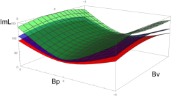
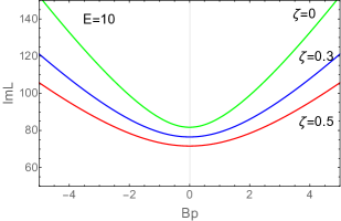
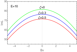
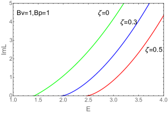
The (40) could be numerically evaluated and the result is shown in Figure 4. We plot the $\mathrm{Im}L$ as a function of $\zeta$, the dimensionless magnetic field $B_{\mathrm{P}}$ and $B_{\mathrm{V}}$ which is parallel and perpendicular to the (dimensionless) electric field $\boldsymbol{\mathrm{E}}$. In Figure 4, we use different colors, as red, blue and green, to distinguish the dependence on $\zeta$ ($\theta$ angle) with $\zeta=0.5,\ 0.3,\ 0$ respectively. It shows if the magnetic field and the electric field are parallel, the imaginary part of the Lagrangian increases as the magnetic field increases. And on the other hand, if the magnetic field and the electric field is perpendicular to each other, the imaginary part of the Lagrangian decreases when the magnetic field increases. The relation between $\mathrm{Im}L$ and parallel/perpendicular magnetic field with different $\zeta$ is shown in Figure 5.

Refer to caption
Figure 4: The imaginary part of the effective Lagrangian with a fixed $E$ as a function of $\zeta$, the magnetic field $B_{\mathrm{P}}$ and $B_{\mathrm{V}}$ which is parallel and perpendicular to the electric field $E$. In this figure, we look at $\boldsymbol{\mathrm{E}}_{1}=\mathrm{E}=10$ with $\zeta=0.5,\ 0.3,\ 0$ represented by red, blue and green respectively. It shows the dependence on $\zeta$ ($\theta$ angle) and the imaginary part of the Lagrangian decreases if $\zeta$ increases.
Refer to caption
Refer to caption
Figure 5: Relation between $\mathrm{Im}L$ and $B_{\mathrm{V}},\ B_{\mathrm{P}}$ with different $\zeta$. If $\zeta$ increases, $\mathrm{Im}L$ decreases. Left: The magnetic field is parallel to the electric field and $\mathrm{Im}L$ increases as the magnetic field increases. Right: The magnetic field is perpendicular to the electric field and $\mathrm{Im}L$ decreases as the magnetic field increases.

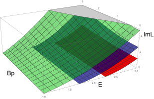
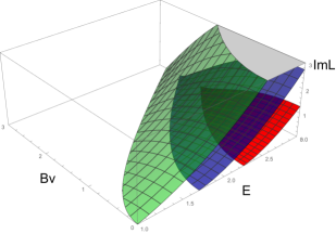
We furthermore look at the dependence on $E$ with various $\zeta$ in the case of a parallel/perpendicular magnetic field respectively. The numerical evaluation is summarized in Figure 6. Accordingly, we could conclude that, in the bubble D0-D4 system, the electromagnetic instability is suppressed by the appearance of D0 charge ($\theta$ angle in QCD), however with a fixed $\zeta$, its behavior depends on the direction of the magnetic field relative to the electric field. Finally, we also plot the relation between the electric field with an arbitrary magnetic field to confirm our conclusion which is shown in Figure 7.

Refer to caption
Refer to caption
Figure 6: In this figure, red blue and green represent $\zeta=0.5,\ 0.3,\ 0$ respectively as before. Left: The magnetic field is parallel to the electric field. Right: The magnetic field is perpendicular to the electric field.
Refer to caption
Figure 7: The relation between $\mathrm{Im}L$ with an arbitrary magnetic field and various $\zeta$.

4.2 Imaginary part of the action at finite temperature

In the previous section, we have obtained the effective action from the black D0-D4 background i.e. at finite temperature. Since we are most interested in the vacuum instability, it would be suitable to set the charge density and current vanished in the Lagrangian (28) i.e. $d=j=0$ . Then we obtain the simplified Lagrangian from (28) which is,

$\displaystyle\mathcal{L}=$ $\displaystyle-\frac{8\pi^{2}T_{8}}{3g_{s}}\int_{U_{0},U_{T}}^{\infty}dUU^{4}H_{0}h_{d}^{-1/2}f_{T}^{1/2}$
$\displaystyle\times\sqrt{1-\frac{\left(2\pi\alpha^{\prime}\right)^{2}R^{3}}{U^{3}H_{0}f_{T}}\left[H_{0}E_{1}^{2}-f_{T}\vec{B}^{2}\right]-\frac{\left(2\pi\alpha^{\prime}\right)^{4}R^{6}}{U^{6}H_{0}f_{T}}E_{1}^{2}B_{1}^{2}}.$ (41)

We can evaluate the imaginary part of the Lagrangian to derive the rate of the quark antiquark creation in the vacuum by (41).

To begin with, let us consider the case of zero-temperature limit, i.e. $U_{T}\rightarrow 0$, so that the function $f_{T}\left(U\right)$ approaches unity. The third term in the square root of the Lagrangian (41) must be dominated because the integral in (41) should be totally imaginary. Thus the $U$-integral is finite. Accordingly, in the presence of the electromagnetic field, the vacuum decay rate is finite at strong coupling in the zero temperature limit in our D0-D4/D8 system or the Witten-Sakai-Sugimoto model. Then let us compute it in details. Introducing the dimensionless variables as,

$$y=\frac{U_{T}}{UH_{T}H_{0}^{1/3}},\ \zeta_{T}=\frac{U_{Q_{0}}^{3}}{U_{T}^{3}},\ \chi=\frac{U_{T}^{3}}{\left(2\pi\alpha^{\prime}\right)^{2}R^{3}},\ x_{4}=\frac{3}{2}\frac{3U_{T}^{1/2}}{2R^{3/2}}H_{T}^{-1/2}X^{4},$$ (42)

we have,

$\displaystyle\mathcal{L}=$ $\displaystyle-\frac{2^{3}\pi^{2}\left(2\pi\alpha^{\prime}\right)^{7/3}R^{5}T_{8}}{3g_{s}}\chi^{7/6}\left(1+\zeta_{T}\right)^{-1/2}\int_{y_{T},y_{0}}^{0}dyy^{-9/2}\left[1-y^{3}\zeta_{T}\left(1+\zeta_{T}\right)^{3}\right]^{-5/6}$
$\displaystyle\times\left\{y\left[1-y^{3}\left(1+\zeta_{T}\right)^{4}\right]\left[1-y^{3}\zeta_{T}\left(1+\zeta_{T}\right)^{3}\right]^{4/3}x_{4}^{\prime 2}+1\right\}^{1/2}$
$\displaystyle\times\sqrt{\left(1+\zeta_{T}\right)^{-6}-\frac{y^{3}}{\chi}\left\{E_{1}^{2}\left[1-y^{3}\left(1+\zeta_{T}\right)^{4}\right]^{-1}-\vec{B}^{2}\right\}\left(1+\zeta_{T}\right)^{-3}-\frac{y^{6}}{\chi^{2}}E_{1}^{2}B_{1}^{2}\left[1-y^{3}\left(1+\zeta_{T}\right)^{4}\right]^{-1}},$ (43)

where $y_{T}=\left(1+\zeta_{T}\right)^{-4/3}$ and $H_{T}\equiv H_{0}\left(U_{T}\right)$. Further rescale $Y=\chi^{-1/3}y$, it yields,

$\displaystyle\mathrm{Im}\mathcal{L}=$ $\displaystyle-\frac{2^{3}\pi^{2}\left(2\pi\alpha^{\prime}\right)^{7/3}R^{5}T_{8}}{3g_{s}}\left(1+\zeta_{T}\right)^{-7/2}\int_{\chi^{-1/3}\left(1+\zeta_{T}\right)^{-4/3}}^{Y_{*}}dYY^{-9/2}\bigg{\{}\left[B_{1}^{2}E_{1}^{2}\left(1+\zeta_{T}\right)^{6}+\vec{B}^{2}\left(1+\zeta_{T}\right)^{7}\chi\right]Y^{6}$
$\displaystyle+\left[\left(1+4\zeta_{T}+6\zeta_{T}^{2}+4\zeta_{T}^{3}+\zeta_{T}^{4}\right)\chi+\left(E_{1}^{2}-\vec{B}^{2}\right)\left(1+\zeta_{T}\right)^{3}\right]Y^{3}-1\bigg{\}}^{1/2}$
$\displaystyle\times\bigg{\{}1+\chi^{1/3}Y\left[1-Y^{3}\zeta_{T}\left(1+\zeta_{T}\right)^{3}\chi\right]^{4/3}\left[1-Y^{3}\left(1+\zeta_{T}\right)^{4}\chi\right]x_{4}^{\prime 2}\bigg{\}}^{1/2}\left[1-Y^{3}\zeta_{T}\left(1+\zeta_{T}\right)^{3}\chi\right]^{-5/6}$
$\displaystyle\times\left[1-Y^{3}\left(1+\zeta_{T}\right)^{4}\chi\right]^{-1/2}.$ (44)

Since there are two possible configurations for $\mathrm{D}8/\overline{\mathrm{D}8}$-branes in the black brane background as shown in Figure 2, let us consider the parallel $\mathrm{D}8/\overline{\mathrm{D}8}$-branes first, i.e. $x_{4}^{\prime}=0$. In the small temperature limit $\chi\rightarrow 0$, the third term in the square root of the Lagrangian (41) become dominated, so that we have the following behavior from (44),

$\displaystyle\mathrm{Im}\mathcal{L}\simeq$ $\displaystyle-\frac{2^{3}\pi^{2}\left(2\pi\alpha^{\prime}\right)^{7/3}R^{5}T_{8}}{3g_{s}}\vec{E}\cdot\vec{B}\left(1+\zeta_{T}\right)^{-1/2}\int_{\chi^{-1/3}\left(1+\zeta_{T}\right)^{-4/3}}^{Y_{*}}dYY^{-3/2}$
$\displaystyle\times\left[1-Y^{3}\zeta_{T}\left(1+\zeta_{T}\right)^{3}\chi\right]^{-5/6}\left[1-Y^{3}\zeta_{T}\left(1+\zeta_{T}\right)^{4}\chi\right]^{-1/2}$
$\displaystyle\simeq$ $\displaystyle\frac{2^{4}\pi^{2}\left(2\pi\alpha^{\prime}\right)^{7/3}R^{5}T_{8}}{3g_{s}\sqrt{1+\zeta_{T}}}\vec{B}\cdot\vec{E}Y_{*}^{-1/2}+\mathcal{O}\left(\chi^{1/6}\right)=\mathrm{finite}.$ (45)

where $Y_{*}$ satisfies the following equation in the small $\chi$ limit,

$$1-\left(E_{1}^{2}-\vec{B}^{2}\right)Y_{*}^{3}-\left(B_{1}E_{1}\right)^{2}Y_{*}^{6}=0,$$ (46)

so that if the magnetic field is parallel to the electric field, we have $Y_{*}=E_{1}^{-2/3}$. According to (45), the creation rate decreases when $\zeta_{T}$ increases. It coincides with our result in bubble case. Moreover, the generic solution of (46) can be found as,

$$Y_{*}=\left[\frac{\vec{E}^{2}-\vec{B}^{2}+\sqrt{\left(\vec{E}^{2}-\vec{B}^{2}\right)^{2}+4\left(\vec{E}\cdot\vec{B}\right)^{2}}}{2}\right]^{-1/3}.$$ (47)
Refer to caption
Figure 8: The region of the integral in the imaginary Lagrangian of the D8/D8-branes in the black D0-D4 background. Left: The configuration of D8/D8-branes is “U” shape, thus the integral in the imaginary Lagrangian starts from $U_{0}$ to $U_{\ast}$. Right: The configuration of D8/D8-branes is parallel and the integral in the imaginary Lagrangian starts from $U_{T}$ to $U_{\ast}$.

On the other hand, for the connected configuration of $\mathrm{D}8/\overline{\mathrm{D}8}$-branes, taking the zero temperature limit $U_{T}\rightarrow 0$, we have,

$$y_{0}=\frac{U_{T}}{U_{0}H_{T}H_{0}^{1/3}\left(U_{0}\right)}\rightarrow 0.$$ (48)

Thus the imaginary part of the Lagrangian contains the integral starting from $Y_{0}$ to $Y_{*}$ (i.e. $U_{0}$ to $U_{*}$) with $Y_{0}\rightarrow Y_{*}$. As the previous section, we can expand $Y$ (or $y$) in the neighborhood $Y_{*}\simeq Y_{0}+\varepsilon$ where $\varepsilon\ll Y_{0}$. Since in the connected configuration of the $\mathrm{D}8/\overline{\mathrm{D}8}$-branes, $x_{4}$ is a function of $y$, we obtain the following behavior of the imaginary Lagrangian in the small temperature limit $\chi\rightarrow 0$,

$\displaystyle\mathrm{Im}\mathcal{L}\simeq$ $\displaystyle-\frac{2^{3}\pi^{2}\left(2\pi\alpha^{\prime}\right)^{7/3}R^{5}T_{8}}{3g_{s}}\vec{E}\cdot\vec{B}\left(1+\zeta_{T}\right)^{-1/2}\mathcal{G}\left(Y_{0}\right)$
$\displaystyle\times\bigg{\{}1+\chi^{1/3}Y_{0}\left[1-Y_{0}^{3}\zeta_{T}\left(1+\zeta_{T}\right)^{3}\chi\right]^{4/3}\left[1-Y_{0}^{3}\left(1+\zeta_{T}\right)^{4}\chi\right]x_{4}^{\prime 2}\left(Y_{0}\right)\bigg{\}}^{1/2}\varepsilon$
$\displaystyle=$ $\displaystyle-\frac{2^{3}\pi^{2}\left(2\pi\alpha^{\prime}\right)^{7/3}R^{5}T_{8}}{3g_{s}}\vec{E}\cdot\vec{B}\left(1+\zeta_{T}\right)^{-1/2}\mathcal{G}\left(Y_{0}\right)$
$\displaystyle\times\bigg{\{}\varepsilon^{2}+\chi^{1/3}Y_{0}\left[1-Y_{0}^{3}\zeta_{T}\left(1+\zeta_{T}\right)^{3}\chi\right]^{4/3}\left[1-Y_{0}^{3}\left(1+\zeta_{T}\right)^{4}\chi\right]\left[x_{4}\left(Y_{0}+\varepsilon\right)-x_{4}\left(Y_{0}\right)\right]^{2}\bigg{\}}^{1/2}=\mathrm{finite},$ (49)

where

$\displaystyle\mathcal{G}\left(Y\right)=$ $\displaystyle Y^{-3/2}\left[1-Y^{3}\zeta_{T}\left(1+\zeta_{T}\right)^{3}\chi\right]^{-5/6}$
$\displaystyle\left[1-Y^{3}\zeta_{T}\left(1+\zeta_{T}\right)^{4}\chi\right]^{-1/2}.$ (50)

Therefore according to the evaluation, the imaginary part of the effective Lagrangian is always finite at zero temperature limit. We have also confirmed our conclusion numerically with arbitrary temperature. It would be very interesting to compare our calculations in this section with the D3/D7 approach in [14, 15]. The creation of quark-antiquark is proportional to $\log\frac{1}{T}$ in [14, 15] which diverges at zero temperature limit, while it is always finite in our D0-D4/D8 system or the original Witten-Sakai-Sugimoto model. However, this result is not surprised because there is a confining scale in the compactified D4-brane (with or without smeared D0-branes) system as (7) or (8), and on the other hand the bubble configuration would be thermodynamically dominated at low temperature while the black brane configuration arises at high temperature [31, 33, 34, 35]. Consequently our calculation in the black D0-D4 configuration (high temperature) consistently coincides with the case in bubble D0-D4 (low temperature) at zero temperature limit, which means the creation rate should be definitely finite. Besides, as the situation of bubble D0-D4 system, we also find an additionally possible instability based on our calculations in (43) since the first line in (43) may also be imaginary. So it is the instability from the vacuum without the electromagnetic field as discussed in the bubble case.

5 Summary and discussion

In this paper, we have studied the electromagnetic instability by deriving the effective Euler-Heisenberg Lagrangian for the flavored quarks in the Witten-Sakai-Sugimoto model with the D0-D4 background. Since the dynamics of the flavored quarks is described by the DBI action of the probe $\mathrm{D8/\overline{D8}}$-branes, we identify its DBI action with the constant electromagnetic fields as the effective Euler-Heisenberg action. Then we explore the electromagnetic instability and evaluated the pair creation rate of quark-antiquark in the Schwinger effect. With the D0-D4/D8 model in string theory, our investigation contains the influence of the D0-brane density which could be interpreted as the $\theta$ angle or chiral potential in QCD. In the bubble configuration, since the D4-branes with smeared D0-branes are wrapped on a cycle, it introduces a confining scale into this system. Therefore, we obtain a very different result from $\mathcal{N}=2$ supersymmetric QCD in the approach of D3/D7 [14, 15].

In order to investigate the electromagnetic instability, we assume the electromagnetic field is sufficient strong, then we find the $\theta$-dependent creation rate of flavored quark-antiquark obtained in the bubble D0-D4 background exactly coincides with [13] if setting $\theta$ angle or $\zeta=0$ (i.e. no D0-branes). Our numerical calculation also shows the creation rate decreases when $\theta$ angle or $\zeta$ increases and its behavior depends on the direction of the magnetic field relative to the electric field. To understand this, let us combine our results with [25, 27, 28, 29]. Since the critical electric field evaluated in (37) is in quantitative agreement with the mass spectrum in [25, 27, 28, 29] which describes the possible metastable states in the heavy-ion collision, our results imply that in the heavy-ion collision the metastable state could be created in the Schwinger effect then it soon decays to the true vacuum as discussed in [41, 42]. And because of the condensate of gluon, these metastable states become heavier, so the critical electric field increases while its associated decay rate decreases in the present of D0-branes i.e. $\theta$ angle.

Moreover, the creation rate in the black D0-D4 background has also been computed which remains to be finite while it is oppose to the D3/D7 approach [14, 15]. Nevertheless, our result would be significant. Since the Hawking-Page transition in the WSS model is usually interpreted as confined/deconfined phase transition in QCD [31, 35], it means the observables in the deconfined phase should return to confined case if the temperature goes to zero. So our results supports this statements qualitatively because it illustrates the creation rate obtained in the black D0-D4 background (at finite temperature) returns to the result from the bubble D0-D4 background (zero temperature).

In addition, if turning off the electromagnetic fields, the effective action (39) and (43) remains to include a vacuum instability in the present of D0-branes. We suggest that this vacuum instability might holographically describe the decay of the vacuum with various winding numbers triggered by the $\theta$ angle or instantons in QCD since the D0-branes relates to the $\theta$ angle thus could be identified as instantons.

However, there might be some issues concerning the instability of our holographic setup in this paper. For examples, first, our numerical calculations are all based on the small $\theta$ angle or $\zeta$ expansion, so it is natural to ask what if we keep all the orders of $\theta$ angle or $\zeta$? How the electromagnetic and vacuum instability would be affected? Second, the electromagnetic field is non-dynamical in our calculations. So what about a dynamical case? Unfortunately, as opposed to the situation of the black D0-D4 background, it seems impossible to introduce an electric current directly in the bubble D0-D4 configuration since the flavor branes never end in the bulk. To solve this problem, one may need a baryon vertex. But it is less clear whether or not such a baryon vertex could be created. We leave these issues to a future study.

ACKNOWLEDGMENT

This work is inspired by our previous works [27, 28, 29, 30] in USTC, and [41] from our colleagues. We would like to thank Chao Wu and Shi Pu for valuable comments and discussions. Wenhe Cai is supported by the National Natural Science Foundation of China under the Grant No. 11805117. Si-wen Li is supported by the research startup foundation of Dalian Maritime University in 2019 and partially by the National Natural Science Foundation of China under the Grant No. 11535012.

References

  • [1] W. Heisenberg, H. Euler, “Consequences of Dirac’s theory of positrons,” Z. Phys. 98 (1936) 714 [physics/0605038].
  • [2] J. S. Schwinger, “On gauge invariance and vacuum polarization,” Phys. Rev. 82 (1951) 664.
  • [3] J. M. Maldacena, “The Large N limit of superconformal field theories and supergravity,” Int. J. Theor. Phys. 38 (1999) 1113 [Adv. Theor. Math. Phys. 2 (1998) 231] [hep-th/9711200].
  • [4] E. Witten, “Anti-de Sitter space and holography,” Adv. Theor. Math. Phys. 2 (1998) 253 [hep-th/9802150].
  • [5] O. Aharony, S.S. Gubser, J. Maldacena, H. Ooguri, Y. Oz, “Large N Field Theories, String Theory and Gravity” , Phys.Rept.323:183-386,2000, [arXiv:hep-th/9905111].
  • [6] Gordon W. Semenoff, Konstantin Zarembo, “Holographic Schwinger Effect ” , Phys.Rev.Lett. 107 (2011) 171601, [arXiv:1109.2920].
  • [7] J. Ambjorn and Y. Makeenko, “Remarks on Holographic Wilson Loops and the Schwinger Effect,” Phys. Rev. D 85, 061901 (2012) [arXiv:1112.5606 [hep-th]].
  • [8] Y. Sato and K. Yoshida, “Holographic description of the Schwinger effect in electric and magnetic fields,” JHEP 1304, 111 (2013) [arXiv:1303.0112 [hep-th]].
  • [9] Y. Sato and K. Yoshida, “Potential Analysis in Holographic Schwinger Effect,” JHEP 1308, 002 (2013) [arXiv:1304.7917, arXiv:1304.7917 [hep-th]].
  • [10] Y. Sato and K. Yoshida, “Holographic Schwinger effect in confining phase,” JHEP 1309, 134 (2013) [arXiv:1306.5512 [hep-th]].
  • [11] Y. Sato and K. Yoshida, “Universal aspects of holographic Schwinger effect in general backgrounds,” JHEP 1312, 051 (2013) [arXiv:1309.4629 [hep-th]].
  • [12] D. Kawai, Y. Sato and K. Yoshida, “The Schwinger pair production rate in confining theories via holography,” arXiv:1312.4341 [hep-th].
  • [13] Koji Hashimoto, Takashi Oka, Akihiko Sonoda, “Electromagnetic instability in holographic QCD”, JHEP 1506 (2015) 001, [arXiv:1412.4254].
  • [14] Koji Hashimoto, Takashi Oka, Akihiko Sonoda, “Magnetic instability in AdS/CFT : Schwinger effect and Euler-Heisenberg Lagrangian of Supersymmetric QCD”, JHEP 1406 (2014) 085, [arXiv:1403.6336].
  • [15] Koji Hashimoto, Takashi Oka, “Vacuum Instability in Electric Fields via AdS/CFT: Euler-Heisenberg Lagrangian and Planckian Thermalization”, JHEP 1310 (2013) 116, [arXiv:1307.7423].
  • [16] Ettore Vicari, Haralambos Panagopoulos , “Theta dependence of SU(N) gauge theories in the presence of a topological term”, Phys.Rept. 470 (2009) 93-150, [arXiv:0803.1593].
  • [17] Edward Witten , “Theta dependence in the large N limit of four-dimensional gauge theories”, Phys.Rev.Lett. 81 (1998) 2862-2865, [arXiv:hep-th/9807109 ].
  • [18] Dmitri E. Kharzeev, “The Chiral Magnetic Effect and Anomaly-Induced Transport”, Prog.Part.Nucl.Phys. 75 (2014) 133-151, [arXiv:1312.3348].
  • [19] Dmitri E. Kharzeev, “The Chiral Magnetic Effect”, Phys.Rev. D78 (2008) 074033, [arXiv:0808.3382].
  • [20] Massimo D’Elia, Francesco Negro, “$\theta$-dependence of the deconfinement temperature in Yang-Mills theories”, Prog.Part.Nucl.Phys. 75 (2014) 133-151, [arXiv:1205.0538].
  • [21] Massimo D’Elia, Francesco Negro, “Phase diagram of Yang-Mills theories in the presence of a $\theta$ term”, Prog.Part.Nucl.Phys. 75 (2014) 133-151, [arXiv:1306.2919].
  • [22] Hong Liu, A.A. Tseytlin, “D3-brane - D-instanton configuration and N=4 super YM theory in constant self-dual background”, Nucl.Phys.B553:231-249,1999, [arXiv:hep-th/9903091].
  • [23] J.L.F. Barbon, A. Pasquinucci, “Aspects of instanton dynamics in AdS / CFT duality”, Phys.Lett. B458 (1999) 288-296, [arXiv:hep-th/9904190].
  • [24] T. Sakai and S. Sugimoto, “Low energy hadron physics in holographic QCD,” Prog. Theor. Phys. 113, 843 (2005) [arXiv:hep-th/0412141].
  • [25] Chao Wu, Zhiguang Xiao, Da Zhou, “Sakai-Sugimoto model in D0-D4 background”, Phys.Rev. D88 (2013) no.2, 026016, [arXiv:1304.2111].
  • [26] Shigenori Seki, Sang-Jin Sin, “A New Model of Holographic QCD and Chiral Condensate in Dense Matter”, JHEP 1310 (2013) 223, [arXiv:1304.7097].
  • [27] Si-wen Li, Tuo Jia, “Matrix model and Holographic Baryons in the D0-D4 background”, PhysRevD.92, 046007 (2015), [arXiv:1506.00068].
  • [28] Si-wen Li, Tuo Jia, “Three-body force for baryons from the D0-D4/D8 matrix model”, PhysRevD.93.065051, [arXiv:1602.02259].
  • [29] Wenhe Cai, Chao Wu, Zhiguang Xiao, Baryons in the Sakai-Sugimoto model in the D0-D4 background, PhysRevD.90 (2014) no.10, 106001, [arXiv:1410.5549].
  • [30] Wenhe Cai, Si-wen Li, “Sound waves in the compactified D0-D4 brane system”, Phys.Rev. D94 (2016) no.6, 066012, [arXiv:1608.04075].
  • [31] Ofer Aharony, Jacob Sonnenschein, Shimon Yankielowicz, “A holographic model of deconfinement and chiral symmetry restoration”, Annals Phys.322:1420-1443,2007, [arXiv:hep-th/0604161].
  • [32] Moshe Rozali, Hsien-Hang Shieh, Mark Van Raamsdonk, Jackson Wu, “Cold Nuclear Matter In Holographic QCD”, JHEP0801:053 (2008), [arXiv:0708.1322].
  • [33] Oren Bergman, Gilad Lifschytz, Matthew Lippert, “Holographic Nuclear Physics”, JHEP 0711 (2007) 056, [arXiv:0708.0326].
  • [34] Si-wen Li, Andreas Schmitt, Qun Wang, “From holography towards real-world nuclear matter”, PhysRevD.92.026006, [arXiv:1505.04886].
  • [35] Si-wen Li, Tuo Jia, “Dynamically flavored description of holographic QCD in the presence of a magnetic field”, [arXiv:1604.07197].
  • [36] G. Mandal and T. Morita, “Gregory-Laflamme as the confinement/deconfinement tran- sition in holographic QCD,” JHEP 1109, 073 (2011) [arXiv:1107.4048 [hep-th]].
  • [37] Chao Wu, Yidian Chen, Mei Huang, “Fluid/gravity correspondence: A nonconformal realization in compactified D4 branes”, Phys.Rev. D93 (2016) no.6, 066005, [arXiv:1508.04038].
  • [38] Chao Wu, Yidian Chen, Mei Huang, “Fluid/gravity correspondence: Second order transport coefficients in compactified D4-branes”, [arXiv:1604.07765].
  • [39] Chao Wu, Yidian Chen, Mei Huang, “The vorticity induced chiral separation effect from the compactified D4-branes with smeared D0-brane charge”, [arXiv:1608.04922].
  • [40] Edward Witten, “Anti-de Sitter Space, Thermal Phase Transition, And Confinement In Gauge Theories”, Adv.Theor.Math.Phys.2:505-532,1998, [arXiv:hep-th/9803131].
  • [41] K. Buckley, T. Fugleberg, A. Zhitnitsky, “Can Induced Theta Vacua be Created in Heavy Ion Collisions?”, Phys.Rev.Lett. 84 (2000) 4814-4817, [arXiv:hep-ph/9910229].
  • [42] E.V. Shuryak, A.R.Zhitnitsky, “Domain Wall Bubbles in High Energy Heavy Ion Collisions”, Phys.Rev. C66 (2002) 034905, [arXiv:hep-ph/0111352].
  • [43] Hui Li, Xin-li Sheng, Qun Wang, “Electromagnetic fields with electric and chiral magnetic conductivities in heavy ion collisions”, Phys. Rev. C 94, 044903 (2016), [arXiv:1602.02223].