NOVA-LINCS, Departamento de Informática
Faculdade de Ciências e Tecnologia, Universidade Nova de Lisboa
2829–516 Caparica, Portugal
11email: mm@fct.unl.pt, jose.legatheaux@fct.unl.pt, jp.horta@campus.fct.unl.pt
http://nova-lincs.di.fct.unl.pt, http://di.fct.unl.pt
Relieving Core Routers from Dynamic Routing with off-the-shelf Equipment and Protocols
Abstract
To answer traffic engineering goals, current backbone networks use expensive and sophisticated equipments, that run distributed algorithms to implement dynamic multi-path routing (e.g., MPLS tunnels and dynamic trunk rerouting). We think that the same goals can be fulfilled using a simpler approach, where the core of the backbone only implements many a priori computed paths, and most adaptation to traffic engineering goals only takes place at the edge of the network. In the vein of Software Defined Networking, edge adaptation should be driven by a logically centralized controller that leverages the available paths to adapt traffic load balancing to the current demands and network status.
In this article we present two algorithms to help building this vision. The first one selects sets of paths able to support future load balancing needs and adaptation to network faults. As the total number of required paths is very important, and their continuous availability requires many FIB entries in core routers, we also present a second algorithm that aggregates these paths in a reduced number of trees. This second algorithm achieves better results than previously proposed algorithms for path aggregation. To conclude, we show that off-the-shelf equipment supporting simple protocols may be used to implement routing with these trees, what shows that simplicity in the core can be achieved by using only trivially available protocols and their most common and unsophisticated implementations.
1 Introduction
Due to the endless explosion of video traffic distribution, social networks and data center based content distribution, provider networks are subject to continuous capacity and cost increases. In fact, the Internet and its constituent networks have increased in scope and capacity many orders of magnitude in recent years, and there are no signs of mitigation of this tendency in the near future [23]. This trend, as well as the competition among providers, including the competition among content and network providers, drives a race to network optimization and to the simplification of its operations. Simple and sound engineering principles have always been at the heart of the Internet success, scale and flexibility. The motivation of this article is the need for simplicity, flexibility as well as optimization of routing and routers operations in a backbone network.
Routing in a network can be based on shortest path routing, a simple and greedy strategy that falls short when the goal is optimization. When the goal is capacity usage optimization while simultaneously providing good quality of service, one has to resort to traffic engineering [26]. Due to the popularity of MPLS to support customer VPNs (Virtual Private Networks), and its ability to support from fine-grained traffic controls to carrier grade requirements, the most common traffic engineering solutions use multi-path routing mechanisms implemented with LSPs (Label Switching Paths) [18] or other types of tunnels.
The traffic optimization problem has been for long extensively studied, specially in the offline case [26, 8]. However, offline methods, in general, do not deal with network faults, which are more common than desirable [12], and traffic demands can also abruptly change due to traffic bursts, which may happen in shorter periods than the average traffic engineering cycles (i.e., offline load distributions are periodically adjusted in face of the availability of new traffic demand estimates).
Dynamic online traffic engineering solutions are more complex and sometimes suboptimal, since truly optimal solutions require a global and consistent view of the tunnels load. Often, these solutions rely on distributed flooding algorithms allowing each node to globally estimate tunnels load and network status. When traffic demands change, or faults occur, routers asynchronously compute new paths and load distributions, sometimes conflicting with the optimal goals [16]. Due to the complexity and sophistication of their software and algorithms, core routers supporting all these features are much more expensive than simple switches of similar capacity.
The limitations of the offline traffic engineering solutions, the complexity, limitations and cost of the dynamic ones, the endless growth of the forecasted traffic demands, and the popularity of data centres with many thousands machines are significant motivations to search for simpler, more effective and less expensive ways of network configuration, traffic optimization and management, as well as less expensive network gear. Moreover, the need for traffic optimization is now common to several other types of networks besides traditional ISPs networks. This requirement is now common to intra data center [7, 15, 21] and inter data center networks [10, 9].
This state of affairs needs simpler and more effective engineering solutions and core routers shielded from the complexity of dynamic route (re)computation as proposed in [2]. This is in part the same direction taken by the so called Software Defined Networking approach (SDN) that aims at “separating routing from routers” [13, 5, 17]. Some recent publications report traffic engineering experiences, e.g., [22, 10, 9], that go in that direction. All share part or most of the following tenets:
-
•
keep core routers as simple as possible and concentrated on forwarding; their main purpose is to make available the different needed paths; when faults occur, they only report their occurrence and let the edge (e.g., edge routers, controllers or servers in data centres) adapt to the new situation [22];
- •
- •
In this paper we adhere to this vision and contribute with two algorithms to help the first requirement: setting up a generic off the shelf core, shielded from edge or controller dynamic decisions.
We consider that, due to scalability issues, edge flows are not individually routed [17]. Instead, these flows are partitioned into sets, sometimes called trunks, and routed through tunnels. This approach is frequent in large backbones and interconnection networks. In the rest of the paper the terms path and tunnel will be used interchangeably.
In the above vision, core routers must provide a set of edge-to-edge paths suitable for supporting the needed routing strategies and load distributions, as implied by optimization computations. The first algorithm presented in this paper deals with the a priori computation of theses paths.
The required number of paths is very important in large networks, since in a ingress/egress node network, using different paths for each edge node pair, paths are needed. Additionally, as their setup should be possible with off the shelf equipment and known protocols, we also propose an algorithm for aggregating these paths into a reduced number of trees, and show that these routing trees are easily supported with affordable equipment and by known protocols. This second algorithm is a path aggregation one, which is also useful to tackle the general problem of path aggregation into trees. Trees are a simple way to reduce the routing state needed in routers and are well supported by many off the shelf switching equipment.
As discussed in the corresponding sections, both algorithms achieve their goals in better ways than previous similar algorithms presented in the literature, and were extensively tested and compared using several types of networks.
We begin by presenting, in section 2, the notation used and the networks selected for the algorithms evaluation. These encompass a set of synthetic networks as well as several real world backbone models. The next two sections are devoted to the algorithms. Both sections have the same structure: algorithm goals, related work, the proposed algorithm and the evaluation. We proceed with a discussion on the usage of the algorithms and include a survey on how multi-path routing based on a set of trees can be implemented with off the shelf equipment and different types of technologies: MPLS, learning switches supporting flooding and static VLANs, routers supporting longest prefix matching and static routes, and OpenFlow [13]. Finally, we conclude the article in the discussion and conclusions section.
2 Notation and networks used for evaluation purposes
2.1 Graphs characterization and notation used in the algorithms
During the presentation and evaluation of the algorithms we use networks modelled as graphs. We start this section by briefly and informally reviewing the class of graphs we deal with.
A network is modelled by a graph that is undirected (so and denote the same edge), simple (there are no loops nor parallel edges), connected (there is a path between any two nodes), and weighted, being the weight of each edge strictly positive. Additionally, let be the set of edge nodes originating and terminating traffic, and . For all pairs , with (for any total order on ), we want to compute distinct paths from to in order to support multi-path routing (see section 3). The set of the computed paths has cardinality because, for some pairs of nodes, it is impossible to find different paths and, in some other cases, more than paths will be selected (see section 3.3).
The computed paths will be aggregated into a reduced set of trees covering them (see section 4), such that . A tree is an undirected simple graph that is connected and acyclic, and it covers a path if is a path in .
To test the algorithms, and for comparison purposes, 13 networks were selected. These networks are of two types: synthetic regular networks with a priori known best paths and for which it is possible to deduce the minimum number of covering trees, which are used for algorithm evaluation purposes, and a set of representative backbone networks whose best paths and corresponding optimal covering tree sets are unknown.
2.2 Synthetic regular networks
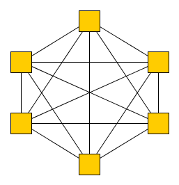
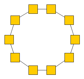
Four synthetic regular networks configurations are used: full mesh, ring, hierarchical and folded clos. In all of them, the weight of any edge is , that is, all links have cost . We will characterize the best paths in these networks, which are the paths that should be computed by a path selection algorithm.
In full mesh and ring networks all nodes are origin and destination of traffic (therefore ), see section 5. A -node full mesh is a clique (as illustrated in Figure 1(a)). Between any two distinct nodes, there is a shortest path (with cost 1) and paths of cost 2. These are the best paths, leading to a set with best paths. In a ring network each node has degree 2 and there are two (disjoint) simple paths to reach any other node (see Figure 1(b)). The set of best paths is the set of all simple paths and has elements. In both configurations, the best paths can be aggregated into trees, each one rooted at the origin node.
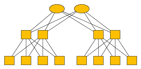
In traditional small to medium data center networks, hierarchical tree-like networks are commonly used, see Figure 2(a). In these hierarchical networks, the best paths between any two leaf nodes (the only ones that belong to ) are the shortest ones and there are such paths, where is the minimum number of levels that must be climbed to reach the destination node (all these paths are valley-free) 111A valley-free path in this context can be seen as a path that “climbs and descends only once”..
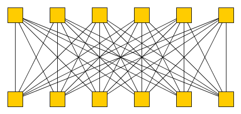
A folded clos network is defined by two distinct layers, forming a bipartite graph, where each node of the lower layer (which corresponds to the set ) is directly connected to every node of the upper layer. Figure 2(b) presents a folded clos network with the same number of nodes in each layer. For each pair of nodes of the lower layer, the best paths are the shortest paths, which are valley-free and pairwise disjoint. Their number is equal to the size of the upper layer. Therefore, in a folded clos network with nodes in each layer, there are best paths, which can be aggregated into trees. Those networks are also traditionally used in data centres and have the interesting property of maximizing path disjointness among nodes.
In the first 6 rows of Table 1 the used regular networks are characterized in terms of number of nodes, number of edges, number of best paths, and minimum number of trees to cover the best paths.
| Network | # nodes | # edges | n = | # best | min | Characterization |
|---|---|---|---|---|---|---|
| paths | # trees | (as used in this paper) | ||||
| full mesh | 12 | 66 | 12 | 726 | 12 | A clique graph |
| ring | 12 | 12 | 12 | 132 | 12 | A circular graph |
| hierarchical 2 | 14 | 24 | 8 | 152 | 8 | A two level tree-like graph |
| hierarchical 3 | 30 | 56 | 16 | 2352 | 32 | A three level tree-like graph |
| folded clos 6 | 12 | 36 | 6 | 90 | 6 | A bipartite graph |
| folded clos 12 | 24 | 144 | 12 | 792 | 12 | A bipartite graph |
| Abovenet | 15 | 44 | 15 | – | – | USA backbone |
| ATT | 35 | 68 | 35 | – | – | USA backbone |
| B4 | 12 | 19 | 12 | – | – | World wide DC backbone |
| Géant | 32 | 49 | 32 | – | – | European research backbone |
| NTT | 27 | 63 | 27 | – | – | World wide backbone |
| Sprint | 32 | 64 | 32 | – | – | World wide backbone |
| Tiscali | 30 | 76 | 30 | – | – | European backbone |
2.3 Backbone networks
Backbone networks used for testing purposes were selected using several criteria. First, only POP level network models were used since routing policies are more relevant at this level than at routers level. Besides, using the routing concretizations presented in section 5.3, several routers of the same POP can be collapsed in one logical one and ECMP (Equal Cost Multi-Path Routing) can be used to load balance traffic across several parallel links directly connecting two POPs. Second, public depicted backbones were preferred to avoid having to resort to synthesized randomized backbone topologies.
One education and research backbone (Géant), a world wide backbone (NTT Communications) and the network used in [10] were chosen since their configurations are publicly sketched. These three backbones were approximately mapped from their publicly presented diagrams. Additionally, we used four commercial ISP backbones mapped by the Rocketfuel project [20]: Abovenet, ATT, Sprint and Tiscali. Their mappings are more than 10 years old, but we still deem them representative of the most important topological characteristics of real wide area backbones.
In all those backbone networks, as the link capacities were, in general, not publicized, latency (approximately inferred from the geographic distance between the cities where the POPs are located) is used as the cost metric. This metric is closely related to latency inflation which is particularly relevant for the tested algorithms when applied to wide area backbones. To speedup computations, backbone graphs were (iteratively) shrunk by pruning them from nodes of degree 1, since these nodes do not introduce any extra diversity or path alternatives. The last 7 rows of Table 1 present the characteristics of the retained backbone networks.
The number of required paths and trees will increase when used to drive a real network routing configuration. Degree 1 nodes will be reinserted, what will increase the number of paths, but not the number of trees. Besides, provisioning of different classes of service to customers will also increase the number of paths and trees by a factor proportional to the number of different traffic classes used. However, all multi-path routing methods discussed in section 5 require the same increase in backbone state and control complexity if several service classes are used. Resource reservation for traffic classes (and therefore for different trees) is outside the scope of this paper. Anyway, in large backbones, shaping and admission control, when applied, are performed at the edge to relieve core routers of these concerns.
3 Path selection
3.1 The problem and known solutions
Given a network and a traffic matrix, to find a multi-path continuous traffic distribution that minimizes the load in all the network links is a well known optimization problem [26, 8]. This traffic distribution implicitly elects a set of paths used for routing. With several matrices, the union of the sets of paths will eventually stabilize.
Practice has shown that it is useless to select more than a small number of paths between each pair of edge nodes. In fact, the problem may be approached in the reverse direction: to speed up the optimization computation, one can a priori restrict the traffic distribution to a subset of the available paths, computed in a traffic matrix independent way, see chapter 12 of [8] for example. The common reported experience (e.g., [10]) shows that restricting the traffic distribution to a subset of paths can speedup significantly the optimization process, without any practical relevant impact in the final result optimality. In general, that subset is composed of (almost) shortest paths.
The most common approach to tackle network faults, in the context of traffic engineering, is to complete the set of paths used to optimally route traffic with backup paths. Some of the network faults may lead to non optimal traffic routing. In [22] a method is proposed to deal with this degradation. Given a set of the most common faulty scenarios, the optimal traffic distribution of the considered traffic matrix is computed for each one. Using the paths computed for each scenario, it is possible to compute a global subset of the most interesting ones. Finally, for each faulty scenario, an optimal traffic distribution is computed over the selected paths. The method requires several a priori collected pieces of information: traffic matrices and the common faulty scenarios. Both are hard to find but when the network managers have years of accumulated traffic and fault statistics with their network. Moreover, in what concerns network faults, most of them stem from old components with intermittent behaviour, software bugs and planned reconfigurations [12]. Additionally, estimating a meaningful traffic matrix is also a non trivial problem [26].
Due to these difficulties, it is common to resort to heuristic methods to a priori compute a suboptimal set of paths. A simple example, described in [19], consists in selecting, for each pair of edge nodes, a set of paths, in general just two, that includes at least two node disjoint paths whose cost stretch over the shortest ones is constrained. When it is not possible to find such a pair of paths, a shortest path and a disjoint path in terms of nodes with it are chosen. The authors use a heuristic that privileges fault-tolerance over/above traffic distribution.
SPAIN is a multi-path data center routing proposal [15] which also uses, for each pair of edge nodes, a set of paths computed independently of a traffic matrix. The algorithm has as input a network graph, a pair of edge nodes (origin and destination) and the number of paths from the origin to the destination to be computed. In each step, the algorithm starts by computing a shortest path . Then, the cost of every edge of is increased by a large number (such as the sum of the initial costs of all graph edges), to prevent its use in the next iteration if cheaper alternatives are available. The algorithm terminates when different paths have been found or the path computed in some iteration has already been selected in a previous step. This algorithm also privileges edge disjointness over/above traffic distribution but, as we will see later, it is often unable to compute paths even when they exist.
We also use a heuristic to select the best paths to support multi-path routing in a traffic matrix and fault agnostic way. However, we try to reconcile both goals: to select a set of paths deemed good for traffic distribution, as well as being able to cope with network faults. Moreover, since we also target backbone networks, we should limit latency inflation of the selected paths.
Another common traffic matrix agnostic method of computing paths for traffic load balancing is used by the two phase multi-path routing scheme, inspired by the well-known Valiant Load Balancing (VLB) [25, 11] method. To route from node to node with two phase routing, all paths formed using a shortest path from to an intermediate node , followed by a shortest path from to are used to send traffic from to .222The shortest paths from to are included because (and ) can be the intermediate node. The resulting paths provide a good solution to traffic load balance in data center networks where path latency differences are not very relevant, but are not so suited to WAN backbones spanning one or more continents. Besides, the method does not guarantee any disjointness degree among the selected paths.
3.2 Algorithm 1 – the path selection algorithm
Algorithm 1 selects a set of paths in a network (which has been characterized in section 2.1) by computing, for every pair of distinct edge nodes, , with , a set of paths from to . So, let be the pair of nodes for which we intend to compute distinct paths. Basically, those paths should be “short” and “share” few edges. The next definitions are needed to formalize these notions.
For every path in , the length of (denoted by ) is the number of its edges and the cost of () is the sum of the weights of its edges. Let be the set of simple paths from to in (which is not empty because is connected) and be the set of min-cost paths:
An optimal path is a min-cost path that has the smallest length, that is,
A set of pairwise disjoint paths (in terms of edges) is a set of paths where any edge of the graph occurs at most once. Given a set of paths, the disjointness degree of () is the maximum number of pairwise disjoint paths in or, more precisely, the maximum cardinality of the subsets of whose paths are pairwise disjoint. For example, the disjointness degree of is three because paths in are pairwise disjoint and, since there are three paths in that contain edge , only one of them can belong to a set of pairwise disjoint paths.
Sets with higher disjointness degree are usually more fault-tolerant. For this reason, the algorithm selects a set that maximizes disjointness. Among the sets with maximum disjointness degree, it computes one that minimizes “edge sharing”, “penalizing” the repeated use of the same edges. Function assigns a penalization to the (possible) use of edge in the set of paths , where denotes the number of paths in that contain :
The edge sharing in is the sum of the penalizations of the use of the graph edges in :
For the sake of illustration, let us compare the following two subsets of of cardinality 4 and disjointness degree 3:
As (because the two edges of path occur twice in ) and (because , and occur twice in ), set is considered to be better than .
Function selecPaths, presented in Figure 3, characterizes the set of paths selected in from to . Apart from the intended number of paths (), it has two more parameters, and , which allow us to restrict the length and the cost of the returned paths, as it will be explained later. If is a set and is an integer such that , let denote the set of all subsets of with elements.
In the first case, when there are at least min-cost paths, a “best” subset of of cardinality is returned. This means that the computed set satisfies the following properties:
-
•
is a subset of of cardinality : ;
-
•
has the maximum disjointness degree: ;
-
•
Among the sets with maximum disjointness degree, has the minimum edge sharing: .
In the two other cases, it is necessary to consider paths with higher cost. The selectable paths, named interesting paths, are min-cost or “near-optimal” paths. This proximity is specified by two parameters, e : limits the difference in length between a near-optimal and an optimal path, whereas controls the cost of a near-optimal path, which cannot exceed the minimum cost by a factor of . The set of the interesting paths from to is defined as follows, where denotes an optimal path from to :
If the number of interesting paths does not exceed (the second case of function selecPaths), the returned set is the set of interesting paths. So it may have less paths than what has been asked for, in which situation the network manager should be warned to take corrective actions, if possible.
When there are more than interesting paths (the last case of selecPaths and the most common one), the result set should include all min-cost paths as well as some other interesting ones, i.e., it is a union of the form , where is a “best” subset of of cardinality taking into account the fixed part . As in the first case, best means that the returned set has maximum disjointness degree and, among unions of that form of equal disjointness degree, has minimum edge sharing. It is easy to verify that both definitions of best subset can be merged, as it is shown in Figure 3.
In what concerns the implementation of the algorithm, the computation of the min-cost paths is performed efficiently by a variant of the Dijkstra algorithm [3]. However, near-optimal paths and best sets are computed by brute force methods, which use data structures or orderings so as to reduce the search space. Although the algorithm is not polynomial, it computes the result in useful time in the contexts for which it has been created (as we shall see in the next section). The number of paths between each pair of nodes () is as few as 3 or 5, for example, and the number of interesting paths is controlled by parameters and .
3.3 Algorithm 1 evaluation
In all the evaluation results presented in this paper, the algorithms were implemented in Java, using Java VM version 8, in a sequential version, without exploiting any parallelism of the supporting computer. Programs were executed in a 2.4 GHz Intel i5 CPU with 8 GB of 1600 MHz DRAM. Execution times will be referred as appropriate. Source code, input sets and results are all available from the authors.
Given a concrete network graph and the values for parameters , and , Algorithm 1 was used to compute the paths between each pair of edge nodes such that , where the order relation on nodes is the order relation on their indexes.
Synthetic regular networks.
The tests performed with these networks aimed at verifying if Algorithm 1 was able to select the best paths (defined in Section 2.2) with an adequate choice of parameters. Since all edges have cost 1, parameters and alone allow the selection of those paths, and parameter loses its significance (any value neutralizes its effect).
The best paths in a -node full mesh are selected using and . In a ring network of nodes, the best paths are selected using and . For the hierarchical networks, we used and , where denotes the level of the hierarchy. Finally, the best paths in a folded clos network with nodes in each layer are obtained with and .
Algorithm 1 computed the best paths for all regular networks. The SPAIN algorithm computed the same set of paths except with the hierarchical networks, when it is unable to select all the best paths between pairs of nodes that are connected by paths crossing the upper layer of the hierarchy. There are approximately 57% and 80% of such pairs in hierarchical networks with two and three levels, respectively.
That behaviour is due to the terminating condition of the SPAIN algorithm. In each step, a shortest path is computed and the cost of the path edges is increased by a constant large number [15], in order to prevent their use in the following iterations, until different paths have been found or the new path has already been computed in a previous iteration. By using a deterministic shortest path algorithm (such as Dijkstra’s algorithm), a path can be computed twice before all distinct shortest paths have been found, in which case the SPAIN algorithm stops prematurely and returns less than paths. The authors also recognize this limitation (in [14], section 8.3).333To see an example, let be the leftmost leaf and be the rightmost leaf of the two level hierarchical network (depicted in Figure 2(a)). The first four paths found have the form: , , and , where and are the nodes adjacent to , and are the nodes adjacent to , and and are the upper level nodes. If the edge cost increment is 24 (because there are 24 edges of cost 1 in the original network), at this moment of the execution, the edges incident upon or have weight 49 () and those incident upon or have weight 25. So, the 8 original shortest paths have the same cost again. Consequently, the fifth computed path is equal to the first one and the algorithm stops.
Computing the best paths for the three level hierarchical network, the most long computation with both algorithms, took 4722 milliseconds with Algorithm 1 and approximately 181 milliseconds with the SPAIN algorithm.
Backbone networks.
In these networks all POP nodes are considered network edge nodes. For each pair of edge nodes, Algorithm 1 chooses paths among those obeying the user provided constraints (set by and ), which form a set called the search path set or search set. Depending on the value of and the size of the search set, the computation of a best set may have a non negligible cost. Our experience shows that, although the search set can be huge, in general, very large search sets do not produce better results than smaller ones. Therefore, we developed a new version of the algorithm (Algorithm 1’), which allows for an extra parameter: an upper threshold for the size of the search set.
At runtime, for each pair, Algorithm 1’ starts by computing the search set with the given values for and . When its size is over the user provided threshold, the values of and are automatically adjusted to shrink the search set. Conversely, when the size of the search set is below and there are more paths, and are enlarged. Moreover, after selecting a best set (possibly with paths), if its disjointness degree is one, an extra fully disjoint path is added unless it does not exist. To compute this extra path the values of and are ignored. All those situations are flagged and logged.
Apart from selecting the set of paths, Algorithm 1’ also computes several characteristics of the selected sets (see below). Therefore, it is possible to run the algorithm using an increasing sequence of thresholds (e.g., 100, 150, 200, 250, …). As soon as there are no differences in the number of selected paths and in the disjointness degrees, and the differences in the average path length and cost are below a certain bound (e.g., 1%), there is no need to augment the threshold. The highest used thresholds are presented in Table 4 and varied from 100, for the most simple network (B4), and 350, for the most complex ones (ATT and Sprint).
Table 2 presents an overview of the computed results for each backbone with , , , and the mentioned thresholds. The value is often referred to as adequate for a backbone, since greater values do not allow very significant improvements in traffic distribution optimality (see for example [8, 10]). The first four columns of the table characterize the input network. The next three columns present the total number of paths computed and the averages of hop and latency stretches of these paths (an average of averages). Latency stretch is expressed in milliseconds in the same referential used to characterize link costs. The following three columns specify the percentage of pairs for which the computed set of paths has disjointness degree 1, 2, or at least 3. Finally, the last column contains the number of pairs for which Algorithm 1’ computed less than paths although they existed in the network.
The need to resize a search set was quite common and the adjustments were automatically performed as explained above. Whenever the algorithm found less than paths, there were not paths between the two nodes in the network. This happened with 3 pairs in the Géant backbone and with 14 in the ATT backbone. In all other cases the algorithm found paths. Reflecting this, the last column of the table only has 0’s.
| Network | # | # | # | # total | Average | Average | % pairs whose sets have | # pairs | ||
|---|---|---|---|---|---|---|---|---|---|---|
| nodes | edges | pairs | selected | hop | latency | disjointness degree | w/ | |||
| paths | stretch | stretch | 1 | 2 | 3 or 4 | paths | ||||
| Abovenet | 15 | 30 | 105 | 420 | 1.09 | 4.92 | 0 | 57.1 | 42.9 | 0 |
| ATT | 35 | 68 | 595 | 2366 | 1.21 | 5.00 | 16.1 | 61.7 | 22.2 | 0 |
| B4 | 12 | 19 | 66 | 264 | 1.28 | 12.9 | 0 | 87.9 | 12.1 | 0 |
| Géant | 32 | 49 | 496 | 1991 | 1.75 | 8.49 | 0 | 89.5 | 10.5 | 0 |
| NTT | 27 | 63 | 351 | 1404 | 1.04 | 11.15 | 0 | 67.2 | 32.8 | 0 |
| Sprint | 32 | 64 | 496 | 1984 | 1.25 | 6.49 | 0 | 66.1 | 33.9 | 0 |
| Tiscali | 30 | 76 | 435 | 1740 | 0.81 | 1.69 | 0 | 53.1 | 46.9 | 0 |
Node pairs for which no two fully disjoint paths were computed are rare. In the ATT backbone, after removing all degree 1 POPs, there are 3 POPs in Florida connected to the rest of the backbone by only one link, from Orlando to Atlanta. So, the 96 sets of paths that need to cross that link have disjointness degree 1. This characteristic of the network cannot be corrected since we are using the topologies made available by the Rocketfuel project, which may not represent the physical network configuration. Therefore, we only consider as worth noting situations where a 5th path was added to the 4 initially selected to ensure disjointness. This occurred for 13 pairs in the Géant backbone and for 10 in the ATT.
Algorithm 1’ is aimed at selecting paths (between a pair of nodes) that respect certain constraints relevant to their quality (set by and ). Among the eligible paths, it selects a subset that maximizes edge disjointness. It is therefore interesting to compare its results with those of a greedy algorithm that only maximizes one of these facets. For that purpose we chose again the SPAIN algorithm, whose results for the same backbones are presented in Table 3. Recall that the SPAIN algorithm mostly prioritizes edge disjointness and sometimes it is unable to find paths, even when they exist. The last column of Table 3 records those cases, which were quite frequent.
| Network | # | # | # | # total | Average | Average | % pairs whose sets have | # pairs | ||
|---|---|---|---|---|---|---|---|---|---|---|
| nodes | edges | pairs | selected | hop | latency | disjointness degree | w/ | |||
| paths | stretch | stretch | 1 | 2 | 3 or 4 | paths | ||||
| Abovenet | 15 | 30 | 105 | 385 | 0.98 | 4.87 | 0 | 57.1 | 42.9 | 22 |
| ATT | 35 | 68 | 595 | 2231 | 1.27 | 5.39 | 16.1 | 61.0 | 22.9 | 91 |
| B4 | 12 | 19 | 66 | 227 | 1.13 | 13.86 | 0 | 78.8 | 21.2 | 21 |
| Géant | 32 | 49 | 496 | 1796 | 2.30 | 8.64 | 0 | 84.3 | 15.7 | 107 |
| NTT | 27 | 63 | 351 | 1321 | 1.11 | 9.85 | 0 | 65.8 | 34.2 | 43 |
| Sprint | 32 | 64 | 496 | 1878 | 1.49 | 8.42 | 0 | 64.7 | 35.3 | 74 |
| Tiscali | 30 | 76 | 435 | 1557 | 0.83 | 1.68 | 0 | 51.8 | 48.2 | 140 |
The results show that Algorithm 1’ computed (or ) paths in all cases, as long as they existed, whereas the SPAIN algorithm did not achieve the main goal frequently, for all backbones. There is no remedy for this problem, which becomes more serious with higher values of . In spite of the SPAIN algorithm privileging edge disjointness, the results show that it only covers a higher number of faults in a relatively low percentage of pairs.
This trend is understandable and expected. We carried out several experiments with these networks, using the same values of and while changing the value of . Increasing , enlarges the search set, what often resulted, not only in bigger disjointness degrees, but also in greater cost and hop stretches. This also illustrates the flexibility Algorithm 1 provides.
Finally, Table 4 presents the thresholds used, the total execution time required by Algorithm 1’ to compute all paths, as well as the average per pair of nodes. As the time spent with each pair is highly variable, even with search sets of similar size, the table also contains the worst case, i.e., the maximum execution time for a single pair. Each pair computation being independent, the program can be easily speedup by parallelization. By contrast, the SPAIN algorithm required 617 milliseconds to compute all sets of paths for the ATT backbone, which turned out to be its more demanding network.
| Network | # pairs | Threshold | Execution time | ||
| all pairs | average per pair | worst pair | |||
| Abovenet | 105 | 150 | 8.50 | 0.081 | 0.692 |
| ATT | 595 | 350 | 372 | 0.625 | 32.495 |
| B4 | 66 | 100 | 1.46 | 0.022 | 0.194 |
| Géant | 496 | 200 | 67.7 | 0.136 | 5.384 |
| NTT | 351 | 250 | 24.3 | 0.068 | 2.102 |
| Sprint | 496 | 350 | 1240 | 2.50 | 43.618 |
| Tiscali | 435 | 250 | 10.6 | 0.024 | 0.539 |
3.4 Conclusions concerning the path selection algorithm
Algorithm 1 is not polynomial and, consequently, its running times are greater than those of greedy algorithms. For each pair of nodes, , it searches a set of paths connecting to that maximizes disjointness, among all such paths sets that respect user given hop and cost (or latency) stretch constraints.
Algorithm 1’ allows a quite fine-tuning of the paths from which the best set is selected, using parameters , and the threshold on the search set size, what is singular among algorithms with similar aims. Naturally, all this flexibility comes at the cost of an increase in running time. This increase has been shown as manageable and can be reduced using parallel execution. Also, recall that this algorithm is only executed off-line and not frequently. Besides, it also computes some properties of the chosen paths and dynamically corrects the most striking anomalies, caused by the user given parameters or the characteristics of the network. All in all, it allows a deeper knowledge of the network topology and a close control of the features of the computed set.
We now turn to the problem of efficiently using the computed paths to materialize concrete routing strategies in the network by aggregating them into trees.
4 Path aggregation into trees
As it is evident from the previous section, and clearly highlighted by the total number of paths computed (see Table 2), multi-path routing for traffic engineering requires the usage of a very significant number of different paths, of order . Moreover, different classes of traffic may still increase path numbers.
If one wants to avoid complex and dynamic routing algorithms in the core of the network, these paths must be mostly pre-configured, and reducing the state required to setup them (i.e., the size of the FIBs in routers) is an important goal. As it will be presented in section 5, using trees for this aggregation is one of the best solutions. Unfortunately, determining the minimum number of trees needed to cover a set of paths is an NP-hard problem.
4.1 The problem and known solutions
Given a set of simple paths in an undirected, simple and connected graph , the aggregation of paths into trees problem consists in computing a set of trees, with minimum cardinality, such that each path in is a path in some tree of . Recall that a tree is an undirected, simple and connected graph that is acyclic.444A cycle is a path with at least two nodes, where the first and the last nodes are equal and whose edges are all different. Without loss of generality, we assume that every path has at least two nodes. There is a subproblem of ours, named aggregation of paths with the same destination into trees, where all paths in have the same destination.
Deciding if a set of paths with the same destination can be aggregated into trees is an NP-complete problem [1, 14]. Therefore, both optimization problems referred to above are NP-hard and the known polynomial algorithms for solving them do not guarantee that the computed set of trees has minimum cardinality. The size of the returned set is the main metric to evaluate their quality.
The subproblem of aggregating paths with the same destination has been studied in the context of computing MPLS LSPs m-t-p. In [19] it is formulated as a 0–1 integer linear programming problem. A greedy algorithm is proposed in [1], which basically aggregates paths (and trees) in decreasing order of the length of their longest “common suffixes”.
Although the most general problem could be tackled with those algorithms, the final number of trees would be far from a reduced one. In general, has paths for each pair , with . Thus, , where . Partitioning paths in by the destination node would give rise to aggregation problems with the same destination and, for each one, the minimum number of computed trees would be because each of the paths with the same origin (and destination) would have to be covered by a different tree. Therefore, the final total number of trees would be at least , repetitions being not expected. This strategy will be dubbed strategy LSPs m-t-p in section 4.3.
To simplify the discussion, let us consider that a path (with ) induces the undirected graph , where is the set of nodes and is the set of edges, i.e., has the nodes and the edges in . Let also be an acyclic subgraph of and . is said to contain or cover if , and is aggregable into if is an acyclic graph. The insertion or aggregation of into transforms into the graph .
In the context of system SPAIN [14, 15], whose goals are similar to ours, Mudigonda et al. developed two randomized algorithms for aggregating paths into acyclic subgraphs (not necessarily connected). Due to their randomized nature, both algorithms must be executed several times, being returned a computed set of subgraphs with minimum size.
The first algorithm is quite simple [14, 15]. Initially, the set of subgraphs is empty. Set is traversed randomly and each of its paths, , is treated sequentially, by testing if it is covered by some subgraph in . If that is the case, is skipped; otherwise, is traversed again, in a random order, up to find a subgraph into which can be aggregated and is inserted into . When no such subgraph is found, graph becomes a new member of .
The second algorithm [14] is much more complex and its full description is outside the scope of this paper. Essentially, the algorithm has two phases. In the first one, is partitioned by the path destination node and each subproblem is solved by a reduction to the vertex colouring problem. Since the union of all computed sets (which is a solution of the original problem) can have a large number of subgraphs, the second phase tries to merge subgraphs in order to reduce the size of the returned set. The motivation presented by the authors to design this algorithm is the parallel execution of the first phase (due to the independence of the subproblems). However, the paper does not contain any comparison of both algorithms from the point of view of performance or the quality of the solutions. For this reason, our experiments include only the first algorithm whose implementation is simpler.
4.2 Algorithm 2 – the path aggregation algorithm
Algorithm 2 aggregates paths into trees in a deterministic way. Starting from an empty set of trees, paths are successively aggregated into the current trees, creating a new tree only when their insertion into any existing tree would result in a cyclic or disconnected graph. The prime difference towards the similar algorithms presented above is that “pairs of compatible paths” are first inserted in a specific order and into specific trees.
With some abuse of notation, a set with two distinct paths is called a pair, , in spite of the order irrelevance. Recall that: the input set, , is a set of paths in a graph ; denotes the graph induced by a path ; and a tree of is a connected and acyclic subgraph of (defined by ).
The key notion of “compatibility” is defined over two paths, over a path and a tree, and over a pair of paths and a tree. Compatibility of two paths will be used to specify the order in which paths pairs are processed. The two other compatibility types will be used to identify the tree where a path or a pair of paths is inserted, when there are several alternatives.
By definition, the compatibility degree of a pair of paths is , if graph is cyclic; otherwise, it is , the number of common nodes. The compatibility degree of a path and a tree is defined in an identical way: it is if graph is cyclic; and , otherwise. The compatibility degree of a pair of paths and a tree is: if graph is cyclic; and , otherwise.
Two paths (respect., a path and a tree, or a pair of paths and a tree) are said to be compatible if their compatibility degree — denoted by — is positive. Note that two paths (respect., a path and a tree) without common nodes are not compatible, because the union of the corresponding graphs is disconnected. However, a pair of paths can be compatible with a tree even if one of the paths does not share any node with the tree (providing the other does).
The following properties, which justify the operations on compatible entities, are easy to verify:
-
•
If is a pair of compatible paths, the graph created with is a tree.
-
•
If a path and a tree are compatible, the insertion of into , which transforms into the graph , yields a tree.
-
•
If is a pair of compatible paths, is a tree, and and are compatible, the insertion of into , which transforms into the graph , yields a tree.
The algorithm comprises four main phases: (i) generation of all pairs of compatible paths; (ii) aggregation of pairs of compatible paths; (iii) generation of all single paths, which are the paths in that were not treated in the previous step (because, for instance, they are incompatible with any other path); (iv) aggregation of single paths.
In the first phase, the compatibility degrees of all pairs of paths in are computed. Compatible pairs will be processed in the second phase, in an order that follows three criteria: first, in decreasing compatibility degree of the pair; second, in decreasing “aggregation potential” of the pair in ; and, in case of equal compatibility degrees and aggregation potentials, in decreasing length of the pair (which is the sum of the lengths of both paths).
The first criterion aims at privileging the pairs whose aggregation is more “natural”, i.e., those whose aggregation result differs less from each of the paths. The “aggregation potential” gives priority to pairs of paths that share many common nodes with their compatible paths. Formally, the aggregation potential of a path in set is the sum of the compatibility degrees of all compatible pairs of encompassing :
The aggregation potential of a pair of paths in set is the sum of the aggregation potentials of and in :
Finally, the goal of the third criterion is to treat the longest paths as soon as possible, when there are more alternatives, deferring those that, in principle, are easier to aggregate.
In the aggregation phase of the compatible pairs of paths, each pair is processed in the order introduced above, until there are no more pairs left. The algorithm starts by verifying, for each path of the pair, whether it is covered by some of the existing trees. Three cases can arise. In the first one, both paths are contained in trees (possibly different) and the processing of the pair ends. In the second case, none of the paths is contained in a tree. If there is some tree compatible with the pair, the pair is inserted into an existing tree (specifyed below); otherwise, a new tree is created with the pair. In the third case, one of the paths is contained in some tree and the other (which will be designated by ) is not covered by any tree. If is compatible with , it is aggregated into ; if is not compatible with but there is some tree compatible with , is inserted into an existing tree (see below); otherwise, no tree is compatible with , so is ignored and its aggregation is postponed until the fourth phase.
In the third phase, paths that have not been treated yet are sorted in decreasing order of length, to be processed in the last step. The processing of a singular path also starts by searching a tree that covers it. If there is any, nothing more is done. Otherwise, if is compatible with some tree, is inserted into an existing tree; when is incompatible with all available trees, tree is created and added into the result set.
The search for a compatible tree with a path or a pair of paths returns, in case of success, the tree where will be inserted. That tree is, among all those compatible with , one that maximizes the compatibility degree. Thus, if is the set of all existent trees, the tree where is aggregated verifies: and .
The running time of the algorithm is , where denotes the set of nodes of network , due to the following. The compatibility degree of two entities can be computed in steps, because all nodes belong to and the length of any path cannot exceed . Therefore, the first phase is , since all pairs of paths are analysed and compatible pairs are sorted. The third phase is , due to sorting. In the two aggregation phases, all pairs of compatible paths and all single paths are processed. As the processing of each pair or single path requires time, where represents the current set of trees, the total cost of these phases is . The conclusion stems from the fact that .
In the following section we present the evaluation of the algorithm while aggregating the paths computed by the path selection algorithm.
4.3 Algorithm 2 evaluation
In this evaluation we used the sets of paths computed with Algorithms 1 and 1’, as presented in section 3.3. Once again, the tests performed with the synthetic regular networks (full mesh, ring, hierarchical and folded clos networks) were significant to assess the absolute quality of the results, since the minimum number of trees needed to cover all paths is known (recall Table 1 in section 2.2). Therefore, we can compare the results obtained with the optimal ones, in contrast to those achieved with the backbone networks, for which the optimal solutions are unknown.
Table 5 presents the most important data and results. The first columns identify the network, the number of edge nodes (n = ), the desired number of paths between each pair of nodes (), and the total number of paths to be aggregated (). For the regular networks, the minimum number of trees required to cover the paths is then shown. The next two columns contain the number of trees built by Algorithm 2 and the number of graphs computed by the first algorithm proposed for the system SPAIN (see [14, 15] and the discussion in section 4.1). The last column presents the number of trees that would be obtained by the strategy LSPs m-t-p (see again section 4.1), which corresponds to .
| Network | min | # acyclic subgraphs | LSPs | ||||
| # trees | Algorithm 2 | SPAIN | m-t-p | ||||
| full mesh | 12 | 11 | 726 | 12 | 12 | 56 | 121 |
| ring | 12 | 2 | 132 | 12 | 12 | 12 | 22 |
| hierarchical 2 | 8 | 2 or 8 | 152 | 8 | 8 | 10 | 56 |
| hierarchical 3 | 16 | 2, 8 or 32 | 2352 | 32 | 40 | 71 | 496 |
| folded clos 6 | 6 | 6 | 90 | 6 | 6 | 13 | 30 |
| folded clos 12 | 12 | 12 | 792 | 12 | 12 | 58 | 132 |
| Abovenet | 15 | 4 | 420 | — | 24 | 26 | 56 |
| ATT | 35 | 4 | 2366 | — | 54 | 65 | 136 |
| B4 | 12 | 4 | 264 | — | 20 | 20 | 44 |
| Géant | 32 | 4 | 1991 | — | 57 | 69 | 120 |
| NTT | 27 | 4 | 1404 | — | 42 | 56 | 104 |
| Sprint | 32 | 4 | 1984 | — | 52 | 68 | 124 |
| Tiscali | 30 | 4 | 1740 | — | 27 | 36 | 116 |
Being a randomized algorithm, the SPAIN algorithm was executed several times with the same set of paths. But, instead of defining the exact number of executions (also called iterations) per network, we limited its total execution time to 100 times the time required by Algorithm 2 for the same network. Table 5 has the minimum number of subgraphs computed in all iterations. Table 6 presents the execution times of Algorithm 2, the thresholds for the total execution time of the SPAIN algorithm and the number of iterations it actually performed during that time. It is worth noting that this algorithm has been implemented as described in section 4.1 and by the authors of [14, 15]. Consequently, the output is a set of acyclic graphs, not necessarily connected (what justifies the common title of the two Table 5 columns that present the results).
| Network | Algorithm 2 | SPAIN | |
| execution time | threshold | # iterations | |
| full mesh | 0.197 | 19.7 | 4384 |
| ring | 0.002 | 0.2 | 2140 |
| hierarchical 2 | 0.034 | 3.4 | 10417 |
| hierarchical 3 | 16.565 | 1656.5 | 71642 |
| folded clos 6 | 0.012 | 1.2 | 3270 |
| folded clos 12 | 0.302 | 30.2 | 2793 |
| Abovenet | 0.067 | 6.7 | 6169 |
| ATT | 2.276 | 227.6 | 14125 |
| B4 | 0.020 | 2 | 3247 |
| Géant | 1.091 | 109.1 | 7533 |
| NTT | 0.670 | 67 | 7623 |
| Sprint | 1.159 | 115.9 | 8671 |
| Tiscali | 1.885 | 188.5 | 33978 |
Results show that Algorithm 2 computes the optimal solution for almost all regular networks but the hierarchical 3 one, where the result is approximately 25% far from the minimum. In spite of the allowed running times, the SPAIN algorithm only discovered the optimal trees with the ring network. In all other cases it returned a number of graphs between 37.5% (hierarchical 2) and 383% (folded clos 12) far from the optimal. In what concerns the backbones, where optimal solutions are not known, Algorithm 2 always outperformed the SPAIN algorithm, except in the B4 case for which both returned equivalent sets. Values in the LSPs m-t-p column are always substantially higher than those obtained with the two algorithms, which indicates a lack of effectivity in that strategy when the goal is to significantly reduce the size of the FIBs in the core of the network. We will discuss in the next section how these results can be used to drive traffic routing in the network.
5 Implementing multi-path routing using trees and off-the-shelf network equipment
In the previous two sections we have presented and evaluated two algorithms intended to support multi-path routing in a backbone network.
The first algorithm allows network managers to compute a set of paths that can be used to route ingress flows to their egress nodes, using load distribution among these paths. This paves the way for offline or online optimization. We envision online optimization using a centralized controller that periodically adjusts traffic distributions. We leave for future work the study of the relation between traffic distribution optimality and the estimated accuracy of the traffic matrix and of network path availability. We anticipate that it is possible to find a reasonable solution even if the central controller only updates its vision of network and the traffic matrix from time to time (with a period of several minutes for example).
The second algorithm supports a scalable way of path deployment in the core of the network by the way of a reduced number of trees. In the next paragraphs we will present several alternatives for this deployment using different types of off-the-shelf equipment and simple protocols. By hypothesis, mechanisms required to implement traffic engineering must be available in each ingress node , allowing it to: H1) given the destination address of a packet flow, to know , the flow egress node; H2) given an egress node , to know paths to get there; and H3) given the paths that allow to reach , which one should be chosen for that flow (in accordance to some load distribution criteria). The availability of these mechanisms is discussed below. The way edge routers, servers or a central controller use them to establish traffic engineering policies is left for future work.
5.1 Routing with trees using MPLS and multipoint-to-point LSPs
As already mentioned in the introduction, MPLS is the most popular way to implement traffic engineering. Since the total number of different required LSPs may be very important, multipoint-to-point LSPs can be used to reduce the state in the network (see section 4). In that section we have shown that it is possible to have less state in the network by the way of leaving the restriction that each such directed acyclic graph should be rooted in the egress node and only supports traffic in the direction of the egress node. Anyway, using MPLS for traffic engineering is a known technique, and mechanisms H1), H2) and H3) are part of the available implementations.
5.2 Routing with trees using VLANs
In a network of Ethernet switches it is possible to statically parametrize in each switch a mapping from ports to VLANs [15]. Each tree, encompassing different paths, is then supported by a different VLAN. With this solution, the selection of a path to a destination switch (egress node) is implemented by choosing the corresponding VLAN tag. Routing is then performed using VLAN restricted flooding and filtering on the basis of the destination address.
This solution has been proposed and tested in a data center network scenario [15] and the required flow distribution mechanisms (H1, H2 and H3) were implemented by the servers Ethernet drivers. These drivers implemented a sort of static mapping from server MAC addresses to switch addresses and VLAN tags, as well as protocols to detect path availability and the speedup of filtering mechanisms in the network switches. The authors of the proposal used a uniform random distribution of the flows among the different available paths (or trees) and left for future work the study of the impact of the usage of non uniform distributions.
5.3 Routing with trees using longest-prefix matching routing
It is also possible to implement multi-path routing by the way of several rooted trees using hierarchical IP addresses and Longest-Prefix Matching. For this purpose, it is possible to parametrize routers, using remotely setup static routing, in the following way. Each tree is associated with an IP prefix (an interval of addresses which size is a power of 2). The intersection of all the intervals must be empty. Then, each is partitioned in as many sub prefixes as the root has descendants in this tree, and each sub prefix of is associated with a different descendant node. This process continues recursively up to the leaf nodes of the tree. In each node, but the root, the parent prefix is associated with all the interfaces leading to the parent node, and each sub prefix is associated with all the interfaces leading to the descendant associated with each sub prefix. Finally, each node receives an address in its (sub)prefix that it keeps for itself. Any node will have as many addresses as trees it belongs to [24]. The same applies for the number of static routes associated with its interfaces. Each router can also have an IP address, in a different prefix, routed by a shortest-path protocol to guarantee a direct control channel and a fallback path.
The choice of the path a packet will follow is performed by choosing the address of the destination router in the tree encompassing the chosen path. This packet address destination transformation can be performed by the way of tunnels to preserve the original destination address. Using LISP [4] to support routing in this scenario is a standardized way of implementing the tunnels, directly providing interfaces to mechanisms H1, H2 and H3.
5.4 Routing with trees using OpenFlow
According to several authors (e.g., [17]) and as already mentioned in the introduction, a vision where, for each different micro flow, state is installed in the network is not scalable for intra-AS networking or for intra data center routing. Also, recent proposals related to the usage of the SDN approach in the wide area intra-AS routing (e.g., [9, 10]) rely on the usage of tunnels and logically centralized controllers that perform path selection decisions based on a global view of the network configuration and status.
Routing with trees, and their implementations based on VLANs or on IP-based longest-prefix matching routing, can also be implemented in the core of the network using OpenFlow. Their usage requires the evaluation of a tradeoff between routing space and forwarding complexity.
6 Discussion and conclusions
Provider backbone networks need flexible and adaptable mechanisms to support traffic engineering with varying demands and promptly adaptation to network faults. Currently, these goals are fulfilled using expensive and sophisticated equipments that run distributed algorithms and implement dynamic routing in the core of the network (e.g., MPLS tunnels and dynamic trunk rerouting) as well as a certain degree of over provisioning the network.
One of the most long standing principles of complex systems design, the end-to-end argument, argues for a core as simple as possible and relegates to the edge most of the complexity and adaptation to varying requirements. Applied to routing, this design rule would avoid as much as possible complexity in the core and, in particular, avoid the implementation of the support of diversity and adaptation to varying requirements in the core, as currently is partially the rule. This line of thinking is aligned with proposals like those presented in [2, 15, 22] and is also partially aligned with the SDN proposal [13, 5, 17].
Our quest for a simpler support for traffic engineering without sacrificing optimality and adaptability to demand variations and network faults lead us to envision a simple core, able to a priori provide as many paths as required by the edge to adapt traffic to variable requirements, as proposed in [15] for example, or to network faults as proposed in [22] for example.
To pre-compute these path sets we developed Algorithm 1 for path selection in a fault and demand agnostic way. Its evaluation, in the context of several provider backbones, showed that it is feasible to pre-compute a set of paths able to support continuous connectivity and providing sufficient diversity to support traffic rerouting in face of a set faults. We insure that these sets support at least one faulty link, what seems compatible with current practice if there is no lower level implied correlation among faults, like several links sharing the same fiber or the same conduct. Altough the full evaluation of the ability of the computed path sets to support flexible adaptation to traffic variability is left for future work, many authors have referred that using 3 to 5 different paths between each pair of edge nodes is sufficient to support almost optimal traffic load balancing when path link disjunction is maximized as we also do. Algorithm 1 is more complex than other alternatives but, as we have shown, it always finds the demanded number of paths if they are available in the network, and the computed set is also able to support at least one link fault if the network also is.
The total number of computed paths is naturally very important and their continuous availability requires many FIB entries in core routers. To address this problem we have developed Algorithm 2, for aggregating paths into trees, with better results than the previously proposed algorithms with the same goal. Finally, we have shown that off-the-shelf equipment supporting simple protocols may be used to implement routing with a reduced number of trees, what shows that simplicity can be achieved by using only trivially available protocols and their most common and unsophisticated implementations.
In networks where providers control not only the network but also customer demands, like in private inter data center networks, an architecture is emerging [10, 9, 6]: a centralized controller (or a hierarchy of several ones) receives information on traffic demands, schedules them, and adapts routing decisions to optimize network usage. The ultimate goal being to avoid as much as possible network over provision. This kind of control architecture can only be partially adopted in a provider network since the provider has almost no control over customer demands. However, we think that it is possible to adopt a similar architecture. To make it real, there are several problems that must be addressed: how can the central controller timely know current customer demands and influence them? how can the central controller dynamically adapt routing to demands? what is the cost versus accuracy needed to close the loop on customer demands awareness and optimality of traffic engineering? and so on.
We intend to tackle these problems in our future work. The algorithms introduced in this paper are central to the conception of that architecture, since they permit a network design where in fact all complexity is concentrated in edge routers and the controller, while the core can be simple and based on off-the-shelf equipment and off-the-shelf simple protocols.
References
- [1] S. Bhatnagar, S. Ganguly, and B. Nath. Label space reduction in multipoint-to-point LSPs for traffic engineering. Universal Multiservice Networks, 2002. ECUMN 2002. 2nd European Conference on, pages 29–35, 2002.
- [2] M. Caesar, M. Casado, T. Koponen, J. Rexford, and S. Shenker. Dynamic route recomputation considered harmful. SIGCOMM Comput. Commun. Rev., 40(2):66–71, Apr. 2010.
- [3] E. Dijkstra. A note on two problems in connection with graphs. Numerische Mathematik, 1(269-270):6, 1959.
- [4] D. Farinacci, V. Fuller, D. Meyer, and D. Lewis. The Locator/ID Separation Protocol (LISP). RFC 6830 (Experimental), IETF, Jan. 2013.
- [5] N. Feamster, J. Rexford, and E. Zegura. The road to sdn. Queue, 11(12):20:20–20:40, Dec. 2013.
- [6] A. Ghosh, S. Ha, E. Crabbe, and J. Rexford. Scalable multi-class traffic management in data center backbone networks. Selected Areas in Communications, IEEE Journal on, 31(12):2673–2684, December 2013.
- [7] A. Greenberg, J. R. Hamilton, N. Jain, S. Kandula, C. Kim, P. Lahiri, D. A. Maltz, P. Patel, and S. Sengupta. Vl2: a scalable and flexible data center network. In Proceedings of the ACM SIGCOMM 2009 conference on Data communication, SIGCOMM ’09, pages 51–62, New York, NY, USA, 2009. ACM.
- [8] O. M. Heckmann. The Competitive Internet Service Provider. Wiley Series in Communications Networking & Distributed Systems. Wiley-Interscience, Chichester, UK, 1 edition, April 2006.
- [9] C.-Y. Hong, S. Kandula, R. Mahajan, M. Zhang, V. Gill, M. Nanduri, and R. Wattenhofer. Achieving high utilization with software-driven wan. In Proceedings of the ACM SIGCOMM 2013 Conference on SIGCOMM, SIGCOMM ’13, pages 15–26, New York, NY, USA, 2013. ACM.
- [10] S. Jain, A. Kumar, S. Mandal, J. Ong, L. Poutievski, A. Singh, S. Venkata, J. Wanderer, J. Zhou, M. Zhu, J. Zolla, U. Hölzle, S. Stuart, and A. Vahdat. B4: Experience with a globally-deployed software defined wan. SIGCOMM Comput. Commun. Rev., 43(4):3–14, Aug. 2013.
- [11] M. Kodialam, T. V. Lakshman, and S. Sengupta. Traffic-oblivious routing in the hose model. IEEE/ACM Trans. Netw., 19(3):774–787, jun 2011.
- [12] A. Markopoulou, G. Iannaccone, C.-N. C. S. Bhattacharyya, Y. Ganjali, and C. Diot. Characterization of failures in an operational ip backbone network. IEEE/ACM Transactions on Networks, 16(4):749–762, 2008.
- [13] N. McKeown, T. Anderson, H. Balakrishnan, G. Parulkar, L. Peterson, J. Rexford, S. Shenker, and J. Turner. Openflow: Enabling innovation in campus networks. SIGCOMM Comput. Commun. Rev., 38(2):69–74, Mar. 2008.
- [14] J. Mudigonda, P. Yalagandula, M. Al-Fares, and J. Mogul. Spain: Design and algorithms for constructing large data-center ethernets from commodity switches. Technical report, Tech. Rep. HPL-2009-241, HP Labs, 2009.
- [15] J. Mudigonda, P. Yalagandula, M. Al-Fares, and J. Mogul. Spain: Cots data-center ethernet for multipathing over arbitrary topologies. In Proceedings of the 7th USENIX conference on Networked systems design and implementation, pages 18–18. USENIX Association, 2010.
- [16] A. Pathak, M. Zhang, Y. C. Hu, R. Mahajan, and D. Maltz. Latency inflation with mpls-based traffic engineering. In Proceedings of the 2011 ACM SIGCOMM Conference on Internet Measurement Conference, IMC ’11, pages 463–472, New York, NY, USA, 2011. ACM.
- [17] B. Raghavan, M. Casado, T. Koponen, S. Ratnasamy, A. Ghodsi, and S. Shenker. Software-defined internet architecture: Decoupling architecture from infrastructure. In Proceedings of the 11th ACM Workshop on Hot Topics in Networks, HotNets-XI, pages 43–48, New York, NY, USA, 2012. ACM.
- [18] E. Rosen, A. Viswanathan, and R. Callon. Multiprotocol label switching architecture. IETF, RFC 3031, 2001.
- [19] H. Saito, Y. Miyao, and M. Yoshida. Traffic engineering using multiple multipoint-to-point lsps. In INFOCOM 2000. Nineteenth Annual Joint Conference of the IEEE Computer and Communications Societies. Proceedings. IEEE, volume 2, pages 894 –901 vol.2, 2000.
- [20] N. Spring, R. Mahajan, and T. Anderson. Quantifying the causes of path inflation. In Proceedings of the ACM SIGCOMM 2003 conference on Data communication, SIGCOMM ’2003. ACM, 2003.
- [21] B. Stephens, A. Cox, W. Felter, C. Dixon, and J. Carter. Past: Scalable ethernet for data centers. In Proceedings of the 8th International Conference on Emerging Networking Experiments and Technologies, CoNEXT ’12, pages 49–60, New York, NY, USA, 2012. ACM.
- [22] M. Suchara, D. Xu, R. Doverspike, D. Johnson, and J. Rexford. Network architecture for joint failure recovery and traffic engineering. SIGMETRICS Performance Evaluation Review-Measurement and Evaluation, 39(1):97, 2011.
- [23] C. Systems. Cisco visual networking index (vni). http://www.cisco.com/c/en/us/solutions/service-provider/visual-networking-index-vni/index.html.
- [24] P. F. Tsuchiya. Efficient and robust policy routing using multiple hierarchical addresses. In Proceedings of the conference on Communications architecture & protocols, SIGCOMM ’91, pages 53–65, New York, NY, USA, 1991. ACM.
- [25] L. G. Valiant. A scheme for fast parallel communication. SIAM journal on computing, 11(2):350–361, 1982.
- [26] N. Wang, K. H. Ho, G. Pavlou, and M. Howarth. An overview of routing optimization for internet traffic engineering. IEEE Communications Surveys and Tutorials, 10(1):36–56, 2008.