Applications of spectral theory to special functions

Abstract.

Many special functions are eigenfunctions to explicit operators, such as difference and differential operators, which is in particular true for the special functions occurring in the Askey-scheme, its $q$-analogue and extensions. The study of the spectral properties of such operators leads to explicit information for the corresponding special functions. We discuss several instances of this application, involving orthogonal polynomials and their matrix-valued analogues.

Preamble

We use standard notation for hypergeometric series, basic hypergeometric series (also known as $q$-hypergeometric series) and special functions following standard references, such as e.g. Andrews, Askey and Roy [5], Gasper and Rahman [29], Ismail [47], Koekoek and Swarttouw [54], [55], Szegő [93], Temme [94]. There is an abundance of references, and apart from the references in the books in the bibliography, the review paper by Damanik, Pushnitski and Simon [19] contains many references. The appendix discusses the spectral theorem, and references are given there. All measures discussed are Borel measures on the real line, and we denote the $\sigma$-algebra of Borel sets on $\mathbb{R}$ by $\mathscr{B}$. Furthermore, $\mathbb{N}=\{0,1,2,\cdots\}$. All the results in these notes have appeared in the literature.

1. Introduction

Spectral decompositions of self-adjoint operators on Hilbert spaces can at least be traced back to the work of Fredholm on the solutions of integral equations. The study of Sturm-Liouville differential operators was a great impetus for the development of spectral analysis, see e.g. [22]. For some explicit Sturm-Liouville type differential operators there is a link to well-known special functions, such as e.g. Jacobi polynomials, which shows the close connection between special functions and spectral theory. At the moment, this is for instance an important ingredient in the study of so-called exceptional orthogonal polynomials, see e.g. [24].

Spectral theory is, loosely speaking, essentially a study of the eigenvalues, or spectral data, of a suitable operator, and to determine such an operator completely in terms of its eigenvalues. For a self-adjoint matrix this means that we look for its eigenvalues, which are real in this case, and the corresponding eigenspaces, which are orthogonal in this case. So we can write the self-adjoint matrix as a sum of multiplication and projection operators, and this is the most basic form of the spectral theorem for self-adjoint operators. We recall the spectral theorem in its most general form in Appendix A.

The application to differential operators, and also to various developments in physics, such as quantum mechanics, is still very important. Through this application, there have been many developments for special functions. One of the classical applications is to study the second order differential operator

$$D^{\alpha,\beta}=(1-x^{2})\frac{d^{2}}{dx^{2}}+\bigl{(}\beta-\alpha-(\alpha+\beta+2)x\bigr{)}\frac{d}{dx}$$

on the weighted $L^{2}(w^{\alpha,\beta})$ space for the weight $w^{\alpha,\beta}(x)=C(1-x)^{\alpha}(1+x)^{\beta}$ on $[-1,1]$ for a suitable normalisation constant $C$. Then $D^{\alpha,\beta}$ can be understood as an unbounded self-adjoint operator with compact resolvent. The spectral measure is then given by projections on the orthonormal Jacobi polynomials, which are eigenfunctions of $D^{\alpha,\beta}$. Similarly, the differential operator can also be studied on $[1,\infty)$ with respect to a suitable weight, and then its spectral decomposition leads to the Jacobi-function transform, see e.g. [23, Ch. XIII], [69] and references.

Another classical application of spectral analysis is a proof of Favard’s theorem, see Corollary 3.7, stating that polynomials satisfying a suitable three-term recurrence relation, are orthogonal polynomials. This follows from studying a so-called Jacobi operator on the Hilbert space $\ell^{2}(\mathbb{N})$ of square summable sequences. The spectral analysis of such a Jacobi operator is closely related to the moment problem, and this link can be found at several places in the literature such as e.g. [20], [23], [57], [87], [88], [89]. The Haussdorf moment problem, i.e. on a finite interval, played an important role in the development of functional analysis, notably the development of functionals and related theorems, see [79, §I.3].

One particular application is to have other explicit operators, e.g. differential operators or difference operators, realised as Jacobi operators and next use this connection to obtain results for these explicit operators. In Section 6 we give a couple of examples, including the original (as far as we are aware) motivating example of the Schrödinger operator with Morse potential due to the chemist Broad, see references in Section 6.1.

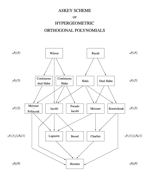
Figure 1. The Askey scheme as in [54].

As is well-known the Askey scheme of hypergeometric orthogonal polynomials and its $q$-analogue, see e.g. [54], [55], and initially observed by Askey in [9, Appendix], see also the first Askey-scheme in Labelle [74] –drawn by hand–, consists of those polynomials which are also eigenfunctions to a second-order operator, which can be a differential operator, a difference operator or a $q$-difference operator of some kind. See Figures 1 and 2, taken from Koekoek, Lesky, Swarttouw [54] for the current state of affairs. Naturally, many of these operators, like the differential operator for the Jacobi polynomials, have been studied in detail. This is in particular valid for the operators occurring in the Askey-scheme. For the other operators, especially the difference operators for the orthogonal polynomials in the $q$-analogue of the Askey scheme corresponding to indeterminate moment problems, see [15]. On the other hand, it is natural to extend the ($q$-)Askey-scheme to include also integral transforms with kernels in terms of (basic) hypergeometric series, such as the Hankel, Jacobi, Wilson transform, and its $q$-analogues and to study these transforms and their properties from a spectral analytic point of view using the associated operators. We refer to the schemes [65, Fig. 1.1, 1.2] remarking that in the meantime [65, Fig. 1.1] has been vastly extended to include the Wilson function transform by Groenevelt [32], and various transformations that can be obtained as limiting cases. In the terminology of Grünbaum and coworkers, all the instances of the ($q$-)Askey-scheme are examples of the bispectral property. This means that the polynomials are eigenfunctions to a three-term recurrence operators (acting in the degree) and at the same time are eigenfunctions of a suitable second order differential or difference operator in the variable. In particular, all these instances give rise to bispectral families of special functions.

Figure 2. The $q$-Askey scheme as in [54].

Motivated by one of the second order $q$-difference operators arising in the $q$-analogue of the Askey-scheme, we discuss the spectral analysis of three-term recurrence operators on $\ell^{2}(\mathbb{Z})$ in Section 2. We apply the spectral theorem to a particular example and we obtain a set of orthogonality measures for the continuous $q^{-1}$-Hermite polynomials. Here we follow the convention $0<q<1$, so that $q^{-1}>1$. These measures turn out to be N-extremal, where N stands for Nevanlinna. This result is originally obtained by Ismail and Masson [51], and this proof is due to Christiansen and the author [17] as a special case of results for the symmetric Al-Salam–Chihara polynomials for $q>1$. This is partly based on [57, §4]. Similar ideas have been used in e.g. [16], [40], to study other moment problems and related orthogonal polynomials.

In Section 3 we briefly recall the relation between three-term recurrence operators and orthogonal polynomials. This is a well known subject in the literature, and there are several books and review papers on this subject, e.g. [2], [14], [23], [76], [87, Ch. 16], [88], [89], [92]. We base ourselves on [57], and we extend this approach to the case of matrix-valued orthogonal polynomials and block Jacobi operators. The spectral approach is essentially due to M.G. Kreĭn [72], [73], whose great mathematical legacy is discussed in [1]. We discuss briefly a rather general example of arbitrary size. In Section 5 we discuss some of the assumptions made in the Section 4. Here we make also use of previous lecture series by Berg [12] and Durán and López-Rodríguez [26], but also [6], [31], [72], [73].

In Section 6 we show how realisations of explicit operators, such as differential operators, as recurrence operators can be used to study the spectral theory. This gives rise to relations between the spectral decomposition of such an operator and the related orthogonal polynomials. In the physics literature such a method is known as the $J$-matrix method, and there is a vast literature of physics applications, see e.g. references to work of Al-Haidari, Bahlouli, Bender, Dunne, Yamani and others in [48]. The first example of Section 6 is the study of the Schrödinger operator with a Morse potential, originally due to Broad [13], see also [21]. The second example of Section 6 is in the same vein, and due to Ismail and the author [48]. This case has recently been generalised by Genest et al. [30] to include more parameters and to cover the full family of Wilson polynomials. Moroever, in [30] a link to the Bannai-Ito algebra is established. The last example of Section 6 leads to a more general family of matrix-valued orthogonal polynomials for operators which have a realisation as a $5$-term recurrence operator. We then discuss an example of such a case, extending the second example of Section 6. We apply this approach to an explicit second order differential operator. The same realisation of suitable operators as tridiagonal operators has useful implications in e.g. representation theory, see e.g. [18], [33], [34], [37], [39], [42], [43], [58], [67], [78], [80] for the case of representation theory of the Lie algebra $\mathfrak{su}(1,1)$ and its quantum group analogue. Using explicit realisations of representations, these results have given very explicit bilinear generating functions, see e.g. [35], [68].

All the general results as well as the explicit examples have appeared in the literature before. There are many other references available in the literature, and apart from the books –and the references mentioned there– mentioned in the bibliography, one can especially consult the references in [19], where a list of more than 200 references can be found. In particular, there are many papers available that generalise known results in the general theory of orthogonal polynomials to the matrix-valued orthogonal polynomial case, and we refer to the references to work by Berg, Cantero, Castro, Durán, Geronimo, Grünbaum, de la Iglesia, Lopéz-Rodríguez, Marcellán, Pacharoni, Tirao, Van Assche, etc. to the references in [19].

Let us note that in these notes the emphasis is on explicit operators related to explicit sets of special functions, so that information on these special functions is obtained from the spectral analysis. On the other hand, there are also many results on the spectral analysis of more general classes of operators. For this subject one can consult Simon’s book [90] and the extensive list of references given there.

It may happen that a differential or difference operator with suitable eigenfunctions in terms of well-known special functions cannot be suitably realised as a three-term recurrence operator on a Hilbert space such as $\ell^{2}(\mathbb{Z})$ or $\ell^{2}(\mathbb{N})$. It can then be very useful to look for a larger Hilbert space, and an extension of the operator to the larger Hilbert space. This is different from the extension of a Hilbert space in order to find self-adjoint extensions. Then one needs to find a way of obtaining the extended Hilbert space and the extension of the operator. This is usually governed by the interpretation of these operators and special functions in a different context, like e.g. representation theory. Examples are in e.g. [32], [36], [63], [66], [80]. This leads to extensions of the Askey and $q$-Askey scheme of Figures 1, 2 with non-polynomial function transforms arising as the spectral decomposition of suitable differential and difference operators on Hilbert spaces of functions, see e.g. Figures 1.1 and 1.2 in [65]. Figure 1.2 of [65] is still valid as an extension of the $q$-Askey scheme, but Figure 1.1 of [65] has now Groenevelt’s Wilson function transforms [32] at the top level.

Acknowledgement. Thanks to René Swarttouw and Roelof Koekoek for their version of the Askey-scheme in Figures 1 and 2. I thank the organisers of the summer school, in particular Howard Cohl, Mourad Ismail and Kasso Okoudjou, for the opportunity to give the lectures at Orthogonal Polynomials and Special Functions Summer School OPSF-S6, July 2016, University of Maryland. I also thank all the participants of OPSF-6 for their feedback. I thank Wolter Groenevelt and Luud Slagter for their input. The referees have pointed out many errors and oversights, and I thank them for their help in improving these lecture notes.

2. Three-term recurrences in $\ell^{2}(\mathbb{Z})$

In this section we discuss three-term recurrence relations on the Hilbert space $\ell^{2}(\mathbb{Z})$. We apply to this one particular example, which is motivated by a second order difference operator arising in the $q$-Askey scheme.

We consider sequence spaces and the associated Hilbert spaces as in Example A.1. For the Hilbert space $\ell^{2}(\mathbb{Z})$ with orthonormal basis $\{e_{l}\}_{l\in\mathbb{Z}}$ we consider for complex sequences $\{a_{l}\}_{l\in\mathbb{Z}}$, $\{b_{l}\}_{l\in\mathbb{Z}}$, $\{c_{l}\}_{l\in\mathbb{Z}}$ the operator

$$L\,e_{l}=a_{l}e_{l+1}+b_{l}e_{l}+c_{l}e_{l-1},\qquad l\in\mathbb{Z},$$ (2.1)

with dense domain $\mathcal{D}$ the subspace of finite linear combinations of the basis vectors.

Lemma 2.1.

$L$ extends to a bounded operator on $\ell^{2}(\mathbb{Z})$ if and only if the sequences $\{a_{l}\}_{l\in\mathbb{Z}}$, $\{b_{l}\}_{l\in\mathbb{Z}}$, $\{c_{l}\}_{l\in\mathbb{Z}}$ are bounded.

In Exercise 1 you are requested to prove Lemma 2.1.

In case $L$ is bounded, we see that $L$ acting on $v=\sum_{k\in\mathbb{Z}}v_{k}e_{k}\in\ell^{2}(\mathbb{Z})$ is given by

$$Lv=\sum_{k\in\mathbb{Z}}(a_{k-1}v_{k-1}+b_{k}v_{k}+c_{k+1}v_{k+1})\,e_{k}.$$ (2.2)

In case $L$ is not bounded, we have to interpret this in a suitable fashion, by e.g. initially allowing only for $v\in\ell^{2}(\mathbb{Z})$ with only finitely many non-zero coefficients, i.e. for $v\in\mathcal{D}$. In general we view $L$ as an operator acting on the sequence space of sequences labeled by $\mathbb{Z}$, and we are in particular interested in the case of square summable sequences.

Lemma 2.2.

For $v=\sum_{k\in\mathbb{Z}}v_{k}e_{k}\in\ell^{2}(\mathbb{Z})$ define

$$L^{\ast}\,v=\sum_{k=-\infty}^{\infty}\bigl{(}\overline{a_{k}}v_{k+1}+\overline{b_{k}}v_{k}+\overline{c_{k}}v_{k-1}\bigr{)}\,e_{k},$$

which, in general, is not an element of $\ell^{2}(\mathbb{Z})$. Define

$$\mathcal{D}^{\ast}=\{v\in\ell^{2}(\mathbb{Z})\mid L^{\ast}v\in\ell^{2}(\mathbb{Z})\}$$

The adjoint of $(L,\mathcal{D})$ is $(L^{\ast},\mathcal{D}^{\ast})$.

In Exercise 2 you are requested to prove Lemma 2.2.

As for $L$ in (2.2), we apply $L^{\ast}$ to arbitrary sequences.

Note that $\mathcal{D}\subset\mathcal{D}^{\ast}$, so that $(L,\mathcal{D})$ is symmetric in case $L^{\ast}|_{\mathcal{D}}=L$, which is the case for $\overline{a_{k}}=c_{k+1}$ and $\overline{b_{k}}=b_{k}$ for all $k\in\mathbb{Z}$.

From now on we assume that $\overline{a_{k}}=c_{k+1}$ and $\overline{b_{k}}=b_{k}$ for all $k\in\mathbb{Z}$, and moreover, that $a_{k}>0$ for all $k\in\mathbb{Z}$. This last assumption is not essential, since changing each of the basis elements by a phase factor shows that we can assume this in case $a_{k}\not=0$ for all $k\in\mathbb{Z}$. Note that in case $a_{k_{0}}=0$ for some $k_{0}$ we have $L$-invariant subspaces, and we can consider $L$ on such an invariant subspace. In particular, the dimension of the space of formal solutions to $L^{\ast}f=zf$ is two.

Example 2.3.

The first example is related to explicit orthogonal polynomials, namely the symmetric Al-Salam–Chihara polynomials in base $q^{-1}$, see [29], [54], [55]. We are in particular interested in the limit case of the continuous $q^{-1}$ Hermite polynomials introduced by Askey [7]. These polynomials correspond to an indeterminate moment problem, see Section 3, and have been studied in detail by Ismail and Masson [51], who have determined the explicit expression of the N-extremal measures, where N stands for Nevanlinna. The N-extremal measures are the measures for which the polynomials are dense in the corresponding weighted $L^{2}$-space.

The details of Example 2.3 are taken from [17], in which the case of the general symmetric Al-Salam–Chihara polynomials is studied and in the notation of [17] this example corresponds to $\beta\downarrow 0$. The polynomials, after rescaling, are eigenfunctions to a second order $q$-difference equation for functions supported on a set labeled by $\mathbb{Z}$. After rewriting, we find the following three-term recurrence operator:

$$L\,e_{l}=a_{l}e_{l+1}+b_{l}e_{l}+a_{l-1}e_{l-1},$$

$$a_{l}=\frac{\alpha^{2}q^{2l+\frac{1}{2}}}{1+\alpha^{2}q^{2l+1}}\frac{1}{\sqrt{(1+\alpha^{2}q^{2l})(1+\alpha^{2}q^{2l+2})}}\qquad b_{l}=\frac{\alpha^{2}(1+q)q^{2l-1}}{(1+\alpha^{2}q^{2l+1})(1+\alpha^{2}q^{2l-1})},$$

where $\alpha\in(q,1]$. We emphasise that the polynomials being eigenfunctions to $L$ follows from the second order $q$-difference operator for the continuous $q^{-1}$-Hermite polynomials [7], [55, (3.26.5)], and not from the three-term recurrence relation for orthogonal polynomials. Recall that $0<q<1$. It follows immediately from the explicit expressions that

$$a_{l}=\begin{cases}\alpha^{2}q^{2l+\frac{1}{2}}+\mathcal{O}(q^{4l}),&l\to\infty,\\[8.53581pt] \alpha^{-2}q^{-2l-\frac{3}{2}}+\mathcal{O}(q^{-4l}),&l\to-\infty,\end{cases}\qquad b_{l}=\begin{cases}\alpha^{2}(1+q)q^{2l-1}+\mathcal{O}(q^{4l}),&l\to\infty,\\[8.53581pt] \alpha^{-2}(1+q)q^{-2l-1}+\mathcal{O}(q^{-4l}),&l\to-\infty.\end{cases}$$

The exponential decay of the coefficients $a_{l}$ and $b_{l}$ in this case for $l\to\pm\infty$, show that we can approximate $L$ by the finite rank operators $P_{n}L$, where $P_{n}$ is the projection on the finite dimensional subspace spanned by the basis vectors $\{e_{-n},e_{-n+1},\cdots,e_{n-1},e_{n}\}$. The approximation holds true in operator norm, $\|L-P_{n}L\|=\mathcal{O}(q^{n})$, so that $L$ is a compact operator. So the operator $L$ has discrete spectrum accumulating at zero, and each of the eigenspaces for the non-zero eigenvalues is finite-dimensional.

Next we consider the formal eigenspaces for $z\in\mathbb{C}$ of $L^{\ast}$;

$$\begin{split}S^{+}_{z}&=\{f=\sum_{k\in\mathbb{Z}}f_{k}e_{k}\mid L^{\ast}f=zf,\ \sum_{k>0}|f_{k}|^{2}<\infty\}\\ S^{-}_{z}&=\{f=\sum_{k\in\mathbb{Z}}f_{k}e_{k}\mid L^{\ast}f=zf,\ \sum_{k<0}|f_{k}|^{2}<\infty\}\\ \end{split}$$ (2.3)

So $\dim S^{\pm}_{z}\leq 2$. Note that $S^{\pm}_{z}$ consist of those eigenvectors that are square summable at $\pm\infty$, which we call the free solutions at $\pm\infty$.

For any two sequences $\{v\}_{l\in\mathbb{Z}}$, $\{f\}_{l\in\mathbb{Z}}$, we define the Wronskian or Casorati determinant by

$$[v,f]_{l}=a_{l}\bigl{(}v_{l+1}f_{l}-f_{l+1}v_{l}\bigr{)},$$

which is a sequence. However, for eigenvectors of $L^{\ast}$ the Wronskian or Casorati determinant is a constant sequence.

Lemma 2.4.

Let $v$ and $f$ be formal solutions to $L^{\ast}u=zu$, then

$$[v,f]=[v,f]_{l}=a_{l}\bigl{(}v_{l+1}f_{l}-f_{l+1}v_{l}\bigr{)}$$

is independent of $l\in\mathbb{Z}$.

In particular, Lemma 2.4 can be applied to the solutions in $S^{\pm}_{z}$. Note that the Casorati determinant $[v,f]\not=0$ for non-trivial solutions unless $v$ and $f$ span a one-dimensional subspace of solutions.

Proof.

Since $v$ and $f$ are formal solutions, we have for all $l\in\mathbb{Z}$

$$\begin{split}a_{l}v_{l+1}+b_{l}v_{l}+a_{l-1}v_{l-1}&=zv_{l}\\ a_{l}f_{l+1}+b_{l}f_{l}+a_{l-1}f_{l-1}&=zf_{l}\\ \end{split}$$

since we assume the self-adjoint case. Multiplying the first equation by $f_{l}$ and the second by $v_{l}$ and subtracting gives

$$a_{l}\bigl{(}v_{l+1}f_{l}-f_{l+1}v_{l}\bigr{)}+a_{l-1}\bigl{(}v_{l-1}f_{l}-f_{l-1}v_{l}\bigr{)}=0$$

which means that $[v,f]_{l}$ is indeed independent of $l\in\mathbb{Z}$. ∎

Theorem 2.5.

Assume that $\dim S^{\pm}_{z}=1$ for all $z\in\mathbb{C}\setminus\mathbb{R}$ and that $S^{+}_{z}\cap S^{-}_{z}=\{0\}$ for all $z\in\mathbb{C}\setminus\mathbb{R}$. Then $(L^{\ast},\mathcal{D}^{\ast})$ is self-adjoint. The resolvent operator is given by (2.4), (2.5).

In Section 3 we show that $\dim S^{\pm}_{z}\geq 1$ for all $z\in\mathbb{C}\setminus\mathbb{R}$. Note that $S^{+}_{z}\cap S^{-}_{z}$ gives the deficiency space at $z\in\mathbb{C}\setminus\mathbb{R}$ of $(L^{\ast},\mathcal{D}^{\ast})$, which has constant dimension on the upper and lower half plane, see Appendix A.5. Since $L$ has real coefficients, it commutes with complex conjugation, i.e. for $f=\sum_{l}f_{l}e_{l}$ define the vector $\bar{f}=\sum_{l}\overline{f_{l}}e_{l}$, then $L^{\ast}\bar{f}=\overline{L^{\ast}f}$, we see that the deficiency spaces $N_{z}$ and $N_{\bar{z}}$ have the same dimension. So we can replace the assumption $S^{+}_{z}\cap S^{-}_{z}=\{0\}$ for all $z\in\mathbb{C}\setminus\mathbb{R}$ in Theorem 2.5 by $S^{+}_{z}\cap S^{-}_{z}=\{0\}$ for some $z\in\mathbb{C}\setminus\mathbb{R}$.

Proof.

Since the deficiency index $n_{z}=\dim(S^{+}_{z}\cap S^{-}_{z})=0$, we see that $(L^{\ast},\mathcal{D}^{\ast})$ has deficiency indices $(0,0)$, so that by Proposition A.5 it is self-adjoint.

Now take non-zero $\phi_{z}\in S^{+}_{z}$, $\Phi_{z}\in S^{-}_{z}$, which are unique up to a scalar by assumption. Moreover, the Wronskian $[\phi_{z},\Phi_{z}]\not=0$, since $\phi_{z}$ and $\Phi_{z}$ are not multiples of each other. We define the Green kernel for $z\in\mathbb{C}\setminus\mathbb{R}$ by

$$G_{k,l}(z)=\frac{1}{[\phi_{z},\Phi_{z}]}\begin{cases}(\Phi_{z})_{k}\,(\phi_{z})_{l},&k\leq l,\\ (\Phi_{z})_{l}\,(\phi_{z})_{k},&k>l.\end{cases}$$ (2.4)

So $\{G_{k,l}(z)\}_{k=-\infty}^{\infty},\{G_{k,l}(z)\}_{l=-\infty}^{\infty}\in\ell^{2}(\mathbb{Z})$ and $\ell^{2}(\mathbb{Z})\ni v\mapsto G(z)v$ given by

$$G(z)v=\sum_{k\in\mathbb{Z}}(G(z)v)_{k}e_{k},\qquad(G(z)v)_{k}=\sum_{l=-\infty}^{\infty}v_{l}G_{k,l}(z)=\langle v,\overline{G_{k,\cdot}(z)}\rangle$$ (2.5)

is well-defined. Note that $v\in\mathcal{D}$ implies

$$|(G(z)v)_{k}|\leq\sum_{\underset{\scriptstyle{\text{finite}}}{l=-\infty}}^{\infty}|v_{l}G_{k,l}(z)|\leq\Bigl{(}\sum_{\underset{\scriptstyle{\text{finite}}}{l=-\infty}}^{\infty}|v_{l}|^{2}\Bigr{)}^{1/2}\Bigl{(}\sum_{\underset{\scriptstyle{\text{finite}}}{l=-\infty}}^{\infty}|G_{k,l}(z)|^{2}\Bigr{)}^{1/2}=\|v\|\,\Bigl{(}\sum_{\underset{\scriptstyle{\text{finite}}}{l=-\infty}}^{\infty}|G_{k,l}(z)|^{2}\Bigr{)}^{1/2}$$

and

$$\|G(z)v\|^{2}\leq\sum_{k\in\mathbb{Z}}|(G(z)v)_{k}|^{2}\leq\|v\|^{2}\sum_{k\in\mathbb{Z}}\sum_{\underset{\scriptstyle{\text{finite}}}{l=-\infty}}^{\infty}|G_{k,l}(z)|^{2}=\|v\|^{2}\sum_{\underset{\scriptstyle{\text{finite}}}{l=-\infty}}^{\infty}\sum_{k\in\mathbb{Z}}|G_{k,l}(z)|^{2}<\infty$$

since $\sum_{k\in\mathbb{Z}}|G_{k,l}(z)|^{2}<\infty$ by the definition (2.4) and $\phi_{z}\in S^{+}_{z}$, $\Phi_{z}\in S^{-}_{z}$. So $G(z)v\in\ell^{2}(\mathbb{Z})$.

We first check $(L^{\ast}-z)G(z)v=v$ for $v$ in the dense subspace $\mathcal{D}$. We do so by calculating the $k$-th entry of $[\phi_{z},\Phi_{z}](L^{\ast}-z)G(z)v$ as a sum over $l\in\mathbb{Z}$, which we split up in a sum until $k-1$, from $k+1$ and a single term. Explicitly,

$$\begin{split}&[\phi_{z},\Phi_{z}]\bigl{(}(L^{\ast}-z)G(z)v\bigr{)}_{k}\\ =&[\phi_{z},\Phi_{z}]\Bigl{(}a_{k}\bigl{(}G(z)v\bigr{)}_{k+1}+(b_{k}-z)\bigl{(}G(z)v\bigr{)}_{k}+a_{k-1}\bigl{(}G(z)v\bigr{)}_{k-1}\Bigr{)}\\ =&\sum_{l=-\infty}^{k-1}v_{l}\bigl{(}a_{k}(\phi_{z})_{k+1}+(b_{k}-z)(\phi_{z})_{k}+a_{k-1}(\phi_{z})_{k-1}\bigr{)}(\Phi_{z})_{l}\\ &+\sum_{l=k+1}^{\infty}v_{l}\bigl{(}a_{k}(\Phi_{z})_{k+1}+(b_{k}-z)(\Phi_{z})_{k}+a_{k-1}(\Phi_{z})_{k-1}\bigr{)}(\phi_{z})_{l}\\ &+v_{k}\bigl{(}a_{k}(\Phi_{z})_{k}(\phi_{z})_{k+1}+(b_{k}-z)(\Phi_{z})_{k}(\phi_{z})_{k}+a_{k-1}(\Phi_{z})_{k-1}(\phi_{z})_{k}\bigr{)}\\ =&v_{k}a_{k}\bigl{(}(\Phi_{z})_{k}(\phi_{z})_{k+1}-(\Phi_{z})_{k+1}(\phi_{z})_{k}\bigr{)}=v_{k}[\phi_{z},\Phi_{z}]\end{split}$$

The first term vanishes, since $\phi_{z}$ is a formal eigenfunction to $L$. Similarly, the second sum vanishes, since $\Phi_{z}$ is an eigenfunction to $L$. Finally, use $(b_{k}-z)(\Phi_{z})_{k}(\phi_{z})_{k}+a_{k-1}(\Phi_{z})_{k-1}(\phi_{z})_{k}=-a_{k}(\Phi_{z})_{k+1}(\phi_{z})_{k}$ and recognise the Casorati determinant.

By assumption, $\phi_{z}$ and $\Phi_{z}$ are not linearly dependent, so that the Casorati determinant $[\phi_{z},\Phi_{z}]\not=0$. Dividing both sides by the Casorati determinant gives the result. Note that this also shows that $G(z)v\in\mathcal{D}^{\ast}$. So we see see that $(L^{\ast}-z)G(z)$ is the identity on the dense subspace $\mathcal{D}$, and since $L^{\ast}$ is selfadjoint, we have that $R(z)=(L^{\ast}-z)^{-1}$ is a bounded operator which is equal to $G(z)$. ∎

Note that the determination of the spectral measure is governed by the structure of the function $z\mapsto[\phi_{z},\Phi_{z}]$, which is analytic in the upper and lower half plane. In particular, if it extends to a function on $\mathbb{C}$ with poles at the real axis, we see that the spectral measure is discrete. This happens in case of Example 2.3.

Example 2.6.

We continue Example 2.3, and we describe the solution space in some detail. Define the constant

$$C_{l}(\alpha)=\frac{\alpha^{2l}q^{l^{2}-\frac{1}{2}l}\sqrt{1+\alpha^{2}q^{2l}}}{(-\alpha^{2}q;q)_{2l}}=\begin{cases}\mathcal{O}(\alpha^{2l}q^{l^{2}-\frac{1}{2}l}),&l\to\infty\\ \mathcal{O}(q^{-l^{2}-\frac{1}{2}l})&l\to-\infty\end{cases}$$

and for $z\in\mathbb{C}\setminus\mathbb{R}$ the functions

$$(\phi_{z})_{l}=C_{l}(\alpha)z^{-l}\,_{0}\varphi_{1}\left(\genfrac{.}{.}{0.0pt}{}{-}{-\alpha^{2}q^{l+1}}\ ;q,-\frac{\alpha^{2}q^{2l+1}}{z}\right),$$

$$(\Phi_{z})_{l}=\frac{1}{C_{l}(\alpha)}z^{l}\,_{0}\varphi_{1}\left(\genfrac{.}{.}{0.0pt}{}{-}{-\alpha^{-2}q^{1-l}}\ ;q,-\frac{q^{1-2l}}{\alpha^{2}z}\right).$$

Then the corresponding elements $\phi_{z}\in S^{+}_{z}$ and $\Phi_{z}\in S^{-}_{z}$. The $\ell^{2}$-behaviour follows easily from the asymptotic behaviour of the constant $C_{l}(\alpha)$. The fact that these functions actually are a solution for the three-term recurrence relation follows from contiguous relations for basic hypergeometric series, and we do not give the details, see [17] and Exercise 3. Next we calculate $[\phi_{z},\Phi_{z}]=-z(1/z;q)_{\infty}$ using a limiting argument, see Exercise 3 as well.

Now that in the situation of Theorem 2.5 we have explicitly determined the resolvent operator $R(z)=(L^{\ast}-z)^{-1}$ we can apply the Stieltjes-Perron inversion formula of Theorem A.4. For this we need

$$\bigl{<}\bigl{(}L^{\ast}-z\bigr{)}^{-1}v,w\bigr{>}=\sum_{k\leq j}\frac{(\phi_{z})_{j}(\Phi_{z})_{k}}{[\phi_{z},\Phi_{z}]}(v_{k}\overline{w}_{j}+v_{j}\overline{w}_{k})(1-\tfrac{1}{2}\delta_{j,k})$$ (2.6)

for $v,w\in\ell^{2}(\mathbb{Z})$, which follows by plugging in the expression of the Green kernel for the resolvent as in Theorem 2.5 and its proof, see (2.4), (2.5). So the outcome of the Stieltjes-Perron inversion formula of Theorem A.4 depends on the behaviour of the extension of the function, initially defined on $\mathbb{C}\setminus\mathbb{R}$,

$$z\mapsto\frac{(\phi_{z})_{j}(\Phi_{z})_{k}}{[\phi_{z},\Phi_{z}]}$$ (2.7)

when approaching the real axis from above and below.

We assume that the function in (2.7) is analytic in the upper and lower half plane, which can be proved in general, see e.g. [72], [87]. Assume now that it has an extension to a function exhibiting a pole at $x_{0}\in\mathbb{R}$. Then Theorem A.4 shows that the spectral measure has a mass point at $x_{0}$ and

$$\left<E\bigl{(}\{x_{0}\}\bigr{)}v,w\right>=-\frac{1}{2\pi i}\oint_{(x_{0})}\bigl{<}(L^{\ast}-s)^{-1}v,w\bigr{>}\,ds,\quad v,w\in\ell^{2}(\mathbb{Z}).$$

Moreover, assuming that the pole $x_{0}$ corresponds to a zero of the Casorati determinant or Wronskian $[\phi_{z},\Phi_{z}]$, we find

$$\frac{1}{2\pi i}\oint_{(x_{0})}\frac{(\phi_{s})_{j}(\Phi_{s})_{k}}{[\phi_{s},\Phi_{s}]}\,ds=(\phi_{x_{0}})_{j}(\Phi_{x_{0}})_{k}\,\,\underset{\scriptstyle{z=x_{0}}}{\text{Res}}\,\frac{1}{[\phi_{z},\Phi_{z}]}.$$

In case $\phi_{x_{0}}$ is a multiple of $\Phi_{x_{0}}$, the Casorati determinant vanishes, so assume $\Phi_{x_{0}}=A(x_{0})\phi_{x_{0}}$ and that $\phi_{x_{0}}\in\ell^{2}(\mathbb{Z})$, so that

$$\left<E\bigl{(}\{x_{0}\}\bigr{)}v,w\right>=-A(x_{0})\sum_{k\leq j}(\phi_{x_{0}})_{j}(\phi_{x_{0}})_{k}(v_{k}\overline{w}_{j}+v_{j}\overline{w}_{k})(1-\tfrac{1}{2}\delta_{j,k})\,\underset{\scriptstyle{z=x_{0}}}{\text{Res}}\,\frac{1}{[\phi_{z},\Phi_{z}]}$$

$$=-A(x_{0})\underset{\scriptstyle{z=x_{0}}}{\text{Res}}\,\frac{1}{[\phi_{z},\Phi_{z}]}\langle v,\phi_{x_{0}}\rangle\langle\phi_{x_{0}},w\rangle$$

assuming that $\phi_{x_{0}}=\sum_{l\in\mathbb{Z}}(\phi_{x_{0}})_{l}e_{l}$ has real-valued coefficients $(\phi_{x_{0}})_{l}$ for real $x_{0}$. See Exercise 5 for the general case.

Example 2.7.

We continue Example 2.3, 2.6. Since $[\phi_{z},\Phi_{z}]=-z(1/z;q)_{\infty}$ for $z\not=0$, we see that we can take $x_{0}=q^{n}$ for $n\in\mathbb{N}$ which is a simple zero of the Casorati determinant. Now the residue calculation can be done explicitly;

$$\underset{\scriptstyle{z=q^{n}}}{\text{Res}}\,\frac{1}{[\phi_{z},\Phi_{z}]}=\lim_{z\to q^{n}}\frac{z-q^{n}}{[\phi_{z},\Phi_{z}]}=\lim_{z\to q^{n}}\frac{z-q^{n}}{-z(1/z;q)_{\infty}}$$

$$=\lim_{z\to q^{n}}\frac{z-q^{n}}{-z(1/z;q)_{n}(1-q^{n}/z)(q^{n+1}/z;q)_{\infty}}=\frac{-1}{(q^{-n};q)_{n}(q;q)_{\infty}}=\frac{(-1)^{n+1}q^{-\frac{1}{2}n(n+1)}}{(q;q)_{n}(q;q)_{\infty}}$$

Moreover, since the Casorati determinant vanishes, the two solutions of interest are proportional;

$$(-1)^{n}\alpha^{2n+2}(\Phi_{q^{n}})_{l}=\frac{(-\alpha^{2}q;q)_{\infty}}{(-1/\alpha^{2};q)_{\infty}}(\phi_{q^{n}})_{l},\qquad\forall\,l\in\mathbb{Z},$$

which can be proved by manipulations of basic hypergeometric series, and we refer to [17] for the details. In particular, $\phi_{q^{n}}\in\ell^{2}(\mathbb{Z})$ for $n\in\mathbb{N}$ and $L^{\ast}\phi_{q^{n}}=q^{n}\phi_{q^{n}}$. So the spectral measure in this case has a discrete mass point at $q^{n}$, $n\in\mathbb{N}$, satisfying

$$\left<E\bigl{(}\{q^{n}\}\bigr{)}v,w\right>=-(-1)^{n}\alpha^{-(2n+2)}\frac{(-\alpha^{2}q;q)_{\infty}}{(-1/\alpha^{2};q)_{\infty}}\frac{(-1)^{n+1}q^{-\frac{1}{2}n(n+1)}}{(q;q)_{n}(q;q)_{\infty}}\langle v,\phi_{x_{0}}\rangle\langle\phi_{x_{0}},w\rangle$$

$$=\frac{(-\alpha^{2}q;q)_{\infty}}{(-1/\alpha^{2},q;q)_{\infty}}\frac{\alpha^{-(2n+2)}q^{-\frac{1}{2}n(n+1)}}{(q;q)_{n}}\langle v,\phi_{x_{0}}\rangle\langle\phi_{x_{0}},w\rangle$$

It follows that the eigenspace is one-dimensional spanned by $\phi_{q^{n}}$, since $E\bigl{(}\{q^{n}\}\bigr{)}$ is a rank one projection onto the space spanned the eigenvector $\phi_{q^{n}}$. Plugging in $v=w=\phi_{q^{n}}$ then gives

$$\|\phi_{q^{n}}\|^{2}=\left<E\bigl{(}\{q^{n}\}\bigr{)}\phi_{q^{n}},\phi_{q^{n}}\right>=\frac{(-\alpha^{2}q;q)_{\infty}}{(-1/\alpha^{2},q;q)_{\infty}}\frac{\alpha^{-(2n+2)}q^{-\frac{1}{2}n(n+1)}}{(q;q)_{n}}\|\phi_{q^{n}}\|^{4}\quad\Longrightarrow$$

$$\|\phi_{q^{n}}\|^{2}=\frac{(-1/\alpha^{2},q;q)_{\infty}}{(-\alpha^{2}q;q)_{\infty}}\alpha^{(2n+2)}q^{\frac{1}{2}n(n+1)}(q;q)_{n}$$

Since $\{0\}$ is not a discrete mass point, see Exercise 4, we see that the spectrum of $L$ is $q^{\mathbb{N}}\cup\{0\}$ and that we have an orthogonal basis of eigenvectors $\{\phi_{q^{n}}\}_{n\in\mathbb{N}}$ for $\ell^{2}(\mathbb{Z})$.

It turns out that we can rewrite the orthogonality of the eigenvectors $\{\phi_{q^{n}}\}_{n\in\mathbb{N}}$ in terms of orthogonality relations for orthogonal polynomials, namely for the continuous $q^{-1}$-Hermite polynomials. This is not a coincidence, since we started out with the second order $q$-difference operator having these polynomials as eigenfunctions. Of course, this can be done since the continuous $q^{-1}$-Hermite polynomials are in the $q$-Askey scheme. Writing down the orthogonality relations explicitly gives

$$\sum_{l=-\infty}^{\infty}\alpha^{4l}q^{2l^{2}-l}(1+\alpha^{2}q^{2l})\,h_{n}(x_{l}(\alpha)|q)h_{m}(x_{l}(\alpha)|q)=\delta_{n,m}q^{-n(n+1)/2}(q;q)_{n}(-\alpha^{2},-q/\alpha^{2},q;q)_{\infty}.$$ (2.8)

where the polynomials are generated by the monic three-term recurrence relation

$$xh_{n}(x|q)=h_{n+1}(x|q)+q^{-n}(1-q^{n})h_{n-1}(x|q),\qquad h_{-1}(x|q)=0,\ h_{0}(x|q)=1,$$

and the mass points are $x_{l}(\alpha)=\frac{1}{2}((\alpha q^{l})^{-1}-\alpha q^{l})$. By the completeness of the basis of eigenvectors $\{\phi_{q^{n}}\}_{n\in\mathbb{N}}$ it follows that the polynomials are dense in the weighted $L^{2}$-space of the corresponding discrete measures in (2.8). Since $\alpha\in(q,1]$, for each $\xi\in\mathbb{R}$ there is a measure of the type in (2.8) with positive mass in $\xi$. It follows from the general theory of moment problems [2], [14] that (2.8) gives all N-extremal measures for the continuous $q^{-1}$-Hermite polynomials. The same result (and more) on the N-extremal measures has been obtained previously by Ismail and Masson [51] by calculating explicitly the functions in the Nevanlinna parametrisation.

Example 2.8.

The example discussed in Examples 2.3, 2.6, 2.7 is relatively easy, since $L$ is bounded, and even compact. Another well studied three-term recurrence operator on $\ell^{2}(\mathbb{Z})$ is the following unbounded operator

$$2L\,e_{k}\,=a_{k}\,e_{k+1}+b_{k}\,e_{k}+a_{k-1}\,e_{k-1},$$

$$a_{k}\,=\sqrt{\left(1-\frac{q^{k+1}}{z}\right)\left(1-\frac{cq^{k+1}}{d^{2}z}\right)},\qquad b_{k}=\frac{q^{k}(c+q)}{dz}.$$

assuming $z<0$, $0<c<1$, $d\in\mathbb{R}\setminus\{0\}$. The operator $L$ is essentially self-adjoint for $0<c\leq q^{2}$, and the spectral decomposition has an absolutely continuous part and a discrete part, with infinite number of points. This can be proved in the same way as in this section, where basic hypergeometric series play an important role in finding the (free) solutions to the eigenvalue equation $L^{\ast}f=zf$. The corresponding spectral decomposition leads to an integral transform known as the little $q$-Jacobi function transform, see [65]. The quantum group theoretic interpretation goes back to Kakehi [52], see also [64, App. A]. This result, including a suitable self-adjoint extension for the case $c=q$ and its spectral decomposition, can be found in [42, App. B, C]. In [65] it is described how the little $q$-Jacobi function transform can be viewed as a non-polynomial addition to the $q$-Askey scheme.

Remark 2.9.

The solution space of the three term recurrence is two-dimensional, so that the dimension of $\dim S^{\pm}_{z}$ is determined by summability conditions at $\pm\infty$. In case one of $\dim S^{\pm}_{z}$ is bigger than $1$, we have higher deficiency indices. In case one of $S^{\pm}_{z}$ is one-dimensional, and the other is $2$-dimensional, we have deficiency indices $(1,1)$. In case both spaces are two-dimensional, the deficiency indices are $(2,2)$. This is an observation essentially due to Masson and Repka [78]. For an example of such a three-term recurrence relation with deficiency indices $(1,1)$, see [56].

2.1. Exercises

1. Prove Lemma 2.1.

2. Prove Lemma 2.2.

   1. Recall the definition of the domain of the adjoint operator of $(L,\mathcal{D})$ from Section A.5, so we have to find all $w\in\ell^{2}(\mathbb{Z})$ for which $\mathcal{D}\ni v\mapsto\langle Lv,w\rangle$ is continuous. This is the same as requiring the existence of a constant $C$ so that $|\langle Lv,w\rangle|\leq C\|v\|$ for all $v\in\mathcal{D}$. Write for $v\in\mathcal{D}$

      $$\langle Lv,w\rangle=\sum_{\underset{\scriptstyle{\textrm{finite}}}{k\in\mathbb{Z}}}v_{k}\,\overline{\bigl{(}\overline{a_{k}}w_{k+1}+\overline{b_{k}}w_{k}+\overline{c_{k}}w_{k-1}\bigr{)}}$$

      and use Cauchy-Schwarz to prove that $\mathcal{D}^{\ast}$ is contained in the domain of the adjoint of $(L,\mathcal{D})$.

   2. Show conversely that any element in the domain of the adjoint is element of $\mathcal{D}^{\ast}$. (Hint: Use the identity in (a) and take a special choice for $v\in\mathcal{D}$ which converges to an element of $\mathcal{D}^{\ast}$.)

   3. Finish the proof of Lemma 2.2.

3. Prove that in Example 2.6 the spaces $S^{\pm}_{z}$ are indeed spanned by the elements given.

   1. Show that $\sum_{l\in\mathbb{Z}}(\phi_{z})_{l}e_{l}$ is a formal eigenvector of $L$. (Hint: This is not directly deducible from the expression as ${}_{0}\varphi_{1}$, first transform to a ${}_{2}\varphi_{1}$, see [29], and use contiguous relations for ${}_{2}\varphi_{1}$. See [17] for details.)

   2. Next show that $\sum_{l>0}|(\phi_{z})_{l}|^{2}<\infty$. (Hint: use the asymptotic behaviour of $C_{l}(\alpha)$ as $l\to\infty$.)

   3. Conclude that $\phi_{z}\in S^{+}_{z}$.

   4. Let $V\colon\ell^{2}(\mathbb{Z})\to\ell^{2}(\mathbb{Z})$ be the unitary involution $e_{l}\mapsto e_{-l}$. Denote $L(\alpha)=L$ for the operator $L$ as in Example 2.3 to stress the dependence on $\alpha$. Show that $L(1/\alpha)=VL(\alpha)V^{\ast}$. Conclude that $\Phi_{z}\in S^{-}_{z}$.

   5. Calculate the Casorati determinant or Wronskian $[\phi_{z},\Phi_{z}]$ by taking the limit $l\to\infty$ in Lemma 2.4 using the asymptotic behaviour of $a_{l}$ as in Example 2.3 and

      $$\lim_{x\downarrow 0}\,{}_{0}\varphi_{1}\left(\genfrac{.}{.}{0.0pt}{}{-}{1/x}\ ;q,\frac{z}{x}\right)=(z;q)_{\infty}$$

      Show that $[\phi_{z},\Phi_{z}]=-z(1/z;q)_{\infty}$ for $z\not=0$, by taking the limit $l\to\infty$ in the Casorati determinant or Wronskian using Lemma 2.4.

4. Show that in Example 2.6 there is no eigenvector, i.e. in $\ell^{2}$, for the eigenvalue $0$. (Hint: show that $(-1)^{l}q^{-\frac{1}{2}l}\sqrt{1+\alpha^{2}q^{2l}}$ as well as $(-1)^{l}q^{-\frac{3}{2}l}(1-q^{l})(1+\alpha^{2}q^{l})\sqrt{1+\alpha^{2}q^{2l}}$ give two linearly independent solutions for the recurrence for $z=0$, and that there is no linear combination which is square summable.)

5. Show that in general we can take $\overline{\phi_{\bar{z}}}\in S^{+}(z)$, next put

   $$G_{k,l}(z)=\frac{1}{[\overline{\phi_{\bar{z}}},\Phi_{z}]}\begin{cases}(\Phi_{z})_{k}(\overline{\phi_{\bar{z}}})_{l},&k\leq l,\\[2.0pt] (\Phi_{z})_{l}(\overline{\phi_{\bar{z}}})_{k},&k>l,\end{cases}$$

   and show that the resolvent $R(z)$ can be obtained as in the proof of Theorem 2.5.

6. Rewrite the operator $L$ as three-term recurrence relation labeled by $\mathbb{N}$ by considering $\mathbb{C}^{2}$-vectors

   $$u_{k}=\begin{pmatrix}e_{k}\\ e_{-k-1}\end{pmatrix},\quad k\in\mathbb{N}$$

   and define

   $$\mathcal{L}u_{k}=\begin{pmatrix}Le_{k}\\ Le_{-k-1}\end{pmatrix}.$$

   and write $\mathcal{L}$ as a three-term recurrence in terms of $u_{k}$ with $2\times 2$ matrices acting on naturally on $\ell^{2}(\mathbb{N})\hat{\otimes}\mathbb{C}^{2}\cong\ell^{2}(\mathbb{Z})$. Determine the matrices in the three-term recurrence explicitly in terms of the coefficients of $L$ in (2.1). See also Section 5.3.

3. Three-term recurrence relations and orthogonal polynomials

In this section we consider three-term recursion relations labeled by $l\in\mathbb{N}$, and we relate such operators to orthogonal polynomials and the moment problem.

3.1. Orthogonal polynomials

Assume $\mu$ is a positive Borel measure on the real line $\mathbb{R}$ with infinite support such that all moments

$$m_{k}=\int_{\mathbb{R}}x^{k}\,d\mu(x)<\infty$$

exist. We assume the normalisation of $\mu$ by $m_{0}=\mu(\mathbb{R})=1$, so that we have a probability measure.

Note that all polynomials are contained in the Hilbert space $L^{2}(\mu)$. Then we can apply the Gram-Schmidt procedure to $\{1,x,x^{2},x^{3},\cdots\}$ to obtain a sequence of polynomials $p_{n}(x)$ of degree $n$ so that

$$\int_{\mathbb{R}}p_{m}(x)\,\overline{p_{n}(x)}\,d\mu(x)=\delta_{m,n}.$$ (3.1)

These polynomials form a family of orthogonal polynomials. We normalise the leading coefficient of $p_{n}$ to be positive, which can also be viewed as part of the Gram-Schmidt procedure. Observe also that, since all moment $m_{k}$ are real, the polynomials have real coefficients, so we do not require complex conjugation in (3.1).

Theorem 3.1 (Three term recurrence relation).

Let $\{p_{k}\}_{k=0}^{\infty}$ the orthonormal polynomials in $L^{2}(\mu)$, then there exist sequences $\{a_{k}\}_{k=0}^{\infty}$, $\{b_{k}\}_{k=0}^{\infty}$, with $a_{k}>0$ and $b_{k}\in\mathbb{R}$, such that

$$x\,p_{k}(x)=a_{k}p_{k+1}(x)+b_{k}p_{k}(x)+a_{k-1}p_{k-1}(x),\qquad k\geq 1,$$

$$x\,p_{0}(x)=a_{0}p_{1}(x)+b_{0}p_{0}(x).$$

If $\mu$ is compactly supported, then the sequences $\{a_{k}\}_{k=0}^{\infty}$, $\{b_{k}\}_{k=0}^{\infty}$ are bounded.

We leave the proof of Theorem 3.1 as Exercise 1, where $a_{n}$ and $b_{n}$ are expressed as integrals.

Conversely, given arbitrary coefficient sequences $\{a_{n}\}_{n\in\mathbb{N}}$ and $\{b_{n}\}_{n\in\mathbb{N}}$ with $a_{n}>0$, $b_{n}\in\mathbb{R}$ for all $n\in\mathbb{N}$, we see that the recursion of Theorem 3.1 determines the polynomials $p_{n}(x)$ with the initial condition $p_{0}(x)=1$. In order to study these polynomials, one can study the Jacobi operator

$$J\,e_{k}=\begin{cases}a_{k}\,e_{k+1}+b_{k}\,e_{k}+a_{k-1}\,e_{k-1},&k\geq 1,\\ a_{0}\,e_{1}+b_{0}\,e_{0},&k=0.\end{cases}$$ (3.2)

as an operator on the Hilbert space $\ell^{2}(\mathbb{N})$ with orthonormal basis $\{e_{k}\}_{k\in\mathbb{N}}$. Note that we can study such a Jacobi operator without assuming the situation of Theorem 3.1, i.e. arising from a Borel measure with finite moments. So we generate polynomials $\{p_{n}\}_{n\in\mathbb{N}}$ from the three-term recurrence relation of Theorem 3.1, but now with the coefficients from the Jacobi operator. Note that once $p_{0}(z)$ is fixed, the polynomials are determined. We assume that $p_{0}(z)=1$. See Section 3.2 for more information.

Initially, $J$ is defined on the dense linear subspace $\mathcal{D}$ of finite linear combinations of the orthonormal basis $\{e_{k}\}_{k\in\mathbb{N}}$. It follows from (3.2) and Theorem 3.1 that, at least formally, we have found eigenvectors for $J$;

$$J\left(\sum_{k=0}^{\infty}p_{k}(z)e_{k}\right)=z\,\sum_{k=0}^{\infty}p_{k}(z)e_{k}.$$ (3.3)

However, we haven’t defined $J$ on arbitrary vectors and in general $\sum_{k=0}^{\infty}p_{k}(z)e_{k}\notin\ell^{2}(\mathbb{N})$, but (3.3) indicates that there is a relation between the spectrum of $J$ and the orthonormal polynomials. By looking at a partial sum of (3.3), the left hand side is well-defined.

Lemma 3.2.

For $M\in\mathbb{N}$

$$J\left(\sum_{k=0}^{M}p_{k}(z)e_{k}\right)=z\,\sum_{k=0}^{M}p_{k}(z)e_{k}+a_{M}p_{M}(z)e_{M+1}-a_{M}p_{M+1}(z)e_{M}$$

Truncating $J$ to a $(M+1)\times(M+1)$-matrix, which we denote by $J_{M}$, we see that –using $\{e_{0},\cdots,e_{M}\}$ as the standard basis–

$$J_{M}\left(\sum_{k=0}^{M}p_{k}(z)e_{k}\right)=z\,\sum_{k=0}^{M}p_{k}(z)e_{k}-a_{M}p_{M+1}(z)e_{M}.$$

Since $J_{M}$ is a self-adjoint matrix, and since its eigenspaces are $1$-dimensional, we obtain the following corollary.

Corollary 3.3.

For $M\in\mathbb{N}$, the zeroes of $p_{M+1}$ are real and simple.

We now study the orthonormal polynomials of Theorem 3.1 by studying the Jacobi operator $(J,\mathcal{D})$.

Lemma 3.4.

The adjoint $(J^{\ast},\mathcal{D}^{\ast})$ is given by

$$\mathcal{D}^{\ast}=\{v=\sum_{k=0}^{\infty}v_{k}e_{k}\in\ell^{2}(\mathbb{N})\mid\sum_{k=0}^{\infty}(a_{k}v_{k}+b_{k}v_{k}+a_{k-1}v_{k-1})e_{k}\in\ell^{2}(\mathbb{N})\}$$

and $J^{\ast}v=\sum_{k=0}^{\infty}(a_{k}v_{k}+b_{k}v_{k}+a_{k-1}v_{k-1})e_{k}$ for $v\in\mathcal{D}^{\ast}$ of this form.

The proof of Lemma 3.4 is completely analogous to the proof of Lemma 2.2, see Exercise 2.

In order to study the Jacobi operator we find another solution to the corresponding eigenvalue equation for $J$. Since the formal eigenspace of $J$ is 1-dimensional, we can only find a solution of the equation $\langle Jv,e_{k}\rangle=x\langle v,e_{k}\rangle$ for $k\geq 1$. Let $r_{k}(x)$ be the sequence of polynomials generated by the three-term recurrence of Theorem 3.1 for $k\geq 1$ with initial conditions $r_{0}(x)=0$ and $r_{1}(x)=a_{0}^{-1}$. Obviously, $r_{k}$ is a polynomial of degree $k-1$. The polynomials $\{r_{k}\}_{k=0}^{\infty}$ are known as the associated polynomials or polynomials of the second kind. In case we assume that the Jacobi operator (3.2) comes from the three-term recurrence relation for orthogonal polynomials as in Theorem 3.1, we can describe the polynomials $r_{k}$ explicitly in terms of the measure $\mu$. This is done in Lemma 3.5.

Lemma 3.5.

Let

$$w(z)=\int_{\mathbb{R}}\frac{1}{x-z}\,d\mu(x)$$

be the Stieltjes transform of the measure $\mu$, which is well-defined for $z\in\mathbb{C}\setminus\mathbb{R}$. We have that

$$r_{k}(x)=\int_{\mathbb{R}}\frac{p_{k}(x)-p_{k}(y)}{x-y}\,d\mu(y)$$

and for $z\in\mathbb{C}\setminus\mathbb{R}$

$$\sum_{k=0}^{\infty}|w(z)p_{k}(z)+r_{k}(z)|^{2}\leq\int_{\mathbb{R}}\frac{1}{|x-z|^{2}}\,d\mu(x)\leq\frac{1}{|\Im(z)|^{2}}<\infty$$

Proof.

We leave the explicit expression of $r_{k}$ as Exercise 3. In the Hilbert space $L^{2}(\mu)$ we consider the expansion of the function $x\mapsto\frac{1}{x-z}$ for $z\in\mathbb{C}\setminus\mathbb{R}$, which is an element of $L^{2}(\mu)$ by the estimate $|\frac{1}{x-z}|\leq\frac{1}{|\Im(z)|}$ and $\mu$ being a probability measure. We calculate the inner product of $x\mapsto\frac{1}{x-z}$ with an orthonormal polynomial $p_{k}$;

$$\int_{\mathbb{R}}\frac{p_{k}(x)}{x-z}\,d\mu(x)=\int_{\mathbb{R}}\frac{p_{k}(x)-p_{k}(z)}{x-z}\,d\mu(x)+p_{k}(z)\int_{\mathbb{R}}\frac{1}{x-z}\,d\mu(x)=r_{k}(z)+w(z)p_{k}(z)$$

By the Bessel inequality for the orthonormal sequence $\{p_{k}\}_{k\in\mathbb{N}}$ in $L^{2}(\mu)$ the result follows. ∎

As a corollary to Lemma 3.5 we get that

$$\lim_{k\to\infty}\frac{r_{k}(z)}{p_{k}(z)}=-w(z)=\int_{\mathbb{R}}\frac{1}{z-x}\,d\mu(x),\qquad z\in\mathbb{C}\setminus\mathbb{R}.$$ (3.4)

which is known as Markov’s theorem, see [11] for an overview.

In particular, we see that the vector

$$f(z)=\sum_{k=0}^{\infty}\bigl{(}r_{k}(z)+w(z)p_{k}(z)\bigr{)}e_{k}\in\ell^{2}(\mathbb{N})$$

for $z\in\mathbb{C}\setminus\mathbb{R}$, and satisfying $\langle J^{\ast}f(z),e_{k}\rangle=z\langle f(z),e_{k}\rangle$ for $k\geq 1$. We view $f(z)$ as the free solution in this case. So it is a square summable solution for the three-term recurrence relation for $k\gg 0$. From here we can define the Green function and calculate the resolvent explicitly. Under the assumption that $\sum_{n\in\mathbb{N}}|p_{n}(z)|^{2}$ diverges for $z\in\mathbb{C}\setminus\mathbb{R}$ this can be obtained from Section 4.3 by specialising to $N=1$.

3.2. Jacobi operators

The converse problem, namely finding the orthogonality measure $\mu$ for the polynomials $\{p_{k}\}_{k\in\mathbb{N}}$ generated by a three-term recurrence relation as of Theorem 3.1, can be solved by studying the Jacobi operator of (3.2). The operator $(J,\mathcal{D})$, with adjoint $(J^{\ast},\mathcal{D}^{\ast})$ as in Lemma 3.4, can be studied from a spectral point of view.

Proposition 3.6.

The deficiency indices $(n_{+},n_{-})$ of $(J,\mathcal{D})$ are $(0,0)$ or $(1,1)$. In case $(n_{+},n_{-})=(0,0)$ the operator $(J,\mathcal{D})$ is essentially self-adjoint. Let $E$ be the spectral decomposition of $(J^{\ast},\mathcal{D}^{\ast})$ in case $(n_{+},n_{-})=(0,0)$ and of a self-adjoint extension $(J_{\theta},D(J_{\theta}))$, $(J,\mathcal{D})\subset(J_{\theta},D(J_{\theta}))\subset(J^{\ast},\mathcal{D}^{\ast})$ in case $(n_{+},n_{-})=(1,1)$. Then an orthogonality measure for the polynomials is given by $\mu(B)=\langle E(B)e_{0},e_{0}\rangle$, $B\in\mathscr{B}$.

Proof.

The deficiency indices are equal, since $J^{\ast}$ commutes with conjugation. Since the eigenvalue equation $J^{\ast}v=zv$ is completely determined by the initial value $\langle v,e_{0}\rangle$, the deficiency space is at most $1$-dimensional. Note that $J^{\ast}v=zv$ gives $\langle v,e_{n}\rangle=p_{n}(z)\langle v,e_{0}\rangle$, so that the defect indices are $(1,1)$ if and only if $\sum_{n=0}^{\infty}|p_{n}(z)|^{2}<\infty$.

Also, $e_{0}$ is a cyclic vector of $\ell^{2}(\mathbb{N})$ for $J$, i.e. $\ell^{2}(\mathbb{N})$ equals the closure of the space of $J^{k}e_{0}$, $k\in\mathbb{N}$ and even $e_{k}=p_{k}(J)e_{0}$, which follows by induction on $k$. Since $J^{\ast}$ or $J_{\theta}$ extend $J$, we have

$$\delta_{k,l}=\langle e_{k},e_{l}\rangle=\langle p_{k}(J)e_{0},p_{l}(J)e_{0}\rangle=\langle p_{l}(J)p_{k}(J)e_{0},e_{0}\rangle$$

$$=\int_{\mathbb{R}}p_{l}(\lambda)p_{k}(\lambda)\,dE_{e_{0},e_{0}}(\lambda)=\int_{\mathbb{R}}p_{l}(\lambda)p_{k}(\lambda)\,d\mu(\lambda)$$

using the spectral theorem for self-adjoint operators in Appendix A. ∎

Corollary 3.7 (Favard’s theorem).

Let the polynomials $p_{n}$ of degree $n$ be generated by the recursion $p_{0}(z)=1$, $p_{1}(z)=a_{1}^{-1}(z-b_{0})$ and

$$zp_{n}(z)=a_{n}p_{n+1}(z)+b_{n}p_{n}(z)+a_{n-1}p_{n-1}(z)$$

for sequences $\{a_{n}\}_{n\in\mathbb{N}}$, $\{b_{n}\}_{n\in\mathbb{N}}$ with $a_{n}>0$ and $b_{n}\in\mathbb{R}$ for all $n$. Then there exists a Borel measure on $\mathbb{R}$ with finite moments so that $\int_{\mathbb{R}}p_{n}(x)p_{m}(x)\,d\mu(x)=\delta_{m,n}$.

Remark 3.8.

According to Proposition A.5 the labeling of the self-adjoint extension of Proposition 3.6 is given by $U(n_{+})=U(1)$, so we can think of $\theta\in[0,2\pi)$ as parametrising the self-adjoint extensions of $(J,\mathcal{D})$ in Proposition 3.6. It can then be proved that the corresponding orthogonality measures for different self-adjoint extensions lead to different Borel measures for the orthogonal polynomials, see e.g. [23, Ch. XII.8], [57, Thm. (3.4.5)], [87, Ch. 16],

Note that in particular, we see that the condition $\dim S^{\pm}_{z}\geq 1$, mentioned immediately after Theorem 2.5, follows by considering the two Jacobi operators associated to $L$ by considering $k\to\infty$ and $k\to-\infty$. In a fact, a theorem by Masson and Repka [78], states the deficiency indices of the operator $L$ of Section 2 can be obtained by adding the deficiency indices of the Jacobi operators $k\to\infty$ and $k\to-\infty$.

3.3. Moment problems

The moment problem is the following:

1. Given a sequence $\{m_{0},m_{1},m_{2},\ldots\}$, does there exist a positive Borel measure $\mu$ on $\mathbb{R}$ such that $m_{k}=\int x^{k}\,d\mu(x)$?

2. If the answer to problem 1 is yes, is the measure obtained unique?

We exclude the case of finite discrete orthogonal polynomials, so we assume $\mathrm{supp}(\mu)$ is not a finite set. This is equivalent to the Hankel matrix $(m_{i+j})_{0\leq i,j\leq N}$ being regular for all $N\in\mathbb{N}$. We do not discuss the conditions for existence of such a measure. The Haussdorf moment problem (1920) requires $\mathrm{supp}(\mu)\subset[0,1]$. The Stieltjes moment problem (1894) requires $\mathrm{supp}(\mu)\subset[0,\infty)$. The Hamburger moment problem (1922) does not require a condition on the support of the measure. See Akhiezer [2], Buchwalter and Cassier [14], Dunford and Schwartz [23, Ch. XII.8], Schmüdgen [87, Ch. 16], Shohat and Tamarkin [88], Simon [89], Stieltjes [91], Stone [92] for more information.

The fact that the measure is not determined by its moments was first noticed by Stieltjes in his famous memoir [91], published posthumously. See Kjeldsen [53] for an overview of the early history of the moment problem. Stieltjes’s example is discussed in Exercise 4.

So we see that the moment problem is determinate –i.e. the answer to 2 is yes– if and only if the corresponding Jacobi operator is essentially self-adjoint.

3.4. Exercises

1. Prove Theorem 3.1.

   1. Prove that there is a three-term recurrence relation. (Hint: Expand $xp_{n}(x)$ in the polynomials, and use that multiplying by $x$ is (a possibly unbounded) symmetric operator on the space of polynomials in $L^{2}(\mu)$, since $\mu$ is a real Borel measure.)

   2. Establish $a_{n}=\int_{\mathbb{R}}xp_{n}(x)p_{n+1}(x)\,d\mu(x)$ and $b_{n}=\int_{\mathbb{R}}x\bigl{(}p_{n}(x)\bigr{)}^{2}\,d\mu(x)$.

   3. Show that if $\mu$ has bounded support that the coefficients $a_{n}$ and $b_{n}$ are bounded. (Hint: If $\mathrm{supp}(\mu)\subset[-M,M]$ then one can estimate $x$ in the integrals by $M$, and next use the Cauchy-Schwarz inequality in $L^{2}(\mu)$.)

2. Prove Lemma 3.4. (Hint. Consider the proof as in Exercise 2.)

3. Prove the explicit expression for $r_{k}$ of Lemma 3.5. (Hint: write

   $$x\bigl{(}p_{k}(x)-p_{k}(y))+(x-y)p_{k}(y)=$$

   $$a_{k}\bigl{(}p_{k+1}(x)-p_{k+1}(y)\bigr{)}+b_{k}\bigl{(}p_{k}(x)-p_{k}(y)\bigr{)}+a_{k-1}\bigl{(}p_{k-1}(x)-p_{k-1}(y)\bigr{)}$$

   using the three-term recurrence relation. Divide by $x-y$ and integrate with respect to $\mu$. Then the second term on the left hand side vanishes for $k\geq 1$. Check the initial values as well.)

4. 1. Show that for $\gamma>0$

      $$\int_{0}^{\infty}x^{n}\,e^{-\gamma^{2}\ln^{2}x}\sin(2\pi\gamma^{2}\ln x)\,dx=0,\qquad\forall\,n\in\mathbb{N}.$$

      (Hint: switch to $y=\gamma\ln(x)-\frac{1}{2\gamma}(n+1)$.)

   2. Conclude that the moments $\int_{0}^{\infty}x^{n}\,e^{-\gamma^{2}\ln^{2}x}\bigl{(}1+r\sin(2\pi\gamma^{2}\ln x)\bigr{)}\,dx$ are independent of $r$, and this is a positive measure for $r\in\mathbb{R}$ with $|r|\leq 1$.

5. Prove the Christoffel-Darboux formula for the orthonormal polynomials using the three-term recurrence relation;

   $$(x-y)\sum_{k=0}^{n-1}p_{k}(x)p_{k}(y)=a_{n-1}\bigl{(}p_{n}(x)p_{n-1}(y)-p_{n-1}(x)p_{n}(y)\bigr{)}$$

   and derive the limiting case

   $$\sum_{k=0}^{n-1}p_{k}(x)^{2}=a_{n-1}\bigl{(}p_{n}^{\prime}(x)p_{n-1}(x)-p_{n-1}^{\prime}(x)p_{n}(x)\bigr{)}.$$

4. Matrix-valued orthogonal polynomials

In this section we study matrix-valued orthogonal polynomials using a spectral analytic description of the corresponding Jacobi operator. In this we follow [6], [19], [31], and references given there, in particular in [19].

4.1. Matrix-valued measures and related polynomials

We consider $\mathbb{C}^{N}$ as a finite dimensional inner product space with standard orthonormal basis $\{e_{i}\}_{i=1}^{N}$. By $M_{N}(\mathbb{C})$ we denote the matrix algebra of linear maps $T\colon\mathbb{C}^{N}\to\mathbb{C}^{N}$, Let $E_{i,j}\in M_{N}(\mathbb{C})$ be the rank one operators $E_{i,j}v=\langle v,e_{j}\rangle e_{i}$, so that $E_{i,j}e_{k}=\delta_{k,j}e_{i}$. So $E_{i,j}$ is the $N\times N$-matrix with all zeroes, except one $1$ at the $(i,j)$-th entry. Note that in particular $\mathbb{C}^{N}$ is a (finite-dimensional) Hilbert space, see Example A.1, so that $M_{N}(\mathbb{C})$ carries a norm and with this norm $M_{N}(\mathbb{C})$ is a $\text{C}^{\ast}$-algebra, see Section A.2.

A linear map $T\colon\mathbb{C}^{N}\to\mathbb{C}^{N}$ is positive, or positive definite, in case $\langle Tv,v\rangle>0$ for all $v\in\mathbb{C}^{N}\setminus\{0\}$, which we denote by $T>0$. $T$ is positive semi-definite if $\langle Tv,v\rangle\geq 0$ for all $v\in\mathbb{C}^{N}$, denoted by $T\geq 0$. The space of positive linear semi-definite maps, or positive semi-definite matrices (after fixing a basis), is denoted by $P_{N}(\mathbb{C})$. $P_{N}(\mathbb{C})$ is a closed cone in $M_{N}(\mathbb{C})$. Its interior $P^{o}_{N}(\mathbb{C})$ is the open cone of positive matrices. Note that each positive linear map is Hermitean, see [46, §7.1]. Then we set $T>S$ if $T-S>0$ and $T\geq S$ if $T-S\geq 0$, see Section A.2.

Definition 4.1.

A matrix-valued measure (or matrix measure) is a $\sigma$-additive map $\mu\colon\mathscr{B}\to P_{N}(\mathbb{C})$ where $\mathscr{B}$ is the Borel $\sigma$-algebra on $\mathbb{R}$.

Recall that $\sigma$-additivity means that for any sequence $E_{1},E_{2},\cdots$ of pairwise disjoint Borel sets, we have

$$\mu\left(\bigcup_{k=1}^{\infty}E_{k}\right)=\sum_{k=1}^{\infty}\mu(E_{k})$$

where the right-hand side is unconditionally convergent in $M_{N}(\mathbb{C})$.

Note $\mu_{v,w}\colon\mathscr{B}\to\mathbb{C}$, $\mu_{v,w}(B)=\langle\mu(B)w,v\rangle$ is a complex-valued Borel measure on $\mathbb{R}$, and in particular $\mu_{v,v}\colon\mathscr{B}\to\mathbb{R}$ is a positive Borel measure on $\mathbb{R}$. Let $\tau_{\mu}=\sum_{i=1}^{N}\mu_{i,i}$ be the positive Borel measure on $\mathbb{R}$ corresponding to the trace of $\mu$, i.e. $\tau_{\mu}(B)=\mathrm{Tr}(\mu(B))$ for all $B\in\mathscr{B}$. Here we use the notation $\mu_{i,j}=\mu_{e_{i},e_{j}}$, but note that the trace measure $\tau_{\mu}$ is independent of the choice of basis for $\mathbb{C}^{N}$. The following result is [12, Thm. 1.12], see also [19, §1.2], [72, §3], [83].

Theorem 4.2.

For a matrix measure $\mu$ there exist functions $W_{i,j}\in L^{1}(\tau_{\mu})$ such that

$$\mu_{i,j}(B)=\int_{B}W_{i,j}(x)\,d\tau_{\mu}(x),\qquad\forall\,B\in\mathscr{B}$$

and $W(x)=\bigl{(}W_{i,j}(x)\bigr{)}_{1\leq i,j\leq N}\in P_{N}(\mathbb{C})$ for $\tau_{\mu}$-almost $x$.

The proof is based on the fact that for a positive definite matrix $A=(a_{i,j})_{i,j=1}^{N}$ we have $|a_{i,j}|\leq\sqrt{a_{i,i}a_{j,j}}\leq\frac{1}{2}(a_{i,i}+a_{j,j})\leq\mathrm{Tr}(A)$ and the Radon-Nikodym theorem, see [12] for details. The first inequality follows from considering a positive definite $2\times 2$-submatrix, and the second by the arithmic-geometric mean inequality. Note that this inequality also implies that $W(x)\leq I$ $\tau_{\mu}$-almost everywhere (a.e.), see also [83, Lemma 2.3]. The measure $\tau_{\mu}$ is regular, see [84, Thm. 2.18], [96, Satz I.2.14].

Assumption 4.3.

From now on we assume for Section 4 that $\mu$ is a matrix measure for which $\tau_{\mu}$ has infinite support and for which all moments exist, i.e. $(x\mapsto x^{k}W_{i,j}(x))\in L^{1}(\tau_{\mu})$ for all $1\leq i,j\leq N$ and all $k\in\mathbb{N}$. Moreover, we assume that, in the notation of Theorem 4.2, the matrix $W$ is positive definite $\tau_{\mu}$-a.e., i.e. $W(x)>0$ $\tau_{\mu}$-a.e.

Note that we do not assume that the weight is irreducible in a suitable sense, but we discuss the reducibility issue briefly in Section 5.4.

By

$$M_{k}=\int_{\mathbb{R}}x^{k}\,d\mu(x)\in M_{N}(\mathbb{C}),\qquad(M_{k})_{i,j}=\int_{\mathbb{R}}x^{k}W_{i,j}(x)\,d\tau_{\mu},$$

we denote the corresponding moments in $M_{N}(\mathbb{C})$. Note that the even moments are positive definite, i.e. $M_{2k}\in P_{N}^{o}(\mathbb{C})$.

Given a weight function as Assumption 4.3 we can associate matrix-valued orthogonal polynomials $P_{n}$ so that

$$\int_{\mathbb{R}}P_{n}(x)\,W(x)\,P_{m}^{\ast}(x)\,d\tau_{\mu}(x)=\delta_{m,n}I$$ (4.1)

where $P_{m}^{\ast}(z)=(P_{m}(\bar{z}))^{\ast}$ for $z\in\mathbb{C}$, so that the $P_{m}^{\ast}(z)=\sum_{k=0}^{m}A_{k}^{\ast}z^{k}$ if $P_{m}(z)=\sum_{k=0}^{m}A_{k}z^{k}$, where $A_{k}\in M_{N}(\mathbb{C})$ are the coefficients of the polynomial $P_{m}$. Moreover, for all $m\in\mathbb{N}$, the leading coefficient $A_{m}$ of $P_{m}$ is regular, see e.g. [19], [12]. See Exercise 1.

Note that we do not normalise the first $M_{0}=\int_{\mathbb{R}}d\mu(x)$ as the identity matrix $I\in M_{N}(\mathbb{C})$. So we normalise $P_{0}(z)=M_{0}^{-1/2}$, which can be done since $M_{0}$ is a positive definite matrix, hence having a square root and an inverse having a square root as well.

Consider the space of $M_{N}(\mathbb{C})$-valued functions $F$ so that

$$\int_{\mathbb{R}}F(x)\,W(x)\,F^{\ast}(x)\,d\tau_{\mu}(x)$$

exists entry wise in $M_{N}(\mathbb{C})$. Here, as before, $F^{\ast}(z)=\bigl{(}F(\bar{z})\bigr{)}^{\ast}$. So this means that integrals

$$\int_{\mathbb{R}}\sum_{i,j=1}^{N}F_{k,i}(x)\,W_{i,j}(x)\,F^{\ast}_{j,l}(x)\,d\tau_{\mu}(x)$$

exist for $1\leq k,l\leq N$. In general, the sum and integral cannot be interchanged, see [83, Example, p. 292], but note that this can be done in case $F$ is polynomial by Assumption 4.3. The Hilbert $\text{C}^{\ast}$-module $L_{C}^{2}(\mu)$ is obtained by modding out by the space of functions for which the integral is zero (as the element in the cone of positive matrices in $M_{N}(\mathbb{C})$). Because of Assumption 4.3 these are the $M_{N}(\mathbb{C})$-valued functions which are zero $\tau_{\mu}$-a.e. In case we do not assume $W$ to be positive definite $\tau_{\mu}$-a.e., we have to mod out by a larger space in general, see Section 5.1.

Then $L_{C}^{2}(\mu)$ is a left $M_{N}(\mathbb{C})$-module and the $M_{N}(\mathbb{C})$-valued inner product on $L_{C}^{2}(\mu)$ is defined by

$$\langle F,G\rangle=\int_{\mathbb{R}}F(x)\,W(x)\,G^{\ast}(x)\,d\tau_{\mu}(x)\in M_{N}(\mathbb{C})$$

and satisfying for $F,G,H\in L^{2}(\mu)$, $A,B\in M_{N}(\mathbb{C})$,

$$\begin{split}&\langle AF+BG,H\rangle=A\langle F,H\rangle+B\langle G,H\rangle,\qquad\langle F,G\rangle=\bigl{(}\langle G,F\rangle\bigr{)}^{\ast},\\ &\qquad\langle F,F\rangle\geq 0,\quad\langle F,F\rangle=0\ \Longleftrightarrow\ F=0\end{split}$$

so that we have a Hilbert $\text{C}^{\ast}$-module. The completeness is proved in [83, Thm. 3.9], using the fact that the Hilbert-Schmidt norm on $M_{N}(\mathbb{C})$ is equivalent to the operator norm. So in particular, the polynomials $P_{n}$ give an orthonormal collection for the Hilbert $\text{C}^{\ast}$-module $L_{C}^{2}(\mu)$.

With $\mu$ we also associate the Hilbert space $L^{2}_{v}(\mu)$, which is the space of $\mathbb{C}^{N}$-valued functions $f$ so that

$$\int_{\mathbb{R}}f^{\ast}(x)\,W(x)\,f(x)\,d\tau_{\mu}(x)=\int_{\mathbb{R}}\sum_{i,j=1}^{N}f_{i}^{\ast}(x)\,W_{i,j}(x)\,f_{j}(x)\,d\tau_{\mu}(x)<\infty$$

where $f(z)$ is a column vector and $f^{\ast}(z)=\bigl{(}f(\bar{z})\bigr{)}^{\ast}$ is a row vector. Then the inner product in $L^{2}_{v}(\mu)$ is given by

$$\langle f,g\rangle=\int_{\mathbb{R}}g^{\ast}(x)\,W(x)\,f(x)\,d\tau_{\mu}(x)$$

Again, we assume we have modded out by $\mathbb{C}^{N}$-valued functions $f$ with $\langle f,f\rangle=0$, which in this case are functions $f\colon\mathbb{R}\to\mathbb{C}^{N}$ which are zero $\tau_{\mu}$-a.e. by Assumption 4.3. The space $L^{2}_{v}(\mu)$ is studied in detail, and in greater generality, in [23, XIII.5.6-11].

If $F\in L_{C}^{2}(\mu)$ then $z\mapsto F^{\ast}(z)v$ is an element of $L_{v}^{2}(\mu)$. For $f_{i}\in L_{v}^{2}(\mu)$, the $M_{N}(\mathbb{C})$-valued function $F$ having $f^{\ast}_{i}$ as its $i$-th column is in $L^{2}_{C}(\mu)$.

Theorem 4.4.

There exist sequence of matrices $\{A_{n}\}_{n\in\mathbb{N}}$, $\{B_{n}\}_{n\in\mathbb{N}}$ so that $\det(A_{n})\not=0$ for all $n\in\mathbb{N}$ and $B_{n}^{\ast}=B_{n}$ for all $n\in\mathbb{N}$ and

$$zP_{n}(z)=\begin{cases}A_{n}P_{n+1}(z)+B_{n}P_{n}(z)+A_{n-1}^{\ast}P_{n-1}(z),&n\geq 1\\ A_{0}P_{1}(z)+B_{0}P_{0}(z),&n=0.\end{cases}$$

We leave the proof of Theorem 4.4 as Exercise 3.

Remark 4.5.

(i) For a sequence of unitary matrices $\{U_{n}\}_{n\in\mathbb{N}}$, the polynomials $\tilde{P}_{n}(z)=U_{n}P_{n}(z)$ are also orthonormal polynomials with respect to the same matrix-valued measure $\mu$ and with matrices $A_{n}$, $B_{n}$ replaced by $\tilde{A}_{n}=U_{n}A_{n}U_{n+1}^{\ast}$, $\tilde{B}_{n}=U_{n}B_{n}U_{n}^{\ast}$. Conversely, if $\{\tilde{P_{n}}\}_{n\in\mathbb{N}}$ is a family of orthonormal polynomials, then there exist unitary matrices $\{U_{n}\}_{n\in\mathbb{N}}$ such that polynomials $\tilde{P}_{n}(z)=U_{n}P_{n}(z)$.

(ii) By (i), there is always a choice in fixing the matrix $A_{n}$. One possible choice is to take $A_{n}$ upper (or lower) triangular. Another normalisation is to consider monic matrix-valued polynomials $\{R_{n}\}_{n\in\mathbb{N}}$ instead. The three-term recurrence for $n\geq 1$ becomes

$$zR_{n}(z)=R_{n+1}(z)+\bigl{(}\text{\rm lc}(P_{n})^{-1}B_{n}\text{\rm lc}(P_{n})\bigr{)}R_{n}(z)+\bigl{(}\text{\rm lc}(P_{n-1})^{-1}A_{n-1}A_{n-1}^{\ast}\text{\rm lc}(P_{n-1})\bigr{)}R_{n-1}(z)$$

since $\text{\rm lc}(P_{n})=A_{n}\text{\rm lc}(P_{n+1})$, where $\text{\rm lc}(P_{n})\in M_{N}(\mathbb{C})$ denotes the leading coefficient of the polynomial $P_{n}$, which is a regular matrix.

Example 4.6.

This example gives an explicit example of a matrix-valued measure and corresponding three-term recurrence relation for arbitrary size, which can be considered as a matrix-valued analogue of the Gegenbauer or ultraspherical polynomials, see e.g. [8], [47], [54], [55], [93], [94] for the scalar case. It is one of few examples for arbitrary size where most, if not all, of the important properties are explicitly known. The case $\nu=1$ was originally obtained using group theory and analytic methods, see [59], [60], motivated by [71], [44], and later analytically extended in $\nu$, see [61]. A $q$-analogue for the case $\nu=1$, viewed as a matrix-valued analogue of a subclass of continuous $q$-ultraspherical polynomials can be found in [3]. For $2\times 2$-matrix-valued cases, Pacharoni and Zurrián [81] have also derived analogues of the Gegenbauer polynomials, and there is some overlap with the irreducible subcases specialised to the $2\times 2$-cases of this general example. This family of matrix-valued orthogonal polynomials is studied in [61], and we refer to this paper for details.

In this example $N=2\ell+1$, where $\ell\in\frac{1}{2}\mathbb{N}$, and we use the numbering from $0$ to $2\ell$ for the indices. We use the standard notation for Gegenbauer polynomials, see e.g. [47, §4.5]. For $\nu>0$, $W^{(\nu)}(x)$ has the following LDU-decomposition

$$W^{(\nu)}(x)=L^{(\nu)}(x)T^{(\nu)}(x)L^{(\nu)}(x)^{t},\qquad x\in(-1,1),$$ (4.2)

where $L^{(\nu)}\colon[-1,1]\to M_{2\ell+1}(\mathbb{C})$ is the unipotent lower triangular matrix-valued polynomial

$$\bigl{(}L^{(\nu)}(x)\bigr{)}_{m,k}=\begin{cases}0&\text{if }m<k\\ \displaystyle{\frac{m!}{k!(2\nu+2k)_{m-k}}C^{(\nu+k)}_{m-k}(x)}&\text{if }m\geq k.\end{cases}$$

and $T^{(\nu)}\colon(-1,1)\to M_{2\ell+1}(\mathbb{C})$ is the diagonal matrix-valued function

$$\begin{split}\bigl{(}T^{(\nu)}(x)\bigr{)}_{k,k}\,=\,t^{(\nu)}_{k}\,(1-x^{2})^{k+\nu-1/2},\quad t^{(\nu)}_{k}\,=\,\frac{k!\,(\nu)_{k}}{(\nu+1/2)_{k}}\frac{(2\nu+2\ell)_{k}\,(2\ell+\nu)}{(2\ell-k+1)_{k}\,(2\nu+k-1)_{k}}.\end{split}$$

From this expression it immediately follows that $W^{(\nu)}$ is positive definite on $(-1,1)$, since for $\nu>0$ all the constants are positive. The definition (4.2) is not used as the definition in [61], but it has the advantage that it proves that $W^{(\nu)}$ is positive definite immediately.

So we can consider the corresponding monic matrix-valued orthogonal polynomials for which we have the orthogonality relations, see [61, Thm. 3.1],

$$\int_{-1}^{1}P_{n}^{(\nu)}(x)\,W^{(\nu)}(x)\,\bigl{(}P_{m}^{(\nu)}\bigr{)}^{\ast}(x)\,dx\,=\,\delta_{n,m}H_{n}^{(\nu)},$$

$$\bigl{(}H^{(\nu)}_{n}\bigr{)}_{k,l}=\delta_{k,l}\sqrt{\pi}\,\frac{\Gamma(\nu+\frac{1}{2})}{\Gamma(\nu+1)}\frac{\nu(2\ell+\nu+n)}{\nu+n}\frac{n!\,(\ell+\frac{1}{2}+\nu)_{n}(2\ell+\nu)_{n}(\ell+\nu)_{n}}{(2\ell+\nu+1)_{n}(\nu+k)_{n}(2\ell+2\nu+n)_{n}(2\ell+\nu-k)_{n}}$$

$$\times\frac{k!\,(2\ell-k)!\,(n+\nu+1)_{2\ell}}{(2\ell)!\,(n+\nu+1)_{k}(n+\nu+1)_{2\ell-k}}$$

where $\Gamma$ denotes the standard $\Gamma$-function, $\Gamma(z)=\int_{0}^{\infty}t^{z-1}e^{-t}dt$, see e.g. [5], [47], [94]. The three-term recurrence relation for the monic matrix-valued orthogonal polynomials is

$$xP^{(\nu)}_{n}(x)=P^{(\nu)}_{n+1}(x)+B_{n}^{(\nu)}P^{(\nu)}_{n}(x)+C^{(\nu)}_{n}P^{(\nu)}_{n-1}(x)$$

where the matrices $B^{(\nu)}_{n}$, $C^{(\nu)}_{n}$ are given by

$$B^{(\nu)}_{n} =\sum_{j=1}^{2\ell}\frac{j(j+\nu-1)}{2(j+n+\nu-1)(j+n+\nu)}E_{j,j-1}+$$

$$\qquad\qquad\sum_{j=0}^{2\ell-1}\frac{(2\ell-j)(2\ell-j+\nu-1)}{2(2\ell-j+n+\nu-1)(2\ell+n-j+\nu)}E_{j,j+1}$$

$$C^{(\nu)}_{n} =\sum_{j=0}^{2\ell}\frac{n(n+\nu-1)(2\ell+n+\nu)(2\ell+n+2\nu-1)}{4(2\ell+n+\nu-j-1)(2\ell+n+\nu-j)(j+n+\nu-1)(j+n+\nu)}E_{j,j}.$$

The proofs of the orthogonality relations and the three-term recurrence relation involve shift operators, where the lowering operator is essentially the derivative and the raising operator is a suitable adjoint (in the context of a Hilbert $\text{C}^{\ast}$-module) of the derivative. The explicit value for $C_{n}$ follows easily from the quadratic norm, and the calculation of $B_{n}$ requires the use of these shift operators.

Putting $P_{n}(x)=\bigl{(}H^{(\nu)}_{n}\bigr{)}^{-1/2}P_{n}^{(\nu)}(x)$ as the corresponding orthonormal polynomials, we find the three-term recurrence relation of Theorem 4.4 with $A_{n}=\bigl{(}H^{(\nu)}_{n}\bigr{)}^{-1/2}\bigl{(}H^{(\nu)}_{n+1}\bigr{)}^{1/2}$, so that $A^{\ast}_{n-1}=\bigl{(}H^{(\nu)}_{n}\bigr{)}^{-1/2}C^{(\nu)}_{n}\bigl{(}H^{(\nu)}_{n-1}\bigr{)}^{1/2}$, and $B_{n}=\bigl{(}H^{(\nu)}_{n}\bigr{)}^{-1/2}B^{(\nu)}_{n}\bigl{(}H^{(\nu)}_{n}\bigr{)}^{1/2}$. Finally, note that we have not written the weight measure in terms of the corresponding tracial weight. Note that

$$\mathrm{Tr}\bigl{(}W^{(\nu)}(x)\bigr{)}=\sum_{p=0}^{2\ell}\left(\sum_{k=p}^{2\ell}\bigl{(}L^{(\nu)}_{k,p}(x)\bigr{)}^{2}\right)\,T^{(\nu)}_{p,p}(x),$$

so that by (4.2), the trace measure $\tau_{\mu}$ is absolutely continuous with respect to the standard Gegenbauer weight $(1-x^{2})^{\nu-1/2}dx$ on $[-1,1]$. Now a result by Rosenberg [83, p. 294] states that the abstractly defined, i.e. using the trace measure $\tau_{\mu}$, spaces $L^{2}_{C}(\mu)$ and $L^{2}_{v}(\mu)$ are indeed the same as the corresponding spaces using the weight $W^{(\nu)}$ on $[-1,1]$. Finally, note that in the limit $n\to\infty$ the recurrence relation reduces to a diagonal recurrence, in which the matrices are multiples of the identity. So this example fits into the approach of Aptekarev and Nikishin [6], Geronimo [31], Durán [25].

Starting with the matrix-valued measure and choosing a corresponding set of matrix-valued orthonormal polynomials $\{P_{n}\}_{n\in\mathbb{N}}$, we can associate the corresponding matrix-valued polynomials of the second kind

$$Q_{n}(z)=\int_{\mathbb{R}}\frac{P_{n}(z)-P_{n}(x)}{z-x}\,d\mu(x)=\int_{\mathbb{R}}\frac{P_{n}(z)-P_{n}(x)}{z-x}\,W(x)d\tau_{\mu}(x)$$ (4.3)

so that $Q_{0}(z)=0$ (as a matrix in $M_{N}(\mathbb{C})$) and, since $P_{1}(z)=A_{0}^{-1}(xM_{0}^{-1/2}-B_{0})$, we have $Q_{1}(z)=A_{0}^{-1}M_{0}^{-1/2}M_{0}=A_{0}^{-1}M_{0}^{1/2}$. Note that, in the context of Remark 4.5, we have $\tilde{Q}_{n}(z)=U_{n}Q_{n}(z)$.

In the case $\ell=0$ or $N=1$ of Example 4.6 the associated polynomials can be expressed in terms of the Gegenbauer polynomials $C^{(\nu+1)}_{n-1}$. This breaks down in the general case of the matrix-valued Gegenbauer polynomials in Example 4.6.

Lemma 4.7.

With the notation of Theorem 4.4 and (4.3) we have for $n\geq 1$

$$zQ_{n}(z)=A_{n}Q_{n+1}(z)+B_{n}Q_{n}(z)+A_{n-1}^{\ast}Q_{n-1}(z).$$

See Exercise 4 for the proof of Lemma 4.7.

There are many relations between the two solutions, however an easy analogue of Lemma 2.4 is not available, since the non-commutativity of $M_{N}(\mathbb{C})$ has to be taken into account. For our purposes we need the matrix-valued analogue of the Liouville-Ostrogradsky result in order to describe the Green kernel for the corresponding Jacobi operator.

Lemma 4.8.

Let $z\in\mathbb{C}$. For $k\geq 1$ we have

$$Q_{k}(z)P_{k-1}^{\ast}(z)-P_{k}(z)Q_{k-1}^{\ast}(z)=A_{k-1}^{-1}$$

and for $k\geq 0$ we have $Q_{k}(z)P_{k}^{\ast}(z)=P_{k}(z)Q_{k}^{\ast}(z)$.

We follow [12, §5] for its proof.

Proof.

We proceed by joint induction on $k$. The case $k=1$ is

$$Q_{1}(z)P_{0}^{\ast}(z)-P_{1}(z)Q^{\ast}_{0}(z)=A_{0}^{-1}M_{0}^{1/2}(M_{0}^{-1/2})^{\ast}-0=A_{0}^{-1}.$$

The case $k=0$ of the second statement is trivial, since $Q_{0}(z)=0$. For $k=1$, we see that both sides equal

$$A_{0}^{-1}(zM_{0}^{-1/2}-B_{0})(A_{0}^{-1})^{\ast}$$

since $M_{0}$ and $B_{0}$ are self-adjoint.

Now assume that both statements have been proved for $k\leq n$. Use Theorem 4.4 multiplied from the right by $Q_{n}^{\ast}(z)$ and Lemma 4.7 multiplied from the right by $P_{n}^{\ast}(z)$ and subtract to get

$$A_{n}\bigl{(}P_{n+1}(z)Q_{n}^{\ast}(z)-Q_{n+1}(z)P_{n}^{\ast}(z)\bigr{)}+(B_{n}-z)\bigl{(}P_{n}(z)Q_{n}^{\ast}(z)-Q_{n}(z)P_{n}^{\ast}(z)\bigr{)}\\ +A_{n-1}^{\ast}\bigl{(}P_{n-1}(z)Q_{n}^{\ast}(z)-Q_{n-1}(z)P_{n}^{\ast}(z)\bigr{)}=0$$

By the induction hypothesis the middle term vanishes, and the last term is $A_{n-1}^{\ast}(A_{n-1}^{-1})^{\ast}=I$ by taking adjoints. Hence,

$$A_{n}\bigl{(}P_{n+1}(z)Q_{n}^{\ast}(z)-Q_{n+1}(z)P_{n}^{\ast}(z)\bigr{)}=-I$$

which is the first statement for $k=n+1$.

To prove the second statement for $k=n+1$, write

$$zP_{n}(z)Q^{\ast}_{n+1}(z)=A_{n}P_{n+1}(z)Q^{\ast}_{n+1}(z)+B_{n}P_{n}(z)Q^{\ast}_{n+1}(z)+A_{n-1}^{\ast}P_{n-1}(z)Q^{\ast}_{n+1}(z)\qquad\Longrightarrow$$

$$A_{n}P_{n+1}(z)Q^{\ast}_{n+1}(z)=(z-B_{n})P_{n}(z)Q^{\ast}_{n+1}(z)-\qquad\qquad\qquad\qquad$$

$$\qquad\qquad\qquad\qquad A_{n-1}^{\ast}P_{n-1}(z)\Bigl{(}Q_{n}^{\ast}(z)(z-B_{n})-Q_{n-1}^{\ast}(z)A_{n-1}\Bigr{)}(A_{n}^{\ast})^{-1}$$

since $Q_{n+1}^{\ast}(z)=\bigr{(}Q_{n}^{\ast}(z)(z-B_{n})-Q_{n-1}^{\ast}(z)A_{n-1}\bigr{)}(A_{n}^{\ast})^{-1}$ by taking adjoints in Lemma 4.7 using the regularity of $A_{k}$ and $B_{k}$ being self-adjoint. Since this argument only uses the recursion for $k\geq 1$ we can interchange the roles of the polynomials $P_{k}$ and $Q_{k}$. Subtracting the two identities then gives

$$A_{n}\Bigl{(}P_{n+1}(z)Q^{\ast}_{n+1}(z)-Q_{n+1}(z)P^{\ast}_{n+1}(z)\Bigr{)}=(z-B_{n})\Bigl{(}P_{n}(z)Q^{\ast}_{n+1}(z)-Q_{n}(z)P^{\ast}_{n+1}(z)\Bigr{)}-\\ A_{n-1}^{\ast}\Bigl{(}P_{n-1}(z)Q_{n}^{\ast}(z)-Q_{n-1}(z)P_{n}^{\ast}(z)\Bigr{)}(z-B_{n})(A_{n}^{\ast})^{-1}\\ -A_{n-1}^{\ast}\Bigl{(}P_{n-1}(z)Q_{n-1}^{\ast}(z)-Q_{n-1}(z)P_{n-1}^{\ast}(z)\Bigl{)}A_{n-1}(A_{n}^{\ast})^{-1}$$

Applying the induction hypothesis for the second statement, the last term vanishes. Since we assume the first statement for $k\leq n$, and we have already proved the first statement for $k=n+1$, we find

$$A_{n}\Bigl{(}P_{n+1}(z)Q^{\ast}_{n+1}(z)-Q_{n+1}(z)P^{\ast}_{n+1}(z)\Bigr{)}=(z-B_{n})(A_{n}^{-1})^{\ast}-A_{n-1}^{\ast}(A_{n-1}^{-1})^{\ast}(z-B_{n})(A_{n}^{\ast})^{-1}$$

Since the right-hand side is zero and $A_{n}$ is invertible, the second statement follows for $k=n+1$. So we have established the induction step, and the lemma follows. ∎

4.2. The corresponding Jacobi operator

We now consider the Hilbert space $\ell^{2}(\mathbb{N})\hat{\otimes}\mathbb{C}^{N}$, which we denote by $\ell^{2}(\mathbb{C}^{N})$, as the Hilbert space tensor product of the Hilbert spaces $\ell^{2}(\mathbb{N})$ equipped with the standard orthonormal basis $\{e_{n}\}_{n\in\mathbb{N}}$ and $\mathbb{C}^{N}$ with the standard orthonormal basis $\{e_{n}\}_{n=1}^{N}$, see Example A.1(iv). In explicit examples, such as Example 4.6, it is convenient to have a slightly different labeling. Then we can denote

$$V=\sum_{n=0}^{\infty}e_{n}\otimes v_{n}\in\ell^{2}(\mathbb{C}^{N})=\ell^{2}(\mathbb{N})\hat{\otimes}\mathbb{C}^{N}$$

where $v_{n}\in\mathbb{C}^{N}$. The inner product in the Hilbert space $\ell^{2}(\mathbb{C}^{N})=\ell^{2}(\mathbb{N})\hat{\otimes}\mathbb{C}^{N}$ is then

$$\langle V,W\rangle=\sum_{n=0}^{\infty}\langle v_{n},w_{n}\rangle$$

where $W=\sum_{n=0}^{\infty}e_{n}\otimes w_{n}\in\ell^{2}(\mathbb{C}^{N})$. We denote the inner products in $\ell^{2}(\mathbb{C}^{N})$ and $\mathbb{C}^{N}$ by the same symbol $\langle\cdot,\cdot\rangle$, where the context dictates which inner product to take. This space can also be thought of sequences $(v_{0},v_{1},\cdots)$ with $v_{n}\in\mathbb{C}^{N}$ which are square summable $\sum_{n=0}^{\infty}\|v_{n}\|^{2}<\infty$. The case $N=1$ gives back the Hilbert space $\ell^{2}(\mathbb{N})$ of square summable sequences.

Given the sequences $\{A_{n}\}_{n\in\mathbb{N}}$ and $\{B_{n}\}_{n\in\mathbb{N}}$ in $M_{N}(\mathbb{C})$ with all matrices $A_{n}$ regular and all matrices $B_{n}$ self-adjoint, we define the Jacobi operator $J$ with domain $\mathcal{D}$ by

$$\begin{split}JV&=e_{0}\otimes(A_{0}v_{1}+B_{0}v_{0})+\sum_{n=1}^{\infty}e_{n}\otimes\Bigl{(}A_{n}v_{n+1}+B_{n}v_{n}+A_{n-1}^{\ast}v_{n-1}\Bigr{)},\\ \mathcal{D}&=\{V=\sum_{\underset{\scriptstyle{\text{finite}}}{{n=0}}}^{\infty}e_{n}\otimes v_{n}\}\subset\ell^{2}(\mathbb{C}^{N}),\end{split}$$ (4.4)

so that $(J,\mathcal{D})$ is a symmetric operator

$$\langle JV,W\rangle=\langle V,JW\rangle,\qquad\forall\,V,W\in\mathcal{D}.$$

Note that

$$J(e_{k}\otimes v)=\begin{cases}e_{k+1}\otimes A^{\ast}_{k}v+e_{k}\otimes B_{k}v+e_{k-1}\otimes A_{k-1}v,&k\geq 1,\\ e_{1}\otimes A^{\ast}_{1}v+e_{0}\otimes B_{0}v,&k=0.\end{cases}$$

so that

$$e_{k+1}\otimes v=J(e_{k}\otimes(A^{\ast}_{k})^{-1}v)-e_{k}\otimes B_{k}(A^{\ast}_{k})^{-1}v-e_{k-1}\otimes A_{k-1}(A^{\ast}_{k})^{-1}v$$

for $k\geq 1$ and

$$e_{1}\otimes v=J(e_{0}\otimes(A^{\ast}_{1})^{-1}v)-e_{0}\otimes B_{0}(A^{\ast}_{1})^{-1}v$$

Using induction with respect to $k\in\mathbb{N}$ we immediately obtain Lemma 4.9.

Lemma 4.9.

The closure of the linear span of $J^{p}v$ where $v\in\mathbb{C}^{N}$ and $p\in\mathbb{N}$ is equal to $\ell^{2}(\mathbb{C}^{N})$.

It is clear from (4.4) and Theorem 4.4 that we can consider $\sum_{n=0}^{\infty}e_{n}\otimes P_{n}(z)v$ formally as eigenvectors for $J$, and we first take a look at the truncated version.

Lemma 4.10.

Let $V=\sum_{n=0}^{M}e_{n}\otimes P_{n}(z)v\in\mathcal{D}$, $M\geq 1$, for some $v\in\mathbb{C}^{N}$, then

$$JV=zV-e_{M}\otimes A_{M}P_{M+1}(z)v+e_{M+1}\otimes A^{\ast}_{M}P_{M}(z)v.$$

Let $\mathcal{P}_{M}\colon\ell^{2}(\mathbb{C}^{N})\to\ell^{2}(\mathbb{C}^{N})$ be the projection onto the span of $e_{n}\otimes v$, $0\leq n\leq M$ and $v\in\mathbb{C}^{N}$, we see that $V$ is an eigenvector of the truncated $\mathcal{P}_{M}J\mathcal{P}_{M}$ matrix for the eigenvalue $z$ if and only if $\det(P_{N+1}(z))=0$ and $v\in\mathrm{Ker}(P_{N+1}(z))$. In particular, the zeroes of $\det(P_{N+1}(z))$ are real.

Proof.

The expression for $JV$ follows from (4.4). Taking the truncated version kills the last term. Then the eigenvectors of the truncated Jacobi operator can only occur if $A_{M}P_{M+1}(z)v=0\in\mathbb{C}^{N}$, since $A_{M}$ invertible. This gives the statement, and since the truncated Jacobi operator is self-adjoint, we find that the zeroes of $\det(P_{N+1}(z))$ are real. ∎

In case $\{\|A_{n}\|\}_{n\in\mathbb{N}}$ and $\{\|B_{n}\|\}_{n\in\mathbb{N}}$ are bounded sequences, then $J$ is a bounded operator. In that case $J$ extends to a bounded self-adjoint operator on $\ell^{2}(\mathbb{C}^{N})$. If this is not the case, then we can determine its adjoint by the same action on its maximal domain, which is the content of Proposition 4.11.

Proposition 4.11.

The adjoint of $(J,\mathcal{D})$ is given by $(J^{\ast},\mathcal{D}^{\ast})$ with

$$\mathcal{D}^{\ast}=\{W=\sum_{n=0}^{\infty}e_{n}\otimes w_{n}\in\ell^{2}(\mathbb{C}^{N})\mid\qquad\qquad\qquad\qquad\qquad$$

$$\qquad\qquad\qquad\|A_{0}w_{1}+B_{0}w_{0}\|^{2}+\sum_{n=1}^{\infty}\|A_{n-1}^{\ast}w_{n-1}+B_{n}w_{n}+A_{n}w_{n+1}\|^{2}<\infty\},$$

$$J^{\ast}W=e_{0}\otimes\bigl{(}A_{0}w_{1}+B_{0}w_{0}\bigr{)}+\sum_{n=1}^{\infty}e_{n}\otimes\bigl{(}A_{n-1}^{\ast}w_{n-1}+B_{n}w_{n}+A_{n}w_{n+1}\bigr{)}.$$

Proof.

Recall the definition of the adjoint operator for an unbounded operator, see Section A.5. Take $W\in\ell^{2}(\mathbb{C}^{N})$ and consider for $V=\sum_{n=0}^{\infty}e_{n}\otimes v_{n}\in\mathcal{D}$, so the sum for $V$ is finite,

$$\begin{split}&\langle JV,W\rangle=\langle A_{0}v_{1}+B_{0}v_{0},w_{0}\rangle+\sum_{n=1}^{\infty}\langle A_{n}v_{n+1}+B_{n}v_{n}+A_{n-1}^{\ast}v_{n-1},w_{n}\rangle\\ &=\sum_{n=1}^{\infty}\langle v_{n+1},A_{n}^{\ast}w_{n}\rangle+\sum_{n=1}^{\infty}\langle v_{n},B_{n}w_{n}\rangle+\sum_{n=1}^{\infty}\langle v_{n-1},A_{n-1}w_{n}\rangle+\langle v_{1},A_{0}^{\ast}w_{0}\rangle+\langle v_{0},B_{0}w_{0}\rangle\\ &=\sum_{n=2}^{\infty}\langle v_{n},A_{n-1}^{\ast}w_{n-1}\rangle+\sum_{n=1}^{\infty}\langle v_{n},B_{n}w_{n}\rangle+\sum_{n=0}^{\infty}\langle v_{n},A_{n}w_{n+1}\rangle+\langle v_{1},A_{0}^{\ast}w_{0}\rangle+\langle v_{0},B_{0}w_{0}\rangle\\ &=\sum_{n=1}^{\infty}\langle v_{n},A_{n-1}^{\ast}w_{n-1}+B_{n}w_{n}+A_{n}w_{n+1}\rangle+\langle v_{0},A_{0}w_{1}+B_{0}w_{0}\rangle\end{split}$$

since $B_{n}$ is self-adjoint for all $n\in\mathbb{N}$ and all sums are finite since $V\in\mathcal{D}$. First assume that $W\in\mathcal{D}^{\ast}$, then by the above calculation we have

$$|\langle JV,W\rangle|\leq\|V\|\,\|J^{\ast}W\|\leq C\|V\|,\qquad\forall\,V\in\mathcal{D}$$

so that $\mathcal{D}^{\ast}$ is contained in the domain of the adjoint of $(J,\mathcal{D})$.

Conversely, for $W$ in the domain of the adjoint of $(J,\mathcal{D})$, we have by definition that for all $V\in\mathcal{D}$

$$|\langle JV,W\rangle|\leq C\,\|V\|$$ (4.5)

for some constant $C$. Take $V=e_{0}\otimes(A_{0}w_{1}+B_{0}w_{0})+\sum_{k=1}^{M}e_{n}\otimes\bigl{(}A_{n-1}^{\ast}w_{n-1}+B_{n}w_{n}+A_{n}w_{n+1}\bigr{)}$ in (4.5) and using the above calculation we find

$$\left(\|A_{0}w_{1}+B_{0}w_{0}\|^{2}+\sum_{n=1}^{M}\|A_{n-1}^{\ast}w_{n-1}+B_{n}w_{n}+A_{n}w_{n+1}\|^{2}\right)^{1/2}\leq C$$

Since $C$ is independent of $M$, by taking $M\to\infty$ we see $W\in\mathcal{D}^{\ast}$. The expression for the action of the adjoint of $(J,\mathcal{D})$ follows from the above calculation. Hence, the lemma follows. ∎

4.3. The resolvent operator

Define the Stieltjes transform of the matrix-valued measure by

$$S(z)=\int_{\mathbb{R}}\frac{1}{x-z}\,d\mu(x)=\int_{\mathbb{R}}\frac{1}{x-z}W(x)\,d\tau_{\mu}(x),\qquad z\in\mathbb{C}\setminus\mathbb{R},$$

and note that $S^{\ast}(z)=\bigl{(}S(\bar{z})\bigr{)}^{\ast}=S(z)$, since the measure $\tau_{\mu}$ is positive and $W(x)$ is positive definite $\tau_{\mu}$-a.e. So $S\colon\mathbb{C}\setminus\mathbb{R}\to M_{N}(\mathbb{C})$. Note that $S$ is holomorphic in the upper and lower half plane, meaning that each of its matrix entries is holomorphic. The Stieltjes transform encodes the moments as in the classical case, see [6].

Define for $z\in\mathbb{C}\setminus\mathbb{R}$ and $k\in\mathbb{N}$

$$F_{k}(z)=Q_{k}(z)+P_{k}(z)S(z),$$

then, by Theorem 4.4 and Lemma 4.7,

$$zF_{n}(z)=A_{n}F_{n+1}(z)+B_{n}F_{n}(z)+A_{n-1}^{\ast}F_{n-1}(z),\qquad n\geq 1.$$ (4.6)

Moreover, by Lemma 4.8,

$$A_{k-1}\Bigl{(}F_{k}(z)P_{k-1}^{\ast}(z)-P_{k}(z)F_{k-1}^{\ast}(z)\Bigr{)}=$$

$$A_{k-1}\Bigl{(}Q_{k}(z)P_{k-1}^{\ast}(z)+P_{k}(z)S(z)P_{k-1}^{\ast}(z)-P_{k}(z)Q_{k-1}^{\ast}(z)-P_{k}(z)S^{\ast}(z)P_{k-1}^{\ast}(z)\Bigr{)}=$$

$$A_{k-1}\Bigl{(}Q_{k}(z)P_{k-1}^{\ast}(z)-P_{k}(z)Q_{k-1}^{\ast}(z)\Bigr{)}=I$$

since $S(z)=S^{\ast}(z)$.

Lemma 4.12.

For $v\in\mathbb{C}^{N}$, $\sum_{n=0}^{\infty}e_{n}\otimes F_{n}(z)v\in\ell^{2}(\mathbb{C}^{N})$.

Proof.

Start by rewriting

$$\begin{split}F_{k}(z)&=Q_{k}(z)+P_{k}(z)S(z)\\ &=\int_{\mathbb{R}}\frac{P_{k}(z)-P_{k}(x)}{z-x}\,d\mu(x)+\int_{\mathbb{R}}\frac{1}{z-x}P_{k}(z)\,d\mu(x)\\ &=\int_{\mathbb{R}}\frac{-P_{k}(x)}{z-x}\,d\mu(x)=\int_{\mathbb{R}}P_{k}(x)\,W(x)\,F^{\ast}(x)\,d\tau_{\mu}(x)\end{split}$$

where $F(x)=(x-\bar{z})^{-1}I$. Note that $F\in L^{2}_{C}(\mu)$ for $z\in\mathbb{C}\setminus\mathbb{R}$, so that by the Bessel inequality for Hilbert $\text{C}^{\ast}$-modules, see Appendix A.2,

$$\sum_{k=0}^{\infty}\bigl{(}F_{k}(z)\bigr{)}^{\ast}F_{k}(z)\leq\langle F,F\rangle=\int_{\mathbb{R}}F(x)\,W(x)\,F^{\ast}(x)\,d\tau_{\mu}(x)\quad\Longrightarrow$$

$$\sum_{n=0}^{\infty}\|F_{n}(z)v\|^{2}\leq\int_{\mathbb{R}}v^{\ast}F(x)\,W(x)\,F^{\ast}(x)v\,d\tau_{\mu}(x)\leq\frac{v^{\ast}M_{0}v}{|\Im(z)|^{2}}<\infty.\qed$$

Since the series in Lemma 4.12 converges, we see that

$$S(z)=-\lim_{k\to\infty}P_{k}(z)^{-1}Q_{k}(z)\quad\text{for}\ z\in\mathbb{C}\setminus\mathbb{R}.$$ (4.7)

Note that $P_{k}(z)$ is invertible by Lemma 4.10 for $z\in\mathbb{C}\setminus\mathbb{R}$. The convergence (4.7) is in operator norm, and hence leads to entrywise convergence. This is a matrix-valued analogue of Markov’s theorem (3.4), see also [6, §1.4].

Definition 4.13.

Define for $z\in\mathbb{C}$ the vector space

$$S^{+}_{z}=\{V=\sum_{n=0}^{\infty}e_{n}\otimes v_{n}\in\ell^{2}(\mathbb{C}^{N})\mid\exists M\in\mathbb{N}\,\forall n\geq M\quad zv_{n}=A_{n}v_{n+1}+B_{n}v_{n}+A_{n-1}^{\ast}v_{n-1}\}$$

.

Since for linearly independent vectors in $\mathbb{C}^{N}$, the corresponding elements in Lemma 4.12 are linearly independent, we see that $\dim S^{+}_{z}\geq N$ for $z\in\mathbb{C}\setminus\mathbb{R}$. Note that the condition $V=\sum_{n=0}^{\infty}e_{n}\otimes v_{n}\in S^{+}_{z}$ only involves the behaviour of $v_{n}$ for $n\gg 0$, and we can recursively adapt $v_{M-1},v_{M-2},\cdots,v_{0}$ by requiring the recursion relation. Note that in general $zv_{0}\not=A_{0}v_{1}+B_{0}v_{1}$, as can be seen for the element $\sum_{n=0}^{\infty}e_{n}\otimes F_{n}(z)v$ of Lemma 4.7 from the explicit values for $P_{0}(z)$, $P_{1}(z)$, $Q_{0}(z)$, $Q_{1}(z)$ in Section 4.1.

So $S^{+}_{z}$ is not the deficiency space for $(J^{\ast},\mathcal{D}^{\ast})$, since we do not require that it satisfies the recurrence for all $n\in\mathbb{N}$. Moreover, any solution for the recurrence relation for all $n\in\mathbb{N}$ is of the form $\sum_{n=0}^{\infty}e_{n}\otimes P_{n}(z)v$, so we find for $z\in\mathbb{C}\setminus\mathbb{R}$

$$N_{z}=\{V\in\mathcal{D}^{\ast}\mid J^{\ast}V=zV\}=\{\sum_{n=0}^{\infty}e_{n}\otimes P_{n}(z)v\mid v\in\mathbb{C}^{N}\}\cap S^{+}_{z}$$ (4.8)

In particular, we see that deficiency indices $0\leq n_{\pm}\leq N$. In case $A_{n},B_{n}\in M_{N}(\mathbb{R})$ for all $n\in\mathbb{N}$ we see that $n_{+}=n_{-}$, since conjugation induces an isomorphism of $N_{z}$ onto $N_{\bar{z}}$. Note that also $n_{+}=n_{-}$ if we can find a sequence $\{U_{n}\}_{n\in\mathbb{N}}$ of unitary operators such that $U_{n}A_{n}U_{n+1}^{\ast},U_{n}B_{n}U_{n}^{\ast}\in M_{N}(\mathbb{R})$ for all $n\in\mathbb{N}$, see Remark 4.5. Note that it is always possible to find unitary $U_{n}$ so that $U_{n}B_{n}U_{n}^{\ast}\in M_{N}(\mathbb{R})$, since $B_{n}$ is self-adjoint. For $N=1$ this can always be done, so that in this case the deficiency indices are always the same; $(n_{+},n_{-})=(0,0)$ or $(1,1)$.

Assumption 4.14 says $N_{z}=\{0\}$ for all $z\in\mathbb{C}\setminus\mathbb{R}$. Hence, $(J,\mathcal{D})$ is essentially self-adjoint and thus $(J^{\ast},\mathcal{D}^{\ast})$ is self-adjoint.

Assumption 4.14.

For all $v\in\mathbb{C}^{N}$, the element $\sum_{n=0}^{\infty}e_{n}\otimes P_{n}(z)v\notin S^{+}_{z}$ for $z\in\mathbb{C}\setminus\mathbb{R}$.

The assumption means that $\sum_{n=0}^{\infty}\|P_{n}(z)v\|^{2}$ diverges for all $v\in\mathbb{C}^{N}$.

Theorem 4.15.

Define the operator $G_{z}\colon\mathcal{D}\to\ell^{2}(\mathbb{C}^{N})$ for $z\in\mathbb{C}\setminus\mathbb{R}$ by

$$G_{z}V=\sum_{n=0}^{\infty}e_{n}\otimes(G_{z}V)_{n},\qquad(G_{z}V)_{n}=\sum_{k=0}^{\infty}(G_{z})_{n,k}v_{k},$$

$$M_{N}(\mathbb{C})\ni(G_{z})_{n,k}=\begin{cases}P_{n}(z)F_{k}^{\ast}(z),&n\leq k\\ F_{n}(z)P_{k}^{\ast}(z),&n>k.\end{cases}$$

Then $G_{z}$ is the resolvent operator for $J^{\ast}$, i.e. $G_{z}=(J^{\ast}-z)^{-1}$, so $G_{z}\colon\ell^{2}(\mathbb{C}^{N})\to\ell^{2}(\mathbb{C}^{N})$ extends to a bounded operator.

Proof.

First, we prove $G_{z}V\in\mathcal{D}^{\ast}\subset\ell^{2}(\mathbb{C}^{\mathbb{N}})$ for $V=\sum_{n=0}^{\infty}e_{n}\otimes v_{n}\in\mathcal{D}$. In order to do so we need to see that $(G_{z}V)_{n}$ is well-defined; the sum over $k$ is actually finite and, by the Cauchy-Schwarz inequality,

$$\sum_{\underset{\scriptstyle{\text{finite}}}{k=0}}^{\infty}\|(G_{z})_{n,k}v_{k}\|\leq\sum_{\underset{\scriptstyle{\text{finite}}}{k=0}}^{\infty}\|(G_{z})_{n,k}\|\,\|v_{k}\|$$

$$\leq\Bigl{(}\sum_{\underset{\scriptstyle{\text{finite}}}{k=0}}^{\infty}\|(G_{z})_{n,k}\|^{2}\Bigr{)}^{1/2}\Bigl{(}\sum_{\underset{\scriptstyle{\text{finite}}}{k=0}}^{\infty}\|v_{k}\|^{2}\Bigr{)}^{1/2}=\|V\|\Bigl{(}\sum_{\underset{\scriptstyle{\text{finite}}}{k=0}}^{\infty}\|(G_{z})_{n,k}\|^{2}\Bigr{)}^{1/2}.$$

So in order to show that $G_{z}V\in\ell^{2}(\mathbb{C}^{\mathbb{N}})$ we estimate

$$\sum_{n=0}^{\infty}\|\sum_{\underset{\scriptstyle{\text{finite}}}{k=0}}^{\infty}(G_{z})_{n,k}v_{k}\|^{2}\leq\sum_{n=0}^{\infty}\Bigl{(}\sum_{\underset{\scriptstyle{\text{finite}}}{k=0}}^{\infty}\|(G_{z})_{n,k}v_{k}\|\Bigr{)}^{2}\leq\|V\|^{2}\sum_{n=0}^{\infty}\sum_{\underset{\scriptstyle{\text{finite}}}{k=0}}^{\infty}\|(G_{z})_{n,k}\|^{2}$$

Next note that the double sum equals, using $K$ for the maximum term occurring in the finite sum,

$$\sum_{\underset{\scriptstyle{\text{finite}}}{k=0}}^{\infty}\sum_{n=0}^{\infty}\|(G_{z})_{n,k}\|^{2}\leq\sum_{\underset{\scriptstyle{\text{finite}}}{k=0}}^{\infty}\sum_{n=0}^{K}\|(G_{z})_{n,k}\|^{2}+\sum_{\underset{\scriptstyle{\text{finite}}}{k=0}}^{\infty}\|P^{\ast}_{k}(z)\|^{2}\sum_{n=K+1}^{\infty}\|F_{n}(z)\|^{2}$$

which converges by Lemma 4.7. Hence, $G_{z}V\in\ell^{2}(\mathbb{C}^{\mathbb{N}})$.

Next we consider

$$(J^{\ast}-z)G_{z}V=e_{0}\otimes(A_{0}(G_{z}V)_{1}+(B_{0}-z)(G_{z}V)_{0})+\\ \sum_{n=1}^{\infty}e_{n}\otimes\Bigl{(}A_{n}(G_{z}V)_{n+1}+(B_{n}-z)(G_{z}V)_{n}+A_{n-1}^{\ast}(G_{z}V)_{n-1}\Bigr{)}$$

and we want to show that

$$A_{0}(G_{z}V)_{1}+(B_{0}-z)(G_{z}V)_{0}=v_{0},\quad A_{n}(G_{z}V)_{n+1}+(B_{n}-z)(G_{z}V)_{n}+A_{n-1}^{\ast}(G_{z}V)_{n-1}=v_{n}$$ (4.9)

for $n\geq 1$. Note that (4.9) in particular implies that $G_{z}V\in\mathcal{D}^{\ast}$.

In order to establish (4.9) we use the definition of the operator $G$ to find for $n\geq 1$

$$\begin{split}&A_{n}(G_{z}V)_{n+1}+(B_{n}-z)(G_{z}V)_{n}+A_{n-1}^{\ast}(G_{z}V)_{n-1}\\ &=\sum_{k=0}^{\infty}\Bigl{(}A_{n}(G_{z})_{n+1,k}v_{k}+(B_{n}-z)(G_{z})_{n,k}v_{k}+A_{n-1}^{\ast}(G_{z})_{n-1,k}v_{k}\Bigr{)}\\ &=\sum_{k=0}^{n-1}\Bigl{(}A_{n}F_{n+1}(z)+(B_{n}-z)F_{n}(z)+A_{n-1}^{\ast}F_{n-1}(z)\Bigr{)}P^{\ast}_{k}(z)v_{k}\\ &\quad+A_{n}(G_{z})_{n+1,n}v_{n}+(B_{n}-z)(G_{z})_{n,n}v_{n}+A_{n-1}^{\ast}(G_{z})_{n-1,n}v_{n}\\ &\quad\sum_{k=n+1}^{\infty}\Bigl{(}A_{n}P_{n+1}(z)+(B_{n}-z)P_{n}(z)+A_{n-1}^{\ast}P_{n-1}(z)\Bigr{)}F^{\ast}_{k}(z)v_{k}\end{split}$$

where we note that all sums are finite, since we take $V\in\mathcal{D}$. But also for $V\in\ell^{2}(\mathbb{C}^{\mathbb{N}})$ the series converges, because of Lemma 4.7.

Because of (4.6) and Theorem 4.4, the first and the last term vanish. For the middle term we use the definition for $G$ to find

$$\begin{split}&A_{n}(G_{z})_{n+1,n}v_{n}+(B_{n}-z)(G_{z})_{n,n}v_{n}+A_{n-1}^{\ast}(G_{z})_{n-1,n}v_{n}\\ =&\Bigl{(}A_{n}F_{n+1}(z)P^{\ast}_{n}(z)+(B_{n}-z)P_{n}(z)F^{\ast}_{n}(z)+A_{n-1}^{\ast}P_{n-1}(z)F^{\ast}_{n}(z)\Bigr{)}v_{n}\\ =&\Bigl{(}A_{n}F_{n+1}(z)P^{\ast}_{n}(z)-A_{n}P_{n+1}(z)F^{\ast}_{n}(z)\Bigr{)}v_{n}\\ =&A_{n}\Bigl{(}F_{n+1}(z)P^{\ast}_{n}(z)-P_{n+1}(z)F^{\ast}_{n}(z)\Bigr{)}v_{n}=v_{n}\end{split}$$

where we use Theorem 4.4 once more and Lemma 4.8. This proves (4.9) for $n\geq 1$. We leave the case $n=0$ for Exercise 5.

So we find that $G_{z}\colon\mathcal{D}\to\mathcal{D}^{\ast}$ and $(J^{\ast}-z)G_{z}$ is the identity on $\mathcal{D}$. Since $z\in\mathbb{C}\setminus\mathbb{R}$, $z\in\rho(J^{\ast})$ and $(J^{\ast}-z)^{-1}\in B(\ell^{2}(\mathbb{C}^{N}))$ which coincides with $G_{z}$ on a dense subspace. So $G_{z}=(J^{\ast}-z)^{-1}$. ∎

4.4. The spectral measure

We stick with the Assumptions 4.3, 4.14.

Having Theorem 4.15 we calculate the matrix entries of the resolvent operator $G_{z}$ for $V=\sum_{n=0}^{\infty}e_{n}\otimes v_{n},W=\sum_{n=0}^{\infty}e_{n}\otimes w_{n}\in\mathcal{D}$ and $z\in\mathbb{C}\setminus\mathbb{R}$;

$$\langle G_{z}V,W\rangle=\sum_{n=0}^{\infty}\langle(G_{z}V)_{n},w_{n}\rangle=\sum_{k,n=0}^{\infty}\langle(G_{z})_{n,k}v_{k},w_{n}\rangle$$

$$=\sum_{\underset{\scriptstyle{n\leq k}}{k,n=0}}^{\infty}\langle P_{n}(z)F^{\ast}_{k}(z)v_{k},w_{n}\rangle+\sum_{\underset{\scriptstyle{n>k}}{k,n=0}}^{\infty}\langle F_{n}(z)P^{\ast}_{k}(z)v_{k},w_{n}\rangle$$

$$=\sum_{\underset{\scriptstyle{n\leq k}}{k,n=0}}^{\infty}\langle\bigl{(}Q^{\ast}_{k}(z)+S(z)P^{\ast}_{k}(z)\bigr{)}v_{k},\bigl{(}P_{n}(z)\bigr{)}^{\ast}w_{n}\rangle+\sum_{\underset{\scriptstyle{n>k}}{k,n=0}}^{\infty}\langle P^{\ast}_{k}(z)v_{k},\bigl{(}Q_{n}(z)+P_{n}(z)S(z)\bigr{)}^{\ast}w_{n}\rangle$$

$$=\sum_{\underset{\scriptstyle{n\leq k}}{k,n=0}}^{\infty}\langle P_{n}(z)Q^{\ast}_{k}(z)v_{k},w_{n}\rangle+\sum_{\underset{\scriptstyle{n>k}}{k,n=0}}^{\infty}\langle Q_{n}(z)P^{\ast}_{k}(z)v_{k},w_{n}\rangle+\sum_{k,n=0}^{\infty}\langle P_{n}(z)S(z)P^{\ast}_{k}(z)v_{k},w_{n}\rangle$$

where all sums are finite since $V,W\in\mathcal{D}$. The first two terms are polynomial, hence analytic, in $z$, and do not contribute to the spectral measure

$$\begin{split}E_{V,W}((a,b))&=\lim_{\delta\downarrow 0}\lim_{\varepsilon\downarrow 0}\frac{1}{2\pi i}\int_{a+\delta}^{b-\delta}\langle G_{x+i\varepsilon}V,W\rangle-\langle G_{x-i\varepsilon}V,W\rangle\,dx\\ \end{split}$$ (4.10)

Lemma 4.16.

Let $\tau_{\mu}$ be a positive Borel measure on $\mathbb{R}$, $W_{i,j}\in L^{1}(\tau_{\mu})$ so that $x\mapsto x^{k}W_{i,j}(x)\in L^{1}(\tau_{\mu})$ for all $k\in\mathbb{N}$. Define for $z\in\mathbb{C}\setminus\mathbb{R}$

$$g(z)=\int_{\mathbb{R}}\frac{p(s)W_{i,j}(s)}{s-z}\,d\tau_{\mu}(s)$$

where $p$ is a polynomial, then for $-\infty<a<b<\infty$

$$\lim_{\delta\downarrow 0}\lim_{\varepsilon\downarrow 0}\frac{1}{2\pi i}\int_{a+\delta}^{b-\delta}g(x+i\varepsilon)-g(x-i\varepsilon)\,dx=\int_{(a,b)}p(x)W_{i,j}(x)\,d\tau_{\mu}(x)$$

The proof of Lemma 4.16 is in Exercise 6.

From Lemma 4.16 we find

$$\begin{split}E_{V,W}((a,b))&=\sum_{k,n=0}^{\infty}\int_{(a,b)}w_{n}^{\ast}P_{n}(x)\,W(x)\,P^{\ast}_{k}(x)v_{k}\,d\tau_{\mu}(x)\\ &=\sum_{k,n=0}^{\infty}w_{n}^{\ast}\left(\int_{(a,b)}P_{n}(x)\,W(x)\,P^{\ast}_{k}(x)\,d\tau_{\mu}(x)\right)v_{k}\end{split}$$ (4.11)

By extending the integral to $\mathbb{R}$ we find

$$\begin{split}\langle V,W\rangle&=\sum_{k,n=0}^{\infty}w_{n}^{\ast}\left(\int_{\mathbb{R}}P_{n}(x)\,W(x)\,P^{\ast}_{k}(x)\,d\tau_{\mu}(x)\right)v_{k}\end{split}$$ (4.12)

so that in particular we find the orthogonality relations for the polynomials

$$\int_{\mathbb{R}}P_{n}(x)\,W(x)\,P^{\ast}_{k}(x)\,d\tau_{\mu}(x)=\delta_{n,m}I.$$ (4.13)

We can rephrase (4.12) as the following theorem.

Theorem 4.17.

Let $(J,\mathcal{D})$ be essentially self-adjoint, then the unitary map

$$\mathcal{U}\colon\ell^{2}(\mathbb{C}^{N})\to L^{2}_{v}(\mu),\quad V=\sum_{n=0}^{\infty}e_{n}\otimes v_{n}\mapsto\sum_{n=0}^{\infty}P^{\ast}_{n}(\cdot)v_{n},$$

intertwines its closure $(J^{\ast},\mathcal{D}^{\ast})$ with multiplication, i.e. $\mathcal{U}\,J^{\ast}=M_{z}\,\mathcal{U}$, where $M_{z}\colon\mathcal{D}(M_{z})\subset L^{2}_{v}(\mu)\to L^{2}_{v}(\mu)$, $f\mapsto\bigl{(}z\mapsto zf(z)\bigr{)}$, where $\mathcal{D}(M_{z})$ is its maximal domain.

Remark 4.18.

(i) Note that Theorem 4.17 shows that the closure $(J,\mathcal{D})$ has spectrum equal to the support of $\tau_{\mu}$, and that each point in the spectrum has multiplicity $N$. According to general theory, see e.g. [96, § VII.1], we can split the (separable) Hilbert space into $N$ invariant subspaces $\mathcal{H}_{i}$, $1\leq i\leq N$, which are $J^{\ast}$-invariant and which can each can be diagonalised with multiplicity $1$. In this case we can take for $f\in L^{2}_{v}(\mu)$ the function $(P_{i}f)$, where $P_{i}$ is the projection on the basis vector $e_{i}\in\mathbb{C}^{N}$. Note that because $P_{i}^{\ast}W(x)P_{i}\leq W(x)$, we see that $P_{i}f\in L^{2}_{v}(\mu)$ and note that $(P_{i}f)\in L^{2}(w_{i,i}d\tau_{\mu})$. And the inverse image of the elements $P_{i}f$ for $f\in L^{2}_{v}(\mu)$ under $\mathcal{U}$ gives the invariant subspaces $\mathcal{H}_{i}$. Note that in practice this might be hard to do, and for this reason it is usually easier to have an easier description, but with higher multiplicity.

(ii) We have not discussed reducibility of the weight matrix. If the weight can be block-diagonally decomposed, the same is valid for the corresponding $J$-matrix (up to suitable normalisation, e.g. in the monic version). For the development as sketched here, this is not required. We give some information on reducibility issues in Section 5.4.

We leave the analogue of Favard’s theorem 3.7 in this case as Exercise 8.

4.5. Exercises

1. Show that under Assumption 4.3 there exist orthonormal matrix-valued polynomials satisfying (4.1). Show that the polynomials are determined up to left multiplication by a unitary matrix, i.e. if $\tilde{P}_{n}$ forms another set of polynomials satisfying (4.1) then there exist unitary matrices $U_{n}$, $n\in\mathbb{N}$, with $\tilde{P}_{n}(z)=U_{n}P_{n}(z)$.

2. In the context of Example 4.6 define the map $J\colon\mathbb{C}^{2\ell+1}\to\mathbb{C}^{2\ell+1}$ by $J\colon e_{n}\mapsto e_{2\ell-n}$ (recall labeling of the basis $e_{n}$ with $n\in\{0,\cdots,2\ell\}$). Check that $J$ is a self-adjoint involution. Show that $J$ commutes with all the matrices $B^{(\nu)}_{n}$, $C^{(\nu)}_{n}$ in the recurrence relation for the corresponding monic matrix-valued orthogonal polynomials, and with all squared norm matrices $H^{(\nu)}_{n}$.

3. Prove Theorem 4.4, and show that $A_{n}=\int_{\mathbb{R}}xP_{n}(x)W(x)P^{\ast}_{n+1}(x)\,d\tau_{\mu}(x)$ is invertible and $B_{n}=\int_{\mathbb{R}}xP_{n}(x)W(x)P^{\ast}_{n}(x)\,d\tau_{\mu}(x)$ is self-adjoint.

4. Prove Lemma 4.7 by generalising Exercise 3.

5. Prove the case $n=0$ of (4.9) in the proof of Theorem 4.15.

6. In this exercise we prove Lemma 4.16.

   1. Show that for $\varepsilon>0$

      $$g(x+i\varepsilon)-g(x-i\varepsilon)=\int_{\mathbb{R}}\frac{2i\varepsilon}{(s-x)^{2}+\varepsilon^{2}}p(s)W_{i,j}(s)\,d\tau_{\mu}(s)$$

   2. Show that for $-\infty<a<b<\infty$

      $$\frac{1}{2\pi i}\int_{a}^{b}g(x+i\varepsilon)-g(x-i\varepsilon)\,dx=\int_{\mathbb{R}}\frac{1}{\pi}\Bigl{(}\arctan\bigl{(}\frac{b-s}{\varepsilon}\bigr{)}-\arctan\bigl{(}\frac{a-s}{\varepsilon}\bigr{)}\Bigr{)}p(s)W_{i,j}(s)\,d\tau_{\mu}(s)$$

   3. Finish the proof of Lemma 4.16.

7. Prove the Christoffel-Darboux formula for the matrix-valued orthonormal polynomials;

   $$(x-y)\sum_{k=0}^{n-1}P_{k}^{\ast}(x)P_{k}(y)=P^{\ast}_{n}(x)A^{\ast}_{n-1}P_{n-1}(y)-P^{\ast}_{n-1}(x)A_{n-1}P_{n}(y)$$

   and derive an expression for $\sum_{k=0}^{n-1}P_{k}^{\ast}(x)P_{k}(x)$ as in Exercise 3.5.

8. Assume that we have matrix-valued polynomials generated the recurrence as in Theorem 4.4. Moreover, assume that $\{\|A_{n}\|\}_{n\in\mathbb{N}}$, $\{\|B_{n}\|\}_{n\in\mathbb{N}}$ are bounded. Conclude that the corresponding Jacobi operator is a bounded self-adjoint operator. Apply the spectral theorem, and show that there exists a matrix-valued weight for which the matrix-valued polynomials are orthogonal.

9. Show that $\sum_{n=0}^{\infty}\|A_{n}\|^{-1}=\infty$ implies Assumption 4.14.

5. More on matrix weights, matrix-valued orthogonal polynomials and Jacobi operators

In Section 4 we have made several assumptions, notably Assumption 4.3 and Assumption 4.14. In this section we discuss how to weaken the Assumption 4.3.

5.1. Matrix weights

Assumption 4.3 is related to the space $L_{C}^{2}(\mu)$ for a matrix-valued measure $\mu$. We will keep the assumption that $\tau_{\mu}$ has infinite support as the case that $\tau_{\mu}$ has finite support reduces to the case that $L_{C}^{2}(\mu)$ will be finite dimensional and we are in a situation of finite discrete matrix-valued orthogonal polynomials. The second assumption in Assumption 4.3 is that $W$ is positive definite $\tau_{\mu}$-a.e.

Definition 5.1.

For a positive definite matrix $W\in P_{N}(\mathbb{C})$ define the projection $P_{W}\in M_{N}(\mathbb{C})$ on the range of $W$.

Note that $P_{W}W=WP_{W}=W$ and $W(I-P_{W})=0=(I-P_{W})W$.

In the context of Theorem 4.2 we have a Borel measure $\tau_{\mu}$, so we need to consider measurability with respect to the Borel sets of $\mathbb{R}$.

Lemma 5.2.

Put $J(x)=P_{W(x)}$, then $J\colon\mathbb{R}\to M_{N}(\mathbb{C})$ is measurable.

Proof.

The matrix-entries $W_{i,j}$ are measurable by Theorem 4.2, so $W$ is measurable. Then $p(W)\colon\mathbb{R}\to M_{N}(\mathbb{C})$ for any polynomial $p$ is measurable. Since we have observed that $0\leq W(x)\leq I$ $\tau_{\mu}$-a.e., we can use a polynomial approximation (in sup-norm) of $\sqrt[n]{\cdot}$ on the interval $[0,1]\supset\sigma(W(x))$ $\tau_{\mu}$-a.e. Hence, $\sqrt[n]{W(x)}$ is measurable, and next observe that $J(x)=\lim_{n\to\infty}\sqrt[n]{W(x)}$ to conclude that $J$ is measurable. ∎

Corollary 5.3.

The functions $d(x)=\dim\mathrm{Ran}\bigl{(}J(x)\bigr{)}$ and $\sqrt{W(x)}$ are measurable. So the set $D_{d}=\{x\in\mathbb{R}\mid\dim\mathrm{Ran}\bigl{(}W(x)\bigr{)}=d\}$ is measurable for all $d$.

We now consider all measurable $F\colon\mathbb{R}\to M_{N}(\mathbb{C})$ such that $\int_{\mathbb{R}}F(x)W(x)F^{\ast}(x)\,d\tau_{\mu}(x)<\infty$, which we denote by $\mathcal{L}_{C}^{2}(\mu)$, and we mod out by

$$\mathcal{N}_{C}=\{F\in\mathcal{L}_{C}^{2}(\mu)\mid\langle F,F\rangle=0\}$$

and then the completion of $\mathcal{L}_{C}^{2}(\mu)/\mathcal{N}_{C}$ is the corresponding Hilbert $\text{C}^{\ast}$-module $L^{2}_{C}(\mu)$.

Lemma 5.4.

$\mathcal{N}_{C}$ is a left $M_{N}(\mathbb{C})$-module, and

$$\mathcal{N}_{C}=\{F\in\mathcal{L}^{2}_{C}(\mu)\mid\mathrm{Ran}\bigl{(}J(x)\bigr{)}\subset\mathrm{Ker}(F(x))\quad\tau_{\mu}\mathrm{-a.e.}\}$$

By taking orthocomplements the condition can be rephrased as $\mathrm{Ran}(F^{\ast}(x))\subset\mathrm{Ker}(J(x))$, and since $\mathrm{Ran}(J(x))=\mathrm{Ran}(W(x))$ and $\mathrm{Ker}(J(x))=\mathrm{Ker}(W(x))$ it can also be rephrased in terms of the range and kernel of $W$.

Proof.

$\mathcal{N}_{C}$ is a left $M_{N}(\mathbb{C})$-module by construction of the $M_{N}(\mathbb{C})$-valued inner product.

Observe, with $J\colon\mathbb{R}\to M_{N}(\mathbb{C})$ as in Lemma 5.2, that we can split a function $F\in\mathcal{L}^{2}_{C}(\mu)$ in the functions $FJ$ and $F(I-J)$, both again in $\mathcal{L}^{2}_{C}(\mu)$, so that $F=FJ+F(I-J)$ and

$$\langle F,F\rangle=\langle FJ,FJ\rangle+\langle F(I-J),FJ\rangle+\langle FJ,F(I-J)\rangle+\langle F(I-J),F(I-J)\rangle$$

$$=\langle FJ,FJ\rangle=\int_{\mathbb{R}}(FJ)(x)W(x)(JF)^{\ast}(x)\,d\tau_{\mu}(x)$$

since $(I-J(x))W(x)=0=W(x)(I-J(x))$ $\tau_{\mu}$-a.e. It follows that for any $F\in\mathcal{L}^{2}_{C}(\mu)$ with $\mathrm{Ran}(J(x))\subset\mathrm{Ker}(F(x))$ $\tau_{\mu}$-a.e. the function $FJ$ is zero, and then $F\in\mathcal{N}_{C}$.

Conversely, if $F\in\mathcal{N}_{C}$ and hence

$$0=\mathrm{Tr}(\langle F,F\rangle)=\int_{\mathbb{R}}\mathrm{Tr}\bigl{(}F(x)W(x)F^{\ast}(x)\bigr{)}\,d\tau_{\mu}(x)$$

Since $\mathrm{Tr}(A^{\ast}A)=\sum_{k,j=1}^{N}|a_{k,j}|^{2}$ we see that all matrix-entries of $x\mapsto F(x)\bigl{(}W(x)\bigr{)}^{1/2}$ are zero $\tau_{\mu}$-a.e. Hence $x\mapsto F(x)\bigl{(}W(x)\bigr{)}^{1/2}$ is zero $\tau_{\mu}$-a.e. This gives $x\mapsto\langle W(x)F^{\ast}(x)v,F^{\ast}(x)v\rangle=0$ for all $v\in\mathbb{C}^{N}$ and $\tau_{\mu}$-a.e. Hence, $\mathrm{Ran}(F^{\ast}(x))\subset\mathrm{Ker}(J(x))$ $\tau_{\mu}$-a.e., and so $\mathrm{Ran}\bigl{(}J(x)\bigr{)}\subset\mathrm{Ker}(F(x))$ $\tau_{\mu}$-a.e. ∎

Similarly, we define the space $\mathcal{L}_{v}^{2}(\mu)$ of measurable functions $f\colon\mathbb{R}\to\mathbb{C}^{N}$ so that

$$\int_{\mathbb{R}}f^{\ast}(x)\,W(x)\,f(x)\,d\tau_{\mu}(x)<\infty$$

where $f$ is viewed as a column vector and $f^{\ast}$ as a row vector. Then we mod out by $\mathcal{N}_{v}=\{f\in\mathcal{L}_{v}^{2}(\mu)\mid\langle f,f\rangle=0\}$ and we complete in the metric induced from the inner product

$$\langle f,g\rangle=\int_{\mathbb{R}}g^{\ast}(x)\,W(x)\,f(x)\,d\tau_{\mu}(x)=\int_{\mathbb{R}}\langle W(x)\,f(x),g(x)\rangle\,d\tau_{\mu}(x)$$

The analogue of Lemma 5.4 for $L^{2}_{v}(\mu)$ is discussed in detail in [23, XIII.5.8].

Lemma 5.5.

$\mathcal{N}_{v}=\{f\in\mathcal{L}^{2}_{v}(\mu)\mid f(x)\in\mathrm{Ker}\bigl{(}J(x)\bigr{)}\quad\tau_{\mu}\mathrm{-a.e.}\}$.

The proof of Lemma 5.5 is Exercise 1.

5.2. Matrix-valued orthogonal polynomials

In general, for a not-necessarily positive definite matrix measure $d\mu=W\,d\tau_{\mu}$ with finite moments we cannot perform a Gram-Schmidt procedure, so we have to impose another condition. Note that it is guaranteed by Theorem 4.2 that $W$ is positive semi-definite.

Assumption 5.6.

From now on we assume for Section 5 that $\mu$ is a matrix measure for which $\tau_{\mu}$ has infinite support and for which all moments exist, i.e. $(x\mapsto x^{k}W_{i,j}(x))\in L^{1}(\tau_{\mu})$ for all $1\leq i,j\leq N$ and all $k\in\mathbb{N}$. Moreover, we assume that all even moments $M_{2k}=\int_{\mathbb{R}}x^{2k}\,d\mu(x)=\int_{\mathbb{R}}x^{2k}W(x)\,d\tau_{\mu}(x)$ are positive definite, $M_{2k}\in P_{N}^{o}(\mathbb{C}^{N})$, for all $k\in\mathbb{N}$.

Note that Lemma 5.4 shows that $x^{k}\notin\mathcal{N}_{C}$ (except for the trivial case), so that $M_{2k}\not=0$. This, however, does not guarantee that $M_{2k}$ is positive definite.

Theorem 5.7.

Under the Assumption 5.6 there exists a sequence of matrix-valued orthonormal polynomials $\{P_{n}\}_{n\in\mathbb{N}}$ with regular leading coefficients. There exist sequences of matrices $\{A_{n}\}_{n\in\mathbb{N}}$, $\{B_{n}\}_{n\in\mathbb{N}}$ so that $\det(A_{n})\not=0$ for all $n\in\mathbb{N}$ and $B_{n}^{\ast}=B_{n}$ for all $n\in\mathbb{N}$, so that

$$zP_{n}(z)=\begin{cases}A_{n}P_{n+1}(z)+B_{n}P_{n}(z)+A_{n-1}^{\ast}P_{n-1}(z),&n\geq 1\\ A_{0}P_{1}(z)+B_{0}P_{0}(z),&n=0.\end{cases}$$

Proof.

Instead of showing the existence of the orthonormal polynomials we show the existence of the monic matrix-valued orthogonal polynomials $R_{n}$ so that $\langle R_{n},R_{n}\rangle$ positive definite for all $n\in\mathbb{N}$. Then $P_{n}=\langle R_{n},R_{n}\rangle^{-1/2}R_{n}$ gives a sequence of matrix-valued orthonormal polynomials.

We start with $n=0$, then $R_{0}(x)=I$, and $\langle R_{0},R_{0}\rangle=M_{0}>0$ by Assumption 5.6. We now assume that the monic matrix-valued orthogonal polynomials $R_{k}$ so that $\langle R_{k},R_{k}\rangle$ is positive definite have been constructed for all $k<n$. We now prove the statement for $k=n$.

Put, since $R_{n}$ is monic,

$$R_{n}(x)=x^{n}I+\sum_{m=0}^{n-1}C_{n,m}R_{m}(x),\qquad C_{n,m}\in M_{N}(\mathbb{C})$$

The orthogonality requires $\langle R_{n},R_{m}\rangle=0$ for $m<n$. This gives the solution

$$C_{n,m}=-\langle x^{n},R_{m}\rangle\langle R_{m},R_{m}\rangle^{-1},\qquad m<n$$

which is well-defined by the induction hypothesis. It remains to show that $\langle R_{n},R_{n}\rangle>0$, i.e. $\langle R_{n},R_{n}\rangle$ is positive definite. Write $R_{n}(x)=x^{n}I+Q(x)$, so that

$$\langle R_{n},R_{n}\rangle=\int_{\mathbb{R}}x^{n}W(x)x^{n}\,d\tau_{\mu}(x)+\langle x^{n},Q\rangle+\langle Q,x^{n}\rangle+\langle Q,Q\rangle$$

so that the first term equals the positive definite moment $M_{2n}$ by Assumption 5.6. It suffices to show that the other three terms are positive semi-definite, so that the sum is positive definite. This is clear for $\langle Q,Q\rangle$, and a calculation shows

$$\langle x^{n},Q\rangle+\langle Q,x^{n}\rangle=2\sum_{m=0}^{n-1}\langle x^{n},R_{m}\rangle\langle R_{m},R_{m}\rangle\langle R_{m},x^{n}\rangle$$

and, since with $B>0$ we have $ABA^{\ast}\geq 0$, the induction hypothesis shows that these terms are also positive definite. Hence $\langle R_{n},R_{n}\rangle$ is positive definite.

Establishing that the corresponding orthonormal polynomials satisfy a three-term recurrence relation is done as in Section 4, see Exercise 2. ∎

We can now go through the proofs of Section 4 and see that we can obtain in the same way the spectral decomposition of the self-adjoint operator $(J^{\ast},\mathcal{D}^{\ast})$ in Theorem 4.17, where the Assumption 4.3 is replaced by Assumption 5.6 and the Assumption 4.14 is still in force.

Corollary 5.8.

The spectral decomposition of the self-adjoint extension $(J^{\ast},\mathcal{D}^{\ast})$ of $(J,\mathcal{D})$ of Theorem 4.17 remains valid. The multiplicity of the spectrum is given by the function $d\colon\sigma(J^{\ast})\to\mathbb{N}$ $\tau_{\mu}$-a.e. where $d$ is defined in Corollary 5.3.

Corollary 5.8 means that the operator $(J^{\ast},\mathcal{D}^{\ast})$ is abstractly realised as a multiplication operator on a direct integral of Hilbert spaces $\int H_{d(x)}\,d\nu(x)$, where $H_{d}$ is the Hilbert space of dimension $d$ and $\nu$ is a measure on the spectrum of $(J^{\ast},\mathcal{D}^{\ast})$, see e.g. [92, Ch. VII] for more information.

5.3. Link to case of $\ell^{2}(\mathbb{Z})$

In [10, § VII.3] Berezanskiĭ  discusses how three-term recurrence operators on $\ell^{2}(\mathbb{Z})$ can be related to $2\times 2$-matrix recurrence on $\mathbb{N}$, so that we are in the case $N=2$ of Section 4. Let us discuss briefly a possibility to do this, following [10, § VII.3], see also Exercise 2.6.

We identify $\ell^{2}(\mathbb{Z})$ with $\ell^{2}(\mathbb{C}^{2})=\ell^{2}(\mathbb{N})\hat{\otimes}\mathbb{C}^{2}$ by

$$e_{n}\mapsto e_{n}\otimes\begin{pmatrix}1\\ 0\end{pmatrix},\qquad e_{-n-1}\mapsto e_{n}\otimes\begin{pmatrix}0\\ 1\end{pmatrix},\quad n\in\mathbb{N},$$ (5.1)

where $\{e_{n}\}_{n\in\mathbb{Z}}$ denotes the standard orthonormal basis of $\ell^{2}(\mathbb{Z})$ and $\{e_{n}\}_{n\in\mathbb{N}}$ the standard orthonormal basis of $\ell^{2}(\mathbb{N})$, as before. The identification (5.1) is highly non-canonical. By calculating $L(ae_{n}+be_{-n-1})$ using Section 2 we get the corresponding operator $J$ acting on $\mathcal{D}\subset\ell^{2}(\mathbb{C}^{2})$

$$\sum_{n=0}^{\infty}e_{n}\otimes v_{n}\mapsto e_{0}\otimes(A_{0}v_{1}+B_{0}v_{0})+\sum_{n=1}^{\infty}e_{n}\otimes(A_{n}v_{n+1}+B_{n}v_{n}+A^{\ast}_{n-1}v_{n-1})$$

$$A_{n}=\begin{pmatrix}a_{n}&0\\ 0&a_{-n-2}\end{pmatrix},\ n\in\mathbb{N},\quad B_{n}=\begin{pmatrix}b_{n}&0\\ 0&b_{-n-1}\end{pmatrix},\ n\geq 1,\quad B_{0}=\begin{pmatrix}b_{0}&a_{-1}\\ a_{-1}&b_{-1}\end{pmatrix}$$

Using the notation of Section 2, let $S^{\pm}_{z}$ be spanned by $\phi_{z}=\sum_{n\in\mathbb{Z}}(\phi_{z})_{n}f_{n}\in S^{+}_{z}$ and $\Phi_{z}=\sum_{n\in\mathbb{Z}}(\Phi_{z})_{n}f_{n}\in S^{-}_{z}$. Then under the correspondence of this section, the $2\times 2$-matrix-valued function

$$F_{n}(z)=\begin{pmatrix}(\phi_{z})_{n}&0\\ 0&(\Phi_{z})_{-n-1}\end{pmatrix}\in S^{+}_{z}$$

$$zF_{n}(z)=A_{n}F_{n+1}(z)+B_{n}F_{n}(z)+A^{\ast}_{n-1}F_{n-1}(z),\qquad n\geq 1.$$

The example discussed in Examples 2.3, 2.6, 2.7 shows that the multiplicity of each element in the spectrum is $1$, so we see that the corresponding $2\times 2$-matrix weight measure is purely discrete and that $d(\{q^{n}\})=1$ for each $n\in\mathbb{N}$.

5.4. Reducibility

Naturally, if we have positive Borel measures $\mu_{p}$, $1\leq p\leq N$, we can obtain a matrix-valued measure $\mu$ by putting

$$\mu(B)=T\begin{pmatrix}\mu_{1}(B)&0&\cdots&0\\ 0&\mu_{2}(B)&\cdots&0\\ \vdots&&\ddots&\vdots\\ 0&\cdots&0&\mu_{N}(B)\end{pmatrix}T^{\ast}$$ (5.2)

for an invertible $T\in M_{N}(\mathbb{C})$. Denoting the scalar-valued orthonormal polynomials for the measure $\mu_{i}$ by $p_{i;n}$, then

$$P_{n}(x)=\begin{pmatrix}p_{1;n}(x)&0&\cdots&0\\ 0&p_{2;n}(x)&\cdots&0\\ \vdots&&\ddots&\vdots\\ 0&\cdots&0&p_{N;n}(x)\end{pmatrix}T^{-1}$$

are the corresponding matrix-valued orthogonal polynomials. Similarly, we can build up a matrix-valued measure of size $(N_{1}+N_{2})\times(N_{1}+N_{2})$ starting from a $N_{1}\times N_{1}$-matrix measure and a $N_{2}\times N_{2}$-matrix measure. In such cases the Jacobi operator $J$ can be reduced as well.

We consider the real vector space

$$\mathscr{A}=\mathscr{A}(\mu)=\{T\in M_{N}(\mathbb{C})\mid T\mu(B)=\mu(B)T^{*}\,\,\,\forall B\in\mathscr{B}\},$$ (5.3)

and the commutant algebra

$$A=A(\mu)=\{T\in M_{N}(\mathbb{C})\mid T\mu(B)=\mu(B)T\,\,\,\forall B\in\mathscr{B}\},$$ (5.4)

which is a $\ast$-algebra, for any matrix-valued measure $\mu$.

Then, by Tirao and Zurrián [95, Thm. 2.12], the weight splits into a sum of smaller dimensional weights if and only of $\mathbb{R}I\varsubsetneq\mathscr{A}$. On the other hand, the commutant algebra $A$ is easier to study, and in [62, Thm. 2.3], it is proved that $\mathscr{A}\cap\mathscr{A}^{\ast}=A_{h}$, the Hermitean elements in the commutant algebra $A$, so that we immediately get that $\mathscr{A}=A_{h}$ if $\mathscr{A}$ is $\ast$-invariant. The $\ast$-invariance of $\mathscr{A}$ can then be studied using its relation to moments, quadratic norms, the monic polynomials, and the corresponding coefficients in the three-term recurrence relation, see [62, Lemma 3.1]. See also Exercise 3.

In particular, for the case of the matrix-valued Gegenbauer polynomials of Example 4.6, we have that $A=\mathbb{C}I\oplus\mathbb{C}J$, where $J\colon\mathbb{C}^{2\ell+1}\to\mathbb{C}^{2\ell+1}$, $e_{n}\mapsto e_{2\ell-n}$ is a self-adjoint involution, see [61, Prop. 2.6], and that $\mathscr{A}$ is $\ast$-invariant, see [62, Example 4.2]. See also Exercise 2. So in fact, we can decompose the weight in Example 4.6 into a direct sum of two weights obtained by projecting on the $\pm 1$-eigenspaces of $J$, and then there is no further reduction possible.

5.5. Exercises

1. Prove Lemma 5.5 following Lemma 5.4.

2. Prove the statement on the three-term recurrence relation of Theorem 5.7.

3. Consider the following $2\times 2$-weight function on $[0,1]$ with respect to the Lebesgue measure;

   $$W(x)=\begin{pmatrix}x^{2}+x&x\\ x&x\end{pmatrix}$$

   Show that $W(x)$ is positive definite a.e. on $[0,1]$. Show that the commutant algebra $A$ is trivial, and that the vector space $\mathscr{A}$ is non-trivial.

6. The $J$-matrix method

The $J$-matrix method consists of realising an operator to be studied, e.g. a Schrödinger operator, as a recursion operator in a suitable basis. If this recursion is a three-term recursion then we can try to bring orthogonal polynomials in play. In case, the recursion is more generally a $2N+1$-term recursion we can use a result of Durán and Van Assche [27], see also [12, §4], to write it as a three-term recursion for $N\times N$-matrix-valued polynomials. The $J$-matrix method is used for a number of physics models, see e.g. references in [48].

We start with the case of a linear operator $L$ acting on a suitable function space; typically $L$ is a differential operator, or a difference operator. We look for linearly independent functions $\{y_{n}\}_{n=0}^{\infty}$ such that $L$ is tridiagonal with respect to these functions, i.e. there exist constants $A_{n}$, $B_{n}$, $C_{n}$ ($n\in\mathbb{N}$) such that

$$L\,y_{n}=\begin{cases}A_{n}\,y_{n+1}+B_{n}\,y_{n}+C_{n}\,y_{n-1},&n\geq 1,\\ A_{0}\,y_{1}+B_{0}\,y_{0},&n=0.\end{cases}$$ (6.1)

Note that we do not assume that the functions $\{y_{n}\}_{n\in\mathbb{N}}$ form an orthogonal or orthonormal basis. We combine both equations by assuming $C_{0}=0$. Note also that in case some $A_{n}=0$ or $C_{n}=0$, we can have invariant subspaces and we need to consider the spectral decomposition on such an invariant subspaces, and on its complement if this is also invariant and otherwise on the corresponding quotient space. An example of this will be encountered in Section 6.1.

It follows that $\sum_{n=0}^{\infty}p_{n}(z)\,y_{n}$ is a formal eigenfunction of $L$ for the eigenvalue $z$ if $p_{n}$ satisfies

$$z\,p_{n}(z)=C_{n+1}\,p_{n+1}(z)+B_{n}\,p_{n}(z)+A_{n-1}\,p_{n-1}(z)$$ (6.2)

for $n\in\mathbb{N}$ with the convention $A_{-1}=0$. In case $C_{n}\not=0$ for $n\geq 1$, we can define $p_{0}(z)=1$ and use (6.2) recursively to find $p_{n}(z)$ as a polynomials of degree $n$ in $z$. In case $A_{n}C_{n+1}>0$, $B_{n}\in\mathbb{R}$, $n\geq 0$, the polynomials $p_{n}$ are orthogonal with respect to a positive measure on $\mathbb{R}$ by Favard’s theorem, see Corollary 3.7, and the measure and its support then can give information on $L$ in case $\{y_{n}\}_{n=0}^{\infty}$ gives a basis for the function space on which $L$ acts, or for $L$ restricted to the closure of the span $\{y_{n}\}_{n=0}^{\infty}$ (which depends on the function space under consideration). Of particular interest is whether we can match the corresponding Jacobi operator to a well-known class of orthogonal polynomials, e.g. from the ($q$-)Askey scheme.

We illustrate this method by a couple of examples. In the first example in Section 6.1, an explicit Schrödinger operator is considered. The Schrödinger operator with the Morse potential is used in modelling potential energy in diatomic molecules, and it is physically relevant since it allows for bound states, which is reflected in the occurrence of an invariant finite-dimensional subspace of the corresponding Hilbert space in Section 6.1.

In the second example we use an explicit differential operator for orthogonal polynomials to construct another differential operator suitable for the $J$-matrix method. We work out the details in a specific case.

In the third example we extend the method to obtain an operator for which we have a $5$-term recurrence relation, to which we associate $2\times 2$-matrix valued orthogonal polynomials.

6.1. Schrödinger equation with Morse potential

The Schrödinger equation with Morse potential is studied by Broad [13] and Diestler [21] in the study of a larger system of coupled equations used in modeling atomic dissocation. The Schrödinger equation with Morse potential is used to model a two-atom molecule in this larger system. We use the approach as discussed in [48, §3].

The Schrödinger equation with Morse potential is

$$-\frac{d^{2}}{dx^{2}}+q,\qquad q(x)=b^{2}(e^{-2x}-2e^{-x}),$$ (6.3)

which is an unbounded operator on $L^{2}(\mathbb{R})$. Here $b>0$ is a constant. It is a self-adjoint operator with respect to its form domain, see [86, Ch. 5] and $\lim_{x\to\infty}q(x)=0$, and $\lim_{x\to-\infty}q(x)=+\infty$. Note $\min(q)=-b^{2}$, so that by general results in scattering theory the discrete spectrum is contained in $[-b^{2},0]$ and it consists of isolated points, and we show how they occur in this approach.

We look for solutions to $-f^{\prime\prime}(x)+q(x)f(x)=\gamma^{2}f(x)$. Put $z=2be^{-x}$ so that $x\in\mathbb{R}$ corresponds to $z\in(0,\infty)$, and let $f(x)$ correspond to $\frac{1}{\sqrt{z}}g(z)$, then

$$g^{\prime\prime}(z)+\frac{(-\frac{1}{4}z^{2}+bz+\gamma^{2}+\frac{1}{4})}{z^{2}}g(z)=0.$$ (6.4)

which is precisely the Whittaker equation with $\kappa=b$, $\mu=\pm i\gamma$, and the Whittaker integral transform gives the spectral decomposition for this Schrödinger equation, see e.g. [28, § IV]. In particular, depending on the value of $b$ the Schrödinger equation has finite discrete spectrum, i.e. bound states, see the Plancherel formula [28, § IV], and in this case the Whittaker function terminates and can be written as a Laguerre polynomial of type $L_{m}^{(2b-2m-1)}(x)$, for those $m\in\mathbb{N}$ such that $2b-2m>0$. So the spectral decomposition can be done directly using the Whittaker transform.

We now indicate how the spectral decomposition of three-term recurrence (Jacobi) operators can be used to find the spectral decomposition as well. The Schrödinger operator is tridiagonal in a basis introduced by Broad [13] and Diestler [21]. Put $N=\#\{n\in\mathbb{N}\,|\,n<b-\frac{1}{2}\}$, i.e. $N=\lfloor b+\frac{1}{2}\rfloor$, so that $2b-2N>-1$, and we assume for simplicity $b\notin\frac{1}{2}+\mathbb{N}$. Let $T\colon L^{2}(\mathbb{R})\to L^{2}((0,\infty);z^{2b-2N}e^{-z}dz)$ be the map $(Tf)(z)=z^{N-b-\frac{1}{2}}e^{\frac{1}{2}z}\,f(\ln(2b/z))$, then $T$ is unitary, and

$$T\bigl{(}-\frac{d^{2}}{dx^{2}}+q\bigr{)}T^{\ast}=L\qquad L=M_{A}\frac{d^{2}}{dz^{2}}+M_{B}\frac{d}{dz}+M_{C}$$

where $M_{f}$ denotes the operator of multiplication by $f$. Here $A(z)=-z^{2}$, $B(z)=(2N-2b-2+z)z$, $C(z)=-(N-b-\frac{1}{2})^{2}+z(1-N)$. Using the second-order differential equation, see e.g. [47, (4.6.15)], [55, (1.11.5)], [93, (5.1.2)], for the Laguerre polynomials, the three-term recurrence relation for the Laguerre polynomials, see e.g. [47, (4.6.26)], [55, (1.11.3)], [93, (5.1.10)], and the differential-recursion formula

$$x\frac{d}{dx}L^{(\alpha)}_{n}(x)\,=\,n\,L^{(\alpha)}_{n}(x)\,-(n+\alpha)\,L^{(\alpha)}_{n-1}(x)$$

see [4, Case II], for the Laguerre polynomials we find that this operator is tridiagonalized by the Laguerre polynomials $L_{n}^{(2b-2N)}$.

Translating this back to the Schrödinger operator we started with, we obtain

$$y_{n}(x)=(2b)^{(b-N+\frac{1}{2})}\sqrt{\frac{n!}{\Gamma(2b-2N+n+1)}}e^{-(b-N+\frac{1}{2})x}e^{-be^{-x}}\,L^{(2b-2N)}_{n}(2be^{-x})$$

as an orthonormal basis for $L^{2}(\mathbb{R})$ such that

$$\begin{split}\Bigl{(}-\frac{d^{2}}{dx^{2}}+q\Bigr{)}y_{n}\,=&\,-(1-N+n)\sqrt{(n+1)(2b-2N+n+1)}\,y_{n+1}\\ \,&+\,\Bigl{(}-(N-b-\frac{1}{2})^{2}+(1-N+n)(2n+2b-2N+1)-n\Bigr{)}\,y_{n}\\ \,&\,-(n-N)\sqrt{n(2b-2N+n)}\,\,y_{n-1}.\end{split}$$ (6.5)

Note that (6.5) is written in a symmetric tridiagonal form.

The space $\mathcal{H}^{+}$ spanned by $\{y_{n}\}_{n=N}^{\infty}$ and the space $\mathcal{H}^{-}$ spanned by $\{y_{n}\}_{n=0}^{N-1}$ are invariant with respect to $-\frac{d^{2}}{dx^{2}}+q$ which follows from (6.5). Note that $L^{2}(\mathbb{R})=\mathcal{H}^{+}\oplus\mathcal{H}^{-}$, $\dim(\mathcal{H}^{-})=N$. In particular, there will be discrete eigenvalues, hence bound states, for the restriction to $\mathcal{H}^{-}$.

In order to determine the spectral properties of the Schrödinger operator, we first consider its restriction on the finite-dimensional invariant subspace $\mathcal{H}^{-}$. We look for eigenfunctions $\sum_{n=0}^{N-1}P_{n}(z)\,y_{n}$ for eigenvalue $z$, so we need to solve

$$\begin{split}z\,P_{n}(z)&\,=(N-1-n)\sqrt{(n+1)(2b-2N+n+1)}\,P_{n+1}(z)\\ &\qquad+\,\Bigl{(}-(N-b-\frac{1}{2})^{2}+(1-N+n)(2n+2b-2N+1)-n\Bigr{)}\,P_{n}(z)\\ &\qquad+(N-n)\sqrt{n(2b-2N+n)}\,P_{n-1}(z),\qquad 0\leq n\leq N-1.\end{split}$$

which corresponds to some orthogonal polynomials on a finite discrete set. These polynomials are expressible in terms of the dual Hahn polynomials, see [47, §6.2], [55, §1.6], and we find that $z$ is of the form $-(b-m-\frac{1}{2})^{2}$, $m$ a nonnegative integer less than $b-\frac{1}{2}$, and

$$\begin{split}&\,P_{n}(-(b-m-\frac{1}{2})^{2})=\sqrt{\frac{(2b-2N+1)_{n}}{n!}}\,R_{n}(\lambda(N-1-m);2b-2N,0,N-1),\end{split}$$

using the notation of [47, §6.2], [55, §1.6]. Since we have now two expressions for the eigenfunctions of the Schrödinger operator for a specific simple eigenvalue, we obtain, after simplifications,

$$\sum_{n=0}^{N-1}\,R_{n}(\lambda(N-1-m);2b-2N,0,N-1)\,L^{(2b-2N)}_{n}(z)\,=\,C\,z^{N-1-m}\,L^{(2b-2m-1)}_{m}(z),$$ (6.6)

$$C\,=\,(-1)^{N+m+1}\left((N+m-2b)_{N-1-m}\binom{N-1}{m}\right)^{-1}$$

where the constant $C$ can be determined by e.g. considering leading coefficients on both sides.

On the invariant subspace $\mathcal{H}^{+}$ we look for formal eigenvectors $\sum_{n=0}^{\infty}P_{n}(z)\ y_{N+n}(x)$ for the eigenvalue $z$. This leads to the recurrence relation

$$\begin{split}z\,P_{n}(z)&\,=-(1+n)\sqrt{(N+n+1)(2b-N+n+1)}\,P_{n+1}(z)\\ &\qquad+\bigl{(}-(N-b-\frac{1}{2})^{2}+(1+n)(2n+2b+1)-n-N\bigr{)}\,P_{n}(z)\\ &\qquad-n\sqrt{(N+n)(2b-N+n)}\,P_{n-1}(z).\end{split}$$

This corresponds with the three-term recurrence relation for the continuous dual Hahn polynomials, see [55, §1.3], with $(a,b,c)$ replaced by $(b+\frac{1}{2},N-b+\frac{1}{2},b-N+\frac{1}{2})$, and note that the coefficients $a$, $b$ and $c$ are positive. We find, with $z=\gamma^{2}\geq 0$

$$\begin{split}P_{n}(z)&\,=\frac{S_{n}(\gamma^{2};b+\frac{1}{2},N-b+\frac{1}{2},b-N+\frac{1}{2})}{n!\sqrt{(N+1)_{n}\,(2b-N+1)_{n}}}\end{split}$$

and these polynomials satisfy

$$\int_{0}^{\infty}P_{n}(\gamma^{2})P_{m}(\gamma^{2})\,w(\gamma)\,d\gamma=\delta_{n,m},$$

$$\,w(\gamma)=\frac{1}{2\pi\,N!\,\Gamma(2b-N+1)}\left|\frac{\Gamma(b+\frac{1}{2}+i\gamma)\Gamma(N-b+\frac{1}{2}+i\gamma)\Gamma(b-N+\frac{1}{2}+i\gamma)}{\Gamma(2i\gamma)}\right|^{2}.$$

Note that the series $\sum_{n=0}^{\infty}P_{n}(\gamma^{2})\,y_{N+n}$ diverges in $\mathcal{H}^{+}$ (as a closed subspace of $L^{2}(\mathbb{R})$). Using the results on spectral decomposition of Jacobi operators as in Section 3, we obtain the spectral decomposition of the Schrödinger operator restricted to $\mathcal{H}^{+}$ as

$$\Upsilon\colon\mathcal{H}^{+}\to L^{2}((0,\infty);w(\gamma)\,d\gamma),\qquad\bigl{(}\Upsilon y_{N+n}\bigr{)}(\gamma)=P_{n}(\gamma^{2}),$$

$$\langle(-\frac{d^{2}}{dx^{2}}+q)f,g\rangle=\int_{0}^{\infty}\gamma^{2}(\Upsilon f)(\gamma)\overline{(\Upsilon g)(\gamma)}\,w(\gamma)\,d\gamma$$

for $f,g\in\mathcal{H}^{+}\subset L^{2}(\mathbb{R})$ such that $f$ is in the domain of the Schrödinger operator.

In this way we have obtained the spectral decomposition of the Schrödinger operator on the invariant subspaces $\mathcal{H}^{-}$ and $\mathcal{H}^{+}$, where the space $\mathcal{H}^{-}$ is spanned by the bound states, i.e. by the eigenfunctions for the negative eigenvalues, and $\mathcal{H}^{+}$ is the reducing subspace on which the Schrödinger operator has spectrum $[0,\infty)$. The link between the two approaches for the discrete spectrum is given by (6.6). For the continuous spectrum it leads to the fact that the Whittaker integral transform maps Laguerre polynomials to continuous dual Hahn polynomials, and we can interpret (6.6) also in this way. For explicit formulas we refer to [70, (5.14)].

Koornwinder [70] generalizes this to the case of the Jacobi function transform mapping Jacobi polynomials to Wilson polynomials, which in turn has been generalized by Groenevelt [32] to the Wilson function transform, an integral transformation with a ${}_{7}F_{6}$ as kernel, mapping Wilson polynomials to Wilson polynomials, which is at the highest level of the Askey-scheme, see Figure 1. Note that conversely, we can define a unitary map $U\colon L^{2}(\mu)\to L^{2}(\nu)$ between two weighted $L^{2}$-spaces by mapping an orthonormal basis $\{\phi_{n}\}_{n\in\mathbb{N}}$ of $L^{2}(\mu)$ to an orthonormal basis $\{\Phi_{n}\}_{n\in\mathbb{N}}$ of $L^{2}(\nu)$. Then we can define formally a map $U_{t}\colon L^{2}(\mu)\to L^{2}(\nu)$ by

$$(U_{t}f)(\lambda)=\int_{\mathbb{R}}f(x)\sum_{k=0}^{\infty}t^{k}\phi_{k}(x)\Phi_{k}(\lambda)\,d\mu(x)$$

and consider convergence as $t\to 1$. Note that the convergence of the (non-symmetric) Poisson kernel $\sum_{k=0}^{\infty}t^{k}\phi_{k}(x)\Phi_{k}(\lambda)$ needs to be studied carefully. In case of the Hermite functions as eigenfunctions of the Fourier transform, this approach is due to Wiener [97, Ch. 1], in which the Poisson kernel is explicitly known as the Mehler formula. More information on explicit expressions of non-symmetric Poisson kernels for orthogonal polynomials from the $q$-Askey scheme can be found in [8].

6.2. A tridiagonal differential operator

In this section we create tridiagonal operators from explicit well-known operators, and we show in an explicit example how this works. This is example is based on [49], and we refer to [48], [50] for more examples and general constructions. Genest et al. [30] have generalised this approach and have obtained the full family of Wilson polynomials in terms of an algebraic interpretation.

Assume now $\mu$ and $\nu$ are orthogonality measures of infinite support for orthogonal polynomials;

$$\int_{\mathbb{R}}P_{n}(x)P_{m}(x)\,d\mu(x)\,=\,H_{n}\delta_{n,m},\qquad\int_{\mathbb{R}}p_{n}(x)p_{m}(x)\,d\nu(x)\,=\,h_{n}\delta_{n,m}.$$

We assume that both $\mu$ and $\nu$ correspond to a determinate moment problem, so that the space $\mathcal{P}$ of polynomials is dense in $L^{2}(\mu)$ and $L^{2}(\nu)$. We also assume that $\int_{\mathbb{R}}f(x)\,d\mu(x)=\int_{\mathbb{R}}f(x)r(x)\,d\nu(x)$, where $r$ is a polynomial of degree $1$, so that the Radon-Nikodym derivative $\frac{d\nu}{d\mu}=\delta=1/r$. Then we obtain, using $\text{\rm lc}(p)$ for the leading coefficient of a polynomial $p$,

$$p_{n}\,=\,\frac{\text{\rm lc}(p_{n})}{\text{\rm lc}(P_{n})}\,P_{n}\,+\,\text{\rm lc}(r)\frac{h_{n}}{H_{n-1}}\frac{\text{\rm lc}(P_{n-1})}{\text{\rm lc}(p_{n})}\,P_{n-1}$$ (6.7)

by expanding $p_{n}$ in the basis $\{P_{n}\}_{n\in\mathbb{N}}$. Indeed, $p_{n}(x)=\sum_{k=0}^{n}c^{n}_{k}P_{k}(x)$ with

$$c_{k}^{n}H_{k}=\int_{\mathbb{R}}p_{n}(x)P_{k}(x)\,d\mu(x)=\int_{\mathbb{R}}p_{n}(x)P_{k}(x)r(x)\,d\nu(x),$$

so that $c_{k}^{n}=0$ for $k<n-1$ by orthogonality of the polynomials $p_{n}\in L^{2}(\nu)$. Then $c_{n}^{n}$ follows by comparing leading coefficients, and

$$c_{n-1}^{n}=\int_{\mathbb{R}}p_{n}(x)P_{k}(x)r(x)\,d\nu(x)=\frac{\text{\rm lc}(P_{n-1}\text{\rm lc}(r)}{\text{\rm lc}(p_{n})}h_{n}.$$

By taking $\phi_{n}$, respectively $\Phi_{n}$, the corresponding orthonormal polynomials to $p_{n}$, respectively $P_{n}$, we see that

$$\begin{split}&\phi_{n}\,=\,A_{n}\,\Phi_{n}\,+\,B_{n}\,\Phi_{n-1},\qquad A_{n}\,=\,\frac{\text{\rm lc}(p_{n})}{\text{\rm lc}(P_{n})}\sqrt{\frac{H_{n}}{h_{n}}},\quad B_{n}\,=\,\text{\rm lc}(r)\sqrt{\frac{h_{n}}{H_{n-1}}}\frac{\text{\rm lc}(P_{n-1})}{\text{\rm lc}(p_{n})}.\end{split}$$ (6.8)

We assume the existence of a self-adjoint operator $L$ with domain $\mathcal{D}=\mathcal{P}$ on $L^{2}(\mu)$ with $LP_{n}=\Lambda_{n}P_{n}$, and so $L\Phi_{n}=\Lambda_{n}\Phi_{n}$, for eigenvalues $\Lambda_{n}\in\mathbb{R}$. By convention $\Lambda_{-1}=0$. So this means that we assume that $(P_{n})_{n\in\mathbb{N}}$ satisfies a bispectrality property, and we can typically take the family $(P_{n})_{n}$ from the Askey scheme or its $q$-analogue, see Figure 1, 2.

Lemma 6.1.

The operator $T=r(L+\gamma)$ with domain $\mathcal{D}=\mathcal{P}$ on $L^{2}(\nu)$ is tridiagonal with respect to the basis $\{\phi_{n}\}_{n\in\mathbb{N}}$. Here $\gamma$ is a constant, and $r$ denotes multiplication by the polynomial $r$ of degree $1$.

Proof.

Note that $(L+\gamma)\Phi_{n}=\Lambda_{n}^{\gamma}\Phi_{n}=(\Lambda_{n}+\gamma)\Phi_{n}$ and

$$\begin{split}\langle T\phi_{n},\phi_{m}\rangle_{L^{2}(\nu)}\,=\,&\langle A_{n}\,T\Phi_{n}\,+\,B_{n}\,T\Phi_{n-1},A_{m}\,\Phi_{m}\,+\,B_{m}\,\Phi_{m-1}\rangle_{L^{2}(\nu)}\\ =\,&\langle A_{n}\,(L+\gamma)\Phi_{n}\,+\,B_{n}\,(L+\gamma)\Phi_{n-1},A_{m}\,\Phi_{m}\,+\,B_{m}\,\Phi_{m-1}\rangle_{L^{2}(\mu)}\\ =\,&\Lambda^{\gamma}_{n}A_{n}B_{n+1}\delta_{n+1,m}\,+\,(A_{n}^{2}\,\Lambda^{\gamma}_{n}+B_{n}^{2}\Lambda^{\gamma}_{n-1})\delta_{n,m}\,+\,\Lambda^{\gamma}_{n-1}A_{n-1}B_{n}\delta_{n,m+1}.\end{split}$$

so that

$$T\phi_{n}\,=\,a_{n}\phi_{n}\,+\,b_{n}\phi_{n}\,+\,a_{n-1}\phi_{n-1},$$

$$a_{n}\,=\,\Lambda^{\gamma}_{n}\text{\rm lc}(r)\frac{\text{\rm lc}(p_{n})}{\text{\rm lc}(p_{n+1})}\sqrt{\frac{h_{n+1}}{h_{n}}},\quad b_{n}\,=\,\Lambda^{\gamma}_{n}\frac{H_{n}}{h_{n}}\left(\frac{\text{\rm lc}(p_{n})}{\text{\rm lc}(P_{n})}\right)^{2}\,+\,\Lambda^{\gamma}_{n-1}\text{\rm lc}(r)^{2}\frac{h_{n}}{H_{n-1}}\left(\frac{\text{\rm lc}(P_{n-1})}{\text{\rm lc}(p_{n})}\right)^{2}.\qed$$

So we need to solve for the orthonormal polynomials $r_{n}(\lambda)$ satisfying

$$\begin{split}\lambda r_{n}(\lambda)&=a_{n}r_{n}(\lambda)+b_{n}r_{n}(\lambda)+a_{n-1}r_{n-1}(\lambda),\end{split}$$

where we assume that we can use the parameter $\gamma$ in order ensure that $a_{n}\not=0$. If $a_{n}=0$, then we need to proceed as in Section 6.1 and split the space into invariant subspaces.

This is a general set-up to find tridiagonal operators. In general, the three-term recurrence relation of Lemma 6.1 needs not be matched with a known family of orthogonal polynomials, such as e.g. from the Askey-scheme. Let us work out a case where it does, namely for the Jacobi polynomials and the related hypergeometric differential operator. See [49] for other cases.

For the Jacobi polynomials $P^{(\alpha,\beta)}_{n}(x)$, we follow the standard notation [5], [47], [55]. We take the measures $\mu$ and $\nu$ to be the orthogonality measures for the Jacobi polynomials for parameters $(\alpha+1,\beta)$, and $(\alpha,\beta)$ respectively. We assume $\alpha,\beta>-1$. So we set $P_{n}(x)=P^{(\alpha+1,\beta)}_{n}(x)$, $p_{n}(x)=P^{(\alpha,\beta)}_{n}(x)$. This gives

$$h_{n}=N_{n}(\alpha)=\frac{2^{\alpha+\beta+1}}{2n+\alpha+\beta+1}\frac{\Gamma(n+\alpha+1)\Gamma(n+\beta+1)}{\Gamma(n+\alpha+\beta+1)\,n!},\quad H_{n}=N_{n}(\alpha+1),$$

$$\text{\rm lc}(p_{n})=l_{n}(\alpha)=\frac{(n+\alpha+\beta+1)_{n}}{2^{n}n!},\quad\text{\rm lc}(P_{n})=l_{n}(\alpha+1).$$

Moreover, $r(x)=1-x$. Note that we could have also shifted in $\beta$, but due to the symmetry $P_{n}^{(\alpha,\beta)}(x)=(-1)^{n}P_{n}^{(\beta,\alpha)}(-x)$ of the Jacobi polynomials in $\alpha$ and $\beta$ it suffices to consider the shift in $\alpha$ only.

The Jacobi polynomials are eigenfunctions of a hypergeometric differential operator

$$L^{(\alpha,\beta)}f(x)\,=\,(1-x^{2})\,f^{\prime\prime}(x)+\bigl{(}\beta-\alpha-(\alpha+\beta+2)x\bigr{)}f^{\prime}(x),$$ (6.9)

$$L^{(\alpha,\beta)}P^{(\alpha,\beta)}_{n}\,=\,-n(n+\alpha+\beta+1)\,P^{(\alpha,\beta)}_{n}$$

and we take $L=L^{(\alpha+1,\beta)}$ so that $\Lambda_{n}=-n(n+\alpha+\beta+2)$. We set $\gamma=-(\alpha+\delta+1)(\beta-\delta+1)$, so that we have the factorisation $\Lambda_{n}^{\gamma}=-(n+\alpha+\delta+1)(n+\beta-\delta+1)$. So on $L^{2}([-1,1],(1-x)^{\alpha}(1+x)^{\beta}\,dx)$ we study the operator $T=(1-x)(L+\gamma)$. Explicitly $T$ is the second-order differential operator

$$T=(1-x)(1-x^{2})\frac{d^{2}}{dx^{2}}+(1-x)\bigl{(}\beta-\alpha-1-(\alpha+\beta+3)x\bigr{)}\frac{d}{dx}-(1-x)(\alpha+\delta+1)(\beta-\delta+1),$$ (6.10)

which is tridiagonal by construction. Going through the explicit details of Lemma 6.1 we find the explicit expression for the recursion coefficients in the three-term realisation of $T$;

$$a_{n}=\frac{2(n+\alpha+\delta+1)(n+\beta-\delta+1)}{2n+\alpha+\beta+2}\sqrt{\frac{(n+1)\,(n+\alpha+1)\,(n+\beta+1)\,(n+\alpha+\beta+1)}{(2n+\alpha+\beta+1)\,(2n+\alpha+\beta+3)}}\\ b_{n}=-\frac{2(n+\alpha+\delta+1)(n+\beta-\delta+1)(n+\alpha+1)(n+\alpha+\beta+1)}{(2n+\alpha+\beta+1)\,(2n+\alpha+\beta+2)}\qquad\qquad\qquad\qquad\qquad\\ \,-\,\frac{2n(n+\beta)(n+\alpha+\delta+1)(n+\beta-\delta)}{(2n+\alpha+\beta)\,(2n+\alpha+\beta+1)}.$$

Then the recursion relation from Lemma 6.1 for $\frac{1}{2}T$ is solved by the orthonormal version of the Wilson polynomials [55, §1.1], [54, §9.1],

$$W_{n}(\mu^{2};\frac{1}{2}(1+\alpha),\frac{1}{2}(1+\alpha)+\delta,\frac{1}{2}(1-\alpha)+\beta-\delta,\frac{1}{2}(1+\alpha)),$$

where the relation between the eigenvalue $\lambda$ of $T$ and $\mu^{2}$ is given by $\lambda=-2\left(\frac{\alpha+1}{2}\right)^{2}-2\mu^{2}$. Using the spectral decomposition of a Jacobi operator as in Section 3 proves the following theorem.

Theorem 6.2.

Let $\alpha>-1$, $\beta>-1$, and assume $\gamma=-(\alpha+\delta+1)(\beta-\delta+1)\in\mathbb{R}$. The unbounded operator $(T,\mathcal{P})$ defined by (6.10) on $L^{2}([-1,1],(1-x)^{\alpha}(1+x)^{\beta}\,dx)$ with domain the polynomials $\mathcal{P}$ is essentially self-adjoint. The spectrum of the closure $\bar{T}$ is simple and given by

$$\begin{split}(-\infty,&-\frac{1}{2}(\alpha+1)^{2})\cup\{-\frac{1}{2}(\alpha+1)^{2}+2(\frac{1}{2}(1+\alpha)+\delta+k)^{2}\,\colon\,k\in\mathbb{N},\ \frac{1}{2}(1+\alpha)+\delta+k<0\}\\ &\cup\{-\frac{1}{2}(\alpha+1)^{2}+2(\frac{1}{2}(1-\alpha)+\beta-\delta+l)^{2}\,\colon\,l\in\mathbb{N},\ \frac{1}{2}(1-\alpha)+\beta-\delta+l<0\}\end{split}$$

where the first set gives the absolutely continuous spectrum and the other sets correspond to the discrete spectrum of the closure of $T$. The discrete spectrum consists of at most one of these sets, and can be empty.

Note that in Theorem 6.2 we require $\delta\in\mathbb{R}$ or $\Re\delta=\frac{1}{2}(\beta-\alpha)$. In the second case there is no discrete spectrum.

The eigenvalue equation $Tf_{\lambda}=\lambda f_{\lambda}$ is a second-order differential operator with regular singularities at $-1$, $1$, $\infty$. In the Riemann-Papperitz notation, see e.g. [94, §5.5], it is

$$\mathcal{P}\left\{\begin{matrix}-1&1&\infty&\\ 0&-\frac{1}{2}(1+\alpha)+i\tilde{\lambda}&\alpha+\delta+1&x\\ -\beta&-\frac{1}{2}(1+\alpha)+i\tilde{\lambda}&\beta-\delta+1&\end{matrix}\right\}$$

with the reparametrisation $\lambda=-\frac{1}{2}(\alpha+1)^{2}-2\tilde{\lambda}^{2}$ of the spectral parameter. The case $\gamma=0$, we can exploit this relation and establish a link to the Jacobi function transform mapping (special) Jacobi polynomials to (special) Wilson polynomials, see [70]. We refer to [49] for the details. Going through this procedure and starting with the Laguerre polynomials and taking special values for the additional parameter gives results relating Laguerre polynomials to Meixner polynomials involving confluent hypergeometric functions, i.e. Whittaker functions. This is then related to the results of Section 6.1. Genest et al. [30] show how to extend this method in order to find the full $4$-parameter family of Wilson polynomials in this way.

6.3. $J$-matrix method with matrix-valued orthogonal polynomials

We generalise the situation of Section 3.2 to operators that are $5$-diagonal in a suitable basis. By Durán and Van Assche [27], see also e.g. [12], [26], a $5$-diagonal recurrence can be written as a three-term recurrence relation for $2\times 2$-matrix-valued orthogonal polynomials. More generally, Durán and Van Assche [27] show that $2N+1$-diagonal recurrence can be written as a three-term recurrence relation for $N\times N$-matrix-valued orthogonal polynomials, and we leave it to the reader to see how the result of this section can be generalised to $2N+1$-diagonal operators. The results of this section are based on [38], and we specialise again to the case of the Jacobi polynomials. Another similar example is based on the little $q$-Jacobi polynomials and other operators which arise as $5$-term recurrence operators in a natural way, see [38] for these cases.

In Section 6.2 we used known orthogonal polynomials, in particular their orthogonality relations, in order to find spectral information on a differential operator. In this section we generalise the approach of Section 6.2 by assuming now that the polynomial $r$, the inverse of the Radon-Nikodym derivative, is of degree $2$. This then leads to a $5$-term recurrence relation, see Exercise 1. Hence we have an explicit expression for the matrix-valued Jacobi operator. Now we assume that the resulting differential or difference operator leads to an operator of which the spectral decomposition is known. Then we can find from this information the orthogonality measure for the matrix-valued polynomials. This leads to a case of matrix-valued orthogonal polynomials where both the orthogonality measure and the three-term recurrence can be found explicitly.

So let us start with the general set-up. Let $T$ be an operator on a Hilbert space $\mathcal{H}$ of functions, typically a second-order difference or differential operator. We assume that $T$ has the following properties;

1. $T$ is (a possibly unbounded) self-adjoint operator on $\mathcal{H}$ (with domain $D$ in case $T$ is unbounded);

2. there exists an orthonormal basis $\{f_{n}\}_{n=0}^{\infty}$ of $\mathcal{H}$ so that $f_{n}\in D$ in case $T$ is unbounded and so that there exist sequences $(a_{n})_{n=0}^{\infty}$, $(b_{n})_{n=0}^{\infty}$, $(c_{n})_{n=0}^{\infty}$ of complex numbers with $a_{n}>0$, $c_{n}\in\mathbb{R}$, for all $n\in\mathbb{N}$ so that

   $$T\,f_{n}\,=\,a_{n}f_{n+2}\,+\,b_{n}f_{n+1}\,+\,c_{n}f_{n}\,+\,\overline{b_{n-1}}f_{n-1}\,+\,a_{n-2}f_{n-2}.$$ (6.11)

Next we assume that we have a suitable spectral decomposition of $T$. We assume that the spectrum $\sigma(T)$ is simple or at most of multiplicity $2$. The double spectrum is contained in $\Omega_{2}\subset\sigma(T)\subset\mathbb{R}$, and the simple spectrum is contained in $\Omega_{1}=\sigma(T)\setminus\Omega_{2}\subset\mathbb{R}$. Consider functions $f$ defined on $\sigma(T)\subset\mathbb{R}$ so that $f|_{\Omega_{1}}\colon\Omega_{1}\to\mathbb{C}$ and $f|_{\Omega_{2}}\colon\Omega_{2}\to\mathbb{C}^{2}$. We let $\sigma$ be a Borel measure on $\Omega_{1}$ and $V\,\rho$ a $2\times 2$-matrix-valued measure on $\Omega_{2}$ as in [19, §1.2], so $V\colon\Omega_{2}\to M_{2}(\mathbb{C})$ maps into the positive semi-definite matrices and $\rho$ is a positive Borel measure on $\Omega_{2}$. We assume $V$ is positive semi-definite $\rho$-a.e., but not necessarily positive definite.

Next we consider the weighted Hilbert space $L^{2}(\mathcal{V})$ of such functions for which

$$\int_{\Omega_{1}}|f(\lambda)|^{2}\,d\sigma(\lambda)\,+\,\int_{\Omega_{2}}f^{\ast}(\lambda)V(\lambda)f(\lambda)\,d\rho(\lambda)\,<\,\infty$$

and we obtain $L^{2}(\mathcal{V})$ by modding out by the functions of norm zero, see the discussion in Section 5.1. The inner product is given by

$$\langle f,g\rangle\,=\,\int_{\Omega_{1}}f(\lambda)\overline{g(\lambda)}\,d\sigma(\lambda)\,+\,\int_{\Omega_{2}}g^{\ast}(\lambda)V(\lambda)f(\lambda)\,d\rho(\lambda).$$

The final assumption is then

1. there exists a unitary map $U\colon\mathcal{H}\to L^{2}(\mathcal{V})$ so that $UT=MU$, where $M$ is the multiplication operator by $\lambda$ on $L^{2}(\mathcal{V})$.

Note that assumption (c) is saying that $L^{2}(\mathcal{V})$ is the spectral decomposition of $T$, and since this also gives the spectral decomposition of polynomials in $T$, we see that all moments exist in $L^{2}(\mathcal{V})$.

Under the assumptions (a), (b), (c) we link the spectral measure to an orthogonality measure for matrix-valued orthogonal polynomials. Apply $U$ to the $5$-term expression (6.11) for $T$ on the basis $\{f_{n}\}_{n=0}^{\infty}$, so that

$$\lambda(Uf_{n})(\lambda)\,=\,a_{n}(Uf_{n+2})(\lambda)\,+\,b_{n}(Uf_{n+1})(\lambda)\,\\ +\,c_{n}(Uf_{n})(\lambda)\,+\,\overline{b_{n-1}}(Uf_{n-1})(\lambda)\,+\,a_{n-2}(Uf_{n-2})(\lambda)$$ (6.12)

to be interpreted as an identity in $L^{2}(\mathcal{V})$. Restricted to $\Omega_{1}$ (6.12) is a scalar identity, and restricted to $\Omega_{2}$ the components of $Uf(\lambda)=(U_{1}f(\lambda),U_{2}f(\lambda))^{t}$ satisfy (6.12).

Working out the details for $N=2$ of [27], we see that we have to generate the $2\times 2$-matrix-valued polynomials by

$$\begin{split}\lambda\,P_{n}(\lambda)\,&=\begin{cases}\,A_{n}\,P_{n+1}(\lambda)\,+\,B_{n}P_{n}(\lambda)\,+\,A_{n-1}^{\ast}P_{n-1}(\lambda),&n\geq 1,\\ \,A_{0}\,P_{1}(\lambda)\,+\,B_{0}P_{0}(\lambda),&n=0,\end{cases}\\ A_{n}\,&=\,\begin{pmatrix}a_{2n}&0\\ b_{2n+1}&a_{2n+1}\end{pmatrix},\qquad B_{n}\,=\,\begin{pmatrix}c_{2n}&b_{2n}\\ \overline{b_{2n}}&c_{2n+1}\end{pmatrix}\end{split}$$ (6.13)

with initial conditions $P_{-1}(\lambda)=0$ and $P_{0}(\lambda)$ is a constant non-singular matrix, which we take to be the identity, so $P_{0}(\lambda)=I$. Note that $A_{n}$ is a non-singular matrix and $B_{n}$ is a Hermitian matrix for all $n\in\mathbb{N}$. Then the $\mathbb{C}^{2}$-valued functions

$$\mathcal{U}_{n}(\lambda)\,=\,\begin{pmatrix}Uf_{2n}(\lambda)\\ Uf_{2n+1}(\lambda)\end{pmatrix},\qquad\mathcal{U}^{1}_{n}(\lambda)\,=\,\begin{pmatrix}U_{1}f_{2n}(\lambda)\\ U_{1}f_{2n+1}(\lambda)\end{pmatrix},\qquad\mathcal{U}^{2}_{n}(\lambda)\,=\,\begin{pmatrix}U_{2}f_{2n}(\lambda)\\ U_{2}f_{2n+1}(\lambda)\end{pmatrix}$$

satisfy (6.13) for vectors for $\lambda\in\Omega_{1}$ in the first case and for $\lambda\in\Omega_{2}$ in the last cases. Hence,

$$\mathcal{U}_{n}(\lambda)\,=\,P_{n}(\lambda)\mathcal{U}_{0}(\lambda),\qquad\mathcal{U}_{n}^{1}(\lambda)\,=\,P_{n}(\lambda)\mathcal{U}^{1}_{0}(\lambda),\quad\mathcal{U}_{n}^{2}(\lambda)\,=\,P_{n}(\lambda)\mathcal{U}^{2}_{0}(\lambda),$$ (6.14)

where the first holds $\sigma$-a.e. and the last two hold $\rho$-a.e. We can now state the orthogonality relations for the matrix-valued orthogonal polynomials.

Theorem 6.3.

With the assumptions (a), (b), (c) as given above, the $2\times 2$-matrix-valued polynomials $P_{n}$ generated by (6.13) and $P_{0}(\lambda)=I$ satisfy

$$\int_{\Omega_{1}}P_{n}(\lambda)\,W_{1}(\lambda)\,P_{m}(\lambda)^{\ast}\,d\sigma(\lambda)\,+\,\int_{\Omega_{2}}P_{n}(\lambda)\,W_{2}(\lambda)\,P_{m}(\lambda)^{\ast}\,d\rho(\lambda)=\,\delta_{nm}I$$

where

$$W_{1}(\lambda)\,=\,\begin{pmatrix}|Uf_{0}(\lambda)|^{2}&Uf_{0}(\lambda)\overline{Uf_{1}(\lambda)}\\ \overline{Uf_{0}(\lambda)}Uf_{1}(\lambda)&|Uf_{1}(\lambda)|^{2}\end{pmatrix},\qquad\sigma\text{-a.e.}$$

$$W_{2}(\lambda)\,=\,\begin{pmatrix}\langle Uf_{0}(\lambda),Uf_{0}(\lambda)\rangle_{V(\lambda)}&\langle Uf_{0}(\lambda),Uf_{1}(\lambda)\rangle_{V(\lambda)}\\ \langle Uf_{1}(\lambda),Uf_{0}(\lambda)\rangle_{V(\lambda)}&\langle Uf_{1}(\lambda),Uf_{1}(\lambda)\rangle_{V(\lambda)}\end{pmatrix},\qquad\rho\text{-a.e.}$$

and $\langle x,y\rangle_{V(\lambda)}=x^{\ast}V(\lambda)y$.

Since we stick to the situation with the assumptions (a), (b), (c), the multiplicity of $T$ cannot be higher than $2$. Note that the matrices $W_{1}(\lambda)$ and $W_{2}(\lambda)$ are Gram matrices. In particular, $\det(W_{1}(\lambda))=0$ for all $\lambda$. So the weight matrix $W_{1}(\lambda)$ is semi-definite positive with eigenvalues $0$ and $\text{tr}(W_{1}(\lambda))=|Uf_{0}(\lambda)|^{2}+|Uf_{1}(\lambda)|^{2}>0$. Note that

$$\text{ker}(W_{1}(\lambda))\,=\,\mathbb{C}\begin{pmatrix}\overline{Uf_{1}(\lambda)}\\ -\overline{Uf_{0}(\lambda)}\end{pmatrix}\,=\,\begin{pmatrix}Uf_{0}(\lambda)\\ Uf_{1}(\lambda)\end{pmatrix}^{\perp},\quad\text{ker}(W_{1}(\lambda)-\text{tr}(W_{1}(\lambda)))=\mathbb{C}\begin{pmatrix}Uf_{0}(\lambda)\\ Uf_{1}(\lambda)\end{pmatrix}$$

Moreover, $\det(W_{2}(\lambda))=0$ if and only if $Uf_{0}(\lambda)$ and $Uf_{1}(\lambda)$ are multiples of each other.

Denoting the integral in Theorem 6.3 as $\langle P_{n},P_{m}\rangle_{W}$, we see that all the assumptions on the matrix-valued inner product, as in the definition of the Hilbert $\text{C}^{\ast}$-module $L^{2}_{C}(\mu)$ in Section 4.1, are trivially satisfied, except for $\langle Q,Q\rangle_{W}=0$ implies $Q=0$ for a matrix-valued polynomial $Q$. We can proceed by writing $Q=\sum_{k=1}^{n}C_{k}P_{k}$ for suitable matrices $C_{k}$, since the leading coefficient of $P_{k}$ is non-singular by (6.13). Then by Theorem 6.3 we have $\langle Q,Q\rangle_{W}=\sum_{k=0}^{n}C_{k}C_{k}^{\ast}$ which is a sum of positive definite elements, which can only give $0$ if each of the terms is zero. So $\langle Q,Q\rangle_{W}=0$ implies $C_{k}=0$ for all $k$, hence $Q=0$.

Proof.

Start using the unitarity

$$\begin{split}\,\delta_{nm}\begin{pmatrix}1&0\\ 0&1\end{pmatrix}\,&=\,\begin{pmatrix}\langle f_{2n},f_{2m}\rangle_{\mathcal{H}}&\langle f_{2n},f_{2m+1}\rangle_{\mathcal{H}}\\ \langle f_{2n+1},f_{2m}\rangle_{\mathcal{H}}&\langle f_{2n+1},f_{2m+1}\rangle_{\mathcal{H}}\end{pmatrix}\\ \,&=\,\begin{pmatrix}\langle Uf_{2n},Uf_{2m}\rangle_{L^{2}(\mathcal{V})}&\langle Uf_{2n},Uf_{2m+1}\rangle_{L^{2}(\mathcal{V})}\\ \langle Uf_{2n+1},Uf_{2m}\rangle_{L^{2}(\mathcal{V})}&\langle Uf_{2n+1},Uf_{2m+1}\rangle_{L^{2}(\mathcal{V})}\end{pmatrix}\\ \end{split}$$ (6.15)

Split each of the inner products on the right hand side of (6.15) as a sum over two integrals, one over $\Omega_{1}$ and the other over $\Omega_{2}$. First the integral over $\Omega_{1}$ equals

$$\begin{split}&\,\begin{pmatrix}\int_{\Omega_{1}}Uf_{2n}(\lambda)\overline{Uf_{2m}(\lambda)}\,d\sigma(\lambda)&\int_{\Omega_{1}}Uf_{2n}(\lambda)\overline{Uf_{2m+1}(\lambda)}\,d\sigma(\lambda)\\ \int_{\Omega_{1}}Uf_{2n+1}(\lambda)\overline{Uf_{2m}(\lambda)}\,d\sigma(\lambda)&\int_{\Omega_{1}}Uf_{2n+1}(\lambda)\overline{Uf_{2m+1}(\lambda)}\,d\sigma(\lambda)\end{pmatrix}\\ =&\,\int_{\Omega_{1}}\begin{pmatrix}Uf_{2n}(\lambda)\overline{Uf_{2m}(\lambda)}&Uf_{2n}(\lambda)\overline{Uf_{2m+1}(\lambda)}\\ Uf_{2n+1}(\lambda)\overline{Uf_{2m}(\lambda)}&Uf_{2n+1}(\lambda)\overline{Uf_{2m+1}(\lambda)}\end{pmatrix}\,d\sigma(\lambda)\\ =&\,\int_{\Omega_{1}}\begin{pmatrix}Uf_{2n}(\lambda)\\ Uf_{2n+1}(\lambda)\end{pmatrix}\begin{pmatrix}Uf_{2m}(\lambda)\\ Uf_{2m+1}(\lambda)\end{pmatrix}^{\ast}\,d\sigma(\lambda)\\ =&\,\int_{\Omega_{1}}P_{n}(\lambda)\begin{pmatrix}Uf_{0}(\lambda)\\ Uf_{1}(\lambda)\end{pmatrix}\begin{pmatrix}Uf_{0}(\lambda)\\ Uf_{1}(\lambda)\end{pmatrix}^{\ast}P_{m}(\lambda)^{\ast}\,d\sigma(\lambda)\\ =&\,\int_{\Omega_{1}}P_{n}(\lambda)W_{1}(\lambda)P_{m}(\lambda)^{\ast}\,d\sigma(\lambda),\end{split}$$ (6.16)

where we have used (6.14). For the integral over $\Omega_{2}$ we write $Uf(\lambda)=(U_{1}f(\lambda),U_{2}f(\lambda))^{t}$ and $V(\lambda)=(v_{ij}(\lambda))_{i,j=1}^{2}$, so that the integral over $\Omega_{2}$ can be written as

$$\begin{split}&\,\sum_{i,j=1}^{2}\int_{\Omega_{2}}\begin{pmatrix}U_{j}f_{2n}(\lambda)v_{ij}(\lambda)\overline{U_{i}f_{2m}(\lambda)}&U_{j}f_{2n}(\lambda)v_{ij}(\lambda)\overline{U_{i}f_{2m+1}(\lambda)}\\ U_{j}f_{2n+1}(\lambda)v_{ij}(\lambda)\overline{U_{i}f_{2m}(\lambda)}&U_{j}f_{2n+1}(\lambda)v_{ij}(\lambda)\overline{U_{i}f_{2m+1}(\lambda)}\end{pmatrix}d\rho(\lambda)\\ =&\,\sum_{i,j=1}^{2}\int_{\Omega_{2}}\begin{pmatrix}U_{j}f_{2n}(\lambda)\\ U_{j}f_{2n+1}(\lambda)\end{pmatrix}\begin{pmatrix}U_{i}f_{2m}(\lambda)\\ U_{i}f_{2m+1}(\lambda)\end{pmatrix}^{\ast}v_{ij}(\lambda)\,d\rho(\lambda)\\ =&\,\sum_{i,j=1}^{2}\int_{\Omega_{2}}P_{n}(\lambda)\begin{pmatrix}U_{j}f_{0}(\lambda)\\ U_{j}f_{1}(\lambda)\end{pmatrix}\begin{pmatrix}U_{i}f_{0}(\lambda)\\ U_{i}f_{1}(\lambda)\end{pmatrix}^{\ast}P_{m}(\lambda)^{\ast}v_{ij}(\lambda)\,d\rho(\lambda)\,\\ =&\,\int_{\Omega_{2}}P_{n}(\lambda)W_{2}(\lambda)P_{m}(\lambda)^{\ast}\,d\rho(\lambda),\\ \end{split}$$ (6.17)

where we have used (6.14) again and with

$$\begin{split}W_{2}(\lambda)\,&=\,\sum_{i,j=1}^{2}\begin{pmatrix}U_{j}f_{0}(\lambda)\\ U_{j}f_{1}(\lambda)\end{pmatrix}\begin{pmatrix}U_{i}f_{0}(\lambda)\\ U_{i}f_{1}(\lambda)\end{pmatrix}^{\ast}v_{ij}(\lambda)\,\\ &=\,\sum_{i,j=1}^{2}v_{ij}(\lambda)\begin{pmatrix}U_{j}f_{0}(\lambda)\overline{U_{i}f_{0}(\lambda)}&U_{j}f_{0}(\lambda)\overline{U_{i}f_{1}(\lambda)}\\ U_{j}f_{1}(\lambda)\overline{U_{i}f_{0}(\lambda)}&U_{j}f_{1}(\lambda)\overline{U_{i}f_{1}(\lambda)}\end{pmatrix}\\ \,&=\,\begin{pmatrix}(Uf_{0}(\lambda))^{\ast}V(\lambda)Uf_{0}(\lambda)&(Uf_{1}(\lambda))^{\ast}V(\lambda)Uf_{0}(\lambda)\\ (Uf_{0}(\lambda))^{\ast}V(\lambda)Uf_{1}(\lambda)&(Uf_{1}(\lambda))^{\ast}V(\lambda)Uf_{1}(\lambda)\end{pmatrix}\end{split}$$ (6.18)

and putting (6.16) and (6.17), (6.18) into (6.15) proves the result. ∎

In case we additionally assume $T$ is bounded, so that the measures $\sigma$ and $\rho$ have compact support, the coefficients in (6.11) and (6.13) are bounded. In this case the corresponding Jacobi operator is bounded and self-adjoint.

Remark 6.4.

Assume that $\Omega_{1}=\sigma(T)$ or $\Omega_{2}=\emptyset$, so that $T$ has simple spectrum. Then

$$\mathcal{L}^{2}(W_{1}d\sigma)\,=\,\{f\colon\mathbb{R}\to\mathbb{C}^{2}\mid\int_{\mathbb{R}}f(\lambda)^{\ast}W_{1}(\lambda)f(\lambda)\,d\sigma(\lambda)<\infty\}$$ (6.19)

has the subspace of null-vectors

$$\mathcal{N}\,=\,\{f\in\mathcal{L}^{2}(W_{1}d\sigma)\mid\int_{\mathbb{R}}f(\lambda)^{\ast}W_{1}(\lambda)f(\lambda)\,d\sigma(\lambda)=0\}\\ \,=\,\{f\in\mathcal{L}^{2}(W_{1}d\sigma)\mid f(\lambda)=c(\lambda)\begin{pmatrix}\overline{Uf_{1}(\lambda)}\\ -\overline{Uf_{0}(\lambda)}\end{pmatrix}\text{ $\sigma$-a.e.}\},$$

where $c$ is a scalar-valued function. In this case $L^{2}(\mathcal{V})=\mathcal{L}^{2}(W_{1}d\sigma)/\mathcal{N}$. Note that $\mathcal{U}_{n}\colon\mathbb{R}\to L^{2}(W_{1}d\sigma)$ is completely determined by $Uf_{0}(\lambda)$, which is a restatement of $T$ having simple spectrum. From Theorem 6.3 we see that, cf. (4.12),

$$\langle P_{n}(\cdot)v_{1},P_{m}(\cdot)v_{2}\rangle_{L^{2}(W_{1}d\sigma)}\,=\,\delta_{nm}\langle v_{1},v_{2}\rangle$$

so that $\{P_{n}(\cdot)e_{i}\}_{i\in\{1,2\},n\in\mathbb{N}}$ is linearly independent in $L^{2}(W_{1}d\sigma)$ for any basis $\{e_{1},e_{2}\}$ of $\mathbb{C}^{2}$, cf. (4.12).

We illustrate Theorem 6.3 with an example, and we refer to Groenevelt and the author [41] and [38] for details. We extend the approach of Section 6.2 and Lemma 6.1 by now assuming that $r$ is a polynomial of degree $2$. Then the relations (6.7) and (6.8) go through, except that it also involves a term $P_{n-2}$, respectively $\Phi_{n-2}$. Then we find that $r(L+\gamma)$ is a $5$-term recurrence operator. Adding a three-term recurrence relation, so $T=r(L+\gamma)+\rho\,x$, gives a $5$-term recurrence operator, see Exercise 1. However it is usually hard to establish the assumption that an explicit spectral decomposition of such an operator is available. Moreover, we want to have an example of such an operator where the spectrum of multiplicity $2$ is non-trivial.

We do this for the Jacobi polynomials, and we consider $T=T^{(\alpha,\beta;\kappa)}$ defined by

$$T=(1-x^{2})^{2}\frac{d^{2}}{dx^{2}}+(1-x^{2})\bigl{(}\beta-\alpha-(\alpha+\beta+4)x\bigr{)}\frac{d}{dx}+\frac{1}{4}\bigl{(}\kappa^{2}-(\alpha+\beta+3)^{2}\bigr{)}(1-x^{2})$$ (6.20)

as an operator in the weighted $L^{2}$-space for the Jacobi polynomials; $L^{2}((-1,1),w^{(\alpha,\beta)})$ with $w^{(\alpha,\beta)}$ the normalised weight function for the Jacobi polynomials as given below. Here $\alpha,\beta>-1$ and $\kappa\in\mathbb{R}_{\geq 0}\cup i\mathbb{R}_{>0}$. Then we can use (6.9) to obtain

$$T^{(\alpha,\beta;\kappa)}=r\big{(}L^{(\alpha+1,\beta+1)}+\rho\big{)},\qquad\rho=\frac{1}{4}\left(\kappa^{2}-(\alpha+\beta+3)^{2}\right),$$

where $r(x)=1-x^{2}$ is, up to a constant, the quotient of the normalised weight functions of the Jacobi polynomial,

$$r(x)=K\frac{w^{(\alpha+1,\beta+1)}(x)}{w^{(\alpha,\beta)}(x)},\qquad K=\frac{4(\alpha+1)(\beta+1)}{(\alpha+\beta+2)(\alpha+\beta+3)}$$

$$w^{(\alpha,\beta)}(x)=2^{-\alpha-\beta-1}\frac{\Gamma(\alpha+\beta+2)}{\Gamma(\alpha+1,\beta+1)}(1-x)^{\alpha}(1+x)^{\beta}.$$

It is then clear from the analogue of Lemma 6.1 that $T$ is $5$-term recurrence relation with respect to Jacobi polynomials

In order to describe the spectral decomposition, we have to introduce some notation. For proofs we refer to Groenevelt and the author [41]. We assume $\beta\geq\alpha$. Let $\Omega_{1},\Omega_{2}\subset\mathbb{R}$ be given by

$$\Omega_{1}=\big{(}-(\beta+1)^{2},-(\alpha+1)^{2}\big{)}\quad\text{and}\quad\Omega_{2}=\big{(}-\infty,-(\beta+1)^{2}\big{)}.$$

We assume $0\leq\kappa<1$ or $\kappa\in i\mathbb{R}_{>0}$ for convenience, in order to avoid discrete spectrum of $T$. For the additional case of the discrete spectrum, which arises with multiplicity one, see [41]. We set

$$\begin{split}\delta_{\lambda}=i\sqrt{-\lambda-(\alpha+1)^{2}},&\qquad\lambda\in\Omega_{1}\cup\Omega_{2},\\ \eta_{\lambda}=i\sqrt{-\lambda-(\beta+1)^{2}},&\qquad\lambda\in\Omega_{2},\\ \delta(\lambda)=\sqrt{\lambda+(\alpha+1)^{2}},&\qquad\lambda\in\mathbb{C}\setminus\big{(}\Omega_{1}\cup\Omega_{2}\big{)},\\ \eta(\lambda)=\sqrt{\lambda+(\beta+1)^{2}},&\qquad\lambda\in\mathbb{C}\setminus\Omega_{2}.\end{split}$$

Here $\sqrt{\cdot}$ denotes the principal branch of the square root. We denote by $\sigma$ the set $\Omega_{2}\cup\Omega_{1}$. Theorem 6.5 will show that $\sigma$ is the spectrum of $T$.

Next we introduce the weight functions that we need to define $L^{2}(\mathcal{V})$. First we define

$$c(x;y)=\frac{\Gamma(1+y)\,\Gamma(-x)}{\Gamma(\frac{1}{2}(1+y-x+\kappa))\,\Gamma(\frac{1}{2}(1+y-x-\kappa))}.$$

With this function we define for $\lambda\in\Omega_{1}$

$$v(\lambda)=\frac{1}{c\big{(}\delta_{\lambda};\eta(\lambda)\big{)}c\big{(}-\delta_{\lambda};\eta(\lambda)\big{)}}.$$

For $\lambda\in\Omega_{2}$ we define the matrix-valued weight function $V(\lambda)$ by

$$V(\lambda)=\begin{pmatrix}1&v_{12}(\lambda)\\ v_{21}(\lambda)&1\end{pmatrix},$$

with

$$v_{21}(\lambda)=\frac{c(\eta_{\lambda};\delta_{\lambda})}{c(-\eta_{\lambda};\delta_{\lambda})}=\frac{\Gamma(-\eta_{\lambda})\,\Gamma\bigl{(}\frac{1}{2}(1+\delta_{\lambda}+\eta_{\lambda}+\kappa)\bigr{)}\,\Gamma\bigl{(}\frac{1}{2}(1+\delta_{\lambda}+\eta_{\lambda}-\kappa)\bigr{)}}{\Gamma(\eta_{\lambda})\,\Gamma\bigl{(}\frac{1}{2}(1+\delta_{\lambda}-\eta_{\lambda}+\kappa)\bigr{)}\,\Gamma\bigl{(}\frac{1}{2}(1+\delta_{\lambda}-\eta_{\lambda}-\kappa)\big{)}},$$

and $v_{12}(\lambda)=\overline{v_{21}(\lambda)}$.

Now we are ready to define the Hilbert space $L^{2}(\mathcal{V})$. It consists of functions that are $\mathbb{C}^{2}$-valued on $\Omega_{2}$ and $\mathbb{C}$-valued on $\Omega_{1}$. The inner product on $L^{2}(\mathcal{V})$ is given by

$$\langle f,g\rangle_{\mathcal{V}}=\frac{1}{2\pi D}\int_{\Omega_{2}}g(\lambda)^{*}V(\lambda)f(\lambda)\frac{d\lambda}{-i\eta_{\lambda}}+\frac{1}{2\pi D}\int_{\Omega_{1}}f(\lambda)\overline{g(\lambda)}v(\lambda)\frac{d\lambda}{-i\delta_{\lambda}},$$

where $D=\frac{4\Gamma(\alpha+\beta+2)}{\Gamma(\alpha+1,\beta+1)}$.

Next we introduce the integral transform $\mathcal{F}$. For $\lambda\in\Omega_{1}$ and $x\in(-1,1)$ we define

$$\varphi_{\lambda}(x)=\left(\frac{1-x}{2}\right)^{-\frac{1}{2}(\alpha-\delta_{\lambda}+1)}\left(\frac{1+x}{2}\right)^{-\frac{1}{2}(\beta-\eta(\lambda)+1)}$$

$$\qquad\times\,_{2}F_{1}\left(\genfrac{.}{.}{0.0pt}{}{\frac{1}{2}(1+\delta_{\lambda}+\eta(\lambda)-\kappa),\frac{1}{2}(1+\delta_{\lambda}+\eta(\lambda)+\kappa)}{1+\eta(\lambda)}\ ;\frac{1+x}{2}\right).$$

By Euler’s transformation, see e.g. [5, (2.2.7)], we have the symmetry $\delta_{\lambda}\leftrightarrow-\delta_{\lambda}$. Furthermore, we define for $\lambda\in\Omega_{2}$ and $x\in(-1,1)$,

$$\varphi^{\pm}_{\lambda}(x)=\left(\frac{1-x}{2}\right)^{-\frac{1}{2}(\alpha-\delta_{\lambda}+1)}\left(\frac{1+x}{2}\right)^{-\frac{1}{2}(\beta\mp\eta_{\lambda}+1)}$$

$$\qquad\times\,_{2}F_{1}\left(\genfrac{.}{.}{0.0pt}{}{\frac{1}{2}(1+\delta_{\lambda}\pm\eta_{\lambda}-\kappa),\frac{1}{2}(1+\delta_{\lambda}\pm\eta_{\lambda}+\kappa)}{1\pm\eta_{\lambda}}\ ;\frac{1+x}{2}\right).$$

Observe that $\overline{\varphi^{+}_{\lambda}(x)}=\varphi^{-}_{\lambda}(x)$, again by Euler’s transformation. Now, let $\mathcal{F}$ be the integral transform defined by

$$(\mathcal{F}f)(\lambda)=\begin{cases}\displaystyle\int_{-1}^{1}f(x)\begin{pmatrix}\varphi^{+}_{\lambda}(x)\\ \varphi^{-}_{\lambda}(x)\end{pmatrix}w^{(\alpha,\beta)}(x)\,dx,&\lambda\in\Omega_{2},\\ \displaystyle\int_{-1}^{1}f(x)\varphi_{\lambda}(x)w^{(\alpha,\beta)}(x)\,dx,&\lambda\in\Omega_{1},\end{cases}$$

for all $f\in\mathcal{H}$ such that the integrals converge. The following result says that $\mathcal{F}$ is the required unitary operator $U$ intertwining $T$ with multiplication.

Theorem 6.5.

The transform $\mathcal{F}$ extends uniquely to a unitary operator $\mathcal{F}\colon\mathcal{H}\to L^{2}(\mathcal{V})$ such that $\mathcal{F}T=M\mathcal{F}$, where $M\colon L^{2}(\mathcal{V})\to L^{2}(\mathcal{V})$ is the unbounded multiplication operator given by $(Mg)(\lambda)=\lambda g(\lambda)$ for almost all $\lambda\in\sigma$.

The proof of Theorem 6.5 is based on the fact that the eigenvalue equation $Tf_{\lambda}=\lambda f_{\lambda}$ can be solved in terms of hypergeometric functions since it is a second-order differential equation with regular singularities at three points. Having sufficiently many solutions available gives the opportunity to find the Green kernel, and hence the resolvent operator, from which one derives the spectral decomposition, see [41] for details.

Now we want to apply Theorem 6.3 for the polynomials generated by (6.13). For this it suffices to write down explicitly the coefficients $a_{n}$, $b_{n}$ and $c_{n}$ in the $5$-term recurrence realisation of the operator $T$, cf. Exercise 1, and to calculate the matrix entries in the weight matrices of Theorem 6.3.

The coefficients $a_{n}$, $b_{n}$ and $c_{n}$ follow by keeping track of the method of Exercise 1, and this worked out in Exercise 3. This then makes the matrix entries in the three-term recurrence relation (6.13) completely explicit.

It remains to calculate the matrix entries of the weight functions in Theorem 6.3. In [41] these functions are calculated in terms of ${}_{3}F_{2}$-functions.

6.4. Exercises

1. Generalise the situation of Section 6.2 to the case where the polynomial $r$ is of degree $2$. Show that in this case the analogue of (6.7) and (6.8) involve three terms in the right-hand side. Show that now the operator $T=r(L+\gamma)+\tau x$ is a $5$-term operator in the bases $\{\phi_{n}\}_{n\in\mathbb{N}}$ of $L^{2}(\nu)$. Here $r$, respectively $x$, denotes multiplication by $r$, respectively $x$, and $\gamma,\tau$ are constants.

2. Show that (6.13) and (6.14) hold starting from (6.12).

3. 1. Show that

      $$\phi_{n}=\alpha_{n}\Phi_{n}+\beta_{n}\Phi_{n-1}+\gamma_{n}\Phi_{n-2},$$

      where $\phi_{n}$, respectively $\Phi_{n}$, are the orthonormalised Jacobi polynomials $P^{(\alpha,\beta)}_{n}$, respectively $P^{(\alpha+1,\beta+1)}_{n}$ and where

      $$\begin{split}\alpha_{n}&=\frac{2}{\sqrt{K}}\frac{1}{2n+\alpha+\beta+2}\sqrt{\frac{(\alpha+n+1)(\beta+n+1)(n+\alpha+\beta+1)(n+\alpha+\beta+2)}{(\alpha+\beta+2n+1)(\alpha+\beta+2n+3)}},\\ \beta_{n}&=(-1)^{n}\frac{2}{\sqrt{K}}\frac{(\beta-\alpha)\sqrt{n(n+\alpha+\beta+1)}}{(\alpha+\beta+2n)(\alpha+\beta+2n+2)},\\ \gamma_{n}&=-\frac{2}{\sqrt{K}}\frac{1}{2n+\alpha+\beta}\sqrt{\frac{n(n-1)(\alpha+n)(\beta+n)}{(\alpha+\beta+2n-1)(\alpha+\beta+2n+1)}}.\end{split}$$

      Here $K$ as in the definition of $r(x)$.

   2. Show that

      $$a_{n}=K\alpha_{n}\gamma_{n+2}(\Lambda_{n}+\rho),\qquad b_{n}=K\alpha_{n}\beta_{n+1}(\Lambda_{n}+\rho)+K\beta_{n}\gamma_{n+1}(\Lambda_{n+1}+\rho),$$

      $$\qquad c_{n}=K\alpha_{n}^{2}(\Lambda_{n}+\rho)+K\beta_{n}^{2}(\Lambda_{n-1}+\rho)+K\gamma_{n}^{2}(\Lambda_{n-2}+\rho),$$

      where $\Lambda_{n}=-n(n+\alpha+\beta+3)$, $\rho$ as in the definition of $T=T^{(\alpha,\beta;\kappa)}$ and $\alpha_{n},\beta_{n},\gamma_{n}$ as in (a).

Appendix A The spectral theorem

In this appendix we recall some facts from functional analysis with emphasis on the spectral theorem. There are many sources for this appendix, or parts of it, see e.g. [23], [77], [82], [85], [87], [92], [96], but many other sources are available.

A.1. Hilbert spaces and operators

A vector space $\mathcal{H}$ over $\mathbb{C}$ is an inner product space if there exists a mapping $\langle\cdot,\cdot\rangle\colon\mathcal{H}\times\mathcal{H}\to\mathbb{C}$ such that for all $u,v,w\in\mathcal{H}$ and for all $a,b\in\mathbb{C}$ we have (i) $\langle av+bw,u\rangle=a\langle v,u\rangle+b\langle w,u\rangle$, (ii) $\langle u,v\rangle=\overline{\langle v,u\rangle}$, and (iii) $\langle v,v\rangle\geq 0$ and $\langle v,v\rangle=0$ if and only if $v=0$. With the inner product we associate the norm $\|v\|=\|v\|_{\mathcal{H}}=\sqrt{\langle v,v\rangle}$, and the topology from the corresponding metric $d(u,v)=\|u-v\|$. The standard inequality is the Cauchy-Schwarz inequality; $|\langle u,v\rangle|\leq\|u\|\|v\|$. A Hilbert space $\mathcal{H}$ is a complete inner product space, i.e. for any Cauchy sequence $\{x_{n}\}_{n}$ in $\mathcal{H}$, i.e. $\forall\varepsilon>0$ $\exists N\in\mathbb{N}$ such that for all $n,m\geq N$ $\|x_{n}-x_{m}\|<\varepsilon$, there exists an element $x\in\mathcal{H}$ such that $x_{n}$ converges to $x$. In these notes all Hilbert spaces are separable, i.e. there exists a denumerable set of basis vectors. The Cauchy-Schwarz inequality can be extended to the Bessel inequality; for an orthonormal sequence $\{f_{i}\}_{i\in I}$ in $\mathcal{H}$, i.e. $\langle f_{i},f_{j}\rangle=\delta_{i,j}$,

$$\sum_{i\in I}|\langle x,f_{i}\rangle|^{2}\leq\|x\|^{2}$$

Example A.1.

(i) The finite-dimensional inner product space $\mathbb{C}^{N}$ with its standard inner product is a Hilbert space.

(ii) $\ell^{2}(\mathbb{Z})$, the space of square summable sequences $\{a_{k}\}_{k\in\mathbb{Z}}$, and $\ell^{2}(\mathbb{N})$, the space of square summable sequences $\{a_{k}\}_{k\in\mathbb{N}}$, are Hilbert spaces. The inner product is given by $\langle\{a_{k}\},\{b_{k}\}\rangle=\sum_{k\in\mathbb{N}}a_{k}\overline{b_{k}}$. An orthonormal basis is given by the sequences $e_{k}$ defined by $(e_{k})_{l}=\delta_{k,l}$, so we identify $\{a_{k}\}$ with $\sum_{k\in\mathbb{N}}a_{k}e_{k}$.

(iii) We consider a positive Borel measure $\mu$ on the real line $\mathbb{R}$ such that all moments exist, i.e. $\int_{\mathbb{R}}|x|^{m}\,d\mu(x)<\infty$ for all $m\in\mathbb{N}$. Without loss of generality we assume that $\mu$ is a probability measure, $\int_{\mathbb{R}}d\mu(x)=1$. By $L^{2}(\mu)$ we denote the space of square integrable functions on $\mathbb{R}$, i.e. $\int_{\mathbb{R}}|f(x)|^{2}\,d\mu(x)<\infty$. Then $L^{2}(\mu)$ is a Hilbert space (after identifying two functions $f$ and $g$ for which $\int_{\mathbb{R}}|f(x)-g(x)|^{2}\,d\mu(x)=0$) with respect to the inner product $\langle f,g\rangle=\int_{\mathbb{R}}f(x)\overline{g(x)}\,d\mu(x)$. In case $\mu$ is a finite sum of discrete Dirac measures, we find that $L^{2}(\mu)$ is finite dimensional.

(iv) For two Hilbert spaces $\mathcal{H}_{1}$ and $\mathcal{H}_{2}$ we can take its algebraic tensor product $\mathcal{H}_{1}\otimes\mathcal{H}_{2}$ and equip it with an inner product defined on simple tensors by

$$\langle v_{1}\otimes v_{2},w_{1}\otimes w_{2}\rangle=\langle v_{1},w_{1}\rangle_{\mathcal{H}_{1}}\langle v_{2},w_{2}\rangle_{\mathcal{H}_{2}}.$$

Taking its completion gives the Hilbert space $\mathcal{H}_{1}\hat{\otimes}\mathcal{H}_{2}$.

An operator $T$ from a Hilbert space $\mathcal{H}$ into another Hilbert space $\mathcal{K}$ is linear if for all $u,v\in\mathcal{H}$ and for all $a,b\in\mathbb{C}$ we have $T(au+bv)=aT(u)+bT(v)$. An operator $T$ is bounded if there exists a constant $M$ such that $\|Tu\|_{\mathcal{K}}\leq M\|u\|_{\mathcal{H}}$ for all $u\in\mathcal{H}$. The smallest $M$ for which this holds is the norm, denoted by $\|T\|$, of $T$. A bounded linear operator is continuous. The adjoint of a bounded linear operator $T\colon\mathcal{H}\to\mathcal{K}$ is a map $T^{\ast}\colon\mathcal{K}\to\mathcal{H}$ with $\langle Tu,v\rangle_{\mathcal{K}}=\langle u,T^{\ast}v\rangle_{\mathcal{H}}$. We call $T\colon\mathcal{H}\to\mathcal{H}$ self-adjoint if $T^{\ast}=T$. $T^{\ast}\colon\mathcal{K}\to\mathcal{H}$ is unitary if $T^{\ast}T={\mathbf{1}}_{\mathcal{H}}$ and $TT^{\ast}={\mathbf{1}}_{\mathcal{K}}$. A projection $P\colon\mathcal{H}\to\mathcal{H}$ is a self-adjoint bounded operator such that $P^{2}=P$.

An operator $T\colon\mathcal{H}\to\mathcal{K}$ is compact if the closure of the image of the unit ball $B_{1}=\{v\in\mathcal{H}\mid\|v\|\leq 1\}$ under $T$ is compact in $\mathcal{K}$. In case $\mathcal{K}$ is finite dimensional any bounded operator $T\colon\mathcal{H}\to\mathcal{K}$ is compact, and slightly more general, any operator which has finite rank, i.e. its range is finite dimensional, is compact. Moreover, any compact operator can be approximated in the operator norm by finite-rank operators.

A.2. Hilbert $\text{C}^{\ast}$-modules

For more information on Hilbert $\text{C}^{\ast}$-modules, see e.g. Lance [75]. The space $B(\mathcal{H})$ of bounded linear operators $T\colon\mathcal{H}\to\mathcal{H}$ is a $\ast$-algebra, where the $\ast$-operation is given by the adjoint, satisfying $\|TS\|\leq\|T\|\|S\|$ and $\|T^{\ast}T\|=\|T\|^{2}$. With the operator-norm $B(\mathcal{H})$ is a metric space, and a $\text{C}^{\ast}$-algebra is a closed $\ast$-invariant subalgebra of $B(\mathcal{H})$. Examples of a $\text{C}^{\ast}$-algebra are $B(\mathcal{H})$ and the space of all compact operators $T\colon\mathcal{H}\to\mathcal{H}$. We only need $M_{N}(\mathbb{C})=B(\mathbb{C}^{N})$, the space of all linear maps from $\mathbb{C}^{N}$ to itself, as an example of a $\text{C}^{\ast}$-algebra. An element $a\in A$ in a $\text{C}^{\ast}$-algebra $A$ is positive if $a=b^{\ast}b$ for some element $b\in A$, and we use the notation $a\geq 0$. This notation is extended to $a\geq b$ meaning $(a-b)\geq 0$. In case of $A=M_{N}(\mathbb{C})$, $T\geq 0$ means that $T$ corresponds to a positive semi-definite matrix, i.e. $\langle Tx,x\rangle\geq 0$ for all $x\in\mathbb{C}^{N}$. The positive definite matrices form the cone $P_{N}(\mathbb{C})$ in $M_{N}(\mathbb{C})$. We say $T$ is a positive matrix or a positive definite matrix if $\langle Tx,x\rangle>0$ for all $x\in\mathbb{C}^{N}\setminus\{0\}$. Note that terminology concerning positivity in $\text{C}^{\ast}$-algebras and matrix algebras does not coincide, and we follow the latter, see [46].

A Hilbert $\text{C}^{\ast}$-module $E$ over the (unital) $\text{C}^{\ast}$-algebra $A$ is a left $A$-module $E$ equipped with an $A$-valued inner product $\langle\cdot,\cdot\rangle\colon E\times E\to A$ so that for all $v,w,u\in E$ and all $a,b\in A$

$$\langle av+bw,u\rangle=a\langle v,u\rangle+b\langle w,u\rangle,\qquad\langle v,w\rangle=\langle w,v\rangle^{\ast},\qquad\langle v,v\rangle\geq 0\ \text{and}\ \langle v,v\rangle=0\ \Leftrightarrow\ v=0$$

and $E$ is complete with respect to the norm $\|v\|=\sqrt{\|\langle v,v\rangle\|}$. The analogue of the Cauchy-Schwarz inequality then reads

$$\langle v,w\rangle\langle w,v\rangle\leq\|\langle w,w\rangle\|\,\langle v,v\rangle,\qquad v,w\in E$$

and the analogue of the Bessel inequality

$$\sum_{i\in I}\langle v,f_{i}\rangle\langle f_{i},v\rangle\leq\langle v,v\rangle,\qquad v\in E$$

for $(f_{i})_{i\in I}$ an orthonormal set in $E$, i.e. $\langle f_{i},f_{j}\rangle=\delta_{i,j}\in A$. (Here we use that $A$ is unital.)

A.3. Unbounded operators

We are also interested in unbounded linear operators. In that case we denote $(T,\mathcal{D}(T))$, where $\mathcal{D}(T)$, the domain of $T$, is a linear subspace of $\mathcal{H}$ and $T\colon\mathcal{D}(T)\to\mathcal{H}$. Then $T$ is densely defined if the closure of $\mathcal{D}(T)$ equals $\mathcal{H}$. All unbounded operators that we consider in these notes are densely defined. If the operator $(T-z)$, $z\in\mathbb{C}$, has an inverse $R(z)=(T-z)^{-1}$ which is densely defined and is bounded, so that $R(z)$, the resolvent operator, extends to a bounded linear operator on $\mathcal{H}$, then we call $z$ a regular value. The set of all regular values is the resolvent set $\rho(T)$. The complement of the resolvent set $\rho(T)$ in $\mathbb{C}$ is the spectrum $\sigma(T)$ of $T$. The point spectrum is the subset of the spectrum for which $T-z$ is not one-to-one. In this case there exists a vector $v\in\mathcal{H}$ such that $(T-z)v=0$, and $z$ is an eigenvalue. The continuous spectrum consists of the points $z\in\sigma(T)$ for which $T-z$ is one-to-one, but for which $(T-z)\mathcal{H}$ is dense in $\mathcal{H}$, but not equal to $\mathcal{H}$. The remaining part of the spectrum is the residual spectrum. For self-adjoint operators, both bounded and unbounded, the spectrum only consists of the discrete and continuous spectrum.

The resolvent operator is defined in the same way for a bounded operator. For a bounded operator $T$ the spectrum $\sigma(T)$ is a compact subset of the disk of radius $\|T\|$. Moreover, if $T$ is self-adjoint, then $\sigma(T)\subset\mathbb{R}$, so that $\sigma(T)\subset[-\|T\|,\|T\|]$ and the spectrum consists of the point spectrum and the continuous spectrum.

A.4. The spectral theorem for bounded self-adjoint operators

A resolution of the identity, say $E$, of a Hilbert space $\mathcal{H}$ is a projection valued Borel measure on $\mathbb{R}$ such that for all Borel sets $A,B\subseteq\mathbb{R}$ we have (i) $E(A)$ is a self-adjoint projection, (ii) $E(A\cap B)=E(A)E(B)$, (iii) $E(\emptyset)=0$, $E(\mathbb{R})={\mathbf{1}}_{\mathcal{H}}$, (iv) $A\cap B=\emptyset$ implies $E(A\cup B)=E(A)+E(B)$, and (v) for all $u,v\in\mathcal{H}$ the map $A\mapsto E_{u,v}(A)=\langle E(A)u,v\rangle$ is a complex Borel measure.

A generalisation of the spectral theorem for matrices is the following theorem for compact self-adjoint operators, see e.g [96, VI.3].

Theorem A.2 (Spectral theorem for compact operators).

Let $T\colon\mathcal{H}\to\mathcal{H}$ be a compact self-adjoint linear map, then there exists a sequence of orthonormal vectors $(f_{i})_{i\in I}$ such that $\mathcal{H}$ is the orthogonal direct sum of $\mathrm{Ker}(T)$ and the subspace spanned by $(f_{i})_{i\in I}$ and there exists a sequence $(\lambda_{i})_{i\in I}$ of non-zero real numbers converging to $0$ so that

$$Tv=\sum_{i\in I}\lambda_{i}\,\langle v,f_{i}\rangle f_{i}$$

Here $I$ is at most countable, since we assume $\mathcal{H}$ to be separable. In case $I$ is finite, the fact that the sequence $(\lambda_{i})_{i\in I}$ is a null-sequence is automatic.

The following theorem is the corresponding statement for bounded self-adjoint operators, see [23, §X.2], [85, §12.22].

Theorem A.3 (Spectral theorem).

Let $T\colon\mathcal{H}\to\mathcal{H}$ be a bounded self-adjoint linear map, then there exists a unique resolution of the identity such that $T=\int_{\mathbb{R}}t\,dE(t)$, i.e. $\langle Tu,v\rangle=\int_{\mathbb{R}}t\,dE_{u,v}(t)$. Moreover, $E$ is supported on the spectrum $\sigma(T)$, which is contained in the interval $[-\|T\|,\|T\|]$. Moreover, any of the spectral projections $E(A)$, $A\subset\mathbb{R}$ a Borel set, commutes with $T$.

A more general theorem of this kind holds for normal operators, i.e. for those operators satisfying $T^{\ast}T=TT^{\ast}$.

For the case of a compact operator, we have in the notation of Theorem A.2 that for $\lambda_{i}$ the spectral measure evaluated at $\{\lambda_{k}\}$ is the orthogonal projection on the corresponding eigenspace;

$$E(\{\lambda_{k}\})v=\sum_{i\in I;\lambda_{i}=\lambda_{k}}\langle v,f_{i}\rangle f_{i}.$$

Using the spectral theorem we define for any continuous function $f$ on the spectrum $\sigma(T)$ the operator $f(T)$ by $f(T)=\int_{\mathbb{R}}f(t)\,dE(t)$, i.e. $\langle f(T)u,v\rangle=\int_{\mathbb{R}}f(t)\,dE_{u,v}(t)$. Then $f(T)$ is bounded operator with norm equal to the supremum norm of $f$ on the spectrum of $T$, i.e. $\|f(T)\|=\sup_{x\in\sigma(T)}|f(x)|$. This is known as the functional calculus for self-adjoint operators. In particular, for $z\in\rho(T)$ we see that $f\colon x\mapsto(x-z)^{-1}$ is continuous on the spectrum, and the corresponding operator is just the resolvent operator $R(z)$. The functional calculus can be extended to measurable functions, but then $\|f(T)\|\leq\sup_{x\in\sigma(T)}|f(x)|$.

The spectral measure can be obtained from the resolvent operators by the Stieltjes-Perron inversion formula, see [23, Thm. X.6.1].

Theorem A.4.

The spectral measure of the open interval $(a,b)\subset\mathbb{R}$ is given by

$$E_{u,v}\bigl{(}(a,b)\bigr{)}=\lim_{\delta\downarrow 0}\lim_{\varepsilon\downarrow 0}\frac{1}{2\pi i}\int_{a+\delta}^{b-\delta}\langle R(x+i\varepsilon)u,v\rangle-\langle R(x-i\varepsilon)u,v\rangle\,dx.$$

The limit holds in the strong operator topology, i.e. $T_{n}x\to Tx$ for all $x\in\mathcal{H}$.

Note that the right hand side of Theorem A.4 is like the Cauchy integral formula, where we integrate over a rectangular contour.

A.5. Unbounded self-adjoint operators

Let $(T,\mathcal{D}(T))$, with $\mathcal{D}(T)$ the domain of $T$, be a densely defined unbounded operator on $\mathcal{H}$. We can now define the adjoint operator $(T^{\ast},\mathcal{D}(T^{\ast}))$ as follows. First define

$$\mathcal{D}(T^{\ast})=\{v\in\mathcal{H}\mid u\mapsto\langle Tu,v\rangle\text{\ is continuous on $\mathcal{D}(T)$}\}.$$

By the density of $\mathcal{D}(T)$ the map $u\mapsto\langle Tu,v\rangle$ for $v\in\mathcal{D}(T^{\ast})$ extends to a continuous linear functional $\omega\colon\mathcal{H}\to\mathbb{C}$, and by the Riesz representation theorem there exists a unique $w\in\mathcal{H}$ such that $\omega(u)=\langle u,w\rangle$ for all $u\in\mathcal{H}$. Now the adjoint $T^{\ast}$ is defined by $T^{\ast}v=w$, so that

$$\langle Tu,v\rangle=\langle u,T^{\ast}v\rangle\qquad\forall\,u\in\mathcal{D}(T),\,\forall\,v\in\mathcal{D}(T^{\ast}).$$

If $T$ and $S$ are unbounded operators on $\mathcal{H}$, then $T$ extends $S$, notation $S\subset T$, if $\mathcal{D}(S)\subset\mathcal{D}(T)$ and $Sv=Tv$ for all $v\in\mathcal{D}(S)$. Two unbounded operators $S$ and $T$ are equal, $S=T$, if $S\subset T$ and $T\subset S$, or $S$ and $T$ have the same domain and act in the same way. In terms of the graph

$${\mathcal{G}}(T)=\{(u,Tu)\mid u\in\mathcal{D}(T)\}\subset\mathcal{H}\times\mathcal{H}$$

we see that $S\subset T$ if and only if ${\mathcal{G}}(S)\subset{\mathcal{G}}(T)$. An operator $T$ is closed if its graph is closed in the product topology of $\mathcal{H}\times\mathcal{H}$. The adjoint of a densely defined operator is a closed operator, since the graph of the adjoint is given as

$${\mathcal{G}}(T^{\ast})=\{(-Tu,u)\mid u\in\mathcal{D}(T)\}^{\perp},$$

for the inner product $\langle(u,v),(x,y)\rangle=\langle u,x\rangle+\langle v,y\rangle$ on $\mathcal{H}\times\mathcal{H}$, see [85, 13.8].

A densely defined operator is symmetric if $T\subset T^{\ast}$, or,

$$\langle Tu,v\rangle=\langle u,Tv\rangle,\qquad\forall\ u,v\in\mathcal{D}(T).$$

A densely defined operator is self-adjoint if $T=T^{\ast}$, so that a self-adjoint operator is closed. The spectrum of an unbounded self-adjoint operator is contained in $\mathbb{R}$. Note that $\mathcal{D}(T)\subset\mathcal{D}(T^{\ast})$, so that $\mathcal{D}(T^{\ast})$ is a dense subspace and taking the adjoint once more gives $(T^{\ast\ast},\mathcal{D}(T^{\ast\ast}))$ as the minimal closed extension of $(T,\mathcal{D}(T))$, i.e. any densely defined symmetric operator has a closed extension. We have $T\subset T^{\ast\ast}\subset T^{\ast}$. We say that the densely defined symmetric operator is essentially self-adjoint if its closure is self-adjoint, i.e. if $T\subset T^{\ast\ast}=T^{\ast}$.

In general, a densely defined symmetric operator $T$ might not have self-adjoint extensions. This can be measured by the deficiency indices. Define for $z\in\mathbb{C}\backslash\mathbb{R}$ the eigenspace

$$N_{z}=\{v\in\mathcal{D}(T^{\ast})\mid T^{\ast}v=z\,v\}.$$

Then $\dim N_{z}$ is constant for $\Im z>0$ and for $\Im z<0$, [23, Thm. XII.4.19], and we put $n_{+}=\dim N_{i}$ and $n_{-}=\dim N_{-i}$. The pair $(n_{+},n_{-})$ are the deficiency indices for the densely defined symmetric operator $T$. Note that if $T^{\ast}$ commutes with complex conjugation, then we automatically have $n_{+}=n_{-}$. Here complex conjugation is an antilinear mapping $f=\sum_{n}f_{n}e_{n}$ to $\sum_{n}\overline{f_{n}}e_{n}$, where $\{e_{n}\}_{n}$ is an orthonormal basis of the separable Hilbert space $\mathcal{H}$. Note furthermore that if $T$ is self-adjoint then $n_{+}=n_{-}=0$, since a self-adjoint operator cannot have non-real eigenvalues. Now the following holds, see [23, §XII.4].

Proposition A.5.

Let $(T,\mathcal{D}(T))$ be a densely defined symmetric operator.

(i) $\mathcal{D}(T^{\ast})=\mathcal{D}(T^{\ast\ast})\oplus N_{i}\oplus N_{-i}$, as an orthogonal direct sum with respect to the graph norm for $T^{\ast}$ from $\langle u,v\rangle_{T^{\ast}}=\langle u,v\rangle+\langle T^{\ast}u,T^{\ast}v\rangle$. As a direct sum, $\mathcal{D}(T^{\ast})=\mathcal{D}(T^{\ast\ast})+N_{z}+N_{\bar{z}}$ for general $z\in\mathbb{C}\backslash\mathbb{R}$.

(ii) Let $U$ be an isometric bijection $U\colon N_{i}\to N_{-i}$ and define $(S,\mathcal{D}(S))$ by

$$\mathcal{D}(S)=\{u+v+Uv\mid u\in\mathcal{D}(T^{\ast\ast}),\ v\in N_{i}\},\quad Sw=T^{\ast}w,$$

then $(S,\mathcal{D}(S))$ is a self-adjoint extension of $(T,\mathcal{D}(T))$, and every self-adjoint extension of $T$ arises in this way.

In particular, $T$ has self-adjoint extensions if and only if the deficiency indices are equal; $n_{+}=n_{-}$. However, $T$ has a self-adjoint extension to a bigger Hilbert space in case the deficiency indices are unequal, see e.g. [87, Prop. 3.17, Cor. 13.4], but we will not take this into account. $T^{\ast\ast}$ is a closed symmetric extension of $T$. We can also characterise the domains of the self-adjoint extensions of $T$ using the sesquilinear form

$$B(u,v)=\langle T^{\ast}u,v\rangle-\langle u,T^{\ast}v\rangle,\qquad u,v\in\mathcal{D}(T^{\ast}),$$

then $\mathcal{D}(S)=\{u\in\mathcal{D}(T^{\ast})\mid B(u,v)=0,\ \forall v\in\mathcal{D}(S)\}$.

A.6. The spectral theorem for unbounded self-adjoint operators

With all the preparations of the previous subsection the Spectral Theorem A.3 goes through in the unbounded setting, see [23, §XII.4], [85, Ch. 13].

Theorem A.6 (Spectral theorem).

Let $T\colon\mathcal{D}(T)\to\mathcal{H}$ be an unbounded self-adjoint linear map, then there exists a unique resolution of the identity such that $T=\int_{\mathbb{R}}t\,dE(t)$, i.e. $\langle Tu,v\rangle=\int_{\mathbb{R}}t\,dE_{u,v}(t)$ for $u\in\mathcal{D}(T)$, $v\in\mathcal{H}$. Moreover, $E$ is supported on the spectrum $\sigma(T)$, which is contained in $\mathbb{R}$. For any bounded operator $S$ that satisfies $ST\subset TS$ we have $E(A)S=SE(A)$, $A\subset\mathbb{R}$ a Borel set. Moreover, the Stieltjes-Perron inversion formula of Theorem A.4 remains valid;

$$E_{u,v}\bigl{(}(a,b)\bigr{)}=\lim_{\delta\downarrow 0}\lim_{\varepsilon\downarrow 0}\frac{1}{2\pi i}\int_{a+\delta}^{b-\delta}\langle R(x+i\varepsilon)u,v\rangle-\langle R(x-i\varepsilon)u,v\rangle\,dx.$$

As in the case of bounded self-adjoint operators we can now define $f(T)$ for any measurable function $f$ by

$$\langle f(T)u,v\rangle=\int_{\mathbb{R}}f(t)\,dE_{u,v}(t),\qquad u\in\mathcal{D}(f(T)),\ v\in\mathcal{H},$$

where $\mathcal{D}(f(T))=\{u\in\mathcal{H}\mid\int_{\mathbb{R}}|f(t)|^{2}\,dE_{u,u}(t)<\infty\}$ is the domain of $f(T)$. This makes $f(T)$ into a densely defined closed operator. In particular, if $f\in L^{\infty}(\mathbb{R})$, then $f(T)$ is a continuous operator, by the closed graph theorem. This in particular applies to $f(x)=(x-z)^{-1}$, $z\in\rho(T)$, which gives the resolvent operator.

Appendix B Hints and answers for selected exercises

Exercise 2.1. See e.g. [57, Lemma (3.3.3)].

Exercise 2.2. See e.g. proof of Proposition 4.11 or [57, Proposition (3.4.2)].

Exercise 2.5. See e.g. [56].

Exercise 2.6. See [10, p. 583].

Exercise 3.1. See [57].

Exercise 4.1. See e.g. [19], [45] or Section 5.1.

Exercise 4.4. See [12].

Exercise 4.6. See e.g. [57, §3.1], Van Assche [47, §22.1] for comparable calculations.

Exercise 4.8. See e.g. [6, §1].

Exercise 4.9. Mimick the proof of the Carleman condition for the scalar case, see [2, Ch. 1].

Exercise 5.3. See Tirao and Zurrián [95].

References

- [1] V. Adamyan, Y. Berezansky, I. Gohberg, M. Gorbachuk, V. Gorbachuk, A. Kochubei, H. Langer, G. Popov, Modern Analysis and Applications. The Mark Krein Centenary Conference, Vol. 1: Operator theory and related topics, Vol. 2: Differential operators and mechanics, Operator Theory: Advances and Appl. 190, 191, Birkhäuser, 2009.
- [2] N.I. Akhiezer, The Classical Moment Problem and Some Related Questions in Analysis, Hafner, 1965.
- [3] N. Aldenhoven, E. Koelink, P. Román, Matrix-valued orthogonal polynomials related to the quantum analogue of , Ramanujan J. Math., to appear, arXiv:1507.03426.
- [4] W.A. Al-Salam, T.S. Chihara, Another characterization of the classical orthogonal polynomials, SIAM J. Math. Anal. 3 (1972) 65–70.
- [5] G.E. Andrews, R.A. Askey, R. Roy, Special Functions, Cambridge Univ. Press, 1999.
- [6] A.I. Aptekarev, E.M. Nikishin, The scattering problem for a discrete Sturm-Liouville operator. Mat. USSR Sbornik 49 (1984), 325–355.
- [7] R. Askey, Continuous -Hermite polynomials when , p. 151–158 in “-Series and Partitions” (ed. D. Stanton), IMA Vol. Math. Appl. 18, Springer, 1989.
- [8] R.A. Askey, M. Rahman, S.K. Suslov, On a general -Fourier transformation with nonsymmetric kernels J. Comput. Appl. Math. 68 (1996), 25–55.
- [9] R. Askey, J. Wilson, Some basic hypergeometric orthogonal polynomials that generalize Jacobi polynomials, Mem. Amer. Math. Soc. 54 (1985), no. 319.
- [10] J.M. Berezanskiĭ, Expansions in Eigenfunctions of Selfadjoint Operators, Transl. Math. Monographs 17, Amer. Math. Soc., 1968.
- [11] C. Berg, Markov’s theorem revisited, J. Approx. Theory 78 (1994), 260–275.
- [12] C. Berg, The matrix moment problem, p. 1–57 in “Coimbra Lecture Notes on Orthogonal Polynomials” (eds. A.J.P.L Branquinho, A.P. Foulquié Moreno), Nova Science, 2008.
- [13] J.T. Broad, Extraction of continuum properties from basis set matrix representations of the Schrödinger equation: the Sturm sequence polynomials and Gauss quadrature, pp. 53–70 in “Numerical Integration of Differential Equations and Large Linear Systems” (ed. J. Hinze), LNM 968, Springer, 1982.
- [14] H. Buchwalter, G. Cassier, La paramétrisation de Nevanlinna dans le problème des moments de Hamburger, Exposition. Math. 2 (1984), 155–178.
- [15] J.S. Christiansen, Indeterminate moment problems within the Askey-scheme, PhD, University of Copenhagen, 2004.
- [16] J.S. Christiansen, E. Koelink, Self-adjoint difference operators and classical solutions to the Stieltjes-Wigert moment problem, J. Approx. Theory 140 (2006), 1–26.
- [17] J.S. Christiansen, E. Koelink, Self-adjoint difference operators and symmetric Al-Salam–Chihara polynomials, Constr. Approx. 28 (2008), 199–218.
- [18] N. Ciccoli, E. Koelink, T.H. Koornwinder, -Laguerre polynomials and big -Bessel functions and their orthogonality relations, Meth. Appl. Anal. 6 (1999), 109–127.
- [19] D. Damanik, A. Pushnitski, B. Simon, The analytic theory of matrix orthogonal polynomials, Surveys in Approx. Th. 4 (2008), 1–85.
- [20] P. Deift, Orthogonal Polynomials and Random Matrices: a Riemann-Hilbert Approach, Courant Lect. Notes Math. 3, Courant Inst. Math. Sciences, NY University, 1999.
- [21] D.J. Diestler, The discretization of continuous infinite sets of coupled ordinary linear differential equations: application to the collision-induced dissociation of a diatomic molecule by an atom, pp. 40–52 in “Numerical Integration of Differential Equations and Large Linear Systems” (ed. J. Hinze), LNM 968, Springer, 1982.
- [22] J. Dieudonné, History of Functional Analysis, North-Holland Math. Stud. 49, North-Holland, 1981.
- [23] N. Dunford, J.T. Schwartz, Linear Operators II: Spectral Theory, Interscience, 1963.
- [24] A.J. Durán, Exceptional orthogonal polynomials, lecture notes in this volume.
- [25] A.J. Durán, Ratio asymptotics for orthogonal matrix polynomials, J. Approx. Theory 100 (1999), 304–344.
- [26] A.J. Durán, P. López-Rodrııguez, Orthogonal matrix polynomials, pp. 13–44 in “Laredo Lectures on Orthogonal Polynomials and Special Functions” (eds. R. Álvarez-Nodarse, F. Marcellán, W. Van Assche), Nova Science Publishers, 2004.
- [27] A.J. Durán, W. Van Assche, Orthogonal matrix polynomials and higher-order recurrence relations, Linear Algebra Appl. 219 (1995), 261–280.
- [28] J. Faraut, Un théorème de Paley-Wiener pour la transformation de Fourier sur un espace riemannien symétrique de rang un, J. Funct. Anal. 49 (1982), 230–268.
- [29] G. Gasper, M. Rahman, Basic Hypergeometric Series, 2nd ed., Cambridge Univ. Press, 2004.
- [30] V.X. Genest, M.E.H. Ismail, L. Vinet, A. Zhedanov, Tridiagonalization of the hypergeometric operator and the Racah-Wilson algebra, Proc. Amer. Math. Soc. 144 (2016), 4441–4454.
- [31] J.S. Geronimo, Scattering theory and matrix orthogonal polynomials on the real line, Circuits Systems Signal Process. 1 (1982), 471–495.
- [32] W. Groenevelt, The Wilson function transform Int. Math. Res. Not. 2003 (2003), 2779–2817.
- [33] W. Groenevelt, Laguerre functions and representations of , Indagationes Math. N.S. 14 (2003), 329–352.
- [34] W. Groenevelt, Tensor product representations and special functions, PhD-thesis, Delft University of Technology, 2004.
- [35] W. Groenevelt, Bilinear summation formulas from quantum algebra representations, Ramanujan J. 8 (2004), 383–416.
- [36] W. Groenevelt, The vector-valued big q-Jacobi transform, Constr. Approx. 29 (2009), 85–127.
- [37] W. Groenevelt, Coupling coefficients for tensor product representations of quantum , J. Math. Phys. 55 (2014), 101702, 35 pp.
- [38] W. Groenevelt, M.E.H. Ismail, E. Koelink, Spectral decomposition and matrix-valued orthogonal polynomials, Adv. Math. 244 (2013), 91–105.
- [39] W. Groenevelt, E. Koelink, Meixner functions and polynomials related to Lie algebra representations, J. Phys. A: Math. Gen. 35 (2002), 65–85.
- [40] W. Groenevelt, E. Koelink, The indeterminate moment problem for the -Meixner polynomials, J. Approx. Theory 163 (2011), 838–863.
- [41] W. Groenevelt, E. Koelink, A hypergeometric function transform and matrix-valued orthogonal polynomials, Constr. Approx. 38 (2013), 277–309.
- [42] W. Groenevelt, E. Koelink, J. Kustermans, The dual quantum group for the quantum group analog of the normalizer of in , Int. Math. Res. Not. IMRN 2010 (2010), no. 7, 1167–1314.
- [43] W. Groenevelt, E. Koelink, H. Rosengren, Continuous Hahn functions as Clebsch-Gordan coefficients, pp. 221–284 in “Theory and Applications of Special Functions. A Volume Dedicated to Mizan Rahman” (eds. M. E. H. Ismail, E. Koelink), Developments in Mathematics, Vol. 13, Kluwer, 2005.
- [44] F.A. Grünbaum, I. Pacharoni, J. Tirao, Matrix valued spherical functions associated to the complex projective plane, J. Funct. Anal. 188 (2002), 350–441.
- [45] F.A. Grünbaum, J. Tirao, The algebra of differential operators associated to a weight matrix, Integral Eq. Operator Theory 58 (2007), 449–475.
- [46] R.A. Horn, C.R. Johnson, Matrix Analysis, Cambridge Univ. Press, 1985.
- [47] M.E.H. Ismail, Classical and Quantum Orthogonal Polynomials in One Variable, Cambridge Univ. Press, 2009.
- [48] M.E.H. Ismail, E. Koelink, The -matrix method, Adv. in Appl. Math. 46 (2011), 379–395.
- [49] M.E.H. Ismail, E. Koelink, Spectral properties of operators using tridiagonalization, Anal. Appl. (Singap.) 10 (2012), 327–343.
- [50] M.E.H. Ismail, E. Koelink, Spectral analysis of certain Schrödinger operators, SIGMA Symmetry Integrability Geom. Methods Appl. 8 (2012), Paper 061, 19 pp.
- [51] M.E.H. Ismail, D.R. Masson, -Hermite polynomials, biorthogonal rational functions, and -beta integrals, Trans. Amer. Math. Soc. 346 (1994), 63–116.
- [52] T. Kakehi, Eigenfunction expansion associated with the Casimir operator on the quantum group , Duke Math. J. 80 (1995), 535–573.
- [53] T.H. Kjeldsen, The early history of the moment problem, Historia Math. 20 (1993), 19–44.
- [54] R. Koekoek, P.A. Lesky, R.F. Swarttouw, Hypergeometric Orthogonal Polynomials and their -Analogues, Springer, 2010.
- [55] R. Koekoek, R.F. Swarttouw, The Askey-scheme of hypergeometric orthogonal polynomials and its -analogue, online at http://aw.twi.tudelft.nl/~koekoek/askey.html, Report 98-17, Technical University Delft, 1998.
- [56] E. Koelink, One-parameter orthogonality relations for basic hypergeometric series, Indag. Math. (N.S.) 14 (2003), 423–443.
- [57] E. Koelink, Spectral theory and special functions, pp. 45–84 in “Laredo Lectures on Orthogonal Polynomials and Special Functions” (eds. R. Álvarez-Nodarse, F. Marcellán, W. Van Assche), Nova Science Publishers, 2004.
- [58] E. Koelink, J. Kustermans, A locally compact quantum group analogue of the normalizer of in , Comm. Math. Phys. 233 (2003), 231–296.
- [59] E. Koelink, M. van Pruijssen, P. Román, Matrix valued orthogonal polynomials related to , Int. Math. Res. Not. 2012 (2012), 5673–5730.
- [60] E. Koelink, M. van Pruijssen, P. Román, Matrix valued orthogonal polynomials related to , II, Publ. RIMS Kyoto 49 (2013), 271–312.
- [61] E. Koelink, A.M. de los Ríos, P. Román, Matrix-valued Gegenbauer polynomials, arXiv:1403.2938v2 (2016).
- [62] E. Koelink, P. Román, Orthogonal vs. non-orthogonal reducibility of matrix-valued measures, SIGMA Symmetry Integrability Geom. Methods Appl. 12 (2016), Paper 008, 9 pp.
- [63] E. Koelink, J.V. Stokman, The big -Jacobi function transform, Constr. Approx. 19 (2003), 191–235.
- [64] E. Koelink, J.V. Stokman, with an appendix by M. Rahman, Fourier transforms on the quantum group, Publ. Res. Inst. Math. Sci., Kyoto Univ. 37 (2001), 621-715.
- [65] E. Koelink, J.V. Stokman, The Askey-Wilson function transform scheme, pp. 221-241 in “Special Functions 2000: Current Perspective and Future Directions” (eds. J. Bustoz, M.E.H. Ismail, S.K. Suslov), NATO Science Series II, Vol. 30, Kluwer, 2001.
- [66] E. Koelink, J.V. Stokman, The Askey-Wilson function transform, Intern. Math. Res. Notices 2001, 22, 1203-1227.
- [67] H.T. Koelink, J. Van Der Jeugt, Convolutions for orthogonal polynomials from Lie and quantum algebra representations, SIAM J. Math. Anal. 29 (1998), 794–822.
- [68] H.T. Koelink, J. Van Der Jeugt, Bilinear generating functions for orthogonal polynomials, Constr. Approx. 15 (1999), 481–497.
- [69] T.H. Koornwinder, Jacobi functions and analysis on noncompact semisimple Lie groups, pp. 1–85 in “Special Functions: Group Theoretical Aspects and Applications” (eds. R.A. Askey, T.H. Koornwinder, W. Schempp) Math. Appl., Reidel, 1984.
- [70] T.H. Koornwinder, Special orthogonal polynomial systems mapped onto each other by the Fourier-Jacobi transform, pp. 174–183 in “Orthogonal Polynomials and Applications” (eds. C. Brezinski, A. Draux, A.P. Magnus, P. Maroni, A. Ronveaux), LNM 1171, Springer, 1985.
- [71] T.H. Koornwinder, Matrix elements of irreducible representations of and vector-valued orthogonal polynomials, SIAM J. Math. Anal. 16 (1985), 602–613.
- [72] M.G. Kreĭn, The fundamental propositions of the theory of representations of Hermitian operators with deficiency index , Ukrain. Mat. Žurnal 1 (1949), 3–66. English translation in AMS Translations ser. 2 97 (1970), 75–143.
- [73] M. Kreĭn, Infinite J-matrices and a matrix-moment problem, Doklady Akad. Nauk SSSR (N.S.) 69 (1949), 125–128. (English translation by W. Van Assche at 1606.07754.)
- [74] J. Labelle, Tableau d’Askey, pp. xxxvi–xxxvii in “Orthogonal Polynomials and Applications (Bar-le-Duc, 1984)” (eds. C. Brezinski, A. Draux, A.P. Magnus, P. Maroni, A. Ronveaux), LNM 1171, Springer, 1985.
- [75] E.C. Lance, Hilbert -modules. A toolkit for operator algebraists, London Math. Soc. Lecture Note Series 210, Cambridge University Press, 1995.
- [76] H.J. Landau, The classical moment problem: Hilbertian proofs, J. Funct. Anal. 38 (1980), 255–272.
- [77] P.D. Lax, Functional Analysis, Wiley-Interscience, 2002.
- [78] D.R. Masson, J. Repka, Spectral theory of Jacobi matrices in and the Lie algebra, SIAM J. Math. Anal. 22 (1991), 1131–1146.
- [79] A.F. Monna, Functional Analysis in Historical Perspective, Wiley, 1973.
- [80] Yu.A. Neretin, Some continuous analogues of the expansion in Jacobi polynomials, and vector-valued orthogonal bases, Funct. Anal. Appl. 39 (2005), 106–119.
- [81] I. Pacharoni, I. Zurrián, Matrix Gegenbauer polynomials: the fundamental cases Constr. Approx. 43 (2016), 253–271.
- [82] M. Reed, B. Simon, Methods of Modern Mathematical Physics. I. Functional Analysis, Academic Press, 1972.
- [83] M. Rosenberg, The square-integrability of matrix-valued functions with respect to a non-negative Hermitian measure, Duke Math. J. 31 (1964), 291–298.
- [84] W. Rudin, Real and Complex Analysis, McGraw-Hill, 1966.
- [85] W. Rudin, Functional Analysis, McGraw-Hill, 1973.
- [86] M. Schechter, Operator Methods in Quantum Mechanics, North-Holland, New York, 1981.
- [87] K. Schmüdgen, Unbounded Self-adjoint Operators on Hilbert Space, GTM 265, Springer, 2012.
- [88] J.A. Shohat, J.D. Tamarkin, The Problem of Moments, Math. Surveys 2, AMS, 1943.
- [89] B. Simon, The classical moment problem as a self-adjoint finite difference operator, Adv. Math. 137 (1998), 82–203.
- [90] B. Simon, Szegő’s Theorem and its Descendants. Spectral Theory for perturbations of orthogonal polynomials, Princeton Univ. Press, 2011.
- [91] T.J. Stieltjes, Recherches sur les fractions continues, Annales de la Faculté des Sciences de Toulouse 8 (1894), J.1–122, 9 (1895), A.1–47, reprinted in “Œuvres Complètes-Collected Papers”, vol. II (ed. G. van Dijk), Springer Verlag, 1993, pp. 406–570.
- [92] M.H. Stone, Linear Transformations in Hilbert Space, AMS Colloq. Publ. 15, AMS, 1932.
- [93] G. Szegő, Orthogonal Polynomials, 4th ed., AMS Colloquium Publ. 23, AMS, 1975.
- [94] N.M. Temme, Special Functions, Wiley, 1996.
- [95] J. Tirao, I. Zurrián. Reducibility of matrix weights, arXiv:1501.04059v4.
- [96] D. Werner, Funktionalanalyse, 4th ed., Springer, 2002.
- [97] N. Wiener, The Fourier Integral and Certain of its Applications, Cambridge Univ. Press, 1933.