Abstract

The appearance of nuclear clusters in stellar matter at densities below nuclear saturation is an important feature in the modeling of the equation of state for astrophysical applications. There are different theoretical concepts to describe the dissolution of nuclei with increasing density and temperature. In this contribution, the predictions of two approaches are compared: the medium dependent change of the nuclear masses in a generalized relativistic density functional approach and the excluded-volume mechanism in a statistical model. Both approaches use the same description for the interaction between the nucleons. The composition of neutron star matter, in particular the occurrence of light and heavy nuclei, and its thermodynamic properties are studied.

Chapter 0 Comparison of equation of state models with different cluster dissolution mechanisms

1 Introduction

In astrophysical simulations of core-collapse supernovae (CCSN)[1, 2, 3, 4] and the description of compact star properties[5, 6, 7, 8, 9, 10], the equation of state (EoS) is an essential ingredient. It provides the information on thermodynamic properties of strongly interacting matter with baryons and leptons as basic degrees of freedom [11, 12, 13, 14, 15, 16, 17, 18, 19, 20]. The description of such matter at densities below the nuclear saturation density $n_{\rm sat}\approx 0.16$ fm^-3 and temperatures $T\lesssim 15$ MeV represents a particular challenge for theoretical models, where the short-range strong interaction and the long-range electromagnetic interaction have to be considered explicitly. The competition of these forces with the entropy leads to the formation and dissolution of inhomogeneous structures on mesoscopic length scales with different geometries. This is in contrast to the liquid-gas phase transition in pure nuclear matter where the Coulomb interaction and the charge of particles are neglected, see, e.g., Refs.[21, 22, 23, 24, 25, 26, 27, 28, 29, 30, 31, 32] for details. In stellar matter the phenomenon of frustration is observed since the available space of thermodynamic variables is reduced due to the specific condition of charge neutrality.

In dilute matter at temperatures above $2$ MeV and with densities up to approximately $0.001~{}n_{\rm sat}$, light nuclei (deuterons, tritons, helions, $\alpha$-particles) are the most relevant nuclear species that are formed as many-nucleon correlations [33, 34, 27, 35, 36, 37, 38]. With increasing densities and at lower temperatures, also heavier nuclei with increasing mass numbers appear and the chemical composition of matter changes. Finally, when the saturation density $n_{\rm sat}$ is approached, the occurrence of so-called ”pasta phases” with several different geometries is expected[39, 40, 41, 42, 43, 44, 45, 46, 47], before the system converts to uniform matter composed of nucleons, electrons and muons.

The complex structure of stellar matter is particularly important in astrophysical applications. The formation of clusters and pasta phases in CCSN matter affects the neutrino opacity [48, 41, 42, 49, 50]. This quantity plays a central role in the energy transport and deposition. Thus it can affect the development of a shock wave during the supernova collapse [40, 51] and the cooling of the proto neutron star (PNS)[52, 53]. The crust cooling will also affect its thickness, and, consequently, the moment of inertia, which will have direct influence on the interpretation of pulsar glitches[54]. The composition of matter also determines the structure of the crust of cold catalyzed neutron stars where the additional condition of $\beta$-equilibrium fixes the isospin asymmetry of the nuclear subsystem[55, 56, 57, 58, 59, 60, 61].

Statistical models with nucleons, nuclei and charged leptons as degrees of freedom are a popular approach to describe stellar matter at subsaturation densities[62, 63, 16, 64, 65, 66, 67, 28, 68, 69, 70, 71]. The interaction between the constituents is often incorporated on the basis of nonrelativistic Skyrme or relativistic density functionals, employing a mean-field picture. In most cases, only the strong interaction between the nucleons is considered in this way. In order to model the transition from clustered matter to uniform matter at high densities and temperatures, the dissolution of nuclei has to be implemented in the theoretical approach. Various prescriptions are employed to suppress the occurrence of clusters.

A widely used heuristic approach is the excluded-volume mechanism using a geometrical picture[16, 28, 72, 73]. A finite volume, usually proportional to the mass number $A$, is attributed to each nucleon or nucleus, leaving a reduced volume for the motion of the remaining particles. As a consequence, the system lowers the fraction of larger-size constituents in favor of smaller-size particles with increasing density. Hence, nuclei are converted to nucleons. The effect of the finite particle volume on the system properties can be interpreted as the action of an effective repulsive, hard-core interaction. The excluded-volume approach is implemented, e.g., in an EoS model that considers an ensemble of nucleons, nuclei and electrons in statistical equilibrium [16]. The interaction between the nucleons is described in a relativistic mean-field (RMF) model. For this model, EOS tables for a variety of RMF parametrizations [16, 28, 20, 32] are available online [74]. They include the full distribution of light and heavy nuclei and cover a broad range in density, temperature, and isospin asymmetry.

In a more microscopic description, nuclei will dissolve with increasing density, mainly as a result of the Pauli principle [75, 33, 76, 72, 77, 78, 79]. At high densities, it becomes difficult to form clusters as many-nucleon correlations, since most of the momentum space is already occupied by background nucleons. The essential consequence is a reduction of the cluster binding energy with increasing density. This effect becomes smaller, however, at higher temperatures due to a more dilute population of states in momentum space. Such medium-dependent mass shifts can be extracted from microscopic calculations of few-body correlations in dense matter. They are used in a parametrized form in density functionals for stellar matter. A reduction of the binding energy causes a lowering of the particle abundance simply because of statistical reasons. The mass-shift method is realized in the generalized relativistic density functional (gRDF) approach [33, 80, 81], which is an extension of a conventional RMF model for nuclear matter with density dependent (DD) couplings [82].

In this work, we compare the formation and dissolution of light and heavy clusters in dilute matter within these two models: the statistical model with excluded-volume mechanism [16], denoted as HS model in the following, and the gRDF approach with cluster mass shifts[33, 80, 81]. For this comparison, it is important to note that the same parametrization (DD2) of the RMF interaction is employed in both models such that differences in the predictions can be attributed to the cluster description. Besides the density dependence of the cluster suppression, we will investigate the predictions of the two models as a function of the temperature. Here, different procedures to include thermal excitations of the nuclei, which depend on the employed level densities, become relevant.

The paper is organized as follows. In section 2, the theoretical formulation of the excluded-volume mechanism and its particular realization in the HS model and the gRDF approach are discussed. Predictions of the HS and gRDF models for neutron star matter, i.e. stellar matter in $\beta$-equilibrium, are presented in section 3. The main emphasis is on the comparison of the chemical composition, in particular the occurrence of light and heavy nuclei. Also thermodynamic properties are briefly compared. Conclusions are given in section 4.

2 Theoretical formalism

All thermodynamic properties of stellar matter can be determined once a suitable thermodynamic potential is specified. In most cases, a Helmholtz free energy density $f(T,\{n_{i}\})$ or a grand canonical potential density $\omega(T,\{\mu_{i}\})$ is given. They depend on the temperature $T$ and the number densities $n_{i}$ or chemical potentials $\mu_{i}$ of all constituents $i$. In both cases, the excluded-volume mechanism and the medium-dependence of mass shifts can be incorporated in the formalism. However, one has to make sure that the theory is thermodynamically consistent, i.e. the usual definitions of thermodynamic quantities and relations for derivatives hold after the modification of the original thermodynamic potential.

A general formulation of the excluded-volume mechanism and mass shifts is presented in the following subsection 1, assuming relativistic kinematics of the particles and general particle statistics. This model incorporates effects from the interaction between particles in the framework of a RMF approach with density dependent couplings. In subsection 3, the relation of this formulation to the HS model is established and differences are explored. The formalism of the gRDF approach is presented in subsection 2.

1 RMF model with excluded-volume mechanism and mass/energy shifts

The excluded-volume mechanism is a simple means to model a repulsive interaction between particles. A very general theoretical formulation was presented in Ref.[73] that is adapted to the present application. Every particle is assumed to have a finite volume that reduces the total volume $V$ of the system to the available volume $V_{i}$ for the motion of a particle $i$. Hence, this available volume is

$$V_{i}=V\Phi_{i}$$ (1)

with the available volume fraction $\Phi_{i}$. In the following it is supposed that the functions $\Phi_{i}$ only depend on the number densities $n_{j}=N_{j}/V$ of all particles $j$ in the system. The geometric picture of rigid spheres in the excluded-volume mechanism corresponds to the choice

$$\Phi_{i}=1-\sum_{j}v_{ij}n_{j}$$ (2)

with coefficients $v_{ij}$ that are connected to the radii $R_{i}$ of the particles as

$$v_{ij}=\frac{2\pi}{3}\left(R_{i}+R_{j}\right)^{3}\>.$$ (3)

This formulation is symmetric in the indices $i$ and $j$ as required by the consistency with the virial equation of state at low densities for particles with different radii [73]. Other functional dependencies than (2) are permissible in general. However, the rigid sphere picture does not apply any more in this case. The particle number densities $n_{i}=n_{i}^{(v)}$ are the vector densities in the relativistic description. They have to be distinguished from the scalar densities $n_{i}^{(s)}$. Both will be defined below.

The total grand canonical potential density of the system can be written as

$$\omega(T,\{\mu_{i}\})=\sum_{i}\omega_{i}+\omega_{\rm meson}-\omega^{(r)}$$ (4)

with three distinct terms. The single quasi-particle contribution

$$\omega_{i}=\Phi_{i}\omega_{i}^{(0)}$$ (5)

contains the available volume fraction $\Phi_{i}$ and the standard expression

$$\omega_{i}^{(0)}(T,m_{i}^{\ast},\mu_{i}^{\ast})=-T\frac{g_{i}}{\sigma_{i}}\int\frac{d^{3}k}{(2\pi)^{3}}\>\ln\left\{1+\sigma_{i}\exp\left[-\frac{E_{i}(k,m_{i}^{\ast})-\mu_{i}^{\ast}}{T}\right]\right\}$$ (6)

with the particle degeneracy factor $g_{i}$, the effective mass

$$m_{i}^{\ast}=m_{i}-S_{i}\>,$$ (7)

and the effective chemical potential

$$\mu_{i}^{\ast}=\mu_{i}-V_{i}\>.$$ (8)

The appearance of the scalar potential $S_{i}$ and the vector potential $V_{i}$ are typical for the RMF approach. The quantity $\sigma_{i}$ encodes the particle statistics. The case $\sigma_{i}=+1$ corresponds to Fermi-Dirac particles and $\sigma_{i}=-1$ to Bose-Einstein particles. In the limit $\sigma_{i}\to 0$, the result for Maxwell-Boltzmann statistics

$$\omega_{i}^{(0)}(T,m_{i}^{\ast},\mu_{i}^{\ast}) = -Tg_{i}\int\frac{d^{3}k}{(2\pi)^{3}}\>\exp\left[-\frac{E_{i}(k,m_{i}^{\ast})-\mu_{i}^{\ast}}{T}\right]$$ (9)

is recovered. Effects of the finite particle volumes are taken into account by the density dependent prefactor $\Phi_{i}$ in (5). For alternative formulations of the excluded-volume mechanism see Ref.[73].

The relativistic relation

$$E_{i}(k,m_{i}^{\ast})=\sqrt{k^{2}+\left(m_{i}^{\ast}\right)^{2}}$$ (10)

connects the momentum $k$ with the energy $E_{i}$ of each particle, which is considered as a quasi-particle since scalar and vector potentials $S_{i}$ and $V_{i}$ appear in the definition of the effective mass (7) and the effective chemical potential (8). These potentials are given by

$$S_{i}=C_{\sigma}g_{i\sigma}n_{\sigma}+C_{\delta}g_{i\delta}n_{\delta}-\Delta m_{i}$$ (11)

and

$$V_{i}=C_{\omega}g_{i\omega}n_{\omega}+C_{\rho}g_{i\rho}n_{\rho}+\Delta E_{i}+D_{i}V_{\rm meson}^{(r)}+V_{i}^{(r)}+W_{i}^{(r)}$$ (12)

with contributions due to the coupling of the particles to meson fields, density dependent mass shifts $\Delta m_{i}$, energy shifts $\Delta E_{i}$ and rearrangement terms $V_{\rm meson}^{(r)}$, $V_{i}^{(r)}$, and $W_{i}^{(r)}$. The factors

$$C_{j}=\frac{\Gamma_{j}^{2}}{m_{j}^{2}}$$ (13)

are found from the meson-nucleon couplings $\Gamma_{j}$ and masses $m_{j}$ of the considered mesons $j=\omega,\sigma,\rho,\delta$ as usual in RMF models. The couplings $\Gamma_{j}$ themselves depend on a number density

$$\tilde{n}=\sum_{i}D_{i}n_{i}^{(v)}$$ (14)

with factors $D_{i}$ to be specified below. The source densities in equations (11) and (12) are given by

$$n_{j}=\sum_{i}g_{ij}n_{i}^{(v)}$$ (15)

for the Lorentz vector mesons $j=\omega,\rho$ and

$$n_{j}=\sum_{i}g_{ij}n_{i}^{(s)}$$ (16)

for the scalar mesons $j=\sigma,\delta$ with appropriate factors $g_{ij}$ and vector and scalar densities $n_{i}^{(v)}$ and $n_{i}^{(s)}$, respectively, that are defined below.

The meson rearrangement potential

$$V_{\rm meson}^{(r)}=\frac{1}{2}\left(C_{\omega}^{\prime}n_{\omega}^{2}+C_{\rho}^{\prime}n_{\rho}^{2}-C_{\sigma}^{\prime}n_{\sigma}^{2}-C_{\delta}^{\prime}n_{\delta}^{2}\right)\>,$$ (17)

in eq. (12) with

$$C_{j}^{\prime}=\frac{dC_{j}}{d\tilde{n}}$$ (18)

and the excluded-volume rearrangement term

$$V_{i}^{(r)}=\sum_{j}\omega_{j}\frac{\partial\ln\Phi_{j}}{\partial n_{i}^{(v)}}$$ (19)

also appear in the contribution

$$\omega^{(r)}=\omega^{(r)}_{\rm meson}+\omega^{(r)}_{\Phi}+\omega^{(r)}_{\Delta}$$ (20)

to the total grand canonical density (4) with

$$\omega^{(r)}_{\rm meson}=V_{\rm meson}^{(r)}\tilde{n}$$ (21)

and

$$\omega_{\Phi}^{(r)}=\sum_{i}n_{i}^{(v)}V_{i}^{(r)}\>.$$ (22)

The rearrangement term

$$W_{i}^{(r)}=\sum_{j}\left(n_{j}^{(s)}\frac{\partial\Delta m_{j}}{\partial n_{i}^{(v)}}+n_{j}^{(v)}\frac{\partial\Delta E_{j}}{\partial n_{i}^{(v)}}\right)$$ (23)

in the vector potential (12), which is caused by the density dependence of the mass shifts and the energy shifts, is contained in the contribution

$$\omega_{\Delta}^{(r)}=\sum_{i}n_{i}^{(v)}W_{i}^{(r)}$$ (24)

to (20). Finally, the meson term in (4) is given by

$$\omega_{\rm meson}=-\frac{1}{2}\left(C_{\omega}n_{\omega}^{2}+C_{\rho}n_{\rho}^{2}-C_{\sigma}n_{\sigma}^{2}-C_{\delta}n_{\delta}^{2}\right)\>.$$ (25)

The appearance of the rearrangement contributions guarantees the thermodynamic consistency of the model. In particular, the particle number densities

$$n_{i}=-\left.\frac{\partial\omega}{\partial\mu_{i}}\right|_{T,\{\mu_{j\neq i}\}}=n_{i}^{(v)}=g_{i}\Phi_{i}\int\frac{d^{3}k}{(2\pi)^{3}}\>f_{i}$$ (26)

and the scalar densities

$$n_{i}^{(s)}=\left.\frac{\partial\omega}{\partial m_{i}}\right|_{T,\{\mu_{j}\}}=g_{i}\Phi_{i}\int\frac{d^{3}k}{(2\pi)^{3}}\>f_{i}\frac{m_{i}^{\ast}}{\sqrt{k^{2}+\left(m_{i}^{\ast}\right)^{2}}}$$ (27)

with the distribution function

$$f_{i}(T,k,m_{i}^{\ast},\mu_{i}^{\ast})=\left\{\exp\left[\frac{E_{i}(k,m_{i}^{\ast})-\mu_{i}^{\ast}}{T}\right]+\sigma_{i}\right\}^{-1}$$ (28)

assume the usual form for quasi-particles, however, including the available volume fractions $\Phi_{i}$ as a prefactor. Because the functions $\Phi_{i}$ do not depend on the scalar densities in the models considered in the present paper, there are no rearrangement contributions in the scalar potential (11). For the case of a dependence on the scalar densities, see Ref.[73].

If the relativistic energy (10) is replaced by the nonrelativistic approximation

$$E_{i}(k,m_{i}^{\ast})=m_{i}^{\ast}+\frac{k^{2}}{2m_{i}^{\ast}}\>,$$ (29)

the number density (26) and the single quasi-particle grand canonical potential density in Maxwell-Boltzmann statistics (9) can be given analytically with the ideal gas results

$$n_{i}=n_{i}^{(v)}=\frac{g_{i}\Phi_{i}}{\left(\lambda_{i}^{\ast}\right)^{3}}\exp\left(\frac{\mu_{i}^{\ast}-m_{i}^{\ast}}{T}\right)$$ (30)

and

$$\omega_{i}(T,m_{i}^{\ast},\mu_{i}^{\ast})=-Tn_{i}^{(v)}$$ (31)

that contain the effective thermal wavelength

$$\lambda_{i}^{\ast}=\lambda(m_{i}^{\ast},T)=\sqrt{\frac{2\pi}{m_{i}^{\ast}T}}$$ (32)

depending on the temperature and the effective mass.

For massless particles, $\omega_{i}^{(0)}$ can also be calculated analytically, e.g., as

$$\omega_{\gamma}^{(0)}=-g_{\gamma}\frac{\pi^{2}}{90}T^{4}$$ (33)

for photons with degeneracy factor $g_{\gamma}=2$.

Irrespective of the particle statistics and the dispersion relation for $E_{i}(k,m_{i}^{\ast})$, the grand canonical potential density (4) can be written as

$$\omega(T,\{\mu_{i}\})=\sum_{i}\omega_{i}+\omega_{\rm meson}-\omega_{\rm meson}^{(r)}-\omega_{\Phi}^{(r)}-\omega_{\Delta}^{(r)}$$ (34)

taking the decomposition (20) into account. The first and the next-to-last term can be combined as

$$\sum_{i}\omega_{i}-\omega_{\Phi}^{(r)} = \sum_{i}\left[\omega_{i}-n_{i}^{(v)}V_{i}^{(r)}\right]=\sum_{j}\omega_{j}\sum_{i}\left[\delta_{ij}-n_{i}^{(v)}\frac{\partial\ln\Phi_{j}}{\partial n_{i}^{(v)}}\right]\>.$$ (35)

With the choice (2) for the available volume fractions $\Phi_{i}$, one finds in particular

$$\sum_{i}\omega_{i}-\omega_{\Phi}^{(r)} = \sum_{j}\Phi_{j}\omega_{j}^{(0)}\sum_{i}\left[\delta_{ij}+n_{i}^{(v)}\frac{v_{ji}}{\Phi_{j}}\right]$$

$$= \sum_{j}\omega_{j}^{(0)}\left[\Phi_{j}+\sum_{i}n_{i}^{(v)}v_{ji}\right]=\sum_{j}\omega_{j}^{(0)}$$

and thus

$$\omega(T,\{\mu_{i}\})=\sum_{i}\omega_{i}^{(0)}+\omega_{\rm meson}-\omega_{\rm meson}^{(r)}-\omega_{\Delta}^{(r)}$$ (37)

with the original single quasi-particle contributions (6) without a prefactor and no explicit rearrangement term from the excluded-volume mechanism. Nevertheless, the dependence on the available volume fractions $\Phi_{i}$ enters through the rearrangement term $V_{i}^{(r)}$ in the vector potentials $V_{i}$.

The entropy density of the system is obtained by the standard thermodynamic derivative

$$s=-\left.\frac{\partial\omega}{\partial T}\right|_{\{\mu_{i}\}}$$

$$= -\sum_{i}g_{i}\Phi_{i}\int\frac{d^{3}k}{(2\pi)^{3}}\>\left[f_{i}\ln f_{i}+\frac{1-\sigma_{i}f_{i}}{\sigma_{i}}\ln\left(1-\sigma_{i}f_{i}\right)\right]-\sum_{i}\Phi_{i}\frac{\omega_{i}^{(0)}}{g_{i}}\frac{\partial g_{i}}{\partial T}$$

with the usual contribution and a term that takes an explicit temperature dependence of the degeneracy factors $g_{i}$ into account, e.g., for nuclei, see below.

2 gRDF model

In this extension of a RMF model with density dependent couplings, nucleons, nuclei, electrons, muons and photons are considered as the relevant particle species. In addition, two-nucleon correlations in the continuum are included as effective quasi-particles like nuclei with temperature dependent resonance energies or masses. Nucleons, electrons, and muons are treated as fermions including their antiparticles. Photons are added as massless bosons as usual. The correct Bose-Einstein or Fermi-Dirac statistics are taken into account for light nuclei (²H = ’d’, ³H = ’t’, ³He = ’h’, and ⁴He = ’$\alpha$’) and two-nucleon correlations in the ${}^{3}S_{1}$(np) and ${}^{1}S_{0}$(np, nn, and pp) channels. Heavy nuclei with mass number $A>4$ are described with nonrelativistic kinematics assuming Maxwell-Boltzmann statistics. Experimental rest masses $m_{i}$ are used as far as available. For nuclei they are taken from the 2012 Atomic Mass Evaluation[83] if available, or they are calculated in the DZ10 model[84]. All nuclei within the neutron and proton driplines are included in the calculations. The driplines were determined from the neutron and proton separation energies after removing the Coulomb contribution of a homogeneously charge sphere of radius $r_{C}=1.25\cdot A^{1/3}$ fm to the total binding energies.

Since chemical equilibrium is assumed for the full ensemble, the chemical potential of every particle is given by

$$\mu_{i}=B_{i}\mu_{b}+Q_{i}\mu_{q}+L_{i}^{(e)}\mu_{l^{(e)}}+L_{i}^{(\mu)}\mu_{l^{(\mu)}}$$ (39)

with baryon numbers $B_{i}$, charge numbers $Q_{i}$, electron lepton numbers $L_{i}^{(e)}$, and muon lepton numbers $L_{i}^{(\mu)}$ and corresponding independent chemical potentials of the conserved currents. The quantum numbers are specified in table 2 for all elementary particles of the model and nuclei $i=(A,Z)$ with mass numbers $A$, charge numbers $Z$, and neutron numbers $N=A-Z$. The chemical potential of an antiparticle is the negative of that of a particle. The lepton chemical potentials are taken to be equal, i.e.,

$$\mu_{l}=\mu_{l^{(e)}}=\mu_{l^{(\mu)}}\>,$$ (40)

in equation (39).

Quantum numbers of elementary particles and nuclei considered in the EoS models. quantum number $n$ $\bar{n}$ $p$ $\bar{p}$ $(A,Z)$ $e^{-}$ $e^{+}$ $\mu^{-}$ $\mu^{+}$ $\gamma$ $B_{i}$ $+1$ $-1$ $+1$ $-1$ $A$ 0 0 0 0 0 $Q_{i}$ 0 0 $+1$ $-1$ $Z$ $-1$ $+1$ $-1$ $+1$ 0 $L_{i}^{(e)}$ 0 0 0 0 0 $+1$ $-1$ 0 0 0 $L_{i}^{(\mu)}$ 0 0 0 0 0 0 0 $+1$ $-1$ 0

All nucleons, whether they are free or bound in nuclei, couple to the meson fields with coupling factors $g_{ij}$ in equations (15) and (16). Explicitly they are given by

$$g_{i\omega} = \left\{\begin{array}[]{lll}B_{i}&\mbox{if}&i=n,p,\bar{n},\bar{p}\\ Af(A)&\mbox{if}&i=(A,Z)\end{array}\right.$$ (43)

$$g_{i\sigma} = \left\{\begin{array}[]{lll}|B_{i}|&\mbox{if}&i=n,p,\bar{n},\bar{p}\\ Af(A)&\mbox{if}&i=(A,Z)\end{array}\right.$$ (46)

$$g_{i\rho} = \left\{\begin{array}[]{lll}B_{i}&\mbox{if}&i=n,\bar{n}\\ -B_{i}&\mbox{if}&i=p,\bar{p}\\ (A-2Z)f(A)&\mbox{if}&i=(A,Z)\end{array}\right.$$ (50)

$$g_{i\delta} = 0$$ (51)

with a scaling function $f(A)$. It is defined as

$$f(A)=\left\{\begin{array}[]{lll}1&\mbox{if}&A\leq 4\\ 1-\left[1-\left(\frac{4}{A}\right)^{1/3}\right]^{3}&\mbox{if}&A>4\end{array}\right.$$ (52)

in order to scale the coupling of heavy nuclei according to their surface size. The factors $D_{i}$ in the density (14), which determine the density dependent coupling strengths $\Gamma_{j}$ in equation (13), are identical to the baryon numbers $B_{i}$, hence $\tilde{n}$ is just the total baryon density

$$n_{b}=\sum_{i}B_{i}n_{i}^{(v)}$$ (53)

of the system. The explicit form of the density dependent couplings in the DD2 parametrization is described in Ref.[33].

All particles are assumed to be pointlike, i.e., the available volume fractions $\Phi_{i}$ are all constant equal to one and hence there are no rearrangement contribution $V_{i}^{(r)}$ and $\omega_{\Phi}^{(r)}$ to the vector potentials (12) and the grand canonical potential density (34), respectively. Instead of the excluded volume mechanism, density and temperature dependent mass shifts $\Delta m_{i}$ are introduced in the scalar potential (11) in order to generate the dissolution of nuclei. In contrast, explicit energy shifts $\Delta E_{i}$ are not introduced in the vector potential (12). The total mass shift includes two contributions

$$\Delta m_{i}=\Delta m_{i}^{(\rm Coul)}+\Delta m_{i}^{(\rm strong)}$$ (54)

in the gRDF model. The Coulomb contribution is due to the screening of the Coulomb field by the electrons and muons. It is given by

$$\Delta m_{i}^{(\rm Coul)}(\{n_{i}^{(v)}\})=-\frac{3}{5}\frac{Q_{i}^{2}\alpha}{R_{i}}\left(\frac{3}{2}x_{i}-\frac{1}{2}x_{i}^{3}\right)$$ (55)

in Wigner-Seitz (WS) approximation for a nucleus $i=(A,Z)$ with radius $R_{i}$ that is estimated as

$$R_{i}=R_{0}A_{i}^{1/3}$$ (56)

using the radius parameter $R_{0}=1.25$ fm. The quantity $\alpha=e^{2}/(\hbar c)$ in (55) denotes the fine structure constant. The ratio

$$x_{i}=\frac{R_{i}}{R_{i,q}}$$ (57)

in equation (55) contains the WS cell radius

$$R_{i,q}=\left(-\frac{3Q_{i}}{4\pi n_{q}^{(l)}}\right)^{1/3}$$ (58)

with the total leptonic charge density

$$n_{q}^{(l)}=\sum_{i=e^{-},e^{+},\mu^{-},\mu^{+}}Q_{i}n_{i}=-n_{e^{-}}+n_{e^{+}}-n_{\mu^{-}}+n_{\mu^{+}}$$ (59)

that is negative. Because the system is charge neutral, the negative of $n_{q}^{(l)}$ is identical to the total hadronic charge density

$$n_{q}^{(h)}=\sum_{i=n,\bar{n},p,\bar{p},(A,Z)}Q_{i}n_{i}^{(v)}=Y_{q}n_{b}$$ (60)

with the charge fraction $Y_{q}$. The strong shift in equation (54) is given by

$$\Delta m_{i}^{(\rm strong)}(T,\{n_{i}^{(v)}\})=f_{i}(n_{i}^{(\rm eff)},n_{i}^{(\rm diss)})B_{i}^{(0)}$$ (61)

with the binding energy $B_{i}^{(0)}$ of the nucleus in the vacuum and a shift function $f_{i}$, which depends on the effective density

$$n_{i}^{(\rm eff)}=\frac{2}{A_{i}}\left[Z_{i}Y_{q}+(N_{i})(1-Y_{q})\right]n_{b}$$ (62)

and the dissolution density $n_{i}^{(\rm diss)}$. The functional form of the shift function is chosen as

$$f_{i}=\left\{\begin{array}[]{lll}x&\mbox{if}&x\leq 1\\ x+\frac{(x-1)^{3}(y-1)}{3(y-x)}&\mbox{if}&x>1\>\mbox{and}\>x<y\end{array}\right.$$ (63)

with the two parameters

$$x=\frac{n_{i}^{(\rm eff)}}{n_{i}^{(\rm diss)}}$$ (64)

and

$$y=\frac{n_{\rm sat}}{n_{i}^{(\rm diss)}}\>.$$ (65)

For light nuclei, the dissolution density is

$$n_{i}^{(\rm diss)}=\frac{B_{i}^{(0)}}{\delta B_{i}(T)}$$ (66)

where the quantity $\delta B_{i}(T)$ is defined in Ref.[33]. For nucleon-nucleon scattering states, the shift function of the deuteron is used. For heavy nuclei, the parametrisation

$$x=\frac{n_{i}^{(\rm eff)}}{n_{\rm sat}}y$$ (67)

with

$$y=3+\frac{28}{A}$$ (68)

is used such that

$$n_{i}^{(\rm diss)}=\frac{n_{\rm sat}}{y}\>.$$ (69)

For $A=4$, the approximate dissolution density of $\alpha$-particles at zero temperature is reproduced. With increasing mass number $A$, the dissolution density $n_{i}^{(\rm diss)}$ approaches one third of the saturation density. The shift function (63) replaces the corresponding function in equation (72) of Ref.[33]. In the present form, the binding energy of a nucleus decreases linearly with the density until the binding threshold is reached. At higher densities, $f_{i}$ grows more rapidly since the state becomes a resonance. The strong increase also avoids the reappearance of nuclei, in particular light clusters, at very high densities.

The degeneracy factors $g_{i}$ of the elementary particles and light nuclei ($d$, $t$, $h$, $\alpha$) are given by

$$g_{i}=2J_{i}+1$$ (70)

with the spin $J_{i}$ of the particle (in the ground state). The contribution of excited states is considered for heavy nuclei with $A>4$ by introducing temperature dependent degeneracies

$$g_{i}(T)=\left[2J_{i}+1+\int_{0}^{E_{\rm max}}d\varepsilon\>\varrho_{i}(\varepsilon)\exp\left(-\frac{\varepsilon+\Delta_{i}}{T}\right)\right]\gamma(T)$$ (71)

with two factors. The first term contains the contribution of the ground state and of excited states with a density of states $\varrho_{i}(\varepsilon)$. The second factor $\gamma(T)$ is introduced to model the dissolution of heavy nuclei at high temperatures. Experimental values for the ground state spin $J_{i}$ of nuclei are used as far as known. Otherwise $J_{i}=0$, $J_{i}=1/2$ or $J_{i}=1$ are assumed for even-even, odd-even/even-odd or odd-odd nuclei, respectively. The density of states is given by a modified Fermi gas formula[85]

$$\varrho_{i}(\varepsilon)=\frac{\sqrt{\pi}}{24}\frac{a_{i}}{\sqrt{a_{i}^{(n)}a_{i}^{(p)}}}\frac{\exp{\left(\beta_{i}\varepsilon+\frac{a_{i}}{\beta_{i}}\right)}}{\left(\beta_{i}\varepsilon^{3}\right)^{1/2}}\frac{1-\exp{\left(-\frac{a_{i}}{\beta_{i}}\right)}}{\left[1-\frac{1}{2}\beta_{i}\varepsilon\exp\left(-\frac{a_{i}}{\beta_{i}}\right)\right]^{1/2}}$$ (72)

with the level density parameters

$$a_{i}^{(j)}=\frac{\pi^{2}}{3}g_{i}^{(j)}$$ (73)

for neutrons and protons ($j=n,p$) in a nucleus $i$ and their sum $a_{i}=a_{i}^{(n)}+a_{i}^{(p)}$. The factor

$$g_{i}^{(j)}=\frac{m_{j}k_{i}^{(j)}}{2\pi^{2}}$$ (74)

depends on the Fermi momenta

$$k_{i}^{(j)}=\left[\frac{3\pi^{2}N_{i}^{(j)}}{V_{i}}\right]^{1/3}$$ (75)

with the number of nucleons ($N_{i}^{(n)}=N$, $N_{i}^{(p)}=Z$) in the nucleus $i=(A,Z)$ and its effective volume

$$V_{i}=\frac{4\pi}{3}R_{i}^{3}$$ (76)

with radius $R_{i}=1.4\cdot A^{1/3}$ fm. For given $a_{i}$ and $\epsilon$, the ratio $a_{i}/\beta_{i}$ and thus $\beta_{i}$ are determined by solving the equation

$$\left(\frac{a_{i}}{\beta_{i}}\right)^{2}=a_{i}\varepsilon\left[1-\exp{\left(-\frac{a_{i}}{\beta_{i}}\right)}\right]\>.$$ (77)

Then all quantities in equation (72) are known and the density of states can be calculated. In contrast to usual Fermi gas models, $\varrho_{i}(\epsilon)$ does not diverge for $\varepsilon\to 0$ but assumes a finite value. The maximum energy $E_{\rm max}$ in (72) is given by the minimum of the neutron and proton separation energies of the nucleus and $\Delta_{i}=\delta_{i}/A^{1/3}$ MeV is a simple pairing correction with $\delta_{i}=0,1,2$ for even-even, odd-even/even-odd and odd-odd nuclei, respectively. The dissolution factor in equation (71) is written as

$$\gamma(T)=\left\{\begin{array}[]{lll}\exp\left[-\left(\frac{T}{T_{\rm fl}-T}\right)^{2}\right]&\mbox{if}&T<T_{\rm fl}\\ 0&\mbox{if}&T\geq T_{\rm fl}\end{array}\right.$$ (78)

with the flashing temperature $T_{\rm fl}=11.26430$ MeV of the DD2-RMF model. It is defined by the condition that the pressure $p(T,n_{b})$ attains a minimum of $p=0$ as a function of the baryon density $n_{b}$ for constant temperature in symmetric nuclear matter. $T_{\rm fl}$ is slightly lower than the critical temperature $T_{\rm cr}=13.72384$ MeV of the liquid-gas phase transition at which $\left.\partial p/\partial n_{b}\right|_{T_{\rm cr}}=0$. For $T<T_{\rm cr}$ uniform nuclear matter is globally unstable and for $T<T_{\rm fl}$ locally unstable to density fluctuations.

Because the system is presumed to be charge neutral, the leptonic charge density (59) has to compensate the hadronic charge density (60) such that $n_{q}^{(l)}+n_{q}^{(h)}=0$. This condition reduces the dimension of the thermodynamic space of variables and determines the leptonic chemical potential $\mu_{l}$. In order to find the thermodynamic properties of the ensemble for given baryon density $n_{b}$ and hadronic charge fraction $Y_{q}$, the remaining independent chemical potentials $\mu_{b}$ and $\mu_{q}$ are varied such that $n_{b}$ and $Y_{q}$ are reproduced when the coupled set of equations for the densities and potentials are solved self-consistently. Predictions of the gRDF model for a number of thermodynamic quantities and for the chemical composition of matter are available in tabular form according to the CompOSE format [74]. The table covers temperatures from $0.1$ MeV to $100$ MeV, baryon densities from $10^{-10}$ fm^-3 to $1$ fm^-3, and hadronic charge fractions from $0.01$ to $0.60$.

3 HS model

The statistical model of Hempel and Schaffner-Bielich[16], denoted HS model in the following, is formulated using a canonical ensemble of nucleons, nuclei, electrons and photons by specifying the free energy density

$$f(T,\{n_{i}\})=\omega(T,\{\mu_{i}\})+\sum_{i}\mu_{i}n_{i}\>.$$ (79)

It can be obtained from the grand canonical potential density (4) by applying a Legendre transformation to exchange the chemical potentials $\mu_{i}$ with the particle number densities $n_{i}$ as natural variables. There are different variants of the HS model[16, 28, 20, 32], depending on the choice of the parametrization of the nuclear interaction and the table of nuclei. Here we consider the version of Ref.[32] with the DD2 parametrization.

The set of particle degrees of freedom is similar to that of the gRDF model, however, muons and two-nucleon scattering correlations are not taken into account in the HS model. An extensive table of nuclei is considered with masses taken from the 2003 Atomic Mass Evaluation[86] if available or otherwise from the microscopic-macroscopic FRDM model[87]. Effects of the nuclear interaction are included in a RMF model with density-dependent couplings in the DD2 parametrization[33] identical to the gRDF approach of the previous section. However, in the HS model, nucleons inside nuclei do not couple to the mesons, i.e., the coupling factors in equations (15) and (16) are defined as

$$g_{i\omega} = \left\{\begin{array}[]{lll}B_{i}&\mbox{if}&i=n,p,\bar{n},\bar{p}\\ 0&\mbox{if}&i=(A,Z)\end{array}\right.$$ (82)

$$g_{i\sigma} = \left\{\begin{array}[]{lll}|B_{i}|&\mbox{if}&i=n,p,\bar{n},\bar{p}\\ 0&\mbox{if}&i=(A,Z)\end{array}\right.$$ (85)

$$g_{i\rho} = \left\{\begin{array}[]{lll}B_{i}&\mbox{if}&i=n,\bar{n}\\ -B_{i}&\mbox{if}&i=p,\bar{p}\\ 0&\mbox{if}&i=(A,Z)\end{array}\right.$$ (89)

$$g_{i\delta} = 0\>.$$ (90)

Correspondingly, only nucleons are considered in the sum (14) with $D_{i}=B_{i}$ that appear as argument $\tilde{n}$ in the meson-nucleon couplings $\Gamma_{j}$.

For the degeneracy factors $g_{i}$ of the nuclei, the form

$$g_{i}(T)=2J_{i}+1+\int_{0}^{E_{\rm max}}d\varepsilon\>\varrho_{i}(\varepsilon)\exp\left(-\frac{\varepsilon}{T}\right)$$ (91)

is employed with the empirical density of states

$$\varrho_{i}(\varepsilon)=\frac{c_{1}}{A^{5/3}}\exp\left(\sqrt{2a(A)\varepsilon}\right)$$ (92)

containing the mass dependent level density parameter

$$a(A)=\frac{A}{8}\left(1-\frac{c_{2}}{A^{1/3}}\right)\>\mbox{MeV}^{-1}$$ (93)

and constants $c_{1}=0.2$ MeV^-1 and $c_{2}=0.8$. The maximum energy $E_{\rm max}$ for the integration in (91) is given by the binding energy of the specific nucleus such that only bound excited states are taken into account. The ground state spins in (91) are taken as $J_{i}=0$ and $J_{i}=1$ for even A and odd A nuclei, respectively.

The HS model uses the concept of finite sizes for nucleons and nuclei with two realizations of the excluded-volume mechanism in order to incorporate the dissolution of nuclei with increasing density of the system. All other particles (electrons, photons) are treated as pointlike. For nuclei $i=(A,Z)$ the available volume fractions are given by the standard form (2) with volume parameters $v_{ij}=B_{j}/n_{\rm sat}$ ($j=$ nucleon or nucleus) proportional to the baryon number $B_{j}$. This leads to identical forms

$$\Phi_{(A,Z)}=\kappa=\left\{\begin{array}[]{lll}1-\frac{n_{b}}{n_{\rm sat}}&\mbox{if}&n_{b}\leq n_{\rm sat}\\ 0&\mbox{if}&n_{b}>n_{\rm sat}\end{array}\right.$$ (94)

with the baryon density (53) independent of the nucleus $(A,Z)$. The available volume fraction $\Phi_{(A,Z)}$ vanishes for $n_{b}\geq n_{\rm sat}$ and hence the occurence of nuclei at densities above saturation is prohibited. For nucleons $i=n,p,\bar{n},\bar{p}$ the filling factor

$$\xi=1-\sum_{(A,Z)}A\frac{n_{(A,Z)}}{n_{\rm sat}}$$ (95)

is introduced in the HS model where only nuclei contribute in the sum. Hence, nucleons do not block the volume that is available for themselves. They only feel the occurrence of nuclei. However, the factor $\xi$ cannot be considered as an available volume fraction in the sense of section 1 and thus we set $\Phi_{i}=1$ for nucleons in the following.

As in the gRDF model, the interaction of the nuclei with the background electrons is taken into account in the HS model using the Wigner-Seitz approximation. This can be formulated as a mass shift, which is given by equation (55). However, in the HS model, the mass shift $\Delta m_{i}$ is replaced by an explicit energy shift for nuclei

$$\Delta E_{i}(\{n_{i}^{(v)}\})=-\frac{3}{5}\frac{Q_{i}^{2}\alpha}{R_{i}}\left(\frac{3}{2}x_{i}-\frac{1}{2}x_{i}^{3}\right)$$ (96)

of the same form as in equation (55). The radius of a nucleus is calculated from

$$R_{(A,Z)}=\left(\frac{3A}{4\pi n_{\rm sat}}\right)^{1/3}\>.$$ (97)

Since the Coulomb energy shift (96) depends only on the electron and positron densities, there are only energy rearrangement contributions for leptons. Mass shifts of nuclei are not considered in the HS model.

Using the formalism of section 1, the free energy density (79) of the HS model can be deduced. Since the available volume fractions $\Phi_{i}$ are either constant one or assume the standard form (2), the simplified form (37) of the grand canonical potential density can be used to obtain $f(T,\{n_{i}\})$. It is convenient to examine the contributions of different particles to the free energy density separately, i.e., we write

$$f(T,\{n_{i}\})=\sum_{(A,Z)}f_{(A,Z)}+f_{\rm nuc}+f_{e}+f_{\gamma}$$ (98)

with the contribution of nuclei, nucleons (including mesons), electrons, and photons. Since nuclei are treated as nonrelativistic particles with Maxwell-Boltzmann statistics, we can use (30) and solve it for the chemical potential

$$\mu_{i}=T\ln\left[\frac{n_{i}\left(\lambda_{i}^{\ast}\right)^{3}}{g_{i}\Phi_{i}}\right]+m_{i}^{\ast}+V_{i}\>.$$ (99)

We note that $V_{i}=\Delta E_{i}$ and $m_{i}^{\ast}=m_{i}$ for nuclei. The first term in equation (98) is given by

$$\sum_{(A,Z)}f_{(A,Z)} = \sum_{(A,Z)}\left(\omega_{(A,Z)}^{(0)}+\mu_{(A,Z)}n_{(A,Z)}\right)$$

$$= \sum_{(A,Z)}\left\{T\ln\left[\frac{n_{(A,Z)}\lambda_{(A,Z)}^{3}}{g_{(A,Z)}\Phi_{(A,Z)}}\right]-T+m_{(A,Z)}+V_{i}\right\}n_{(A,Z)}$$

$$= \sum_{(A,Z)}f_{(A,Z)}^{(0)}(T,n_{(A,Z)})-T\sum_{(A,Z)}n_{(A,Z)}\ln\kappa+f_{\rm Coul}$$

with the free energy density

$$f_{i}^{(0)}(T,n_{i})=\left[T\ln\left(\frac{n_{i}\lambda_{i}^{3}}{g_{i}}\right)-T+m_{i}\right]n_{i}$$ (101)

for an ideal gas of particles $i$ with rest mass $m_{i}$ and thermal wavelength $\lambda_{i}=\sqrt{2\pi/(m_{i}T)}$. The explicit excluded-volume term in (3) contains the available volume fraction $\kappa=\Phi_{(A,Z)}$. The Coulomb term

$$f_{\rm Coul}=\sum_{(A,Z)}n_{(A,Z)}\Delta E_{(A,Z)}^{\rm(Coul)}$$ (102)

arises due to the energy shifts (96).

The nucleonic contribution to (98)

$$f_{\rm nuc}(T,n_{n},n_{p},n_{\bar{n}},n_{\bar{p}})=\sum_{i=n,p,\bar{n},\bar{p}}\left(\omega_{i}^{(0)}+\mu_{i}n_{i}\right)+\omega_{\rm meson}-\omega_{\rm meson}^{(r)}$$ (103)

depends only on the temperature and the densities of the nucleons. This form is not used in the HS model directly but the rescaled contribution

$$\xi f_{\rm nuc}(T,n_{n}^{\prime},n_{p}^{\prime},n_{\bar{n}}^{\prime},n_{\bar{p}}^{\prime})$$ (104)

with the scaled nucleon densities

$$n_{i}^{\prime}=\frac{n_{i}}{\xi}$$ (105)

by introducing the filling factor (95). If nuclei exist in the system, the available volume for the nucleons is reduced, e.i., $\xi<1$. Correspondingly, the effective density in the available volume has to be increased as compared to the densities in the total volume and the obtained results for the free energy density needs to be adjusted again to the total volume leading to the prefactor $\xi$ in equation (104).

The screening of the Coulomb potential due to the electrons affects not only the energies of nuclei but also the thermodynamics of the electrons and positrons themselves. The scalar potential $S_{i}$ vanishes but the vector potential is given by a rearrangment term

$$V_{i} = W_{i}^{(r)}=\sum_{(A,Z)}n_{(A,Z)}\frac{\partial\Delta E_{(A,Z)}}{\partial n_{i}}$$

$$= \mp\sum_{(A,Z)}n_{(A,Z)}\frac{3}{10}\frac{Z^{2}\alpha}{R_{(A,Z)}n_{e}}\left[x_{(A,Z)}-x_{(A,Z)}^{3}\right]$$

with the net electron number density $n_{e}=n_{e^{-}}-n_{e^{+}}$. The negative (positive) sign applies to electrons (positrons). These particles get effective chemical potentials $\mu_{i}^{\ast}=\mu_{i}-V_{i}$ with the correct sign change of $\mu_{i}$ and $V_{i}$ for the particle to antiparticle conversion. The electronic contribution to the total free energy density assumes the form

$$f_{e}=\sum_{i=e^{-},e^{+}}\left(\omega_{i}^{(0)}+\mu_{i}n_{i}\right)-\omega_{\Delta}^{(r)}$$ (107)

with the explicit rearrangement term

$$\omega_{\Delta}^{(r)}=\sum_{i=e^{-},e^{+}}n_{i}W_{i}^{(r)}=-\sum_{(A,Z)}n_{(A,Z)}\frac{3}{10}\frac{Z^{2}\alpha}{R_{(A,Z)}}\left[x_{(A,Z)}-x_{(A,Z)}^{3}\right]\>.$$ (108)

3 Results for neutron star matter

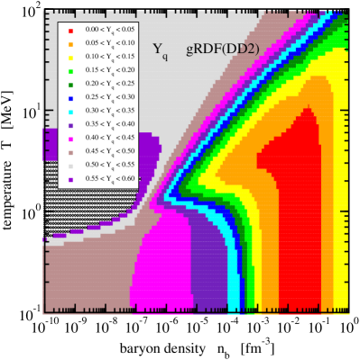
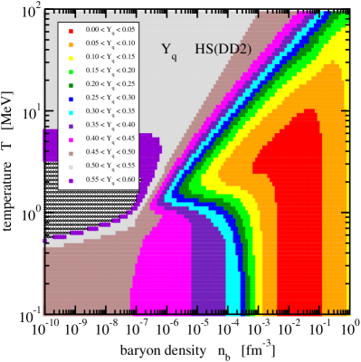
Figure 1: (Color online) Hadronic charge fraction $Y_{q}$ of neutron star matter for the gRDF model (a) and the HS model (b). The area of datapoints outside the EoS table ($Y_{q}$ larger than $0.6$) is indicated by crosses.

Properties of stellar matter are available for the gRDF and HS model for a large range of densities, temperatures and isospin asymmetries. In the present study they were extracted from EoS tables in the CompOSE format using the FORTRAN code compose.f90. In order to compare the two models, only a section through the full space of these variables is considered in the following. We restrict ourselves to the conditions of fully catalyzed neutron star matter, i.e., charge-neutral matter in $\beta$ equilibrium without neutrinos. Then, the hadronic charge fraction $Y_{q}$ is determined and the baryon density $n_{b}$ and the temperature $T$ remain as independent variables. In figure 1 the variation of $Y_{q}$ as a function of $n_{b}$ and $T$ is depicted for the gRDF and the HS model. Regions of different charge fraction values are color-coded in steps of 0.05. For baryon densities below approx. $10^{-7}$ fm^-3 and temperatures between $0.5$ MeV and $3$ MeV, $Y_{q}$ is above $0.6$ and thus outside the range of the EoS tables. In general, there is a rather good agreement of the predictions between the two models. For constant temperature, there is a decrease of the charge fraction with increasing baryon density as long as $n_{b}$ is lower than approx. $4\cdot 10^{-2}$ fm^-3. For $T>10$ MeV a further decrease of $Y_{q}$ with $n_{b}$ is observed, whereas the charge fraction increases at lower $T$ for the highest baryon densities. Above the nuclear saturation density, a somewhat larger difference in $Y_{q}$ between the models can be noticed because the gRDF model considers muons in contrast to the HS model. The lowest charge fractions with $Y_{q}<0.05$ are found for $T<10$ MeV in the baryon density range from roughly $5\cdot 10^{-3}$ fm^-3 to $10^{-1}$ fm^-3. At the lowest temperatures, the hadronic charge fraction evolves with $n_{b}$ as expected for cold neutron stars indicating the gradual neutronization of matter with increasing depth.

1 Chemical composition

The change of the hadronic charge fraction is accompanied with a change of the chemical composition in neutron star matter. The gRDF and HS models predict to some extent differences for both light and heavy nuclei. We first consider the isospin zero light nuclei. In figure 2 the mass fractions

$$X_{i}=A_{i}\frac{n_{i}}{n_{b}}$$ (109)

of deuterons and $\alpha$ particles, respectively, are depicted in the full range of baryon densities and temperatures. The contour lines of the color-coded regions denote a factor of ten change of the fractions. For temperatures below approx. $10$ MeV, an agreement of the two models is found to a large extent. In most cases, the $\alpha$-particle fraction exceeds that of the deuteron, except for densities above $10^{-2}$ fm^-3 and temperatures larger than approx. $4$ MeV. The maximum fractions of deuterons and, in particular $\alpha$ particles, are located in a rather narrow band of increasing density and temperature. At temperatures $T>20$ MeV, the largest differences between the models are observed. In the gRDF model, the net deuteron fraction decreases quickly with increasing temperature, for baryon densities $n_{b}<10^{-2}$ fm^-3, because the ground state contribution is compensated by the contribution of the corresponding scattering channel resulting in a disappearance of deuterons at higher temperatures. Contributions from two-nucleon scattering states are not considered in the HS model. Hence, the deuteron survives to much higher temperatures. For $\alpha$-particles, a compensating effect due to scattering states is neglected in both models because the ground state is much stronger bound as compared to the deuteron. In the HS model, the occurrence of clusters is suppressed at temperatures above $50$ MeV by introducing an artificial cutoff. This is most apparent for the $\alpha$-particle mass fractions in the bottom of figure 2.

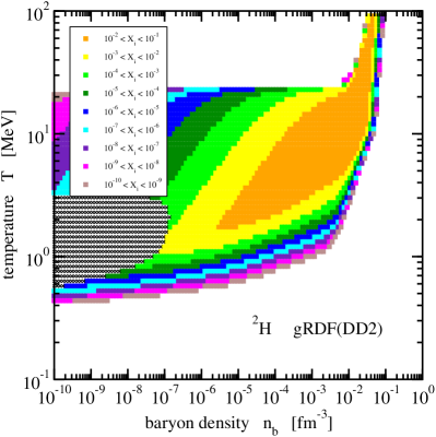
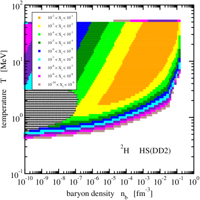
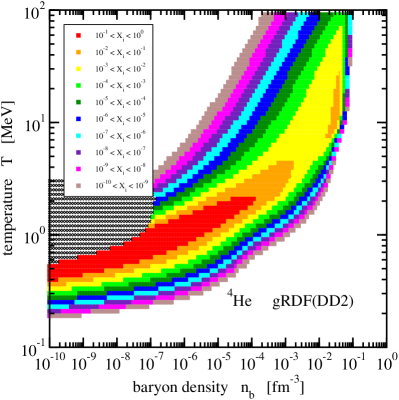
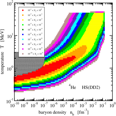
Figure 2: (Color online) Mass fraction $X_{d}$ of deuterons (²H) for the gRDF model (a) and the HS model (b) and mass fraction $X_{\alpha}$ of $\alpha$ particles (⁴He) for the gRDF model (c) and the HS model (d) in neutron star matter. The area of datapoints outside the EoS table is indicated by crosses.

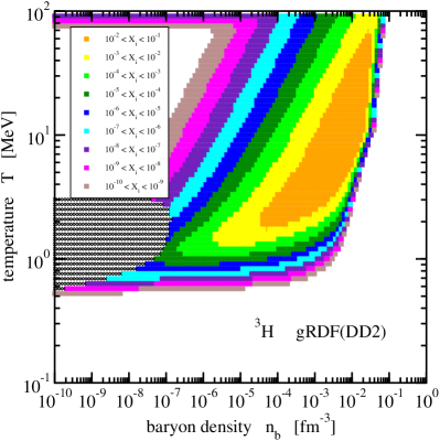
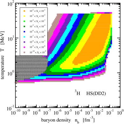
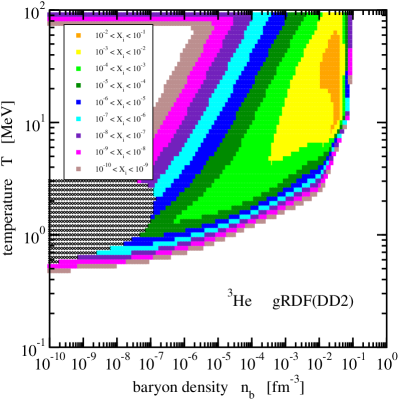
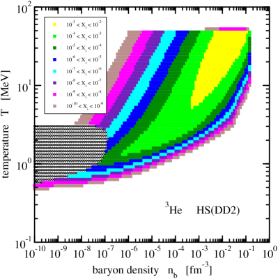
Figure 3: (Color online) Mass fraction $X_{t}$ of tritons (³H) for the gRDF model (a) and the HS model (b) and mass fraction $X_{h}$ of helions (³He) for the gRDF model (c) and the HS model (d) in neutron star matter. The area of datapoints outside the EoS table is indicated by crosses.

The observations for the deuteron and the $\alpha$ particle apply in a similar way to the ³H and ³He nuclei, with isospin $1/2$ and opposite neutron-to-proton composition. A comparison in figure 3 clearly shows that the more neutron-rich nucleus ³H is more likely to be found in neutron star matter with low hadronic charge fraction $Y_{q}$, c.f. figure 1, than the proton-rich nucleus ³He. In the gRDF model, both the triton and the helion are predicted to reappear at the highest temperatures for baryon densities below approx. $10^{-6}$ fm^-3. This can be explained by a simple thermodynamic consequence since for $T>70$ MeV binding energies have a rather minor effect on the distribution functions. A similar feature is expected for the HS model, if the cutoff for considering clusters was not introduced at $50$ MeV.

         

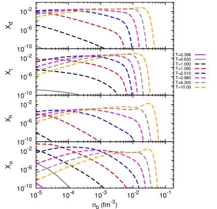
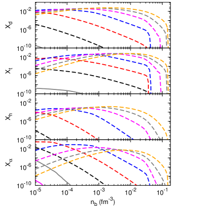
Figure 4: (Color online) Mass fractions of the light clusters, ²H (d), ³H (t), ³He (h) and ⁴He ($\alpha$) for the gRDF model (a) and for the HS model (b) for several isotherms.

  

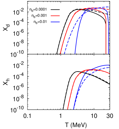
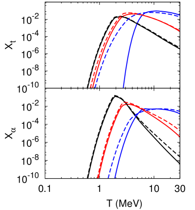
Figure 5: (Color online) Mass fractions of the light clusters, ²H (d), ³H (t), ³He (h) and ⁴He ($\alpha$), for the gRDF model (full lines) and the HS model (dashed lines) as a function of the temperature for different values of the baryon number density.

Larger differences in the predictions for light nuclei in the gRDF and HS model are visible for densities above $10^{-3}$ fm^-3. This becomes more apparent in figure 4, where the evolution of the mass fractions with density is depicted for several isotherms and a restricted density range, as compared to figures 2 and 3. At densities lower than approx. $10^{-3}$ fm^-3, the predictions of the two models are almost identical. Here, mass-shifts or excluded-volume effects hardly affect the mass fractions of light nuclei. But at higher densities, distinct differences appear. The HS model with excluded-volume mechanism predicts a more gradual dissolution of the light clusters with density than the gRDF model with mass shifts.

At temperatures below approx. $0.5-1.0$ MeV, light clusters are hardly found in neutron star matter. The variation of the mass fractions with temperature for three fixed values of the baryon number density $n_{b}$ are shown in figure 5. At low densities of $10^{-4}$ fm^-3 or $10^{-3}$ fm^-3, there are only minor differences between the gRDF and HS model in the mass fractions. Only at $10^{-2}$ fm^-3 the predictions of the models differ more strongly. There are larger discrepancies at lower temperatures because here differences in the cluster masses or excluded-volume effects are more relevant in the thermodynamic description. In case of the gRDF model, the net deuteron fraction rapidly decreases with temperature, when $T$ becomes larger than approx. $20$ MeV. This is caused by the continuum contribution in the np(${}^{3}S_{1}$) channel that compensates the deuteron ground state contribution.

  

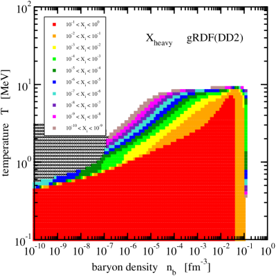
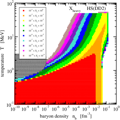
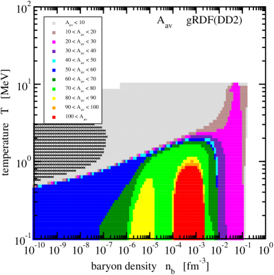
Figure 6: (Color online) Mass fraction $X_{\rm heavy}$ of heavy nuclei for the gRDF model (a) and the HS model (b) and average mass number $A_{\rm av}$ of heavy nuclei for the gRDF model (c) and the HS model (d) in neutron star matter. The area of datapoints outside the EoS table is indicated by crosses.

The chemical composition of neutron star matter at low temperatures is dominated by heavy nuclei with mass numbers $A>4$. This is evident from panels (a) and (b) of figure 6, that depict the total mass fraction of heavy nuclei

$$X_{\rm heavy}=\sum_{(A,Z),A>4}X_{(A,Z)}$$ (110)

with the mass fraction $X_{(A,Z)}=An_{(A,Z)}$ of individual nuclei as a function of baryon density and temperature. Below $T\approx 2$ MeV, the gRDF model and the HS model look very similar but the dissolution of heavy clusters occurs at lower densities in the HS model, in the range from $10^{-2}$ fm^-3 to $5\cdot 10^{-2}$ fm^-3, whereas heavy nuclei survive up to densities somewhat above $10^{-1}$ fm^-3. The disappearance of heavy nuclei with increasing temperature for constant baryon density shows some distinct differences, when the two models are compared. The $\gamma(T)$ factor in the degeneracy factor (71) of the gRDF model causes the heavy clusters to be removed from the system above approx. $10$ MeV. In the HS model, they appear at even higher temperatures, since the excluded-volume mechanism as a geometric concept is only depending on the density but not on the temperature. The reduction of $X_{\rm heavy}$ in the HS model with increasing temperature is only a consequence of statistics. In panel (b) of figure 6 we notice again the artificial cluster cutoff at $50$ MeV in this model.

  

  

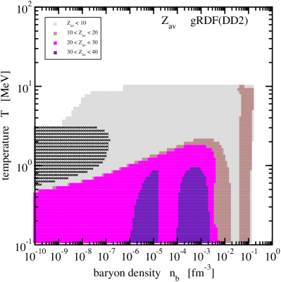
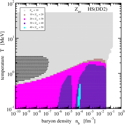
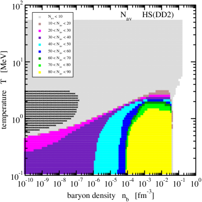
Figure 7: (Color online) Average charge number $Z_{\rm av}$ of heavy nuclei for the gRDF model (a) and the HS model (b) and average neutron number $N_{\rm av}$ of heavy nuclei for the gRDF model (c) and the HS model (d) in neutron star matter. The area of datapoints outside the EoS table is indicated by crosses.

In order to assess the importance of heavy nuclei in neutron star matter, not only the mass fraction $X_{\rm heavy}$, but also the size of the nuclei has to be examined. In panels (c) and (d) of figure 6 the variation of the average mass number

$$A_{\rm av}=\frac{1}{X_{\rm heavy}}\sum_{(A,Z),A>4}AX_{(A,Z)}$$ (111)

is illustrated, where the countour lines indicate a change by ten units. For baryon densities below $10^{-5}$ fm^-3, both models are very similar, and the expected increase of the average mass number with density is observed for the lowest temperatures. Above $10^{-5}$ fm^-3, however, the models exhibit significant differences. In the gRDF model, the highest average mass numbers are found for temperatures below $1$ MeV, in the density range from $10^{-4}$ fm^-3 to $2\cdot 10^{-3}$ fm^-3. At even higher densities, $A_{\rm av}$ continuously decreases to smaller values, before the heavy clusters dissolve, cf. panel (a) of figure 6. The situation is very different in the HS model. Here, the heaviest clusters survive almost until they disappear when the density increases. When the temperature increases above $3$ MeV, the average mass number of heavy nuclei quickly shrinks, and the chemical composition is governed by light clusters.

The change of the average mass numbers $A_{\rm av}$ is accompanied by a similar variation of the average charge number $Z_{\rm av}$ and the average neutron number $N_{\rm av}$ of heavy nuclei. These quantities are depicted in figure 7 for the gRDF model and the HS model in the same style as $A_{\rm av}$ in figure 6. The difference between the models are again clearly visible. Both $Z_{\rm av}$ and $N_{\rm av}$ decrease smoothly with increasing density above $2\cdot 10^{-3}$ fm^-3 for constant temperature below $2$ MeV in the gRDF model, and the maximum values are found in the density range from $10^{-4}$ fm^-3 to $2\cdot 10^{-3}$ fm^-3. In the HS model, large average charge and neutron number appear also at higher densities. Because the matter is very neutron rich, cf. figure 1, $N_{\rm av}$ reaches larger values than $Z_{\rm av}$. At the lowest temperatures, the sequence of charge and neutron numbers with increasing baryon density is similar to that expected in the crust of cold neutron stars.

         

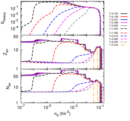
Figure 8: (Color online) Mass fraction $X_{\rm heavy}$, average charge number $Z_{\rm av}$ and average neutron number $N_{\rm av}$ of heavy nuclei as a function of the baryon number density $n_{b}$ for constant temperatures in the gRDF model (a) and in HS model (b).

The variation of $X_{\rm heavy}$, $Z_{\rm av}$ and $N_{\rm av}$ with increasing density for several isotherms in geometric progression is shown in figure 8, for a restricted range of densities. Heavy nuclei dominate the chemical composition at temperatures below approx. $0.6$ MeV and baryon densities below approx. $2\cdot 10^{-4}$ fm^-3, the neutron drip density in cold neutron star matter. In the HS model, heavy nuclei disappear abruptly at densities of about one fifth of the saturation density at low temperatures, but survive for temperatures above $1$ MeV also at higher densities. They dissolve at almost the same density of $n_{\rm sat}/3$, irrespective of the temperature in the gRDF model. Shell effects in the average charge and neutron numbers are clearly visible at low temperatures since the distribution of heavy nuclei is dominated by a few species. The jumps at the magic numbers are washed out with increasing temperature. A comparison of the gRDF results with those of the HS model shows that the size of the heavy clusters gradually reduces with increasing density in the former model but stays almost constant up to the dissolution density in the latter model.

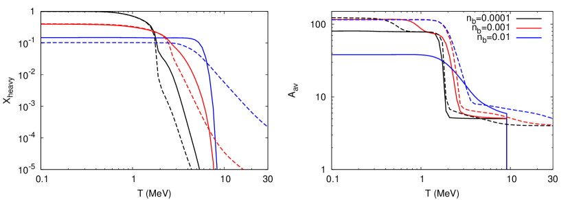
Figure 9: (Color online) Mass fraction $X_{\rm heavy}$ and average mass number $A_{\rm av}$ of heavy nuclei as a function of the temperature $T$ for constant baryon number densities $n_{b}$ in the gRDF model (full lines) and in the HS model (dashed lines).

The fraction of heavy nuclei and their average mass number as a function of the temperature for fixed baryon densities is depicted in figure 9. The dissolution of heavy nuclei with increasing temperature is evident with a steeper decrease in the gRDF model, where heavy nuclei are suppressed, if $T$ approaches $10$ MeV. At the highest density of $10^{-2}$ fm^-3, differences in $X_{\rm heavy}$ between the models, even at low temperatures, are observed. The evolution of the average mass fraction with temperature also exhibits clear differences, depending on the chosen value of $n_{b}$ in accordance with the lower panel of figure 6. The sudden change of $A_{\rm av}$ with the temperature at low $T$ is again related to shell effects that are taken care of in both models due to the use of realistic mass tables.

2 Thermodynamic properties

  

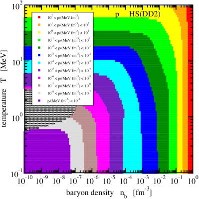
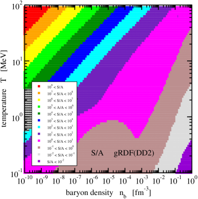
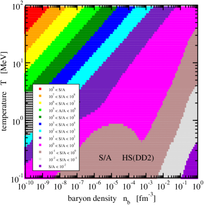
Figure 10: (Color online) Pressure $p$ for the gRDF model (a) and the HS model (b) and entropy per baryon $S/A$ for the gRDF model (c) and the HS model (d) in neutron star matter. The area of datapoints outside the EoS table is indicated by crosses.

Besides the chemical composition of neutron star matter, the predictions of the gRDF model and the HS model for thermodynamic quantities can be compared. As representative examples, the pressure $p$ and the entropy per baryon $S/A=s/n_{b}$ are depicted in figure 10 as a function of baryon density and temperature. The pressure and entropy per baryon along lines that separate differently colored regions differ by a factor of ten. There is a systematic increase of the pressure with $n_{b}$ and $T$ reaching the largest values at baryon densities approaching $1$ fm^-3. In contrast, the highest entropy per baryon is found at the highest temperatures close to $100$ MeV, at the lowest baryon densities. In general, $S/A$ decreases with decreasing temperature and increasing baryon density. There is an exception from this trend in the region close to the line of constant $S/A=1$, where the chemical composition of the matter rapidly changes. Overall there is a surprising agreement of the pressure and entropy per baryon between the two models, despite the very different approaches to model the dissolution of nuclei. A similar concordance of thermodynamic quantities, such as the free energy per baryon or chemical potentials is observed. Hence, we refrain from showing the corresponding figures.

4 Conclusions

In the present work, we presented and compared two different theoretical approaches to model the equation of state and in particular the formation and dissolution of nuclear clusters in stellar matter: a statistical model with excluded-volume effects (HS model) and a generalized relativistic density functional (gRDF model) with an in-medium change of the cluster masses. The theoretical formalism of the two approaches was presented in detail and the essential differences were delineated. Both models use a relativistic mean-field description for the nucleonic part with the same parametrisation of the density dependent meson-nucleon couplings, but they differ in the treatment of the cluster degrees of freedom. Data on the chemical composition and on thermodynamic properties are available in tabular form for both models in a wide range of baryon densities, temperatures and isospin asymmetries in the CompOSE format. The corresponding tables are taken from the CompOSE website.

We were interested mainly in the evolution of the light and heavy clusters with density and temperature. For that purpose, we studied neutron star matter, i.e. charge-neutral matter in $\beta$ equilibrium, and observed that the gRDF and the HS models predict some differences for the mass fractions and average sizes of the clusters. Both models behave similarly for low temperatures and low densities where mass shifts or excluded-volume effects are negligible. When the baryon density approaches the nuclear saturation density, the dissolution of clusters is more gradual in the gRDF model than in the HS model. Heavy clusters disappear rather abruptly with increasing density in the HS model, whereas in the gRDF model, their size gradually reduces until they melt.

Above temperatures of 50 MeV, light and heavy clusters are artificially suppressed in the HS model. In the gRDF model, heavy clusters are removed from the system when the temperature exceeds approximately $10$ MeV due to the specific temperature dependence of the degeneracy factors. In the HS model, they do appear at even higher temperatures, since the excluded-volume mechanism does not depend on the temperature, but only on the density.

Despite the differences in the cluster abundances and properties, both models show overall a very good agreement of the thermodynamic properties. Thus it can be expected that dynamical simulations of core-collapse supernovae or neutron star mergers are only marginally affected by the choice of the cluster description in the equation of state as long as the interaction model for the nucleonic part is identical. However, the chemical composition of stellar matter could affect processes such as the neutrino transport or nucleosynthesis in the above mentioned astrophysical scenarios. These consequences of the theoretical cluster description can be explored in future studies.

Acknowledgments

This work was supported by NewCompStar, COST Action MP1304, by the Helmholtz Association (HGF) through the Nuclear Astrophysics Virtual Institute (VH-VI-417), and by the DFG through grant No. SFB1245. H.P. is supported by FCT under Project No. SFRH/BPD/95566/2013. She is very thankful to S.T. and the Theory group at GSI for the kind hospitality during her stay there.

References

- 1. A. Mezzacappa, Ascertaining the Core Collapse Supernova Mechanism: The State of the Art and the Road Ahead, Ann. Rev. Nucl. Part. Sci. 55, 467–515 (2005). 10.1146/annurev.nucl.55.090704.151608.
- 2. H.-T. Janka, K. Langanke, A. Marek, G. Martinez-Pinedo, and B. Mueller, Theory of Core-Collapse Supernovae, Phys. Rept. 442, 38–74 (2007). 10.1016/j.physrep.2007.02.002.
- 3. H.-T. Janka, Explosion Mechanisms of Core-Collapse Supernovae, Ann. Rev. Nucl. Part. Sci. 62, 407–451 (2012). 10.1146/annurev-nucl-102711-094901.
- 4. A. Burrows, Colloquium: Perspectives on core-collapse supernova theory, Rev. Mod. Phys. 85, 245 (2013). 10.1103/RevModPhys.85.245.
- 5. N. K. Glendenning, Compact stars: Nuclear physics, particle physics, and general relativity. Springer, New York (1997).
- 6. F. Weber, Strange quark matter and compact stars, Prog.Part.Nucl.Phys. 54, 193–288 (2005). 10.1016/j.ppnp.2004.07.001.
- 7. P. Haensel, A. Y. Potekhin, and D. G. Yakovlev, Neutron stars 1: Equation of state and structure (2007).
- 8. A. Y. Potekhin, The physics of neutron stars, Phys. Usp. 53, 1235–1256 (2010). 10.3367/UFNe.0180.201012c.1279. [Usp. Fiz. Nauk180,1279(2010)].
- 9. J. M. Lattimer, The nuclear equation of state and neutron star masses, Ann.Rev.Nucl.Part.Sci. 62, 485–515 (2012). 10.1146/annurev-nucl-102711-095018.
- 10. K. Hebeler, J. M. Lattimer, C. J. Pethick, and A. Schwenk, Equation of state and neutron star properties constrained by nuclear physics and observation, Astrophys. J. 773, 11 (2013). 10.1088/0004-637X/773/1/11.
- 11. J. M. Lattimer and F. D. Swesty, A Generalized equation of state for hot, dense matter, Nucl. Phys. A535, 331–376 (1991). 10.1016/0375-9474(91)90452-C.
- 12. H. Shen, H. Toki, K. Oyamatsu, and K. Sumiyoshi, Relativistic equation of state of nuclear matter for supernova explosion, Prog. Theor. Phys. 100, 1013 (1998). 10.1143/PTP.100.1013.
- 13. H. Shen, H. Toki, K. Oyamatsu, and K. Sumiyoshi, Relativistic equation of state of nuclear matter for supernova and neutron star, Nucl. Phys. A637, 435–450 (1998). 10.1016/S0375-9474(98)00236-X.
- 14. T. Klähn et al., Constraints on the high-density nuclear equation of state from the phenomenology of compact stars and heavy-ion collisions, Phys. Rev. C74, 035802 (2006). 10.1103/PhysRevC.74.035802.
- 15. J. M. Lattimer and M. Prakash, Neutron Star Observations: Prognosis for Equation of State Constraints, Phys.Rept. 442, 109–165 (2007). 10.1016/j.physrep.2007.02.003.
- 16. M. Hempel and J. Schaffner-Bielich, Statistical Model for a Complete Supernova Equation of State, Nucl. Phys. A837, 210–254 (2010). 10.1016/j.nuclphysa.2010.02.010.
- 17. H. Shen, H. Toki, K. Oyamatsu, and K. Sumiyoshi, Relativistic Equation of State for Core-Collapse Supernova Simulations, Astrophys. J. Suppl. 197, 20 (2011). 10.1088/0067-0049/197/2/20.
- 18. G. Shen, C. J. Horowitz, and S. Teige, A New Equation of State for Astrophysical Simulations, Phys. Rev. C83, 035802 (2011). 10.1103/PhysRevC.83.035802.
- 19. G. Shen, C. J. Horowitz, and E. O’Connor, A Second Relativistic Mean Field and Virial Equation of State for Astrophysical Simulations, Phys. Rev. C83, 065808 (2011). 10.1103/PhysRevC.83.065808.
- 20. A. W. Steiner, M. Hempel, and T. Fischer, Core-collapse supernova equations of state based on neutron star observations, Astrophys. J. 774, 17 (2013). 10.1088/0004-637X/774/1/17.
- 21. M. Barranco and J. R. Buchler, Thermodynamic properties of hot nucleonic matter, Phys.Rev. C22, 1729–1737 (1980). 10.1103/PhysRevC.22.1729.
- 22. H. Muller and B. D. Serot, Phase transitions in warm, asymmetric nuclear matter, Phys.Rev. C52, 2072–2091 (1995). 10.1103/PhysRevC.52.2072.
- 23. K. Bugaev, M. I. Gorenstein, I. Mishustin, and W. Greiner, Exactly soluble model for nuclear liquid gas phase transition, Phys.Rev. C62, 044320 (2000). 10.1103/PhysRevC.62.044320.
- 24. F. Gulminelli, P. Chomaz, A. H. Raduta, and A. R. Raduta, The Influence of Coulomb on the liquid gas phase transition and nuclear multifragmentation, Phys. Rev. Lett. 91, 202701 (2003). 10.1103/PhysRevLett.91.202701.
- 25. C. Ducoin, P. Chomaz, and F. Gulminelli, Role of isospin in the nuclear liquid-gas phase transition, Nucl.Phys. A771, 68–92 (2006). 10.1016/j.nuclphysa.2006.03.005.
- 26. C. Ducoin, P. Chomaz, and F. Gulminelli, Isospin fractionation: Equilibrium versus spinodal decomposition, Nucl. Phys. A781, 407–423 (2007). 10.1016/j.nuclphysa.2006.11.047.
- 27. C. Ducoin, P. Chomaz, and F. Gulminelli, Isospin-dependent clusterization of Neutron-Star Matter, Nucl.Phys. A789, 403–425 (2007). 10.1016/j.nuclphysa.2007.03.006.
- 28. M. Hempel, T. Fischer, J. Schaffner-Bielich, and M. Liebendorfer, New Equations of State in Simulations of Core-Collapse Supernovae, Astrophys. J. 748, 70 (2012). 10.1088/0004-637X/748/1/70.
- 29. S. Furusawa, S. Yamada, K. Sumiyoshi, and H. Suzuki, A new baryonic equation of state at sub-nuclear densities for core-collapse simulations, Astrophys. J. 738, 178 (2011). 10.1088/0004-637X/738/2/178.
- 30. M. Hempel, V. Dexheimer, S. Schramm, and I. Iosilevskiy, Noncongruence of the nuclear liquid-gas and deconfinement phase transitions, Phys. Rev. C88(1), 014906 (2013). 10.1103/PhysRevC.88.014906.
- 31. S. Furusawa, K. Sumiyoshi, S. Yamada, and H. Suzuki, New equations of state based on the liquid drop model of heavy nuclei and quantum approach to light nuclei for core-collapse supernova simulations, Astrophys. J. 772, 95 (2013). 10.1088/0004-637X/772/2/95.
- 32. T. Fischer, M. Hempel, I. Sagert, Y. Suwa, and J. Schaffner-Bielich, Symmetry energy impact in simulations of core-collapse supernovae, Eur. Phys. J. A50, 46 (2014). 10.1140/epja/i2014-14046-5.
- 33. S. Typel, G. Röpke, T. Klähn, D. Blaschke, and H. H. Wolter, Composition and thermodynamics of nuclear matter with light clusters, Phys. Rev. C81, 015803 (2010). 10.1103/PhysRevC.81.015803.
- 34. C. J. Horowitz and A. Schwenk, Cluster formation and the virial equation of state of low-density nuclear matter, Nucl. Phys. A776, 55–79 (2006). 10.1016/j.nuclphysa.2006.05.009.
- 35. S. Heckel, P. P. Schneider, and A. Sedrakian, Light nuclei in supernova envelopes: a quasiparticle gas model, Phys. Rev. C80, 015805 (2009). 10.1103/PhysRevC.80.015805.
- 36. M. Ferreira and C. Providencia, Description of light clusters in relativistic nuclear models, Phys. Rev. C85, 055811 (2012). 10.1103/PhysRevC.85.055811.
- 37. S. S. Avancini, C. C. Barros, Jr., D. P. Menezes, and C. Providencia, particles and the pasta phase, Phys. Rev. C82, 025808 (2010). 10.1103/PhysRevC.82.025808.
- 38. S. S. Avancini, C. C. Barros, Jr, L. Brito, S. Chiacchiera, D. P. Menezes, and C. Providencia, Light clusters in nuclear matter and the ’pasta’ phase, Phys. Rev. C85, 035806 (2012). 10.1103/PhysRevC.85.035806.
- 39. D. G. Ravenhall, C. J. Pethick, and J. R. Wilson, Structure of matter below nuclear saturation density, Phys. Rev. Lett. 50, 2066–2069 (1983). 10.1103/PhysRevLett.50.2066.
- 40. R. D. Williams and S. E. Koonin, Sub-saturation phases of nuclear matter, Nucl. Phys. A. 435, 844 (1985).
- 41. C. J. Horowitz, M. A. Perez-Garcia, J. Carriere, D. K. Berry, and J. Piekarewicz, Nonuniform neutron-rich matter and coherent neutrino scattering, Phys. Rev. C70, 065806 (2004). 10.1103/PhysRevC.70.065806.
- 42. C. J. Horowitz, M. A. Perez-Garcia, D. K. Berry, and J. Piekarewicz, Dynamical response of the nuclear ’pasta’ in neutron star crusts, Phys. Rev. C72, 035801 (2005). 10.1103/PhysRevC.72.035801.
- 43. T. Maruyama, T. Tatsumi, D. N. Voskresensky, T. Tanigawa, and S. Chiba, Nuclear pasta structures and the charge screening effect, Phys. Rev. C72, 015802 (2005). 10.1103/PhysRevC.72.015802.
- 44. G. Watanabe, T. Maruyama, K. Sato, K. Yasuoka, and T. Ebisuzaki, Simulation of transitions between ’Pasta’ phases in dense matter, Phys. Rev. Lett. 94, 031101 (2005). 10.1103/PhysRevLett.94.031101.
- 45. H. Sonoda, G. Watanabe, K. Sato, K. Yasuoka, and T. Ebisuzaki, Phase diagram of nuclear ”pasta” and its uncertainties in supernova cores, Phys. Rev. C77, 035806 (2008). 10.1103/PhysRevC.77.035806, 10.1103/PhysRevC.81.049902. [Erratum: Phys. Rev.C81,049902(2010)].
- 46. H. Pais and J. R. Stone, Exploring the Nuclear Pasta Phase in Core-Collapse Supernova Matter, Phys. Rev. Lett. 109, 151101 (2012). 10.1103/PhysRevLett.109.151101.
- 47. F. Grill, H. Pais, C. Providencia, I. Vidaña, and S. S. Avancini, Equation of state and thickness of the inner crust of neutron stars, Phys. Rev. C90(4), 045803 (2014). 10.1103/PhysRevC.90.045803.
- 48. C. J. Horowitz, M. A. Perez-Garcia, and J. Piekarewicz, Neutrino - pasta scattering: The Opacity of nonuniform neutron - rich matter, Phys. Rev. C69, 045804 (2004). 10.1103/PhysRevC.69.045804.
- 49. H. Sonoda, G. Watanabe, K. Sato, T. Takiwaki, K. Yasuoka, and T. Ebisuzaki, The impact of nuclear pasta on neutrino transport in collapsing cores, Phys. Rev. C75, 042801 (2007). 10.1103/PhysRevC.75.042801.
- 50. M. D. Alloy and D. P. Menezes, Nuclear ’pasta phase’ and its consequences on neutrino opacities, Phys. Rev. C83, 035803 (2011). 10.1103/PhysRevC.83.035803.
- 51. S. Furusawa, H. Nagakura, K. Sumiyoshi, and S. Yamada, The influence of inelastic neutrino reactions with light nuclei on the standing accretion shock instability in core-collapse supernovae, Astrophys. J. 774, 78 (2013). 10.1088/0004-637X/774/1/78.
- 52. P. Haensel, Composition of dense matter and neutrino cooling of neutron stars, Acta Phys.Polon. B25, 373–399 (1994).
- 53. D. Page and S. Reddy, Forecasting neutron star temperatures: predictability and variability, Phys. Rev. Lett. 111(24), 241102 (2013). 10.1103/PhysRevLett.111.241102.
- 54. B. Haskell and A. Melatos, Models of Pulsar Glitches, Int. J. Mod. Phys. D24(03), 1530008 (2015). 10.1142/S0218271815300086.
- 55. E. Salpeter, Energy and Pressure of a Zero-Temperature Plasma, Astrophys.J. 134, 669–682 (1961). 10.1086/147194.
- 56. G. Baym, C. Pethick, and P. Sutherland, The Ground state of matter at high densities: Equation of state and stellar models, Astrophys.J. 170, 299–317 (1971). 10.1086/151216.
- 57. P. Haensel and B. Pichon, Experimental nuclear masses and the ground state of cold dense matter, Astron.Astrophys. 283, 313 (1994).
- 58. F. Douchin and P. Haensel, A unified equation of state of dense matter and neutron star structure, Astron. Astrophys. 380, 151 (2001). 10.1051/0004-6361:20011402.
- 59. S. B. Ruester, M. Hempel, and J. Schaffner-Bielich, The outer crust of non-accreting cold neutron stars, Phys. Rev. C73, 035804 (2006). 10.1103/PhysRevC.73.035804.
- 60. J. M. Pearson, S. Goriely, and N. Chamel, Properties of the outer crust of neutron stars from Hartree-Fock-Bogoliubov mass models, Phys. Rev. C83, 065810 (2011). 10.1103/PhysRevC.83.065810.
- 61. R. N. Wolf et al., Plumbing Neutron Stars to New Depths with the Binding Energy of the Exotic Nuclide 82Zn, Phys. Rev. Lett. 110(4), 041101 (2013). 10.1103/PhysRevLett.110.041101.
- 62. A. S. Botvina and I. N. Mishustin, Formation of hot heavy nuclei in supernova explosions, Phys. Lett. B584, 233–240 (2004). 10.1016/j.physletb.2004.01.064.
- 63. A. S. Botvina and I. N. Mishustin, Statistical approach for supernova matter, Nucl. Phys. A843, 98–132 (2010). 10.1016/j.nuclphysa.2010.05.052.
- 64. S. I. Blinnikov, I. V. Panov, M. A. Rudzsky, and K. Sumiyoshi, The equation of state and composition of hot, dense matter in core-collapse supernovae, Astron. Astrophys. 535, A37 (2011). 10.1051/0004-6361/201117225.
- 65. A. R. Raduta and F. Gulminelli, Thermodynamics of clusterized matter, Phys. Rev. C80, 024606 (2009). 10.1103/PhysRevC.80.024606.
- 66. A. R. Raduta and F. Gulminelli, Statistical description of complex nuclear phases in supernovae and proto-neutron stars, Phys. Rev. C82, 065801 (2010). 10.1103/PhysRevC.82.065801.
- 67. F. Gulminelli and A. R. Raduta, Ensemble in-equivalence in supernova matter within a simple model, Phys. Rev. C85, 025803 (2012). 10.1103/PhysRevC.85.025803.
- 68. N. Buyukcizmeci et al., A comparative study of statistical models for nuclear equation of state of stellar matter, Nucl. Phys. A907, 13–54 (2013). 10.1016/j.nuclphysa.2013.03.010.
- 69. N. Buyukcizmeci, A. S. Botvina, and I. N. Mishustin, Tabulated equation of state for supernova matter including full nuclear ensemble, Astrophys. J. 789, 33 (2014). 10.1088/0004-637X/789/1/33.
- 70. A. R. Raduta, F. Aymard, and F. Gulminelli, Clusterized nuclear matter in the (proto-)neutron star crust and the symmetry energy, Eur. Phys. J. A50, 24 (2014). 10.1140/epja/i2014-14024-y.
- 71. V. V. Sagun, A. I. Ivanytskyi, K. A. Bugaev, and I. N. Mishustin, The statistical multifragmentation model for liquid-gas phase transition with a compressible nuclear liquid, Nucl. Phys. A924, 24–46 (2014). 10.1016/j.nuclphysa.2013.12.012.
- 72. M. Hempel, J. Schaffner-Bielich, S. Typel, and G. Röpke, Light Clusters in Nuclear Matter: Excluded Volume versus Quantum Many-Body Approaches, Phys. Rev. C84, 055804 (2011). 10.1103/PhysRevC.84.055804.
- 73. S. Typel, Variations on the excluded-volume mechanism, Eur. Phys. J. A52(1), 16 (2016). 10.1140/epja/i2016-16016-3.
- 74. T. Klähn, M. Oertel, and S. Typel. CompOSE: Compstar Online Supernova Equations of State. http://compose.obspm.fr (2013–2014).
- 75. K. Sumiyoshi and G. Roepke, Appearance of light clusters in post-bounce evolution of core-collapse supernovae, Phys. Rev. C77, 055804 (2008). 10.1103/PhysRevC.77.055804.
- 76. G. Röpke, Parametrization of light nuclei quasiparticle energy shifts and composition of warm and dense nuclear matter, Nucl. Phys. A867, 66–80 (2011). 10.1016/j.nuclphysa.2011.07.010.
- 77. G. Röpke, N. U. Bastian, D. Blaschke, T. Klähn, S. Typel, and H. H. Wolter, Cluster virial expansion for nuclear matter within a quasiparticle statistical approach, Nucl. Phys. A897, 70–92 (2013). 10.1016/j.nuclphysa.2012.10.005.
- 78. G. Röpke, Quantum statistical calculation of cluster abundances in hot dense matter, J. Phys. Conf. Ser. 436, 012070 (2014). 10.1088/1742-6596/436/1/012070. [436,012070(2013)].
- 79. G. Röpke, Nuclear matter equation of state including two-, three-, and four-nucleon correlations, Phys. Rev. C92(5), 054001 (2015). 10.1103/PhysRevC.92.054001.
- 80. M. D. Voskresenskaya and S. Typel, Constraining mean-field models of the nuclear matter equation of state at low densities, Nucl. Phys. A887, 42–76 (2012). 10.1016/j.nuclphysa.2012.05.006.
- 81. S. Typel. Equation of State in a Generalized Relativistic Density Functional Approach. In Compact Stars in the QCD Phase Diagram IV Prerow, Germany, September 26-30, 2014 (2015). URL https://inspirehep.net/record/1358250/files/arXiv:1504.01571.pdf.
- 82. S. Typel and H. H. Wolter, Relativistic mean field calculations with density dependent meson nucleon coupling, Nucl. Phys. A656, 331–364 (1999). 10.1016/S0375-9474(99)00310-3.
- 83. M. Wang, G. Audi, A. Wapstra, F. Kondev, M. Mac-Cormick, X. Xu, and B. Pfeiffer, The AME2012 atomic mass evaluation (II). Tables, graphs and references, Chinese Physics C. 36, 1603 (Dec., 2012). 10.1088/1674-1137/36/12/003.
- 84. J. Duflo and A. P. Zuker, Microscopic mass formulae, Phys. Rev. C52, R23 (1995). 10.1103/PhysRevC.52.R23.
- 85. M. K. Grossjean and H. Feldmeier, Level density of a Fermi gas with pairing interactions, Nucl. Phys. 444, 113–132 (1985).
- 86. G. Audi, A. Wapstra, and C. Thibault, The AME2003 atomic mass evaluation: (II). Tables, graphs and references, Nucl. Phys. 729, 337 (2003). 10.1016/j.nuclphysa.2003.11.003.
- 87. P. Moller, J. R. Nix, W. D. Myers, and W. J. Swiatecki, Nuclear ground state masses and deformations, Atom. Data Nucl. Data Tabl. 59, 185–381 (1995). 10.1006/adnd.1995.1002.