Linear Superiorization for Infeasible Linear Programming

Linear Superiorization for Infeasible Linear Programming

Abstract

Linear superiorization (abbreviated: LinSup) considers linear programming (LP) problems wherein the constraints as well as the objective function are linear. It allows to steer the iterates of a feasibility-seeking iterative process toward feasible points that have lower (not necessarily minimal) values of the objective function than points that would have been reached by the same feasiblity-seeking iterative process without superiorization. Using a feasibility-seeking iterative process that converges even if the linear feasible set is empty, LinSup generates an iterative sequence that converges to a point that minimizes a proximity function which measures the linear constraints violation. In addition, due to LinSup’s repeated objective function reduction steps such a point will most probably have a reduced objective function value. We present an exploratory experimental result that illustrates the behavior of LinSup on an infeasible LP problem.

1 Introduction: The General Concept of Superiorization

Given an algorithmic operator $\mathcal{A}:X\rightarrow X$ on a Hilbert space $X$, consider the iterative process

$$x^{0}\in X,\;x^{k+1}=\mathcal{A}\left(x^{k}\right),\;\mathrm{for}\,\mathrm{all}\;k\geqslant 0,$$ (1)

and let $SOL\left(P\right)$ denote the solution set of some problem $P$ of any kind. The iterative process is said to solve $P$ if, under some reasonable conditions, any sequence $\left\{x^{k}\right\}_{k=0}^{\infty}$ generated by the process converges to some $x^{*}\in SOL\left(P\right)$. An iterative process (1) that solves $P$ is called perturbation resilient if the process

$$y^{0}\in X,\;y^{k+1}=\mathcal{A}\left(y^{k}+v^{k}\right),\;\mathrm{for}\,\mathrm{all}\;k\geqslant 0,$$ (2)

also solves $P$, under some reasonable conditions on the sequence of perturbation vectors $\left\{v^{k}\right\}_{k=0}^{\infty}\subseteq X$. The iterative processes of (1) and (2) are called “the basic algorithm” and “the superiorized version of the basic algorithm”, respectively.

Superiorization aims at identifying perturbation resilient iterative processes that will allow to use the perturbations in order to steer the iterates of the superiorized algorithm so that, while retaining the original property of converging to a point in $SOL\left(P\right)$, they will also do something additional useful for the original problem $P$, such as converging to a point with reduced values of some given objective function. These concepts are rigorously defined in several recent works in the field, we refer the reader to the recent reviews [13],[5] and references therein. More material about the current state of superiorization can be found also in [6], [14] and [19].

A special case of prime importance and significance of the above is when $P$ is a convex feasibility problem (CFP) of the form: Find a vector $x^{*}\in\cap_{i=1}^{I}C_{i}$ where $C_{i}\subseteq R^{J}$, the $J$-dimensional Euclidean space, are closed convex subsets, and the perturbations in the superiorized version of the basic algorithm are designed to reduce the value of a given objective function $\phi$.

In this case the basic algorithm (1) can be any of the wide variety of feasibility-seeking algorithms, see, e.g., [2], [8] and [7], and the perturbations employ nonascent directions of $\phi$. Much work has been done on this as can be seen in the Internet bibliography at [4].

The usefulness of this approach is twofold: First, feasibility-seeking is, on a logical basis, a less-demanding task than seeking a constrained minimization point in a feasible set. Therefore, letting efficient feasibility-seeking algorithms “lead” the algorithmic effort and modifying them with inexpensive add-ons works well in practice.

Second, in some real-world applications the choice of an objective function is exogenous to the modeling and data acquisition which give rise to the constraints. Thus, sometimes the limited confidence in the usefulness of a chosen objective function leads to the recognition that, from the application-at-hand point of view, there is no need, neither a justification, to search for an exact constrained minimum. For obtaining “good results”, evaluated by how well they serve the task of the application at hand, it is often enough to find a feasible point that has reduced (not necessarily minimal) objective function value.

2 Linear Superiorization

2.1 The problem and the algorithm

Let the feasible set $M$ be

$$M:=\{x\in R^{J}\mid Ax\leq b,\text{ }x\geq 0\}$$ (3)

where the $I\times J$ real matrix $A=(a_{j}^{i})_{i=1,j=1}^{I,J}$ and the vector $b=(b_{i})_{i=1}^{I}\in R^{I}$ are given.

For a basic algorithm we pick a feasibility-seeking projection method. Here projection methods refer to iterative algorithms that use projections onto sets while relying on the general principle that when a family of, usually closed and convex, sets is present, then projections onto the individual sets are easier to perform than projections onto other sets (intersections, image sets under some transformation, etc.) that are derived from the individual sets.

Projection methods may have different algorithmic structures, such as block-iterative projections (BIP) or string-averaging projections (SAP) (see, e.g., the review paper [9] and references therein) of which some are particularly suitable for parallel computing, and they demonstrate nice convergence properties and/or good initial behavior patterns.

This class of algorithms has witnessed great progress in recent years and its member algorithms have been applied with success to many scientific, technological and mathematical problems. See, e.g., the 1996 review [2], the recent annotated bibliography of books and reviews [7] and its references, the excellent book [3], or [8].

An important comment is in place here. A CFP can be translated into an unconstrained minimization of some proximity function that measures the feasibility violation of points. For example, using a weighted sum of squares of the Euclidean distances to the sets of the CFP as a proximity function and applying steepest descent to it results in a simultaneous projections method for the CFP of the Cimmino type. However, there is no proximity function that would yield the sequential projections method of the Kaczmarz type, for CFPs, see [1].

Therefore, the study of feasibility-seeking algorithms for the CFP has developed independently of minimization methods and it still vigorously does, see the references mentioned above. Over the years researchers have tried to harness projection methods for the convex feasibility problem to LP in more than one way, see, e.g., Chinneck’s book [11].

The mini-review of relations between linear programming and feasibility-seeking algorithms in [17, Section 1] sheds more light on this. Our work in [6] and here leads us to study whether LinSup can be useful for either feasible or infeasible LP problems.

The objective function for linear superiorization will be

$$\phi(x):=\left\langle c,x\right\rangle$$ (4)

where $\left\langle c,x\right\rangle$ is the inner product of $x$ and a given $c\in R^{J}.$

In the footsteps of the general principles of the superiorization methodology, as presented for general objective functions $\phi$ in previous publications, we use the following linear superiorization (LinSup) algorithm. The algorithm and its implementation details follow closely those of [6] wherein only feasible constraints were discussed.

The input to the algorithm consists of the problem data $A,$ $b,$ and $c$ of (3) and (4), respectively, a user-chosen initialization point $\bar{y}$ and a user-chosen parameter (called here kernel) $0<\alpha<1$ with which the algorithm generates the step-sizes $\beta_{k,n}$ by the powers of the kernel $\eta_{\ell}=\alpha^{\ell},$ as well as an integer $N$ that determines the quantity of objective function reduction perturbation steps done per each feasibility-seeking iterative sweep through all linear constraints. The perturbation direction $-\frac{{\displaystyle c}}{{\displaystyle\left\|c\right\|_{2}}}$ used in step 10 of Algorithm 1 is a nonascend direction of the linear objective function, as required by the general principles of the superiorization methodology, see, e.g., [14, Subsection II.D].

Algorithm 1. The Linear Superiorization (LinSup) Algorithm

1. set $k=0$

2. set $y^{k}=\bar{y}$

3. set $\ell_{-1}=0$

4. while stopping rule not met do

5.       set $n=0$

6. set $\ell=rand(k,\ell_{k-1})$

7.       set $y^{k,n}=y^{k}$

8.       while $n$$<$$N$ do

9.             set $\beta_{k,n}=\eta_{\ell}$

10.             set $z=y^{k,n}-\beta_{k,n}\frac{{\displaystyle c}}{{\displaystyle\left\|c\right\|_{2}}}$

11.             set $n\leftarrow n+1$

12.             set $y^{k,n}$$=$$z$

13. set $\ell\leftarrow\ell+1$

14. end while

15. set $\ell_{k}=\ell$

16. set $y^{k+1}$$=$$\mathcal{A}\left(y^{k,N}\right)$

17. set $k\leftarrow k+1$

18. end while

All quantities in this algorithm are detailed and explained below, except for the choice of the basic algorithm for the feasibility-seeking operator represented by $\mathcal{A}$ in step 16 of Algorithm 2.1 which appear in the next subsection.

Step-sizes of the perturbations. The step sizes $\beta_{k,n}$ in Algorithm 1 must be such that $0<\beta_{k,n}\leq 1$ in a way that guarantees that they form a summable sequence $\sum_{k=0}^{\infty}\sum_{n=0}^{N-1}\beta_{k,n}<\infty,$ see, e.g., [10]. To this end Algorithm 1 assumes that we have available a summable sequence $\{\eta_{\ell}\}_{\ell=0}^{\infty}$ of positive real numbers generated by $\eta_{\ell}=\alpha^{\ell}$ , where $0<\alpha<1$. Simultaneously with generating the iterative sequence $\{y^{k}\}_{k=0}^{\infty},$ a subsequence of $\{\eta_{\ell}\}_{\ell=0}^{\infty}$ is used to generate the step sizes $\beta_{k,n}$ in step 9 of Algorithm 1. The number $\alpha$ is called the kernel of the sequence $\{\eta_{\ell}\}_{\ell=0}^{\infty}.$

Controlling the decrease of the step-sizes of objective function reduction. If during the application of Algorithm 1 the step sizes $\beta_{k,n}$ decrease too fast then too little leverage is allocated to the objective function reduction activity that is interlaced into the feasibility-seeking activity of the basic algorithm. This delicate balance can be controlled by the choice of the index $\ell$ updates and separately by the value of $\alpha$ whose powers $\alpha^{\ell}$ determine the step sizes $\beta_{k,n}$ in step 9. In our work we adopt a strategy for updating the index $\ell$ that was proposed and implemented for total variation (TV) image reconstruction from projections by Prommegger and by Langthaler in [18, page 38 and Table 7.1 on page 49] and in [15], respectively. This strategy advocates to set $\ell$ at the beginning of every new iteration sweep (steps 5 and 6) to a random number between the current iteration index $k$ and the value of $\ell$ from the last iteration sweep, i.e., $\ell_{k}=rand(k,\ell_{k-1}).$

The proximity function. To measure the feasibility-violation (or level of disagreement) of a point with respect to the target set $M$ we used the following proximity function

$$\Pr(x):=\frac{1}{2I}{\displaystyle\sum_{i=1}^{I}}\frac{\left(\left(\left\langle a^{i},x\right\rangle-b_{i}\right)_{+}\right)^{2}}{{\displaystyle\sum\limits_{j=1}^{J}}\left(a_{j}^{i}\right)^{2}}+\frac{1}{2J}{\displaystyle\sum\limits_{j=1}^{J}}\left(\left(-x_{j}\right)_{+}\right)^{2}$$ (5)

where the plus notation means, for any real number $d,$ that $d_{+}:=\max(d,0).$

The number $N$ of perturbation steps. This number $N$ of perturbation steps that are performed prior to each application of the feasibility-seeking operator $\mathcal{A}$ (in step 16) affects the performance of the LinSup algorithm. It influences the balance between the amounts of computations allocated to feasibility-seeking and those allocated to objective function reduction steps. A too large $N$ will make Algorithm 1 spend too much resources on the perturbations that yield objective function reduction.

Handling the nonnegativity constraints. The nonnegativity constraints in (3) are handled by projections onto the nonnegative orthant, i.e., by taking the iteration vector in hand after each iteration of Cimmino’s feasibility-seeking algorithm applied to all $I$ row-inequalities of (3) and setting its negative components to zero while keeping the others unchanged.

2.2 Cimmino’s feasibility-seeking algorithm as the basic algorithm

We use the simultaneous projections method of Cimmino for linear inequalities, see, e.g. [12], as the basic algorithm for the feasibility-seeking operator represented by$\mathcal{A}$ in step 16 of Algorithm 1. Denoting the half-spaces represented by individual rows of (3) by $H_{i},$

$$H_{i}:=\{x\in R^{J}\mid\left\langle a^{i},x\right\rangle\leq b_{i}\},$$ (6)

where $a^{i}\in R^{J}$ is the $i$-th row of $A$ and $b_{i}\in R$ is the $i$-th component of $b$ in (3), he orthogonal projection of an arbitrary point $z\in R^{J}$ onto $H_{i},$ has the closed-form

$$P_{H_{i}}(z)=\left\{\begin{array}[]{ll}z-{\displaystyle\frac{\left\langle a^{i},z\right\rangle-b_{i}}{\|a^{i}\|^{2}}a^{i},}&\text{if }\left\langle a^{i},z\right\rangle>b_{i},\\ z,&\text{if }\left\langle a^{i},z\right\rangle\leq b_{i}.\end{array}\right.$$ (7)

Algorithm 2. The Simultaneous Feasibility-Seeking Projection Method of Cimmino

Initialization: $x^{0}\in R^{J}$ is arbitrary.

Iterative step: Given the current iteration vector $x^{k}$ the next iterate is calculated by

$$x^{k+1}=x^{k}+\lambda_{k}\left(\sum_{i=1}^{I}w_{i}\left(P_{H_{i}}(x^{k})-x^{k}\right)\right)$$ (8)

with weights $w_{i}\geq 0$ for all $i\in I,$ and $\sum_{i=1}^{I}w_{i}=1.$

Relaxation parameters: The parameters $\lambda_{k}$ are such that $\epsilon_{1}\leq\lambda_{k}\leq 2-\epsilon_{2},$ for all $k\;\geq\;0,$ with some, arbitrarily small, fixed, $\epsilon_{1},\epsilon_{2}>0.$

This Cimmino simultaneous feasibility-seeking projection algorithm is known to generate convergent iterative sequences even if the intersection $\cap_{i=1}^{I}H_{i}$ is empty, as the following, slightly paraphrased, theorem tells.

Theorem 2.1

[12, Theorem 3] For any starting point $x^{0}\in R^{J}$, any sequence $\{x^{k}\}_{k=0}^{\infty},$ generated by the simultaneous feasibility-seeking projection method of Cimmino (Algorithm 2) converges. If the underlying system of linear inequalities is consistent, the limit point is a feasible point for it. Otherwise, the limit point minimizes $f(x):=\sum_{i=1}^{I}w_{i}\parallel P(x)-x\parallel^{2}$, i.e., it is a weighted (with the weights $w_{i}$) least squares solution of the system.

3 An Empirical Result

Employing MATLAB 2014b [16], we created five test problems each with 2500 linear inequalities in $R^{J},\>J=2000$. The entries in 1250 rows of the matrix $A$ in (3) were uniformly distributed random numbers from the interval $(-1,1).$ The remaining 1250 rows were defined as the negatives of the first 1250 rows, i.e., $a_{j}^{1250+t}=-a_{j}^{t}$ for all $t=1,2,\ldots,1250$ and all $j=1,2,\ldots,2000.$ This guarantees that the two sets of rows represent parallel half-spaces with opposing normals. For the right-hand side vectors, the components of $b$ associated with the first set of 1250 rows in (3) were uniformly distributed random numbers from the interval $(0,100).$ The remaining 1250 components of each $b$ were chosen as follows: $b_{1250+t}=-b_{t}-rand(100,200)$ for all $t=1,2,\ldots,1250$. This guarantees that the distance between opposing parallel half-spaces is large making them inconsistent, i.e., having no point in common, and that the whole system is infeasible.

For the linear objective function, the components of $c$ were uniformly distributed random numbers from the interval $(-2,1).$ All runs of Algorithm 1 and Algorithm 2 were initialized at $\bar{y}=10\cdot\mathbf{1}$ and $x^{0}=10\cdot\mathbf{1}$, respectively, where $\mathbf{1}$ is the vector of all 1’s.

We ran Algorithm 1 on each problem until it ceased to make progress, by using the stopping rule

$$\frac{{\displaystyle\left\|y^{k}-y^{k-1}\right\|}}{\left\|y^{k}\right\|}\leq 10^{-4}.$$ (9)

The same stopping rule was used for runs of Algorithm 2. The relaxation parameters in Cimmino’s feasibility-seeking basic algorithm in step 16 of Algorithm 1 were fixed with $\lambda_{k}=1.99$ for all $k\geqslant 0.$ Based on our work in [6] we used $N=20$ and $\alpha=0.99$ in steps 8 and 9 of Algorithm 1, respectively, where $\eta_{\ell}=\alpha^{\ell}.$

The three figures, presented below, show results for the five different (but similarly generated) families of inconsistent linear inequalities along with nonnegativity constraints. Figures 1 and 2, in particular, show that the perturbation steps 5-15 of the LinSup Algorithm 1 initially work and reduce the objective function value powerfully during the first ca. 500 iterative sweeps (an iterative sweep consists of one pass through steps 5-17 in Algorithm 1 or one pass through all linear inequalities and the nonnegativity constraints in Algorithm 2). As iterative sweeps proceed the perturbations in Algorithm 1 loose steam because of the decreasing values of the $\beta_{k,n}$s and later the algorithm proceeds toward feasibility at the expense of some increase of objective function values. However, even at those later sweeps the objective function values of LinSup remain well below those of the unsuperiorized application of the Cimmino feasibility-seeking algorithm (Algorithm 2).

The slow increase of objective function values observed for the unsuperiorized application of the Cimmino feasibility-seeking algorithm seems intriguing because the feasibility-seeking algorithm is completely unaware of the given objective function $\phi(x):=\left\langle c,x\right\rangle.$ But this is understood from the fact that the unsuperiorized algorithm has an orbit of iterates in $R^{J}$ which, by proceeding in space toward proximity minimizers, crosses the linear objective function’s level sets in a direction that either increases or decreases objective function values. It would keep them constant only if the orbit was confined to a single level set of $\phi$ which is not a probable thing to happen. To clarify this we recorded in Figure 3 the values of $\left\langle c,x\right\rangle$ and $\left\langle-c,x\right\rangle$ at the iterates $x^{k}$ produced by the Cimmino feasibility-seeking algorithm (Algorithm 2).

Figure 1: Linear objective function values plotted against iteration sweeps. LinSup has reduced objective function values although the effect of objective function reducing perturbations diminishes as iterations proceed.

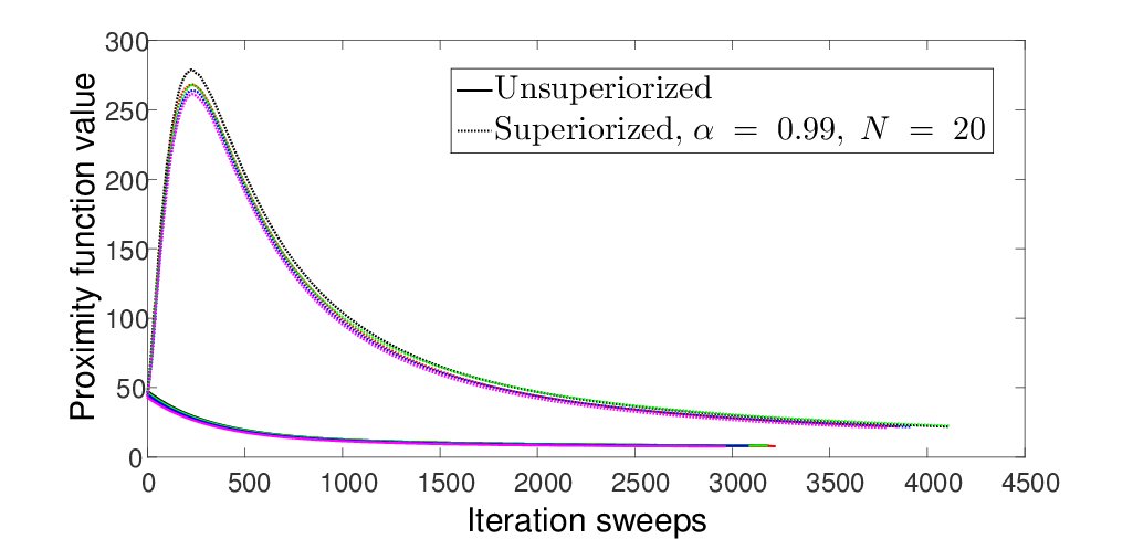
Figure 2: Proximity function values plotted against iteration sweeps. The unsuperiorized feasibility-seeking only algorithm does a better job than LinSup here which is understandable. LinSup’s strive for feasibility comes at the expense of some increase in objective function values, as seen in Figure 1.

Figure 3: The fact that objective function values increase to some extent by the unsuperiorized feasibility-seeking only algorithm observed in Figure 1 is due to the relative situation of the linear objective function’s level sets with respect to where in space is the set of proximity minimizers of the infeasible target set.

Concluding Comments

We proposed a new approach to handle infeasible linear programs (LPs) via the linear superiorization (LinSup) method. To this end we applied the feasibility-seeking projection method of Cimmino to the original linear infeasible constraints (without using additional variables). This Cimmino method is guaranteed to converge to one of the points that minimize a proximity function that measures the violation of all constraints. We used the given linear objective function to superiorize Cimmino’s method to steer its iterates to proximity minimizers with reduced objective function values. Further computational research is needed to evaluate and compare the results of this new approach to existing solution approaches to infeasible LPs.

Acknowledgments. We thank Gabor Herman, Ming Jiang and Evgeni Nurminski for reading a previous version of the paper and sending us comments that helped improve it. This work was supported by Research Grant No. 2013003 of the United States-Israel Binational Science Foundation (BSF).

References

- [1] J-B. Baillon, P. L. Combettes, and R. Cominetti. There is no variational characterization of the cycles in the method of periodic projections. Journal of Functional Analysis, 262:400–408, 2012.
- [2] H.H. Bauschke and J.M. Borwein. On projection algorithms for solving convex feasibility problems. SIAM Review, 38:367–426, 1996.
- [3] A. Cegielski. Iterative methods for fixed point problems in Hilbert spaces, volume 2057. Springer-Verlag, Berlin, Heidelberg, Germany, 2012.
- [4] Y. Censor. Superiorization and Perturbation Resilience of Algorithms: A Bibliography compiled and continuously updated by Yair Censor. Available at: http://math.haifa.ac.il/yair/bib-superiorization-censor.htm.
- [5] Y. Censor. Weak and strong superiorization: Between feasibility-seeking and minimization. Analele Stiintifice ale Universitatii Ovidius Constanta-Seria Matematica, 23:41–54, 2015.
- [6] Y. Censor. Can linear superiorization be useful for linear optimization problems? Technical report, under review, 2016.
- [7] Y. Censor and A. Cegielski. Projection methods: an annotated bibliography of books and reviews. Optimization, 64:2343–2358, 2015.
- [8] Y. Censor, W. Chen, P. L. Combettes, R. Davidi, and G. T. Herman. On the effectiveness of projection methods for convex feasibility problems with linear inequality constraints. Computational Optimization and Applications, 51:1065–1088, 2012.
- [9] Y. Censor and A. Segal. Iterative projection methods in biomedical inverse problems. In Y. Censor, M. Jiang, and A. K Louis, editors, Mathematical Methods in Biomedical Imaging and Intensity-Modulated Radiation Therapy (IMRT), pages 65–96. Edizioni della Normale, Pisa, Italy, 2008.
- [10] Y. Censor and A. J. Zaslavski. Strict Fejér monotonicity by superiorization of feasibility-seeking projection methods. Journal of Optimization Theory and Applications, 165:172–187, 2015.
- [11] J. W. Chinneck. Feasibility and Infeasibility in Optimization: Algorithms and Computational Methods. Springer Science+Business Media, LLC, New York, NY, USA, 2008.
- [12] A. R. De Pierro and A. N. Iusem. A simultaneous projections method for linear inequalities. Linear Algebra and Its applications, 64:243–253, 1985.
- [13] G. T. Herman. Superiorization for image analysis. In Combinatorial Image Analysis: 16th International Workshop, IWCIA 2014, Brno, Czech Republic, pages 1–7. Lecture Notes in Computer Science, Volume 8466. Springer, 2014.
- [14] G. T. Herman, E. Garduño, R. Davidi, and Y. Censor. Superiorization: An optimization heuristic for medical physics. Medical Physics, 39:5532–5546, 2012.
- [15] O. Langthaler. Incorporation of the superiorization methodology into biomedical imaging software. Marshall Plan Scholarship Report, Salzburg University of Applied Sciences, Salzburg, Austria, and The Graduate Center of the City University of New York, NY, USA, 76 pages, 2014.
- [16] MATLAB. A high-level language and interactive environment system by The Mathworks Inc., Natick, MA, USA. http://www.mathworks.com/products/matlab/.
- [17] E. A. Nurminski. Single-projection procedure for linear optimization. Journal of Global Optimization, pages 1–16, 2015.
- [18] B. Prommegger. Verification and evaluation of superiorized algorithms used in biomedical imaging: Comparison of iterative algorithms with and without superiorization for image reconstruction from projections. Marshall Plan Scholarship Report, Salzburg University of Applied Sciences, Salzburg, Austria, and The Graduate Center of the City University of New York, NY, USA, 84 pages, 2014.
- [19] D. Reem and A. De Pierro. A new convergence analysis and perturbation resilience of some accelerated proximal forward-backward algorithms with errors. arXiv preprint arXiv:1508.05631, 2015.
- [20] H. A. Simon. Rational choice and the structure of the environment. Psychological Review, 63:129–138, 1956.