Proposal for Gravitational-Wave Detection Beyond the Standard Quantum Limit via EPR Entanglement

Abstract

The Standard Quantum Limit in continuous monitoring of a system is given by the trade-off of shot noise and back-action noise. In gravitational-wave detectors, such as Advanced LIGO, both contributions can simultaneously be squeezed in a broad frequency band by injecting a spectrum of squeezed vacuum states with a frequency-dependent squeeze angle. This approach requires setting up an additional long base-line, low-loss filter cavity in a vacuum system at the detector’s site. Here, we show that the need for such a filter cavity can be eliminated, by exploiting EPR-entangled signal and idler beams. By harnessing their mutual quantum correlations and the difference in the way each beam propagates in the interferometer, we can engineer the input signal beam to have the appropriate frequency dependent conditional squeezing once the out-going idler beam is detected. Our proposal is appropriate for all future gravitational-wave detectors for achieving sensitivities beyond the Standard Quantum Limit.

Background and Summary.– Detection of gravitational waves from merging binary black holes (BBH) by the Laser Interferometer Gravitational-wave Observatory (LIGO) opened the era of gravitational wave astronomy GW150914 . The future growth of the field relies on the improvement of detector sensitivity, and the vision for ground-based gravitational-wave detection is to improve, eventually by a factor $\sim$30 in amplitude in the next 30 years Punturo2010 ; Danilishin2012 ; Miao2014 ; Dwyer2015 ; GWsensitivity . This will eventually allow us to observe all BBH mergers that take place in the universe, thereby inform on the formation mechanism of BBH, the evolution of the universe Dwyer2015 ; Sathyaprakash2012 , and the way gravitational waves propagate through the universe Tso2016 ; Kostelecky2016 . Higher signal-to-noise ratio observations of BBH will allow demonstrations and tests of effects of general relativity in the strong gravity and nonlinear regimes Lasky2016 ; Berti2013 . Besides BBH, gravitational waves from neutron stars are being highly anticipated, as well as an active program of joint EM-GW observations Chu2016 ; Metzger2012 . Finally, improved sensitivity may lead to detections of more exotic sources cosmicstring2014 , as well as surprises.

A key toward better detector sensitivity is to suppress quantum noise, which arises from the quantum nature of light and the mirrors, and is driven by vacuum fluctuations of the optical field entering from the dark port of the interferometer Drever1976 ; Braginsky1977 ; Weiss1979 ; Caves1981 . There are two types of quantum noise: shot noise, the finite displacement resolution due to the finite number of photons, and the radiation-pressure noise, which arises from the photons randomly impinging on the mirrors. In the broadband configuration of Advanced LIGO, we measure the phase quadrature of the carrier field at the dark port, the quadrature that contains GW signal. In this case, shot noise is driven by phase fluctuations of the incoming optical field, while radiation-pressure noise is driven by amplitude fluctuations. The trade off between these two types of noise, as dictated by the Heisenberg Uncertainty Principle, gives rise to a sensitivity limitation called the Standard Quantum Limit (SQL) Kimble2001 ; Buonanno2001 ; Buonanno2003 .

One way to improve LIGO’s sensitivity with minimal modification to its optical configuration is to inject squeezed vacuum into the dark port Caves1981 ; Unruh1982 ; Schnabel2010 ; LIGOwhitepaper . More than 10 dB of squeezing down to audio side-band frequency (10 Hz to 10 kHz) has been demonstrated in the lab Vahlbruch2008 ; Mehmet2011 ; Chua2011 ; Stefszky2012 ; McKenzie2004 ; Vahlbruch2016 , while moderate noise reductions have been demonstrated in the large-scale interferometers GEO 600 squeezingLIGO2011 and LIGO squeezingLIGO2013 . However, squeezed vacuum generated by a nonlinear crystal via Optical Parametric Amplification (OPA) is frequency-independent for audio sidebands: within the GW band, we can only “squeeze” a fixed quadrature — fluctuations in the orthogonal quadrature are amplified by the same factor, as required by the Heisenberg Uncertainty Principle. This does not allow broadband improvement of sensitivity beyond the SQL Jaekel1990 ; Kimble2001 such as the example shown in Fig. 1; instead, a frequency-dependent quadrature must be squeezed for each sideband frequency. Starting off from frequency-independent squeezing, we must rotate the squeezed quadrature in a frequency-dependent way Kimble2001 ; Chelkowski2005 ; for the broadband configuration of Advanced LIGO, this rotation angle needs to gradually transition by $\pi/2$ at a frequency scale of 50 Hz Evans2013 . Kimble et al. Kimble2001 proposed to achieve such rotation by filtering the field with two Fabry-Perot cavities; Khalili further showed that it is often sufficient to use one cavity with bandwidth and detuning (from the carrier frequency) roughly at the transition frequency Khalili2007 ; Khalili2010 . However, the narrowness of the bandwidth requires the filter cavity to be long in order to limit impact from optical losses; the current plan for Advanced LIGO is to construct a $\sim 16$ m filter cavity Isogai2013 ; Evans2013 ; Kwee2014 , and $\sim 300$m long cavities have been studied for KAGRA Caposcasa2016 and for the Einstein Telecscope ET2011 . Alternative theoretical proposals for creating narrowband filter cavities were also discussed, they are strongly limited by thermal noise and/or optical losses Mikhailov2006 ; Ma2014 ; Qin2014 .

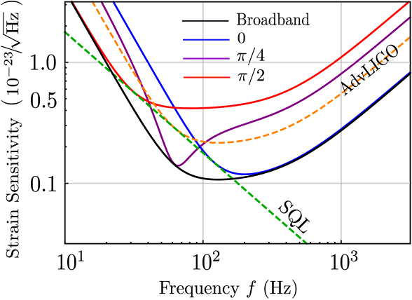
Figure 1: Sensitivity of a AdvLIGO type gravitational wave detector driven by squeezed vacuum (6 dB squeeze degree is chosen for comparing the $5\%$ input/output loss case in Fig. 4) with a fixed squeezing angle. The red, purple and blue curves describe the cases when squeezed light is injected with squeezing angle $0$(corresponding to an amplitude squeezed vacuum), $\pi/4$ and $\pi/2$, respectively. The black curve is the case when there is a frequency dependent squeezed vacuum injection.

In this paper, we propose a novel strategy to achieve broadband squeezing of the total quantum noise via the preparation of EPR entanglement and the dual use of the interferometer as both the GW detector and the filter, eliminating the need for external filter cavities.

As shown in Fig. 2, our strategy is divided into 4 steps. (i) We detune the pumping frequency of the OPA away from $2\omega_{0}$ (where $\omega_{0}$ is the carrier frequency of the interferometer) to $\omega_{p}=2\omega_{0}+\Delta$, with $\Delta$ an rf frequency of a few MHz, creating two EPR-entangled beams: the signal beam around the carrier frequency $\omega_{0}$, and the idler beam around $\omega_{0}+\Delta$. (ii) The idler beam, being far detuned from the carrier, sees the interferometer as a simple detuned cavity, and experiences frequency-dependent quadrature rotation, see Fig. 3, which can be optimised by adjusting $\Delta$ with respect to the lengths of interferometer cavities. (iii)

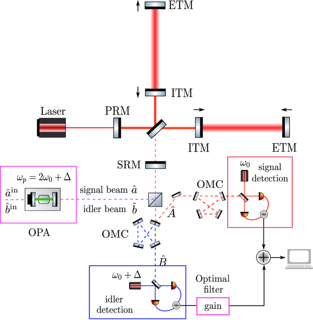
Figure 2: Optical configuration for noise suppression via EPR entanglement. The OPA is detuned by $\Delta$, generating signal beam $a$ and idler beam $b$ and injecting them into the interferometer. Upon returning from the interferometer, signal beam $A$ and idler beam $B$ are separated and filtered by the output mode cleaners (denoted as OMC in the figure), and each detected via homodyne detection. Measurement data are combined using an optimal filter for obtaining the squeezing of the quantum noise on the signal channel. The abbreviations PRM, ITM, ETM and SRM stand for power recycling mirror, input test mass mirror, end test mass mirror and signal recycling mirror, respectively.

When traveling out of the interferometer, the collinear signal and idler beams are separated and filtered by the output mode cleaners and measured by beating with local oscillators at frequencies $\omega_{0}$ and $\omega_{0}+\Delta$, respectively. (iv) The homodyne measurement of a fixed quadrature of the out-going idler beam conditionally squeezes the input signal beam in a frequency dependent way, thereby achieving the broadband reduction of quantum noise. Practically, benefit of the conditional squeezing of the signal beam is obtained as we apply a Wiener filter to the photocurrent of the idler and subtract it from the photocurrent of the signal beam. Without optical losses, using parameters in Table 2 (with a 15 dB squeezed vacuum in particular), we obtain the solid black curve in Fig. 4, with $\sim$11-12 dB improvement over the entire frequency band. We shall next discuss more details of the configuration, as well as the impact of optical losses; further details are provided as Supplementary Materials.

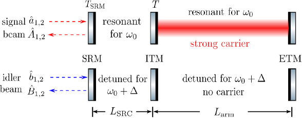
Figure 3: The differential mode of the interferometer as seen by the signal (upper panel) and idler (lower panel) beams.

$\lambda$	Carrier laser wavelength	1064 nm
$T_{\rm SRM}$	SRM power transmissivity	0.35
$T$	ITM power transmissivity	0.014
$L_{\rm arm}$	Arm cavity length	$\sim 4$ km
$L_{\rm SRC}$	Signal recycling cavity length	$\sim 50$ m
$\gamma$	Detection bandwidth	389 Hz
$m$	Mirror mass (ITM and ETM)	40 kg
$I_{c}$	Intra cavity power	650 kW
$\Delta$	Idler-signal detuning	$-15.3$ MHz
$r$	Squeeze factor of the OPA	1.23 (15  dB)

Table 1: Sample Parameters for Advanced LIGO. (See supplementary material for details.)

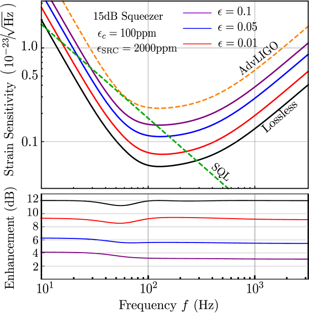
Figure 4: Upper panel: Noise spectrum of Advanced LIGO configurations with conditional frequency-dependent squeezing by using a 15 dB squeezed vacuum at MHz frequencies(see Table 2), assuming no loss (black), and assuming arm-cavity loss $\epsilon_{c}=100\,$ppm and signal recycling cavity loss $\epsilon_{\rm SRC}=2000\,$ppm, plus an identical input and output loss $\epsilon$ of 1% (red), 5% (blue) and 10% (purple). Lower panel: The sensitivity improvement factor measured in terms of dB.

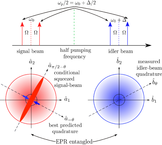
Figure 5: Spectral decomposition of EPR-entangled beams (upper panel) and the quantum statics of the signal and idler beams (lower panel).

EPR entanglement by detuning the OPA.–

For an OPA pumped at $\omega_{p}$, it is often convenient to study quadrature fields around $\omega_{p}/2$, which are linear combinations of upper and lower sideband fields at $\omega_{p}/2\pm\Omega$, with $\zeta$ quadrature defined by:

$$\hat{c}_{\zeta}(\Omega)=\left(e^{-i\zeta}\hat{c}_{\omega_{p}/2+\Omega}+e^{+i\zeta}\hat{c}_{\omega_{p}/2-\Omega}^{\dagger}\right)/\sqrt{2}$$ (1)

Here $\hat{c}_{\omega}$ and $\hat{c}^{\dagger}_{\omega}$ are the annihilation and creation operators for the optical field at $\omega$; we will use $\hat{c}_{1,2}$ to stand for $\hat{c}_{0,\pi/2}$, and $\hat{c}_{\zeta}=\hat{c}_{1}\cos\zeta+\hat{c}_{2}\sin\zeta$. For a squeeze factor $r$ and squeeze angle $\theta$, the orthogonal quadratures $\hat{c}_{\theta}$ and $\hat{c}_{\theta+\pi/2}$ have uncorrelated fluctuations, with spectra given by

$$S_{\hat{c}_{\theta}\hat{c}_{\theta}}=e^{-2r}\,,\;S_{\hat{c}_{\theta+{\pi/2}}\hat{c}_{\theta+{\pi/2}}}=e^{+2r}\,.$$ (2)

Compared with vacuum, fluctuations in $\hat{c}_{\theta}$ are suppressed by $e^{2r}$, and those in $\hat{c}_{\theta+\pi/2}$ are amplified by $e^{2r}$. This is due to the entanglement between the upper and lower sidebands, $\omega_{p}/2\pm\Omega$, generated by the optical nonlinearity. However, any pair of sideband fields with frequencies $\omega_{1}$ and $\omega_{2}$ within the squeeze bandwidth (usually $>$MHz) from $\omega_{p}/2$, and satisfying $\omega_{1}+\omega_{2}=\omega_{p}$, are entangled; in particular, for the proposed OPA (Fig. 2) with pumping frequency $\omega_{p}=2\omega_{0}+\Delta$, we have entanglement between $\omega_{0}+\Omega$ and $\omega_{0}+\Delta-\Omega$, as well as $\omega_{0}-\Omega$ and $\omega_{0}+\Delta+\Omega$, as shown in the upper panel of Fig. 5. As it turns out, this entanglement is equivalent to an EPR-type entanglement Zhang2003 ; Marino2007 ; Hage2010 between quadratures around $\omega_{0}$ [consisting of $\omega_{0}\pm\Omega$ sidebands, denoted by $\hat{a}_{\zeta}(\Omega)$] and those around $\omega_{0}+\Delta$ [consisting $\omega_{0}+\Delta\pm\Omega$ sidebands, denoted by $\hat{b}_{\zeta}(\Omega)$]. In terms of the four fields, $(\hat{a}_{1}\pm\hat{b}_{1})/\sqrt{2}$ and $(\hat{a}_{2}\pm\hat{b}_{2})/\sqrt{2}$, they are mutually uncorrelated, and have spectra

$$S_{(\hat{a}_{1}\pm\hat{b}_{1})/{\sqrt{2}}}=e^{\pm 2r}\,,\quad S_{({\hat{a}_{2}\pm\hat{b}_{2}})/{\sqrt{2}}}=e^{\mp 2r}\,.$$ (3)

In other words, for $r\stackrel{{\scriptstyle>}}{{{}_{\sim}}}1$, fluctuations in $\hat{b}_{1}-\hat{a}_{1}$ and $\hat{b}_{2}+\hat{a}_{2}$ are both much below vacuum level, as in the original EPR situation. In this way (lower panel of Fig. 5), if we detect $\hat{b}_{\theta}=\hat{b}_{1}\cos\theta+\hat{b}_{2}\sin\theta$, we can predict $\hat{a}_{-\theta}=\hat{a}_{1}\cos\theta-\hat{a}_{2}\sin\theta$ with a very good accuracy, while not providing any information for $\hat{a}_{\pi/2-\theta}$. More precisely, given measurement data of the idler quadrature $\hat{b}_{\theta}$, the signal beam will be conditionally squeezed, with conditional spectra

$$S^{|\hat{b}_{\theta}}_{\hat{a}_{-\theta}\hat{a}_{-\theta}}={1}/{\cosh(2r)}\,,\;S^{|\hat{b}_{\theta}}_{\hat{a}_{\frac{\pi}{2}-\theta}\hat{a}_{\frac{\pi}{2}-\theta}}=\cosh(2r)\,,$$ (4)

where the squeeze angle is $-\theta$, and the squeeze factor is $(\log\,\cosh(2r))/2$. For significant squeezing, $e^{2r}\gg 1$, this corresponds to 3 dB less squeezing than before detuning the pump field.

Improvement of Detector Sensitivity.– As shown in Fig.1, after signal beam $\hat{a}_{1,2}$ and idler beam $\hat{b}_{1,2}$ are fed into the interferometer, we detect phase quadratures of the out-going signal and the idler beams, $A_{2}$ and $B_{2}$, after they are separated and filtered by the output mode cleaners (Fig. 2). For the signal beam (upper panel of Fig. 3), we have Kimble2001 :

$$\hat{A}_{2}=e^{2i\beta}(\hat{a}_{2}-\mathcal{K}\hat{a}_{1})+\sqrt{2\mathcal{K}}e^{i\beta}h/h_{\rm SQL}\,,$$ (5)

which consists of shot noise, radiation-pressure noise, and signal, with $\beta=\arctan(\Omega/\gamma)$, where $\gamma$ is the bandwidth of the interferometer seen by the signal beam,

$$h^{2}_{\rm SQL}={8\hbar}/{(m\Omega^{2}L^{2})},\quad\mathcal{K}=2\Theta^{3}\gamma/[\Omega^{2}(\Omega^{2}+\gamma^{2})],$$ (6)

and $\Theta=[8\omega_{0}I_{c}/(mLc)]^{1/3}$.

Here we need to squeeze the $a_{[-\arctan(1/\mathcal{K})]}$ quadrature of the input signal beam, which requires detecting $b_{\arctan(1/\mathcal{K})}$. If we detect $B_{2}$, we will need the interferometer (lower panel of Fig. 3) to apply a rotation of $\Phi_{\rm rot}=\arctan\mathcal{K}$ to the idler beam so that $\hat{B}_{2}=\hat{b}_{\arctan(1/\mathcal{K})}$. This can be realized approximately by adjusting the detuning $\Delta$ and the length of signal-recycling cavity and arm cavity (see Supplementary Material for details), if $\Theta\ll\gamma$. To achieve the sensitivity provided by conditional squeezing, we need to compute the best estimate of $\hat{A}_{2}$ from $\hat{B}_{2}$, and subtract it from $\hat{A}_{2}$. If a rotation by $\Phi_{\rm rot}$ is realized exactly, we will have a noise spectrum of

$$S_{h}\approx\frac{h_{\rm SQL}^{2}}{2\cosh{2r}}\left(\mathcal{K}+\frac{1}{\mathcal{K}}\right),$$ (7)

where conditional squeezing provides a $\cosh\,2r$ suppression. In reality, we get less suppression since the interferometer, acting as a single cavity, does not exactly realize $\Phi_{\rm rot}$ for the idler beam. In Fig. 4, the black curve shows the actual noise spectrum for parameters in Table 2.

Discussions.– In Fig. 4, we plot noise spectra of interferometers with optical losses. In particular, we include losses in the arm cavities, at the input port, and during readout. As it turns out, the current 100 ppm arm cavity loss and 2000 ppm has only a small effect on the noise (for details, see Supplementary Material). When the input loss and the readout loss are both around $10\%$, the sensitivity improvement is only roughly $3$ dB, which corresponds to an amplitude improvement $\sim 1.4$. However, for a lower loss of 5%, which is promising in the near future Evans2013 ; Barsotti2016 ; Barsotti2014 , we can gain 6 dB or a factor of $\sim 2$ improvement in amplitude. This corresponds to an increase of sensitive sky volume by a factor of 8. Compared to the traditional scheme with a filter cavity Evans2013 , our input and detection losses are doubled, because signal and idler beams experience the same amount of loss during propagation. Although we do suffer less from loss in the filter cavity compare to the design based on an auxiliary filter cavity (since arm cavities have less loss), this higher level of input and detection losses is the price we have to pay in this scheme for eliminating the additional filter cavity.

Acknowledgements.– Research of YM, BHP, YC is supported by NSF grant PHY-1404569 and PHY-1506453, as well as the Institute for Quantum Information and Matter, a Physics Frontier Center. H.M. is supported by the Marie-Curie Fellowship and UK STFC Ernest Rutherford Fellowship. CZ would like to thank the support of Australian Research Council Discovery Project DP120104676 and DP120100898. RS is supported by DFG grant SCHN757/6 and by ERC grant 339897 (‘Mass Q’)

I Supplementary Material

II Derivation of the sensitivity formula

First, for each audio-sideband frequency $\Omega$, the field input-output relations of the squeezer (the pumped OPA) can be written as:

$$\begin{split}&\hat{a}(\omega_{0}+\Omega)=\mu\hat{a}_{\rm in}(\omega_{0}+\Omega)+\nu\hat{b}^{\dagger}_{\rm in}(\omega_{0}+\Delta-\Omega),\quad\hat{b}(\omega_{0}+\Delta+\Omega)=\mu\hat{b}_{\rm in}(\omega_{0}+\Delta+\Omega)+\nu\hat{a}^{\dagger}_{\rm in}(\omega_{0}-\Omega);\\ &\hat{a}^{\dagger}(\omega_{0}-\Omega)=\mu^{*}\hat{a}^{\dagger}_{\rm in}(\omega_{0}-\Omega)+\nu^{*}\hat{b}_{\rm in}(\omega_{0}+\Delta+\Omega),\quad\hat{b}^{\dagger}(\omega_{0}+\Delta-\Omega)=\mu^{*}\hat{b}^{\dagger}_{\rm in}(\omega_{0}+\Delta-\Omega)+\nu^{*}\hat{a}_{\rm in}(\omega_{0}+\Omega),\end{split}$$ (8)

where $\hat{a}$ and $\hat{b}$ describe the generated signal and idler fields near $\omega_{0}$ and $\omega_{0}\pm\Delta$, respectively. The fields $\hat{a}_{\rm in},\hat{b}_{\rm in}$ represent the vacuum fields entering into the squeezer. The phenomenological coefficient $\mu$ and $\nu$ are determined by the $\chi^{(2)}-$nonlinearity coefficient of the crystal and the pumping field strength [1]. Field commutation relation requires them to satisfy the relation $|\mu^{2}|-|\nu|^{2}=1$. Since the phase of $\mu$ and $\nu$ can be absorbed into the definition of creation and annihilation operators, we can parametrise them as $\mu=\cosh{r}$ and $\nu=\sinh{r}$, where $r$ is usually denoted to be the squeezing degree of the OPA. In the so-called two-photon formalism where we define:

$$\begin{split}&\hat{a}_{1}(\Omega)=\frac{\hat{a}(\omega_{0}+\Omega)+\hat{a}^{\dagger}(\omega_{0}-\Omega)}{\sqrt{2}},\quad\hat{b}_{1}(\Omega)=\frac{\hat{b}(\omega_{0}+\Delta+\Omega)+\hat{b}^{\dagger}(\omega_{0}+\Delta-\Omega)}{\sqrt{2}};\\ &\hat{a}_{2}(\Omega)=\frac{\hat{a}(\omega_{0}+\Omega)-\hat{a}^{\dagger}(\omega_{0}-\Omega)}{\sqrt{2}i},\quad\hat{b}_{2}(\Omega)=\frac{\hat{b}(\omega_{0}+\Delta+\Omega)-\hat{b}^{\dagger}(\omega_{0}+\Delta-\Omega)}{\sqrt{2}i},\\ \end{split}$$ (9)

the relations in Eq. (8) then can be represented in another form (in the following, $\hat{a}_{1,2}(\Omega)$ and $\hat{b}_{1,2}(\Omega)$ will be simply written as $\hat{a}_{1,2}$ and $\hat{b}_{1,2}$):

$$\hat{a}_{1}+\hat{b}_{1}=e^{r}(\hat{a}_{\rm in1}+\hat{b}_{\rm in1}),\quad\hat{a}_{1}-\hat{b}_{1}=e^{-r}(\hat{a}_{\rm in1}-\hat{b}_{\rm in1});$$ (10)

$$\hat{a}_{2}+\hat{b}_{2}=e^{-r}(\hat{a}_{\rm in2}+\hat{b}_{\rm in2}),\quad\hat{a}_{2}-\hat{b}_{2}=e^{r}(\hat{a}_{\rm in2}-\hat{b}_{\rm in2}),$$ (11)

(the $\hat{a}_{\rm in1,2},\hat{b}_{\rm in1,2}$ are defined in the same way as Eq. (9)). EPR-type commutation relation $[\hat{a}_{1}-\hat{b}_{1},\hat{a}_{2}+\hat{b}_{2}]=0$ allows the existence of the state in which the fluctuations of quadrature combinations $(\hat{a}_{1}-\hat{b}_{1})/\sqrt{2}$ and $(\hat{a}_{2}+\hat{b}_{2})/\sqrt{2}$ are much below the vacuum level. Therefore $\hat{b}_{1}$ is correlated with $\hat{a}_{1}$ while $\hat{b}_{2}$ is correlated with $-\hat{a}_{2}$. Therefore $\hat{a}_{-\theta}=\hat{a}_{1}\cos\theta-\hat{a}_{2}\sin\theta$ correlates with $\hat{b}_{\theta}=\hat{b}_{1}\cos\theta+\hat{b}_{2}\sin\theta$. When we do conditioning by combining the measurement results of signal and idler fields, we assume the measurement result of the idler field quadrature $\hat{b}_{\theta}$ is filtered with a filtering gain factor $g$ and then combined with the signal field quadrature $\hat{a}_{-\theta}$, leads to:

$$\hat{a}^{g}_{-\theta}=\hat{a}_{-\theta}-g\hat{b}_{\theta}=(\hat{a}_{1}-g\hat{b}_{1})\cos\theta-(\hat{a}_{2}+g\hat{b}_{2})\sin\theta.$$ (12)

It is easy to show that the spectrum of $\hat{a}^{g}_{-\theta}$ is:

$$S_{\hat{a}^{g}_{-\theta}\hat{a}^{g}_{-\theta}}=(\mu-g\nu)^{2}+(\nu-g\mu)^{2}.$$ (13)

For realising an optimal filtering (which is the so-called “Wiener filtering") so that $S_{\hat{a}^{g}_{-\theta}\hat{a}^{g}_{-\theta}}$ takes its minimum value, we can solve $\delta S_{\hat{a}^{g}_{-\theta}\hat{a}^{g}_{-\theta}}/\delta g=0$, which leads to the Wiener filter gain factor $g_{\rm opt}$ and conditional squeezing spectrum:

$$g_{\rm opt}=\frac{2\mu\nu}{\mu^{2}+\nu^{2}}=\tanh{2r},\quad S^{\rm cond}_{\hat{a}_{-\theta}\hat{a}_{-\theta}}=\frac{1}{\mu^{2}+\nu^{2}}=\frac{1}{\cosh{2r}}.$$ (14)

In laser interferometer gravitational wave detectors, we have the input-output relation for quantum noise field in the signal channel as [2]:

$$\begin{split}&\hat{A}_{2}=e^{2i\beta}(\hat{a}_{2}-\mathcal{K}\hat{a}_{1})=e^{2i\beta}(\sqrt{1+\mathcal{K}^{2}})(\hat{a}_{1}\cos\xi-\hat{a}_{2}\sin\xi),\\ \end{split}$$ (15)

where $\hat{A}_{2}$ is the phase quadrature of the signal fields propagate out of the interferometer and $\xi=-\arctan{1/\mathcal{K}}$. If we want the phase quadrature of the idler fields out of the interferometer $\hat{B}_{2}$ to maximally correlate with $\hat{A}_{2}$ in Eq. (15), then $\hat{B}_{2}=\hat{b}_{\rm\arctan{1/\mathcal{K}}}$ (besides an unimportant phase factor $\alpha$ accumulated by sidebands of the idler field during its propagation ). Therefore, the rotation angle of the idler field $\Phi_{\rm rot}$ by the interferometer defined in

$$\hat{B}_{2}=e^{i\alpha}(-\hat{b}_{1}\sin\Phi_{\rm rot}+\hat{b}_{2}\cos\Phi_{\rm rot}),$$ (16)

is given as $\Phi_{\rm rot}=\arctan{\mathcal{K}}$.

Similarly, when combing the measurement results of signal and idler channel, we have:

$$\hat{A}^{g}_{2}=\hat{A}_{2}-g\hat{B}_{2}\quad{\rm and}\quad S_{\hat{A}^{g}_{2}\hat{A}^{g}_{2}}=S_{\hat{A}_{2}\hat{A}_{2}}+|g|^{2}S_{\hat{B}_{2}\hat{B}_{2}}-g^{*}S_{\hat{A}_{2}\hat{B}_{2}}-gS_{\hat{B}_{2}\hat{A}_{2}}.$$ (17)

Variation with respect to filter gain factor $g$ leads to the Wiener filter and minimum variance given as:

$$g_{\rm opt}=\frac{S_{\hat{A}_{2}\hat{B}_{2}}}{S_{\hat{B}_{2}\hat{B}_{2}}}=e^{i(2\beta-\alpha)}\sqrt{1+\mathcal{K}^{2}}\tanh{2r},$$ (18)

$$S^{\rm cond}_{\hat{A}_{2}\hat{A}_{2}}=S_{\hat{A}_{2}\hat{A}_{2}}-\frac{S_{\hat{B}_{2}\hat{A}_{2}}S_{\hat{A}_{2}\hat{B}_{2}}}{S_{\hat{B}_{2}\hat{B}_{2}}}=\frac{1+\mathcal{K}^{2}}{\cosh{2r}}.$$ (19)

Considering the signal field as: $\hat{A}_{2}^{\rm GW}=\sqrt{2\mathcal{K}}e^{i\beta}h/h_{\rm SQL}$ [2], we can recover the Eq. (7) of the main text:

$$S_{\rm hh}=\frac{h_{\rm SQL}^{2}}{2\cosh{2r}}\left(\mathcal{K}+\frac{1}{\mathcal{K}}\right).$$ (20)

III Parameter setting

III.1 Requirements

Our conditional squeezing scheme is based on the cancelation of the results from signal beam detection and idler beam detection. If the squeezer’s squeezing level is high, the parameter error will have a significant effect on the final squeezing level. For example, the effect of variation of the idler rotation angle to the sensitivity is roughly given by:

$$S_{\rm hh}=\frac{h_{\rm SQL}^{2}}{2\cosh{2r}}\left(\mathcal{K}+\frac{1}{\mathcal{K}}\right)+\frac{h_{\rm SQL}^{2}}{2}\frac{(\sinh{2r})^{2}}{\cosh{2r}}\left(\mathcal{K}+\frac{1}{\mathcal{K}}\right)\delta\Phi^{2}.$$ (21)

For a 15 dB squeezer as shown in the main text, the ratio between the correction term and the exact value is roughly $\approx 249\delta\Phi^{2}$. Therefore even a $10\%$ relative correction to the noise spectrum requires the error of the rotation angle to be as small as $0.02$ rad. This simple estimation tells us that it is of great importance to search the suitable parameters for our proposed scheme.

In our design, the signal field sees an interferometer working in the resonant sideband extraction mode while the idler field sees the interferometer as a filter cavity. This filter cavity should rotate the idler field in its phase space by an angle $\Phi_{\rm rot}=\arctan{\mathcal{K}}$. Generally, for realising such a rotation angle, two filter cavities are required [2] (for a more general discussion, see [3]). However, when the signal field works in the resonant sideband extraction mode, the interferometer has a relatively large bandwidth so that $\mathcal{K}$ can be approximated around the transition frequency as: $\mathcal{K}\approx 2\Theta^{3}/(\Omega^{2}\gamma)$. In this case, only one filter cavity is necessary to achieve the required rotation of the idler field, and we use the signal recycling interferometer itself as the filter. The required bandwidth and detuning of the signal recycling interferometer withe respect to the idler field is given by [3, 4]:

$$\gamma_{f}=\sqrt{\Theta^{3}/\gamma},\,\quad\delta_{f}=-\gamma_{f}.$$ (22)

III.2 Parameter setting conditions

The dependence of detuning $\delta_{f}$ and bandwidth $\gamma_{f}$ on the interferometer parameters can be seen in the interferometer reflectivity, which is given by (in the sideband picture) [5]:

$$\begin{split}r^{\rm idler}_{\rm ifo}(\Omega)=\frac{\rho+(\tau\tilde{\tau}-\rho\tilde{\rho}){\rm exp}[2i(\Delta+\Omega)L_{\rm arm}/c]}{1-\tilde{\rho}{\rm exp}[2i(\Delta+\Omega)L_{\rm arm}/c]},;\\ \end{split}$$ (23)

where $\rho$, $\tilde{\rho}$, $\tau$, and $\tilde{\tau}$ describe the reflectivity and transmissivity of the signal recycling cavity. They are given by [5]:

$$\begin{split}&\tilde{\rho}=\frac{\sqrt{R_{\rm ITM}}-\sqrt{R_{\rm SRM}}{\rm exp}[2i\phi_{\rm SRC}]}{1-\sqrt{R_{\rm ITM}R_{\rm SRM}}{\rm exp}[2i\phi_{\rm SRC}]},\quad\rho=-\frac{\sqrt{R_{\rm SRM}}-\sqrt{R_{\rm ITM}}{\rm exp}[2i\phi_{\rm SRC}]}{1-\sqrt{R_{\rm ITM}R_{\rm SRM}}{\rm exp}[2i\phi_{\rm SRC}]},\\ &\qquad\qquad\qquad\tau=\tilde{\tau}=\frac{i\sqrt{T_{\rm SRM}}\sqrt{T_{\rm ITM}}{\rm exp}[i\phi_{\rm SRC}]}{(1-\sqrt{R_{\rm SRM}R_{\rm ITM}}{\rm exp}[2i\phi_{\rm SRC}])}.\end{split}$$ (24)

Here, $R_{\rm ITM},R_{\rm SRM}$ are the power reflectivity of the input test mass mirrors and the signal recycling mirror and the $\phi_{\rm SRC}$ is the single trip phase of the idler field in the signal recycling cavity given as:

$$\phi_{\rm SRC}=\Delta L_{\rm SRC}/c.$$ (25)

From Eq.(23), the resonance condition can be derived as:

$$\boxed{{\rm Mod}_{2\pi}\left[2(\delta_{f}+\Delta)\left(\frac{L_{\rm arm}}{c}\right)+{\rm Arg}[\tilde{\rho}]\right]=0,}$$ (26)

which determines the detuning $\delta_{f}$. The bandwidth $\gamma_{f}$ is given by:

$$\boxed{\gamma_{f}\approx\frac{T_{\rm SRM}}{1+R_{\rm SRM}+2\sqrt{R_{\rm SRM}}\cos{2\phi_{\rm SRC}}}\gamma_{\rm ITM},}$$ (27)

where $\gamma_{\rm ITM}=cT_{\rm ITM}/(4L_{\rm arm})$.

From Eq.(26) and (27), when the reflectivity of the signal recycling mirror and the input test mass mirror is given, we have the following tunable parameters: (1) detuning of the idler with respect to the signal $\Delta$, (2) arm cavity length $L_{\rm arm}$, (3) the phase $\phi_{\rm SRC}$. These parameters must be tuned in such a way so that arm cavity and signal recycling cavity must each be resonant with the signal carrier frequency $\omega_{0}$ thereby the signal channel will not be affected. This means that the length tuning of the signal recycling cavity and the arm cavities (denoted by $\delta L_{\rm arm}$ and $\delta L_{\rm SRC}$, respectively) , starting from their initial lengths (denoted by $L^{(0)}_{\rm arm}$ and $L^{(0)}_{\rm SRC}$, respectively) should be integer numbers of half wavelength of the main carrier field, that is

$$\delta L_{\rm SRC}=p\lambda/2,\quad\delta L_{\rm arm}=q\lambda/2,\quad(p,q\in\mathbb{Z}).$$ (28)

Also note that Eq.(22) tells us that $\gamma_{f}$ and $\delta_{f}$ depends on $\delta L_{\rm arm}$ while not on $\delta L_{\rm SRC}$. Since $L_{\rm arm}^{(0)}$ is typically of kilometer scale, thereby $\delta L_{\rm arm}$ as a small length tuning has negligible effect on the value of required $\gamma_{f}$ and $\delta_{f}$.

To obtain the required bandwidth $\gamma_{f}$, we can tune the $\phi_{\rm SRC}$ by tuning $\Delta$ and $L_{\rm SRC}$ in Eq.(25) to satisfy:

$$\phi_{\rm SRC}=\Delta L_{\rm SRC}/c=\frac{1}{2}\arccos{\left[\frac{\gamma_{\rm ITM}}{\gamma_{f}}T_{\rm SRM}-(1+R_{\rm SRM})\right]}+n\pi,$$ (29)

or in another form:

$$\Delta=\frac{c}{2L_{\rm SRC}}\arccos{\left[\frac{\gamma_{\rm ITM}}{\gamma_{f}}T_{\rm SRM}-(1+R_{\rm SRM})\right]}+\frac{n\pi c}{L_{\rm SRC}},$$ (30)

which tells us that $n$, as a tunable degree of freedom, represents how many free-spectral range of signal recycling cavity contained by the idler detuning $\Delta$. In summary, we have three tunable integers: $m,n$ and $p$. For a fixed value of $n$, the phase $\phi_{\rm SRC}$ only depends on the $L_{\rm SRC}=L_{\rm SRC}^{(0)}+p\lambda/2$, thus the rough range of $p$ can be determined. To obtain the required detuning $\delta_{f}$, we need to further do fine tuning of $p$ and then do a corresponding tuning of $q$ to match the resonance condition Eq.(26). A sample parameter set is given in Tab. 2. We also need to emphasise that the practical parameters setting should be decided considering concrete experimental requirements, and a feedback control system for length tuning needs to be carefully designed, what we have here is merely an example demonstrating that these parameters can in principle be found.

III.3 Phase compensation

Note that since the detuned $\hat{b}-$ field will pick up a phase when it is reflected by the signal recycling cavity, which will contribute an additional rotation angle, we need to compensate this phase by properly choosing the homodyne angle. This fact can be seen by manipulating(23), given as follows.

From Eq. (24), we can derive that:

$$\frac{\tilde{\rho}^{*}}{\rho}=-\frac{1}{\tau^{2}-\rho\tilde{\rho}}.$$ (31)

Substituting this relation into Eq.(23) leads to:

$$\begin{split}r^{\rm idler}_{\rm ifo}(\Omega)&=\frac{-\tilde{\rho}^{*}(\tau^{2}-\rho\tilde{\rho})+(\tau^{2}-\rho\tilde{\rho}){\rm exp}[2i(\Delta+\Omega)L_{\rm arm}/c]}{1-\tilde{\rho}{\rm exp}[2i(\Delta+\Omega)L_{\rm arm}/c]}\\ &=\left[\frac{-\tilde{\rho}^{*}+{\rm exp}[2i(\Delta+\Omega)L_{\rm arm}/c]}{1-\tilde{\rho}{\rm exp}[2i(\Delta+\Omega)L_{\rm arm}/c]}\right](\tau^{2}-\rho\tilde{\rho}).\end{split}$$ (32)

Note that $\tilde{\rho}=|\tilde{\rho}|e^{i{\rm Arg}[\rho]}$ and $|\tau^{2}-\rho\tilde{\rho}|=1$, therefore the above $r^{\rm idler}_{\rm ifo}$ can be written as:

$$r^{\rm idler}_{\rm ifo}=\left[\frac{-|\tilde{\rho}|+{\rm exp}[2i(\Delta+\Omega)L_{\rm arm}/c+i{\rm Arg}[\rho]]}{1-|\tilde{\rho}|{\rm exp}[2i(\Delta+\Omega)L_{\rm arm}/c+i{\rm Arg}[\rho]]}\right]e^{i\phi_{c}},$$ (33)

where

$$\phi_{c}={\rm Arg}\left[\tau^{2}-\rho\tilde{\rho}\right]-{\rm Arg}[\tilde{\rho}].$$ (34)

Since $\Omega L_{\rm SRC}/c\ll 1$, the $\phi_{c}$ dependence on $\Omega$ is very weak. Therefore this additional phase can be treated as almost a D-C phase. In our sample example, for compensating this additional phase angle, the phase of the homodyne detector of idler channel must be tuned by $\phi_{c}=-1.25$ rads.

III.4 A sample rotation angle

Using the parameters given in Tab. 2, we are able to produce the frequency dependent rotation angle for the $\hat{b}-$fields measured by the homodyne detector with local oscillator frequency $\omega_{0}+\Delta$, as shown in Fig. 6. This figure demonstrates that the proposed parameters in Tab. 2 lead to a result that is very close to the required rotation angle. The angle error is also given in the right panel of Fig. 6, which shows that our result has maximally 0.04 rads angle error in the intermediate frequency band (50-300 Hz), creates a $40\%$ relative correction to the noise spectrum according to our estimation formula Eq. (21), degrading the improvement factor from 12 dB to 10.5 dB. Exact computation shows that the degraded improvement factor is around 11.1 dB.

$\lambda$	carrier laser wavelength	1064nm
$T_{\rm SRM}$	SRM power transmissivity	0.35
$T$	ITM power transmissivity	0.014
$L^{(0)}_{\rm arm}$	Arm cavity initial length	4km1
$L^{(0)}_{\rm SRC}$	Signal recycling cavity initial length	50m1
$\gamma$	Detection bandwidth	389 Hz
$m$	Mirror mass (ITM and ETM)	40kg
$I_{c}$	Intra cavity power	650kW
$\Delta$	Idler detuning	-300 kHz-5${\rm FSR}_{SRC}$(=-15.3 MHz)
$r$	Squeezing factor of the OPA	1.23 (15dB)
$\delta L_{\rm arm}$	Arm length tuning	19850$\lambda$
$\delta L_{\rm src}$	SRC length tuning	26$\lambda$
$\phi_{c}$	Phase compensation	-1.25 rads

• These numbers are approximated value since the exact length should be integer number of half wavelength since both the arm cavity and signal recycling cavity should be on resonance with the main carrier light. In particular, the exact length of arm cavity closest to 4 km is 3759398496$\lambda$; for exact length of signal recycling cavity closest to 50 m is 46992481$\lambda$.

Table 2: Sample Parameters for implementing our scheme on the Advanced LIGO. Here ${\rm FSR}_{\rm SRC}=c/(2L_{\rm SRC})$.

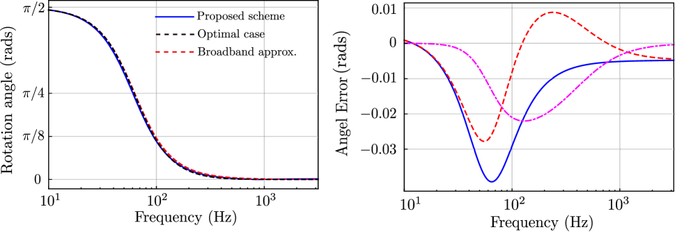
Figure 6: Left panel: Rotation angle for the $\hat{b}-$ field. The blue curve is the result computed using the parameters given in Tab.1 of the main text and exact transfer matrix technique. The red dashed curve is the optimal result of $\Phi_{\rm rot}=-{\rm arctan}\mathcal{K}$ while the green dashed curve is the rotation angle when we approximate $\mathcal{K}$ using broadband approximation as discussed in the main text of this supplementary material. Right panel: Error of the rotation angle. (1)The magenta dotdashed curve is the difference between the analytical result of rotation angle under broadband approximation and the optimal angle ; (2) the blue curve is the difference between the rotation angle computed from our proposed scheme and the analytical result under broadband approximation; (3) the red dashed curve is the difference between the rotation angle computed from our proposed scheme and the optimal analytical result.

IV Loss analysis

Fig.3 of the main text takes into account of the loss in our system. There are four main loss sources in our design: (1) the loss due to the arm cavity and signal recycling cavity, which currently has the value round $100$ ppm (per round trip) and $2000$ ppm (per round trip) and has a small effect on the noise, compare to the current filter cavity design which has the value around $1$ppm per meter. (2) the input loss comes from the loss of the optical devices in the input optical path and mode mismatch and the readout loss comes from the measurement channel due to the non-perfect quantum efficiency of the photo-detector and the lossy optical devices in the output optical path and also mode mismatch. (3) The phase fluctuation of the local oscillators which are used to measure the $\hat{a}$ and $\hat{b}-$fields.

IV.1 Arm cavity loss and signal recycling cavity loss

Similar to what has been discussed in [6], for the signal channel, $100$ ppm round trip loss in the arm cavity corresponds to about 0.3% total loss (considering the circulation of light fields) in advanced LIGO since it works in the resonant sideband extraction mode, which is comparabl to the impact of signal recycling cavity loss ($\sim 0.2\%$) at the interesting frequency band. However, since the large detuned idler field does not resonant with the signal recycling cavity, thereby a more careful simulation is needed. We simulate the effects of these noises in the following Fig. 7 to compare the impact of these different noise sources (a similar figure was also shown in [6]). Note that at low frequency, the impact of these noises on the idler channel is much less than that on the signal channel, since idler field does not drive the interferometer mirrors through radiation pressure force noise in the interested frequency domain.

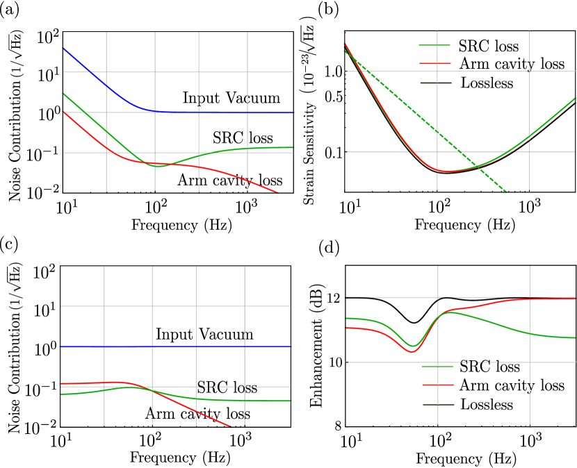
Figure 7: Simulation of quantum noise contributions from the arm and signal recycling cavities (round trip losses $\epsilon_{c}=100$ ppm and $\epsilon_{\rm SRC}=2000$ ppm respectively, as in the main text) and their impact on strain sensitivity and sensitivity enhancement. (a) Signal channel: comparison of quantum noise contributions in the signal channel from (unsqueezed) vacuum fluctuations, arm cavity loss, and SRC loss. The noise fields beat with a strong carrier field, resulting in radiation pressure noise below 50 Hz due to the ponderomotive effect. (b) Idler channel: comparison of contributions in the idler channel from (unsqueezed) vacuum fluctuations, arm cavity loss, and SRC loss. The noise fields do not beat with a strong carrier field, and therefore do not participate in the ponderomotive process. (c) The (small) impact of loss due to combined signal and idler channels, shown separately for arm cavity loss and SRC loss (d) Impact of cavity losses on sensitivity enhancement due to the proposed conditioning scheme.

IV.2 Input Loss and readout loss

Let us now investigate the effect of the input loss and the readout loss. The sensitivity curve in Fig. 3 of the main text is computed using numerical transfer-matrix approach [8]. Here for giving an analytical formula, we apply the single-mode approximation which is a very good approximation within one free-spectral-range of the arm cavity. The exact results about the contribution from the input loss and readout loss respectively are shown in Fig. 8. Since the $\hat{a}$ and $\hat{b}$ fields propagate in a collinear way and share the same optical mode, therefore the input and readout loss of the $\hat{a}$ and $\hat{b}-$fields are the same, denoted by $\epsilon_{\rm in}$ (in terms of power) and we have:

$$\hat{a}\rightarrow\sqrt{1-\epsilon_{\rm in}}\hat{a}+\sqrt{\epsilon_{\rm in}}\hat{n}^{\rm in}_{s},\quad\hat{b}\rightarrow\sqrt{1-\epsilon_{\rm in}}\hat{b}+\sqrt{\epsilon_{\rm in}}\hat{n}^{\rm in}_{i},$$ (35)

$$\hat{A}_{2}\rightarrow\sqrt{1-\epsilon_{r}}\hat{A}_{2}+\sqrt{\epsilon_{r}}\hat{n}^{r}_{s},\quad\hat{B}_{2}\rightarrow\sqrt{1-\epsilon_{r}}\hat{B}_{2}+\sqrt{\epsilon_{r}}\hat{n}^{r}_{i}.$$ (36)

where $\hat{n}^{\rm in}_{s}$ and $\hat{n}^{\rm in}_{i}$ are two uncorrelated injection noises and $\hat{n}^{r}_{s}$ and $\hat{n}^{r}_{i}$ are two uncorrelated readout noises associated with two homodyne detectors.

Expand to the first order of $\epsilon_{\rm in}$ and $\epsilon_{r}$, we have the approximated formula for the degradation of the strain sensitivity as a summation of input loss contribution $\Delta S^{\epsilon_{\rm in}\rm cond}_{\rm hh}$ and the readout loss contribution $\Delta S^{\epsilon_{r}\rm cond}_{\rm hh}$:

$$\Delta S_{\rm hh}^{\epsilon\rm cond}=\Delta S^{\epsilon_{\rm in}\rm cond}_{\rm hh}+\Delta S^{\epsilon_{r}\rm cond}_{\rm hh}$$ (37)

where:

$$\Delta S^{\epsilon_{\rm in}\rm cond}_{\rm hh}\approx\frac{h_{\rm SQL}^{2}}{2\cosh{2r}}\left(\mathcal{K}+\frac{1}{\mathcal{K}}\right)\left(\frac{2\cosh{2r}^{2}-\cosh{2r}-1}{\cosh{2r}}\right)\epsilon_{\rm in}$$ (38)

$$\Delta S^{\epsilon_{r}\rm cond}_{\rm hh}\approx\frac{h_{\rm SQL}^{2}}{2}\left(\mathcal{K}\tanh^{2}{2r}+\frac{1+\tanh^{2}{2r}}{\mathcal{K}}\right)\epsilon_{r}.$$ (39)

It is easy to see that the effect of the input loss contributes a broadband degradation of squeezing degree. This degradation is frequency independent. However, for the readout loss, at high frequencies where $\mathcal{K}\ll 1$ the relative loss correction is roughly $\Delta S^{\epsilon_{r}\rm cond}_{\rm hh}/S_{\rm hh}^{\rm cond}\approx[1+(\tanh{2r})^{2}]\epsilon_{r}$, while at low frequencies where $\mathcal{K}\gg 1$, $\Delta S^{\epsilon_{r}\rm cond}_{\rm hh}/S_{\rm hh}^{\rm cond}$ is roughly $(\tanh{2r})^{2}\epsilon_{r}$. Therefore the readout loss effect at high frequencies is higher than that at low frequencies, due to the fact that the pondermotive effect amplifies the signal at the low frequency band [2]. This character of the sensitivity curves has been shown in Fig. 3 of the main text and more explicitly in Fig. 8 of this Supplementary Material.

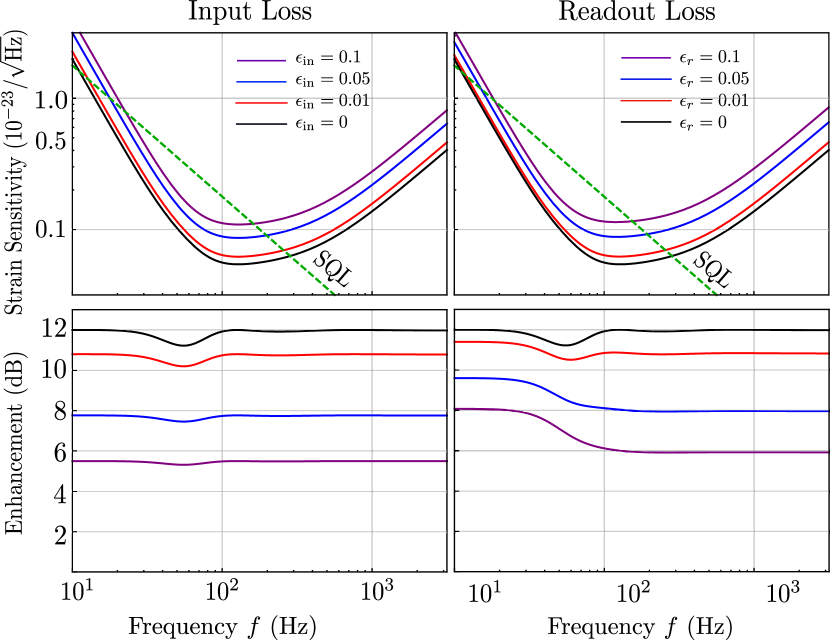
Figure 8: Left panel: the strain sensitivity and enhancement factor of our configuration when there is only input loss. Right panel: the strain sensitivity and enhancement factor of our configuration when there is only readout loss.

If we take the assumption of $\epsilon_{\rm in}=\epsilon_{r}=\epsilon$, the noise spectrum for the traditional broadband squeezing using an additional filter cavity and the conditional squeezing, including the loss $\epsilon$ to the first order, and under the approximation that the squeezing degree is large, we have:

$$\Delta S_{\rm hh}^{\epsilon\rm cond}\approx\frac{h_{\rm SQL}^{2}}{2}\left(\frac{2}{\mathcal{K}}+\frac{3}{2}\mathcal{K}\right)2\epsilon,\quad\Delta S_{\rm hh}^{\epsilon\rm tran}\approx\frac{h_{\rm SQL}^{2}}{2}\left(\frac{2}{\mathcal{K}}+\mathcal{K}\right)\epsilon,$$ (41)

where $\Delta S_{\rm hh}^{\epsilon\rm tran}$ is the first order correction to the sensitivity curve produced by traditional squeezing scheme [2, 7] and clearly we have $\Delta S_{\rm hh}^{\epsilon\rm cond}\approx 2\Delta S_{\rm hh}^{\epsilon\rm tran}$. As we have briefly mentioned in the main text, due to the fact that both signal and idler beams experience the same loss during their propagation in our scheme, the input and readout losses in our configuration are roughly doubled compare to that of the traditional squeezing scheme with an additional filter cavity.

IV.3 Phase fluctuation

The classical phase uncertainty of local oscillators in homodyne detection scheme has a very small effect on the sensitivity, proved as follows.

We assume that the phase fluctuation of the local oscillators used for signal and idler detection are independent Gaussian random variables represented by $\xi_{s}$ and $\xi_{i}$ respectively, with zero mean and standard variacne $\xi_{vs}$ and $\xi_{vi}$, such that their probability density functions are given by:

$$P_{s}(\xi_{s})=\frac{1}{\sqrt{2\pi\xi_{vs}^{2}}}e^{-\frac{\xi_{s}^{2}}{2\xi_{vs}^{2}}},\quad P_{i}(\xi_{i})=\frac{1}{\sqrt{2\pi\xi_{vi}^{2}}}e^{-\frac{\xi_{i}^{2}}{2\xi_{vi}^{2}}},$$ (42)

For measuring any field $\hat{O}$, the effect of phase fluctuation $\xi_{O}$ in a phase quadrature readout scheme is that the actual detected quadrature is also a random variable which is given by $\hat{O}_{m}(t)=-\hat{O}_{1}(t)\sin{\xi_{O}}+\hat{O}_{2}(t)\cos{\xi_{O}}$. The ensemble-averaged variance of the detected quadrature is then [9]:

$$\begin{split}S_{\hat{O}_{m}\hat{O}_{m}}&=\frac{1}{2}\int d\xi_{O}P(\xi_{O})\langle\hat{O}_{m}\hat{O}_{m}^{\dagger}+\hat{O}_{m}^{\dagger}\hat{O}_{m}\rangle\\ &=V_{\hat{O}_{1}\hat{O}_{1}}\int d\xi_{O}P(\xi_{O})\sin\xi_{O}^{2}+V_{\hat{O}_{2}\hat{O}_{2}}\int d\xi_{O}P(\xi_{O})\cos\xi_{O}^{2}+(V_{\hat{O}_{1}\hat{O}_{2}}+V_{\hat{O}_{2}\hat{O}_{1}})\sin\xi_{O}\cos\xi_{O}\\ \end{split}$$ (43)

Now if we use the identities (we assume that $\xi_{vo}\ll 1$.):

$$\begin{split}&\int d\xi_{O}P(\xi_{O})\sin^{2}\xi_{O}=e^{-\xi_{ov}^{2}}\sinh{\xi_{ov}^{2}}\approx\xi_{ov}^{2}\approx\sin{\xi_{ov}^{2}}\\ &\int d\xi_{O}P(\xi_{O})\cos^{2}\xi_{O}=e^{-\xi_{ov}^{2}}\cosh{\xi_{ov}^{2}}\approx 1-\xi_{ov}^{2}\approx\cos{\xi_{ov}^{2}},\end{split}$$ (44)

and the fact that the $\sin\xi_{O}\cos\xi_{O}$ is an odd function, one can obtain:

$$S_{\hat{O}_{m}\hat{O}_{m}}\approx\cos{\xi_{vo}^{2}}V_{\hat{O}_{1}\hat{O}_{1}}+\sin{\xi_{vo}^{2}}V_{\hat{O}_{2}\hat{O}_{2}}.$$ (45)

Using the above formula, one can can compute the variance of signal and idler fields.

Similarly, the cross correlation between the signal and idler fields (represented by $\hat{A}$ and $\hat{B}$) in the phase quadrature readout scheme, accounting for phase fluctuations, is given by:

$$S_{A_{m}B_{m}}=\frac{1}{2}\int d\xi_{i}d\xi_{s}P(\xi_{i})P(\xi_{s})\langle(\hat{A}_{1}\sin\xi_{s}+\hat{A}_{2}\cos\xi_{s})(\hat{B}_{1}\cos\xi_{i}+\hat{B}_{2}\sin\xi_{i})\rangle.$$ (46)

Because $\xi_{i}$ and $\xi_{s}$ are two independent random variables, the above cross correlation fluctuation leads to:

$$S_{A_{m}B_{m}}=S_{A_{2}B_{1}}e^{-\frac{\xi_{vs}^{2}+\xi_{vi}^{2}}{2}}\approx S_{a_{2}b_{1}}\left(1-\frac{\xi_{vs}^{2}+\xi_{vi}^{2}}{2}\right).$$ (47)

where we have used the identities:

$$\int d\xi_{O}P(\xi_{O})\cos\xi_{O}=e^{-\frac{\xi_{O}^{2}}{2}},\quad\int d\xi_{O}P(\xi_{O})\sin\xi_{O}=0.$$ (48)

Substituting Eq. (45) and Eq. (47) into Eq. (18), the final strain sensitivity can be written as:

$$\begin{split}S_{hh}=\frac{h_{\rm SQL}^{2}}{2\cosh{2r}}\left[\frac{1+(\xi_{vs}^{2}+\xi_{vi}^{2})\sinh{4r}}{\mathcal{K}}+(1-\xi_{vs}^{2}+\xi_{vi}^{2}\sinh{4r})\mathcal{K}\right].\end{split}$$ (49)

The typical experimental rms of the local oscillator phase is taken to be $1.7$m rad such as shown in [10], that means the phase fluctuation quantities in the above formula have an orders of magnitude $\sim 10^{-6}$ rad². For a 15dB squeezer, $1$ mrad phase jittering only contributes roughly $\sim 0.5\%$ relative correction to the final sensitivity.

References

- [1] B. Abbott (et al.). Observation of Gravitational Waves from a Binary Black Hole Merger. Phys. Rev. Lett, 116(061102), 2016.
- [2] M. Punturo (et al.). The Einstein Telescope: a third-generation gravitational wave observatory. Classical and Quantum Gravity, 27(19), 2010.
- [3] S. Danilishin and F. Ya. Khalili. Quantum Measurement Theory in Gravitational-Wave Detectors. Living Rev. Relativity, 15(5), 2012.
- [4] H. Miao, H. Yang, R. X. Adhikari, and Y. Chen. Quantum limits of interferometer topologies for gravitational radiation detection. Classical Quantum Gravity, 31(16), August 2014.
- [5] S. Dwyer, D. Sigg, S. Ballmer, L. Barsotti, N. Mavalvala, and M. Evans. Gravitational wave detector with cosmological reach. Phys. Rev. D, 91(082001), 2015.
- [6] B. Abbott (et al.). Exploring the sensitivity of next generation gravitational wave detectors. LIGO Document, (P1600143-v14), 2016.
- [7] B. Sathyaprakash (et. al). Scientific objectives of Einstein Telescope. Classical and Quantum Gravity, 29(12), 2012.
- [8] R. Tso, M. Isi, Y. Chen, and L. Stein. Modeling the dispersion and polarization content of gravitational waves for tests of general relativity. In Seventh Meeting on CPT and Lorentz Symmetry, June 2016.
- [9] A. Kostelecky and M. Mewes. Testing local Lorentz invariance with gravitational waves. Phys. Lett. B, 757:510–514, 2016.
- [10] Lasky, E. Thrane, Yu. Levin, J. Blackman, and Y. Chen. Detecting gravitational-wave memory with ligo: implications of gw150914. Phys. Rev. Lett, 117(061102), 2016.
- [11] E. Berti. Astrophysical Black Holes as Natural Laboratories for Fundamental Physics and Strong-Field Gravity. Braz J Phys, 43(341), 2013.
- [12] Q. Chu, E. J. Howell, A. Rowlinson, H. Gao, B. Zhang, S. J. Tingay, M. Boër, and L. Wen. Capturing the electromagnetic counterparts of binary neutron star mergers through low-latency gravitational wave triggers. MNRAS, 459:121–139, Jun 2016.
- [13] B. D. Metzger and E. Berger. What is the most promising electromagnetic counterpart of a neutron star binary merger? The Astrophysical Journal, 746(1):48, 2012.
- [14] J. Aasi(et. al). Constraints on Cosmic Strings from the LIGO-Virgo Gravitational-Wave Detectors. Phys. Rev. Lett, 112(131101), 2014.
- [15] R. W. P. Drever, J. Hough, W. A. Edelstein, J. R. Pugh, and W. Martin. In B. Bertotii, editor, Experimental Gravitation, page 365, Pavia, Italy., 1976. Accademia Nazionale dei Lincei.
- [16] V. B Braginsky and Yu. I. Vorontsov. Usp. Fiz. Nauk, 114(41), 1974.
- [17] R. Weiss. Sources of Gravitational Radiation. Cambridge University Press, 1979.
- [18] C. M. Caves. Quantum-mechanical noise in an interferometer. Phys. Rev. D, 23(1693), April 1981.
- [19] H. J. Kimble, Yu. Levin, A. B. Matsko, K. S. Thorne, and S. P. Vyatchanin. Conversion of conventional gravitational-wave interferometers into quantum nondemolition interferometers by modifying their input and/or output optics. Phys. Rev. D, 65(022002), 2001.
- [20] A. Buonanno and Y. Chen. Quantum noise in second generation, signal-recycled laser interferometric gravitational-wave detectors. Phys. Rev. D, 64(042006), 2001.
- [21] A. Buonanno and Y. Chen. Scaling law in signal recycled laser-interferometer gravitational-wave detectors. Phys. Rev. D, 67(062002), 2003.
- [22] W. G Unruh. Quantum Noise in the Interferometer Detector, page 647. Plenum Press, New York, 1983.
- [23] R. Schnabel, N. Mavalvala, D. E. McClelland, and P. K. Lam. Quantum metrology for gravitational wave astronomy. Nat. Commun., 1(121), 2010.
- [24] LIGO Instrument Science White Paper. Technical report, Feb. 2015.
- [25] H. Vahlbruch, M. Mehmet, S. Chelkowski, B. Hage, A. Franzen, N. Lastzka, S. Gossler, K. Danzmann, and R. Schnabel. Observation of Squeezed Light with 10-dB Quantum-Noise Reduction. Phys. Rev. Lett, 100(033602), 2009.
- [26] M Mehmet, S. Ast, T. Eberle, S. Steinlechner, H. Vahlbruch, and R. Schnabel. Squeezed light at 1550 nm with a quantum noise reduction of 12.3 dB. Optics Express, 19(25763), 2011.
- [27] S. S. Y. Chua, M. S. Stefszky, C. M. Mow-Lowry, B. C. Buchler, S. Dwyer, D. A. Shaddock, P. K. Lam, and D. E. McClelland. Backscatter tolerant squeezed light source for advanced gravitational-wave detectors. Optics Letters, 36(23):4680–4682, 2011.
- [28] M. S. Stefszky, C. M. Mow-Lowry, S. S. Y. Chua, D. A. Shaddock, B. C. Buchler, H. Vahlbruch, A. Khalaidovski, R. Schnabel, P. K. Lam, and D. E. McClelland. Balanced homodyne detection of optical quantum states at audio-band frequencies and below. Classical Quantum Gravity, 29(145015), 2012.
- [29] K. McKenzie, N. Grosse, W. P. Bowen, S. E. Whitcomb, M. B. Gray, D. E. McClelland, and P. K. Lam. Squeezing in the Audio Gravitational-Wave Detection Band. Phys. Rev. Lett, 93(161105), 2004.
- [30] H. Vahlbruch, M. Mehmet, K. Danzmann, and R. Schnabel. Detection of 15 dB squeezed states of light and their application for the absolute calibration of photo-electric quantum efficiency. Phys. Rev. Lett (accepted), 2016.
- [31] B. Abbott (et al.). A gravitational wave observatory operating beyond the quantum shot-noise limit. Nature Physics, 7(962), 2011.
- [32] B. Abbott (et al.). Enhanced sensitivity of the LIGO gravitational wave detector by using squeezed states of light. Nature Photonics, 7(613), 2013.
- [33] M. T. Jaekel and S. Reynaud. Quantum Limits in Interferometer Measurement. EPL (Europhysics Letters), 13(4):301, 1990.
- [34] S. Chelkowski, H. Vahlbruch, B. Hage, A. Franzen, N. Lastzka, K. Danzmann, and R. Schnabel. Experimental characterization of frequency-dependent squeezed light. Phys. Rev. A, 71(013806), 2005.
- [35] M. Evans, L. Barsotti, P. Kwee, J. Harms, and H. Miao. Realistic filter cavities for advanced gravitational wave detectors. Phys. Rev. D, 88(022002), 2013.
- [36] F. Ya. Khalili. Quantum variational measurement in the next generation gravitational-wave detectors. Phys. Rev. D, 76(102002), 2007.
- [37] F. Ya. Khalili. Optimal configurations of filter cavity in future gravitational-wave detectors. Phys. Rev. D, 81(122002), 2010.
- [38] T. Isogai, J. Miller, P. Kwee, L. Barsotti, and M. Evans. Loss in long-storage-time optical cavities. Optics Express, 21(24):30114–30125, 2013.
- [39] P. Kwee, J. Miller, T. Isogai, L. Barsotti, and M. Evans. Decoherence and degradation of squeezed states in quantum filter cavities. Phys. Rev. D, 90(062006), 2014.
- [40] E Caposcasa, M Barsuglia, J Degallaix, L Pinard, N. Straniero, R. Schnabel, K. Somiya, Y. Aso, D. Tatsumi, and R. Flaminio. Estimation of losses in a 300 m filter cavity and quantum noise reduction in the kagra gravitational-wave detector. Phys. Rev. D, 93(082004), 2016.
- [41] ET Science Team. Einstein gravitative wave telescope conceptual design study. ET-0106C-10, 2011.
- [42] E. E. Mikhailov, K. Goda, T. Corbitt, and N. Mavalvala. Frequency-dependent squeeze-amplitude attenuation and squeeze-angle rotation by electromagnetically induced transparency for gravitational-wave interferometers. Phys. Rev. A, 73(053810), 2006.
- [43] Y. Ma, S. L. Danilishin, C. Zhao, H. Miao, W. Z. Korth, Y. Chen, R. L. Ward, and D. G. Blair. Narrowing the Filter-Cavity Bandwidth in Gravitational-Wave Detectors via Optomechanical Interaction. Phys. Rev. Lett, 113(151102), 2014.
- [44] J Qin, C Zhao, Y Ma, X Chen, L Ju, and D. G. Blair. Classical demonstration of frequency-dependent noise ellipse rotation using optomechanically induced transparency. Phys. Rev. A, 89(041802(R)), 2014.
- [45] J. Zhang. Einstein-Podolsky-Rosen sideband entanglement in broadband squeezed light. Phys. Rev. A, 67(054302), 2003.
- [46] A. M Marino, C. R Stroud, V Wong, R. S Bennink, and R. W. Boyd. Bichromatic local oscillator for detection of two-mode squeezed states of light. J. Opt. Soc. Am. B, 24(2):335–339, 2007.
- [47] B. Hage, A. Samblowski, and R. Schnabel. Towards Einstein-Podolsky-Rosen quantum channel multiplexing. Phys. Rev. A, 81(062301), June 2010.
- [48] L. Barsotti. Ligo: The A+ Upgrade. LIGO Document, (G1601199-v2), 2016.
- [49] L. Barsotti. Squeezing for Advanced LIGO. LIGO Document, G1401092-v1, 2014.

References

- [1] M. O. Scully and M. S. Zubairy. Quantum Optics (Chapter 16). Cambridge University Press, 1997.
- [2] H. J. Kimble, Yu. Levin, A. B. Matsko, K. S. Thorne, and S. P. Vyatchanin. Conversion of conventional gravitational-wave interferometers into quantum nondemolition interferometers by modifying their input and/or output optics. Phys. Rev. D, 65(022002), 2001.
- [3] P. Purdue and Y. Chen. Practical speed meter designs for quantum nondemolition gravitational-wave interferometers. Phys. Rev. D, 66(122004), 2002.
- [4] F. Ya. Khalili. Quantum variational measurement in the next generation gravitational-wave detectors. Phys. Rev. D, 76(102002), 2007.
- [5] A. Buonanno and Y. Chen. Scaling law in signal recycled laser-interferometer gravitational-wave detectors. Phys. Rev. D, 67(062002), 2003.
- [6] L. Barsotti. Squeezing for Advanced LIGO. LIGO Document, G1401092-v1, 2014.
- [7] H. Miao, H. Yang, R. X. Adhikari, and Y. Chen. Quantum limits of interferometer topologies for gravitational radiation detection. Classical Quantum Gravity, 31(16), August 2014.
- [8] T. Corbitt, Y. Chen, and N. Mavalvala. Mathematical framework for simulation of quantum fields in complex interferometers using the two-photon formalism. Phys. Rev. A, 72(013818), July 2005.
- [9] T. Aoki, G. Takahashi, and A Furusawa. Squeezing at 946nm with periodically poled KTiOPO4. Opt. Express, 14(15):6930–6935, 2006.
- [10] H. Vahlbruch, M. Mehmet, K. Danzmann, and R. Schnabel. Detection of 15 db squeezed states of light and their application for the absolute calibration of photo-electric quantum efficiency. Phys. Rev. Lett (accepted), 2016.