Three-dimensional Simulations of AGN Jets: Magnetic Kink Instability versus Conical Shocks

Abstract

Relativistic jets in active galactic nuclei (AGN) convert as much as half of their energy into radiation. To explore the poorly understood processes that are responsible for this conversion, we carry out fully 3D magnetohydrodynamic (MHD) simulations of relativistic magnetized jets. Unlike the standard approach of injecting the jets at large radii, our simulated jets self-consistently form at the source and propagate and accelerate outward for several orders of magnitude in distance before they interact with the ambient medium. We find that this interaction can trigger strong energy dissipation of two kinds inside the jets, depending on the properties of the ambient medium. Those jets that form in a new outburst and drill a fresh hole through the ambient medium fall victim to a 3D magnetic kink instability and dissipate their energy primarily through magnetic reconnection in the current sheets formed by the instability. On the other hand, those jets that form during repeated cycles of AGN activity and escape through a pre-existing hole in the ambient medium maintain their stability and dissipate their energy primarily at MHD recollimation shocks. In both cases the dissipation region can be associated with a change in the density profile of the ambient gas. The Bondi radius in AGN jets serves as such a location.

1 Introduction

Black holes (BHs) reprocess infalling gas into outflows and radiation. Of particular importance are relativistic collimated outflows, which we will refer to simply as jets. Relativistic motions have been inferred in various astrophysical systems including long- and short-duration gamma-ray bursts (GRBs, e.g., Frail et al., 2001; Panaitescu & Kumar, 2002; Taylor et al., 2004), active galactic nuclei (AGN, e.g., Biretta, Sparks & Macchetto 1999; Jorstad et al. 2005; Lister et al. 2011; Meyer et al. 2013), and black hole X-ray binaries (e.g., Fender, Belloni & Gallo, 2004). The relativistic motion of jets implies that they start out highly magnetized, with very few baryons (otherwise they would have insufficient power to accelerate to the observed Lorentz factors), and are likely powered by the rotation of the central supermassive BHs (e.g., Tchekhovskoy, Narayan & McKinney, 2011). Observationally, jet power is comparable to the accretion power (Rawlings & Saunders, 1991; Ghisellini et al., 2014; Nemmen & Tchekhovskoy, 2015), suggesting that the jets are an energetically important component of the system. Indeed, jets can affect the evolution of BHs and their host galaxies, e.g., via extracting the black hole spin energy (e.g., Gammie, Shapiro & McKinney, 2004; Tchekhovskoy, 2015), heating the ambient gas and suppressing its infall, with important implications for the cooling flow problem in the context of galaxy clusters and star formation (e.g., Vernaleo & Reynolds, 2006; Ishibashi & Fabian, 2012; Gaspari, Ruszkowski & Sharma, 2012; Li et al., 2015; Fielding et al., 2016).

Even though jets are widely thought to be powered at least in part by magnetic fields, most studies of the dissipation zone (i) assume axisymmetry or ignore magnetic fields (e.g., Aloy et al., 2000; Morsony, Lazzati & Begelman, 2007; Vernaleo & Reynolds, 2007; Rossi et al., 2008; Meliani, Keppens & Giacomazzo, 2008; Perucho et al., 2010; Yoon et al., 2011; Kohler, Begelman & Beckwith, 2012; De Colle et al., 2012; López-Cámara et al., 2013; Mizuno et al., 2015), (ii) prescribe jet injection at large distances (e.g., Nakamura, Li & Li, 2007; Mignone et al., 2010, 2013; Guan, Li & Li, 2014), or (iii) consider a segment of a pre-existing jet (Mizuno et al., 2012; Mizuno, Hardee & Nishikawa, 2014; Porth & Komissarov, 2015; Singh, Mizuno & de Gouveia Dal Pino, 2016). Assumption (i) ignores known 3D magnetic instabilities, the most serious of which is the magnetic kink instability (e.g. Begelman, 1998; Lyubarskii, 1999; Narayan, Li & Tchekhovskoy, 2009), which can result in the dissipation trigger for the jet radiation (e.g., Begelman, 1998; Nakamura & Meier, 2004; Giannios & Spruit, 2006) or can even globally disrupt the jets (Tchekhovskoy & Bromberg, 2016). Assumption (ii) breaks the self-consistent connection of the jets to the central engine and prevents them from establishing a natural value of the magnetic pitch, or the ratio of poloidal and toroidal magnetic field strength, that is crucial for jet stability as we discuss below (see also Bromberg & Tchekhovskoy, 2016). Assumption (iii) considers a segment of the jets and limits the ability to address global jet stability properties.

Indeed, jets propagate through a vast range of distances from the event horizon of the BH ($\sim 10^{-7}[M_{\rm BH}/10^{9}M_{\odot}]$ kpc, where $M_{\rm BH}$ is the black hole mass) to outside the galaxy ($\sim 10^{3}$ kpc), giving wide latitude — ten orders of magnitude in distance — for magnetic instabilities to develop. Along the way, the jets radiate as much as 10–50% of their luminosity as photons at characteristic scales, where major dissipation events take place (the “dissipation zone”), such as the blazar zone and the knots in AGN and the prompt emission in GRBs (e.g., Panaitescu & Kumar, 2002; Nemmen et al., 2012; Ghisellini et al., 2014). The cause of energy dissipation is actively debated. It can be triggered by internal processes (e.g., internal shocks, MHD instabilities) and external interactions (e.g., recollimation shocks, external shocks), or the interplay between the two. Since, within the MHD paradigm, jets are expected to reach the dissipation zone magnetically dominated, dissipation of magnetic energy is the most likely source of jet radiation (e.g., Spruit, Daigne & Drenkhahn, 2001; Lyutikov & Blandford, 2003; Narayan, Kumar & Tchekhovskoy, 2011; Sironi, Petropoulou & Giannios, 2015).

In this paper, we study the effect of the external medium on the jet dissipation zone using relativistic magnetohydrodynamic (MHD) simulations. In order to capture the development of non-axisymmetric magnetic instabilities, we include magnetic fields and carry out the simulations in full 3D. We also consider the launching of the jet essentially from the surface of the central compact object. With our approach, the magnetic pitch at the base of the jet is at its natural value self-consistently set by the rotation of the central object, instead of being chosen a priori. Because the magnetic pitch controls jet stability to the 3D magnetic kink (Appl, Lery & Baty, 2000; Narayan, Li & Tchekhovskoy, 2009; Guan, Li & Li, 2014), our approach allows us to study the stability of relativistic jets from first principles.

Kink instability in a magnetized jet is similar to that in a spring: the spring flies sideways as we squeeze it. Whether the jet is susceptible to the kink instability depends on whether the instability has enough time to grow. If the instability growth time-scale is shorter than the time it takes for the fluid to travel from the base to the tip of the jet, the jet will become unstable. If the jet is strongly compressed and therefore toroidally-dominated, the instability grows faster. And because jet compression is determined by the interaction with the ambient medium, the properties of the ambient medium that the jet propagates through can have a profound effect on jet stability (Bromberg & Tchekhovskoy, 2016). In a new outburst, a jet drills a hole through the “pristine” ambient medium and develops a highly pressurized region at the tip of the jet – the jet head – that does the drilling and pushes the ambient medium out of the way. We refer to such jets as headed jets. The push against the external medium compresses the headed jets into a tighter magnetic helix. This increases their toroidal magnetic pressure and destabilizes them against the 3D magnetic kink instability (Bromberg & Tchekhovskoy, 2016). A more lucky jet, for which a hole was pre-drilled along the jet propagation path by previous AGN activity and has not had the time to close, does not develop a head. We refer to such jets as headless jets; they tend to be more stable. For instance, 3D simulations of such jets did not find significant dissipation due to 3D instabilities (Hawley & Krolik, 2006; McKinney & Blandford, 2009; Tchekhovskoy, Narayan & McKinney, 2011).

The distinction between the two types of jets is not always clear-cut. For instance, short-GRB jets, believed to be produced by compact binary mergers, could initially be headless but eventually run into the material ejected early in the merger process (e.g., Murguia-Berthier et al., 2014) and develop instabilities. Conversely, core-collapse GRBs initially have to drill their escape route through the progenitor star, but once they emerge from it, they become headless. A clear picture of what determines the jet stability in general is still lacking. In this paper, we attempt to elucidate on this topic by clearly separating headless and headed jets and their interaction with the external medium.

The density profile of the ambient gas through which the jet propagates depends on the specifics of the astrophysical system. Here we use observations of jets in nearby AGN to guide us in including the effects of the ambient density into our models. Recent X-ray observations with Chandra inferred a shallow profile $\propto r^{-1}$, potentially accompanied by a jump, in the external medium profile of the M87 galaxy, near the edge of the central black hole’s sphere of influence, or the Bondi radius, $r_{\rm B}\sim 0.1$ kpc (Russell et al., 2015). Tchekhovskoy & Bromberg (2016) considered the interaction of uncollimated mildly relativistic jets with the external medium and hypothesized that this interaction starts around $r_{\rm B}$. To make their simulations computationally feasible, they initiated the jets at $r_{\rm B}$ and followed their propagation to galaxy scales, $\sim 10^{3}r_{\rm B}\sim 100$ kpc. However, by the time real jets reach $r_{\rm B}$, they are already well-collimated and move at relativistic velocities. For instance, the M87 jet collimates into a parabola (e.g., Nakamura & Asada, 2013 and references therein) and accelerates to Lorentz factors $\sim 6$ (e.g., Biretta, Sparks & Macchetto, 1999; Meyer et al., 2013) over $\sim 6$ orders of magnitude distance before it reaches $r_{\rm B}$. In this paper, we – for the first time – study the effects of acceleration and collimation of jets on their interaction with breaks, jumps, and other features in the ambient medium that are possibly present at $r_{\rm B}$.

As the first attempt to attack this 3D multi-scale problem of jet acceleration, collimation, and interaction with the ambient medium, we make several simplifications. We reduce the length of the acceleration zone down to $2$ orders of magnitude and consider jets of high-power (which propagate the fastest); we will also ignore gravity and assume a monopolar magnetic field geometry at the central compact object (see Sec. 2). In Section 2 we describe our numerical method and simulation setup. In Section 3 we present our simulation results for headed and headless jets. In Section 4 we discuss the astrophysical implications of our results and in Section 5 we conclude.

2 Simulation setup

We carry out time-dependent 3D relativistic MHD numerical simulations using the harm code (Gammie, McKinney & Tóth, 2003; Noble et al., 2006; Tchekhovskoy, McKinney & Narayan, 2007; McKinney & Blandford, 2009; Tchekhovskoy, Narayan & McKinney, 2011). We adopt a simulation setup inspired by Tchekhovskoy & Bromberg (2016); Bromberg & Tchekhovskoy (2016). We use modified spherical polar coordinates $(r,\theta,\varphi)$ and a numerical grid that spans the range $r_{\rm in}\leq r\leq r_{\rm out}$, $0\leq\theta\leq\pi$ and $0\leq\varphi\leq 2\pi$. All our simulations use $r_{\rm in}=r_{0}$, and $r_{\rm out}=10^{5}r_{\rm in}$. We initiate our jets at $r=r_{0}$, which is a few times the radius of the central compact object. So long as the jet is sub-Alfvenic at $r_{0}$, the value of $r_{0}$ does not affect the simulation outcome. Using a large value of $r_{\rm out}\gg r_{\rm in}$ ensures that the jets do not reach the outer boundary in a simulation time.

To isolate the intrinsically 3D effects, we will carry out both 2D and 3D simulations. In our 2D simulations the jets are pinned to the rotational axis by the axisymmetry, but in 3D they are free to deviate from the axis. Because of this, for our 2D simulations, we orient the rotational axis along the polar axis, $\theta=0$. However, for our 3D simulations, we direct the rotational axis along the $x$-axis, $\theta=\pi/2$, $\varphi=0$ (e.g., Moll, Spruit & Obergaulinger, 2008, see details in Bromberg & Tchekhovskoy, 2016) to allow complete freedom of 3D jet motion and avoid jet interaction with the polar singularity. For simplicity of presentation, when showing the results of both 2D and 3D simulations, regardless of the actual direction of the rotational axis, we will refer to it as the $z$-axis and orient it vertically in our figures.

Initially, we fill the domain with cold gas that we refer to as the “external density”, “ambient density” or simply “density”. We describe its spatial distribution below. The gas in our simulations is initially cold, apart from a very small amount of thermal energy supplied by the density “floors”, which have no effect on our results. Namely, if the values of density and/or internal energy drop below their floor values, $\rho_{\rm floor}=b^{2}/50$ and $u_{g,\rm floor}=b^{2}/250$ respectively, where $b$ is the total magnetic field strength in the fluid frame, we reset them to their floor values. The inner boundary is a perfectly conducting magnetized sphere. We will refer to it as the central object. We neglect gravity.

We thread the central object and the computational domain with a monopole (radial) magnetic field; using a dipole magnetic field produces similar jet properties (Bromberg & Tchekhovskoy, 2016). We fix the radial (normal) magnetic field strength of the central object and allow the other two magnetic field components to relax. The simulations start by instantaneously spinning up the sphere to a constant angular frequency $\Omega=0.8c/r_{\rm in}$. The electric field is zero in the frame instantaneously comoving with the sphere. The rotation coils up the initially radial magnetic field lines into helices and generates twin magnetized outflows from the surface of the central object that propagate mainly along the rotational axis. The rotation is uniform within $50^{\circ}$ of the rotational axis and smoothly goes to zero at $70^{\circ}$: this ensures that the twin outflows do not interact with the coordinate singularity. In other words, this ensures that in 3D there is no rotation of the central object at $\theta=0$, so there is no need to treat the boundary conditions at $\theta=0$ in any special way. The initial magnetization at the base of our jets is $\sigma_{0}=2p_{\rm mag,0}/\rho_{0}c^{2}\approx 25$, where $p_{\rm mag,0}=b_{0}^{2}/2$ is the magnetic pressure and $\rho_{0}$ is the density at the base of the jet. The initial internal energy of the jets is $u_{0}=p_{\rm mag,0}/62.5$. Thus, the initial plasma beta at the base of the jets is $\beta_{0}=(\gamma-1)u_{0}/p_{\rm mag,0}\approx 0.005\ll 1$, since the jet is cold, apart from a small amount of thermal energy supplied through the boundary conditions and the floors in our simulations solely for numerical stability purposes. This small amount of thermal energy has no effect on our results. Once the jets are launched by the rotation of the central compact object, they send a shock wave into the ambient medium. This blast wave heats up the ambient medium, and the thermal pressure of the medium confines and collimates the jets.

Our radial grid is uniformly spaced in $\log r$ out to a radius $10^{4}r_{\rm in}$, where the grid becomes progressively sparse. The angular grid is modified to concentrate the grid cells toward the rotational axis by following a parabolic shape $\delta\theta\propto r^{-\nu/2}$ (where $\delta\theta$ is measured away from the rotational axis), where we usually adopt $\nu=0.85$. The jets form and initially propagate along the rotational axis of the central object. In all figures, the central object is centred at the coordinate origin, $r=0$, and we will usually show only one jet that propagates from the center along the positive $z$-axis.

Model	Density	$\alpha$	$\beta$	$r_{t}/r_{0}$	$\chi$	$\delta$	$z_{0}/r_{0}$	$P_{\rm jet}$
name	(equation)							(${\rm erg\;s^{-1}}$)
A	(1)	3
A2	(2)	3	1	100	1			$10^{47}$
A2x3	(2)	3	1	100	3			$3\times 10^{46}$
A1	(2)	3	1	10	1			$10^{46}$
B	(5)	3				6
B2	(6)	3	1	100	3	6	80

Table 1: Initial ambient density profiles chosen for each of the simulations, according to equations (1)–(6), see Fig. 1. For simulations A2, A2x3 and A1 the density profile has a break at $r_{t}$, which we associate with the Bondi radius, $r_{\rm B}$. Using the M87 jet as a baseline, which has $P_{\rm jet}\approx 10^{44}$ erg/s, $r_{\rm B}\sim 0.1$ kpc and number density $n(r_{\rm B})\sim 1$ cm^-3 (e.g., Russell et al., 2015), we calculate a dimensionless parameter $\xi\equiv P_{\rm jet}/(n_{\rm B}m_{p}c^{3}r_{\rm B}^{2})$, where $m_{p}$ is the proton mass and $n_{\rm B}\equiv n(r_{\rm B})$ is the ambient number density at the Bondi radius. We compute the physical power of our simulated jets by scaling the simulated density at $r_{t}$ to the characteristic value, $n_{\rm B}=1\ {\rm cm}^{-3}$, while keeping the value of $\xi$ constant. All jet powers presented in this paper correspond to one jet.

3 Modelling jet interaction with the external medium

3.1 Headed Jets

3.1.1 Modeling the external medium

Relativistic jets are launched very close to the BH and are likely powered by the magnetized rotation of the BH. Jets accelerate as they collimate off the accretion disc wind (e.g., Beskin & Nokhrina, 2006; Komissarov et al., 2007; Tchekhovskoy, McKinney & Narayan, 2008). In this work, we focus on the asymptotic behaviour of the jets, and we would like to include the collimating effect of the accretion disc wind. In order to keep the simulation cost manageable, we opt to avoid the need to resolve the turbulent motions characteristic of the accretion disc. Because of this, we adopt a simplified approach that allows us to focus on the physics of the jets. To include the collimating effect of the accretion disc outflow, we immerse the central compact object into a spherically-symmetric ambient medium, with a power-law density profile,

$$\rho_{\rm A}=\rho_{0}\left(\displaystyle\frac{r}{r_{0}}\right)^{-\alpha}\qquad\text{(Model A).}$$ (1)

For our first model, which we refer to as model A, we choose the density distribution given by eq. (1) with a rather steep density profile, $\alpha=3$ (see Table 1 and the left panel of Fig. 1). The rapid drop off of density with distance roughly mimics the effect of the accretion disc wind. As we will see below, the ambient gas collimates the jet into a parabolic shape that resembles that inferred for the M87 jet (Asada & Nakamura, 2012) and 3D accretion disc–jet simulations (e.g., Hawley & Krolik, 2006; Tchekhovskoy, Narayan & McKinney, 2011). The steep density profile also allows the jet to accelerate to high velocities without having to cover a huge dynamical range, which is computationally expensive. This motivates our choice of $\alpha$. We carry out simulations of model A both in 2D and 3D, at different resolutions, as described in Tables 2 and 3. These tables also describe our simulation naming convention.

Naming	Resolution
convention	($N_{r}\times N_{\theta}\times N_{\phi}$)
X-2D	$256\times 96\times 1$
X-2D-hr	$512\times 192\times 1$
X-2D-vhr	$1024\times 384\times 1$
X-3D	$256\times 96\times 192$
X-3D-hr	$512\times 192\times 384$

Table 2: The naming convention we use for our simulations: “X” stands in for the model names followed by a “2D” or “3D” suffix denoting the dimensionality of the simulation and by an optional resolution suffix: “hr” for high resolution and “vhr” for very high resolution.

Model	Simulation	$t_{f}$
name	identifying suffix	$(r_{0}/c)$
A	-2D, -2D-hr, -2D-vhr, -3D	2700
A2	-2D, -2D-hr, -2D-vhr, -3D	3000
A2	-3D-hr	1500
A2x3	-2D, -2D-hr, -2D-vhr, -3D	3400
A1	-2D, -2D-hr, -2D-vhr, -3D	2800
B	-2D, -2D-hr, -2D-vhr, -3D	1500
B	-3D-hr	1200
B2	-2D, -2D-hr, -2D-vhr, -3D	2200
B2	-3D-hr	700

Table 3: List of the simulations we have carried out. Their names consist of a model name (left column) followed by a suffix (middle column). The simulations have been run until a time $t_{f}$ in units of $r_{0}/c$ (right column). We carried out a total of 27 different simulations. We give the parameters of each model in Table 1 and the resolution of our simulations in Table 2.

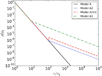
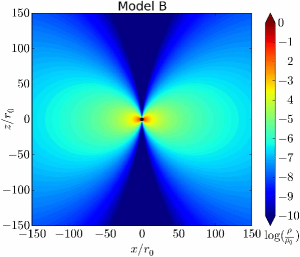
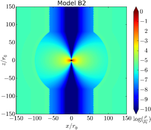
Figure 1: Models for the initial external medium we consider in this work. The left panel shows the density profiles in models A, which are spherically symmetric (see equations 1 and 2). The middle and right panels show density colour maps of $\log_{10}(\rho/\rho_{0})$ for models B and B2, respectively (see equations 5 and 6). The initial and boundary conditions of models B and B2 are axisymmetric (around the $z$-axis).

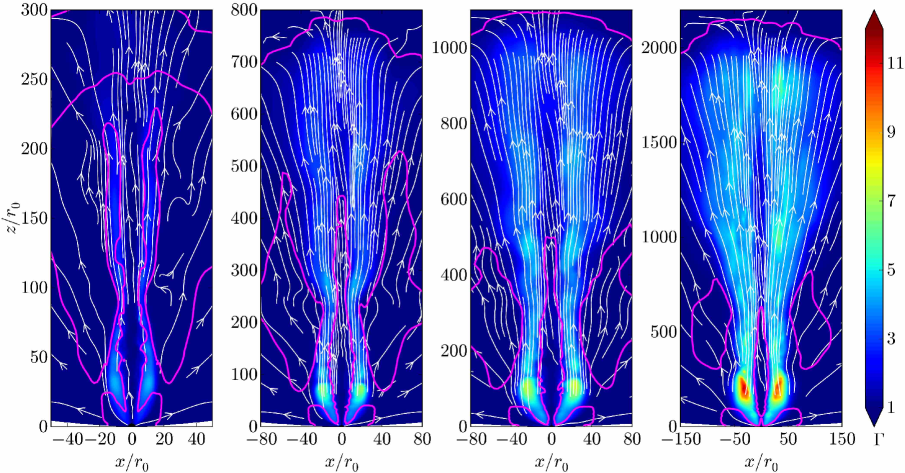
Figure 2: Cuts through the rotational axis of the Lorentz factor in our 3D simulation A-3D, at different times (from left to right, $t\approx 800r_{0}/c$, $t\approx 1300r_{0}/c$, $t\approx 1700r_{0}/c$ and $t\approx 2700r_{0}/c$; note different scales on the plots), with red (blue) colour showing high (low) values (please see the colour bar). The directed white lines show the velocity streamlines traced out in the image plane. In model A, the jet propagates into a density profile $\propto r^{-3}$. Throughout this work, we only show one jet propagating along the $z$-axis. The central compact object is located at $(0,0)$. The jet accelerates up to $\Gamma\sim 10$, as seen in the right panel. As the jet drills through the ambient medium it recollimates, which causes a drop in the Lorentz factor (seen at $z\sim 300r_{0}$ in the right panel). A weak recollimation point, initially at $z\sim 80r_{0}$ in the left panel, propagates outward at $\sim 0.3c$. This jet mostly retains its axisymmetry, indicating global stability against 3D magnetic kink modes. The magenta lines show the position of the fast magnetosonic surface. The jet (brightly coloured regions in these plots) accelerates to super-fast magnetosonic velocities by $z\sim 20r_{0}$. Therefore, information about any potential changes beyond this distance in the external medium cannot propagate back to the compact object, just as expected in AGN jets in nature.

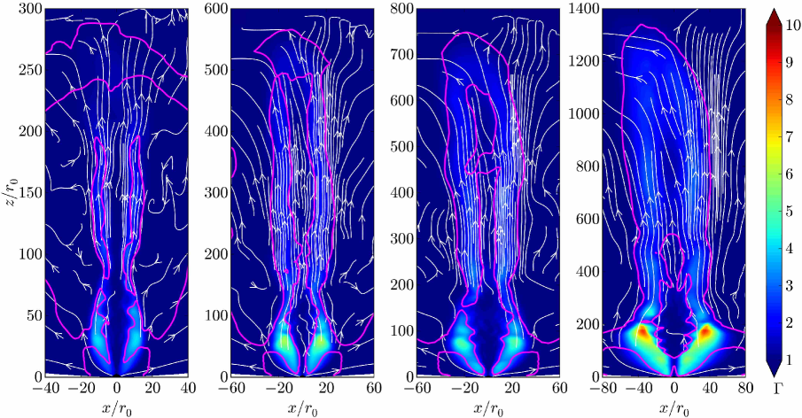
Figure 3: Cuts through the rotational axis of the Lorentz factor colour maps in our 3D simulation A2-3D, at different times (from left to right, $t\approx 800r_{0}/c$, $t\approx 1700r_{0}/c$, $t\approx 2200r_{0}/c$ and $t\approx 3000r_{0}/c$; note different scales on the plots, all panels share the same colorbar). The A2-3D jet runs into a density profile $\propto r^{-3}$ that flattens to $\propto r^{-1}$ at $100r_{0}$. This density break slows down the jet and makes the recollimation point (much more noticeable than in Fig. 2) move slower than in simulation A-3D. The magenta lines indicate the position of the fast magnetosonic surface and the white arrows show velocity streamlines. The jet velocity is super-fast magnetosonically beyond $z\sim 20r_{0}$: no information about the flattening in the density profile propagates back to the compact object. Unlike in the simulation A-3D without the density break, the A2-3D jet here shows strong deviations from axisymmetry. Thus, the density break tends to destabilize jets.

Fig. 2 shows a sequence of snapshots of our 3D simulation of model A, which we refer to as simulation A-3D (see Table 2). We show 2D colour maps of the jet Lorentz factor. When the jet runs into the ambient medium, which represents the accretion disc wind, it collimates. As the jet pushes the gas out of the way, the recollimation point (or the “pinch” of the jet) moves away from the center at $v\sim 0.3c$, reaching $z\sim 600r_{0}$ by $t=2700r_{0}/c$, as seen in the different panels of Fig. 2. The shape of the jet changes beyond the recolllimation point from parabolic-like to conical. As this sequence of snapshots shows, when presented with a continuous power-law density ambient medium, the jet self-similarly expands and does not show significant deviations from axisymmetry. The expansion causes the flow inside the recollimation point to accelerate, up to a Lorentz factor of $\Gamma\sim 10$, as seen in the right panel (the more the jet expands, the higher $\Gamma$ it reaches). Once the jet passes through the recollimation point, it slows down and the Lorentz factor drops down to $\Gamma\sim 5$.

The magenta lines in Fig. 2 show the position of the fast magnetosonic surface, or simply the fast surface. The jets start out moving at sub-fast magnetosonic velocity. However, as the jets expand and accelerate, they eventually outrun the fast waves, which happens at the fast surface located at $z\sim 20r_{0}$, as seen in the left panel of Fig. 2: beyond this distance, the fast waves can no longer communicate any information backwards. Because of this, when the jets undergo a recollimation or run into an obstacle in the ambient medium, this information is not communicated backwards along the jet. In fact, if the jet remained sub-fast throughout, then the information about any changes in the external medium could reach the central compact object and change the jet properties there. However, this would be an artefact of the reduced dynamic range of a simulation. In reality, since $r_{\rm B}$ is extremely far from the compact object, we expect the fast surface to be located at a distance well inside the Bondi radius. As we will see below, all our jets (except in model A1) accelerate to super-fast magnetosonic speeds before they encounter any changes in the external medium, as AGN jets do in nature.

As jets propagate outward in an AGN, they eventually encounter the ambient gas of the host galaxy. While it is generally uncertain how the radial profile of the accretion wind disc transitions to the interstellar medium (ISM) outside the sphere of influence of the black hole, X-ray observations of M87 (Russell et al., 2015) suggest a flattening of the density profile potentially accompanied with a factor of few jump in density, as we discuss below. Motivated by this, we model this transition via a break and a jump:

$$\rho=\begin{cases}\rho_{\rm A}(r)&r\leq r_{t}\\ \chi\left(\displaystyle\frac{r}{r_{t}}\right)^{-\beta}\rho_{\rm A}(r_{t})&r>r_{t},\end{cases}\qquad\text{(Model A\#)}$$ (2)

where the fiducial density profile $\rho_{\rm A}(r)$ is given by eq. (1), $r_{t}$ is the distance to the break in the density profile (from $\propto r^{-\alpha}$ to $\propto r^{-\beta}$) and $\chi$ is the magnitude of the jump in density: for $\chi=1$ there is no jump in density at the break, whereas for $\chi\neq 1$ there is a jump by a factor of $\chi$.

The X-ray observations of M87 (Russell et al., 2015) suggest that a change in the density profile occurs within a factor of a few of $r_{\rm B}$, with the asymptotic density slope $\beta\simeq 1$. Motivated by this, we choose $\beta=1$ and identify the location of the break, $r_{t}$, with the Bondi radius, $r_{\rm B}$. That $r_{\rm B}/r_{0}\sim 10^{5}{-}10^{6}$ is characteristic of M87 and many other AGN, implies that we would need to place the density break $5{-}6$ orders of magnitude away from the compact object, resulting in an enormous dynamical range and making the cost of the numerical simulations prohibitively high. As a compromise, in our model A2 we reduce the dynamical range to 2 orders of magnitude and take $r_{t}=100r_{0}$, see the left panel of Fig. 1.

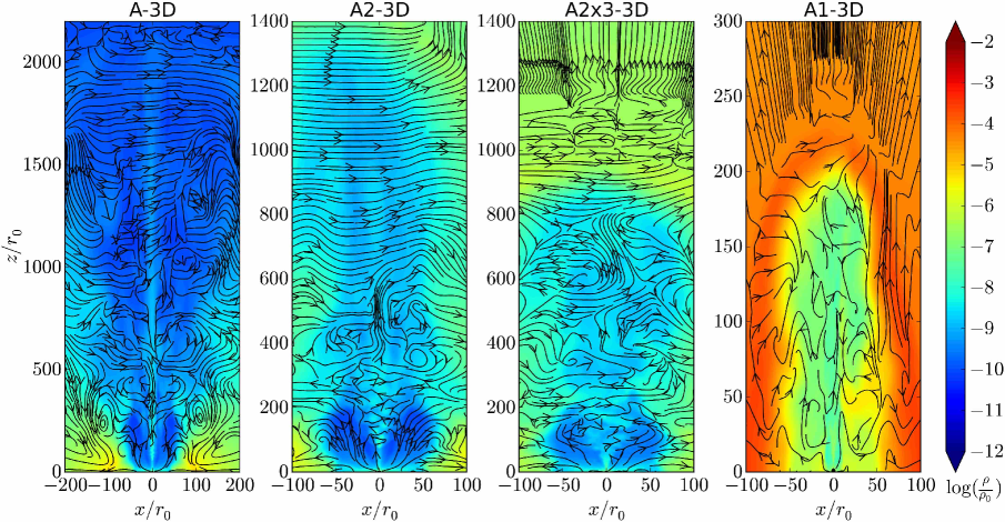
Figure 4: Side by side comparison of density snapshots in our 3D simulations at similar times (note the differences in length scales), with red showing high and blue low values (on a log scale; please see the colour bar). From left to right, we show vertical slices of density in models A ($t\approx 2700r_{0}/c$), A2 ($t\approx 3000r_{0}/c$), A2x3 ($t\approx 3400r_{0}/c$) and A1 ($t\approx 2800r_{0}/c$), respectively. Black directed lines show magnetic field streamlines traced out in the image plane. The perturbed nature of magnetic lines reflects both the emergence of irregular magnetic fields in the jets and the large-scale deviations of the jets out of the image plane, both caused by the 3D magnetic kink instability. Corresponding Lorentz factor contours of models A, A2, A2x3 and A1 can be found in Figs. 2, 3 and 6. The jet in model A2x3 propagates much slower than in A2, since it runs into the density higher by a factor of 3 at $r=100r_{0}$. Note that the jet in model A1 propagates $\sim 4$ times slower than in the model A2x3 due to an even higher density it encounters (this is because the break in the density profile in this model is at $r=10r_{0}$). The degree of deviation from axisymmetry increases from left to right. We conclude that an increase in ambient density leads to a stronger magnetic kink instability and, as we will see in the text, stronger magnetic energy dissipation.

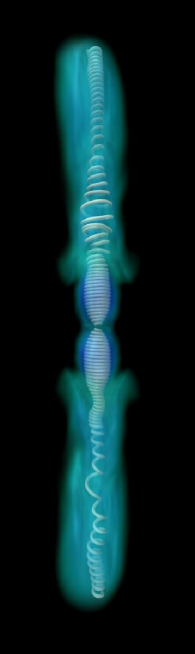
Figure 5: 3D rendering of density of our 3D simulation of model A2x3 at $t\approx 2200r_{0}/c$. The compact object is located at the center of the figure; this is the only figure that shows both jets. The jets extend to $z\sim 650r_{0}$. We have chosen a representative magnetic field line (white), which is twisted as the compact object rotates. The density breaks at $100r_{0}$ to a shallower density profile, which causes the jets to recollimate and the toroidal magnetic field to build-up and become unstable to the 3D magnetic kink instability. The irregular bends and asymmetries of the magnetic field lines are tell-tale signs of the instability. The instability dissipates toroidal magnetic field into heat around the density break and leads to a less tightly wound magnetic field at large radii.

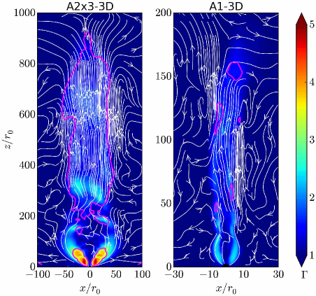
Figure 6: Cuts through the rotational axis of the Lorentz factor colour map of our 3D simulations A2x3-3D ($t\approx 3400r_{0}/c$) and A1-3D ($t\approx 2800r_{0}/c$) in the left and right panels, respectively. Both jets show deviations from axisymmetry due to the magnetic kink instability. The magenta lines show the position of the fast magnetosonic surface, while the white directed lines show the velocity streamlines traced out in the image plane. Note that these panels are zoomed-in versions of the density contours for these simulations shown in Fig. 4. The A2x3-3D jet turns sub-fast as it recollimates between $z\sim 100-200r_{0}$ close to the location of the density profile break, whereas the A1-3D jet remains always sub-fast (except for small super-fast patches) since the density break is placed very close to the central object, resulting in an insufficient dynamic range for the jet to accelerate to a super-fast velocity.

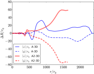
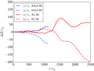
Figure 7: Non-axisymmetric modes in our headed jets, which drill into the ambient medium (A models, see Table 2), as measured through the deviation of jet “center of energy flux”, $\langle x\rangle$ and $\langle y\rangle$, from the rotational axis, $x=y=0$. These non-axisymmetric modes are only seen in 3D and signal the development of 3D instabilities. Top panel: The simulation A2-3D (dashed red lines), which has a density break at $100r_{0}$, shows larger deviations from axisymmetry than simulation A-3D (blue lines), which does not have a density break. The measurements are performed at the end of each simulation ($t\approx 3000r_{0}/c$ for A2-3D and $t\approx 2700r_{0}/c$ for A-3D). The jet remains axisymmetric until the recollimation point; however, beyond it, the jet shows deviations from axisymmetry. Bottom panel: Deviations from axisymmetry for the simulations A2x3-3D (blue lines) and A1-3D (dashed red lines) at the end of the simulations ($t\approx 3400r_{0}/c$ and $t\approx 2800r_{0}/c$, respectively). The presence of a jump in simulation A2x3 at $r_{t}=100r_{0}$ destabilizes the jet more than in simulation A2-3D, which is shown in the top panel and does not have the density jump. Simulation A1-3D also shows a large degree of asymmetry, as expected for jets of lower power (their power is 10x lower than for A2-3D and 3 times lower than for A2x3-3D). For ease of comparison across the models, we zoomed in on the simulation A1-3D by a factor of 10 times (i.e., just for this plot, we redefined $r_{0}=0.1r_{\rm in}$ instead of $r_{\rm in}$ so that the density break is now at $r_{t}=100r_{0}$ instead of $10r_{0}$).

Fig. 3 shows a sequence of snapshots of our 3D simulation of model A2, which we refer to as simulation A2-3D (see Table 3). We show colour maps of the slice through the rotational axis of the Lorentz factor. For this simulation, the recollimation point is much more noticeable and violent than in model A; it also propagates much more slowly. It settles at $z\sim 200r_{0}$, around the location of the external medium density break. Although it continues to move, the recollimation point moves only at $v\sim 0.1c$ towards the end of the simulation. Given that the external medium is not completely rigid, but it is allowed to be pushed by the jet, the recollimation point continuously moves out in our simulations. Similar to the A-3D jet, the magenta lines in Fig. 3 show that the A2-3D jet moves at a super-fast magnetosonic velocity beyond $z\sim 20r_{0}$. Also similar is that the jet accelerates to nearly $\Gamma\sim 10$ and once it passes through the recollimation point, it slows down. The presence of the break in the density profile at $r_{t}\sim 100r_{0}$ not only makes the jet recollimate more effectively, but also leads to a stronger deceleration of the jet, down to $\Gamma\sim 3$.

Beyond the recollimation point the jet develops substantial asymmetries, characteristic of 3D, non-axisymmetric magnetic kink instability. For simplicity of comparison, we show the simulations A-3D and A2-3D side by side in the two leftmost panels of Fig. 4. This makes it clear that the interaction of the jet with the break in the ambient density slows down the propagation of both the jet head and the recollimation point. The flattening of the density profile also causes the jet to become more collimated and change its shape from the parabolic-like well inside the recollimation point to cylindrical-like well outside of the break in density.

Because X-ray observations of density profile in M87 are consistent with a density jump accompanying the density break at the Bondi radius (Russell et al., 2015), we also consider model A2x3. In addition to the density break of model A2, it also features a jump in density by a factor of $\chi=3$ at the position of the break, $r_{t}=100r_{0}$ (please see equation 2, the left panel in Fig. 1, and Table 1). The third panel from the left in Fig. 4 shows that the density jump causes the recollimation to be more violent and significantly slows down the jet compared with the A2-3D run. Indeed, as Fig. 5 shows, whereas at small radii the jets maintain an ordered structure of a tightly wound axisymmetric helix, beyond the recollimation point the jet helix (i) develops significant asymmetries and irregularities characteristic of the 3D magnetic kink instability and (ii) becomes much less tightly wound. The two effects are related to each other: the 3D instability dissipates the magnetic energy by reducing the dominant toroidal magnetic field component and thereby also reducing the tightness of the helix (see also Bromberg & Tchekhovskoy 2016). The left panel of Fig. 6 shows that the A2x3-3D jet reaches a lower Lorentz factor $\Gamma\sim 5$ before the recollimation point and a lower $\Gamma\sim 2$ beyond it, as compared to model A2. More importantly, as opposed to a density break, the combination of the break and the jump causes the jet to slow down significantly and turn sub-fast magnetosonic. After the recollimation point, the jet accelerates and becomes super-fast again.

Note that in order for a jet to switch from super-fast to sub-fast speeds it needs to go through a shock. Dissipation, associated with such a shock, might in principle be observable. However, we found that in our simulations, such shocks dissipate a very small fraction of jet power, $\mathrel{\hbox{\hbox to0.0pt{\hbox{\lower 4.0pt\hbox{$\sim$}}\hss}\hbox{$<$}}}5$%, an order of magnitude less than the internal magnetic kink instability; see Sec. 3.2.

In order to investigate the sensitivity of our results to variations in jet power, we also carried out simulation A1-3D, which has the density break at a smaller distance ($r_{t}=10r_{0}$) without a jump ($\chi=1$), see Tables 1 and 3, and Fig. 1. The smaller distance to the density break results in a jet that propagates in a denser ambient medium. Effectively, this corresponds to a jet power that is $10$ times weaker than in model A2. Because weaker jets propagate at slower speeds, the smaller distance to the density break allows us to keep the simulation costs down for the same physical distance covered by the jet. It takes approximately $\sim 6$ times longer for the jet in model A1 to reach the same physical distance as in model A2.

The Lorentz factor of the A1-3D jet is presented in the right panel of Fig. 6, which shows a recollimation point at $\sim 25r_{0}$ and a much slower jet compared with the models discussed so far. It also shows that essentially the entire jet remains sub-fast (except for small super-fast patches). This is not surprising, because as we saw for the previous models the location of the fast surface is at $z\sim 20r_{0}$, which would fall beyond the break in density for model A1. This is why in all our previous models we placed the break in density profile at $z\sim 100r_{0}$, so that our jets accelerate to super-fast magnetosonic velocities by the time they reach the break in the ambient medium as we expect realistic AGN jets to do. Given that the A1-3D jet remains sub-fast, it describes a different astrophysical system, more akin to short- and long-duration GRB jets very close to their launching site than to AGN jets. We will investigate the differences between the stability and other properties of sub-fast and super-fast jets in future work.

The rightmost panel of Fig. 4 and the right panel of Fig. 6 show that the weaker A1-3D jet inflates a cavity with clear small-scale and large-scale asymmetries that reflect the development of small-scale, internal kink modes, which operate inside the jet, and global, external kink instability modes, which operate at the interface between the jet and the ambient medium. We have seen that these instabilities can be active at different levels in the headed jets presented so far. We now investigate these instabilities in more detail.

3.1.2 Deviations from axisymmetry and role of 3D instabilities

As seen in Figs. 2–6, the 3D models we have considered so far remain mostly axisymmetric at distances smaller than the recollimation point, at which the jets pinch toward the axis. However, beyond the pinch some deviations from axisymmetry are evident, both in density and Lorentz factor colour maps. While these deviations are small for model A, they increase substantially for other models featuring an obstacle in the jet’s way, e.g., in models A1 and A2 with a density break and even more so in the model A2x3 with a density break and jump.

We quantify the degree of jet non-axisymmetry by measuring the deviation of the jets from the rotation axis. To do this, we take the last snapshot of each of our simulations and compute the total energy flux $\dot{E}$ (without the rest-mass contribution) weighted values of the transverse coordinates, $x$ and $y$, as follows:

$$\langle x\rangle=\frac{\int\!x\,\mathrm{d}\dot{E}}{\int\!\,\mathrm{d}\dot{E}},$$ (3)

and similarly for the $y$ coordinate. In the case of an axisymmetric jet, we expect the total energy to be symmetric along the $-x$ and $+x$ (and also along the $-y$ and $+y$) directions, yielding $\langle x\rangle=0$ ($\langle y\rangle$=0). Thus, the deviations of $\langle x\rangle$ and $\langle y\rangle$ from zero offer us a quantitative measure of jet deviations from axisymmetry.

We calculate $\langle x\rangle$ and $\langle y\rangle$ for our model A jet and plot these as a function of the radial coordinate $r$ in the top panel of Fig. 7. We see that the jet remains mostly axisymmetric, with very small deviations from the axial symmetry, before it passes through the recollimation point. Even after the jet passes through it, its deviations from axisymmetry remain quite small relative to the width of the jet, as seen in Figs. 2 and 4.

In the top panel of Fig. 7, we also show the same diagnostics for model A2 whose only difference from model A is the presence of a density break at $r_{t}=100r_{0}$. The presence of the break causes the deviations from axisymmetry to rapidly increase beyond the recollimation point and most of the jet energy flux to shift away from the rotational axis. In fact, the tip of the jet is displaced a distance from the rotational axis comparable to the width of the jet. These deviations from axisymmetry can be quite easily seen for both the density and Lorentz factor colour maps of model A2 in Figs. 3 and 4. This shows that even smooth changes in the external medium can have a qualitative effect on the structure of the jets.

We also compute the same diagnostics for the jets in models A2x3 and A1 and show them in the bottom panel of Fig. 7. Noticeable deviations from axisymmetry are found also for these models, with the strongest deviation in the lowest-power model, A1. This is consistent with the findings of Bromberg & Tchekhovskoy (2016) who find that the lower the power of a jet, the less stable it is to the external kink instability.

3.1.3 Comparison to 2D simulations

In order to understand the role of 3D instabilities on the jet structure and emission, we compare the 3D simulation results described above to 2D simulations results. Because 3D instabilities are not present in 2D simulations, the differences between 2D and 3D simulations tell us about the effect of non-axisymmetric instabilities on the structure of the jets, including internal dissipation. Furthermore, because we can carry out convergence tests in 2D with rather little computational expense, comparison to 2D simulations at different resolutions allows us to quantify the effect of the resolution changes on our results. This, of course, does not replace the proper 3D convergence studies, which we also perform, as we discuss below. We present most of our 2D simulations and 2D convergence tests in Appendix A, but discuss the main features of the 2D simulations results in the main text.

We have performed 2D simulations of our headed jets at different resolutions, see Tables 2 and 3. All our 3D models that interact with a change in the external medium (e.g., all A models except A-3D) show much slower propagation of the jet head compared with 2D models. Also, as shown in Section 3.1.2, these 3D jets show deviations from axisymmetry, whereas 2D jets are axisymmetric by design. These non-axisymmetric modes cause the jets to slow down relative to 2D (Bromberg & Tchekhovskoy, 2016; Tchekhovskoy & Bromberg, 2016). The 3D instabilities also cause additional dissipation in the jets; we will now compare to 2D simulations to quantify this intrinsically 3D effect.

3.1.4 Energy dissipation

A major goal of this study is to understand whether and how changes in the external medium affect jet structure and cause internal energy dissipation. For this, we plot the contributions of different energy flux components to the total energy flux, $\dot{E}$, as a function of radius: (i) the electromagnetic energy flux, $\dot{E}_{\rm EM}=\iint 2p_{\rm mag}\Gamma^{2}v_{r}\,{\rm d}A$, (ii) the kinetic energy flux, $\dot{E}_{\rm KE}=\iint\rho\Gamma(\Gamma-1)v_{r}\,{\rm d}A$, and (iii) the enthalpy flux, $\dot{E}_{\rm INT}=\iint(u_{g}+p_{g})\Gamma^{2}v_{r}\,{\rm d}A$, where $\rho$, $u_{g}$, $p_{g}\equiv(\gamma-1)u_{g}=u_{g}/3$, and $p_{\rm mag}$ are density, internal energy, thermal pressure, and magnetic pressure, all measured in the fluid frame; $\Gamma$ is the Lorentz factor and $v_{r}$ is radial velocity. The integration is carried out over a sphere, and ${\rm d}A=r^{2}\sin\theta\,{\rm d}\theta\,{\rm d}\varphi$ is the area element. At the base of the jet essentially all of the energy flux is in the electromagnetic form. It transforms to kinetic energy as the jet accelerates and to internal energy as the jet dissipates. The distance at which the energy flux drops to zero marks the location of the jet head.

We calculate these energy fluxes at the final time of our simulations, when the head of the jet has reached a distance at least a factor of $\sim 10$ times larger distance than where the change of the external medium occurs. In order to isolate the role of 3D instabilities in the energy dissipation in the jets, we will compare the energy fluxes in 3D and 2D simulations at the same spatial resolution, $N_{r}\times N_{\theta}$.

We first focus on model A and show its energy flux components in the left panel of Fig. 8. In the A-2D simulation, the electromagnetic energy decreases at $r\mathrel{\hbox{\hbox to0.0pt{\hbox{\lower 4.0pt\hbox{$\sim$}}\hss}\hbox{$>$}}}100r_{0}$, whereas the internal energy increases. However, at higher resolutions in 2D, the internal energy increase becomes suppressed. This indicates that the most likely origin of this increase is numerical dissipation due to insufficient resolution (see Appendix A). We draw the same conclusion regarding simulation A-3D, since its energy content is quite similar to the A-2D simulation. In addition, given that the A-3D jet is approximately azimuthally symmetric (see top panel of Fig. 7), 3D instabilities, which could dissipate the electromagnetic energy and make the jet wobble, are either not present or quite weak for this model.

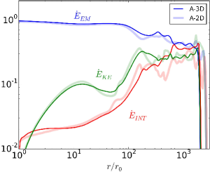
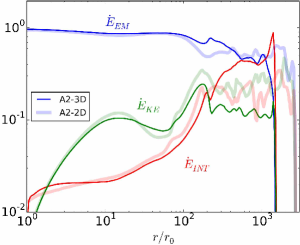
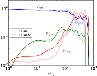
Figure 8: Different components of the energy flux (see labels) for 3D and 2D simulations (see legends) of models A ($t\approx 2700r_{0}/c$) and A2 ($t\approx 3000r_{0}/c$) in the left and middle panel, respectively. The energy fluxes have been normalized to the value of the total energy flux at $r=r_{0}$. The distance at which the energy flux drops to zero marks the location of the jet head. In the right panel we present the results of our A2-3D-hr simulation compared to those of A2-3D (at $t\approx 1500r_{0}/c$). Model A shows a similar level of electromagnetic energy dissipation in 3D and in 2D (left panel). However, model A2 shows a large increase in internal energy compared to what it is seen in 2D, due to the presence of 3D instabilities (middle panel, for $\mathrel{\hbox{\hbox to0.0pt{\hbox{\lower 4.0pt\hbox{$\sim$}}\hss}\hbox{$>$}}}300r_{0}$). The A2-3D-hr run shows even more electromagnetic energy dissipation and higher internal energy than the A-3D run implying that high resolution is required to follow the development of the MHD instabilities (right panel).

The middle panel of Fig. 8 shows various contributions to the total energy flux in the simulation A2. Whereas the level of dissipation in 2D is similar to the model A without a break, in our 3D simulation A2-3D, the jet internal energy exceeds that in 2D simulation by a factor of 2 beyond the break, $r\mathrel{\hbox{\hbox to0.0pt{\hbox{\lower 4.0pt\hbox{$\sim$}}\hss}\hbox{$>$}}}100r_{0}\sim r_{t}$. Additionally, the 3D jet shows clear deviations from axisymmetry, as seen in the top panel of Fig. 7. This suggests that 3D instabilities are at work in this jet. In order to verify this, we have repeated the simulation A2-3D at twice as high resolution in each direction. We refer to this run as the simulation A2-3D-hr (see Table 2). The right panel in Fig. 8 shows that the higher-resolution simulation A2-3D-hr exhibits a stronger decrease of electromagnetic energy flux at $r\mathrel{\hbox{\hbox to0.0pt{\hbox{\lower 4.0pt\hbox{$\sim$}}\hss}\hbox{$>$}}}100r_{0}\sim r_{t}$ accompanied by a more prominent increase of internal energy flux than in the A2-3D simulation. Fig. 9 compares vertical slices through density distributions in the two simulations. The A2-3D-hr jet propagates $30$% slower than the A2-3D one, due to the better resolution of the external kink instability that slows down the jet propagation (Bromberg & Tchekhovskoy, 2016).

To summarize, the higher resolution 3D simulation A2-3D-hr shows more energy dissipation than our fiducial resolution simulation A2-3D. This confirms the robustness of 3D instabilities in our headed jets and their role in dissipating the internal energy. In fact, the high-resolution jet dissipates as much as $70$% of its energy flux into heat, more than sufficient to account for the observed emission in jets. Higher resolution also resolves better the global 3D instabilities and motions of the jet head. These instabilities substantially slow the jet down as the jet head wobbles. We conclude that the presence of a break in the density profile favors the development of 3D instabilities and considerably strengthens the dissipation in headed jets.

So far we have considered models with jets propagating into continuous ambient density profiles. The top panel of Fig. 10 illustrates jet energy dissipation in model A2x3, in which a jet navigates a jump in the external density by a factor of 3 in addition to the density break. Whereas the 2D version of this model, A2x3-2D, shows a similar level of dissipation to the simulation A2-2D (which does not have a jump), in the 3D version, A2x3-3D, the presence of the jump increases the fraction of electromagnetic energy converted into heat substantially: as much as $80$% of jet electromagnetic energy is converted into heat in the A2x3-3D jet, which is much higher than the $20$% level of dissipation seen in the 2D models A2x3-2D and A2-2D (this level of dissipation in 2D models is due to limited numerical resolution, as we show in Appendix A). The high fraction of dissipated energy, coupled with the deviations from axisymmetry seen for this model (see the bottom panel of Fig. 7), makes a strong case for the presence of 3D instabilities and their role in causing the dissipation of electromagnetic into thermal energy in the headed jets that run into an obstacle in the ambient medium. Additionally, the presence of a density jump in the ambient medium is favorable for the growth of instabilities and energy dissipation.

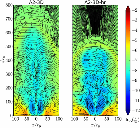
Figure 9: 2D cut of density contours of the A2-3D simulation (left panel) and the A2-3D-hr one (right panel) at the final run time of the latter ($t\approx 1500r_{0}/c$). Black arrows show magnetic field streamlines. The higher resolution A2-3D-hr simulation propagates much slower and inflates a bigger cavity, since it is able to better resolve the kink instability that slows down the jet propagation as the jet head wobbles.

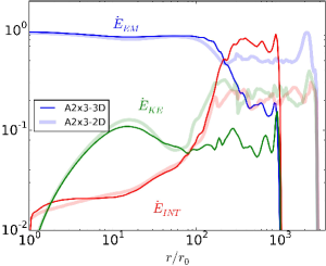
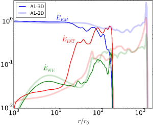
Figure 10: Different components of the energy flux (see labels) for 3D and 3D simulations (see legends) of models A2x3 ($t\approx 3400r_{0}/c$) and (A1 at $t\approx 2800r_{0}/c$) in the top and bottom panel, respectively. Both models show a decrease in electromagnetic energy flux accompanied by an increase in internal energy flux in 3D at the location of the density break. The energy dissipation is much more prominent than what is seen in 2D.

The bottom panel of Fig. 10 illustrates the energy dissipation in model A1. This model corresponds to a lower power jet propagating into a density profile with a break (without a jump) at $r_{t}=10r_{0}$. For this model, the A1-2D simulation shows an approximately constant value of the electromagnetic energy flux as a function of radius. However, the A1-3D run shows a decrease in the electromagnetic energy flux, which occurs right at the location of the density break $r_{t}\sim 10r_{0}$, and is accompanied by an increase in the internal energy flux at the same location. At large radii, the internal energy flux is at least 50% of the total jet power. These features are not seen at any resolution in the 2D simulations (see Appendix A). Thus, the dissipation and the high degree of asymmetry in the shape of the A1-3D jet (see bottom panel of Fig. 7) strongly indicate the presence of 3D instabilities and their contribution to the internal jet dissipation.

3.2 Sub-fast and super-fast regions and dissipation

As we discussed in Sec. 3.1.1, 3D jets in models A and A2 are super-fast magnetosonic. However, Figs. 2 and 3 show that a fraction of the jet around the polar axis remains sub-fast. This sub-fast region “knows” about the impending collision with the ambient medium and develops an internal 3D kink instability that converts magnetic into thermal energy. Since energy flux in jets is edge-concentrated (Tchekhovskoy, McKinney & Narayan, 2008), these polar sub-fast regions contribute very little to the internal energy flux, only about a few per cent of the total jet power. The jet in model A2x3 develops larger sub-fast regions (see Fig. 6) with an internal energy flux that makes up $\sim 15$% of the total jet energy flux; the super-fast regions carry $\sim 65$% of the total energy flux, which together yield the $\sim 80$% total internal energy flux seen at large radii in Section 3.1.4 for this simulation. For the 3D jet in model A1, which remains sub-fast throughout except for small super-fast patches, the internal energy flux in the sub-fast regions is at the $\sim 10$ % level of the total jet energy flux.

In regions where the jets go from being super-fast to sub-fast magnetosonic (e.g., in model A2x3-3D, left-panel of Fig. 6), a shock forms and slows down the flow. More generally, we expect such a shock to form every time a super-fast flow rams into the ambient medium. We expect the shock to dissipate some energy; however, given the high magnetization at the location of the shock, we expect the dissipation to be rather weak (e.g., Mimica, Giannios & Aloy, 2010). There is evidence for the presence of such shocks, for example, in the energy fluxes of the high-resolution 2D simulations of model A2x3, where a sharp increase in internal energy flux is observed at $r\sim 150r_{0}$ (see Appendix A). However, as expected, the internal energy flux at the post-shock region is small, $\mathrel{\hbox{\hbox to0.0pt{\hbox{\lower 4.0pt\hbox{$\sim$}}\hss}\hbox{$<$}}}5$%. Even though energy dissipation at the shock is small, by slowing down the flow the shock triggers the development of MHD instabilities downstream that can efficiently dissipate magnetic energy.

The presence of a shock can also be identified by the variation of entropy,

$$s=\frac{1}{\gamma-1}\ln\left(\frac{p_{g}}{\rho^{\gamma}}\right),$$ (4)

where $p_{g}=(\gamma-1)u_{g}=u_{g}/3$ is the thermal pressure. This diagnostic is an alternative to the inspection of energy fluxes discussed above (which are angle-integrated quantities and thus are not well-suited for identifying dissipative features that are extended in radius, such as conical shocks). We show a colour map of entropy in a vertical slice through the jet axis of model A2-3D-hr in the left panel of Fig. 11. The low-entropy flow (since the jet is initially cold) is super-fast at the end of the simulation and turns sub-fast around $z\sim 80r_{0}$. Interestingly, just as the flow turns sub-fast, the entropy increases abruptly (the fast magnetosonic surface and the entropy increase match precisely), indicating the presence of a shock as discussed above. This entropy plot very clearly highlights the various dissipation regions in our headed jets discussed above: the dissipative cone at small radii along the jet axis and the internal kink at larger radii. Both of these are regions that can also be identified in, e.g., Fig. 3.

As mentioned in Bromberg & Tchekhovskoy (2016), the magnetic kink instability is triggered as the flow passes through the recollimation region. They derived an instability criterion that they applied to their particular scenario of mildly relativistic, $\Gamma\approx 1$, and initially weakly collimated jet that runs into an ambient medium. Our jets move relativistically and are highly collimated. The stability criterion that describes our jets remains to be studied in detail. However, in analogy with the work of Bromberg & Tchekhovskoy (2016), the growth time-scale of the magnetic kink instability is proportional to the magnetic pitch, which is the ratio of the poloidal to toroidal magnetic field strength in the comoving frame, $b_{\rm p}/b_{\phi}$ (see, Appl, Lery & Baty, 2000, e.g.,). We show a colour map of $\log_{10}(b_{\rm p}/b_{\phi})$ for the A2-3D-hr jet in the right panel of Fig. 11, which can be easily compared to the entropy colour map in the left panel. The narrow jet, which extends from $x\sim-50r_{0}$ to $x\sim 50r_{0}$ shows $b_{\rm p}/b_{\phi}<1$ at small radii, which suggests a rapid growth of the magnetic kink instability. At larger radii, the region with $b_{\rm p}/b_{\phi}>1$ grows in size, suggesting that the jet turns stable at large radii (see Bromberg & Tchekhovskoy, 2016). This happens because the toroidal component of the magnetic field, $b_{\phi}$, which dominates at small radii and turns the jet kink unstable, is dissipated away as the magnetic energy is converted to internal energy. After this occurs, $b_{\phi}$ decreases making the jet less susceptible to the kink instability. This can be also clearly seen in Fig. 5, where the irregular bends and asymmetries of the magnetic field lines become dissipated away. This causes the field to become less tightly wounded and more ordered at large radii.

Summing up, the presence of obstacles in the ambient density, such as a factor of few jump in density, or even just a break in the density slope, can have a dramatic effect on jets in 3D. These features can lead to the development of 3D instabilities and prominent dissipation, up to $\mathrel{\hbox{\hbox to0.0pt{\hbox{\lower 4.0pt\hbox{$\sim$}}\hss}\hbox{$>$}}}50$% of the total jet flux (see Figs. 8 and 10). This dissipation might power bright features in jets and the blazar zone as we discuss in Secs. 4 and 5.

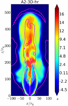
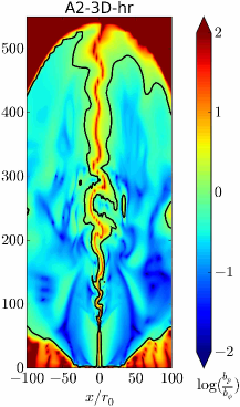
Figure 11: Left panel: Vertical slice through entropy in the A2-3D-hr simulation at the final run time, $t\approx 1500r_{0}/c$. The magenta lines show the position of the fast magnetosonic surface. At $z\mathrel{\hbox{\hbox to0.0pt{\hbox{\lower 4.0pt\hbox{$\sim$}}\hss}\hbox{$>$}}}10r_{0}$, the jet crosses the fast magnetosonic surface the first time and turns from sub- to super-fast magnetosonic. At $z\mathrel{\hbox{\hbox to0.0pt{\hbox{\lower 4.0pt\hbox{$\sim$}}\hss}\hbox{$>$}}}50r_{0}$ the jet crosses the fast surface the second time, this time turning from super- to sub-fast magnetosonic. This second fast surface is a fast shock at which the entropy sharply increases. The entropy increases further beyond the shock, at $z\mathrel{\hbox{\hbox to0.0pt{\hbox{\lower 4.0pt\hbox{$\sim$}}\hss}\hbox{$>$}}}100r_{0}$, due to the internal kink instability. Right panel: 2D cut of $\log_{10}(b_{\rm p}/b_{\phi})$ contours of the A2-3D-hr simulation at the final run time ($t\approx 1500r_{0}/c$). The black lines show the surface where $b_{\rm p}/b_{\phi}=1$ roughly dividing the regions where the jet is more ($b_{\rm p}/b_{\phi}<1$) and less ($b_{\rm p}/b_{\phi}>1$) susceptible to the magnetic kink instability. As the magnetic energy is dissipated by the kink instability and converted to internal energy, the jet turns more stable to this instability.

3.3 Headless jet interacts with the external medium

3.3.1 Modeling the external medium

In Sec. 1, we discussed the distinction between jets of two types different by whether they drill through the ambient medium: headed and headless jets. In Sec. 3.1, we considered how headed jets, which drill through the ambient gas, are affected by the changes in the external medium density profile. Here, we perform a similar analysis for headless jets, which do not have to drill through the ambient medium because, e.g., they have a pre-existing funnel to propagate through. We expect such jets in several astrophysical scenarios (see Sec. 1). In the AGN context, we would like to model a jet that propagates outward through essentially an empty (or very low-density) funnel and collimates against the surrounding accretion disc outflow. In this case, we can think of the walls of the funnel as providing the confining medium for the jet and setting the jet shape.

In order to model such jets, we use a density distribution of the form

$$\rho_{\rm B}=\rho_{0}\left(\displaystyle\frac{r}{r_{0}}\right)^{-\alpha}\sin^{\delta}\theta,\qquad\text{(Model B)}$$ (5)

where $\theta$ is the polar angle (the angle measured with respect to the jet axis). As in model A, we adopt $\alpha=3$ and, similarly, choose $\rho_{0}=4500$ and $B_{0}=(4\pi)^{1/2}$, the initial density and magnetic field strength at $r_{0}$, respectively. The $\sin^{\delta}\theta$ term effectively evacuates the density along the rotational axis and essentially prescribes the shape of the walls of the funnel. We will refer to this as model B, see Table 1 and the middle panel in Fig. 1. This density mimics what is seen in simulations of thick accretion discs (e.g., De Villiers et al., 2005; McKinney, 2006; Tchekhovskoy, Narayan & McKinney, 2011); a more detailed comparison will be left for a future study.

We refer to our 3D simulation of model B as simulation B-3D (see Table 3 for more details). In the left panel of Fig. 12, we show the colour map of density in a vertical slice through the jet axis. We see that the jet propagates along the funnel as it expands sideways, maintaining roughly a parabolic shape. At large radii, the jet attains a Lorentz factor of $\sim 7$.

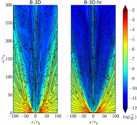
Figure 12: 2D cut of density contours of the B-3D simulation (left panel) and the B-3D-hr one (right panel) at the final run time of the latter ($t\approx 1200r_{0}/c$). Black arrows show magnetic field streamlines. The jet propagates along the funnel as it expands sideways. The B-3D and B-3D-hr simulations are quite similar. We have zoomed-in on a region $z<300r_{0}$ even though the jet head is at $\sim 1200r_{0}$. There are no significant deviations from axisymmetry in this model.

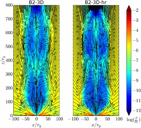
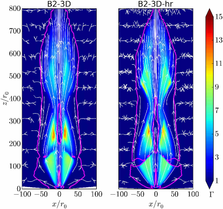
Figure 13: 2D cut of density contours (top panels) and Lorentz factor contours (bottom panels) of the B2-3D simulation (left panels) and the B2-3D-hr one (right panels) at the final run time of the latter ($t\approx 700r_{0}/c$). Black arrows in the top panels show magnetic field streamlines. White arrows in the bottom panels show velocity streamlines and magenta lines show the location of the fast-magnetosonic surface (most of the jet, colored regions, is super-fast, except for a small thin region along the jet-axis; this will be discussed in Section 3.3.4). The jet is confined to propagate in a pre-existing funnel that becomes cylindrical at $z=80r_{0}$. The presence of conical shocks is evident by inspecting the Lorentz factor plots (as coloured shapes with a sharp boundary). We see a conical shock at $z\sim 150r_{0}$ and another one between $z\sim 200-300r_{0}$. The B2-3D-hr simulation shows a more defined structure between $z\sim 400r_{0}$ and $600r_{0}$ and the presence of yet another conical shock in this region.

Now that we have simulated a jet confined by an accretion disc, we would like to modify the set up so that the jet eventually interacts with the ambient medium. We model this interaction by adjusting the shape of the funnel to abruptly become cylindrical. Because the funnel is essentially empty, the jet does not have to drill through the ambient medium and remains headless. Namely, we consider the following density distribution

$$\rho=\begin{cases}\rho_{\rm*}(z)&|z|\leq z_{0}\\ \rho_{\rm*}(z_{0})&|z|>z_{0},\end{cases}\qquad\text{(Model B\#)}$$ (6)

where $z=r\cos\theta$ is the distance along the jet axis of rotation, and $z_{0}$ is the distance beyond which we “freeze” the lateral profile of the external medium at the value of $z=z_{0}$, that is, the funnel becomes cylindrical. In order to ensure that the funnel walls are heavy enough to prevent the jet from displacing them, we use

$$\rho_{\rm*}=\begin{cases}\rho_{\rm B}(r)&r\leq r_{t}\\ \chi\left(\displaystyle\frac{r}{r_{t}}\right)^{-\beta}\rho_{\rm B}(r=r_{t},\theta=\pi/2)&r>r_{t},\end{cases}$$ (7)

with $\beta=1$, $r_{t}=100r_{0}$ and $\chi=3$. In equation (6) we choose $z_{0}=80r_{0}$, which leads to a cylindrical funnel of radius $\simeq 60r_{0}$. We refer to this setup as model B2, see Tables 1 and 3 and the right panel in Fig. 1.

We show a snapshot of our 3D simulation, B2-3D, in Fig. 13 (left panels), where we present the slices through the density and Lorentz factor contour maps. The cylindrical funnel confines the jets and forces them into a cylinder. We find that, at the location where the funnel transitions to being cylindrical, the jet undergoes a conical shock as evident by the sharp feature in the Lorentz factor seen in the bottom-left panel of Fig. 13, especially the features at $(x,z)\sim(\pm 40r_{0},150r_{0})$. There is also a second conical shock, between $z\sim 200-300r_{0}$, whose surface is close to the jet axis. We discuss these conical shocks below.

Our jets in models B and B2 propagate close to the speed of light, because they propagate along an evacuated funnel and do not have to do work against the external medium. This is also why they easily accelerate to super-fast magnetosonic velocities before they encounter changes in the ambient medium, just like jets in nature. Indeed, the bottom left panel of Fig. 13 shows that the jets cross the fast surface at around $z\sim 10r_{0}\ll z_{0}$. This is important, as we discussed previously, because if this were not the case, the ambient medium would be able – in an unphysical way – to affect the conditions of the jets near the central compact object.

3.3.2 Deviation from axisymmetry and role of 3D instabilities

We have calculated the deviations from axisymmetry for models B-3D and B2-3D by calculating $\langle x\rangle$ and $\langle y\rangle$ as described in Section 3.1.2. Only extremely small deviations of the order of $\langle x\rangle/r_{0}\sim\langle y\rangle/r_{0}\sim 1$ are observed for these simulations at the final times of the runs. For models B-3D and B2-3D, this result shows that headless jets tend to maintain their axisymmetry, even when they navigate abrupt changes in the jet shape. Indeed, even after passing through recollimation shocks, the jets do not develop global 3D instabilities, although this is perhaps not so surprising given that the shape of the jet is held fixed by the hard wall. This is in agreement with Bromberg & Tchekhovskoy (2016), who found that headless jets are more stable than their headed counterparts. The absence of global 3D stabilities of headless jets enables us to use 2D simulations for studying most of the large-scale dynamics of these jets.

3.3.3 Numerical convergence of jet morphology

To ensure that our simulations are numerically-converged, we perform 2D and 3D simulations of models B and B2 at various resolutions (see Tables 2 and 3). For model B, 3D simulations at various resolutions are quite similar: both maintain roughly a parabolic shape, as seen in Fig. 12. The jets propagate at a very similar velocity. The jet of model B-3D-hr is a bit wider due to the increase of $N_{\theta}$-resolution and the ability to resolve better the interface between the jet and the pre-carved funnel. Our 2D simulations reproduce the main features seen in 3D simulations reflecting the near absence of 3D instabilities in headless jets (see Appendix B).

Likewise, Fig. 13 shows that the simulations of model B2 at different resolutions show very similar jet shapes and jet propagation velocities. The jets show conical shocks, seen as sharp jumps in density and Lorentz factor. In Appendix B, we show that these features are present in both 2D and 3D simulations of model B2 and therefore are not inherent to 3D. Because the shocks are oblique, most of the jet flow remains super-fast magnetosonic even after passing through the shocks. The first set of shocks at $z\sim 100r_{0}$ occurs as the jet accelerates to the point that it drops out of lateral causal contact, i.e., its side-ways expansion becomes super-fast magnetosonic. The shock slows down the jet and brings it back into lateral causal contact with the ambient medium. The jet then collimates off the ambient medium, converges and accelerates into the jet axis. Note that this acceleration occurs due to jet sideways contraction, which is the opposite of the standard jet acceleration due to sideways expansion (Beskin & Nokhrina, 2006; Komissarov et al., 2007; Tchekhovskoy, McKinney & Narayan, 2008, 2009), and we discuss a possible reason for this unexpected behaviour in Sec. 4.

Once the motion toward the axis becomes super-fast magnetosonic, a second set of conical shocks develops, as seen at $z\sim 250r_{0}$, and slows down the transverse motion to sub-fast magnetosonic speeds. In fact, a small central part of the jet (closest to the axis) slows down so much that its net velocity becomes sub-fast magnetosonic. This region, marked by the magenta line, shows signs of 3D magnetic instabilities, as suggested by the irregular streamline shape seen at $x\simeq 0$, $z\simeq 300r_{0}$ in the bottom-right panel of Fig. 13. As we discuss in Sec. 3.3.5, these 3D instabilities dissipate a very small fraction of jet magnetic energy into heat.

After the second set of shocks, the jet bounces back and accelerates, and the shock structure repeats itself. In fact, at a higher resolution, a third set of conical shocks emerges around $z\sim 500r_{0}$ for the B2-3D-hr jet, as seen in the bottom right panel of Fig. 13. Even higher resolutions and longer run times, which we are able to achieve in 2D, point to the emergence of a regular, periodic shock structure formed by the bouncing jet that cannot come to terms with being confined by the cylindrical funnel, see Fig. 14.

The result is a wavy jet shape, with a pronounced “sausage” or “breathing” ($m=0$) mode. Related jet oscillations have been observed in the context of magnetized jets confined by a single power-law flat pressure profile medium analytically (Lyubarsky, 2009) and numerically (Mizuno et al., 2015; Komissarov, Porth & Lyutikov, 2015). We compare and contrast these results to ours in Sec. 4.

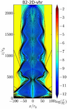
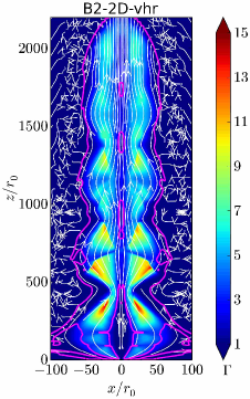
Figure 14: Density contour (left panel) and Lorentz factor contour (right panel) of the B2-2D-vhr simulation at the final snapshot, $t\approx 2200r_{0}/c$; note that the vertical scale is compressed relative to the horizontal. Black lines in the left panel show poloidal magnetic field streamlines. White arrows in the right panel show velocity streamlines and magenta lines show the location of the fast-magnetosonic surface. A series of conical shocks is seen throughout the cylindrical funnel, although the ones farther away from the central object are less well-resolved.

3.3.4 Energy dissipation

In this section, we analyze our headless jets in terms of their energy flux content (for a similar analysis of headed jets, see Section 3.1.4 and Figs. 8 and 10). To isolate the role of 3D effects, we compare the simulations B-3D and B-2D, in the top-left panel of Fig. 15. In both 2D and 3D, we see similar behaviour of the different energy flux components. There is a steady increase in the kinetic energy at the expense of the electromagnetic energy. This is expected, as the headless jets accelerate easier than the headed ones, and reach higher velocities. The internal energy shows a stronger increase starting at $r\sim 100r_{0}$. However, as the top-right panel of Fig. 15 shows, at higher resolution in 3D, this internal energy increase becomes substantially suppressed (see also Appendix A for a detailed 2D study). This indicates that this increase is mostly due to low numerical resolution, which shows up as dissipation at large distances. There are no 3D instabilities evident in this model, and the jet shape shows azimuthal symmetry: neither the jet head nor the body wobbles or is perturbed. This is consistent with our analysis of global instabilities in Sec. 3.3.2.

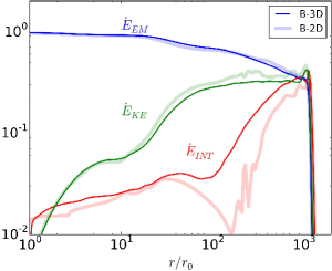
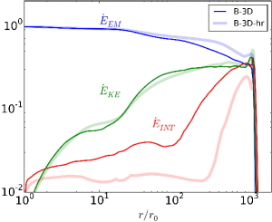
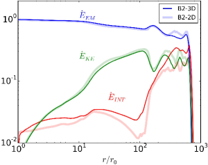
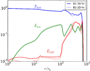
Figure 15: Different components of the energy flux (see labels) for 3D and 2D simulations (see legends) of model B ($t\approx 1200r_{0}/c$) and B2 ($t\approx 700r_{0}/c$) in the top and bottom panels, respectively. The top-left panel shows that model B exhibits similar levels of electromagnetic energy dissipation both in 2D and 3D, with an increase in internal energy close to $r\sim 100r_{0}$. However, the top-right panel shows that this increase goes away at higher 3D resolution, indicating that the jets in model B show no dissipation (see also the main text and Appendix A), but only a decrease of electromagnetic energy in order to accelerate the jet (not to heat it up). Model B2 exhibits oscillations in the kinetic energy due to the presence of multiple conical shocks, which slow down the jet, decrease the kinetic energy and convert it into electromagnetic and internal energy: see, e.g., the increase of $\dot{E}_{\rm EM}$ and $\dot{E}_{\rm INT}$ at $\sim 150r_{0}$ (bottom-left panel). The bottom-right panel shows the jet energy content for higher resolution runs. By comparing the bottom-left and bottom-right panels, we find that simulations B2-3D and B2-3D-hr show quite similar features in their energy content, indicating that they are numerically converged. Also the energy contents of the jets in B2-3D-hr and B2-2D-hr simulations (shown in the bottom right panel and carried out at the same $N_{r}\times N_{\theta}$ resolution) are almost identical, indicating that the contribution of 3D instabilities to dissipation in these jets is subdominant.

The change in the shape of the jet-confining wall into a cylinder in model B2 leads to qualitatively different jet behaviour, as seen in bottom-left panel of Fig. 15. Initially, the electromagnetic energy is converted to kinetic energy as the jet accelerates, just as we saw in model B. However, the situation changes at the break in the funnel shape. The bottom panels of Fig. 15 show that at different resolutions both our 2D and 3D simulations display a similar increase in the internal energy at the position of the break, $r\mathrel{\hbox{\hbox to0.0pt{\hbox{\lower 4.0pt\hbox{$\sim$}}\hss}\hbox{$>$}}}100r_{0}$. This conversion to internal energy occurs at the conical shocks, which are seen as jumps in the density and Lorentz factor in Fig. 13 (see also Sec. 3.3.3). The shocks slow down and heat up the jet, and compress the magnetic field. The bottom-left panel of Fig. 15 shows that in simulation B2-2D the kinetic energy decreases at the first shock at $r\sim 100r_{0}$ (a “dip” in the curve), while the electromagnetic energy increases (a “bump”) and the internal energy quickly rises. An oscillating pattern of the kinetic energy flux as a function of distance from the central object, as the jet encounters the second and third shock (less well-resolved), is also evident in the bottom panels of Fig. 15. The B2-3D jet shows the same features, while exhibiting azimuthal symmetry (Sec. 3.3.2). This robustly points to energy dissipation via conical shocks, which slow down the jets by converting the kinetic energy into heat and compression of the magnetic field. This is in contrast to headed jets, where the dissipation occurs due to 3D instabilities, as evident by not only the increase in internal energy, but also by the wobbling/asymmetric nature of the jets and the emergence of the irregular magnetic field structure and the current sheets.

To quantify the energy dissipation in headless jets, we consider the variation of entropy. In steady state, absent dissipation, entropy remains constant; it increases in the presence of dissipation. Fig. 16 shows the radial profiles of entropy and Lorentz factor along a representative streamline in our model B2-3D-hr. The streamline is shown in the figure inset. At small radii, the jet is cold and strongly magnetized. The application of density and internal energy “floors” in this region leads to deviations from constancy in the entropy profile. By $r\mathrel{\hbox{\hbox to0.0pt{\hbox{\lower 4.0pt\hbox{$\sim$}}\hss}\hbox{$>$}}}20r_{0}$, the magnetization drops due to the bulk flow acceleration by the magnetic fields, the density and internal energy floors are no activated, and the entropy profile settles to a constant, $s\approx-3.5$ that corresponds to essentially a cold jet. At the location of the shock, $r\sim 100r_{0}$, the entropy rises sharply and the Lorentz factor drops. Beyond the shock, the jet re-accelerates and the Lorentz factor smoothly increases.

The jet sharply decelerates at $r\sim 200r_{0}$ as it passes through the second conical shock. The entropy additionally increases at this shock, reflecting the shock heating experienced by the jet. By $r\sim 250r_{0}$, the Lorentz factor decreases to essentially non-relativistic values, $\Gamma\mathrel{\hbox{\hbox to0.0pt{\hbox{\lower 4.0pt\hbox{$\sim$}}\hss}\hbox{$<$}}}1.5$. This occurs when the streamline enters a sub-fast magnetosonic region, indicated by the magenta line, as seen on the figure inset. The flow in this small region is unstable to the internal 3D magnetic kink instability, which dissipates magnetic energy into heat. This dissipation is evidenced by the increase in the entropy of the streamline. Once the streamline exits the dissipative region at $r\sim 350r_{0}$, the entropy slightly decreases. While we would not expect such a decrease along a streamline in the steady state, we suggest that the time-dependent dissipation and irregular flow in the sub-fast region could cause this behaviour.

3.3.5 3D instabilities and heating in headless jets

Another way to study jet dissipation is through a map of entropy in the jets, shown in Fig. 17 for our high-resolution simulations of model B2. Because the jets start out cold, the entropy near the origin is low both in the left panel, showing the 3D simulation, B2-3D-hr, and in the right panel, showing the 2D simulation at the same resolution, B2-2D-hr. The entropy sharply increases in both panels at the first conical shock at $r\sim 100r_{0}$ (as seen in Fig. 16), reflecting the fact that the dissipation at the conical shocks is inherently a 2D phenomenon.

Even though most of the energy dissipation in our model B2 occurs via conical shocks, in certain cases 3D instabilities might still play a role. Note that in models B2-3D and B2-3D-hr there is a small sub-fast region that develops around the jet axis at $z\sim 300r_{0}$, as seen in Fig. 13. In analogy with headed jets, because it is sub-fast, this region ‘knows’ about the impending catastrophe – that the jet is running into an obstacle, in this case the walls of the cylinder – and tries to compress in the anticipation of the collision. This compression is what drives the jet to be 3D magnetic kink unstable. As we also saw for headed jets, these unstable regions can turn dissipative. Indeed, our results for model B2 (see Sec. 3.3.4), suggest the presence of additional dissipation in this region. In the left panel of Fig. 17 one can clearly see that the narrow sub-fast region centred around $x\simeq 0$, $z\simeq 300r_{0}$ shows high-entropy that is indicative of dissipation. Because this sub-fast region in our 2D simulation is low-entropy, as seen in the right panel of Fig. 17, this suggests that internal 3D instabilities are responsible for the dissipation of energy in the sub-fast region. However, since most of the jet power travels along the jet edges, we do not expect this region to be the dominant contribution to the overall jet dissipation. In fact, the internal energy flux in the sub-fast region of the B2-3D-hr jet is at the level of $\sim 2$% of the total energy flux. Future work will focus on studying this additional source of dissipation in the sub-fast regions of headless jets.

Note the existence of high-entropy regions in both panels of Fig. 17, near the jet edges at $z\mathrel{\hbox{\hbox to0.0pt{\hbox{\lower 4.0pt\hbox{$\sim$}}\hss}\hbox{$>$}}}200r_{0}$. They most likely reflect the numerical dissipation in the sheet of current returning on the surface of the jet and they emerge due to insufficient numerical resolution across the jet, where the jet becomes narrow and difficult to resolve transversely. Indeed, we find spatial alignment of these regions and the current sheet at which the poloidal magnetic flux reverses. Properly capturing dissipation near the jet edge is inherently difficult for numerical methods such as ours that employ simple Riemann solvers such as the local Lax-Friedrichs (LLF) solver: in fact, dissipation near a density discontinuity, such as near the jet edge, might not converge away with increasing resolution, necessitating the use of more advanced Riemann solvers such as Harten-Lax-van-Leer-Discontinuities (HLLD) solver to properly capture it (Ressler et al., 2017). We leave this to future work.

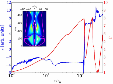
Figure 16: Entropy (blue) and Lorentz factor (red) along a velocity streamline of the jet in the B2-3D-hr simulation (note different y-axes). The inset shows the bottom-right panel of Fig. 13, and the white line shows the particular chosen velocity streamline. Entropy increases and velocity decreases at $r\sim 100r_{0}$ and $\sim 200r_{0}$, the locations of the first and second conical shocks. Outside the shocks, the Lorentz factor smoothly increases, reflecting the magnetic acceleration of the jets. The sharp jumps in the entropy and Lorentz factor reveal and confirm the presence of conical shocks. Note that at $r\sim 250r_{0}$, the streamline enters a sub-fast region in which 3D magnetic instabilities dissipate magnetic energy into thermal energy, as evidenced by a temporary increase in the entropy of the streamline (see text for more details).

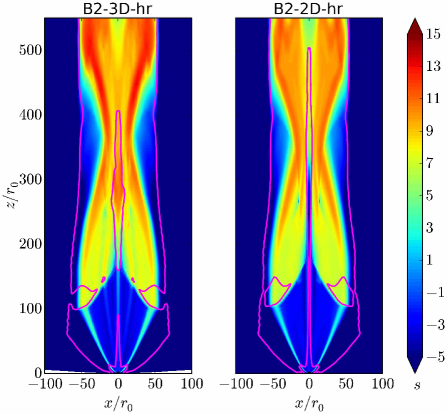
Figure 17: 2D entropy contours (arbitrary units) of models B2-3D-hr (left panel) and B2-2D-hr (right panel) at the final snapshot of the B2-3D-hr simulation ($t\approx 700r_{0}/c$). The magenta lines show the position of the fast magnetosonic surface in both panels. The entropy maps of these two models are almost identical. This shows that energy dissipation in the 2D and 3D runs is essentially the same, so there is no large contribution from 3D instabilities. There is a small fraction of energy that could be dissipated in the sub-fast region that develops along the jet axis a few $\times 10^{2}r_{0}$ away from the central object in the 3D-hr run (left panel) and also the 3D run. Since most of the jet power travels along the jet edges, energy contribution of the sub-fast region is quite small.

4 Discussion

How relativistic jets dissipate a large fraction of their energy and convert it to radiation remains an important unsolved problem in high-energy astrophysics. Magnetized relativistic jets are prone to various instabilities including the magnetic kink instability, which is thought to be the primary candidate for dissipation in the jets (e.g., Spruit, Daigne & Drenkhahn, 2001; Lyutikov & Blandford, 2003; Giannios & Spruit, 2006; Moll, Spruit & Obergaulinger, 2008; Narayan, Kumar & Tchekhovskoy, 2011; Sironi, Petropoulou & Giannios, 2015). Jets in nature propagate over as many as 10 orders of magnitude in distance. This gives plenty of room for the instabilities to develop. Studying their development is an inherently 3D multi-scale problem that involves jet acceleration, collimation and interaction with the ambient medium. Different elements of this problem have been studied extensively via numerical simulations (e.g., Nakamura, Li & Li, 2007; McKinney & Blandford, 2009; Mizuno et al., 2012; Mignone et al., 2013; Guan, Li & Li, 2014; Porth & Komissarov, 2015; Bromberg & Tchekhovskoy, 2016; Tchekhovskoy & Bromberg, 2016; Singh, Mizuno & de Gouveia Dal Pino, 2016).

To make numerical studies of jets feasible, the standard approach is to reduce the dynamic range covered in simulations. Primarily because of this, the development of magnetic instability in jets has been extensively studied via 3D numerical MHD simulations that inject relativistic jets at large distances from the central compact object (Guan, Li & Li, 2014, e.g.,). A crucial parameter that determines jet stability is the magnetic pitch, or the ratio of longitudinal to transverse magnetic field components in the jet, $B_{p}/B_{\varphi}$ (see, e.g., Appl, Lery & Baty, 2000; Guan, Li & Li, 2014). Unlike many previous studies, where the magnetic pitch is a free parameter set by the “jet injection” boundary condition (Nakamura, Li & Li, 2007, e.g.,), we follow a different approach and initiate the jets the way nature does it, via the rotation of the central magnetized compact object (Blandford & Znajek, 1977; Hawley & Krolik, 2006; McKinney & Blandford, 2009; Komissarov et al., 2007; Tchekhovskoy, McKinney & Narayan, 2009; Tchekhovskoy, Narayan & McKinney, 2010a, b; Tchekhovskoy, Narayan & McKinney, 2011; Bromberg & Tchekhovskoy, 2016; Tchekhovskoy & Bromberg, 2016, e.g.,). This fixes the magnetic pitch to its natural value and allows us to study jet stability from first principles.

The kink instability triggers magnetic reconnection, which in turn leads to magnetic energy dissipation that could readily explain the bright multi-wavelength emission attributed to jets in various astrophysical systems ranging from short- and long-duration GRBs to AGN, tidal disruption events, and pulsar wind nebulae (Bromberg & Tchekhovskoy, 2016). The focus of this work is on extending the simulated dynamic range and, for the first time in the context of AGN jets, following the jets from their birth at the surface of the central compact object out to their interaction with the external medium (ISM).

In the first attempt at addressing this important problem, we adopt several simplifying assumptions that make the current-generation of our simulations computationally feasible: (i) we reduce the range of jet acceleration and collimation zone from $5{-}6$ orders of magnitude in nature down to $2$ orders of magnitude; (ii) we consider powerful jets that propagate the fastest in order to reduce the computational cost; (iii) we ignore gravity because it is not important at large distances where the instabilities take place and over the short time-scales simulated; (iv) we assume a monopolar magnetic field geometry at the central object; and (v) we approximate ambient medium via an initially prescribed density profile. While this work focuses on relativistic AGN jets, our results can be extended to other astrophysical systems with relativistic jets.

In this paper we studied relativistic jets that interact with the ambient medium in order to understand how and whether this interaction triggers jet energy dissipation. We did this via 2D and 3D relativistic MHD simulations with different external medium density distributions (see Tables 2–3 and Fig. 1). Considering different types of ambient medium allowed us to study two distinct classes of jets: headed and headless jets. Headed jets drill through and push the ambient medium. Headless jets propagate through a previously evacuated funnel. Although this distinction is not always clear-cut (since realistic astrophysical systems could involve a combination of these two types of jets), considering the two limiting cases helps us to elucidate the jet physics in the simplest circumstances.

4.1 Headed jets

Headed jets were found to be unstable in previous 3D MHD simulations of mildly relativistic jets that followed them from the central object (Bromberg & Tchekhovskoy, 2016; Tchekhovskoy & Bromberg, 2016). These simulations did not set the magnetic pitch as an initial condition: the pitch was self-consistently determined by the rotation of the central object. These authors found that a stable jet that interacts with a density profile, $\rho\propto r^{-\alpha}$ with $\alpha\mathrel{\hbox{\hbox to0.0pt{\hbox{\lower 4.0pt\hbox{$\sim$}}\hss}\hbox{$<$}}}2$, tends to turn unstable as it propagates farther away from the compact object (Tchekhovskoy & Bromberg, 2016). However, if this jet interacts with a profile with $\alpha\mathrel{\hbox{\hbox to0.0pt{\hbox{\lower 4.0pt\hbox{$\sim$}}\hss}\hbox{$>$}}}2$, then it would remain stable (see also Porth & Komissarov 2015 who considered stability of headless jets as a function of the power-law index of the ambient pressure profile). These conclusions were found for mildly relativistic jets, $\Gamma\sim 1$.

We found that headed jets that run into a density break from steep to flat density profile (we adopt for the flat profile $\alpha=1$, as suggested observationally, Russell et al. 2015) switch from parabolic to cylindrical shape. Recent observations of jets in the M87 galaxy (Asada & Nakamura, 2012) and several other AGN (Algaba et al., 2016; Tseng et al., 2016) also indicate a switch in the geometry of the jet close to the Bondi radius. We note that whereas observations prefer a conical jet shape beyond the Bondi radius, our simulated jets tend to collimate into cylinders. It is possible that this difference comes from the neglect of gravity in our simulations: without gravity, the hot jet exhaust flows back along the jet and equilibrates the confining pressure. Because the pressure is uniform along the jet, it collimates the jet into a cylinder. The effect of gravity would be to gravitationally stratify the confining gas. This would lead to pressure decreasing with increasing distance from the source and possibly resulting in a finite opening angle of the jet.

We also found that at the transition between the two geometries the jets recollimate, i.e., abruptly bend on to the jet axis. At this recollimation point, the jets exhibit a ‘pinch’ or a ‘waist’ (see also Bromberg & Tchekhovskoy 2016). Such places in the jet are natural sites for the development of the kink instability: because the instability growth time-scale is essentially the sound crossing time across the jet, the natural place for the instability to develop is where the jet cross-section is the smallest, i.e., near the recollimation point. Indeed, we find that at the recollimation point, our jets develop an internal magnetic kink instability that twists the internals of the jet on to itself and generates current sheets that dissipate $\mathrel{\hbox{\hbox to0.0pt{\hbox{\lower 4.0pt\hbox{$\sim$}}\hss}\hbox{$>$}}}50$% of jet magnetic energy into heat over a factor of few in distance.

Dissipation in jets occurs on the small, resistive scales. These dissipative scales in jets in nature are small compared to the jet size. In fact, they are so much smaller than the size of the numerical cells in our simulations that it is unrealistic to hope to capture them in a global simulation. In fact, while we would like to include non-ideal effects into our simulations explicitly, we would not be able to do so realistically: any dissipative scale we would include would still be much larger than in nature. Because of this, we do no include explicit resistivity into our simulations. The numerical scheme instead relies on the fact that when two oppositely oriented magnetic field lines get squished into a single numerical cell, they annihilate and their energy gets converted into heat. So, our simulations have a dissipative scale length comparable to the grid cell size. The hope is that if the numerical resolution is high enough, the dissipative scale becomes so much smaller than the global scales involved in the problem that it no longer matters. We studied the convergence of our simulations with numerical resolution in 2D and 3D by doubling the resolution in every dimension. We found that in 3D a higher resolution leads to a larger amount of energy dissipated by the kink instability (Sec. 3.1.4). This indicates that the dissipation process is robust and the fraction of magnetic energy that is dissipated into heat can be of order unity. As more computational resources become available, in the future we will attempt to carry out simulations at even higher resolutions. This will help us to answer an important question of whether the simulation results converge to a well-defined answer in the infinitely high resolution limit that is closest to reality in the sense of the dissipation length scale being small. Local kinetic (e.g., Sironi, Petropoulou & Giannios, 2015; Sironi, Giannios & Petropoulou, 2016; Liu et al., 2016) and resistive MHD (e.g., Del Zanna et al., 2016) simulations could inform us about the best way of including physical dissipation in global jet models.

The recollimation point moves much slower than the jet fluid. It is tempting to associate the recollimation point and the associated dissipation with quasi-stationary or “slow” moving features in the core of the M87 jet (e.g., HST-1 and other knots; Biretta, Sparks & Macchetto, 1999; Meyer et al., 2013) and jets in other systems (Jorstad et al., 2005; Lister et al., 2013; Cohen et al., 2014). At larger radii, our jets develop large-scale bends and asymmetries characteristic of the external kink instability and powerful Fanaroff & Riley (1974) type II AGN such as Cygnus A (see also Tchekhovskoy & Bromberg, 2016).

An important new element of our work is the presence of acceleration and collimation zone extending from the central compact object to the ISM. This allows our jets to reach super-fast magnetosonic velocities. Because of this the jet outruns the fast magnetosonic waves, ensuring that no signals can propagate backwards to the central compact object, just as expected in nature (see Sec. 3.1.1 for discussion). Once such a super-fast jet runs into the ISM, it develops a shock or a series of shocks, which decrease its velocity. We find that the fraction of electromagnetic energy flux dissipated via such shocks is rather low in headed jets, $\mathrel{\hbox{\hbox to0.0pt{\hbox{\lower 4.0pt\hbox{$\sim$}}\hss}\hbox{$<$}}}5$% (see Appendix A). Nevertheless, the shocks slow down the flow substantially, allowing for the instabilities to proceed in the first place (see Section 3.1.4). Most of the energy flux, $\mathrel{\hbox{\hbox to0.0pt{\hbox{\lower 4.0pt\hbox{$\sim$}}\hss}\hbox{$>$}}}50$%, is dissipated through magnetic reconnection in the current sheets formed by the internal magnetic kink instability ; there is evidence in Figs. 4 and 9 that magnetic field lines are perturbed, which reflects both the emergence of irregular magnetic fields in the jets and the large-scale deviations of the jets out of the image plane, both caused by the 3D magnetic kink instability and ideal locations for magnetic reconnection to occur.

Interestingly, in addition to dissipation co-spatial with the recollimation feature, our headed jets develop an unstable, sub-fast magnetosonic region near the jet axis at distances comparable to the location of the density break in the ambient density (see Fig. 3 and Section 3.1.4). It is tantalizing that this sub-fast region can even in some cases extend to distances smaller than the location of the density break, and can appear even in the cases when there is no density break (see Fig. 2). This could provide a potential source for energy dissipation along the central region of the jet (Bromberg & Tchekhovskoy, 2016). Even though the amount of energy flowing through and dissipated in this region is small, the axial dissipation associated with it could power the low-frequency jet radio emission and contribute to the formation of the flat radio spectrum of jetted AGN. Intriguingly, this feature appears to be robust, as we find an indication for a similar feature in our headless jets, as we discuss below. Our simulations suggest that our jets are initially slow at the spine and fast at the edge, and are surrounded by a slower sheath. With increasing distance, as the jet accelerates, the relative fraction of jet cross-section occupied by the central slow spine shrinks, which might lead to a more uniform transverse luminosity profile of the jet. Our findings might have relevant connections with the observational evidence of limb brightening in Markarian 501, M87 and other jets (e.g. Giroletti et al., 2004; Kovalev et al., 2007).

4.2 Headless jets

To model headless jets, we carved out in the ambient gas a very low-density smooth polar escape route for a jet, as seen in the middle panel of Fig. 1 (model B). This allows the jets to propagate freely along the polar region without the need to push any external medium, in contrast to our study on headed jets. Our headless jets easily accelerate to high Lorentz factors and maintain a parabolic-like shape. The jets remain essentially axisymmetric. We find that the electromagnetic energy transforms to kinetic energy, and the jets accelerate to a Lorentz factor $\Gamma\sim 10$ over several orders of magnitude in distance, without undergoing significant internal energy dissipation. There is no indication of magnetic kink instabilities in these jets. This is consistent with the findings of McKinney & Blandford (2009), who found their jets also to be stable in a similar scenario.

We introduced the external medium for headless jets by changing the shape of our funnel into a dense cylinder, as seen in the right panel of Fig. 1 (model B2). We made this change approximately two orders of magnitude away from the central object. As the jet expands and propagates, it accelerates and loses lateral causal contact before it encounters the cylindrical part of the funnel. Once the jet hits the cylindrical funnel walls, it develops a conical shock that brings the jet into lateral causal contact and increases the toroidal magnetic field strength. The stronger toroidal magnetic field causes the jet to pinch and recollimate toward the jet axis, where it goes through another conical shock before expanding again. This process repeats, leading to a wavy jet featuring many recollimation points with a rather regular spacing (see Fig. 14). The recollimation points propagate very slowly, with $v\mathrel{\hbox{\hbox to0.0pt{\hbox{\lower 4.0pt\hbox{$\sim$}}\hss}\hbox{$<$}}}0.1c$. These points move because the funnel walls, not completely rigid, are pushed by the jet and move extremely slowly, making the situation not completely static and thus allowing the recollimation points to also move, albeit with a small velocity. The jet remains essentially axisymmetric. At the expansion and contraction of the jet between the recollimation points, two or more conical shocks are observed.

Lyubarsky (2009); Komissarov, Porth & Lyutikov (2015) studied a 2D evolution of a magnetized jet confined by a medium of a flat pressure profile. They found a breathing ($m=0$) mode in the jet similar to what we observe in our model B2 jet. These works considered jets in lateral causal contact with the ambient medium: their Lorentz factor smoothly increased (decreased) in response to expansion (contraction) of the jet radius. Our simulations are the first 3D study of jet breathing mode. They show that this mode can naturally develop as a result of jet interaction with an obstacle in the ambient medium. Unlike the above works, our jets drop out of lateral causal contact by the time they become reconfined by the obstacle in the ambient medium. As a result, jet radius oscillations are accompanied by conical shocks that keep bringing the jet into lateral causal contact and can even lead to a 3D kink instability near the jet axis (see below). In contrast to previous works, we find that the jet accelerates both at the expansion and at the contraction. We suggest that the acceleration occurs in both cases due to the sensitivity of the Lorentz factor to the poloidal curvature of the magnetic field lines (Tchekhovskoy, McKinney & Narayan, 2008). Mizuno et al. (2015) found a related breathing mode in their 2D numerical simulations of over-pressured jets. As their jets adjusted to the ambient medium, they developed shocks and rarefactions (for details of rarefaction acceleration, see, Aloy & Rezzolla, 2006; Mizuno et al., 2008; Tchekhovskoy, Narayan & McKinney, 2010b; Komissarov, Vlahakis & Königl, 2010, e.g.,). However, Mizuno et al. (2015) assume that initially the relativistic jet is kinematically dominated for all values of the magnetic field they consider. In contrast, our jet is initially magnetically dominated. Future work will explore the physics of jet acceleration in our simulations.

Recently, a scenario in which a jet encounters an abrupt flattening of the pressure profile at some radius, which would be somewhat analogous to our model B2, has been presented by Levinson & Globus (2017). These authors find strong jet radius oscillations upon transition from the steeper to the flatter pressure profile, which we also find as our funnel transitions to a cylindrical shape. However, as mentioned before, in our 2D and 3D numerical simulations we find jet acceleration both at the expansion and contraction (instead of only at the contraction) and resolve the presence of conical shocks, which efficiently decelerate the jet. This highlights the importance of accounting for discontinuities and shocks in the jet, which can significantly affect the jet Lorentz factor.

In contrast to headed jets, we find that headless jets are stable to 3D kink instability. The main reason is that headed jets show a larger toroidal to poloidal magnetic field ratio, a steep poloidal field profile, and they are slower, whereas headless jets show a smaller toroidal to poloidal magnetic field ratio, a shallower poloidal field profile, and they are faster since they do not have to push against a large ambient density (e.g., Mizuno et al., 2012; Bromberg & Tchekhovskoy, 2016). These factors affect the growth of kink instability, making it grow very slowly for headless jets.

The lack of 3D instabilities does not mean that energy dissipation does not occur. We find that headless jets that propagate in a smooth low-density funnel convert very little magnetic and kinetic energy to internal energy (model B). However, when we abruptly change our funnel to be cylindrical (model B2), the jets develop conical shocks at which internal energy increases. A conical shock abruptly slows down the jet, decreasing its kinetic energy. This energy is almost equally shared towards an increase in electromagnetic energy, since the shock compresses the magnetic field, and towards an increase in internal energy. The level of energy dissipation is modest, $\sim 10$ per cent of the total jet power at the first conical shock. This level is lower than for headed jets, where the kink instability dissipates more energy, and will likely be even lower for jets at higher magnetization than we considered (e.g., Mimica, Giannios & Aloy, 2010; Narayan, Kumar & Tchekhovskoy, 2011).

Although we have been able to resolve numerically only a few conical shocks, we expect that many more of these conical shocks develop if we follow the jet out to larger scales, as suggested by Fig. 14. A sequence of many such shocks would result in a higher dissipation efficiency. It is tempting to associate a sequence of such dissipative shocks with the sequence of essentially equidistant knots seen in the M87 jet starting at the HST-1 knot (e.g., Meyer et al., 2013). In contrast to headed jets, our cylindrical headless jets can dissipate energy over a large range of distance so long as they maintain their cylindrical shape. We note that our jet is aligned relative to the cylindrical funnel. A misaligned jet (or a non-axisymmetric external medium) would likely prevent the development of a long sequence of shocks over distance and may develop additional instabilities.

Somewhat similar to the headed jets, in addition to energy dissipation at the location of conical shocks, there is a hint that some dissipation could be occurring along the jet axis via internal 3D magnetic kink instabilities in a sub-fast region (see Section 3.3.5). This region does not develop for model B, since its jet interacts with a very low-density ambient medium, but it develops for model B2, where the funnel turns cylindrical and causes conical shocks to form. This unstable region could be a side-product of the conical shocks, which slow down the jet fluid and increase the strength of the toroidal magnetic field, thereby encouraging the MHD instabilities to develop and additionally dissipate the electromagnetic flux. Furthermore, we see indications that at very late times this unstable sub-fast region could even extend to distances a bit smaller than the location of the cylindrical transition, which could provide a potential site for energy dissipation along the central region of the jet. Although small jet energy flux (internal energy flux at a level of a percent of the total jet energy flux) travels through the unstable region along the jet axis (most of the energy flows along the jet edges), the additional axial dissipation could be a promising mechanism for forming the low-frequency radio emission of flat radio spectrum jetted AGN.

5 Conclusions

We have performed a suite of fully 3D relativistic MHD simulations at various resolutions that follow two types of jets from the compact object: (i) headed jets, which interact with the ambient medium and push it out of the way in order to propagate, and (ii) headless jets, which propagate freely through a previously evacuated very low-density funnel (Bromberg & Tchekhovskoy, 2016). The jets are launched self-consistently via the rotation of a magnetized compact object and are followed for about 3 orders of magnitude in distance.

We find that as the headed jets encounter a shallower density profile, they recollimate and pinch toward the axis and succumb to a magnetic kink instability ($m=1$ mode). This instability triggers strong, concentrated energy dissipation localised within an order of magnitude in distance of the location of the density profile break. The result is a slowly propagating recollimation point accompanied with dissipation, which could be associated with the slowly moving or stationary features observed in AGN jets.

Headless jets that encounter a sudden change in the shape of the low-density funnel through which they propagate, do not exhibit strong magnetic kink instabilities. Instead, they dissipate energy at essentially equidistant conical shocks that form as the jet develops a violent breathing ($m=0$) mode in an attempt to come to terms with the new shape of the confining funnel. In contrast to headed jets, dissipation in headless jets, although less efficient, can occur over a large range of distances so long as the funnel retains its shape. Such a series of equidistant shocks could correspond to the series of equidistant knots seen in the M87 jet (e.g., Meyer et al., 2013).

In both types of jets, a sub-fast unstable narrow region along the jet axis develops close to (and in some cases before) the location of the density profile break. This instability could light up helical structures near the jet axis and account for several, apparently helical threads in the jet of M87 upstream of HST-1 seen in a space-VLBI image with RadioAstron and a large global-VLBI array taken at 18cm (Savolainen et al., in preparation).

Among the simplifications of our numerical simulations, we have considered high-power jets, since they propagate the fastest in order to reduce the computational cost. In the future, we plan to extend our work to lower jet powers, and to increase the spatial range and duration of our simulations. We will also study the dependence of our results on the value of the jets’ initial magnetization, currently the same for all our simulations, which could have important consequences for the development of the magnetic kink instability and the recollimation structures.

Appendix A Numerical convergence for 2D models of jets

Whereas in the main text we focused on the numerical convergence of 3D models, in this Appendix we present the results of numerical convergence for the 2D models. This allows us to compare the levels of dissipation between 2D and 3D simulations and thereby to determine the dissipation regions that likely represent physically-motivated dissipation sites.

In Fig. 18 we present the different energy fluxes as described in Section 3.1.4 for all our models. Instead of presenting only 3D and 2D simulations as we did in Figs. 8, 10 and 15, in Fig. 18 we also present the results from our higher-resolution 2D simulations, 2D-hr and 2D-vhr.

As can be seen in Fig. 18, in model A (top-left), as we increase the 2D resolution, the internal energy flux decreases. Since in the A-3D simulation the internal energy flux is at the level of the A-2D simulation, we ascribe the energy dissipation seen in the A-3D simulation to insufficient resolution. For models A2 (top-middle), A2x3 (top-right) and A1 (bottom-left), the internal energy flux decreases as we increase the 2D resolution. However, the level of internal energy flux in the 3D runs of these simulations exceeds that of all 2D runs at different resolutions. This suggests that in these 3D models the dissipation is physical. In fact, a 3D convergence study, shown in the right panel of Fig. 8, demonstrates that at a higher-resolution 3D simulation A2-3D-hr shows an even larger internal energy flux than the fiducial resolution simulation A2-3D. This indicates that the dissipation is robust and consistent with being due to the 3D magnetic kink instability.

In addition to energy dissipation in the current sheets produced by the internal kink instability, we identify another potential dissipation site: one or several shocks through which our super-fast magnetosonic jets learn about the presence of the ambient medium. They have to do so through shocks because by the time our jets reach the ambient medium, they move at a super-fast magnetosonic velocity and therefore do not know anything about the impending collision. The shocks are accompanied by a spike in the internal energy. They are easiest to identify in the highest resolution simulations, in which the value of the internal energy is the most accurate: at $r\sim 100r_{0}$ in the right-most panel in Fig. 8, at $r\sim 150r_{0}$ in simulations A-2D-hr/A-2D-vhr, A2-2D-hr/A2-2D-vhr, and A2x3-2D-hr/A2x3-2D-vhr in the top row of panels in Fig. 18. As the resolution increases, the fraction of energy carried in the form of heat (or internal energy) decreases in the post-shock region, becoming as low as $\mathrel{\hbox{\hbox to0.0pt{\hbox{\lower 4.0pt\hbox{$\sim$}}\hss}\hbox{$<$}}}5$% at the highest resolutions. This demonstrates that the dissipation by these shocks is sub-dominant to the dissipation by the internal kink instability, which converts as much as $50$% of the total energy flux into heat. In future work, we will investigate how the fraction of the total jet power dissipated at these shocks depends on the jet magnetization and on the dynamical range accessible to the jets in the collimation and acceleration region: it is plausible that if the jets had a chance to accelerate to higher values of the Lorentz factor, they would have reached the shock at a lower value of magnetization and would be more readily able to heat up (e.g., Mimica, Giannios & Aloy, 2010).

For model B in the bottom-middle panel of Fig. 18, it is clear that increasing the 2D resolution essentially reduces the internal energy flux to zero. Thus, the internal energy flux increase seen in B-3D is due to insufficient resolution. Also, a 3D convergence study showed a significant decrease in the internal energy flux for the simulation B-3D-hr (top-right panel of Fig. 15). Finally, as seen in the bottom-right panel of Fig. 18, model B2 shows almost identical levels of energy fluxes for different 2D resolution runs, indicating that all our simulations show convergence. We found the same conclusion with our 3D convergence study for this model in the bottom-right panel of Fig. 15.

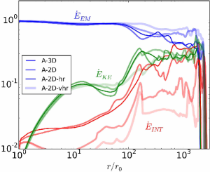
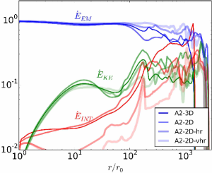
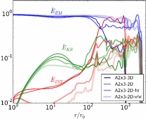
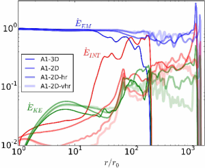
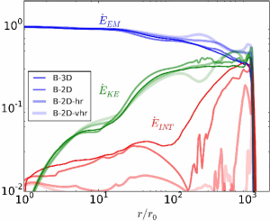
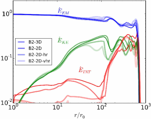
Figure 18: Different components of the energy flux (see labels) for 3D and 2D simulations of model A (top-left, $t\approx 2700r_{0}/c$), A2 (top-middle, $t\approx 3000r_{0}/c$), A2x3 (top-right , $t\approx 3400r_{0}/c$), A1 (bottom-left, $t\approx 2800r_{0}/c$), B (bottom-middle, $t\approx 1200r_{0}/c$) and B2 (bottom-right, $t\approx 700r_{0}/c$). All quantities are calculated at the final snapshots of the simulations, except for models B and B2, where we have used the final snapshot of the 3D-hr simulations, respectively (see Table 3). The energy fluxes have been normalized to the value of the total energy flux at $r=r_{0}$. The distance at which the energy flux drops to zero marks the location of the jet head. We ascribe the energy dissipation and internal energy flux increase seen in models A-3D and B-3D due to insufficient numerical resolution. However, the internal energy flux increase seen in models A2, A2x3 and A1 exceeds the level seen in 2D runs. Model B2-3D shows a nice convergence with 2D runs. For 3D convergence studies see Figs. 8 and 15.

Appendix B 2D simulations of models B and B2

We show 2D runs at different resolutions of model B and B2, see Figs. 19 and 20, respectively. The 2D jets propagate at similar velocities at different 2D resolutions and their shapes appear similar, although as we increase the $N_{\theta}$-resolution we are able to better resolve the interface between the jet and the pre-existing funnel and thus the jet appears a bit wider. The 2D jets appear also very similar to the 3D jets of these models seen in Figs. 12 and 13. As also seen in our 3D convergence study (Fig. 13), when we increase the 2D resolution of our model B2 runs, we are able to better resolve multiple shocks.

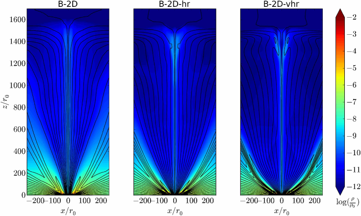
Figure 19: Density contours of 2D simulations of model B: B-2D (left), B-2D-hr (middle) and B2-vhr (right panel) at the final snapshot ($t\approx 1500r_{0}/c$; same scales and colorbar in all panels). Black lines show magnetic flux surfaces. The jet in model B propagates freely in a pre-existing funnel and it expands as it travels. Different 2D resolutions show similar jet propagation velocities and similar jet shapes, although as we increase 2D resolution the jet becomes wider due to the increase of the $N_{\theta}$-resolution and our enhanced ability to resolve the interface between the jet and the pre-existing funnel.

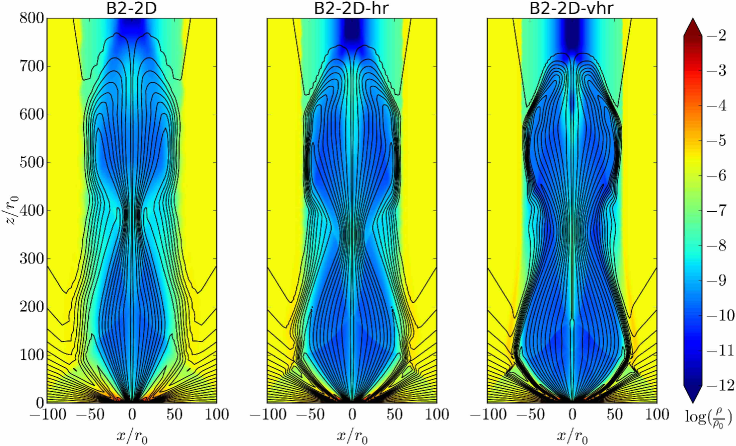
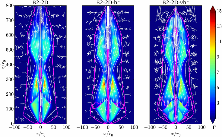
Figure 20: Density contours (top panels) and Lorentz factor contours (bottom panels) of model B2: B2-2D (left), B2-2D-hr (middle) and B2-vhr (right panel) at the same time ($t\approx 700r_{0}/c$; same scales in all panels, same density and Lorentz factor colorbars for the top and bottom panels, respectively). Black lines show magnetic flux surfaces. The jet in model B2 propagates in a pre-existing funnel that becomes cylindrical at $z=80r_{0}$. The presence of shocks is evident by inspecting the Lorentz factor plots. 2D simulations show multiple shocks, which become better resolved at higher resolution. Different 2D resolutions show similar jet propagation velocities and similar jet shapes, although as we increase 2D resolution the jet becomes wider due to the increase of the $N_{\theta}$-resolution and our enhanced ability to resolve the interface between the jet and the pre-existing funnel.

References

- Algaba et al. (2016) Algaba J.-C., Nakamura M., Asada K., Lee S.-S., 2016, ArXiv:1611.04075
- Aloy et al. (2000) Aloy M. A., Müller E., Ibáñez J. M., Martí J. M., MacFadyen A., 2000, ApJ, 531, L119
- Aloy & Rezzolla (2006) Aloy M. A., Rezzolla L., 2006, ApJ, 640, L115
- Appl, Lery & Baty (2000) Appl S., Lery T., Baty H., 2000, A&A, 355, 818
- Asada & Nakamura (2012) Asada K., Nakamura M., 2012, ApJ, 745, L28
- Begelman (1998) Begelman M. C., 1998, ApJ, 493, 291
- Beskin & Nokhrina (2006) Beskin V. S., Nokhrina E. E., 2006, MNRAS, 367, 375
- Biretta, Sparks & Macchetto (1999) Biretta J. A., Sparks W. B., Macchetto F., 1999, ApJ, 520, 621
- Blandford & Znajek (1977) Blandford R. D., Znajek R. L., 1977, MNRAS, 179, 433
- Bromberg & Tchekhovskoy (2016) Bromberg O., Tchekhovskoy A., 2016, MNRAS, 456, 1739
- Cohen et al. (2014) Cohen M. H. et al., 2014, ApJ, 787, 151
- De Colle et al. (2012) De Colle F., Ramirez-Ruiz E., Granot J., Lopez-Camara D., 2012, ApJ, 751, 57
- De Villiers et al. (2005) De Villiers J.-P., Hawley J. F., Krolik J. H., Hirose S., 2005, ApJ, 620, 878
- Del Zanna et al. (2016) Del Zanna L., Papini E., Landi S., Bugli M., Bucciantini N., 2016, MNRAS, 460, 3753
- Fanaroff & Riley (1974) Fanaroff B. L., Riley J. M., 1974, MNRAS, 167, 31P
- Fender, Belloni & Gallo (2004) Fender R. P., Belloni T. M., Gallo E., 2004, MNRAS, 355, 1105
- Fielding et al. (2016) Fielding D., Quataert E., McCourt M., Thompson T. A., 2016, ArXiv:1606.06734
- Frail et al. (2001) Frail D. A., et al., 2001, ApJ, 562, L55
- Gammie, McKinney & Tóth (2003) Gammie C. F., McKinney J. C., Tóth G., 2003, ApJ, 589, 444
- Gammie, Shapiro & McKinney (2004) Gammie C. F., Shapiro S. L., McKinney J. C., 2004, ApJ, 602, 312
- Gaspari, Ruszkowski & Sharma (2012) Gaspari M., Ruszkowski M., Sharma P., 2012, ApJ, 746, 94
- Ghisellini et al. (2014) Ghisellini G., Tavecchio F., Maraschi L., Celotti A., Sbarrato T., 2014, Nature, 515, 376
- Giannios & Spruit (2006) Giannios D., Spruit H. C., 2006, A&A, 450, 887
- Giroletti et al. (2004) Giroletti M. et al., 2004, ApJ, 600, 127
- Guan, Li & Li (2014) Guan X., Li H., Li S., 2014, ApJ, 781, 48
- Hawley & Krolik (2006) Hawley J. F., Krolik J. H., 2006, ApJ, 641, 103
- Ishibashi & Fabian (2012) Ishibashi W., Fabian A. C., 2012, MNRAS, 427, 2998
- Jorstad et al. (2005) Jorstad S. G., et al., 2005, AJ, 130, 1418
- Kohler, Begelman & Beckwith (2012) Kohler S., Begelman M. C., Beckwith K., 2012, MNRAS, 422, 2282
- Komissarov et al. (2007) Komissarov S. S., Barkov M. V., Vlahakis N., Königl A., 2007, MNRAS, 380, 51
- Komissarov, Porth & Lyutikov (2015) Komissarov S. S., Porth O., Lyutikov M., 2015, Computational Astrophysics and Cosmology, 2, 9
- Komissarov, Vlahakis & Königl (2010) Komissarov S. S., Vlahakis N., Königl A., 2010, MNRAS, 407, 17
- Kovalev et al. (2007) Kovalev Y. Y., Lister M. L., Homan D. C., Kellermann K. I., 2007, ApJ, 668, L27
- Levinson & Globus (2017) Levinson A., Globus N., 2017, MNRAS, 465, 1608
- Li et al. (2015) Li Y., Bryan G. L., Ruszkowski M., Voit G. M., O’Shea B. W., Donahue M., 2015, ApJ, 811, 73
- Lister et al. (2011) Lister M. L. et al., 2011, ApJ, 742, 27
- Lister et al. (2013) Lister M. L. et al., 2013, AJ, 146, 120
- Liu et al. (2016) Liu Y.-H., Hesse M., Guo F., Daughton W., Li H., 2016, ArXiv:1605.05654
- López-Cámara et al. (2013) López-Cámara D., Morsony B. J., Begelman M. C., Lazzati D., 2013, ApJ, 767, 19
- Lyubarskii (1999) Lyubarskii Y. E., 1999, MNRAS, 308, 1006
- Lyubarsky (2009) Lyubarsky Y., 2009, ApJ, 698, 1570
- Lyutikov & Blandford (2003) Lyutikov M., Blandford R., 2003, ArXiv Astrophysics e-prints
- McKinney (2006) McKinney J. C., 2006, MNRAS, 368, 1561
- McKinney & Blandford (2009) McKinney J. C., Blandford R. D., 2009, MNRAS, 394, L126
- Meliani, Keppens & Giacomazzo (2008) Meliani Z., Keppens R., Giacomazzo B., 2008, A&A, 491, 321
- Meyer et al. (2013) Meyer E. T., Sparks W. B., Biretta J. A., Anderson J., Sohn S. T., van der Marel R. P., Norman C., Nakamura M., 2013, ApJ, 774, L21
- Mignone et al. (2010) Mignone A., Rossi P., Bodo G., Ferrari A., Massaglia S., 2010, MNRAS, 402, 7
- Mignone et al. (2013) Mignone A., Striani E., Tavani M., Ferrari A., 2013, MNRAS, 436, 1102
- Mimica, Giannios & Aloy (2010) Mimica P., Giannios D., Aloy M. A., 2010, MNRAS, 407, 2501
- Mizuno et al. (2015) Mizuno Y., Gómez J. L., Nishikawa K.-I., Meli A., Hardee P. E., Rezzolla L., 2015, ApJ, 809, 38
- Mizuno et al. (2008) Mizuno Y., Hardee P., Hartmann D. H., Nishikawa K.-I., Zhang B., 2008, ApJ, 672, 72
- Mizuno, Hardee & Nishikawa (2014) Mizuno Y., Hardee P. E., Nishikawa K.-I., 2014, ApJ, 784, 167
- Mizuno et al. (2012) Mizuno Y., Lyubarsky Y., Nishikawa K.-I., Hardee P. E., 2012, ApJ, 757, 16
- Moll, Spruit & Obergaulinger (2008) Moll R., Spruit H. C., Obergaulinger M., 2008, A&A, 492, 621
- Morsony, Lazzati & Begelman (2007) Morsony B. J., Lazzati D., Begelman M. C., 2007, ApJ, 665, 569
- Murguia-Berthier et al. (2014) Murguia-Berthier A., Montes G., Ramirez-Ruiz E., De Colle F., Lee W. H., 2014, ApJ, 788, L8
- Nakamura & Asada (2013) Nakamura M., Asada K., 2013, ApJ, 775, 118
- Nakamura, Li & Li (2007) Nakamura M., Li H., Li S., 2007, ApJ, 656, 721
- Nakamura & Meier (2004) Nakamura M., Meier D. L., 2004, ApJ, 617, 123
- Narayan, Kumar & Tchekhovskoy (2011) Narayan R., Kumar P., Tchekhovskoy A., 2011, MNRAS, 416, 2193
- Narayan, Li & Tchekhovskoy (2009) Narayan R., Li J., Tchekhovskoy A., 2009, ApJ, 697, 1681
- Nemmen et al. (2012) Nemmen R. S., Georganopoulos M., Guiriec S., Meyer E. T., Gehrels N., Sambruna R. M., 2012, Science, 338, 1445
- Nemmen & Tchekhovskoy (2015) Nemmen R. S., Tchekhovskoy A., 2015, MNRAS, 449, 316
- Noble et al. (2006) Noble S. C., Gammie C. F., McKinney J. C., Del Zanna L., 2006, ApJ, 641, 626
- Panaitescu & Kumar (2002) Panaitescu A., Kumar P., 2002, ApJ, 571, 779
- Perucho et al. (2010) Perucho M., Martí J. M., Cela J. M., Hanasz M., de La Cruz R., Rubio F., 2010, A&A, 519, A41
- Porth & Komissarov (2015) Porth O., Komissarov S. S., 2015, MNRAS, 452, 1089
- Rawlings & Saunders (1991) Rawlings S., Saunders R., 1991, Nature, 349, 138
- Ressler et al. (2017) Ressler S. M., Tchekhovskoy A., Quataert E., Gammie C. F., 2017, MNRAS, 467, 3604
- Rossi et al. (2008) Rossi P., Mignone A., Bodo G., Massaglia S., Ferrari A., 2008, A&A, 488, 795
- Russell et al. (2015) Russell H. R., Fabian A. C., McNamara B. R., Broderick A. E., 2015, MNRAS, 451, 588
- Singh, Mizuno & de Gouveia Dal Pino (2016) Singh C. B., Mizuno Y., de Gouveia Dal Pino E. M., 2016, ApJ, 824, 48
- Sironi, Giannios & Petropoulou (2016) Sironi L., Giannios D., Petropoulou M., 2016, MNRAS, 462, 48
- Sironi, Petropoulou & Giannios (2015) Sironi L., Petropoulou M., Giannios D., 2015, MNRAS, 450, 183
- Spruit, Daigne & Drenkhahn (2001) Spruit H. C., Daigne F., Drenkhahn G., 2001, A&A, 369, 694
- Taylor et al. (2004) Taylor G. B., Frail D. A., Berger E., Kulkarni S. R., 2004, ApJ, 609, L1
- Tchekhovskoy (2015) Tchekhovskoy A., 2015, in Astrophysics and Space Science Library, Vol. 414, The Formation and Disruption of Black Hole Jets, Contopoulos I., Gabuzda D., Kylafis N., eds., p. 45
- Tchekhovskoy & Bromberg (2016) Tchekhovskoy A., Bromberg O., 2016, MNRAS, 461, L46
- Tchekhovskoy, McKinney & Narayan (2007) Tchekhovskoy A., McKinney J. C., Narayan R., 2007, MNRAS, 379, 469
- Tchekhovskoy, McKinney & Narayan (2008) Tchekhovskoy A., McKinney J. C., Narayan R., 2008, MNRAS, 388, 551
- Tchekhovskoy, McKinney & Narayan (2009) Tchekhovskoy A., McKinney J. C., Narayan R., 2009, ApJ, 699, 1789
- Tchekhovskoy, Narayan & McKinney (2010a) Tchekhovskoy A., Narayan R., McKinney J. C., 2010a, ApJ, 711, 50
- Tchekhovskoy, Narayan & McKinney (2010b) Tchekhovskoy A., Narayan R., McKinney J. C., 2010b, New Astronomy, 15, 749
- Tchekhovskoy, Narayan & McKinney (2011) Tchekhovskoy A., Narayan R., McKinney J. C., 2011, MNRAS, 418, L79
- Tseng et al. (2016) Tseng C.-Y., Asada K., Nakamura M., Pu H.-Y., Algaba J.-C., Lo W.-P., 2016, ApJ, 833, 288
- Vernaleo & Reynolds (2006) Vernaleo J. C., Reynolds C. S., 2006, ApJ, 645, 83
- Vernaleo & Reynolds (2007) Vernaleo J. C., Reynolds C. S., 2007, ApJ, 671, 171
- Yoon et al. (2011) Yoon D., Morsony B., Heinz S., Wiersema K., Fender R. P., Russell D. M., Sunyaev R., 2011, ApJ, 742, 25