Radiation enhancement and “temperature” in the collapse regime of gravitational scattering

Abstract

We generalize the semiclassical treatment of graviton radiation to gravitational scattering at very large energies $\sqrt{s}\gg m_{P}$ and finite scattering angles $\Theta_{s}$, so as to approach the collapse regime of impact parameters $b\simeq b_{c}\sim R\equiv 2G\sqrt{s}$. Our basic tool is the extension of the recently proposed, unified form of radiation to the ACV reduced-action model and to its resummed-eikonal exchange. By superimposing that radiation all-over eikonal scattering, we are able to derive the corresponding (unitary) coherent-state operator. The resulting graviton spectrum, tuned on the gravitational radius $R$, fully agrees with previous calculations for small angles $\Theta_{s}\ll 1$ but, for sizeable angles $\Theta_{s}(b)\leq\Theta_{c}=\mathcal{O}\left(1\right)$ acquires an exponential cutoff of the large $\omega R$ region, due to energy conservation, so as to emit a finite fraction of the total energy. In the approach-to-collapse regime of $b\to b_{c}^{+}$ we find a radiation enhancement due to large tidal forces, so that the whole energy is radiated off, with a large multiplicity $\langle N\rangle\sim Gs\gg 1$ and a well-defined frequency cutoff of order $R^{-1}$. The latter corresponds to the Hawking temperature for a black hole of mass notably smaller than $\sqrt{s}$.

1 Introduction

The investigation of transplanckian-energy gravitational scattering performed since the eighties [1, 2, 3, 4, 5, 6, 7, 8] and applied to the collapse regime [9, 10, 11, 12] has been recently revived at both classical [13] and quantum level [14, 15] with the purpose of describing the radiation associated to extreme energies and of gaining a better understanding of a possibly collapsing system. A bridge between the different approaches of [14] and [15] has also been devised [16].

Here we follow essentially the ACV path [5, 7, 8, 9], that is mostly an effective theory based on $s$-channel iteration (eikonal scattering) and motivated by the smallness of fixed-angle amplitudes in string-gravity [4] and by the high-energy dominance of the spin-2 graviton exchange, at small momentum transfers [1, 2, 3]. In fact, a key feature of eikonal scattering is that the large momentum transfers built up at fixed scattering angle (e.g. the Einstein deflection angle $\Theta_{E}\equiv 2R/b$) — $R\equiv 2G\sqrt{s}$ being the gravitational radius — is due to a large number $\langle n\rangle=Gs/\hbar\equiv{\alpha_{G}}\gg 1$ of single-hits with very small scattering angle $\theta_{m}\sim\hbar/bE$. By following these lines, ACV [8] proposed an all-order generalization of the semiclassical approach based on an effective action [17, 6], that allows in principle to compute corrections to the eikonal functions depending on the expansion parameter $R^{2}/b^{2}$ (by neglecting, in string-gravity, the smaller ones $\mathcal{O}\left(l_{s}^{2}/b^{2}\right)$ [5, 18] if $l_{P}<l_{s}\ll R$). In its axisymmetric formulation, the eikonal resummation reduces to a solvable model in one-dimensional radial space, that was worked out explicitly in [9]. Such reduced-action model allows to treat sizeable angles $R/b$, up to a singularity point $b_{c}=\sqrt{3\sqrt{3}/2}R$ where a branch point of critical index $3/2$ occurs in the action, as signal of a possible classical collapse.

The main purpose of the present paper is to extend the radiation treatment of [15, 19] to larger angles, by applying it to the ACV resummed eikonal, in order to achieve a comparable progress at radiation level. We shall then use it to study the extreme energy regime of a possible classical collapse $b\to b_{c}^{+}\sim R$.

Let us recall that the main qualitative understanding of [15], compared to previous approaches, was to disentangle the role of the gravitational radius $R$ in the radiation process. In fact, by superimposing the radiation amplitudes associated to the various eikonal exchanges and by combining the large number $\langle n\rangle\sim{\alpha_{G}}=ER$ of emitters with the relatively small energy fraction $\hbar\omega/E$, CCV found that the relevant variable becomes $\omega R$, which is thus needed to describe the interference pattern of the whole amplitude (sec. 2). In the present paper we follow the same strategy, by replacing the leading eikonal (single graviton exchange) by the resummed one (sec. 3).

There is, however, an important technical point to be understood. The single-exchange radiation amplitude was determined in [15, 19] by unifying in the $E\gg\hbar\omega$ regime the Regge region of large emission angles with the soft one. Such unifying relationship involves a simple rescaling $E\to\hbar\omega$ of the soft amplitude and is exact for single-graviton exchange. Here we wish to generalize the soft-based representation so obtained to all subleading eikonal contributions. No real proof of that statement is available yet. Nevertheless, we shall argue in sec. 3 that, starting from the H-diagram [7], the dominant Regge contributions are confined to the deep fragmentation regions of the incoming particles, thus allowing the approximate use of the unifying relationship mentioned before and of the ensuing soft-based representation.

By entering the large angle region, we meet the issue of energy conservation also [20, 21, 22, 23]. Indeed, the coherent radiation state obtained by the soft-based formulation treats the fast particles as sources and thus neglects, in a first instance, conservation constraints. By introducing them explicitly in sec. 4, we keep neglecting correlations that we argue to be small (sec. 3.4). However, the overall effect of energy conservation is quite important, in the large-angle region, because it introduces an exponential cutoff which — though preserving quantum coherence — plays a role similar to the temperature in a statistical ensemble.

The validity of the exponential behaviour and its role in approaching collapse are carefully discussed in sec. 4.3. The final outcome is that the whole energy is radiated off in the approach-to-collapse regime, by fixing the analogue of the Hawking temperature [24, 25] for our energetic sample of (coherent) radiation.

2 Graviton radiation in small-angle transplanckian
scattering

The approach to gravitational scattering and radiation advocated in [19] is based on a semiclassical approximation to the $S$-matrix of the form

$$S\simeq\exp\left\{2\mathrm{i}\hat{\delta}\Big{(}{\alpha_{G}},\frac{R}{b},a_{\lambda}(\vec{q})\Big{)}\right\}\;,$$ (2.1)

where the eikonal operator $\hat{\delta}$ is a function of the effective coupling ${\alpha_{G}}\equiv Gs/\hbar$ and of the angular variable $R/b$ (where $R\equiv 2G\sqrt{s}$ is the gravitational radius and $b$ the impact parameter) and a functional of the graviton step operators $a_{\lambda}(\vec{q})$ with helicity $\lambda$ and momentum $\vec{q}$.

The semiclassical form (2.1) was argued in [9] to be valid in the strong-gravity regime ${\alpha_{G}}\gg 1$ with $R\gg b\gg l_{s}>l_{P}$, where $l_{s}$ is the string length and $l_{P}\equiv\sqrt{\hbar G}$ the Planck length. This means that we are, to start with, in the transplanckian regime $\sqrt{s}\gg m_{P}=\hbar/l_{P}$ at small scattering angles $\Theta_{s}\simeq\Theta_{E}\equiv 2R/b$, where $\Theta_{E}$ is the Einstein deflection angle. Quantum corrections to (2.1) will involve the parameter $l_{P}^{2}/b^{2}$ (and $l_{s}^{2}/b^{2}$ if working within string-gravity) and will be partly considered later on.

The eikonal operator is then obtained by resumming an infinite series of effective diagrams which include virtual graviton exchanges and real graviton emissions, as will be shortly reviewed in the following. In the small-angle and low-density limit, it is composed by two terms: (i) a c-number phase shift $\delta_{0}$ generated by graviton exchanges between the external particles undergoing the scattering process; (ii) a linear superposition of creation and destruction operators which is responsible of graviton bremsstrahlung and associated quantum virtual corrections:

$$\hat{\delta}\Big{(}{\alpha_{G}},\frac{R}{b},a_{\lambda}(\vec{q})\Big{)}=\delta_{0}(b)+\int\frac{\mathrm{d}^{3}q}{\hbar^{3}\sqrt{2\omega}}\;\sum_{\lambda=\pm 2}\left[\mathfrak{M}_{\lambda}({\boldsymbol{b}},\vec{q})a^{\dagger}_{\lambda}(\vec{q})+\text{h.c.}\right]+\mathcal{O}\left(a_{\lambda}^{2}\right)\;,$$ (2.2)

where higher powers of $a_{\lambda}$ provide high-density corrections. This structure, which is valid for large impact parameters, i.e., for small values of the ratio $R/b\ll 1$, provides a unitary $S$-matrix describing the Einstein deflection of the scattered particles as well as its associated graviton radiation and its metric fields [9, 26] and time delays [27].

Actually, the subject of this paper is to extend the above picture to smaller impact parameters $b\sim R$ where the gravitational interaction becomes really strong and a gravitational collapse is expected on classical grounds. We will show that, decreasing the impact parameter $b$ up to some critical parameter $b_{c}\sim R$ of the order of the gravitational radius $R$, the form of the $S$-matrix maintains the form (2.1,2.2) with calculable corrections to both the phase shift $\delta_{0}$ (sec. 3.1) and to the emission amplitude $\mathfrak{M}$ (sec. 3.3). We shall then discuss in detail (sec. 4) what happens in the limit $b\to b_{c}$ from above.

2.1 Eikonal scattering

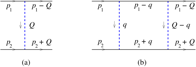
Figure 1: One- and two-rung effective ladder diagrams determining the elastic $S$-matrix in the eikonal approximation. Solid lines: on-shell external particles; dashed lines: eikonal gravitational exchanges.

ACV [7] have shown that the leading contributions to the high-energy elastic scattering amplitude $p_{1}+p_{2}\to p^{\prime}_{1}+p^{\prime}_{2}$ come from the $s$-channel iteration of soft-graviton exchanges, which can be represented by effective ladder diagrams as in fig. 1. The generic ladder is built by iteration (i.e., 4D convolution) of the basic rung

$$\mathcal{R}_{1}(p_{1},p_{2},Q)=\mathrm{i}{M_{1}}(Q^{2},s)\,2\pi\delta_{+}\left((p_{1}-Q)^{2}\right)2\pi\delta_{+}\left((p_{2}+Q)^{2}\right)\;,\quad{M_{1}}(Q^{2},s)\equiv-\frac{8\pi Gs^{2}}{Q^{2}}$$ (2.3)

which embodies the on-shell conditions of the scattered particles and the Newton-like elastic scattering amplitude ${M_{1}}$ in momentum space. The on-shell conditions and the particular form of ${M_{1}}$ make it possible to express the $n$-rung amplitude as a 2D convolution in the form

$$\mathrm{i}M_{n}(Q^{2},s)=\frac{\mathrm{i}^{n}}{n!}\int\frac{\mathrm{d}^{2}{\boldsymbol{q}}}{(2\pi)^{2}}\;M_{n-1}(-({\boldsymbol{Q}}-{\boldsymbol{q}})^{2},s)\frac{4\pi Gs}{{\boldsymbol{q}}^{2}}=\frac{2s}{n!}\left[\stackrel{{\scriptstyle n}}{{\otimes}}\frac{\mathrm{i}4\pi Gs}{{\boldsymbol{Q}}^{2}}\right]\;,$$ (2.4)

where boldface variables denote 2D euclidean transverse components. By Fourier transforming from transverse momentum ${\boldsymbol{Q}}$ to impact parameter ${\boldsymbol{b}}$, the full eikonal scattering amplitude can be diagonalized and exponentiated

$$\frac{\mathrm{i}}{2s}M(Q^{2},s)\equiv\frac{\mathrm{i}}{2s}\sum_{n=0}^{\infty}M_{n}(Q^{2},s)=\int\mathrm{d}^{2}{\boldsymbol{b}}\;\mathrm{e}^{\mathrm{i}{\boldsymbol{Q}}\cdot{\boldsymbol{b}}}\mathrm{e}^{\mathrm{i}2\delta_{0}(b,s)}\;.$$ (2.5)

in terms of the eikonal phase-shift $\delta_{0}(b,s)$ defined as the Fourier transform of the single-exchange amplitude

$$2\delta_{0}(b,s)=\int\frac{\mathrm{d}^{2}{\boldsymbol{Q}}}{(2\pi)^{2}}\;\mathrm{e}^{-\mathrm{i}{\boldsymbol{Q}}\cdot{\boldsymbol{b}}}\frac{4\pi Gs}{{\boldsymbol{Q}}^{2}}\Theta({\boldsymbol{Q}}^{2}-Q_{0}^{2})=2Gs\ln\frac{L}{b}+\mathcal{O}\left(\frac{b}{L}\right)^{2}\;,$$ (2.6)

where $b\equiv|{\boldsymbol{b}}|$ and $L\equiv 2\mathrm{e}^{-\gamma_{E}}/Q_{0}$ is a factorized — and thus irrelevant — infrared cutoff needed to regularize the “Coulomb” divergence typical of long-range interactions.

In order to go beyond the leading eikonal approximation, one has to consider other diagrams providing corrections of relative order $(R/b)^{2}$ to elastic scattering and also inelastic processes (graviton bremsstrahlung). The former will be dealt with in sec. 3; in the following of this section we shall review graviton bremsstrahlung as derived in [19].

2.2 Unified emission amplitude from single graviton exchange

In this subsection we review the derivation of the unified emission amplitude for the basic process $2\to 2+\text{graviton}$. “Unified” means that such amplitude is accurate for both large (Regge region) and small (collinear region) graviton emission angles.

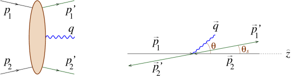
(a)                                             (b)                                          

Figure 2: (a) Diagram representing graviton emission (wavy line) in transplanckian scattering of two sources (straight lines). (b) kinematics in the spatial momentum space.

Consider the basic emission process $p_{1}+p_{2}\to p^{\prime}_{1}+p^{\prime}_{2}+q$ at tree level (fig. 2) of a graviton of momentum $q^{\mu}:{\boldsymbol{q}}=\hbar\omega{\boldsymbol{\theta}}$ and helicity $\lambda$, assuming a relatively soft emission energy $\hbar\omega\ll E$. Note that this restriction still allows for a huge graviton phase space, corresponding to classical frequencies potentially much larger than the characteristic scale $R^{-1}$, due to the large gravitational charge $\alpha_{G}\equiv Gs/\hbar\gg 1$.

We denote with ${\boldsymbol{q}}_{s}$ the single-hit transverse momentum exchanged between particles 1 and 2, and with ${\boldsymbol{\theta}}_{s}=|{\boldsymbol{\theta}}_{s}|(\cos\phi_{s},\sin\phi_{s})={\boldsymbol{q}}_{s}/E$ the corresponding 2D scattering angle (including azimuth). For not too large emission angles $|{\boldsymbol{\theta}}|\ll(E/\hbar\omega)|{\boldsymbol{\theta}}_{s}|$, corresponding to $|{\boldsymbol{q}}|\ll|{\boldsymbol{q}}_{s}|$, Weinberg’s theorem expresses the emission amplitude as the product of the elastic amplitude ${M_{1}}$ and of the external-line insertion factor $J_{W}^{(\lambda)}\equiv J_{W}^{\mu\nu}\epsilon^{(\lambda)*}_{\mu\nu}$, where $\epsilon^{(\lambda)}_{\mu\nu}$ is the polarization tensor of the emitted graviton (see [19] for details) and $J_{W}^{\mu\nu}$ is the Weinberg current [28] [$\eta_{i}=+1(-1)$ for incoming (outgoing) lines]

$$J_{W}^{\mu\nu}=\kappa\sum_{i}\eta_{i}\frac{p_{i}^{\mu}p_{i}^{\nu}}{p_{i}\cdot q}=\kappa\left(\frac{p_{1}^{\mu}p_{1}^{\nu}}{p_{1}\cdot q}-\frac{p^{\prime}_{1}{}^{\mu}p^{\prime}_{1}{}^{\nu}}{p^{\prime}_{1}\cdot q}+\frac{p_{2}^{\mu}p_{2}^{\nu}}{p_{2}\cdot q}-\frac{p^{\prime}_{2}{}^{\mu}p^{\prime}_{2}{}^{\nu}}{p^{\prime}_{2}\cdot q}\right)\;.$$ (2.7)

By referring, for definiteness, to the forward hemisphere and restricting ourselves to the forward region $|{\boldsymbol{\theta}}|,|{\boldsymbol{\theta}}_{s}|\ll 1$ one obtains the following explicit result [19] in the c.m. frame with ${\boldsymbol{p}}_{1}=0$:

$$J_{W}^{(\lambda)}(q^{3}>0;{\boldsymbol{\theta}},{\boldsymbol{\theta}}_{s})=\kappa\frac{E}{\hbar\omega}\;\left(\mathrm{e}^{\mathrm{i}\lambda(\phi_{\boldsymbol{\theta}}-\phi_{{\boldsymbol{\theta}}-{\boldsymbol{\theta}}_{s}})}-1\right)\;,$$ (2.8)

leading to a factorized soft emission amplitude

$$M_{\mathrm{soft}}({\boldsymbol{\theta}}_{s},E,{\boldsymbol{\theta}},\omega)=M_{{\mathrm{el}}}(E,{\boldsymbol{Q}})J_{W}^{(\lambda)}\Big{(}\frac{E}{\hbar\omega},{\boldsymbol{\theta}},{\boldsymbol{\theta}}_{s}\Big{)}=\kappa^{3}s^{2}\frac{1}{E\hbar\omega{\boldsymbol{\theta}}_{s}^{2}}\left(\mathrm{e}^{\mathrm{i}\lambda(\phi_{\boldsymbol{\theta}}-\phi_{{\boldsymbol{\theta}}-{\boldsymbol{\theta}}_{s}})}-1\right)\;,$$ (2.9)

The simple expression (2.8) shows a $1/\omega$ dependence, but no singularities at either ${\boldsymbol{\theta}}=0$ or ${\boldsymbol{\theta}}={\boldsymbol{\theta}}_{s}$ as we might have expected from the $p_{i}\cdot q$ denominators occurring in (2.7). This is due to the helicity conservation zeros in the physical projections of the tensor numerators in (2.7).

The soft amplitude in impact parameter space is readily obtained by Fourier transforming with respect to ${\boldsymbol{Q}}={\boldsymbol{q}}_{s}=E{\boldsymbol{\theta}}_{s}$ and reads

$${\cal M}_{\mathrm{soft}}^{(\lambda)}({\boldsymbol{b}},E,{\boldsymbol{\theta}},\omega) \equiv\frac{1}{(2\pi)^{3/2}}\frac{1}{4s}\int\frac{\mathrm{d}^{2}{\boldsymbol{q}}_{s}}{(2\pi)^{2}}\;\mathrm{e}^{\mathrm{i}{\boldsymbol{q}}_{s}\cdot{\boldsymbol{b}}}M_{\mathrm{soft}}({\boldsymbol{q}}_{s})$$

$$=\sqrt{\alpha_{G}}\frac{R}{\pi}\int\frac{\mathrm{d}^{2}{\boldsymbol{\theta}}_{s}}{2\pi{\boldsymbol{\theta}}_{s}^{2}}\mathrm{e}^{\mathrm{i}\frac{E}{\hbar}{\boldsymbol{b}}\cdot{\boldsymbol{\theta}}_{s}}\frac{E}{\hbar\omega}\frac{1}{2}\left(\mathrm{e}^{\mathrm{i}\lambda(\phi_{{\boldsymbol{\theta}}}-\phi_{{\boldsymbol{\theta}}-{\boldsymbol{\theta}}_{s}})}-1\right)$$ (2.10)

$$=\sqrt{\alpha_{G}}\frac{R}{\pi}\mathrm{e}^{\mathrm{i}\lambda\phi_{{\boldsymbol{\theta}}}}\int\frac{\mathrm{d}^{2}{\boldsymbol{z}}}{2\pi|z|^{2}\mathrm{e}^{\mathrm{i}\lambda\phi_{z}}}\mathrm{e}^{\mathrm{i}b\omega{\boldsymbol{z}}\cdot{\boldsymbol{\theta}}}\frac{E}{\hbar\omega}\log\left|\hat{{\boldsymbol{b}}}-\frac{\hbar\omega}{E}{\boldsymbol{z}}\right|\;,$$

where in the last line we have used an integral representation which will be very useful in the sequel.

For large emission angles $|{\boldsymbol{\theta}}|\gtrsim(E/\hbar\omega)|{\boldsymbol{\theta}}_{s}|$ such that $|{\boldsymbol{q}}|\gtrsim|{\boldsymbol{q}}_{s}|$, graviton emission from internal insertions are no longer negligible, and Weinberg’s formula cannot be applied. However, this region of phase space is a subset of the so called Regge region, characterized by emission angles $|{\boldsymbol{\theta}}|\gg|{\boldsymbol{\theta}}_{s}|$. In the Regge limit, the emission amplitude has a different factorized structure and a different emission current: the Lipatov’s current $J_{L}^{\mu\nu}$ [29]. Furthermore, one has to distinguish two transferred momenta ${\boldsymbol{q}}_{1(2)}\equiv{\boldsymbol{p}}_{1(2)}-{\boldsymbol{p}}_{1(2)}^{\prime}$ such that ${\boldsymbol{q}}={\boldsymbol{q}}_{1}+{\boldsymbol{q}}_{2}$. In the c.m. frame with zero incidence angle (${\boldsymbol{p}}_{1}=E{\boldsymbol{\Theta}}_{i}=0$) and in the forward region $|{\boldsymbol{\theta}}|,|{\boldsymbol{\theta}}_{s}|\ll 1$ (where we identify ${\boldsymbol{q}}_{s}={\boldsymbol{q}}_{2}$), the helicity amplitude takes the form [19]

$$M_{\mathrm{Regge}}^{(\lambda)}({\boldsymbol{\theta}}_{s},E,{\boldsymbol{\theta}},\omega) =\frac{\kappa^{2}s^{2}}{|{\boldsymbol{q}}_{1}|^{2}|{\boldsymbol{q}}_{2}|^{2}}J_{L}^{\mu\nu}\epsilon_{\mu\nu}^{(\lambda)*}=\kappa^{3}s^{2}\frac{1-\mathrm{e}^{\mathrm{i}\lambda(\phi_{{\boldsymbol{q}}_{2}}-\phi_{{\boldsymbol{q}}-{\boldsymbol{q}}_{2}})}}{{\boldsymbol{q}}^{2}}\;,$$ (2.11)

$${\cal M}_{\mathrm{Regge}}^{(\lambda)}({\boldsymbol{b}},E,{\boldsymbol{\theta}},\omega) =\sqrt{\alpha_{G}}\frac{R}{\pi}\mathrm{e}^{\mathrm{i}\lambda\phi_{{\boldsymbol{\theta}}}}\int\frac{\mathrm{d}^{2}{\boldsymbol{z}}}{2\pi|z|^{2}\mathrm{e}^{\mathrm{i}\lambda\phi_{z}}}\mathrm{e}^{\mathrm{i}b\omega{\boldsymbol{z}}\cdot{\boldsymbol{\theta}}}\left(-\hat{{\boldsymbol{b}}}\cdot{\boldsymbol{z}}-\log|\hat{{\boldsymbol{b}}}-{\boldsymbol{z}}|\right)\;.$$ (2.12)

It is not difficult to verify that the soft and Regge amplitudes (2.9), (2.11) agree in the overlapping region of validity $|{\boldsymbol{\theta}}_{s}|\ll{\boldsymbol{\theta}}\ll(E/\hbar\omega)|{\boldsymbol{\theta}}_{s}|$. By exploiting the above expressions, we obtained a unifying amplitude that accurately describes both regimes and that can be written in terms of the soft amplitude only:

$$\frac{{\cal M}_{\mathrm{matched}}^{(\lambda)}}{\sqrt{\alpha_{G}}\frac{R}{\pi}\mathrm{e}^{\mathrm{i}\lambda\phi_{{\boldsymbol{\theta}}}}} =\int\frac{\mathrm{d}^{2}{\boldsymbol{z}}}{2\pi|z|^{2}\mathrm{e}^{\mathrm{i}\lambda\phi_{z}}}\mathrm{e}^{\mathrm{i}b\omega{\boldsymbol{z}}\cdot{\boldsymbol{\theta}}}\left(\frac{E}{\hbar\omega}\log\left|\hat{{\boldsymbol{b}}}-\frac{\hbar\omega}{E}{\boldsymbol{z}}\right|-\log\left|\hat{{\boldsymbol{b}}}-{\boldsymbol{z}}\right|\right) =\mathrm{soft}\big{|}_{E}-\mathrm{soft}\big{|}_{\hbar\omega}$$ (2.13)

The result (2.13) is expressed in terms of the ($\omega$-dependent) “soft” field

$$h_{s}^{(\lambda)}(\omega,z)\equiv\frac{1}{\pi^{2}|z|^{2}\mathrm{e}^{\mathrm{i}\lambda\phi_{z}}}\left(\frac{E}{\hbar\omega}\log\left|\hat{{\boldsymbol{b}}}-\frac{\hbar\omega}{E}{\boldsymbol{z}}\right|-\log\left|\hat{{\boldsymbol{b}}}-{\boldsymbol{z}}\right|\right)\equiv-\frac{\Phi(\omega,{\boldsymbol{z}})}{\pi^{2}|z|^{2}\mathrm{e}^{\mathrm{i}\lambda\phi_{z}}}$$ (2.14)

in which the function $\Phi$ turns out to be useful for the treatment of rescattering too (sec. 2.3). Furthermore, for relatively large angles ($|{\boldsymbol{\theta}}|\gg\theta_{m}\equiv\hbar/(Eb)$), eq. (2.13) involves values of $\hbar\omega|z|/E\lesssim\theta_{m}/|{\boldsymbol{\theta}}|$ which are uniformly small, and the expressions (2.14) can be replaced by their $\omega\to 0$ limits

$$h_{s}^{(\lambda)}(z)=-\frac{\Phi_{\mathrm{cl}}({\boldsymbol{z}})}{\pi^{2}|z|^{2}\mathrm{e}^{\mathrm{i}\lambda\phi_{z}}}\;,\qquad\Phi_{\mathrm{cl}}({\boldsymbol{z}})\equiv\lim_{\omega\to 0}\Phi=\hat{{\boldsymbol{b}}}\cdot{\boldsymbol{z}}+\log\left|\hat{{\boldsymbol{b}}}-{\boldsymbol{z}}\right|\;,$$ (2.15)

which is the field occurring in the Regge amplitude (2.12); the modulating function $\Phi_{\mathrm{cl}}$ appears also in the classical analysis of radiation [13].

The last aspect we have to take into account in order to determine the general $2\to 3$ high-energy emission amplitude at lowest order, is to consider the case of incoming particles with generic direction of momenta. Since we always work in the c.m. frame, we parametrize $\vec{p}_{1}=E({\boldsymbol{\Theta}}_{i},\sqrt{1-{\boldsymbol{\Theta}}_{i}^{2}})$, where ${\boldsymbol{\Theta}}_{i}=|{\boldsymbol{\Theta}}_{i}|(\cos\phi_{i},\sin\phi_{i})$ is a 2D vector that describes both polar and azimuthal angles of the incoming particles. In [19] we proved the transformation formula for the generic helicity amplitude

$${\cal M}^{(\lambda)}({\boldsymbol{b}},E,{\boldsymbol{\theta}},\omega;{\boldsymbol{\Theta}}_{i})=\mathrm{e}^{\mathrm{i}\lambda(\phi_{\boldsymbol{\theta}}-\phi_{{\boldsymbol{\theta}}-{\boldsymbol{\Theta}}_{i}})}{\cal M}^{(\lambda)}({\boldsymbol{b}},E,{\boldsymbol{\theta}}-{\boldsymbol{\Theta}}_{i},\omega;\boldsymbol{0})\;.$$ (2.16)

By applying eq. (2.16) to the matched amplitude (2.13), one immediately finds

$${\cal M}_{\mathrm{matched}}({\boldsymbol{b}},E,{\boldsymbol{\theta}},\omega;{\boldsymbol{\Theta}}_{i})=\sqrt{\alpha_{G}}\frac{R}{2}\mathrm{e}^{\mathrm{i}\lambda\phi_{{\boldsymbol{\theta}}}}\int\mathrm{d}^{2}{\boldsymbol{z}}\;\mathrm{e}^{\mathrm{i}b\omega{\boldsymbol{z}}\cdot({\boldsymbol{\theta}}-{\boldsymbol{\Theta}}_{i})}h_{s}^{(\lambda)}(\omega,z)$$ (2.17)

and the whole ${\boldsymbol{\Theta}}_{i}$ dependence amounts to a shift in the exponential factor.

2.3 Eikonal emission and rescattering

The physics of transplanckian scattering is captured, at leading level, by the resummation of eikonal diagrams, as illustrated in sec. 2.1. In order to compute the associated graviton radiation, it is therefore mandatory to consider graviton emission from all ladder diagrams, as depicted in fig. 3.

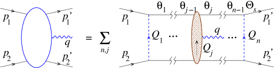
Figure 3: Graviton emission from the eikonal ladder. The $n$-rung diagram with the emission from the $j$-th exchange is denoted by ${\cal M}^{[n,j]}$ in the text.

As we shew in ref. [19], the crucial fact is that all internal lines insertions — for fast particles and exchanged particles alike — can be accounted for by calculating $n$ diagrams for the eikonal contribution with $n$ exchanged gravitons, where the matched amplitude (2.17) is inserted in turn in correspondence to the $j$-th exchanged graviton (fig. 3), adjusting for the local incidence angle ${\boldsymbol{\Theta}}_{i}={\boldsymbol{\theta}}_{j-1}$.

The ladder-like structure of such amplitude in momentum space is a convolution in the ${\boldsymbol{Q}}_{j}$ variables, with ${\boldsymbol{Q}}_{1}+\cdots+{\boldsymbol{Q}}_{n}={\boldsymbol{Q}}$. Thus in impact parameter space the amplitude is obtained as a product of $j-1$ elastic amplitudes, the emission amplitude from the $j$-th leg, and $n-j$ elastic amplitudes, whose upper particle, by energy conservation, has reduced energy $E\to E-\hbar\omega$.

Let us express the elastic amplitude in terms of the dimensionless function $\Delta({\boldsymbol{b}})$ such that

$${\cal M}_{\mathrm{el}}({\boldsymbol{b}},E)=2\delta({\boldsymbol{b}},s=4EE^{\prime})\equiv 2R\frac{E}{\hbar}\Delta({\boldsymbol{b}})\;,\qquad\Delta_{0}({\boldsymbol{b}})=\log\left(\frac{L}{b}\right)\;,$$ (2.18)

so as to explicitly show the linear proportionality of the amplitude on the upper (jet 1) particle energy $E$ (which varies after graviton emission). The energy $E^{\prime}$ of the lower particle (jet 2) stays unchanged and its dependence has been absorbed in the constant $R=4GE^{\prime}$.

The $n$-rung amplitude for emission of a graviton with momentum $q$ from the $j$-th exchange of the ladder can then be expressed by the $z$-representation

$$\mathrm{i}{\cal M}^{[n,j]}_{\lambda}({\boldsymbol{b}},\omega,{\boldsymbol{\theta}}) =\mathrm{e}^{\mathrm{i}\lambda\phi_{\boldsymbol{\theta}}}\sqrt{\alpha_{G}}\frac{R}{2}\times$$

$$\quad\frac{\mathrm{i}^{n}}{n!}\int\mathrm{d}^{2}{\boldsymbol{z}}\;\mathrm{e}^{\mathrm{i}b\omega{\boldsymbol{\theta}}\cdot{\boldsymbol{z}}}\left[{\cal M}_{\mathrm{el}}({\boldsymbol{b}}-\frac{\hbar\omega}{E}b{\boldsymbol{z}},E)\right]^{j-1}h_{s}^{(\lambda)}(\omega,z)\left[{\cal M}_{\mathrm{el}}({\boldsymbol{b}},E-\hbar\omega)\right]^{n-j}\;.$$ (2.19)

Note the effect of the incidence angle ${\boldsymbol{\Theta}}_{i}={\boldsymbol{\theta}}_{j-1}=({\boldsymbol{Q}}_{1}+\cdots+{\boldsymbol{Q}}_{j-1})/E$ in the exponent of eq. (2.17) which, after Fourier transform, has shifted the impact parameters of the first elastic amplitudes by the amount $-\frac{\hbar\omega}{E}b{\boldsymbol{z}}$. In addition, as already mentioned, the energy of the upper particle after the emission, has the reduced value $E-\hbar\omega$, and this modifies the second argument of the elastic amplitudes after the emission.

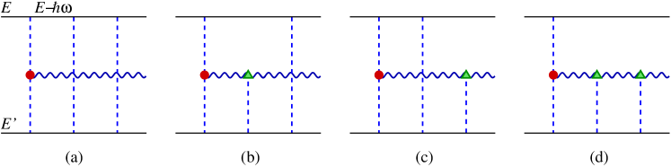
Figure 4: Rescattering contributions (b,c,d) to eikonal graviton emission (a).

Before summing all ladder diagrams, we take into account the rescattering of the emitted graviton with the external particles $p_{j}:j=1,2$. This interaction is proportional to $G(p_{j}+q)^{2}$, and is dominated by the exchange of gravitons between $q$ and $p_{2}$, since $(p_{1}+q)^{2}\sim\hbar\omega E|{\boldsymbol{\theta}}-{\boldsymbol{\theta}}_{j}|^{2}\ll(p_{2}+q)^{2}\sim\hbar\omega E$ in the region of forward emission that we are considering. In practice, we add to the rightmost factor $\left[{\cal M}_{\mathrm{el}}({\boldsymbol{b}},E-\hbar\omega)\right]^{n-j}$ in eq. (2.19) (represented by the ladder of fig. 4.a) the contributions coming from rescattering diagrams where graviton exchanges between $p_{1}$ and $p_{2}$ are replaced by exchanges between $q$ and $p_{2}$ in all possible ways (fig. 4.b,c,d). Since the ordering among eikonal exchanges and rescattering factors is irrelevant, the inclusion of such additional contributions amounts to the replacement ($N=n-j$)

$$\left[{\cal M}_{\mathrm{el}}({\boldsymbol{b}},E-\hbar\omega)\right]^{N} \to\sum_{r=0}^{N}{{N}\choose{r}}\left[{\cal M}_{\mathrm{el}}({\boldsymbol{b}},E-\hbar\omega)\right]^{N-r}\left[{\cal M}_{\mathrm{el}}({\boldsymbol{b}}-{\boldsymbol{x}},\hbar\omega)\right]^{r}$$

$$=\left[{\cal M}_{\mathrm{el}}({\boldsymbol{b}},E-\hbar\omega)+{\cal M}_{\mathrm{el}}({\boldsymbol{b}}-{\boldsymbol{x}},\hbar\omega)\right]^{N}$$

$$=\{2R[(E/\hbar-\omega)\Delta({\boldsymbol{b}})+\omega\Delta({\boldsymbol{b}}-{\boldsymbol{x}})]\}^{N}$$ (2.20)

where we took into account that in diagrams with $N$ exchanged gravitons there are ${{N}\choose{r}}$ distinct diagrams with $r$ rescattering gravitons, and that in each rescattering factor the energy of the upper particle (i.e., the emitted graviton) is $\hbar\omega$. Furthermore, we took into account that the transverse position of the emitted graviton with respect to the lower particle (i.e., $p_{2}$) is ${\boldsymbol{b}}-{\boldsymbol{x}}$, where ${\boldsymbol{x}}=b{\boldsymbol{z}}$ is the variable conjugated to ${\boldsymbol{q}}=\omega{\boldsymbol{\theta}}$ [cf. eq. (2.19)], hence to be interpreted as the transverse position of the emitted graviton with respect to $p_{1}$.

Substituting the expression of eq. (2.20) into eq. (2.19), we can perform the sum over $n$ and $j$ of all diagrams with the aid of the formula

$$\sum_{n=1}^{\infty}\frac{1}{n!}\sum_{j=1}^{n}A^{j-1}B^{n-j}=\sum_{n=0}^{\infty}\frac{1}{n!}\frac{A^{n}-B^{n}}{A-B}=\frac{\mathrm{e}^{A}-\mathrm{e}^{B}}{A-B}\;.$$ (2.21)

It is also convenient to express the $A$ and $B$ quantities as the elastic amplitude (2.18) plus a quantum correction $\Phi_{A,B}$ as follows:

$$A \equiv\mathrm{i}{\cal M}_{\mathrm{el}}({\boldsymbol{b}}-\frac{\hbar\omega}{E}{\boldsymbol{x}},E)=2\mathrm{i}{\alpha_{G}}\left[\Delta({\boldsymbol{b}})+\frac{\hbar\omega}{E}\Phi_{A}({\boldsymbol{x}})\right]$$

$$B \equiv\mathrm{i}\left[{\cal M}_{\mathrm{el}}({\boldsymbol{b}},E-\hbar\omega)+{\cal M}_{\mathrm{el}}({\boldsymbol{b}}-{\boldsymbol{x}},\hbar\omega)\right]=2\mathrm{i}{\alpha_{G}}\left[\Delta({\boldsymbol{b}})+\frac{\hbar\omega}{E}\Phi_{B}({\boldsymbol{x}})\right]$$

$$\Phi_{A}({\boldsymbol{x}}) \equiv\frac{E}{\hbar\omega}[\Delta({\boldsymbol{b}}-\frac{\hbar\omega}{E}{\boldsymbol{x}})-\Delta({\boldsymbol{b}})]=-\Delta^{\prime}({\boldsymbol{b}})\cdot{\boldsymbol{x}}+\mathcal{O}\left(\frac{\hbar\omega}{E}\right)$$ (2.22a)

$$\Phi_{B}({\boldsymbol{x}}) \equiv\Delta({\boldsymbol{b}}-{\boldsymbol{x}})-\Delta({\boldsymbol{b}})]=\Phi_{A}({\boldsymbol{x}})|_{E\to\hbar\omega}\;.$$ (2.22b)

We note that the denominator in eq. (2.21) is proportional to the $\Phi$ function defined in eq. (2.14)

$$A-B=2\mathrm{i}{\alpha_{G}}\frac{\hbar\omega}{E}\left[\Phi_{A}-\Phi_{B}\right]=2\mathrm{i}\omega R\Phi$$ (2.23)

and is therefore intimately related to the soft field $h_{s}$.

From the technical point of view, such relation provides the cancellation between $h_{s}$ in eq. (2.19) and the mentioned denominator $A-B$ of (2.21), to yield finally the one-graviton emission amplitude

$$\mathrm{i}{\cal M}_{\lambda}({\boldsymbol{b}};\omega,{\boldsymbol{\theta}}) =\mathrm{e}^{\mathrm{i}{\alpha_{G}}2\Delta(b)}\mathfrak{M}_{\lambda}({\boldsymbol{b}};\omega,{\boldsymbol{\theta}})$$

$$\frac{\mathfrak{M}_{\lambda}({\boldsymbol{b}};\omega,{\boldsymbol{\theta}})}{\mathrm{e}^{\mathrm{i}\lambda\phi_{\boldsymbol{\theta}}}} \equiv\sqrt{\alpha_{G}}\frac{R}{\pi}\int\frac{\mathrm{d}^{2}{\boldsymbol{z}}}{2\pi|z|^{2}\mathrm{e}^{\mathrm{i}\lambda\phi_{z}}}\;\mathrm{e}^{\mathrm{i}b\omega{\boldsymbol{\theta}}\cdot{\boldsymbol{z}}}\mathrm{e}^{2\mathrm{i}\omega R\Phi_{A}}\frac{\mathrm{e}^{-2\mathrm{i}\omega R\Phi}-1}{2\mathrm{i}\omega R}\;,$$ (2.24)

which reduces to the classical expression (4.11) of [13] in the limit $\hbar\omega/E\to 0$, $\lambda=-2$ and $\Delta=\Delta_{0}$, since $\Phi\to\Phi_{\mathrm{cl}}$ [cf. eq. (2.15)] and $2R\Phi_{A}\to 2R\hat{{\boldsymbol{b}}}\cdot{\boldsymbol{z}}=-b{\boldsymbol{\Theta}}_{s}\cdot{\boldsymbol{z}}$.

From the conceptual point of view, the identity (2.23) is surprising because it relates the exponents (which describe elastic plus rescattering exchanges) to the soft field $\sim\Phi$ (which describes graviton emission). The explanation lies in the derivation [19] of the soft-based representation (2.13) whose form

$${\cal M}_{\mathrm{matched}}=\left.\mathrm{soft}\right|_{E}-\left.\mathrm{soft}\right|_{\hbar\omega}\simeq\left.\mathrm{Regge}\right|_{E}$$ (2.25)

has the alternative interpretations of external plus internal insertions in the soft-emission language and of elastic plus rescattering ones in the Regge language.

We shall base on that representation the generalized emission amplitude including subleading corrections, that will be investigated in sec. 3 [eqs. (3.26) and (3.29)].

2.4 Multi-graviton emission and linear coherent state

In order to compute the multi-graviton emission amplitude from eikonal ladder diagrams, let us start from the two-graviton emission process. We exploit again the ${\boldsymbol{b}}$-space factorization formula of Regge-amplitudes. Referring to fig. 5, if graviton 1 is emitted first from the $j_{1}$-th rung and then graviton 2 from the $j_{2}$-th rung ($j_{1}<j_{2}$) of an $n$-rung ladder, the corresponding amplitude reads

$$\mathrm{i}{\cal M}^{[n,(j_{1}<j_{2})]}(1,2) =\frac{\mathrm{i}^{n}}{2!n!}\mathrm{e}^{\mathrm{i}(\lambda_{1}\phi_{{\boldsymbol{\theta}}_{1}}+\lambda_{2}\phi_{{\boldsymbol{\theta}}_{2}})}\left(\sqrt{{\alpha_{G}}}\frac{R}{2}\right)^{2}\int\mathrm{d}^{2}{\boldsymbol{x}}_{1}\mathrm{d}^{2}{\boldsymbol{x}}_{2}\;\mathrm{e}^{\mathrm{i}(\omega_{1}{\boldsymbol{\theta}}_{1}\cdot{\boldsymbol{x}}_{1}+\omega_{2}{\boldsymbol{\theta}}_{2}\cdot{\boldsymbol{x}}_{2})}$$

$$\quad\times A^{j_{1}-1}h_{s}({\boldsymbol{b}},{\boldsymbol{x}}_{1},\omega_{1})B^{j_{2}-j_{1}-1}h_{s}({\boldsymbol{b}},{\boldsymbol{x}}_{2},\omega_{2})C^{n-j_{2}}$$ (2.26)

where, as before, the fields $h_{s}$ describe real graviton production, while graviton exchanges and rescattering are encoded by the quantities

$$A =\mathrm{i}{\cal M}_{\mathrm{el}}({\boldsymbol{b}}-\frac{\hbar\omega_{1}{\boldsymbol{x}}_{1}+\hbar\omega_{2}{\boldsymbol{x}}_{2}}{E},E)$$

$$B =\mathrm{i}{\cal M}_{\mathrm{el}}({\boldsymbol{b}}-\frac{\hbar\omega_{2}}{E}{\boldsymbol{x}}_{2},E-\hbar\omega_{1})+\mathrm{i}{\cal M}_{\mathrm{el}}({\boldsymbol{b}}-{\boldsymbol{x}}_{1},\hbar\omega_{1})$$

$$C =\mathrm{i}{\cal M}_{\mathrm{el}}({\boldsymbol{b}},E-\hbar\omega_{1}-\hbar\omega_{2})+\mathrm{i}{\cal M}_{\mathrm{el}}({\boldsymbol{b}}-{\boldsymbol{x}}_{1},\hbar\omega_{1})+\mathrm{i}{\cal M}_{\mathrm{el}}({\boldsymbol{b}}-{\boldsymbol{x}}_{2},\hbar\omega_{2})\;.$$ (2.27)

The quantity $A$ denotes the eikonal exchanges before any graviton emission, and is given by the elastic amplitude ${\cal M}_{\mathrm{el}}$ with a shift in its first argument due to the effect of the incidence-angles ${\boldsymbol{\Theta}}_{j_{1}-1},{\boldsymbol{\Theta}}_{j_{2}-1}$ of both gravitons, an effect that propagates backwards in the ladder, as explained in the previous section.

Figure 5: Double graviton emission from eikonal ladder. $A$ denotes eikonal exchanges before graviton emissions, $B$ eikonal exchanges and rescattering of graviton 1, $C$ includes also rescattering of graviton 2.

The quantity $B$ describes the interactions occurring in the middle of the ladder, i.e., after the emission of graviton 1 and before that of graviton 2. It consists in the sum of two terms: the first one describes the eikonal exchanges between $p_{1}$ and $p_{2}$, and includes both the effect of the incidence angle ${\boldsymbol{\Theta}}_{j_{2}-1}$ (shift in the first argument) and also the reduced gravitational coupling $E\to E-\hbar\omega_{1}$ in the upper vertices due to energy conservation. The second term describes rescattering of graviton 1 with $p_{2}$.

Finally, the first of the three terms building $C$ represents the eikonal exchanges between $p_{1}$ and $p_{2}$ with reduced coupling $E\to E-\hbar(\omega_{1}+\omega_{2})$ in the upper vertices, while the other two terms take into account rescattering corrections of both gravitons.

The sum over all such ladder diagrams amounts to

$$\mathfrak{S}(1,2) \equiv\sum_{n=2}^{\infty}\frac{1}{n!}\sum_{j_{1}=1}^{n-1}\sum_{j_{2}=j_{1}+1}^{n}A^{j_{1}-1}B^{j_{2}-j_{1}-1}C^{n-j_{2}}$$

$$=\frac{\mathrm{e}^{A}}{(A-B)(A-C)}+\frac{\mathrm{e}^{B}}{(B-A)(B-C)}+\frac{\mathrm{e}^{C}}{(C-A)(C-B)}\;.$$ (2.28)

By swapping the graviton indices $1\leftrightarrow 2$ one immediately obtains the symmetric contribution with graviton 2 emitted “before” graviton 1.

Now, the sum of these two contributions doesn’t factorize exactly in two independent factors. It would if $A-B=[B-C]_{1\leftrightarrow 2}$, but this is not the case. However, $A-B=[B-C]_{1\leftrightarrow 2}+\mathcal{O}\left(A\hbar^{2}\omega_{i}^{2}/E^{2}\right)$, therefore factorization can be recovered by neglecting contributions of relative order $\mathcal{O}\left(\hbar^{2}\omega_{i}^{2}/E^{2}\right)$. In fact, thanks to eqs. (2.22), we have

$$A =2\mathrm{i}{\alpha_{G}}\Delta({\boldsymbol{b}}-\frac{\hbar\omega_{1}{\boldsymbol{x}}_{1}+\hbar\omega_{2}{\boldsymbol{x}}_{2}}{E})=2\mathrm{i}{\alpha_{G}}\left[\Delta({\boldsymbol{b}})-\Delta^{\prime}(b)\cdot\frac{\hbar\omega_{1}{\boldsymbol{x}}_{1}+\hbar\omega_{2}{\boldsymbol{x}}_{2}}{E}+\mathcal{O}\left(\frac{\hbar^{2}\omega_{i}^{2}}{E^{2}}\right)\right]$$

$$=2\mathrm{i}\left\{{\alpha_{G}}\Delta({\boldsymbol{b}})+\omega_{1}R\Phi_{A}({\boldsymbol{x}}_{1})+\omega_{2}R\Phi_{A}({\boldsymbol{x}}_{2})+\mathcal{O}\left(G\hbar^{2}\omega_{i}^{2}\right)\right\}$$

$$B =2\mathrm{i}{\alpha_{G}}\left[\left(1-\frac{\hbar\omega_{1}{\boldsymbol{x}}_{1}}{E}\right)\Delta({\boldsymbol{b}}-\frac{\hbar\omega_{2}{\boldsymbol{x}}_{2}}{E})+\frac{\hbar\omega_{1}{\boldsymbol{x}}_{1}}{E}\Delta({\boldsymbol{b}}-{\boldsymbol{x}}_{1})\right]$$

$$=2\mathrm{i}\left\{{\alpha_{G}}\Delta({\boldsymbol{b}})+\omega_{2}R\Phi_{A}({\boldsymbol{x}}_{2})+\omega_{1}R\Phi_{B}({\boldsymbol{x}}_{1})+\mathcal{O}\left(G\hbar^{2}\omega_{i}^{2}\right)\right\}$$

$$C =\mathrm{i}2{\alpha_{G}}\left[\left(1-\frac{\hbar\omega_{1}{\boldsymbol{x}}_{1}}{E}-\frac{\hbar\omega_{2}{\boldsymbol{x}}_{2}}{E}\right)\Delta({\boldsymbol{b}})+\frac{\hbar\omega_{1}{\boldsymbol{x}}_{1}}{E}\Delta({\boldsymbol{b}}-{\boldsymbol{x}}_{1})+\frac{\hbar\omega_{1}{\boldsymbol{x}}_{2}}{E}\Delta({\boldsymbol{b}}-{\boldsymbol{x}}_{2})\right]$$

$$=2\mathrm{i}\left\{{\alpha_{G}}\Delta({\boldsymbol{b}})+\omega_{1}R\Phi_{B}({\boldsymbol{x}}_{1})+\omega_{2}R\Phi_{B}({\boldsymbol{x}}_{2})\right\}$$ (2.29)

By noting that the elastic amplitude $\mathrm{e}^{2\mathrm{i}{\alpha_{G}}\Delta({\boldsymbol{b}})}$ is a common factor in all exponentials, we can approximate the infinite sum (2.28) in the form

$$\mathfrak{S}(1,2)\simeq\mathrm{e}^{2\mathrm{i}{\alpha_{G}}\Delta}\left[\frac{\mathrm{e}^{\varphi_{A1}+\varphi_{A2}}}{\varphi_{1}(\varphi_{1}+\varphi_{2})}-\frac{\mathrm{e}^{\varphi_{B1}+\varphi_{A2}}}{\varphi_{1}\varphi_{2}}+\frac{\mathrm{e}^{\varphi_{B1}+\varphi_{B2}}}{(\varphi_{1}+\varphi_{2})\varphi_{2}}\right]\;,$$ (2.30)

where we used the shortcuts $\varphi_{A1}\equiv 2\mathrm{i}\omega_{1}R\Phi_{A}({\boldsymbol{x}}_{1})$ and analogous ones.

At this point, it is straightforward to check that

$$\mathfrak{S}(1,2)+\mathfrak{S}(2,1)\simeq\mathrm{e}^{2\mathrm{i}{\alpha_{G}}\Delta}\frac{\mathrm{e}^{\varphi_{A1}}(\mathrm{e}^{-\varphi_{1}}-1)}{\varphi_{1}}\frac{\mathrm{e}^{\varphi_{A2}}(\mathrm{e}^{-\varphi_{2}}-1)}{\varphi_{2}}$$ (2.31)

and to obtain the two-graviton emission amplitude in factorized form:

$$\mathrm{i}{\cal M}_{\lambda_{1}\lambda_{2}}({\boldsymbol{b}};\omega_{1},{\boldsymbol{\theta}}_{1};\omega_{2}{\boldsymbol{\theta}}_{2})\simeq\mathrm{e}^{\mathrm{i}{\alpha_{G}}2\Delta(b)}\mathfrak{M}_{\lambda_{1}}({\boldsymbol{b}};\omega_{1},{\boldsymbol{\theta}}_{1})\mathfrak{M}_{\lambda_{2}}({\boldsymbol{b}};\omega_{2},{\boldsymbol{\theta}}_{2})\;.$$ (2.32)

in terms of the one-graviton amplitude and of the elastic $S$-matrix. It is clear from eqs. (2.29) that such approximate relation neglects terms of relative order $\mathcal{O}\left(\hbar^{2}\omega^{2}/E^{2}\right)=\mathcal{O}\left(\omega R/{\alpha_{G}}\right)^{2}$, which are negligible in the regime we are considering, and are subleading not only with respect to terms $\sim{\alpha_{G}}$ (like the eikonal phase $\delta({\boldsymbol{b}})$) but also with respect to the terms $\sim\omega R$.

We expect an analogous factorization formula to hold for the generic $N$-graviton emission amplitude off eikonal ladders (we explicitly checked the 3-graviton case), in the form

$$\mathrm{i}{\cal M}({\boldsymbol{b}};q_{1},\cdots,q_{N})\simeq\mathrm{e}^{\mathrm{i}{\alpha_{G}}2\Delta(b)}\prod_{r=1}^{N}\mathfrak{M}_{\lambda_{r}}({\boldsymbol{b}};\omega_{r},{\boldsymbol{\theta}}_{r})\;.$$ (2.33)

Such an independent emission pattern corresponds to the final state

$$|\text{gravitons; out}\rangle=\sqrt{P_{0}}\exp\left\{\int\frac{\mathrm{d}^{3}q}{\hbar^{3}\sqrt{2\omega}}\;2\mathrm{i}\sum_{\lambda}\mathfrak{M}_{\lambda}({\boldsymbol{b}},\vec{q})a^{\dagger}_{\lambda}(\vec{q})\right\}|0\rangle$$ (2.34)

in the Fock space of gravitons, with $P_{0}=1$, and creation ($a^{\dagger}_{\lambda}(\vec{q})$) and destruction ($a_{\lambda}(\vec{q})$) operators of definite helicity $\lambda$ are normalized to a wave-number $\delta$-function commutator $[a_{\lambda}(\vec{q}),a^{\dagger}_{\lambda^{\prime}}(\vec{q}\,^{\prime})]=\hbar^{3}\delta^{3}(\vec{q}-\vec{q}\,^{\prime})\delta_{\lambda\lambda^{\prime}}$. However, this state takes into account only real emission. Virtual corrections can then be incorporated by exponentiating both creation and destruction operators in a (unitary) coherent state operator acting on the graviton vacuum $|0\rangle$ (the initial state of gravitons). We thus obtain the full $S$-matrix

$$\hat{S}=\mathrm{e}^{2\mathrm{i}\delta}\exp\left\{\int\frac{\mathrm{d}^{3}q}{\hbar^{3}\sqrt{2\omega}}\;2\mathrm{i}\left[\sum_{\lambda}\mathfrak{M}_{\lambda}({\boldsymbol{b}},\vec{q})a^{\dagger}_{\lambda}(\vec{q})+\text{h.c.}\right]\right\}$$ (2.35)

that is unitary, because of the anti-hermitian exponent, when $b>b_{c}$.

By normal ordering eq. (2.35) when acting on the initial state $|0\rangle$, we find that the final state of graviton is still given by eq. (2.34), but with $P_{0}$ given by

$$P_{0}=\exp\left\{-2\int\frac{\mathrm{d}^{3}q}{\hbar^{3}\omega}\;\sum_{\lambda}|\mathfrak{M}_{\lambda}({\boldsymbol{b}},\vec{q})|^{2}\right\}\;,$$ (2.36)

which is just the no-emission probability, coming from the $a,a^{\dagger}$ commutators.

Due to the factorized structure of eq. (2.34), it is straightforward to derive the inclusive distributions of gravitons and even their generating functional

$$\mathcal{G}[z_{\lambda}(\vec{q})]=\exp\left\{2\int_{\Delta\omega}\frac{\mathrm{d}^{3}q}{\hbar^{3}\omega}\;\sum_{\lambda}|\mathfrak{M}_{\boldsymbol{b}}^{(\lambda)}(\vec{q})|^{2}\left[z_{\lambda}(\vec{q})-1\right]\right\}\;.$$ (2.37)

In particular, the polarized energy emission distribution in the solid angle $\Omega$ and its multiplicity density are given by

$$\frac{\mathrm{d}E_{\lambda}^{\mathrm{GW}}}{\mathrm{d}\omega\,\mathrm{d}\Omega}=\hbar\omega\frac{\mathrm{d}\mathcal{N}_{\lambda}}{\mathrm{d}\omega\,\mathrm{d}\Omega}=2\omega^{2}\hbar|\mathfrak{M}_{\lambda}({\boldsymbol{b}},\vec{q})|^{2}\;,\quad\frac{\mathrm{d}\mathcal{N}}{\mathrm{d}\omega}=p(\omega)=\frac{1}{\hbar\omega}\frac{\mathrm{d}E^{\mathrm{GW}}}{\mathrm{d}\omega}$$ (2.38)

Both quantities will be discussed in the next section.

2.5 Large $\boldsymbol{\omega R}$ emission amplitude

In this section we analyse the graviton emission amplitude (2.24) and its spectrum (2.38) generated by a small-angle ($\Theta_{s}\ll 1$) scattering in the frequency region $\omega\gtrsim R^{-1}$ and in the classical limit $\hbar\omega\ll E$.

We recall that the frequency spectrum integrated in the solid angle was already studied in ref. [19] for large impact parameters $b\gg R$, i.e., for small deflection angles $\Theta_{s}\ll 1$, both with and without rescattering corrections. We briefly report the main results:

• For $\omega R\lesssim\Theta_{s}$ the spectrum is flat and agrees with the zero-frequency-limit.

• For $\Theta_{s}\lesssim\omega R\lesssim 1$ the spectrum shows a slow (logarithmic) decrease with frequency. The behaviour in these two regions is rather insensitive to the inclusion of rescattering, and can be summarized by

  $$\frac{\mathrm{d}E^{\mathrm{GW}}}{\mathrm{d}\omega}\simeq Gs\Theta_{E}^{2}\left[\frac{2}{\pi}\log\min\left(\frac{1}{\Theta_{s}},\frac{1}{\omega R}\right)+\text{const}\right]\qquad(\omega R\lesssim 1)\;;$$ (2.39)

• For $\omega R\gtrsim 1$ the amplitude (2.24) is dominated by small-$z$ values, and the ${\boldsymbol{z}}$-integration can be safely extended to arbitrary large values without introducing spurious effects. The frequency distribution of radiated energy can then be well approximated by computing the square modulus of the amplitude (2.24) by means of the Parseval identity, yielding

  $$\frac{\mathrm{d}E^{\mathrm{GW}}}{\mathrm{d}\omega}=2Gs\frac{\Theta_{E}^{2}}{\pi^{2}}\int\frac{\mathrm{d}^{2}{\boldsymbol{z}}}{|z|^{4}}\;\left(\frac{\sin\omega R\Phi({\boldsymbol{z}})}{\omega R}\right)^{2}\qquad(\omega R\gtrsim 1)\;,$$ (2.40)

  whose asymptotic behaviour provides a spectrum decreasing like $1/\omega$; more precisely

  $$\frac{\mathrm{d}E^{\mathrm{GW}}}{\mathrm{d}\omega}\simeq Gs\Theta_{E}^{2}\frac{1}{\pi\omega R}\qquad(\omega R\gg 1)\;.$$ (2.41)

  In this region the inclusion of rescattering has the effect of lowering the spectrum by about 20%. In any case, the total radiated-energy fraction up to the kinematical bound $\omega_{M}=E/\hbar$ becomes

  $$\frac{E^{\mathrm{GW}}}{\sqrt{s}}=\frac{\Theta_{E}^{2}}{2\pi}\log{\alpha_{G}}$$ (2.42)

  and may exceed unity, thus signalling the need for energy-conservation corrections at sizeable angles (cf. sec. 4).

In fig. 6 we show the energy spectrum (divided by $Gs\Theta_{E}^{2}$) for various values of $\Theta_{s}$. It is apparent that, for $\omega R\gg 1$, its shape is almost independent of $\Theta_{s}$. As we will show in sec. 3, there will be qualitative differences when approaching the strong-coupling region $\Theta_{s}\sim 1$ where subleading contributions become important.

Figure 6: Frequency spectrum of gravitational radiation for various values of $\Theta_{s}$. For each $\Theta_{s}>0$ the ZFL value $\frac{2}{\pi}\log(1.65/\Theta_{s})$ is obtained (dashed lines).

On the contrary, the angular distribution of graviton radiation studied in ref. [19] didn’t take into account rescattering contributions. The latter are actually irrelevant for $\omega R\ll 1$, but change drastically the angular pattern for $\omega R\gg 1$. In fact, the graviton exchanges between the outgoing graviton $q$ and $p_{2}$ (see fig. 4) have the main effect of deflecting the direction of $q$, just like the eikonal exchanges between $p_{1}$ and $p_{2}$ are responsible of the deflection of $p_{1}$ (and $p_{2}$). It turns out that the graviton radiation is collimated around the direction ${\boldsymbol{\Theta}}_{s}$ of the outgoing particle(s).

Quantitatively, the resummed emission amplitude (2.24) in the classical limit $\hbar\omega\ll E$ and, say, for helicity $\lambda=-2$, reads

$$\mathfrak{M}_{\mathrm{cl}}({\boldsymbol{b}},{\boldsymbol{\theta}})=\sqrt{{\alpha_{G}}}\frac{R}{\pi}\mathrm{e}^{-2\mathrm{i}\phi_{\boldsymbol{\theta}}}\int\frac{\mathrm{d}^{2}{\boldsymbol{z}}}{2\pi{z^{*}}^{2}}\;\frac{\mathrm{e}^{\mathrm{i}\omega b{\boldsymbol{z}}\cdot({\boldsymbol{\theta}}-{\boldsymbol{\Theta}}_{s})}}{2\mathrm{i}\omega R}\left(\mathrm{e}^{-2\mathrm{i}\omega R\Phi_{\mathrm{cl}}({\boldsymbol{z}})}-1\right)\;,$$ (2.43)

where ${\boldsymbol{\Theta}}_{s}$ is the fast-particle scattering angle and $\Phi_{\mathrm{cl}}$ was defined in eq. (2.15). We are interested in evaluating such amplitude at large $\omega R$. Since in the second exponential the function

$$\Phi_{\mathrm{cl}}({\boldsymbol{z}})\equiv\hat{{\boldsymbol{b}}}\cdot{\boldsymbol{z}}+\log\left|\hat{{\boldsymbol{b}}}-{\boldsymbol{z}}\right|=\frac{1}{2}(z_{2}^{2}-z_{1}^{2})+\mathcal{O}\left(|z|^{3}\right)$$ (2.44)

vanishes (quadratically) at the origin, we expect that for $\omega R\gg 1$ the dominant contributions to the amplitude come from the small-$z$ integration region. By substituting the second-order expansion (2.44) into eq. (2.43) and by rescaling the integration variable $\sqrt{\omega R}\,z\equiv Z\equiv x+\mathrm{i}y$, we obtain

$$\frac{2\pi\omega\mathfrak{M}}{\sqrt{{\alpha_{G}}}\,\mathrm{e}^{-2\mathrm{i}\phi_{\boldsymbol{\theta}}}}\equiv I({\boldsymbol{A}})=\int\frac{\mathrm{d}^{2}Z}{2\pi Z^{*}{}^{2}}\;\mathrm{e}^{\mathrm{i}2{\boldsymbol{A}}\cdot{\boldsymbol{Z}}}\left[\mathrm{e}^{\mathrm{i}(x^{2}-y^{2})}-1\right]\frac{1}{\mathrm{i}}\;.$$ (2.45)

which is a function of the 2-dimensional variable

$${\boldsymbol{A}}\equiv|{\boldsymbol{A}}|(\cos\phi_{A},\sin\phi_{A})\equiv\sqrt{\omega R}\,\frac{{\boldsymbol{\theta}}-{\boldsymbol{\Theta}}_{s}}{|{\boldsymbol{\Theta}}_{s}|}\;,\qquad A\equiv|{\boldsymbol{A}}|\mathrm{e}^{\mathrm{i}\phi_{A}}\in\mathbb{C}\;.$$ (2.46)

Were it not for the factor $Z^{*}{}^{2}$ in the denominator, the r.h.s. of eq. (2.45) would have the structure of a gaussian integral in 2 dimensions. It is possible however to provide a simple one-dimensional integral representation for the function $I({\boldsymbol{A}})$ in eq. (2.45) (see app. B):

$$I({\boldsymbol{A}})=-\frac{A}{2A^{*}}\int_{\zeta_{1}}^{\zeta_{2}}\frac{\mathrm{d}\zeta}{\zeta^{2}}\;\mathrm{e}^{-\frac{\mathrm{i}}{2}A^{*}{}^{2}(\zeta^{2}+1)}\;,$$ (2.47)

where the complex-integration endpoints $\zeta_{l}\equiv\mathrm{e}^{\mathrm{i}2\phi_{l}}:l=1,2$ are determined by the azimuth $\phi_{A}$, i.e., the azimuth of ${\boldsymbol{\theta}}$ with respect to ${\boldsymbol{\Theta}}_{s}$, according to fig. 7. The function $I({\boldsymbol{A}})$ satisfies some symmetry properties, and in particular it vanishes for $\phi=-\pi/4+n\pi:n\in\mathbb{Z}$. This relation follows from the fact that, for $\phi_{A}=(n-\frac{1}{4})\pi:n\in\mathbb{Z}$, the integration limits in eq. (2.47) coincide and thus the integral vanishes.

Figure 7: The end points in the integral (2.47) correspond to the angular interval $[\phi_{1},\phi_{2}]$ (green region), the latter being determined by the intersection of the $[-\pi/4,\pi/4]$ interval (black sector) with the region where $\sin(2(\phi_{A}-\phi))$ is positive (red sectors).

The intensity of the radiation on the tangent space of angular directions centered at ${\boldsymbol{\theta}}={\boldsymbol{\Theta}}_{s}$ and parametrized by ${\boldsymbol{A}}$ is shown in fig. 13.a. The main part of the radiation in the forward hemisphere is concentrated around $|{\boldsymbol{A}}|\lesssim 1$, that means $|{\boldsymbol{\theta}}-{\boldsymbol{\Theta}}_{s}|\lesssim|{\boldsymbol{\Theta}}_{s}|/\sqrt{\omega R}$, and is more and more collimated around the direction ${\boldsymbol{\Theta}}_{s}$ of the outgoing particle 1 for larger and larger $\omega R$. This feature is a direct consequence of rescattering processes, through which the emitted gravitons feels the gravitational attraction of particle 2 and are therefore deflected, on average, in the same way as particle 1.

At given values of helicity and frequency, we observe a peculiar interference pattern, with a vanishing amplitude at $\phi_{A}=\pm\pi/4+n\pi$ for helicity $\pm 2$. Such interference fringes are washed out when integrating the intensity over some frequency range and summing over helicities. On the whole, the radiation intensity is distributed almost isotropically around ${\boldsymbol{\Theta}}_{s}$, with an azimuthal periodicity (in $\phi_{A}$) resembling a quadrupolar shape.

This angular distribution differs from our prediction in [19], where we neglected rescattering and found graviton radiation distributed in the scattering plane with angles ranging from $0$ (incoming particle 1) to ${\boldsymbol{\Theta}}_{s}$ (outgoing particle 1). By comparison, rescattering produces the above dependence on ${\boldsymbol{\theta}}-{\boldsymbol{\Theta}}_{s}$, by associating in a clearer way jet 1 to the outgoing particle 1.

Graviton radiation associated to large angle ($|{\boldsymbol{\Theta}}_{s}|\sim 1$) scattering will be analyzed in sec. 4 and compared to the previous one.

3 Radiation model with ACV resummation

In this section we extend the treatment of graviton radiation to scattering processes characterized by large deflection angles $\Theta_{s}=\mathcal{O}\left(1\right)$ or, equivalently, to impact parameters $b\sim R$ of the order of the gravitational radius, where the gravitational interaction becomes strong and a collapse is expected to occur, at least at classical level. This requires to go beyond the leading eikonal approximation reviewed in sec. 2, and to take into account the nonlinear interactions which dominate at high energy. Such corrections to the eikonal approximation have been identified [7, 8] and studied in detail for elastic scattering [9, 30, 31, 32]. Their treatment is based on an effective action model that we are going to summarize in sec. 3.1 and to apply to graviton radiation in the rest of the section.

3.1 The reduced-action model

The model consists in a shock-wave solution of the effective field theory proposed by ACV [8] in the regime $R\gg l_{s}$ of transplanckian scattering on the basis of Lipatov’s action [29]. The effective metric fields of that solution have basically longitudinal ($h_{++},h_{--}$) and transverse ($h_{ij}:i,j=1,2$) components of the form

$$h_{--} =2\pi Ra({\boldsymbol{x}})\delta(x^{-})\;,\qquad h_{++}=2\pi R\bar{a}({\boldsymbol{x}})\delta(x^{+})\;,$$

$$h =\mathrm{Tr}(h_{ij})=\boldsymbol{\nabla}^{2}\phi({\boldsymbol{x}})\frac{1}{2}\Theta(x^{+}x^{-})\;,$$ (3.1)

where we note wavefronts of Aichelburg-Sexl type [33] with profile functions $a$ and $\bar{a}$ and an effective transverse field with support in $x^{+}x^{-}>0$.

A simplified formulation of the solution (3.1) was obtained in [9] by an azimuthal averaging procedure which relates it to a one-dimensional model in a transverse radial space with the axisymmetric action

$$\mathcal{A}=2\pi^{2}Gs\int\mathrm{d}r^{2}\left[\bar{s}a+s\bar{a}-2\rho\dot{a}\dot{\bar{a}}-\frac{2}{(2\pi R)^{2}}(1-\dot{\rho})^{2}\right]\qquad\left(\cdot\equiv\frac{\mathrm{d}}{\mathrm{d}r^{2}}\right)$$ (3.2)

in which $r^{2}$ plays the role of time parameter. Here $\phi(r^{2})$ is replaced by the auxiliary field $\rho(r^{2})$ — a sort of renormalized squared-distance — defined by

$$\rho\equiv r^{2}[1-(2\pi R)^{2}\dot{\phi}]\;,\qquad h\equiv\boldsymbol{\nabla}^{2}\phi=4\frac{\mathrm{d}}{\mathrm{d}r^{2}}(r^{2}\dot{\phi})=\frac{1}{(\pi R)^{2}}(1-\dot{\rho})\;,$$ (3.3)

which incorporates the basic $\phi,a,\bar{a}$ interaction, with effective coupling $R^{2}$. Furthermore, the axisymmetric sources $s(r^{2})=\delta(r^{2})/\pi$ and $\bar{s}(r^{2})=\delta(r^{2}-b^{2})/\pi$ describe (approximately) the energetic incident particles and $\phi(r^{2})$ is taken to be real-valued — as for the TT polarization only — thus neglecting the infrared singular one in the frequency range $\omega\sim 1/R$ we are interested in.

The equations of motion of (3.2) for the profile functions admit two constants of motion, yielding the relations

$$\dot{a}=-\frac{1}{2\pi\rho}\;,\qquad\dot{\bar{a}}=-\frac{1}{2\pi\rho}\Theta(r^{2}-b^{2})\;,$$ (3.4)

while that for the field $\rho$ yields

$$\ddot{\rho}=2(\pi R)^{2}\dot{a}\dot{\bar{a}}=\frac{R^{2}}{2\rho^{2}}\Theta(r^{2}-b^{2})\;,\qquad\dot{\rho}^{2}+\frac{R^{2}}{\rho}=1\qquad(r>b)\;.$$ (3.5)

The latter describe the $r^{2}$-motion of $\rho(r^{2})$ in a Coulomb field, which is repulsive for $\rho>0$, and acts for $r^{2}>b^{2}$ only, so that $b^{2}$ actually cuts off that repulsion in the short-distance region.

The interesting solutions of (3.4) and (3.5) are those which are ultraviolet safe — for which the effective field theory makes sense — and are restricted by the regularity condition $\rho(0)=0$ which avoids a possible $r^{2}=0$ singularity of the $\phi$-field.

External ($r>b$) and internal ($0<r<b$) regular solutions are easily written down for this solvable model

$$\rho =\begin{cases}R^{2}\cosh^{2}\chi(r^{2})&(r^{2}\geq b^{2})\\ \rho(b^{2})+\dot{\rho}(b^{2})(r^{2}-b^{2})&(0\leq r^{2}\leq b^{2})\end{cases}$$ (3.6)

$$r^{2} =b^{2}+R^{2}(\chi+\sinh\chi\cosh\chi-\chi_{b}-\sinh\chi_{b}\cosh\chi_{b})\qquad\left(\chi_{b}\equiv\chi(b^{2})\right)$$

and are matched at $r^{2}=b^{2}$ by the condition ($t_{b}\equiv\tanh\chi_{b}$)

$$\rho(b^{2})=R^{2}\cosh^{2}\chi_{b}=b^{2}\dot{\rho}(b^{2})=b^{2}t_{b}\;,\qquad\frac{R^{2}}{b^{2}}=t_{b}(1-t_{b}^{2})\;.$$ (3.7)

The criticality equation (3.7) is cubic in the $t_{b}$ parameter and determines the branches of possible solutions with $\rho(0)=0$. For $b^{2}>b_{c}^{2}\equiv(3\sqrt{3}/2)R^{2}$ there are two real-valued, non-negative solutions, and the “perturbative” one with $t_{b}\to 1$ for $b\gg b_{c}$ is to be taken. By replacing such solution in the action (3.2) we get the non-perturbative on-shell expression

$$2\delta(b,s)\equiv\mathcal{A} ={\alpha_{G}}\int_{0}^{L^{2}}\frac{\mathrm{d}r^{2}}{R^{2}}\;,\left[\frac{R^{2}}{\rho}\Theta(r^{2}-b^{2})-(1-\dot{\rho})^{2}\right]$$

$$={\alpha_{G}}\left[2\chi_{L}-2\chi_{b}+1-\frac{1}{t_{b}}\right]\qquad(b>b_{c})\;,$$ (3.8)

where $L$ is an IR cutoff needed to regularize the Coulomb singularity. The phase-shift (3.8) shows the large-$b$ behaviour

$$\delta(b,s)\simeq{\alpha_{G}}\left(\log\frac{L}{b}+\frac{R^{2}}{4b^{2}}+\cdots\right)\;,$$ (3.9)

which however is only qualitatively correct for the subleading term whose full expression is actually [7]

$$\Re\delta_{H}=\delta(b,s)-{\alpha_{G}}\log\frac{L}{b}={\alpha_{G}}\frac{R^{2}}{2b^{2}}\;.$$ (3.10)

The difference is due to the various approximations being made (one polarization and azimuthal averaging).

Despite such approximations, the importance of the non-perturbative expressions (3.6) and (3.8) for solutions and action is to provide a resummation of all subleading contributions $\sim(R^{2}/b^{2})^{n}$ to the eikonal of multi-H type (fig. 8) and to exhibit its singularity structure in the classical collapse regime, on the basis of the criticality equation (3.7).

Figure 8: The H diagram (left) and the first multi-H diagram (right) starting the series of subleading contributions to the eikonal.

In fact, for $b<b_{c}$ we find that no real-valued solutions exist and $t_{b}$ acquires an imaginary part. The solution with negative $\Im t_{b}$ has $\Im\mathcal{A}>0$, is stable and is close to the perturbative solution at large distances. The corresponding action is found to yield a suppression of the elastic channel of type

$$|S_{\mathrm{el}}(b,s)|^{2}\simeq\exp\left\{-\frac{4\sqrt{2}}{3}{\alpha_{G}}\left(1-\frac{b^{2}}{b_{c}^{2}}\right)^{3/2}\right\}\;,$$ (3.11)

which can be related to a tunnel effect [30, 31] through the repulsive Coulomb-potential barrier which is classically forbidden.

Actually, the action shows a branch-point singularity at $b=b_{c}$ of index $3/2$ with the expansion

$$\mathcal{A}-\mathcal{A}_{c} ={\alpha_{G}}\left[\sqrt{3}\left(1-\frac{b^{2}}{b_{c}^{2}}\right)\pm\mathrm{i}\frac{2\sqrt{2}}{3}\left(1-\frac{b^{2}}{b_{c}^{2}}\right)^{3/2}+\cdots\right]\;,$$

$$t_{b} =\frac{1}{\sqrt{3}}\mp\mathrm{i}\frac{\sqrt{2}}{3}\sqrt{1-\frac{b^{2}}{b_{c}^{2}}}+\cdots$$ (3.12)

which is thus responsible for the suppression (3.11) just mentioned. The presence of the index $3/2$ seems a robust feature of this kind of models because the expansion of the action in $t_{b}$ starts at order $(t_{b}-1/\sqrt{3})^{2}$, due to the action stationarity, thus avoiding a square-root behaviour.

The result so obtained is puzzling, however, because it may lead to unitarity loss [31, 32], unless some additional state, or radiation enhancement, is found in the $b\leq b_{c}$ region. In fact, it represents a basic motivation of the present paper, and of the following treatment of the radiation associated to the ACV resummation.

3.2 Single graviton emission by H-diagram exchange

Here we want to argue that the graviton radiation associated to the H-diagram eikonal exchange is well described by a generalization of the soft-based representation in eq. (2.13). To this purpose we shall use the dispersive method of [7], which consists in relating both (a) exchange and (b) emission to the multi-Regge amplitudes [29, 15] pictured in the overlap functions of fig. 9.

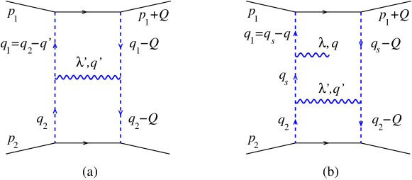
Figure 9: Emission from H diagram.

For the H-diagram (fig. 9.a), the CCV helicity amplitude [15] for emitting a graviton of momentum ${\boldsymbol{q}}^{\prime}={\boldsymbol{q}}_{2}-{\boldsymbol{q}}_{1}$ and helicity $\lambda^{\prime}$, in the center of mass frame with incident momentum along the $\hat{z}$-axis, is given by [cf. eq. (2.11)]

$$M_{\mathrm{Regge}}({\boldsymbol{q}}^{\prime},E,\omega,{\boldsymbol{q}}_{2}) =\frac{\kappa^{2}s^{2}J_{L}^{\mu\nu}\epsilon_{\mu\nu}^{(\lambda^{\prime})}}{({\boldsymbol{q}}-{\boldsymbol{q}}_{2})^{2}{\boldsymbol{q}}_{2}^{2}}=\frac{\kappa^{3}s^{2}}{{\boldsymbol{q}}^{\prime}{}^{2}}F^{(\lambda^{\prime})}({\boldsymbol{q}}_{2},{\boldsymbol{q}}_{2}-{\boldsymbol{q}}^{\prime})$$

$$F^{(\lambda)}({\boldsymbol{q}}_{2},{\boldsymbol{q}}_{1}) \equiv 1-\mathrm{e}^{\mathrm{i}\lambda(\phi_{{\boldsymbol{q}}_{2}}-\phi_{{\boldsymbol{q}}_{1}})}\;.$$ (3.13)

Correspondingly, the overlap-function (fig. 9.a), at generally non vanishing momentum transfer ${\boldsymbol{Q}}$, and for incidence direction along the $\hat{z}$-axis in the center of mass frame, is proportional to the Lipatov graviton kernel [29]

$$K({\boldsymbol{q}}_{2},{\boldsymbol{q}}_{1};{\boldsymbol{Q}})\equiv\sum_{\lambda^{\prime}}J_{L}^{\mu\nu}({\boldsymbol{q}}_{1},{\boldsymbol{q}}_{2})\epsilon_{\mu\nu}^{(\lambda^{\prime})}({\boldsymbol{q}}^{\prime})J_{L}^{\mu^{\prime}\nu^{\prime}}({\boldsymbol{q}}^{\prime}_{1},{\boldsymbol{q}}^{\prime}_{2})\epsilon_{\mu^{\prime}\nu^{\prime}}^{(\lambda^{\prime})*}({\boldsymbol{q}}^{\prime})\;,$$ (3.14)

where $J_{L}$ is the Lipatov current [29] and ${\boldsymbol{q}}^{\prime}_{i}\equiv{\boldsymbol{q}}_{i}-{\boldsymbol{Q}}:i=1,2$. In two transverse dimensions, where the ${\boldsymbol{q}}_{i}$’s are all coplanar, the explicit result is

$$K({\boldsymbol{q}}_{2},{\boldsymbol{q}}_{1};{\boldsymbol{Q}})=\frac{4\,{\boldsymbol{q}}_{1}^{2}\,{\boldsymbol{q}}_{2}^{2}\,{\boldsymbol{q}}^{\prime}_{1}{}^{2}\,{\boldsymbol{q}}^{\prime}_{2}{}^{2}}{[({\boldsymbol{q}}_{1}-{\boldsymbol{q}}_{2})^{2}]^{2}}2\sin\phi_{12}\sin\phi_{1^{\prime}2^{\prime}}\cos(\phi_{12}-\phi_{1^{\prime}2^{\prime}})$$ (3.15)

and checks with ref. [29].

The result (3.15) is valid for on-shell intermediate particles, and provides directly, by integration over ${\boldsymbol{q}}_{i}$ and Fourier transform in ${\boldsymbol{Q}}$ to ${\boldsymbol{b}}$-space, the imaginary part of the H-diagram amplitude, or [9]

$$\Im\delta_{H}(b,s)\equiv YGsR^{2}\int\mathrm{d}^{2}{\boldsymbol{q}}^{\prime}\;\left|\tilde{h}({\boldsymbol{b}},{\boldsymbol{q}}^{\prime})\right|^{2}\;,$$ (3.16)

where

$$\tilde{h}({\boldsymbol{b}},{\boldsymbol{q}})=2\int\frac{\mathrm{d}^{2}{\boldsymbol{q}}_{2}}{(2\pi)^{2}}\;\frac{\mathrm{e}^{\mathrm{i}{\boldsymbol{b}}\cdot{\boldsymbol{q}}_{2}}}{|{\boldsymbol{q}}|^{2}}\left[1-\mathrm{e}^{2\mathrm{i}(\phi_{{\boldsymbol{q}}_{2}-{\boldsymbol{q}}}-\phi_{{\boldsymbol{q}}_{2}})}\right]\;,$$ (3.17)

is the $h$-field in ${\boldsymbol{q}}$-space at $\lambda^{\prime}=-2$ [15, 19]. The quantity (3.17) has a logarithmic divergence, because of the known residual infrared singularity $\sim 1/{\boldsymbol{q}}^{\prime}{}^{2}$ of the integrand in (3.16), due to the LT polarization. Such divergence is expected and is compensated in observables by real emission in the usual way, so as to lead to finite, but resolution dependent results.

On the other hand, we are looking for $\Re\delta_{2}$, the H-diagram contribution to the 2-loop eikonal, which is supposed to be IR safe, because a ${\boldsymbol{b}}$-dependent IR divergence would be observable, and inconsistent with the Block-Nordsieck factorization theorem. In [7] it was shown that fixed order dispersion relations plus $S$-matrix exponentiation lead indeed to the finite result

$$\Re\delta_{2}(b,s)=\left.\frac{\pi}{2Y}\Im\delta_{H}(b,s)\right|_{\mathrm{Reg}}=\frac{\pi}{2}GsR^{2}\int\mathrm{d}^{2}{\boldsymbol{q}}^{\prime}\;\left|\tilde{h}({\boldsymbol{b}},{\boldsymbol{q}}^{\prime})\right|^{2}_{\mathrm{Reg}}\stackrel{{\scriptstyle b\gg R}}{{=}}{\alpha_{G}}\frac{R^{2}}{2b^{2}}=\frac{2G^{3}s^{2}}{b^{2}}\;.$$ (3.18)

Here the regularization subtraction is due to the second order contributions of $\delta_{0}$ and $\delta_{1}$ to the $S$-matrix exponential.

Our present purpose is actually to compute the graviton radiation associated to the H-diagram, in which a further Regge graviton vertex is introduced in all possible ways, as in fig 9.b for the upper-left corner. In the limit $|{\boldsymbol{q}}|=\hbar\omega\ll E$ — that we assume throughout the paper — the dominant contributions are for $|{\boldsymbol{q}}|\ll|{\boldsymbol{q}}^{\prime}|\sim m_{P}$, so that no insertions on the ${\boldsymbol{q}}^{\prime}$-exchange should be considered. As a consequence, for $q$ in jet 1 and using the CCV gauge [15] in which jet 2 is switched off, only the upper-left and upper-right insertions will be considered.

Consider first the upper-left diagram (fig. 9.b) at imaginary part level. For any fixed values of ${\boldsymbol{q}}$, ${\boldsymbol{q}}^{\prime}$ and ${\boldsymbol{Q}}$, the integrand has the form

$$\sqrt{{\alpha_{G}}}R\int\mathrm{d}^{2}{\boldsymbol{q}}_{s}\;\mathrm{e}^{\mathrm{i}{\boldsymbol{Q}}\cdot{\boldsymbol{b}}} \left(\frac{1}{{\boldsymbol{q}}^{\prime}{}^{2}}\right)^{2}F^{(\lambda^{\prime})}({\boldsymbol{q}}^{\prime}_{s}+{\boldsymbol{q}}^{\prime},{\boldsymbol{q}}^{\prime}_{s})F^{(\lambda^{\prime})}({\boldsymbol{q}}_{s}+{\boldsymbol{q}}^{\prime},{\boldsymbol{q}}_{s})$$

$$\times\kappa\frac{|q_{s}|^{2}}{|q|^{2}}\left(1-\frac{q_{s}^{*}}{q_{s}}\frac{q_{s}-q}{q_{s}^{*}-q^{*}}\right)+\cdots\;,$$ (3.19)

where ${\boldsymbol{q}}_{s}\equiv{\boldsymbol{q}}_{2}-{\boldsymbol{q}}^{\prime}$, ${\boldsymbol{q}}^{\prime}_{s}={\boldsymbol{q}}_{s}-{\boldsymbol{Q}}$, and we have taken, for definiteness, $\lambda=-2$. The $|q_{s}|^{2}$ factor in the numerator is needed in order to have the proper counting of $|q_{i}|^{2}$ denominators in multi-Regge factorization [29].

We then apply to eq. (3.19) the same reasoning used in sec. 2.2 to match the soft and Regge limits. By the approximate identity

$$\frac{|q_{s}|^{2}}{|q|^{2}}\left(1-\frac{q_{s}^{*}}{q_{s}}\frac{q_{s}-q}{q_{s}^{*}-q^{*}}\right)\simeq\frac{qq_{s}^{*}-q^{*}q_{s}}{q}\left[\frac{1}{q^{*}-\frac{\hbar\omega}{E}q_{s}^{*}}-\frac{1}{q^{*}-q_{s}^{*}}\right]\;,$$ (3.20)

valid in the region $(\hbar\omega/E)|q_{s}|\ll|q|$, we derive the relationship between Regge and soft insertion analogous to eqs. (2.13) and (2.25)

$$\text{Regge}|_{E}=\text{soft}|_{E}-\text{soft}|_{\hbar\omega}\;,$$ (3.21)

in which

$$\text{soft}|_{E}=\frac{\hbar\omega}{E}[\mathrm{e}^{2\mathrm{i}(\phi_{{\boldsymbol{q}}-\frac{\hbar\omega}{E}{\boldsymbol{q}}_{s}}-\phi_{{\boldsymbol{q}}})}-1]$$ (3.22)

for the upper-left case. A similar relationship holds for the upper-right case and, by including both jets, for any soft insertions, as pictured in fig. 10.

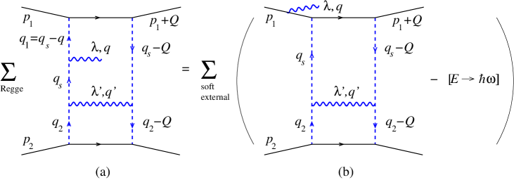
Figure 10: Diagrammatic representation of the soft-based emission amplitude.

We note at this point that in eq. (3.21) the insertion factor for the intermediate particle $p_{1}+q_{s}$ cancels out between left and right insertions, so that we get in total the insertion factor for external legs only, in the form

$$\kappa\left[\frac{E}{\hbar\omega}\left(\frac{q^{*}}{q}\frac{q-\frac{\hbar\omega}{E}Q}{q^{*}-\frac{\hbar\omega}{E}Q^{*}}-1\right)-\{E\to\hbar\omega\}\right]$$

$$\qquad\qquad=\kappa\left[\frac{E}{\hbar\omega}\left(\mathrm{e}^{2\mathrm{i}(\phi_{{\boldsymbol{q}}-\frac{\hbar\omega}{E}{\boldsymbol{Q}}}-\phi_{\boldsymbol{q}})}-1\right)-\left(\mathrm{e}^{2\mathrm{i}(\phi_{{\boldsymbol{q}}-{\boldsymbol{Q}}}-\phi_{\boldsymbol{q}})}-1\right)\right]\;.$$ (3.23)

The latter replaces in eq. (3.19) the sum of Regge insertions and is only dependent on the overall momentum transfer $Q$ (fig. 10).

Since the above factorization in ${\boldsymbol{Q}}$-space holds for any fixed values of ${\boldsymbol{Q}}$ and $|{\boldsymbol{q}}^{\prime}|>|{\boldsymbol{q}}|$, it is presumably valid for the IR regularization procedure of eq. (3.18) also, because the latter consists in subtracting the IR singularity due to lower order eikonal contributions to the $S$-matrix exponential. We shall then assume eq. (3.23) for the full graviton emission amplitude associated to H-diagram exchange. This leads to the expression

$${\cal M}_{H}({\boldsymbol{b}},E,{\boldsymbol{q}}) =\sqrt{{\alpha_{G}}}\frac{R}{\pi}\int\frac{\mathrm{d}^{2}{\boldsymbol{Q}}}{2\pi}\;\tilde{\Delta}_{H}({\boldsymbol{Q}})\mathrm{e}^{\mathrm{i}{\boldsymbol{Q}}\cdot{\boldsymbol{b}}}$$

$$\quad\times\left[\frac{E}{\hbar\omega}\left(\mathrm{e}^{2\mathrm{i}(\phi_{{\boldsymbol{q}}-\frac{\hbar\omega}{E}{\boldsymbol{Q}}}-\phi_{\boldsymbol{q}})}-1\right)-\left(\mathrm{e}^{2\mathrm{i}(\phi_{{\boldsymbol{q}}-{\boldsymbol{Q}}}-\phi_{\boldsymbol{q}})}-1\right)\right]\;,$$ (3.24)

where ${\alpha_{G}}\tilde{\Delta}_{H}({\boldsymbol{Q}})$ is the (regularized) inverse Fourier transform of $\Re\delta_{2}(b)$ in eq. (3.18).

The main achievement of eq. (3.24) is its independence of the detailed structure of the H-diagram because of the factorization of the soft insertions in ${\boldsymbol{Q}}$-space. Therefore, it is the generalization of the soft-based representation of the unified amplitude to the next-to-leading eikonal exchange.

3.3 Soft-based representation and eikonal resummation

We have just argued that the single graviton emission amplitude associated to H-diagram exchange is provided by eq. (3.24) which is directly expressible in terms of the H-diagram amplitude in ${\boldsymbol{Q}}$-space. We can even use the $z$-representation for the phase transfers

$$\mathrm{e}^{2\mathrm{i}\phi_{{\boldsymbol{\theta}}}}-\mathrm{e}^{2\mathrm{i}\phi_{{\boldsymbol{\theta}}^{\prime}}}=-2\int\frac{\mathrm{d}^{2}{\boldsymbol{z}}}{{2\pi z^{*}}^{2}}\left(\mathrm{e}^{\mathrm{i}A{\boldsymbol{z}}\cdot{\boldsymbol{\theta}}}-\mathrm{e}^{\mathrm{i}A{\boldsymbol{z}}\cdot{\boldsymbol{\theta}}^{\prime}}\right)\;,\qquad(A\in\mathbb{R}^{*})$$ (3.25)

and, by exchanging the order of ${\boldsymbol{Q}}$- and ${\boldsymbol{z}}$-integrals we recast eq. (3.24) in the form

$${\cal M}=\sqrt{{\alpha_{G}}}\frac{R}{\pi}\mathrm{e}^{-2\mathrm{i}\phi_{\boldsymbol{\theta}}}\int\frac{\mathrm{d}^{2}{\boldsymbol{z}}}{2\pi z^{*2}}\;\mathrm{e}^{\mathrm{i}b{\boldsymbol{z}}\cdot{\boldsymbol{q}}}\left\{\frac{E}{\hbar\omega}\left[\Delta({\boldsymbol{b}}-\frac{\hbar\omega}{E}b{\boldsymbol{z}})-\Delta({\boldsymbol{b}})\right]-\left[\Delta({\boldsymbol{b}}-b{\boldsymbol{z}})-\Delta({\boldsymbol{b}})\right]\right\}\;,$$ (3.26)

where $\Delta=\Delta_{0}+\Delta_{H}$ and $\Delta_{H}({\boldsymbol{b}})=R^{2}/2b^{2}$, thus generalizing the soft-based representation of eq. (2.13) to the next-to-leading (NL) term. We shall base on eq. (3.26) the subsequent formulation of our radiation model.

We note immediately, however, that eq. (3.26) has a purely formal meaning in the region $|b{\boldsymbol{z}}-{\boldsymbol{b}}|=\mathcal{O}\left(R\right)$, because the H-diagram expression (3.18) breaks down whenever $R/b$ is not small. We are thus led to think that we have to know something about the behaviour of $\Delta({\boldsymbol{b}})$ in the large-angle regime $b\sim R$ before even writing the representation (3.26) we argued for.

That is precisely what the reduced action model — as summarized in sec. 3.1 — provides for us. Indeed it consists in the resummation of the multi-H diagrams (fig. 8) of the eikonal, which is the set of two-body irreducible diagrams without a rescattering subgraph. Such diagrams are expected to share with the NL term the property that the central subgraphs have energetic $q^{\prime}$-type exchanges, where $|q^{\prime}|$ is of the order of the Planck mass or larger, thus suppressing their contribution to soft insertions with $\omega\sim R^{-1}\sim m_{P}^{2}/E$.

For that reason we think, we can repeat the argument with peripheral Regge insertions elaborated before, and then use the soft-Regge identities (3.21) to derive the external-particles insertion formula (3.24) and the soft-based representation (3.26). As a result, we are now able to look at the integrals in eq. (3.26) in a realistic way by setting

$$2\Delta({\boldsymbol{b}})=\frac{2\delta({\boldsymbol{b}})}{{\alpha_{G}}}=-2\chi_{b}+1-\frac{1}{t_{b}}\;,$$ (3.27)

where $\delta({\boldsymbol{b}})$ is the irreducible eikonal function with ACV resummation (after factorization of the IR part $\sim\log L/b$), which extrapolates the NL behaviour to small values of $b\sim R$. The latter is given in terms of the solution (3.8) for the reduced-action model action, and $t_{b}=\tanh\chi_{b}$ and $\chi_{b}$ are determined by the matching condition of eq. (3.7).

The expressions (3.27) and (3.8) are now well-defined for $b^{2}>b_{c}^{2}=\frac{3\sqrt{3}}{2}R^{2}$, where the role of the singularity at $b=b_{c}$ will be discussed soon. The result (3.26) contains the resummed modulating function

$$\Phi_{\mathrm{R}}(\omega,{\boldsymbol{z}}) \equiv\frac{E}{\hbar\omega}\left[\Delta({\boldsymbol{b}}-\frac{\hbar\omega}{E}b{\boldsymbol{z}})-\Delta({\boldsymbol{b}})\right]-\left[\Delta({\boldsymbol{b}}-b{\boldsymbol{z}})-\Delta({\boldsymbol{b}})\right]$$

$$\stackrel{{\scriptstyle\hbar\omega\ll E}}{{\simeq}}-b\Delta^{\prime}(b)\hat{{\boldsymbol{b}}}\cdot{\boldsymbol{z}}+\Delta({\boldsymbol{b}})-\Delta({\boldsymbol{b}}-b{\boldsymbol{z}})\equiv\Phi_{\mathrm{R},\mathrm{cl}}({\boldsymbol{z}})$$ (3.28)

(yielding $\Phi_{\mathrm{cl}}$ of eq. (2.15) in the classical limit and large-$b$ region), which generalizes the expressions (2.14) and (2.23) for the leading term, and enters the corresponding soft field

$$h_{s}^{(\lambda)}(\omega,z)\equiv-\frac{\Phi_{\mathrm{R}}(\omega,{\boldsymbol{z}})}{\pi^{2}|z|^{2}\mathrm{e}^{\mathrm{i}\lambda\phi_{z}}}\;.$$ (3.29)

Next step is to sum up all single-graviton emission amplitudes from any of the $\langle n\rangle\sim{\alpha_{G}}\gg 1$ irreducible eikonal exchanges with ACV resummation, by taking into account two important effects: (a) The correct phase and ${\boldsymbol{q}}$-dependence for all various incidence angles and (b) the rescattering of the emitted graviton with the fast particles themselves.

Both effects can be taken into account by the generalized ${\boldsymbol{b}}$-space factorization formula explained in sec. 2.3 for the leading graviton exchange. By replacing ${\cal M}_{\mathrm{el}}=2\delta_{0}$ by $2\delta$, the resummed soft field of eq. (2.21) becomes

$$\frac{1}{z^{*2}}\Phi_{\mathrm{R}}(\omega,{\boldsymbol{z}})\frac{\mathrm{e}^{2\mathrm{i}\delta({\boldsymbol{b}}-\frac{\hbar\omega}{E}b{\boldsymbol{z}})}-\mathrm{e}^{2\mathrm{i}\left[\delta({\boldsymbol{b}})+\frac{\hbar\omega}{E}\left(\delta({\boldsymbol{b}}-b{\boldsymbol{z}})-\delta({\boldsymbol{b}})\right)\right]}}{2\mathrm{i}\left[\delta({\boldsymbol{b}}-\frac{\hbar\omega}{E}b{\boldsymbol{z}})-\delta({\boldsymbol{b}})-\frac{\hbar\omega}{E}\left(\delta({\boldsymbol{b}}-b{\boldsymbol{z}})-\delta({\boldsymbol{b}})\right)\right]}$$

$$=\frac{1}{z^{*2}}\frac{\mathrm{e}^{2\mathrm{i}\delta({\boldsymbol{b}})}}{2\mathrm{i}\omega R}\left[\mathrm{e}^{2\mathrm{i}\omega R\frac{E}{\hbar\omega}\left[\Delta({\boldsymbol{b}}-\frac{\hbar\omega}{E}b{\boldsymbol{z}})-\Delta({\boldsymbol{b}})\right]}-\mathrm{e}^{2\mathrm{i}\omega R\left[\Delta({\boldsymbol{b}}-b{\boldsymbol{z}})-\Delta({\boldsymbol{b}})\right]}\right]\;,$$ (3.30)

where we have canceled out the $\Phi_{\mathrm{R}}$ function at numerator with the same factor in the denominator, and factored out the eikonal $S$-matrix $\mathrm{e}^{2\mathrm{i}\delta({\boldsymbol{b}})}$.

By applying the definition (2.24), the full graviton emission probability amplitude becomes

$$\frac{\mathfrak{M}_{\lambda}({\boldsymbol{b}};\omega,{\boldsymbol{\theta}})}{\mathrm{e}^{\mathrm{i}\lambda\phi_{\boldsymbol{\theta}}}} =\sqrt{{\alpha_{G}}}\frac{R}{\pi}\int\frac{\mathrm{d}^{2}{\boldsymbol{z}}}{2\pi|z|^{2}\mathrm{e}^{\mathrm{i}\lambda\phi_{z}}}\frac{\mathrm{e}^{\mathrm{i}b{\boldsymbol{z}}\cdot{\boldsymbol{q}}}}{2\mathrm{i}\omega R}\left\{\mathrm{e}^{2\mathrm{i}\omega R\left[\Delta({\boldsymbol{b}}-b{\boldsymbol{z}})-\Delta({\boldsymbol{b}})\right]}-\mathrm{e}^{2\mathrm{i}\omega R\frac{E}{\hbar\omega}\left[\Delta({\boldsymbol{b}}-\frac{\hbar\omega}{E}b{\boldsymbol{z}})-\Delta({\boldsymbol{b}})\right]}\right\}$$

$$\simeq\sqrt{{\alpha_{G}}}\frac{R}{\pi}\int\frac{\mathrm{d}^{2}{\boldsymbol{z}}}{2\pi|z|^{2}\mathrm{e}^{\mathrm{i}\lambda\phi_{z}}}\frac{\mathrm{e}^{\mathrm{i}b\omega{\boldsymbol{z}}\cdot({\boldsymbol{\theta}}-{\boldsymbol{\Theta}}_{s})}}{2\mathrm{i}\omega R}\left(\mathrm{e}^{-2\mathrm{i}\omega R\Phi_{\mathrm{R},\mathrm{cl}}({\boldsymbol{z}})}-1\right)\;,$$ (3.31)

where ${\boldsymbol{\Theta}}_{s}({\boldsymbol{b}})\equiv-b\Delta^{\prime}(b){\boldsymbol{\Theta}}_{E}={\boldsymbol{\Theta}}_{E}/t_{b}$, ${\boldsymbol{\Theta}}_{E}\equiv-(2R/b)\hat{{\boldsymbol{b}}}$ and $\Phi_{\mathrm{R},\mathrm{cl}}$ is the classical limit of $\Phi_{\mathrm{R}}$ introduced in eq. (3.28).

We note that the $\omega R$-dependent correction factor to naive ${\boldsymbol{b}}$-factorization takes into account in a simple and elegant way both incidence angle dependence and elastic rescattering with the incident particles including ACV resummation too.

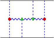
Figure 11: The first rescattering diagram contributing to the eikonal phase.

One may wonder at this point about the role of the rescattering contributions to the irreducible eikonal not included here in $\delta({\boldsymbol{b}})$, and starting at order $R^{4}/b^{4}$ (fig. 11). The latter presumably have a massless 3-body discontinuity and have thus the interpretation of $2\to 3\to 2$ transition in the rescattering process, leading to a recombination in a 2-body state. This would imply taking into account inelastic higher-order contributions to rescattering, a feature which is outside the scope of the present paper.

3.4 Coherent state and correlation effects

The derivation of the coherent-state operator proceeds now as in sec. 2.4 if we stick to the “linear” approximation, which neglects correlation effects. The only difference is the replacement of $\delta_{0}(b)$ by ${\alpha_{G}}\Delta({\boldsymbol{b}})$ in the amplitude $\mathfrak{M}_{\lambda}({\boldsymbol{b}},\vec{q})$ of eq. (3.31), so that we obtain

$$\hat{S}=\mathrm{e}^{2\mathrm{i}\delta({\boldsymbol{b}})}\exp\left\{\int\frac{\mathrm{d}^{3}q}{\sqrt{2\omega}}\;2\mathrm{i}\left(\sum_{\lambda}\mathfrak{M}_{\lambda}({\boldsymbol{b}},\vec{q})a_{\lambda}^{\dagger}(\vec{q})+\text{h.c.}\right)\right\}\;.$$ (3.32)

We shall base on eq. (3.32) most of the subsequent results. But we want to provide a preliminary discussion of the limits of that approximation and of the size of correlations that we can envisage. That is important for the ACV-resummed model, because we would like to describe sizeable scattering angles $\Theta_{s}\sim R/b\sim\mathcal{O}\left(1\right)$, while approaching the collapse regime.

We start noticing that many-body correlations are already present from start in the many-graviton states of sec. 2.4 and are in principle calculable. For instance, the 2-body correlation can be estimated from eq. (2.29) and is, order of magnitude like,

$$c_{12}\sim\mathfrak{M}_{1}\mathfrak{M}_{2}\big{(}|z_{1}|\omega_{1}R|z_{2}|\omega_{2}R\big{)}/{\alpha_{G}}\;.$$ (3.33)

We note also that the factors $|z_{i}|=|x_{i}/b|\sim 1/\sqrt{\omega_{i}R}$ are small in the dominant integration region for radiation (sec. 2.5) so that $c_{12}$ becomes of relative order $\sqrt{\omega_{1}\omega_{2}}/E\simeq 1/{\alpha_{G}}\ll 1$ for $\omega_{i}R\sim\mathcal{O}\left(1\right)$. This means that, within our assumptions, we can neglect finite order correlations.

One may wonder, however, whether correlated emission can be enhanced by multiplicity effects — not only those of the exchanged gravitons ($\langle n\rangle\sim{\alpha_{G}}$) — but also those of the emitted ones ($\langle N\rangle\sim{\alpha_{G}}\Theta_{s}^{2}$), a number which may be large, and even more for $\Theta_{s}=\mathcal{O}\left(1\right)$.

One such effect is certainly present, and is due to energy conservation. Even if energy transfer is explicitly considered in the treatment of rescattering in secs. 2.3 and 2.4, the kinematical constraints are not explicitly enforced. But such constraints are needed, because the expected average emitted energy $\langle\omega\rangle\equiv E/\langle N\rangle=R^{-1}\Theta_{s}^{-2}$ is of the order of the so-called classical cutoff [13, 19] and cannot be large if $\Theta_{s}$ increases up to $\mathcal{O}\left(1\right)$. This means that the larger values of $\omega R$ can be reached only for a smaller number of gravitons, thus distorting the calculation of inclusive distributions. That effect is therefore important, but can be included in the coherent state (3.32) and will be discussed in sec. 4.3.

Another kind of multiplicity effect — not included in (3.32) — comes from multi-graviton emission by a single exchange. A simple model for that is to consider soft emission which, according to [7], sec. 4, is described by the operator eikonal

$$\hat{\delta}_{\text{soft}}({\boldsymbol{b}},a_{\boldsymbol{q}}) ={\alpha_{G}}\int\frac{\mathrm{d}^{2}{\boldsymbol{q}}_{s}}{(2\pi)^{2}}\;\frac{\mathrm{e}^{\mathrm{i}{\boldsymbol{q}}\cdot{\boldsymbol{b}}}}{{\boldsymbol{q}}_{s}^{2}}\mathcal{U}_{\text{soft}}^{{\boldsymbol{q}}_{s}}(a_{\boldsymbol{q}})$$

$$\mathcal{U}_{\text{soft}}^{{\boldsymbol{q}}_{s}}(a_{\boldsymbol{q}}) \equiv\exp\left\{2\sqrt{G}\int\frac{\mathrm{d}^{3}q}{\sqrt{2\omega_{q}}}|{\boldsymbol{q}}_{s}|\frac{\sin(\phi_{\boldsymbol{q}}-\phi_{{\boldsymbol{q}}_{s}})}{|{\boldsymbol{q}}|b}\left[a_{\lambda}^{\dagger}({\boldsymbol{q}})-a_{\lambda}({\boldsymbol{q}})\right]\right\}\;.$$ (3.34)

Here we can see the nonlinear structure of the operator (3.34) as “coherent state of coherent states” in the soft limit. Its linear part agrees with the state (3.32) by the approximate form of

$$\mathfrak{M}\simeq\sqrt{{\alpha_{G}}}\frac{\Theta_{E}}{2\pi}\frac{\sin(\phi_{\boldsymbol{q}}-\phi_{{\boldsymbol{q}}_{s}})}{|{\boldsymbol{q}}|}J_{0}(|{\boldsymbol{q}}|b)\;,$$ (3.35)

which is valid in the region $(E/\hbar\omega)|{\boldsymbol{q}}|\gg|{\boldsymbol{q}}_{s}|\gg|{\boldsymbol{q}}|$ [19]. On the other hand, nonlinear effects in (3.34) are pretty small, because the exchanged graviton coupling ${\alpha_{G}}$ affects only the ${\boldsymbol{q}}_{s}$-dependence and not the ${\boldsymbol{q}}$-dependence. Therefore the single-exchange multiplicity $\langle N_{1}\rangle\sim\langle N\rangle/{\alpha_{G}}\sim\mathcal{O}\left(\Theta_{s}^{2}\right)$ is down by a factor ${\alpha_{G}}$ and yields a quite limited enhancement, if any. By comparison, the nontrivial feature of the state (3.32) is that, though being confined to one emitted graviton per exchange, it takes into account all exchanged graviton’s multiplicities and thus produces a reliable $\omega R$ dependence.

To conclude, we stick in the following to the linear coherent state (3.32) to describe the main radiation features, but we introduce energy conservation constraints also, to better understand the large $\omega R$ part when approaching the collapse regime.

4 Finite angle radiation and approach-to-collapse
regime

4.1 The emission amplitude in the sizeable angle region

In the following, we concentrate on the analysis of the amplitude (3.31) in the semi-hard frequency region $\omega R\gtrsim 1$, because the very soft gravitons ($\omega\ll b^{-1}$) are already well described by the approach of sec. 2.

In that region the behaviour of (3.31) is quite sensitive to the angular parameter $\Theta_{E}\equiv 2R/b$, which occurs in the amplitude in two ways: in the overall coupling $\Theta_{E}\sqrt{{\alpha_{G}}}$ and in the explicit expression for the action, which is actually most sensitive, because of the $b=b_{c}$ branch-cut (sec. 3.1). Note also the occurrence in the amplitude of $\Delta({\boldsymbol{b}}-b{\boldsymbol{z}})$, which may be in the non-perturbative regime in the integration region $|{\boldsymbol{b}}-b{\boldsymbol{z}}|\lesssim R$ in which its $S$-matrix factor may be exponentially suppressed as in eq. (3.11).

For the above reason, we shall cutoff the rescattering contributions by the requirement $|{\boldsymbol{b}}-b{\boldsymbol{z}}|>b_{c}$. If $\Delta({\boldsymbol{b}})$ is in the perturbative regime $\Theta_{E}\ll 1$, that change is subleading by a relative power of $R^{2}/b^{2}$, because of phase space considerations, and the approach remains perturbative. If instead $0<(b-b_{c})/b\ll 1$, the cutoff procedure can be extended to virtual corrections, by unitarizing the coherent-state operator, as usual, but our approach becomes non-perturbative. Finally, we shall not discuss at all — in this paper — the subcritical case $b\leq b_{c}$ by limiting ourselves to the $b\to b_{c}^{+}$ approach-to-collapse regime. Considering $b<b_{c}$ would raise a variety of physical effects at both elastic and inelastic level that deserve a separate investigation.

Since we limit ourselves to the $b\geq b_{c}$ case, we do not expect real problems with $S$-matrix unitarity, because the tunneling suppression of the elastic channel in eq. (3.11) is absent. Nevertheless, the associated radiation shows quite interesting features, especially in the approach-to-collapse regime $b\to b_{c}^{+}$, that will be illustrated in the following.

Starting from the energy emission distribution of type (2.40)

$$\frac{\mathrm{d}E^{\mathrm{GW}}}{\mathrm{d}\omega}=2Gs\frac{\Theta_{E}^{2}}{\pi^{2}}\int\frac{\mathrm{d}^{2}{\boldsymbol{z}}}{|z|^{4}}\;\left(\frac{\sin\omega R\Phi_{\mathrm{R},\mathrm{cl}}({\boldsymbol{z}})}{\omega R}\right)^{2}\qquad(\omega R\gtrsim 1)\;,$$ (4.1)

we shall therefore distinguish two cases, in the large $\omega R$ region:

• $\omega R\gg\left(1-\frac{b_{c}^{2}}{b^{2}}\right)^{-3/2}\equiv(2\beta)^{-3/2}$. That is the truly small-angle regime, far away from the critical region $1-\frac{b_{c}^{2}}{b^{2}}\to 0$, or not too close to it. In that case $\omega R$ is very large, which means very small $z$’s ($|y|^{2}\simeq|x|^{2}/\sqrt{\beta}\simeq\mathcal{O}\left(1/\omega R\right)$) so that the qualitative features of the radiation can be derived from the small-$z$ approximation of the modulating function

  $$\Phi_{\mathrm{R},\mathrm{cl}}\simeq-\frac{1}{2}\left[D_{2}(b)x^{2}-D_{1}(b)y^{2}\right]+\mathcal{O}\left(|z|^{3}\right)\;,$$ (4.2)

  where we have used the expansion

  $$\Phi_{\mathrm{R},\mathrm{cl}} =\Delta(b)-\Delta(|{\boldsymbol{b}}-b{\boldsymbol{z}}|)-\Delta^{\prime}(b){\boldsymbol{b}}\cdot{\boldsymbol{z}}$$ (4.3a)

  $$\simeq-\frac{1}{2}\frac{\partial^{2}\Delta}{\partial b_{i}\partial b_{j}}b^{2}z_{i}z_{j}=\frac{1}{2}\left[-\Delta^{\prime\prime}(b)b^{2}\hat{b}_{i}\hat{b}_{j}-b\Delta^{\prime}(b)(\delta_{ij}-\hat{b}_{i}\hat{b}_{j})\right]$$ (4.3b)

  yielding (by use of eqs. (3.7) and (3.8))

  $$D_{1}=-b\Delta^{\prime}(b)=\frac{1}{t_{b}}\;,\qquad D_{2}=b^{2}\Delta^{\prime\prime}(b)=\frac{1+t_{b}^{2}}{t_{b}(3t_{b}^{2}-1)}\;.$$ (4.4)

  Here we note that $D_{1}\simeq D_{2}\simeq 1$ for $b\gg b_{c}$, thus recovering eq. (2.45) discussed before, while $D_{1}\simeq\sqrt{3}$, $D_{2}\simeq\sqrt{2}\left(1-\frac{b_{c}^{2}}{b^{2}}\right)^{-1/2}$ for $\beta\ll 1$ [eq. (3.12)] and thus $D_{2}$ diverges for $\beta\to 0$. Correspondingly, we get a formula similar to (2.40):

  $$\frac{\mathrm{d}E_{\mathrm{cl}}^{\mathrm{GW}}}{\mathrm{d}\omega}=2Gs\frac{\Theta_{E}^{2}}{\pi}\int\frac{\mathrm{d}^{2}z}{\pi|z|^{4}}\;\left[\frac{\sin\left(\frac{\omega R}{2}(D_{2}x^{2}-D_{1}y^{2})\right)}{\omega R}\right]^{2}\;,$$ (4.5)

  where however we should assume $|x|^{2}/\sqrt{\beta}\ll|x|^{3/2}$ (or, $|x|\ll\beta$) whenever $\beta\ll 1$, because the actual behaviour of $\Delta({\boldsymbol{b}}-b{\boldsymbol{z}})$ is that of a branch cut with index $3/2$, with small convergence radius in the $x$-variable. We should therefore require $\omega R\gg\beta^{-3/2}\gg 1$, as stated, so that such regime actually disappears in the limit $\beta\to 0$.

• $1\ll\omega R\ll\beta^{-3/2}$. That region opens up in the critical regime $0<\beta\ll 1$ and is dominant for $\beta\to 0$. However the quadratic small-$z$ expansion is no longer valid in the $x$-variable (because of the divergent coefficient), and the dominant approximation in the $|y|\simeq|x|\ll 1$ region becomes of type

  $$-\Phi_{\mathrm{R},\mathrm{cl}}(z)\simeq-\Phi_{1}(x)\equiv 4\left[\frac{1}{3}(\beta-x)^{3/2}-\frac{1}{3}\beta^{3/2}+\frac{1}{2}x\sqrt{\beta}\right]\stackrel{{\scriptstyle|x|\ll\beta}}{{\simeq}}\frac{x^{2}}{2\sqrt{\beta}}\;,$$ (4.6)

  where we have neglected, for simplicity, the $y$-dependence. We thus obtain what we shall call the 1-dimensional approximation to $\Phi_{\mathrm{R}}$, which is easily derived by expanding all terms in the expression (3.28) of $\Phi_{\mathrm{R},\mathrm{cl}}$ for $0<\beta\ll 1$, both in $\beta$ and in ${\boldsymbol{z}}$ and making the $(b-b_{c})^{3/2}$ behaviour explicit by eq. (3.12).

  The striking feature of (4.6) is that, in the $\beta\ll|x|\ll 1$ region, the dominant small-$x$ behaviour is $\Phi_{1}\simeq(4/3)|x|^{3/2}$, reflecting the branch-cut of the ACV resummed action, which is responsible for the very large second derivative (large tidal force) in (4.3b). By inserting that behaviour in (4.1), the corresponding distribution becomes

  $$\left.\frac{1}{\sqrt{s}}\frac{\mathrm{d}E^{\mathrm{GW}}}{\mathrm{d}\omega}\right|_{\text{enhanced}}=\frac{\Theta_{c}^{2}}{\pi\omega}\left(\frac{\omega R}{3}\right)^{1/3}\Gamma(2/3)\;,\quad\Theta_{c}^{2}\equiv\Theta_{E}^{2}(b_{c})=\frac{8}{3\sqrt{3}}$$ (4.7)

  and falls off as $(\omega R)^{-2/3}$ only. That radiation enhancement is a direct consequence of the critical index $3/2$ of the action branch cut at $b=b_{c}$.

We thus realize that, with increasing $R/b$, we quit the small-angle, weak-coupling regime a) — in which the radiated energy fraction is small (of order $\Theta_{E}^{2}$) and shows at most a $\log(\omega_{M}R)$ dependence with an upper frequency cutoff $\omega_{M}$ — and we enter the strong-coupling regime b) in which such fraction increases like $\Theta_{E}^{2}(\omega_{M}R)^{1/3}$ thus endangering the energy-conservation bound.

The possible violation of energy-conservation — which is nevertheless taken into account at linear level in the $\omega$’s for rescattering — is related to the fact that the kinematical constraints are not explicitly incorporated in multi-graviton production amplitudes and that multi-particle correlations are neglected also. We shall introduce such constraints in sec. 4.3.

4.2 Radiation enhancement and scaling

4.2.1 Small-${\boldsymbol{z}}$ radiation spectrum

In this section we present plots of the resummed amplitude and of the corresponding radiated energy distribution obtained by numerical evaluation. In this way we confirm the asymptotic behaviours derived in sec. 4.1 and visualize the shape of such quantities in the transition regions.

Let us start by displaying the main features of the gravitational wave spectrum obtained with the ACV resummation in the classical limit $\hbar\omega\ll E$ but close to the collapse region $b\gtrsim b_{c}$. For $\omega R\gtrsim 1$ this is obtained by substituting the reduced-action model field (3.28) (actually its classical limit $\Phi_{\mathrm{R},\mathrm{cl}}$ of eq. (4.3a)) in place of its leading counterpart $\Phi$ inside eq. (2.40). The results for various values of $\beta$ are shown in fig. 12. According to the estimates in sec. 4.1, at smaller and smaller $\beta\ll 1$ there is a larger and larger intermediate region $1\ll\omega R\ll\beta^{-3/2}$ of reduced decrease of the frequency spectrum $\sim\omega^{-2/3}$, followed by the typical asymptotic $\omega^{-1}$ fall off at $\omega R\gg\beta^{-3/2}$. In order to better discriminate the two regimes, the spectrum has been multiplied by $(\omega R)^{2/3}$, so that in the intermediate enhanced region the curves are almost flat.

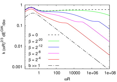
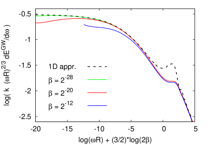
Figure 12: Left: the resummed spectrum for $\omega R\gtrsim 1$ in the approach-to-collapse regime $b\to b_{c}$ ($\beta\to 0$) for various values of $\beta$ ranging from $1/2$ ($b\to\infty$) to 0 ($b\to b_{c}$). The spectrum has been multiplied by $(\omega R)^{2/3}$ in order to highlight the enhancement in the intermediate regime $1\ll\omega R\ll\beta^{-3/2}$, followed by the asymptotic $1/\omega$ fall off. Right: some curves have been shifted horizontally and somewhat magnified in the neighbourhood of the transition region, showing the scaling behaviour with respect to the variable $a=(4\beta)^{3/2}\omega R$; the black-dashed curve represents the one-dimensional approximate representation (4.8). As usual, spectra are reduced by the factor $k=(Gs\Theta_{E}^{2})^{-1}$.

In the first plot of fig. 12 the black dot-dashed curve ($\beta=1/2$) represents the small-angle spectrum described in sec. 2.5. Decreasing the value of $\beta$ we obtain the solid curves (red, magenta, blue, green) and we observe the expected enhancement that amounts to a numerical factor of order one for $\omega R\lesssim 1$, but becomes much more important for large $\omega R\gtrsim 1$. It is also clear that the extension of the enhanced regime increases while decreasing $\beta$. In the limit $\beta\to 0$ the rescaled spectrum approaches the almost horizontal dashed line.

It is apparent that the shapes of the curves are quite similar at large $\omega R$, including the transition region between the enhanced and asymptotic regimes. By rescaling the independent variable $\omega R\to\omega R\beta^{3/2}$, the curves at small $\beta$ go on top of each other, as shown in the right plot of fig. 12. In other words, the asymptotic shape of the spectrum is a function of the single variable $a\equiv(4\beta)^{3/2}\omega R$. This scaling property can be understood by exploiting the small-$z$ expansion (4.6) that, substituted into eq. (2.40), provides the approximate representation

$$\frac{1}{Gs\Theta_{E}^{2}}(\omega R)^{2/3}\frac{\mathrm{d}E}{\mathrm{d}\omega} \simeq\frac{2}{\pi}a^{-1/3}\int_{-1}^{\infty}\mathrm{d}t\;\frac{\sin\left\{a\left[\frac{1}{3}\left((1+t)^{3/2}-1\right)-\frac{t}{2}\right]\right\}}{|t|(1+\sqrt{1+t})}\xrightarrow{a\to 0}\frac{2\Gamma(2/3)}{3^{1/3}\pi}$$

$$a \equiv(4\beta)^{3/2}\omega R$$ (4.8)

which depends only on the scaling variable $a$. This function is displayed in the black dashed line on the right plot of fig. 12, and it describes well the scaling behaviour in the enhanced region $a\ll 1$, and reasonably well the large-$\omega R$ region $a\gg 1$.

4.2.2 Angular behaviour

The angular behaviour of graviton radiation associated to large scattering angles $\Theta_{s}\sim 1$ can be obtained by numerical integration of the amplitude (3.31). However, in the main region of the spectrum, namely $\omega R\gtrsim 1$, it can be more conveniently described by using the small-$z$ approximation (4.2) of the modulating function $\Phi_{\mathrm{R},\mathrm{cl}}$. The main point here is that the two dispersion coefficients $D_{1}$ and $D_{2}$, which are equal for small scattering angle, become more and more different when approaching the critical angle $\Theta_{c}$. This fact causes the ensuing distribution of graviton radiation to be more and more directional, still concentrated at ${\boldsymbol{\theta}}\simeq{\boldsymbol{\Theta}}_{s}$, but with a larger dispersion, in particular along the $x$-direction, i.e., that of the scattering plane. This is clearly seen in fig. 13, where we compare on the ${\boldsymbol{A}}\equiv\sqrt{\omega R}\,\frac{{\boldsymbol{\theta}}-{\boldsymbol{\Theta}}_{s}}{|{\boldsymbol{\Theta}}_{s}|}$ plane the “isotropic” radiation (a) when $D_{1}=D_{2}=1$ with the “anisotropic” case (b) $D_{1}=\sqrt{3}$, $D_{2}=32$ (corresponding to $\beta\simeq 0.001$).

$A_{x}$    
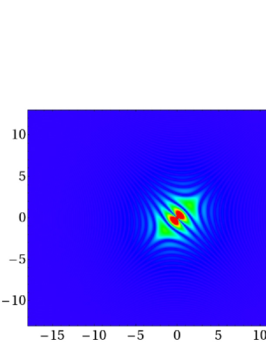
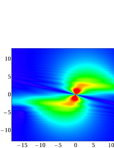
$A_{y}$                                           
         (a)                                                             (b)

Figure 13: Emission pattern of gravitational radiation for $\lambda=-2$ on the tangent space centered at ${\boldsymbol{\Theta}}_{s}$, parametrized by ${\boldsymbol{A}}\equiv\sqrt{\omega R}\,\frac{{\boldsymbol{\theta}}-{\boldsymbol{\Theta}}_{s}}{|{\boldsymbol{\Theta}}_{s}|}$. (a) the “isotropic” case $D_{1}=D_{2}$ discussed in sec. 2.5; (b) “anisotropic” case with $D_{1}=\sqrt{3}$, $D_{2}=32$.

We see, first of all, that in the collapse region (fig. 13b) the radiation is strongly enhanced, still keeping its correlation with the outgoing particle 1’ in the overall picture of the two jets. Furthermore, the larger dispersion in $\theta_{x}$ compared to $\theta_{y}$ gives a rationale for the 1-dimensional approximation (4.8) in the conjugated variables $x$ and $y$. Finally, such features are valid for any given frequency range $\Delta\omega$ and are thus somewhat independent of their relative normalization, which is possibly affected by energy-conservation constraints, to be discussed next.

4.3 Energy-conservation and “temperature”

In order to take into account energy-conservation constraints, we shall calculate coherent-state amplitudes and distributions by setting — event by event — the explicit energy bound $\sum_{i=1}^{N}\hbar\omega_{i}<E$, in which we refer to a single “jet”, say along $p_{1}$. Such bounds are effectively extended to virtual corrections by a factorization assumption, as proposed by [23] on the basis of the AGK [34] cutting rules (see also sec. 4.3 of ref. [5]).

More explicitly, we modify the original independent-particle distributions (2.37) in a radiation sample of energy up to $E$ by introducing the corresponding kinematical bounds together with a rescaling factor $1/N(E)$ in probability (or $1/\sqrt{N(E)}$ in amplitude) to be determined by unitarity. For instance, by considering for simplicity the $\omega$-variables only, we define the energy-conserving distributions

$$\tilde{P}_{0}=\frac{P_{0}}{N(E)}\;,\qquad\mathrm{d}\tilde{P}(\{\omega_{i}N_{i}\})=\frac{P_{0}}{N(E)}\prod_{i}\frac{[p(\omega_{i})\Delta(\omega_{i})]^{N_{i}}}{N_{i}!}\Theta\Big{(}E-\sum_{i}\hbar\omega_{i}N_{i}\Big{)}\;,$$ (4.9)

where the $p(\omega)$ density is given by (2.38), with the amplitude $\mathfrak{M}_{\lambda}({\boldsymbol{b}},\vec{q})$ in (3.31). We have also discretized the Fock space in regions of extension $\Delta(\omega_{i})$, containing a number of gravitons $N_{i}$ each.

The normalization factor $N(E)>0$ in (4.9) is determined by the unitarity condition $\sum_{\{N_{i}\}}\tilde{P}(\{N_{i}\})=1$ and takes the form [cf. eq. (2.37)]

$$N(E)=\int_{-\mathrm{i}\infty}^{+\mathrm{i}\infty}\frac{\mathrm{d}\lambda}{2\pi\mathrm{i}}\;\frac{\mathrm{e}^{\lambda E}}{\lambda+\varepsilon}\exp\left\{\int_{0}^{\infty}\mathrm{d}\omega\;p(\omega)\left[\mathrm{e}^{-\omega\lambda}-1\right]\right\}$$ (4.10)

which carries the energy-conservation constraints and is obtained by summing over all events the (positive) partial probabilities. We stress the point that $E$ in eq. (4.10) is the energy available for the measures being considered, so that $E=\sqrt{s}/2$ if we consider the whole jet, but becomes $\sqrt{s}/2-\hbar\omega$ if we consider events associated to an observed graviton $\omega$ in that jet, and so on. On the basis of eqs. (4.9) and (4.10) it is straightforward to obtain, for the inclusive distributions,

$$\frac{\mathrm{d}\mathcal{N}}{\mathrm{d}\omega}=p(\omega)\frac{N(E-\hbar\omega)}{N(E)}\;,\qquad\frac{\mathrm{d}^{2}\mathcal{N}}{\mathrm{d}\omega_{1}\mathrm{d}\omega_{2}}=p(\omega_{1})p(\omega_{2})\frac{N(E-\hbar\omega_{1}-\hbar\omega_{2})}{N(E)}$$ (4.11)

and so on. We notice also that virtual corrections are explicitly incorporated in (4.10) via the normal-ordering of the state (3.32) [cf. eq. (2.36)], and that $N(E)$ is actually infrared safe.

The main point is now that the inclusive distributions (4.11) carry $N(E)$-dependent correction factors due to the phase-space restrictions $E\to E-\hbar\omega,\cdots$, and so on, that will turn out to suppress the large-$\omega R$ region by an exponential cutoff. Arguments for a cutoff are provided also in the approach of ref. [16] to the transplanckian scattering without impact parameter identification of ref. [14].

In order to estimate $N(E)$ it is convenient to rewrite it in terms of the quantity ($\lambda\equiv R\tau$)

$$\frac{\langle\hbar\omega\rangle_{\tau}}{\sqrt{s}/2}\equiv F(\tau)=\int_{0}^{\infty}\mathrm{d}\omega\;\frac{\hbar\omega}{\sqrt{s}/2}p(\omega)\mathrm{e}^{-\omega R\tau}\;,$$ (4.12)

which represents the (exponentially weighted) radiated-energy fraction, given in our case (3.31) by [cf. eq. (4.1)]

$$F(\tau)=\frac{\Theta_{E}^{2}}{\pi^{2}}\int\frac{\mathrm{d}^{2}z}{|z|^{4}}\int_{0}^{\infty}\frac{\sin^{2}(\omega R\Phi_{\mathrm{R},\mathrm{cl}})}{(\omega R)^{2}}\mathrm{e}^{-\omega R\tau}\mathrm{d}(\omega R)\;.$$ (4.13)

We then obtain from eq. (4.10) (${\alpha_{G}}=R\sqrt{s}/2=Gs$) the expression

$$N(E)=\text{const}\int_{\varepsilon-\mathrm{i}\infty}^{\varepsilon+\mathrm{i}\infty}\mathrm{d}\tau\;\exp\left\{ER\tau-\log\tau-{\alpha_{G}}\int_{0}^{\tau}F(\tau^{\prime})\;\mathrm{d}\tau^{\prime}\right\}$$ (4.14)

and we proceed to estimate it by the saddle-point method. The saddle point value $\bar{\tau}>0$ is determined by the equation ($E=\sqrt{s}/2$)

$$F(\bar{\tau})=1-\frac{1}{{\alpha_{G}}\bar{\tau}}\;,$$ (4.15)

which represents the share between emitted (l.h.s.) and preserved ($1/{\alpha_{G}}\bar{\tau}$) energy fractions at the saddle point exponent $\bar{\tau}$. Fluctuation corrections are also calculable (app. A) and will be discussed shortly.

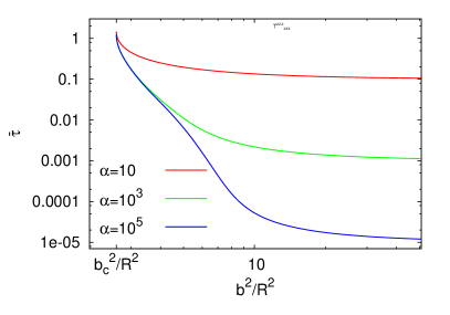
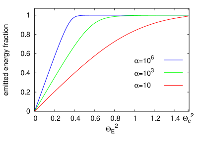
(a)                                                                 (b)

Figure 14: (a) Dependence of the saddle point $\bar{\tau}$ on the impact parameter $b^{2}$, for various values of ${\alpha_{G}}$; (b) emitted energy fraction vs $\Theta_{E}^{2}$ for various values of ${\alpha_{G}}$.

The numerical evaluation of (4.15) (fig. 14) is better understood by working out eq. (4.13) in the form

$$1-\frac{1}{{\alpha_{G}}\bar{\tau}}=F(\bar{\tau})=\frac{\Theta_{E}^{2}}{\pi^{2}}\int\frac{\mathrm{d}^{2}{\boldsymbol{z}}}{|z|^{4}}\;|\Phi(z)|I\left(\frac{2|\Phi({\boldsymbol{z}})|}{\bar{\tau}}\right)\;,$$ (4.16)

where, by explicit integration,

$$\tan\chi I(\tan\chi)=\chi\tan(\chi)+\frac{1}{2}\log(\cos^{2}\chi)\;,$$ (4.17)

The result shows that $\bar{\tau}\sim\mathcal{O}\left(1/{\alpha_{G}}\right)$ in the small-angle region ($b\gg R$), while $\bar{\tau}=\mathcal{O}\left(1\right)$ in the collapse regime. In between, the radiated energy fraction varies from 0 to 1.

In order to understand the role of $\bar{\tau}$ for the energy-conservation cutoff, we estimate the inclusive distribution (4.11) at the saddle point, and we find

$$\frac{\mathrm{d}\mathcal{N}}{\mathrm{d}\omega}=p(\omega)\mathrm{e}^{-(\bar{\tau}+\Delta\tau)\omega R}\;,$$ (4.18)

where the $\bar{\tau}$ term in the exponent comes from the explicit energy dependence of $N(E-\omega)$, and the correction $\Delta\tau$ comes from the implicit one through $\bar{\tau}(E-\omega)$, to which — by $\bar{\tau}$-stationarity — mostly fluctuations contribute. We show in app. A that this kind of corrections is sizeable when $\bar{\tau}=\mathcal{O}\left(1/{\alpha_{G}}\right)$ is small (where however the cutoff is not really important) while it is small when $\bar{\tau}=\mathcal{O}\left(1\right)$ is essential, that is in the approach-to-collapse regime. The cutoff exponent $\bar{\tau}$ has already been used in the definitions (4.13) and (4.16).

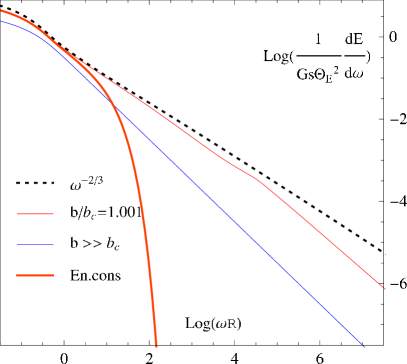
Figure 15: Frequency spectrum of graviton radiation in various contexts. Three curves have no energy conservation constraints, and correspond to: large $b/R$ where subleading effects are negligible (blue); $b$ close to the critical parameter $b_{c}$ where subleading effects causes the enhancement (thin red); limit $b\to b_{c}^{+}$ (dashed black). The last curve (thick red) shows the suppression due to energy conservation constraints in the case of $b$ close to $b_{c}$.

In more detail, it is useful to distinguish a very small angle regime $\Theta_{s}^{2}\ll\bar{\Theta}^{2}\equiv 1/\log{\alpha_{G}}$, in which $\bar{\Theta}^{2}$ acts as threshold for important energy-conservation effects like energy fractions of order 0.5, say [fig. 14.b and eq. (2.42)]. Below it, the radiated fraction $\sim\Theta_{s}^{2}$ is very small and so is $\bar{\tau}\sim 1/{\alpha_{G}}$. Furthermore, the exponent $\bar{\tau}+\Delta\tau\sim\Theta_{s}^{2}/{\alpha_{G}}$ is even smaller than $\bar{\tau}$ because of cancellations with the term $\Delta\tau$ (app. A), thus leading to negligible conservation corrections.

On the other hand, for $\Theta_{s}^{2}$ above $\bar{\Theta}^{2}$, both the exponent part $\bar{\tau}$ and the radiated fraction increase (fig. 14) up to $\mathcal{O}\left(1\right)$ for $\Theta_{E}^{2}\to\Theta_{c}^{2}=\mathcal{O}\left(1\right)$, while $\Delta\tau/\bar{\tau}$ becomes $\mathcal{O}\left(1/{\alpha_{G}}\right)\ll 1$, that is, small.

In that case — of strong coupling and radiation enhancement — the whole energy is radiated off, and this fact fixes $\bar{\tau}=\tau_{c}=1.2$ in a rather precise way. Furthermore, the same exponent (with $\Delta\tau/\bar{\tau}\sim 1/{\alpha_{G}}\ll 1$) occurs in all the graviton distributions (4.11) which — because of such approximate universality — turn out to be approximately factorized and thus weakly correlated, even after the inclusion of energy conservation. In other words, while the rescaling factor $\sqrt{N(E)}$ keeps the phase relations of the coherent state (3.32) among the various $\omega$-bins, it also introduces, by the $E$-dependence of (4.10) and the $\omega$-dependence of (4.11), an almost universal frequency cutoff parameter $R^{-1}$, a “quasi-temperature” we would say, in the approach-to-collapse regime. Numerically, the exponent $\tau_{c}R$ turns out to be of the order of the inverse Hawking temperature for a black hole mass $\simeq 0.1\sqrt{s}$, notably smaller than $\sqrt{s}$, and the corresponding spectrum — in each one of the two jets with $E=\sqrt{s}/2$ that our radiation consists of — is given in fig. 15.

Our semiclassical method does not allow, at present, a precise interpretation of the features just mentioned in terms of black hole physics, mostly because of our ignorance of what a black hole really is in quantum physics. Nevertheless we think that, applying our soft-based representation to the approach-to-collapse regime, we have constructed a coherent radiation sample which shares some of its properties with a Hawking radiation, thus suggesting a deeper relationship. That fact, because of coherence, goes in the direction of a quantum theory overcoming the information paradox, even if the details of such relationship are not known yet.

5 Outlook

The main technical progress presented here is the extension of the semiclassical graviton radiation treatment in transplanckian scattering to cover finite scattering angles $\sim R/b$. That result is in turn based on the ACV eikonal resummation and on the validity — for such reduced-action model — of the soft-based representation of the radiation amplitude argued for in sec. 3.

After such steps, we are really able to follow the approach to the classical collapse regime by a fully explicit, unitary coherent state, given the fact that collapse is signalled by a branch cut singularity of the action at $b=b_{c}=\mathcal{O}\left(R\right)$ with some scattering angle $\Theta_{c}=\mathcal{O}\left(1\right)$ and branch-cut index $3/2$. While $b_{c}$ and $\Theta_{c}$ are expected to be somewhat model-dependent, the index $3/2$ is expected to be robust because it yields the first non-analytic behaviour, by the action stationarity in the angular parameter $t_{b}$.

The first striking feature that we notice is that, because of the index $3/2$, the action has very large second derivatives (tidal forces) and thus yields a radiation enhancement causing about the whole-energy be radiated off for $b\to b_{c}^{+}$. Actually, it also requires the enforcement of the kinematical constraints in order to insure energy conservation.

Energy-conservation constraints (sec. 4) are introduced in real emission event by event and transferred to virtual corrections in some approximation which amounts to a factorization assumption, natural for the weakly correlated coherent-state that we have constructed. The outcome is that energy-conservation effects, which are negligible for $\Theta_{s}\ll 1$, are instead quite important in the approach-to-collapse regime, and provide an exponential suppression of the large $\omega R$ region. The latter is approximately universal, that is occurs in all the inclusive distributions, with small corrections and weak correlations, both depending on the parameter $1/{\alpha_{G}}$, where ${\alpha_{G}}=Gs/\hbar\gg 1$ is the magnitude of the final multiplicity.

The conclusive features just mentioned show that our radiation sample (corresponding to two jets with masses up to $\sqrt{s}/2$) — though coherent by construction — is characterized by an almost universal, exponential frequency cutoff close to $1/R$ which plays a role analogous to the Hawking temperature (at a mass notably smaller than $\sqrt{s}$). Such fact suggests a deeper relationship with the possible collapse dynamics, whose boundaries are however difficult to pinpoint, in view of both our approximations and our ignorance about the nature of a quantum black hole. We nevertheless think , because of coherence, that our results go in the direction of a quantum theory overcoming the information paradox, even if details of their relationship to black hole physics are not known yet.

6 Acknowledgments

It is a pleasure to thank Gabriele Veneziano for a number of interesting conversations on the topics presented in this paper, and Domenico Seminara for useful discussions. We also wish to thank the Galileo Galilei Institute for Theoretical Physics for hospitality while part of this work was being done.

Appendices

Appendix A Fluctuation corrections to inclusive distributions

It is straightforward to introduce a quadratic fluctuation expansion in eq. (4.14) to yield the normalization factor

$$N(E) =\int_{\bar{\tau}-\mathrm{i}\infty}^{\bar{\tau}+\mathrm{i}\infty}\frac{\mathrm{d}\tau}{2\pi\mathrm{i}}\;\exp\left\{ER\bar{\tau}-\log\bar{\tau}-{\alpha_{G}}\int_{0}^{\bar{\tau}}F(\tau^{\prime})\mathrm{d}\tau^{\prime}+\frac{1}{2}(\tau-\bar{\tau})^{2}\left[\frac{1}{\bar{\tau}^{2}}-{\alpha_{G}}F^{\prime}(\bar{\tau})\right]\right\}$$

$$\simeq\text{const}\exp\left\{\left[ER\bar{\tau}-{\alpha_{G}}\int_{0}^{\bar{\tau}}F(\tau^{\prime})\mathrm{d}\tau^{\prime}\right]-\frac{1}{2}\log\left(1-{\alpha_{G}}\bar{\tau}^{2}F^{\prime}(\bar{\tau})\right)\right\}\;.$$ (A.1)

We note that the $\log\bar{\tau}$ term cancels out, so that the overall size of fluctuations is determined by the function

$$f(\bar{\tau})\equiv-{\alpha_{G}}\bar{\tau}^{2}F^{\prime}(\bar{\tau})\simeq\begin{cases}\displaystyle\frac{\Theta_{E}^{2}}{2\pi}{\alpha_{G}}\bar{\tau}&(\Theta_{E}\ll 1)\\[11.38109pt] \displaystyle\frac{1}{3}{\alpha_{G}}\bar{\tau}^{2/3}\tau_{c}^{1/3}&(\Theta_{E}\simeq\Theta_{c})\;.\end{cases}$$ (A.2)

Although this function is pretty small (large) in the small (large) angle regime, its relative importance with respect to the exponent part $\bar{\tau}$ goes just in the opposite. In fact, in the small-$\bar{\tau}$ regime (where the cutoff is unimportant) the expansion of the remaining log term produces contributions of order comparable to those in square brackets.

To better understand this point, we combine eq. (A.1) with the saddle-point equations

$$ER={\alpha_{G}}F(\bar{\tau})+\frac{1}{\bar{\tau}}\;,\qquad\bar{\tau}^{\prime}(E)=-R\bar{\tau}^{2}\frac{1}{1+f(\bar{\tau})}$$ (A.3)

to get, after some algebra,

$$\left.\frac{\mathrm{d}\log N(E-\omega)}{\mathrm{d}E}\right|_{\omega=0} =R\bar{\tau}(E)+\left.\frac{\partial\log N}{\partial\bar{\tau}}\right|_{\bar{\tau}(E)}\bar{\tau}^{\prime}(E)$$

$$=R\bar{\tau}(E)\left[\frac{f(\bar{\tau})}{1+f(\bar{\tau})}+\frac{\bar{\tau}f^{\prime}(\bar{\tau})}{2(1+f(\bar{\tau}))^{2}}\right]=R\bar{\tau}\left(1+\frac{\bar{\tau}}{2}\frac{\partial}{\partial\bar{\tau}}\right)\left(\frac{f}{1+f}\right)\;.$$ (A.4)

Consider first the strong coupling regime in which $\bar{\tau}=\mathcal{O}\left(1\right)$. It is clear that $f(\bar{\tau})$ is $\mathcal{O}\left({\alpha_{G}}\right)$ so that

$$\frac{\mathrm{d}\mathcal{N}}{\mathrm{d}\omega}\simeq p(\omega)\mathrm{e}^{-\omega R(\bar{\tau}+\Delta\tau)}\simeq p(\omega)\mathrm{e}^{-\omega R\bar{\tau}}$$ (A.5)

with a correction

$$\frac{\Delta\tau}{\bar{\tau}}=\left(1+\frac{\bar{\tau}}{2}\frac{\partial}{\partial\bar{\tau}}\right)\left(\frac{-1}{1+f}\right)$$ (A.6)

which is small, $\Delta\tau/\bar{\tau}=\mathcal{O}\left(1/{\alpha_{G}}\right)$, leading to an approximately universal exponent $\bar{\tau}$.

On the other hand, in the weak coupling regime, $\Theta_{E}\ll 1$, $\bar{\tau}$ is small, starting $\mathcal{O}\left(1/{\alpha_{G}}\right)$ so that $f=\mathcal{O}\left(\Theta_{E}^{2}\right)$ is small too. As a consequence, relative corrections are large, so as to allow cancellations with the leading term and an even smaller exponent. That is fortunately unimportant, because energy conservation corrections are small in that regime. For instance, in the regime $\Theta_{E}^{2}\ll 1$ and $\bar{\tau}=\mathcal{O}\left(1/{\alpha_{G}}\right)$, we get

$$\bar{\tau}+\Delta\tau\simeq\bar{\tau}\frac{f}{1+f}=\mathcal{O}\left(\Theta_{E}^{2}/{\alpha_{G}}\right)\;,$$ (A.7)

yielding negligible corrections to the naive inclusive distribution. We conclude that for $\Theta_{E}\ll 1$ inclusive distributions avoid the energy-conservation cutoff, while for $\Theta_{E}\simeq\Theta_{c}=\mathcal{O}\left(1\right)$ such cutoff is provided by $\bar{\tau}$ and is approximately universal. The final multiplicity is provided by (A.5) and is of $\mathcal{O}\left({\alpha_{G}}\right)$ with a finite coefficient.

Appendix B One-dimensional integral representation of the amplitude at large $\boldsymbol{\omega R}$

We want to give a simple representation of the graviton emission amplitude for large $\omega R\gg 1$. According to the discussion in sec. 2.5, the emission amplitude $\mathfrak{M}$ is dominated by the small-$z$ region, where the modulation function $\Phi_{R}$ can be approximated by its quadratic expansion (4.2). We can therefore express $\mathfrak{M}$ in terms of the two-dimensional complex integral

$$I({\boldsymbol{A}})=\int\frac{\mathrm{d}^{2}Z}{2\pi\mathrm{i}}\;\frac{\mathrm{e}^{\mathrm{i}(ZA^{*}+Z^{*}A)}}{Z^{*2}}\left[\mathrm{e}^{\mathrm{i}(D_{2}x^{2}-D_{1}y^{2})}-1\right]\;,\qquad(Z=x+\mathrm{i}y)\;,$$ (B.1)

as in eq. (2.45). For the resummed amplitude we note the presence of the two dispersion coefficients $D_{1}$ and $D_{2}$ that are different for finite $b$.

Our aim here then is to provide a simple representation of $I({\boldsymbol{A}})$. Gaussian integration is possible by eliminating the double pole by derivation with respect to $A$:

$$-\frac{\partial^{2}}{\partial A^{2}}I(A,A^{*}) =\int\frac{\mathrm{d}x\,\mathrm{d}y}{2\pi\mathrm{i}}\;\mathrm{e}^{\mathrm{i}(2xA_{1}+2yA_{2})}\left[\mathrm{e}^{\mathrm{i}(D_{2}x^{2}-D_{1}y^{2})}-1\right]$$

$$=\frac{1}{2\mathrm{i}\sqrt{D_{1}D_{2}}}\mathrm{e}^{-\mathrm{i}\frac{A_{1}^{2}}{D_{2}}+\mathrm{i}\frac{A_{2}^{2}}{D_{1}}}=\frac{1}{2\mathrm{i}\sqrt{D_{1}D_{2}}}\mathrm{e}^{-\mathrm{i}\frac{(A+A^{*})^{2}}{4D_{2}}-\mathrm{i}\frac{(A-A^{*})^{2}}{4D_{1}}}$$

$$=\frac{\mathrm{e}^{\mathrm{i}A^{+}A^{-}}}{2\mathrm{i}\sqrt{D_{1}D_{2}}}\;,\qquad A^{\pm}\equiv\frac{A_{2}}{\sqrt{D_{1}}}\pm\frac{A_{1}}{\sqrt{D_{2}}}\;.$$ (B.2)

The integral can be reconstructed if we knew the boundary conditions.

An alternative method is to perform one of the $x$, $y$ integrals in (B.1) by noticing that the exponent is bilinear in $\xi,\eta\equiv\sqrt{D_{2}}x\mp\sqrt{D_{1}}y$, so that one variable $\xi$ or $\eta$ can be kept fixed and real, while the other is complexified and deformed on the pole. By using

$$x=\frac{\xi+\eta}{2\sqrt{D_{2}}}\;,\quad y=\frac{\eta-\xi}{2\sqrt{D_{1}}}\;,\quad x-\mathrm{i}y=\frac{\xi d+\eta d^{*}}{2\sqrt{D_{1}D_{2}}}\;,\quad d\equiv\sqrt{D_{1}}+\mathrm{i}\sqrt{D_{2}}=\sqrt{D_{1}+D_{2}}\mathrm{e}^{\mathrm{i}\chi}\;,$$

$$2{\boldsymbol{z}}\cdot{\boldsymbol{A}}=A_{1}\frac{\xi+\eta}{\sqrt{D_{2}}}+A_{2}\frac{\eta-\xi}{\sqrt{D_{1}}}=\xi\left(\frac{A_{1}}{\sqrt{D_{2}}}-\frac{A_{2}}{\sqrt{D_{1}}}\right)+\eta\left(\frac{A_{1}}{\sqrt{D_{2}}}+\frac{A_{2}}{\sqrt{D_{1}}}\right)$$

and integrating over $\eta$ at fixed real $\xi$ at the double pole $\eta=\mathrm{e}^{-\mathrm{i}2\gamma}\xi$, $\gamma=\pi/2-\chi$, we obtain (in the case $A^{+}>0$)

$$I =\int\frac{\mathrm{d}\xi\mathrm{d}\eta}{4\pi\mathrm{i}\sqrt{D_{1}D_{2}}}\;\frac{\mathrm{e}^{\mathrm{i}\eta\xi}-1}{(\xi d+\eta d^{*})^{2}}4D_{1}D_{2}\mathrm{e}^{\mathrm{i}\eta\left(\frac{A_{1}}{\sqrt{D_{2}}}+\frac{A_{2}}{\sqrt{D_{1}}}\right)+\mathrm{i}\xi\left(\frac{A_{1}}{\sqrt{D_{2}}}-\frac{A_{2}}{\sqrt{D_{1}}}\right)}$$

$$=\int_{-\infty}^{0}\mathrm{d}\xi\;\frac{2\mathrm{i}\sqrt{D_{1}D_{2}}}{d^{*}{}^{2}}\left[\mathrm{e}^{\mathrm{i}\xi\mathrm{e}^{-\mathrm{i}2\gamma}(\xi+A^{+})-\mathrm{i}\xi A^{-}}(\xi+A^{+})\Theta(\xi+A^{+})-\mathrm{e}^{\mathrm{i}\xi(\mathrm{e}^{-\mathrm{i}2\gamma}A^{+}-A^{-})}A^{+}\right]$$

$$=\frac{2\sqrt{D_{1}D_{2}}}{D_{1}+D_{2}}\left[\frac{\mathrm{e}^{-\mathrm{i}2\gamma}A^{+}}{\mathrm{e}^{-\mathrm{i}2\gamma}A^{+}-A^{-}}\,-\mathrm{i}\mathrm{e}^{-\mathrm{i}2\gamma}A^{+}{}^{2}\int_{0}^{1}\mathrm{d}\rho\;(1-\rho)\mathrm{e}^{-\mathrm{i}\mathrm{e}^{-\mathrm{i}2\gamma}A^{+}{}^{2}\rho(1-\rho)+\mathrm{i}\rho A^{+}A^{-}}\right]\;.$$ (B.3)

By performing a partial integration of the second term (so as to subtract the term linear in $\rho$ of the integrand) we finally obtain

$$I =\frac{2\sqrt{D_{1}D_{2}}}{D_{1}+D_{2}}\left[\frac{1}{2}\left(\mathrm{e}^{\mathrm{i}A^{+}A^{-}}-\frac{A^{-}+A^{+}\mathrm{e}^{-\mathrm{i}2\gamma}}{A^{-}-A^{+}\mathrm{e}^{-\mathrm{i}2\gamma}}\right)\right.$$

$$\qquad\qquad\qquad\left.-\frac{\mathrm{i}}{2}A^{+}(A^{+}\mathrm{e}^{-\mathrm{i}2\gamma}+A^{-})\int_{0}^{1}\mathrm{d}\rho\;\mathrm{e}^{-\mathrm{i}[A^{+}{}^{2}\mathrm{e}^{-\mathrm{i}2\gamma}\rho(1-\rho)-A^{+}A^{-}\rho]}\right]$$

$$=\frac{C}{2}\left[\mathrm{e}^{-\frac{\mathrm{i}}{2}(\mathcal{A}^{2}+\tilde{\mathcal{A}}^{2})}-\mathrm{i}\frac{\mathcal{A}}{\tilde{\mathcal{A}}}+\mathrm{i}\mathcal{A}\int_{-\mathrm{i}\tilde{\mathcal{A}}}^{\mathcal{A}}\mathrm{d}\mathcal{A}^{\prime}\mathrm{e}^{-\frac{\mathrm{i}}{2}(\tilde{\mathcal{A}}^{2}+\mathcal{A}^{\prime}{}^{2})}\right]$$ (B.4)

with the following variables:

$$\mathcal{A} \equiv\frac{\mathrm{i}}{\sqrt{2}}(A^{+}\mathrm{e}^{-\mathrm{i}\gamma}+A^{-}\mathrm{e}^{\mathrm{i}\gamma})=\sqrt{\frac{D_{1}+D_{2}}{2D_{1}D_{2}}}\left(A+A^{*}\frac{D_{1}-D_{2}}{D_{1}+D_{2}}\right)\;,$$ (B.5)

$$\tilde{\mathcal{A}} \equiv\frac{1}{\sqrt{2}}(A^{+}\mathrm{e}^{-\mathrm{i}\gamma}-A^{-}\mathrm{e}^{\mathrm{i}\gamma})=\sqrt{\frac{2}{D_{1}+D_{2}}}A^{*}$$ (B.6)

$$\mathcal{A}^{\prime} \equiv-\mathrm{i}\tilde{\mathcal{A}}+\mathrm{i}\sqrt{2}A^{+}\mathrm{e}^{-\mathrm{i}\gamma}\rho\;,\qquad C=\sin(2\gamma)=\frac{2\sqrt{D_{1}D_{2}}}{D_{1}+D_{2}}\;.$$ (B.7)

Finally, an integration by parts shows that $I$ is identically given by

$$I=-C\frac{\mathcal{A}}{2}\int_{-\mathrm{i}\tilde{\mathcal{A}}}^{\mathcal{A}}\frac{\mathrm{d}\mathcal{A}^{\prime}}{\mathcal{A}^{\prime}{}^{2}}\;\mathrm{e}^{-\frac{\mathrm{i}}{2}(\tilde{\mathcal{A}}^{2}-\mathcal{A}^{\prime}{}^{2})}\;.$$ (B.8)

• It is easily verified that eq. (B.8), with the identification (B.5), is the solution of the differential equation (B.2) with boundary condition $\mathcal{A}_{\mathrm{in}}=-\mathrm{i}\tilde{\mathcal{A}}$.

• If $D_{1}=1=D_{2}$, as in the case of the emission amplitude discussed in sec. 2.5, $C=1$, $\mathcal{A}=A$ and $\tilde{\mathcal{A}}=A^{*}$. In particular, eq. (B.8) reduces to eq. (2.47).

• $\mathcal{A}$ and $\tilde{\mathcal{A}}$ are not complex conjugate for $D_{1}\neq D_{2}$.

• The amplitude vanishes when the integration limits coincide, i.e., $\mathcal{A}=-\mathrm{i}\tilde{\mathcal{A}}$, corresponding to $A^{+}=A_{2}/\sqrt{D_{1}}+A_{1}/\sqrt{D_{2}}=0$, or equivalently $\phi_{A}=-\gamma$. In the limit $D_{1}=D_{2}$, such nodal line corresponds to the azimuthal direction $\phi_{A}=-\pi/4$, while $\gamma$ becomes possibly small for $D_{1}\ll D_{2}$, as depicted in fig. 13.

References

- [1] G. ’t Hooft, Phys.Lett. B198, 61 (1987).
- [2] I. J. Muzinich and M. Soldate, Phys.Rev. D37, 359 (1988).
- [3] D. Amati, M. Ciafaloni, and G. Veneziano, Phys.Lett. B197, 81 (1987).
- [4] D. J. Gross and P. F. Mende, Phys.Lett. B197, 129 (1987).
- [5] D. Amati, M. Ciafaloni, and G. Veneziano, Int.J.Mod.Phys. A3, 1615 (1988).
- [6] H. L. Verlinde and E. P. Verlinde, Nucl.Phys. B371, 246 (1992), arXiv:hep-th/9110017.
- [7] D. Amati, M. Ciafaloni, and G. Veneziano, Nucl.Phys. B347, 550 (1990).
- [8] D. Amati, M. Ciafaloni, and G. Veneziano, Nucl.Phys. B403, 707 (1993).
- [9] D. Amati, M. Ciafaloni, and G. Veneziano, JHEP 0802, 049 (2008), arXiv:0712.1209.
- [10] G. Marchesini and E. Onofri, JHEP 06, 104 (2008), arXiv:0803.0250.
- [11] G. Veneziano and J. Wosiek, JHEP 09, 023 (2008), arXiv:0804.3321.
- [12] G. Veneziano and J. Wosiek, JHEP 09, 024 (2008), arXiv:0805.2973.
- [13] A. Gruzinov and G. Veneziano, Class. Quant. Grav. 33, 125012 (2016), arXiv:1409.4555.
- [14] G. Dvali, C. Gomez, R. Isermann, D. Lüst, and S. Stieberger, Nucl.Phys. B893, 187 (2015), arXiv:1409.7405.
- [15] M. Ciafaloni, D. Colferai, and G. Veneziano, Phys. Rev. Lett. 115, 171301 (2015), arXiv:1505.06619.
- [16] A. Addazi, M. Bianchi, and G. Veneziano, (2016), arXiv:1611.03643.
- [17] L. N. Lipatov, Nucl. Phys. B365, 614 (1991).
- [18] S. B. Giddings, D. J. Gross, and A. Maharana, Phys. Rev. D77, 046001 (2008), arXiv:0705.1816.
- [19] M. Ciafaloni, D. Colferai, F. Coradeschi, and G. Veneziano, Phys. Rev. D93, 044052 (2016), arXiv:1512.00281.
- [20] G. F. Giudice, R. Rattazzi, and J. D. Wells, Nucl. Phys. B630, 293 (2002), arXiv:hep-ph/0112161.
- [21] V. S. Rychkov, private communication.
- [22] S. B. Giddings and V. S. Rychkov, Phys. Rev. D70, 104026 (2004), arXiv:hep-th/0409131.
- [23] H. Grigoryan and G. Veneziano, private communication.
- [24] S. W. Hawking, Commun. Math. Phys. 43, 199 (1975).
- [25] S. W. Hawking, The Information Paradox for Black Holes, 2015, arXiv:1509.01147.
- [26] M. Ciafaloni and D. Colferai, JHEP 1410, 85 (2014), arXiv:1406.6540.
- [27] X. O. Camanho, J. D. Edelstein, J. Maldacena, and A. Zhiboedov, (2014), arXiv:1407.5597.
- [28] S. Weinberg, Phys.Rev. 140, B516 (1965).
- [29] L. Lipatov, Sov.Phys.JETP 55, 582 (1982).
- [30] M. Ciafaloni and D. Colferai, JHEP 0811, 047 (2008), arXiv:0807.2117.
- [31] M. Ciafaloni and D. Colferai, JHEP 0912, 062 (2009), arXiv:0909.4523.
- [32] M. Ciafaloni, D. Colferai, and G. Falcioni, JHEP 1109, 044 (2011), arXiv:1106.5628.
- [33] P. Aichelburg and R. Sexl, Gen.Rel.Grav. 2, 303 (1971).
- [34] V. A. Abramovsky, V. N. Gribov, and O. V. Kancheli, Yad. Fiz. 18, 595 (1973), [Sov. J. Nucl. Phys.18,308(1974)].