Inelastic Charge Transfer Dynamics in Donor-Bridge-Acceptor Systems Using Optimal  Modes

Abstract

We present a novel ab initio approach for computing intramolecular charge and energy transfer rates based upon a projection operator scheme that parses out specific internal nuclear motions that accompany the electronic transition. Our approach concentrates the coupling between the electronic and nuclear degrees of freedom into a small number of reduced harmonic modes that can be written as linear combinations of the vibrational normal modes of the molecular system about a given electronic minima. Using a time-convolutionless master-equation approach, parameterized by accurate quantum-chemical methods, we benchmark the approach against experimental results and predictions from Marcus theory for triplet energy transfer for a series of donor-bridge-acceptor systems. We find that using only a single reduced mode–termed the “primary” mode, one obtains an accurate evaluation of the golden-rule rate constant and insight into the nuclear motions responsible for coupling the initial and final electronic states. We demonstrate the utility of the approach by computing the inelastic electronic transition rates in a model donor-bridge-acceptor complex that has been experimentally shown that its exciton transfer pathway can be radically modified by mode-specific infrared excitation of its vibrational mode.

I Introduction

Energy and electronic transport plays a central role in a wide range of chemical and biological systems. It is the fundamental mechanism for transporting the energy of an absorbed photon to a reaction center in light harvesting systems and for initiating a wide range of photo-induced chemical processes, including vision, DNA mutation, and pigmentation. The seminal model for calculating electron transfer rates was developed by Marcus in the 1950’sMarcus (1956, 1965, 1993).

$$k_{Marcus}=\frac{2\pi}{\hbar}|V_{ab}|^{2}\frac{1}{\sqrt{4\text{$\pi$}k_{B}T\lambda}}e^{-(\lambda+\Delta\epsilon)^{2}/4\text{$\lambda$}k_{B}T}.$$ (1)

where $\lambda$ is energy required to reorganize the environment following the transfer of an electron from donor to acceptor. and $\Delta\epsilon$ is the driving force for the reaction, as illustrated in Fig. 1. If we assume that the nuclear motions about the equilibrium configurations of the donor and acceptor species is harmonic, the chemical reactions resulting from energy or charge transfer events can be understood in terms of intersecting diabatic potentials as sketched. The upper and lower curves are the adiabatic potential energy surfaces describing the nuclear dynamics resulting from an energy or charge transfer event, taking the geometry of the donor state as the origin.

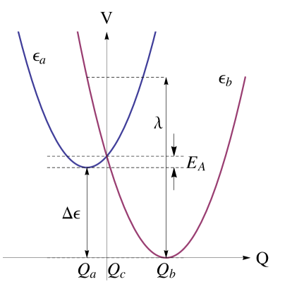
Figure 1: Sketch of Marcus parabolas for a model energy or charge transfer system. Labeled are the key parameters used to compute the Marcus rate constant (Eq. 1). Energies are given in eV and the collective nuclear displacement is dimensionless.

As the transfer occurs by crossing an energy barrier, the transfer rate can be expected to be in the Arrhenius form

$$k\propto e^{-E_{A}/k_{B}T},$$ (2)

with $E_{A}$ as the activation energy. Using $E_{A}={(\lambda+\Delta\epsilon)^{2}}/{4\lambda}$ we can relate the activation energy to both the reorganization energy and driving force, $-\Delta\epsilon$. One of the most profound predictions of the theory is that as the driving force increases, the transfer rate reaches a maximum and further increases in the driving force lead to lower reaction rates, termed the inverted regime. The existence of the inverted region was demonstrated unequivocally by Miller et al. Miller et al. (1984) in an elegant series of experiments that systematically tuned the driving force, reorganization energy, and diabatic coupling by careful chemical modification of the donor and acceptor.

A number of years ago, our group developed a time-convolutionless master equation approach for computing state-to-state rates in which the coupling between states depends upon the nuclear coordinatesPereverzev and Bittner (2006). This approach incorporates a fully quantum-mechanical treatment of both the nuclear and electronic degrees of freedom and recovers the well-known Marcus expression in the semiclassical limit. The model is parameterized by the vibrational normal mode frequencies, and the electronic energies and energy derivatives at a reference configuration. The approach has been used by our group to compute state-to-state transition rates in semi-empirical models for organic semiconducting light-emitting diode and photovoltaics Tamura et al. (2008, 2007); Bittner and Silva (2014); Singh et al. (2009).

We recently made a significant breakthrough in using this approach by tying it it to a fully ab initio quantum chemical approach for determining the diabatic states and electron/phonon coupling terms allowing unprecedented accuracy and utility for computing state-to-state electronic transition rates. Our methodology consists of two distinct components. The first is the use of a diabatization schemes for determining donor and acceptor states in a molecular unit. The other is a projection scheme which enables us to analyze the contribution of vibrations in reactions. Similar decomposition schemes have been presented by Burghardt Cederbaum et al. (2005); Gindensperger et al. (2006a, b) and the approach used here builds upon the method given in Ref. 13. We recently benchmarked this approach against both the experimental rates and recent theoretical rates presented by Subotnik et al. Subotnik et al. (2008, 2009, 2010) and successfully applied the approach to compute state-to-state transition rates in series of Pt bridged donor-acceptor systems recently studied by Weinstein’s group. We review here these latter results along with the details of our methods.

II Theoretical Approach

II.1 Model Hamiltonian

We consider a generic model for $n$ electronic states coupled linearly to a phonon bath. Taking the electronic ground state of the system as a reference and assuming that the electronic states are coupled linearly to a common set of modes, we arrive at a generic form for the Hamiltonian, here written for two coupled electronic states:

$$H=\left(\begin{array}[]{cc}\epsilon_{1}&0\\ 0&\epsilon_{2}\end{array}\right)+\left(\begin{array}[]{cc}{\mathbf{g}}_{11}&{\mathbf{g}}_{12}\\ {\mathbf{g}}_{21}&{\mathbf{g}}_{22}\end{array}\right)\cdot{\mathbf{q}}+\frac{{\mathbf{p}}^{2}}{2}+\frac{1}{2}\mathbf{q}^{T}\cdot\mathbf{\Omega}\cdot\mathbf{q}.$$ (7)

(8)

Here, the first term contains the electronic energies, $\epsilon_{1}$ and $\epsilon_{2}$ computed at a reference geometry–typically that of the donor or acceptor state. The second term represents the linearized coupling between the electronic and nuclear degrees of freedom given in terms of the mass-weighted normal coordinates $\mathbf{q}$. The diagonal terms give the adiabatic displacement forces between the reference geometry and the two states. If we choose one of the states as the reference state, then either $\mathbf{g}_{11}$ or $\mathbf{g}_{22}$ will vanish. The remaining two terms correspond to the harmonic motions of the nuclear normal modes, given here in mass-weighted normal coordinates. In the normal mode basis, the Hessian matrix, $\mathbf{\Omega}$, is diagonal with elements corresponding to the normal mode frequencies, $\omega_{j}^{2}$.

We now separate Eq. 8 into diagonal and off-diagonal terms

$$\hat{H}=\hat{H}_{o}+\hat{V}$$ (9)

and perform a polaron transform using the unitary transformation Grover and Silbey (1970); Rice and Gartstein (1994); Pereverzev and Bittner (2006).

$$U = e^{-\sum_{ni}\!\!\frac{g_{nni}}{\hbar\omega_{i}}|n\rangle\langle n|(a^{\dagger}_{i}-a_{i})}$$ (10)

$$= \sum_{n}|n\rangle\langle n|e^{-\sum_{i}\!\!\frac{g_{nni}}{\hbar\omega_{i}}(a^{\dagger}_{i}-a_{i})}$$

under which the transformed Hamiltonian is written in terms of the diagonal elements

$$\tilde{H}_{0}=U^{-1}H_{0}U=\sum_{n}\tilde{\epsilon}_{n}|n\rangle\langle n|+\sum_{i}\hbar\omega_{i}a^{\dagger}_{i}a_{i},$$ (11)

with the renormalized electronic energies,

$$\tilde{\epsilon}_{n}=\epsilon_{n}-\sum_{i}\frac{g_{nni}^{2}}{\hbar\omega_{i}},$$ (12)

and off-diagonal terms,

$$\hat{V}_{nm}=\sum_{i}g_{nmi}\left(a^{\dagger}_{i}+a_{i}-\frac{2g_{nni}}{\hbar\omega_{i}}\right)e^{\sum_{j}\frac{(g_{nnj}-g_{mmj})}{\hbar\omega_{j}}(a^{\dagger}_{j}-a_{j})}.$$ (13)

In the transformed (or dressed) picture the electronic transition from state $|n\rangle$ to $|m\rangle$ is accompanied by the excitations of all the normal modes.

At this point it is useful to connect the various terms in the phonon-dressed Hamiltonian with specific physical parameters. First, the reorganization energy is given by

$$\lambda_{nm}=\sum_{j}\frac{\left(g_{nnj}-g_{mmj}\right)^{2}}{\omega_{j}}=\sum_{j}\hbar\omega_{j}S_{j}$$ (14)

where the $\{S_{j}\}$ are the Huang-Rhys factors for each phonon mode. These are related to the Franck-Condon factor describing the overlap between the $v_{j}=1$ vibronic state in one electronic state with the $v_{j}=0$ vibronic state in the other. Likewise, the energy difference between the renormalized energy gaps is related to the driving force of the state-to-state transition,

$$\Delta E_{nm}=\tilde{\epsilon}_{n}-\tilde{\epsilon}_{m}.$$ (15)

Transforming to the interaction representation and performing a trace over the phonons gives the spectral density in terms of the autocorrelation of the electron-phonon coupling operators. Using the explicit form of the electron-phonon coupling operators, one can arrive at a compact expression for the autocorrelation function of the electron/phonon coupling

$$C_{nm}(t) = \langle V_{nm}V_{mn}(\tau)\rangle$$ (17)

$$= \sum_{i,j}g_{nmi}g_{mnj}\left(\left(\Delta_{nmi}(\overline{n}_{i}+1)e^{i\omega_{i}\tau}-\Delta_{nmi}\overline{n}_{i}e^{-i\omega_{i}\tau}+\Omega_{nmi}\right)\right.$$

$$\times\left.\left(\Delta_{nmj}(\overline{n}_{j}+1)e^{i\omega_{j}\tau}-\Delta_{nmj}\overline{n}_{j}e^{-i\omega_{j}\tau}+\Omega_{nmj}\right)\right.$$

$$\left.+\delta_{ij}(\overline{n}_{i}+1)e^{i\omega_{i}\tau}+\delta_{ij}\overline{n}_{i}e^{-i\omega_{i}\tau}\right)q_{nm}(\tau)f_{nm}(\tau),$$

Here, $\hat{V}_{nm}(t)$ is the electron-phonon coupling term in the Heisenberg representation and $\langle\cdots\rangle$ denotes a thermal average over the vibrational degrees of freedom. The remaining terms are constructed from the normal mode frequencies $\{\omega_{i}\}$ and electron/nuclear couplings $\{g_{nmi}\}$ viz.

$$\Delta_{nmi} = \frac{(g_{nni}-g_{mmi})}{\omega_{i}},$$ (18)

$$\Omega_{nmi} = \frac{(g_{nni}+g_{mmi})}{\omega_{i}},$$ (19)

$$q_{nm}(\tau) = e^{i\sum_{j}{\Delta^{2}_{nmj}\sin\omega_{j}\tau}},$$ (20)

$$f_{nm}(\tau) = e^{-2\sum_{j}(\overline{n}_{j}+\frac{1}{2})\Delta_{nmj}^{2}(1-\cos\omega_{j}\tau)}.$$ (21)

Finally, $\overline{n}_{i}$ is the Bose population of vibrational normal mode $i$,

$$\overline{n}_{i}=\frac{1}{e^{\beta\omega_{i}}-1}.$$ (22)

The spectral density and golden-rule rate can then be obtained by Fourier transform

$$S_{nm}(\tilde{\omega})=\int_{-\infty}^{\infty}\!\mathrm{d}te^{-i\tilde{\omega}t}\langle\hat{V}_{nm}(t)\hat{V}_{mn}(0)\rangle.$$ (23)

and

$$k_{nm}=2{\rm Re}\int_{0}^{\infty}\!\mathrm{d}t\left\langle\hat{V}_{nm}(0)\hat{V}_{mn}\left(t\right)\right\rangle e^{-i\tilde{\omega}_{nm}t}.$$ (24)

II.2 Non-Markovian Master Equation and Golden-Rule Rates

The formalism presented above requires both diagonal (${\mathbf{g}}_{nn}$) and off-diagonal (${\mathbf{g}}_{nm}$) derivative couplings between adiabatic states. Until recently, these couplings were difficult to impossible to compute for molecular systems using standard quantum chemical means. We next discuss how we have used the Edmiston-Ruedenberg (ER) localization scheme Edmiston and Ruedenberg (1963) to estimate the couplings. We also present how one can construct a reduced set of harmonic modes that fully capture the electron/nuclear coupling.

A workaround is to transform to a diabatic representation, whereby the Hamiltonian is written as

$$H_{dia} = U^{T}H_{adia}U$$ (27)

$$= \left(\begin{array}[]{cc}\epsilon_{a}(\mathbf{R})\mathrm{+T^{\prime}_{n}}(\mathbf{R})_{11}&V_{ab}\\ V_{ab}&\epsilon_{b}(\mathbf{R})\mathrm{+T^{\prime}_{n}}(\mathbf{R})_{22}\end{array}\right).$$

Fig. 2 shows a sketch of the adiabatic and diabatic potentials for a model two level system. While the adiabatic representation is precisely defined in terms of electronic eigenstates, the diabatic representation offers several advantages. First, the sharp derivative couplings that depend upon the nuclear velocity in the adiabatic representation are transformed to smoother diabatic couplings, $V_{ab}$ that only depend upon the nuclear positions. Second, potential energy surfaces are smoother and the avoided crossing is eliminated. A number of diabatization approaches have been developed and the reader is referred to Ref. 20 for a general review.

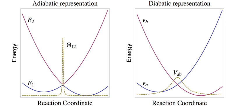
Figure 2: Sketch of adiabatic and diabatic representations for two-state system. Compared to adiabatic representations, diabatic representation has smoother energy surfaces and couplings.

The problem now is how to obtain the transformation matrix

$$U=\left(\begin{array}[]{cc}\cos\theta&\sin\theta\\ -\sin\theta&\cos\theta\end{array}\right).$$ (30)

While a number of methods are available a straightforward approach is to eliminate derivative coupling mathematically by requireing

$$\left\langle\phi_{i}(\mathbf{r};\mathbf{R})|\nabla_{\mathbf{R}}|\phi_{j}(\mathbf{r};\mathbf{R})\right\rangle=0.$$ (31)

However, this is computationally very expensive–especially for complex molecular systems, and exact solutions generally do not exist. Mead and Truhlar (1982)

An alternative approach is to use physical intuition rather than a purely mathematical constraint to define the diabatic states. The Edmiston-Ruedenberg (ER) diabatization scheme is such a scheme and is based on the idea that the diabatic states can be obtained by maximizing the total electron repulsion between localized states,

$$f_{ER}=\sum_{k}^{N_{states}}\int\int dr_{1}dr_{2}\frac{\left\langle\phi_{k}|\hat{\rho}\left(r_{1}\right)|\phi_{k}\right\rangle\left\langle\phi_{k}|\hat{\rho}\left(r_{2}\right)|\phi_{k}\right\rangle}{\left\|r_{1}-r_{2}\right\|}.$$ (32)

When the adiabatic (and diabatic) energy minima are far enough away from the crossing points and the mixing angles between the diabatic and adiabatic states is small, we can use the gradients of the adiabatic potentials to approximate the diabatic potentials. Thus, if we perform calculations at the optimized geometry of the final acceptor state (i. e. about $Q_{2}$ in Fig. 1), we can write the Hamiltonian as

$$H_{dia,e}=\left(\begin{array}[]{cc}\epsilon_{1}&V_{12}\\ V_{21}&\epsilon_{2}\end{array}\right)+\left(\begin{array}[]{cc}0&0\\ 0&1\end{array}\right){\mathbf{g}}_{22}\cdot{\mathbf{q}}+H_{osc},$$ (37)

where $H_{osc}$ is the harmonic oscillator Hamiltonian for the vibrational normal modes. The linear assumption amounts to performing a series expansion of the full, multi-dimensional coupling term and keeping only the lowest order terms. Systematic improvement can be made by including higher-order (e.g. quadratic) off-diagonal couplings. However, this would involve a substantial increase in the complexity of the theory. The linear assumption is reasonable so long as the mixing angle is small. Yang and Bittner (2014, 2015)

We obtain the diabatic couplings $V_{12}$ and the mixing angle $\theta$ via ER localization and transform the electronic Hamiltonian from the adiabatic basis to the diabatic basis viz.

$$H_{dia}=\left(\begin{array}[]{cc}\cos\theta&-\sin\theta\\ \sin\theta&\cos\theta\end{array}\right)\left(\begin{array}[]{cc}\epsilon_{1}&0\\ 0&\epsilon_{2}\end{array}\right)\left(\begin{array}[]{cc}\cos\theta&\sin\theta\\ -\sin\theta&\cos\theta\end{array}\right).$$ (38)

The diabatic coupling is then given by

$$V_{ab}=\frac{1}{2}\sin 2\theta\left(\epsilon_{2}-\epsilon_{1}\right).$$ (39)

We then diagonalize the electronic part and transform the electron/nuclear coupling back into the adiabatic basis. In doing so, we obtain the Hamiltonian in the form given in Eq. 8

$$H = U^{T}H_{dia}U$$ (44)

$$= \left(\begin{array}[]{cc}E_{1}&0\\ 0&E_{2}\end{array}\right)+\left(\begin{array}[]{cc}\sin^{2}\theta&\frac{1}{2}\sin 2\theta\\ \frac{1}{2}\sin 2\theta&\cos^{2}\theta\end{array}\right){\mathbf{g}}_{22}.{\mathbf{q}}$$

$$+ H_{osc}.$$ (45)

Alternatively, one can use the Generalized Mulliken-Hush model (GMH) Cave and Newton (1996, 1997) which works well for linear systems but does not generalize easily to systems with more than two charge centres. Within GMH, the diabatic mixing is given by

$$V_{12}=\frac{\left(E_{2}-E_{1}\right)\left|\mu_{12}\right|}{\sqrt{\left(\mu_{1}-\mu_{2}\right){}^{2}+4\mu_{12}^{2}}},$$

where $\left(E_{2}-E_{1}\right)$ is the vertical excitation energy, $\mu_{1}$ and $\mu_{2}$ are the dipole moments of corresponding adiabatic states, and $\mu_{12}$ is the transition dipole moment between two states. ER localization can be seen as a extension of GMH which overcomes some drawbacks of GMH Subotnik et al. (2009). Both ER and GMH require convergence of the initial and final reference states and have be used to compute the coupling terms required for the TCLME approach given above.Yang and Bittner (2014, 2015); Yang et al. (ress)

II.3 Determining the Optimal Electron-Phonon Coupling Components

While the Marcus expression is elegant in its simplicity in requiring three parameters that can be obtained experimentally, it masks a wealth of detail that underlie the quantum transition. Considerable insight into the state-to-state dynamics can be revealed by examining the nuclear motions driving and coupling the electronic states. Our approach is based on earlier work by our group Pereverzev et al. (2009) and Burghardt et al. Gindensperger et al. (2006a, b); Cederbaum et al. (2005). Central to the theory is that there exists a collective nuclear displacement coordinate that connects the initial geometry of the donor to the final geometry of the acceptor. However, until this work a general systematic approach for determining such motions did not exist.

Generally speaking, this collective coordinate involves all nuclear degrees of freedom. However, the form of the electronic Hamiltonian in Eq. 8 suggests that there exists a subset of motions that are specific modes that capture the majority of the electronic/nuclear coupling and give a dominant contribution to the collective reaction coordinate. Within the linearized approximation for the electronic/nuclear coupling, we can write a force tensor

$${\mathbf{F}}=\left(\begin{array}[]{cc}{\mathbf{g}}_{11}&{\mathbf{g}}_{12}\\ {\mathbf{g}}_{21}&{\mathbf{g}}_{22}\end{array}\right)$$ (48)

where ${\mathbf{F}}\cdot\mathbf{q}$ is the electronic/nuclear coupling term in Eq. 8. If we consider each unique element $\{\mathbf{g}_{11},\mathbf{g}_{12},\mathbf{g}_{22}\}$ to be linearly independent, but non-orthogonal force vectors, one can develop a projection operator scheme to to parse the $N$-dimensional linear vector space spanned by the mass-weighted normal mode vectors into two subspaces: one spanned by three vectors describing the coupling between the electronic states and the other spanned by the remaining $N-3$ dimensional space spanned by motions that do not couple the electronic states. This subspace can be generated by defining a projection operator

$$\mathbf{P}=\sum_{\alpha\beta}^{\prime}\left(\mathbf{S^{-1}}\right)_{\alpha\beta}\mathbf{g_{\alpha}}\otimes\mathbf{g_{\beta}}$$ (49)

in which the summation is limited to linearly independent vectors. Here $\mathbf{S}_{\alpha\beta}=\mathbf{g_{\alpha}}\cdot\mathbf{g_{\beta}}$, $\otimes$ is outer product, and $\mathbf{I}$ is unitary operator. This $N\times N$ matrix projects out all normal modes that are directly coupled to the electronic degrees of freedom and its complement $\mathbf{Q}=\mathbf{I}-\mathbf{P}$ projects out all modes not directly coupled. By diagonalizing the matrix

$$\mathbf{K}=\mathbf{P}\cdot\mathbf{\Omega}\cdot\mathbf{P}+\mathbf{Q}\cdot\mathbf{\Omega}\cdot\mathbf{Q}$$ (50)

we obtain a transformation, ${\mathbf{M}}$, between the normal coordinates and a new set of orthogonal coordinates. Both $\mathbf{P}\cdot\mathbf{\Omega}\cdot\mathbf{P}$ and $\mathbf{Q}\cdot\mathbf{\Omega}\cdot\mathbf{Q}$ are $N\times N$ matrices. However, for a two-state system, the former will have exactly $3$ non-trivial eigenvalues, $\{\alpha_{p}\}$, with corresponding eigenvectors, $\{M_{p}\}$, whereas the latter will have exactly $N_{r}=N-3$ non-trivial eigenvalues, $\{\alpha_{q}\}$, and corresponding eigenvectors, $\{M_{q}\}$. This the full $N\times N$ transformation is formed by joining the non-trivial vectors from the two respective subspaces ${\mathbf{M}}=\{M_{p},M_{q}\}$. The transformed electron-phonon coupling constants are given by projecting the couplings in the normal mode basis on to the new basis.

$$\mathbf{g}_{ab}^{\prime}=\mathbf{M}_{p}\cdot\mathbf{g}_{ab}.$$ (51)

By examining the types of molecular motions that compose the ${\mathbf{M}_{p}}$ subspace, we can gain a deeper understanding of the specific classes of internal motion that are directly involved with the electron transfer process. In addition, we can gain a computational advantage since presumably this reduced set of modes give the dominant contribution to the electron-phonon coupling and autocorrelation function given as the kernel in Eq.  24.

It is crucial to notice that the vectors given in Eq. 45 are not linearly independent. Consequently, special care must be taken to generate the reduced sub-space. To facilitate this, we develop an iterative Lanczos approach, taking the normalized vector ${\mathbf{v}}_{1}={\mathbf{g}}_{22}$ as a starting point. As above, we initialize each step indexed by $k$, by defining a projection operator

$${\mathbf{P}}_{k}={\mathbf{v}}_{k}\otimes{\mathbf{v}}_{k}$$ (52)

and its complement ${\mathbf{Q}}_{k}={\mathbf{I}}-{\mathbf{P}}_{k}$. for the $k$-th mode. We also construct

$$\mathbf{p}=\sum_{k}\mathbf{P}_{k}$$ (53)

as the total projection operator for all ${k}\leq N$ modes. We then project the Hessian matrix $\mathbf{\Omega}$ into each subspace viz.

$$\mathbf{\Omega}_{p}=\mathbf{P}_{k}\cdot\mathbf{\Omega}\cdot\mathbf{P}_{k}\,\,\&\,\,\mathbf{\Omega}_{q}=\mathbf{Q}_{k}\cdot\mathbf{\Omega}\cdot\mathbf{Q}_{k}$$ (54)

and diagonalize each to obtain eigenvalues and eigenvectors $\{\alpha_{p},{\mathbf{M}}_{p}\}$ and $\{\alpha_{q},{\mathbf{M}}_{q}\}$ respectively. As above, $\mathbf{\Omega}_{p}$ and $\mathbf{\Omega}_{q}$ are $N\times N$ matrices. The first set will have a single non-trivial eigenvalue and the second set will have $N-k$ non-trivial eigenvalues. As above we collect the non-trivial eigenvectors associated with each to form the orthogonal transformation matrix

$${\mathbf{M}}_{k}=\{{\mathbf{M}}_{p},{\mathbf{M}}_{q}\},$$ (55)

and again transform the full Hessian $\mathbf{\Omega}$ into this new vector space to form the $N\times N$ matrix $\mathbf{\Omega}^{\prime}$. At each step in the iteration, the transformed Hessian, $\mathbf{\Omega}^{\prime}$ is in the form of a $k\times k$ tri-diagonal submatrix in the upper-left part of the matrix and a diagonal submatrix in the lower-right. For example, after $k=3$ iterations, the Hessian matrix takes the form:

$${\mathbf{\Omega}}^{\prime}=\left[\begin{array}[]{ccccccc}\alpha_{1}&b_{1}&0&&&&0\\ b_{1}&\alpha_{2}&b_{2}\\ 0&b_{2}&\alpha_{3}&c_{k+1}&c_{k+2}&\cdots&c_{N}\\ &&c_{k+1}&\alpha_{k+1}&&&0\\ &&c_{k+2}&&\alpha_{k+2}\\ &&\vdots&&&\ddots\\ 0&&c_{N}&0&&&\alpha_{N}\\ \end{array}\right]$$ (63)

We note that only the $k$-th mode is coupled the $N-k$ remaining modes. Since all of the transformations are orthogonal, diagonalizing $\mathbf{\Omega}^{\prime}$ at any point returns the original Hessian matrix.

To continue iterating, we take the $k$-th row of $\mathbf{\Omega}^{\prime}$ and zero the first $k$ elements

$${\mathbf{e}}=\{0,\cdots 0,c_{k+1},c_{k+2},\cdots,c_{N}\}.$$

This is the coupling between the upper tridiagonal block and the lower diagonal block. We thus obtain a new vector

$${\mathbf{v}}_{k+1}={\mathbf{e}}\cdot{\mathbf{M}}$$

which is then reintroduced into the iteration scheme.

For the first iteration, ${\mathbf{v}}_{1}$ is parallel to the bare electron-phonon coupling vector $g_{22}$ and the associated frequency is ${\mathbf{v}}_{1}\cdot\Omega\cdot{\mathbf{v}}_{1}$. The subsequent iterations introduce corrections to this via phonon-phonon coupling mediated via the electronic couplings. For example, for the $k=3$ iteration, we would determine the active vector space in terms of the upper-left 3$\times 3$ block of the matrix in Eq. 63.

$${\mathbf{\Omega}}_{3}^{\prime}=\left[\begin{array}[]{ccc}\alpha_{1}&b_{1}&0\\ b_{1}&\alpha_{2}&b_{2}\\ 0&b_{2}&\alpha_{3}\end{array}\right]$$ (67)

Diagonalizing ${\mathbf{\Omega}}_{3}^{\prime}$ returns a set of frequencies and associated eigenvectors which are then used to compute the electron-phonon couplings in this reduced active space. After $N-1$ iterations, $\mathbf{\Omega}^{\prime}$ is a fully tridiagonal matrix and diagonalizing this returns the original normal mode basis.

At any point along the way, we can terminate the iteration and obtain a reduced set of couplings. Since the Lanczos approach uses the power method for finding the largest eigenvector of a matrix, it converges first upon the vector with the largest electron/nuclear coupling–which we refer to as the “primary mode”. Subsequent iterations produce reduced modes with progressively weaker electron/nuclear couplings and the entire process can be terminated after a few iterations. After $k$-steps, the final electron-phonon couplings are then obtained by projecting the original set of couplings (in the normal mode basis) into the final vector space. For small systems, we find that accurate rates can be obtained with as few as 2 - 3 modes are sufficient to converge the autocorrelation function in Eq. 17.Yang and Bittner (2015, 2014)

III Inelastic electronic coupling in Donor-Bridge-Acceptor complexes

The Weinstein group at University of Sheffield reported recently upon a series of donor-bridge-acceptor (DBA) molecular triads whose electron transfer (ET) pathways can be radically changed - even completely closed - by infrared light excitation of specific intramolecular vibrations Delor et al. (2014, 2015); Scattergood et al. (2014). The triads consist of a phenothiazine-based (PTZ) donor linked to a naphthalene-monoimide (NAP) acceptor via a Pt-acetylide bridging unit.Scattergood et al. (2014) The structures of the triads are given in Fig. 3a. All three systems undergo a similar sequence of processes after following UV excitation: electron transfer from the Pt-acetylide center to the NAP acceptor, resulting in a charge-transfer state, $D-B^{+}-A^{-}$, which due to strong spin-orbit coupling efficiently populates triplet charge-transfer state, CT. Further electron transfer leads to a fully charge-separated state (CSS) $D^{+}-B-A^{-}$ with the electron and hole localized on the acceptor and donor units respectively. The charge transfer state can also undergo charge recombination to form a localized triplet exciton on the NAP unit (³NAP), or the ground state. Both CSS and ³NAP decay to the singlet ground state on the nanoseconds and sub-millisecond time scales, respectively. We also show in Fig. 3b the triplet energy along a linear interpolation coordinate connecting the ³NAP minimum energy geometry to the CT minimum energy geometry. Between the two is a significant energy barrier reflecting the relative rotation of the NAP and the PTZ groups about the CC-Pt-CC axis.

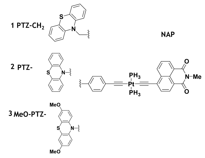
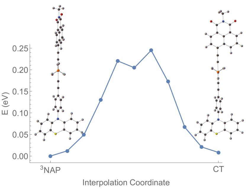
Figure 3: (a.) Chemical structures of the Donor (P), Bridge (-Pt-), Acceptor (NAP) complexes considered here. (b.) Triplet energy along a linear interpolation coordinate connecting the ³NAP minimum energy geometry and the CT minimum energy geometry.

The UV pump-IR push experiments performed on these triads showed that IR-excitation of bridge vibrations after the initial UV pump radically changes the relative yields of the intermediate states. Subsequent excitation of the -CC-Pt-CC- localized vibrations by a timed IR pulse in the CT state of PTZ-complex 2 at 1 ps after the UV pump decreases the yield of the CSS state, whilst increasing that of the ³NAP state. IR-excitation in the course of electron transfer has caused a 100% decrease in the CSS yield in 1, approximately 50% effect in 2, and no effect in 3.

This demonstration of control over excited state dynamics strongly suggests that the acetylide stretching modes are significantly involved in the electron/nuclear coupling in these systems and play central roles in the electron-transfer process. The transferred charge can undergo either further separation to form the full charge-separated state (CSS), or recombine to form a localized excitation, ³NAP. Both eventually decay to ground state. Weinstein et al. showed that if a judiciously chosen IR pump is applied to excite the C$\equiv$C bond after the initial UV excitation, the yield of intermediate states can be radically changed. For example, when a IR pump with frequency = 1,940 $cm^{-1}$ is applied to excite the C$\equiv$C in PTZ-CH₂-Pt-NAP, 1 ps after the UV pump, the yield of the electron transfer state decrease from 32% to 15%, while that of the ³NAP increases from 29% to 46%. The most striking observation is that when a 1,908 $cm^{-1}$ IR pulse is applied to PTZ-CH₂-Pt-NAP 2 ps after UV excitation, the CT $\rightarrow$ CSS step is completely switched off. Delor et al. (2014, 2015); Scattergood et al. (2014).

Quantum chemical analysis indicates that the electron-transfer rate is largely influenced by chemical modification of the PTZ donor. From PTZ-CH₂-Pt-NAP to PTZ-Pt-NAP, to OMe-PTZ-Pt-NAP, the donor strength increases, which increases the energy gap between CT and CSS states. The driving force ($\Delta G$) for the CT $\rightarrow$ CSS transfer also increases from 0.2 eV in PTZ-CH₂-Pt-NAP, to 0.4 eV in PTZ-Pt-NAP, to 0.6 eV in OMe-PTZ-Pt-NAP. Large $\Delta G$ accelerates the CT decay and hence decreases the lifetime of CT state. Comparing PTZ-Pt-NAP and PTZ-CH₂-Pt-NAP, CT transfer to both charge separation and recombination slows down by a factor of about 5 (the lifetime of CT increases from 3.3 to 14 ps and CSS from 190 ps to 1 ns). By appending methoxy groups to the PTZ, the donor strength is increased, and reaction is accelerated. As the result, the lifetime of CT in OMe-PTZ-Pt-NAP is further reduced to 1 ps. Weinstein et al. proposed that the effect of infrared control is caused by the fact that the distance between CT energy minimum and the intersection of CT and CSS potential energy surfaces is small. For all three molecules, two PESs intersect where C$\equiv$C bond is slightly longer than the equilibrium length. When C$\equiv$C bond gets excited, it elongates and helps molecules to pass the intersection. If the energy gap between intersection and equilibrium geometry is much larger than C$\equiv$C vibrational energy, the dynamics is barely affected; if the energy gap is small, the vibrational excitation can radically change the dynamics. Delor et al. (2014, 2015); Scattergood et al. (2014).

III.1 Theoretical Model

We focus our attention on the PTZ system and anticipate that the other systems in this study will exhibit similar behaviour due to the overall similarity of the various donor groups.Yang et al. (ress) For purposes of facilitating the calculations, the molecular structures are simplified such that the P(Bu)₃ moieties and octyl chain of the NAP group were truncated to -PH₃ and a single methyl group, respectively. In all quantum chemical calculations, we used the SDD pseudo-potential for Pt and 6-31G(d, p) for the other atoms. We also used the Polarizable Continuum Model (PCM) to account for the dichloromethane solventas used in Ref.27; 28; 29. The transition dipole moments and electron/hole distributions surfaces were calculated using the Multiwfn (v3.3.8) program.Lu and Chen (2012) An energy level diagram based upon our calculations is sketched in Fig. 4a together with the corresponding electron/hole distribution plots.

	3NAP Geom. (0 eV)		CT Geom. (0.818 eV)
	CSS $\rightarrow$ 3NAP	CT $\rightarrow$ 3NAP	CT $\rightarrow$ 3NAP	CT$\rightarrow$CSS
$\Delta G^{\circ}$ (eV)	0.414	-0.913	-0.781	-0.20
$\lambda$ (eV)	1.01	0.271	1.38	1.08
$V$(eV)	2.56E-4	0.345	1.34E-2	9.22E-3
$\overline{V}$ (eV)	6.34E-2	0.106	0.106	0.192
$\Delta G^{\circ}_{\bar{V}}$ (eV)	0.414	-0.851	-0.770	N/A

Table 1: Driving force $\Delta G^{\circ}$, reorganization energy $\lambda$, diabatic coupling $V$, mean diabatic coupling $\overline{V}$, and $\Delta G^{\circ}_{\bar{V}}$ (driving force calculated with $\overline{V}$), for different transitions

To obtain the diabatic potentials and couplings, we perform a geometry optimization of both the lowest triplet (³NAP) and the third triplet excited states (CT). As discussed below, we use the optimized states as reference geometries for determining the diabatic coupling within the Generalized Mulliken Hush approximation.Cave and Newton (1996, 1997) The normal modes and vibrational frequencies were obtained by harmonic expansion of the energy about the CT state. Once we have determined the diabatic states and couplings, we use the TCLME approach from Ref. Pereverzev and Bittner (2006) to compute the time-correlation functions and state-to-state golden-rule rates as discussed above. We also use the projection technique to determine an optimal set of normal modes and determine the number of such optimal modes that are required to converge the time-correlation functions to a desired degree of accuracy. We then use both the CT and ³NAP minima as reference states for computing the diabatic potentials and couplings necessary for computing rates and modes. Those obtained at the CT minimum can be used to compute transitions originating in from the CT state, while those obtained at the ³NAP minimum can be used for transitions terminating in the ³NAP state.

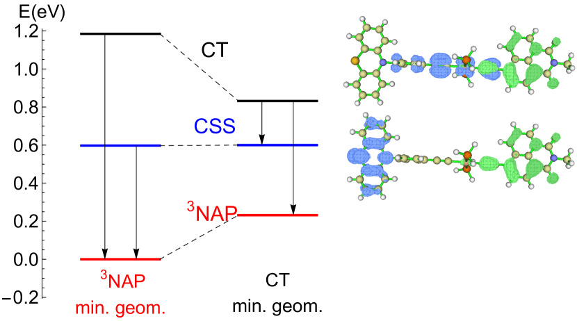
Figure 4: Energy level diagram for the triplet states of PTZ at the ³NAP and CT state geometries. The electron/hole distributions for the CT and CSS are shown to the right (green=electron, blue=hole).

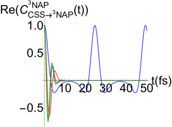
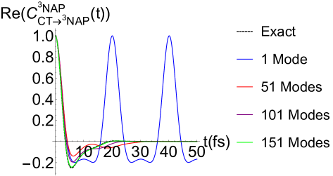
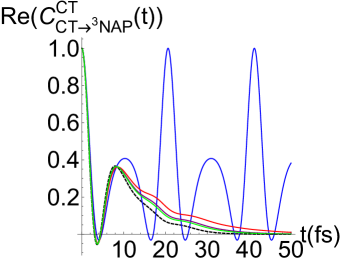
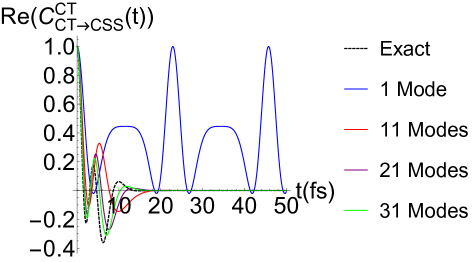
Figure 5: Correlation functions of various numbers of projected modes, compared to exact correlation, for (a) CSS $\rightarrow$ ³NAP at ³NAP geometry, (b) CT $\rightarrow$ ³NAP at ³NAP geometry, (c) CT $\rightarrow$ ³NAP at CT geometry, and (d) CT $\rightarrow$ CSS at CT geometry.

We now compare electron transfer rates as computed using both Marcus theory and the TCLME approach. In the latter case, we examine the convergence of both the time-correlation functions and the rate constants with respect to the number of nuclear modes included in the summation in the construction of the electron-phonon coupling in Eq. 13. For our purposes, an “exact” calculation involves including all nuclear vibrational modes. In our previous work we showed that both $C(t)$ and the total transfer rate constant, $k_{nm}$ calculated using only the first few projected modes provide an excellent agreement with the exact quantities computed using the full set of normal modes, as well as the experimental rates, when parameterized using accurate quantum chemical dataYang and Bittner (2014, 2015).

III.2 Marcus theory rates

The Marcus expression provides a succinct means for the computing transition rates from the driving force $\Delta G^{\circ}$, diabatic coupling $V_{ab}$ and reorganization energy $\lambda$ in Eq. 1. In Table 1, we provide a summary of the parameters computed for the transitions we are considering . The two columns under the heading labeled ³NAP correspond to parameters computed using the ³NAP minimum as a reference geometry while those under the heading labeled CT correspond to parameters computed using the CT reference geometry. The Marcus rates provide a useful benchmark for our approach. Moreover, the parameters in this table portend a difficulty in using the ³NAP geometry as a reference. For example, for the CSS $\rightarrow^{3}$NAP transition, the driving force is in the wrong direction since it predicts that the CSS state lies lower in energy than the ³NAP state, which is inconsistent with both experimental observations and our quantum chemical analysis in Figure 4.

	CT Geom.		3NAP Geom.
Rates (ps-1)	CT$\to$ CSS	CT $\to^{3}$NAP	CT $\to^{3}$NAP	CSS$\to^{3}$NAP
Exp.	0.0879	0.097	0.097	1.84E-3
Marcus	0.846	0.2043	1002.82	8.250E-11
Marcus (Mean V)	365.7	12.75	95.23	5.04E-6
TCLME	0.725	0.0562	12.89	3.022E-8
TCLME + PLM	0.627	0.0488	21.6	0.500E-4
TCLME (Mean V)	–	2.79	8.931	1.51E-3

Table 2: Comparison between experimental and computed state to state transition rates for PTZ. The experimental rates for each process are obtained from Ref. 28.

III.3 TCLME Rates

To compute the rates using the TCLME expression (Eq. 24), we begin by computing the electron/nuclear correlation function and compare its convergence with respect to the number of Lanczos modes. Recall that the Lanczos modes are determined by an iterative ranking algorithm that identifies superpositions of normal modes that optimize the electron/phonon coupling. Fig. 5 gives a summary of these numerical tests in which we compute $C_{nm}(t)$ vs. time with an increasing number of Lanczos modes. In all cases, we compare to the “exact” result in which all nuclear modes were used. The top two figures (Fig. 5a and b) use the ³NAP as the reference geometry. In these cases, convergence of $C_{nm}(t)$ with respect to the number of modes proved to be problematic for both transitions considered. Correspondingly, the rates computed using this geometry also compare poorly against the observed experimental rates, although are an order of magnitude closer than Marcus rates. We speculate that this may signal a break-down in the Condon approximation which insures separability between nuclear and electronic degrees of freedom.

In Table 2, we summarize both the experimental and computed state to state rates for the PTZ system. Given the complexity and size of the system, overall the numerical rates computed using the exact TCLME approach are in quantitative agreement with the experimental rates, particularly for those using the CT geometry as a reference point (cf Fig. 5c and d). We note that fewer projected modes (30-50) are needed to converge the correlation function out to the first 50 fs when using the CT-geometry. Furthermore, while Marcus rate for the CT$\to$ CSS transition agrees with the exact TCLME result, it misses the CT $\to^{3}$NAP experimental rate by 4 orders of magnitude whereas the TCLME rate is in much better agreement with the experimental rate.

If we compare the exact TCLME rate, which uses the full set of normal modes in constructing the $C_{nm}(t)$ correlation function, to the rate computed used only the PLM (TCLME+PLM), for both the CT$\to$ CSS and CT $\to^{3}$NAP rates, the single mode approximation is within 86% of the exact result. This indicates that while multiple vibrational normal modes contribute to the electronic coupling, the linear combination identified by the projection algorithm carries the vast majority of the electron/phonon coupling. This is consistent with our previous study of triplet energy transfer in small donor-bridge-acceptor systems. Yang and Bittner (2014, 2015)

III.4 Primary Mode Approximation

As discussed earlier, our ranking algorithm allows us to rapidly determine the vibrational motions that optimize the electron/nuclear couplings. In addition to providing an accurate way to compute rate constants, they provide additional insight into actual dynamics. Here, we shall focus upon the transitions originating from the CT geometry. Generally speaking, the highest ranked mode, termed the “Primary Lanczos Mode” (PLM), captures much of the short-time dynamics of the transitions. In Fig. 5, we show the electronic coupling correlation functions computed using different numbers of projected modes for all four transitions. For the CT $\rightarrow$ ³NAP transition, the primary mode resembles the exact initial dynamics for the first 10 fs and roughly 10 or so modes are sufficient to converge the correlation function out to times longer than the correlation time. In Table 2 we see that for the CT geometry, the primary mode approximation is sufficient to obtain accurate rate constants. On the contrary, it takes considerably more modes modes to recover the full correlation function for transition originating from the ³NAP geometry.

Fig. 6(a-d) shows the projection of the primary mode identified for each transition onto the normal vibrational modes of the originating state, i. e., the primary modes calculated at CT geometry are projected onto the normal modes of the CT state, and those at the ³NAP geometry are projected onto the normal modes of the ³NAP state. In all four cases, the primary mode is dominated by symmetric and anti-symmetric contributions from the C$\equiv$C displacements. While both transitions involve acetylene bond-stretching motions, the CT$\to$CSS transition involves only the symmetric combination, whereas the CT$\to^{3}$NAP involves both the symmetric and anti-asymmetric combination. It is tempting to conclude from this that that the secondary IR push used in the experiments preferentially excites the anti-symmetric mode and thus selectively enhances the CT$\to^{3}$NAP transition. In fact, the computed IR oscillator strength of the anti-symmetric mode is an order of magnitude greater than the symmetric mode. Similarly, from experiment, the anti-symmetric normal mode extinction coefficient is 3 times larger than that for the symmetric normal mode. However, the time-scale for the IR excitation is sufficient long enough that both symmetric and anti-symmetric CC modes are expected to be equally populated by the IR push pulse.

In the CT$\to^{3}$NAP transition, both types of acetylene stretching motions (symmetric and anti-symmetric) contribute more or less equally to the electronic coupling while in the CT$\to$CSS transition, only the symmetric acetylene motion carries the majority of the coupling. This mechanism can be rationalized by the way the vibrational populations enter into our expression for electron/nuclear coupling correlation function in Eq. 17. In principle, the expression was derived assuming a thermal population of the vibrational modes. However, if we assume that the role of the IR pulse is to excite the $C\equiv C$ stretching modes by one vibrational quantum, then the value of $\bar{n}_{i}$ appearing in Eq.  17 for those modes should be increased to $\bar{n}_{i}+1$. Consequently, driving these modes with the IR pulse increases the total electronic coupling, consistent with the experimental observation that IR excitation following formation of the CT states accelerates the CT$\to^{3}$NAP transition relative to the CT$\to$CSS transition.

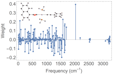
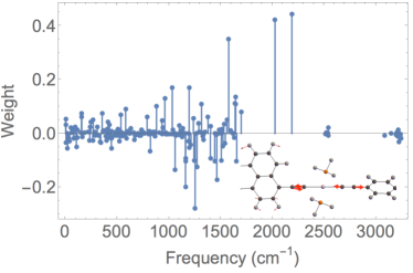
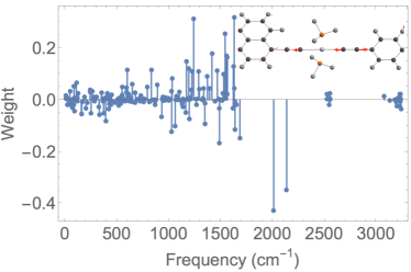
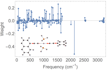
Figure 6: Component projection of the primary mode onto the normal modes for the following transitions: (a) CSS $\rightarrow$ ³NAP, (b) CT $\rightarrow$ ³NAP calculated at ³NAP geometry. (c)CT $\rightarrow$ ³NAP, and (d) CT $\rightarrow$ CSS calculated at CT geometry. Embedded molecule shows the atomic displacement vectors of primary mode.

IV Discussion

We here a review of our work in developing new tools for analysing electronic transitions in complex molecular systems. Central to our work is the notion that one can systematically identify a subset of vibrational modes that capture the majority of the electronic coupling to the nuclear motions. These primary modes capture the short-time dynamics with sufficient accuracy for computing the salient correlation and response functions necessary for evaluating the golden-rule rates for state-to-state transitions. While not a central theme to this review, our time-convolutionless master equation method can be used for computing multi-state transitions and in cases where the state to state rates are time-dependent. Tamura et al. (2008); Pereverzev et al. (2009)

We believe that the key to understanding and ultimately controlling electron transfer pathways in a complex molecular species is through vibronic coupling. The approach we have delineated in this article offers a systematic way to deduce a subset of nuclear motions that are most responsible for driving electronic transitions. When paired with the TCLME approach for computing the state-to-state transitions, we can obtain rate constants that are in quantitative agreement with experimental rates and probe deeper into the dynamics to understand which specific types of nuclear motions are involved in a given transition. The algorithm illustrated here in the example of photo-induced charge-transfer should be of considerable utility for understanding of a multitude of light-induced reactions where several electronic states are involved in ultrafast transformations.

References

- Marcus (1956) R. A. Marcus, The Journal of Chemical Physics 24, 966 (1956).
- Marcus (1965) R. A. Marcus, The Journal of Chemical Physics 43, 679 (1965).
- Marcus (1993) R. A. Marcus, Reviews of Modern Physics 65, 599 (1993).
- Miller et al. (1984) J. Miller, L. Calcaterra, and G. Closs, Journal of the American Chemical Society 106, 3047 (1984).
- Pereverzev and Bittner (2006) A. Pereverzev and E. R. Bittner, The Journal of Chemical Physics 125, 104906 (2006).
- Tamura et al. (2008) H. Tamura, J. G. Ramon, E. R. Bittner, and I. Burghardt, Physical Review Letters 100, 107402 (2008).
- Tamura et al. (2007) H. Tamura, E. R. Bittner, and I. Burghardt, The Journal of Chemical Physics 126, 021103 (2007).
- Bittner and Silva (2014) E. R. Bittner and C. Silva, Nature Communications 5 (2014).
- Singh et al. (2009) J. Singh, E. R. Bittner, D. Beljonne, and G. D. Scholes, The Journal of Chemical Physics 131, 194905 (2009).
- Cederbaum et al. (2005) L. S. Cederbaum, E. Gindensperger, and I. Burghardt, Physical Review Letters 94, 113003 (2005).
- Gindensperger et al. (2006a) E. Gindensperger, I. Burghardt, and L. S. Cederbaum, The Journal of Chemical Physics 124, 144103 (2006a).
- Gindensperger et al. (2006b) E. Gindensperger, I. Burghardt, and L. S. Cederbaum, The Journal of Chemical Physics 124, 144104 (2006b).
- Pereverzev et al. (2009) A. Pereverzev, E. R. Bittner, and I. Burghardt, The Journal of Chemical Physics 131, 034104 (2009).
- Subotnik et al. (2008) J. E. Subotnik, S. Yeganeh, R. J. Cave, and M. A. Ratner, The Journal of Chemical Physics 129, 244101 (2008).
- Subotnik et al. (2009) J. E. Subotnik, R. J. Cave, R. P. Steele, and N. Shenvi, The Journal of Chemical Physics 130, 234102 (2009).
- Subotnik et al. (2010) J. E. Subotnik, J. Vura-Weis, A. J. Sodt, and M. A. Ratner, The Journal of Physical Chemistry A 114, 8665 (2010).
- Grover and Silbey (1970) M. K. Grover and R. Silbey, The Journal of Chemical Physics 52, 2099 (1970).
- Rice and Gartstein (1994) M. Rice and Y. N. Gartstein, Physical Review Letters 73, 2504 (1994).
- Edmiston and Ruedenberg (1963) C. Edmiston and K. Ruedenberg, Reviews of Modern Physics 35, 457 (1963).
- Domcke et al. (2004) W. Domcke, D. R. Yarkony, and H. Köppel, Conical Intersections: Electronic structure, Dynamics and Spectroscopy, Advanced Series in Physical Chemistry, Vol. 15 (World Scientific Co., 2004).
- Mead and Truhlar (1982) C. A. Mead and D. G. Truhlar, The Journal of Chemical Physics 77, 6090 (1982).
- Yang and Bittner (2014) X. Yang and E. R. Bittner, The Journal of Physical Chemistry A 118, 5196 (2014).
- Yang and Bittner (2015) X. Yang and E. R. Bittner, The Journal of Chemical Physics 142, 244114 (2015).
- Cave and Newton (1996) R. J. Cave and M. D. Newton, Chemical Physics Letters 249, 15 (1996).
- Cave and Newton (1997) R. J. Cave and M. D. Newton, The Journal of Chemical Physics 106, 9213 (1997).
- Yang et al. (ress) X. Yang, T. Keane, M. Delor, A. J. H. M. Meijer, J. Weinstein, and E. R. Bittner., Nature Communications (in press).
- Delor et al. (2014) M. Delor, P. A. Scattergood, I. V. Sazanovich, A. W. Parker, G. M. Greetham, A. J. Meijer, M. Towrie, and J. A. Weinstein, Science 346, 1492 (2014).
- Delor et al. (2015) M. Delor, T. Keane, P. A. Scattergood, I. V. Sazanovich, G. M. Greetham, M. Towrie, A. J. Meijer, and J. A. Weinstein, Nature Chemistry (2015).
- Scattergood et al. (2014) P. A. Scattergood, M. Delor, I. V. Sazanovich, O. V. Bouganov, S. A. Tikhomirov, A. S. Stasheuski, A. W. Parker, G. M. Greetham, M. Towrie, E. S. Davies, et al., Dalton Transactions 43, 17677 (2014).
- Lu and Chen (2012) T. Lu and F. Chen, Journal of Computational Chemistry 33, 580 (2012).