TIMING ANALYSIS IN MICROLENSING

Abstract

Timing analysis is a powerful tool used to determine periodic features of physical phenomena. Here we review two applications of timing analysis to gravitational microlensing events. The first one, in particular cases, allows the estimation of the orbital period of binary lenses, which in turn enables the breaking of degeneracies. The second one is a method to measure the rotation period of the lensed star by observing signatures due to stellar spots on its surface.

PACS numbers: 95.75De, 97.10.Qh

1 Introduction

The timing analysis is the study of a repetitive feature of a phenomenon in order to investigate its dynamic properties and infer its period. Timing analysis has always been a key tool for the search and the study of exoplanets. For example, the radial velocity method is based on timing analysis of the velocity profile along the line of sight of the parent star. The transit method relies on the periodic repetition of a same feature, the dimming of the light of a star produced by the passing of a planet over the star’s disk. Furthermore, cold and hotspots are generally present on the star surface, and if a starspot is observed in different transits, it is possible to assess the rotation period and velocity of the star, the sky-projected orbital obliquity of the planetary system, and, in some cases, the true orbital obliquity.[1]

Small variations from a perfectly periodic behavior give often hints about the presence of perturbations that can reveal new phenomena. For example, the first exoplanets, around the pulsar PSR B1257+12, were discovered through the detection of anomalies in the spin period of the neutron star.[2] It has been proposed[3, 4, 5] to perform timing analysis of transit times in order to find deviations from the linear ephemeris (TTV, Timing Transit Variations), likely due to the presence of an unknown body, as a moon or a planet.[6] This method has been used, for example, to confirm and characterize the planet Kepler-9 d[7].

Gravitational microlensing is an inefficient method to find new planets with respect to transit and radial velocity methods, as a consequence of its low optical depth, of the order of $10^{-7}$ in the most favorable situations. Yet, this technique, which is in some sense complementary to the other methods, is the only able to detect very distant exoplanets in the Galactic Bulge or outer galaxies[8, 9] and leads to a complete characterization of the these systems. Its use brought important discoveries in the field of exoplanets, like the facts that cold Neptunes[10], free-floating planets,[11] and terrestrial planets in low-mass binaries[12] are more common than previously expected. Differently from most of the other methods to detect exoplanets, microlensing offers generally a single non-repeatable event (except for self-lensing events, like KOI-3278[13]). Nonetheless, periodic deviations from the standard microlensing amplification curves may give some information on the lensing system or the source star.

We consider here two applications of timing analysis in the context of gravitational microlensing. The first one, discussed in Section 2, allows us to estimate, with some caveats, the orbital period of the binary lens.[14] The second application, outlined in Section 3, is about the determination of rotating period of the source star thanks to the presence of stellar spots on its surface.[15]

2 Rotating Binaries

The discovery of exoplanets by microlensing is made possible by the fact that the presence of a companion of the main lensing object induces deviations from the standard Paczyński curve which characterizes a single lens event.[16]

In order to fit the amplification curve due to a binary lens system a number of parameters has to be taken into account. Four parameters are those used to model a single lens event: $u_{0}$, the distance of closest approach between the lens and the source projected in the sky; the time $t_{0}$ of closest approach; the Einstein time $t_{\textup{E}}$; the angle $\theta$ of the source’s trajectory in the plane of the lens. Further parameters are the projected separation $s$ between the lenses, and their mass ratio $q=m_{2}/m_{1}$, being $m_{1}$ and $m_{2}$ the masses of the two lenses. If the background source is not point-like, finite size effects should be taken into account by considering the source radius $\rho_{*}$ as well. Furthermore, if the orbital motion of the lenses is not negligible, six additional parameters are required to model the event: the semi-major axis $a$ (that is related to the lenses sepration $s$), the orbital eccentricity $e$, the time of passage at periapsis $t_{\textup{p}}$, the inclination angle $i$ between the normal to the lens orbital plane and the line of sight, the orientation $\varphi$ of the orbital plane in the sky, and the orbiting versus (either clockwise or counterclockwise). This is only one of the possible sets of parameters that can be used to describe such events. Furthermore, there are some degeneracies that may add complexity to this scheme. For example, under certain circumstances the caustics resulting from two lenses separated by a projected distance $s$ or $1/s$ have the same structure, implying that the observed light curves will appear the same. This is the so called close-wide degeneracy that may occur in lensing systems with $q\ll 1$, like in planetary systems.[17]

The modeling of a microlensing event by binary lenses can be a daunting task, due to the large parameter space to be explored, and could take several CPU hours. One of the most delicate aspects of a fitting procedure, that can speed up the convergence to the best solution, is the choice of good starting values, as close as possible to the true ones. Most of the parameters of a Paczyński curve are often easy to estimate by eye looking to the amplification curve: $t_{\textup{E}}$ is the timescale of the event, the half-width of the curve is roughly $t_{\textup{E}}$; $t_{0}$ is the position of the main peak of the curve; the asymptotic behavior of the amplification $A$ for small values of the distance of closest approach is[18] $A\sim 1/u_{0}$, so that $u_{0}$ can be readily guessed by measuring the amplification of the main peak. It has been argued[19] that also other parameters of a binary lens event can be estimated by eye in some cases, but not all.

We also mention that also the source may be in a binary system, even if binary sources have been seldom recognized in photometric microlensing observations. In this respect, a more efficient method for the detection of their orbital motion is given by astrometric microlensing.[18]

2.1 Estimating the orbital period

The orbital period $P$ of a binary lensing system is related to its semi-major axis $a$ by the Kepler’s third law:

$$P=2\pi\sqrt{\frac{a^{3}}{Gm_{1}(1+q)}}$$ (1)

Thus, measuring the orbital period $P$ of the lensing system by means of timing analysis, independently from a fit to the microlensing amplification curve, could give a quantity that is important by itself and help in better constraining some of the free parameters of the full fit of the amplification curve.

The method we first proposed in Ref. 2014MNRAS.438.2466N consists in searching for the amplification curve by a single lens that fits best the amplification curve by the binary lens under examination, which shows non-negligible effects of the lens orbital motion. Of course, this method can be applied only when the shape of this curve closely resembles that of a Paczyński curve. The residuals between the two curves present periodic features that allow the estimation of the orbital period of the binary lensing system by using timing analysis. This procedure removes the underlying trend and lets the periodic features of the curve emerge. This is a simple task to perform because the parameters of a Paczyński curve can be easily guessed, as discussed above. Another limitation is that, in order to be able to apply the timing analysis, the orbital period of the lenses should be shorter than the Einstein time of the event, or we must have a long observational window so that the lenses complete at least two orbits during the observations. In addition, care must be used when analyzing the results, because this procedure may give half of the true period, even though the order of magnitude is correctly retrieved.

2.2 Simulations of binary lens events

We tested this method by performing simulations of microlensing events involving binary lenses with relevant orbital motion during the event. There are different techniques to calculate the amplification by binary lenses, each one with its advantages and drawbacks. Some of these techniques are:

• Witt & Mao method:[20] these authors showed that, if the source is far enough from the caustic, the amplification of a point-like source by binary lenses can be computed by solving a fifth-order polynomial with complex coefficients. This method is fairly fast, the major bottleneck being the search of the roots of the polynomial,[21] but the restriction on the position of the source (far enough from the caustic) limits its application.

• Hexadecapole method:[22] this method enables the calculation of the amplification of an extended source and stems from the fourth-order Taylor expansion of this quantity. It consists in measuring the amplification of a point-like source in thirteen positions. For the amplification by binary lenses the Witt & Mao method can be employed to compute these amplifications of a point-like source. This method is fast, is designed for extended sources, works with any lens configuration and takes into account the limb-darkening effect as well, but can be applied far enough from the caustic (but generally closer than the Witt & Mao method).

• Inverse ray shooting:[23, 24] it consists in “shooting” a large number of “photons” from the observer towards the source star and apply the lens equation[16] to compute the deflection by the lenses. This method is accurate and works with extended source and any lens configuration, even when the source crosses the caustic, the locus of the points in the lens plane where the amplification diverges to infinity. On the other hand, this technique is also computationally costly, especially in the case of lens orbital motion.

We adopted a hybrid approach, using all techniques but each one only where necessary, in order to take the best of all methods and speed up calculations. In particular, we decided to use the inverse ray shooting method when the source is close to the caustics, and the hexadecapole method combined with the Witt & Mao amplification when the source is far enough from the caustic. We address the reader to Ref. 2014MNRAS.438.2466N for details.

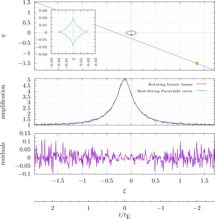
Figure 1: Upper panel: Geometry of the microlensing event. Purple straight line represents the trajectory of the source (the yellow dot on bottom right) in the lens plane $\xi-\eta$, from bottom right to top left. The small green and yellow elliptical curves around the origin are the orbits of the lenses. The inset on the left shows a zoom in of the central caustic of the lenses, at the end of the simulation. Middle panel: Amplification of the source by the rotating binary lenses ($A_{\textup{BL}}$) and its best-fitting Paczyński model ($A_{\textup{SL}}$). Gaussian noise has been added to the simulated amplification $A_{\textup{BL}}$. Lower panel: residuals $(A_{\textup{BL}}-A_{\textup{SL}})/A_{\textup{SL}}$ of the amplification curve by rotating binary lenses relative to the Paczyński model. Note these are not the absolute residuals, that would be $A_{\textup{BL}}-A_{\textup{SL}}$.

Here we present a new simulation of a microlensing with rotating binary lenses. We adopted dimensionless quantities, with lengths expressed in units of the Einstein radius $R_{\textup{E}}$ and times in units of the Einstein time $t_{\textup{E}}$.[14] The source star has radius $\rho_{*}=0.03$, limb-darkening coefficient $\Gamma=0.5$, and its projected distance of closest approach to the center of mass of the lenses is $u_{0}=0.2$. The lenses have mass ratio $q=0.9$, their orbit has semi-major axis $a=0.2$, eccentricity $e=0$, and period $P=0.4$. Inclination angle $i$ and rotation $\phi$ are both set to $0$. The geometry of the system and the results of the simulations are shown in Fig. 1.

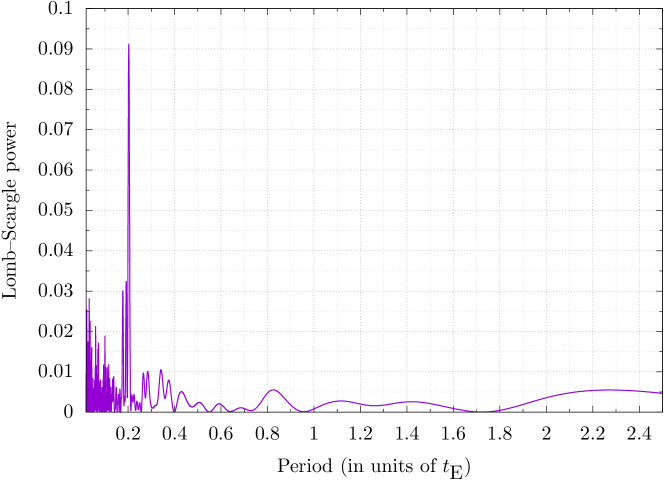
Figure 2: Lomb–Scargle periodogram of the residuals in Fig. 1. We adopted the standard normalization, suggested by Refs. 1976Ap&SS..39..447L,2009AA…496..577Z, for which the Lomb–Scargle power $p(P)$ is in the range $[0,1]$, standing $p(P)=0$ for no periodicity in the data with period $P$, and $p(P)=1$ for a “perfect” periodicity with period $P$.

We then applied the generalized Lomb–Scargle periodogram[27] to the relative residuals shown in Fig. 1, using the LombScargle.jl package written in Julia language. We found that spurious peaks in the residuals appears within the central part of the event,[14] so we had to remove a small region around $t=0$ before actually performing the periodogram. The result of this timing analysis is shown in Fig. 2. The period with the highest peak is $P=0.203$, which is half of the simulated orbital period $P=0.4$ of the lenses, because the caustic is symmetric[14] (see inset of Fig. 1). In Ref. 2014MNRAS.438.2466N are presented cases where the caustic is not symmetric and the correct period is found.

3 Starspots on Rotating Source Star

Many authors suggested to exploit microlensing events in order to study irregularities on the surface of the source star, like cold- and hotspots, either with photometric[28, 29, 30, 31] or polarimetric microlensing observations.[32] This effect is particularly important since the presence of stellar spots on the source may fake planetary features in events that are actually due to a single lens, as occurred in the case of MOA-2010-BLG-523.[33] However, none of the above mentioned works took into account the possibility for the source star and/or the binary lens system to rotate. We filled this gap in Ref. 2015MNRAS.453.2017G and showed that also in this case timing analysis could be a powerful tool to get more information on the considered system.

3.1 Application of timing analysis

In a manner similar to the one described in Section 2.1, we will show that by applying timing analysis to the residuals of a fit of a “static” curve to an intrinsically periodic curve we can retrieve the rotating period of the lensed star.

In Ref. 2015MNRAS.453.2017G we performed simulations of microlensing events with single and binary lenses, involving a rotating source and/or rotating lenses. The amplification $A_{\textup{s}}$ of the spotted star has been calculated as the weighted average of the amplification $A(\vec{r})$ over the star disc $\mathcal{S}$, using as weight the surface brightness $f(\vec{r})$

$$A_{\textup{s}}=\frac{\int_{\mathcal{S}}A(\vec{r})f(\vec{r})\mathrm{d}^{2}\vec{r}}{\int_{\mathcal{S}}f(\vec{r})\mathrm{d}^{2}\vec{r}}.$$ (2)

The amplification $A(\vec{r})$ is the amplification of a point-like source by either a single or a binary lens, depending on the event. Also in this work we employed a hybrid approach for calculating the amplification by a binary lens, like the one discussed in Section 2.2, using inverse ray shooting when the source is close to the caustic, and Witt & Mao method far enough from the caustic. The surface brightness profile $f(\vec{r})$ is defined as

$$f(\vec{r})=\begin{cases}l(\vec{r})&\text{outside the spot}\\ c~{}l(\vec{r})&\text{inside the spot},\end{cases}$$ (3)

where $l(\vec{r})$ is the brightness of the unspotted star, and $c$ is the contrast parameter, that is the ratio between the brightness of the spot and the unspotted surface. The case $c>1$ corresponds to hotspots, $c<1$ is for coldspots.

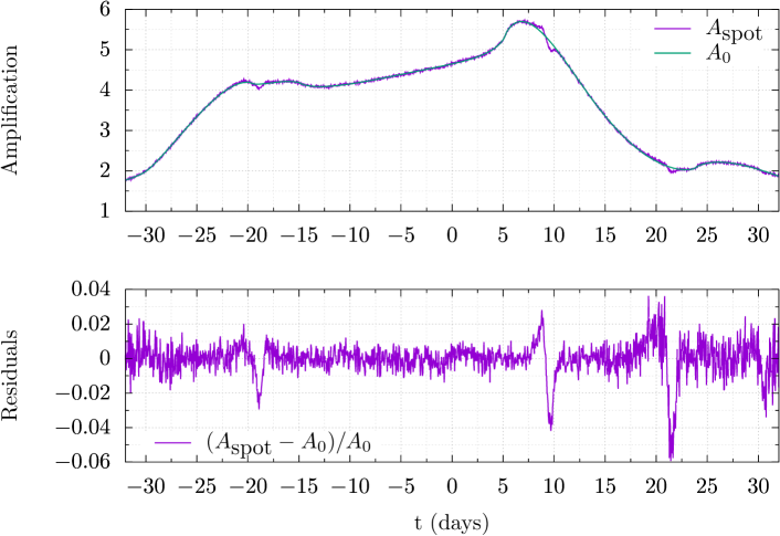
Figure 3: Results of the simulation described in the text. Upper panel: amplification curve of the unspotted star ($A_{0}$) and the spotted one ($A_{\textup{spot}}$). Gaussian noise has been added to the amplification $A_{\textup{spot}}$ of the spotted star. Lower panel: the residuals $(A_{\textup{spot}}-A_{0})/A_{0}$ of the spotted star model relative to the unspotted one are represented. Note these are not the absolute residuals, that would be $A_{\textup{spot}}-A_{0}$.

Here we present a new simulation of a microlensing event of a rotating star by a static binary lens. The lens system is constituted by two equal mass objects, so their mass ratio is $q=1$, and they are at a projected separation of $b=1$. The ratio $D_{\textup{l}}/D_{\textup{s}}$ between the observer-lens distance $D_{\textup{l}}$ and observer-source distance $D_{\textup{s}}$ is equal to $0.5$. The source star has rotation period $P=10~{}\mathrm{d}$, typical of main-sequence G2 stars observed by Kepler,[34] and its projected radius is $\rho_{*}=0.1$. The limb-darkening coefficient adopted in the simulation is $\Gamma=0.45$. We considered both a star with a spot on its surface and a star without any such feature. Starspots can have a variety of sizes, covering up to $22\%$ of the stellar hemisphere.[35] We simulated a coldspot with center on the equator (corresponding to colatitude $\theta=\pi/2$), contrast $c=0.1$, and radius equal to $0.2~{}\rho_{*}$. In Fig. 3 the results of the simulations are shown.

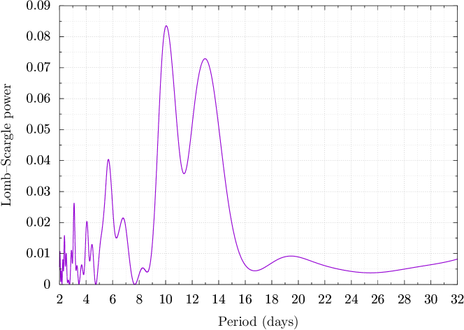
Figure 4: Lomb–Scargle periodogram of the residuals in Fig. 3. It has the same standard normalization used in for the periodogram in Fig. 2. The simulation spans 64 days, therefore the largest period we consider in the periodogram is 32 days, the half width of the time series.

We applied the generalized Lomb–Scargle periodogram to the absolute value of the relative residuals shown in Fig. 3, using the fast algorithm[36] provided by the LombScargle.jl package. In Fig. 4 the periodogram is shown. The period with the largest power is $P_{1}=10.05~{}\mathrm{d}$. Another peak is present at $P_{2}=12.97~{}\mathrm{d}$, but while the highest peak at $P_{1}$ is replicated by a broad peak at the higher harmonic $P=19.44~{}\mathrm{d}$, there is no higher harmonic peak for the secondary peak at $P_{2}$, suggesting that the period at $P_{1}$ is the real one, which is indeed very close to the rotation period $P=10~{}\mathrm{d}$ of the source star we used in the simulation. Thus, in this case we showed that the application of the timing analysis to the residuals allows us to measure the rotation period of the source star.

4 Comments

In this paper we considered two possible applications of timing analysis to gravitational microlensing events. In both cases, the use of this tool enabled us to recover important information about the simulated system.

In Section 2 we showed that even applying an inappropriate fitting function to the amplification curve can be useful. We fitted a microlensing event due to a rotating binary with the Paczyński model, with the mere purpose of enhancing the periodic features through a sort of detrending procedure. Using the Lomb–Scargle periodogram with the residuals, we were able to find half of the true orbital period of the binary lensing system with good accuracy. Nevertheless, the knowledge of at least the order of magnitude of the orbital period makes it possible to better constrain some of the free parameters of the real fit to the observed curve.

The presence of spots on the surface of the star induces small deviations from the standard amplification curve. In Section 3 we have been able to get the rotation period of the star by measuring the residuals of the amplification of the spotted star relative to the amplification of the unspotted star, and then applying the Lomb–Scargle periodogram on them. The analysis of spot features requires high-precision and high-cadence photometry, because these signatures can last a few hours. The Korean Microlensing Telescope Network (KMTNet) can collect up to 6 data points per hour[37] and could be able to observe starspots features. By using observational parameters of OGLE-III and OGLE-IV campaigns, we estimated in Ref. 2015MNRAS.453.2017G the number of events with these features to be about $4.7$ per year towards the Galactic Bulge.

References

- [1] J. Southworth and L. Mancini, ArXiv e-prints (August 2016) arXiv:1608.03095 [astro-ph.EP].
- [2] A. Wolszczan and D. A. Frail, Nature 355 (January 1992) 145.
- [3] J. Miralda-Escudé, ApJ 564 (January 2002) 1019, astro-ph/0104034.
- [4] M. J. Holman and N. W. Murray, Science 307 (February 2005) 1288, astro-ph/0412028.
- [5] E. Agol, J. Steffen, R. Sari and W. Clarkson, MNRAS 359 (May 2005) 567, astro-ph/0412032.
- [6] D. M. Kipping, MNRAS 392 (January 2009) 181, arXiv:0810.2243.
- [7] M. J. Holman, D. C. Fabrycky, D. Ragozzine, E. B. Ford et al., Science 330 (October 2010) 51.
- [8] S. Calchi Novati, G. Covone, F. de Paolis, M. Dominik, Y. Giraud-Héraud, G. Ingrosso, P. Jetzer, L. Mancini, A. Nucita, G. Scarpetta, F. Strafella and A. Gould, A&A 469 (July 2007) 115, arXiv:0704.1408.
- [9] G. Ingrosso, S. C. Novati, F. de Paolis, P. Jetzer, A. A. Nucita and A. F. Zakharov, MNRAS 399 (October 2009) 219, arXiv:0906.1050 [astro-ph.SR].
- [10] A. Gould, A. Udalski, D. An, D. P. Bennett et al., ApJL 644 (June 2006) L37, astro-ph/0603276.
- [11] T. Sumi, K. Kamiya, D. P. Bennett, I. A. Bond et al., Nature 473 (May 2011) 349, arXiv:1105.3544 [astro-ph.EP].
- [12] A. Udalski, Y. K. Jung, C. Han, A. Gould et al., ApJ 812 (October 2015) 47, arXiv:1507.02388 [astro-ph.EP].
- [13] E. Kruse and E. Agol, Science 344 (April 2014) 275, arXiv:1404.4379 [astro-ph.SR].
- [14] A. A. Nucita, M. Giordano, F. De Paolis and G. Ingrosso, MNRAS 438 (March 2014) 2466, arXiv:1401.6288 [astro-ph.SR].
- [15] M. Giordano, A. A. Nucita, F. De Paolis and G. Ingrosso, MNRAS 453 (October 2015) 2017, arXiv:1508.04340 [astro-ph.SR].
- [16] F. De Paolis, M. Giordano, G. Ingrosso, L. Manni, A. Nucita and F. Strafella, Universe 2 (March 2016) 6, arXiv:1604.06601.
- [17] K. Griest and N. Safizadeh, ApJ 500 (June 1998) 37, astro-ph/9710342.
- [18] A. A. Nucita, F. De Paolis, G. Ingrosso, M. Giordano and L. Manni, ApJ 823 (June 2016) 120, arXiv:1606.02062 [astro-ph.SR].
- [19] A. Gould and A. Loeb, ApJ 396 (September 1992) 104.
- [20] H. J. Witt and S. Mao, ApJL 447 (July 1995) L105.
- [21] V. Bozza, MNRAS 408 (November 2010) 2188, arXiv:1004.2796 [astro-ph.EP].
- [22] A. Gould, ApJ 681 (July 2008) 1593, arXiv:0801.2578.
- [23] P. Schneider and A. Weiß, A&A 164 (August 1986) 237.
- [24] R. Kayser, S. Refsdal and R. Stabell, A&A 166 (September 1986) 36.
- [25] J. Skowron and A. Gould, ArXiv e-prints (March 2012) arXiv:1203.1034 [astro-ph.EP].
- [26] N. R. Lomb, Ap&SS 39 (February 1976) 447.
- [27] M. Zechmeister and M. Kürster, A&A 496 (March 2009) 577, arXiv:0901.2573 [astro-ph.IM].
- [28] D. Heyrovský and D. Sasselov, ApJ 529 (January 2000) 69, astro-ph/9906024.
- [29] C. Han, S.-H. Park, H.-I. Kim and K. Chang, MNRAS 316 (August 2000) 665, astro-ph/0001490.
- [30] H.-Y. Chang and C. Han, MNRAS 335 (September 2002) 195, astro-ph/0201121.
- [31] M. A. Hendry, H. M. Bryce and D. Valls-Gabaud, MNRAS 335 (September 2002) 539, astro-ph/0210208.
- [32] S. Sajadian, MNRAS 452 (September 2015) 2587, arXiv:1506.08359 [astro-ph.SR].
- [33] A. Gould, J. C. Yee, I. A. Bond et al., ApJ 763 (February 2013) 141, arXiv:1210.6045 [astro-ph.SR].
- [34] M. B. Nielsen, L. Gizon, H. Schunker and C. Karoff, A&A 557 (September 2013) L10, arXiv:1305.5721 [astro-ph.SR].
- [35] K. G. Strassmeier, The Astronomy and Astrophysics Review 17 (September 2009) 251.
- [36] W. H. Press and G. B. Rybicki, ApJ 338 (March 1989) 277.
- [37] C. B. Henderson, B. S. Gaudi, C. Han, J. Skowron, M. T. Penny, D. Nataf and A. P. Gould, ApJ 794 (October 2014) 52, arXiv:1406.2316 [astro-ph.EP].