$E_{6}$ Yukawa couplings in F-theory
as D-brane instanton effects

Abstract

In a weak coupling limit the neighborhood of $E_{6}$ Yukawa points in $SU(5)$ GUT F-theory models is described by a non-resolvable orientifold of the conifold. We explicitly show, first directly in IIB and then via a mirror symmetry argument, that in this limit the $E_{6}$ Yukawa coupling is better described as coming from the non-perturbative contribution of a euclidean D1-brane wrapping the non-resolvable cycle. We also discuss how the M-theory description interpolates between the weak and strong coupling viewpoints.

1 Introduction

In recent years, starting with Donagi:2008ca ; Beasley:2008dc ; Hayashi:2008ba ; Beasley:2008kw ; Donagi:2008kj , F-theory Vafa:1996xn has emerged as a rich and powerful framework in which to do string model building, and more specifically GUT model building. The main desirable feature that distinguishes F-theory from ordinary type IIB model building at weak coupling is the natural appearance of the $\bf 10\,\bf 10\,\bf 5$ Yukawa coupling in $SU(5)$ GUT F-theory models, which in weakly coupled IIB models can only realized via D-brane instanton effects, i.e. nonperturbatively, and is thus expected to be fairly suppressed. Since phenomenological constraints require the $\bf 10\,\bf 10\,\bf 5$ coupling associated to the top quark multiplet to be of order one, a non-perturbative suppression factor makes realistic model building in IIB a challenge. The situation in F-theory seems to be better, with computations of the physical Yukawa couplings in toy models yielding promising results Font:2012wq ; Font:2013ida ; Marchesano:2015dfa ; Carta:2015eoh . To a large extent this feature of F-theory justifies the considerable effort spent in developing the theoretical tools behind F-theory model building in the last few years, trying to address the significantly increased technical difficulties involved in computing important physical aspects of the backgrounds (when compared to the weakly coupled IIB approach), such as quantum corrections to Kähler potentials GarciaEtxebarria:2012zm ; Minasian:2015bxa ; Grimm:2013bha , non-chiral spectra Bies:2014sra ; Collinucci:2014taa , D3/M5-instanton effects Anderson:2015yzz ; Bianchi:2012kt ; Bianchi:2012pn ; Bianchi:2011qh ; Blumenhagen:2010ja ; Cvetic:2009ah ; Cvetic:2009mt ; Cvetic:2010rq ; Cvetic:2012ts ; Cvetic:2011gp ; Donagi:2010pd ; Grimm:2011sk ; Grimm:2011dj ; Heckman:2008es ; Kerstan:2014dva ; Kerstan:2012cy ; Marsano:2008py ; Marsano:2011nn ; Martucci:2014ema , or fluxes on 7-branes Bies:2014sra ; Braun:2012nk ; Braun:2011zm ; Braun:2014pva ; Braun:2014xka ; Collinucci:2012as ; Grimm:2011fx ; Intriligator:2012ue ; Jockers:2016bwi ; Krause:2011xj ; Krause:2012yh ; Kuntzler:2012bu ; Lin:2015qsa ; Lin:2016vus ; Lin:2016zha ; Marsano:2010ix ; Marsano:2011nn ; Marsano:2012bf ; Marsano:2011hv ; Martucci:2015oaa ; Martucci:2015dxa ; Mayrhofer:2013ara ; Palti:2012dd

What we will show in this paper is that, despite superficial appearances to the contrary, there is no qualitative distinction between the F-theory and IIB approaches when it comes to the generation of the $\bf 10\,\bf 10\,\bf 5$ coupling: when we take the F-theory models generating the $\bf 10\,\bf 10\,\bf 5$ Yukawa to small coupling we reach a complementary weakly coupled description in which the same $\bf 10\,\bf 10\,\bf 5$ coupling arises from a D-brane instanton effect.

We will provide strong evidence for this assertion from various dual viewpoints via a careful technical analysis, but there are a priori reasons to expect this connection to exist. The key observation is that, as explained in Donagi:2009ra ; Esole:2011sm , in a specific weakly coupled limit the neighborhood of the $E_{6}$ point in $SU(5)$ GUT models becomes an orientifold of the conifold. This orientifold is peculiar in that it projects out the small resolution mode of the conifold, so attempts to study this configuration using ordinary singularity resolution techniques in algebraic geometry are not applicable.

Nevertheless, the non-resolvability of the conifold singularity, in itself, does not obstruct the existence of a perfectly sensible weakly coupled description of the system. Holomorphicity of the Yukawa couplings in the superpotential, together with the fact that the weakly coupled limit is nothing but motion in complex structure moduli space of the fourfold, suggests then that one should equally well be able to compute the $\bf 10\,\bf 10\,\bf 5$ coupling at the $E_{6}$ point using purely weakly coupled language. Since in the IIB description the $\bf 10\,\bf 10\,\bf 5$ coupling is forbidden in perturbation theory, it must be generated non-perturbatively by D-brane instantons. These considerations lend support to the idea that the $\bf 10\,\bf 10\,\bf 5$ coupling should be generated by D1-brane instantons at weak coupling (as Donagi and Wijnholt already suggested in Donagi:2009ra ). The goal of this paper will be to show that this conclusion is indeed correct, and to initiate the study of some of its implications.

We have organized this work as follows. In §2 we review how to take the relevant weak coupling limit for a neighborhood of the $E_{6}$ point. The core of our paper is §3, where we compute, in the weakly coupled IIB description, the instanton contribution to the superpotential, showing that as expected it generates a $\bf 10\,\bf 10\,\bf 5$ coupling. In particular, the actual computation of the superpotential coupling by integration of instanton zero modes is in §3.5. We then rederive the same result in the mirror IIA description in §4. In §5 we analyze the weak coupling limit from the geometric M-theory viewpoint, and reproduce some of the features of the weakly coupled analysis directly in this language. Appendix A contains a technical result we use in the text, and appendix B reviews the M-theory description of the $\bf 10\,\bf 10\,\bf 5$ coupling away from weak coupling.

2 IIB description of the $E_{6}$ point

In this section we briefly review the derivation in Donagi:2009ra for the convenience of the reader, and to set notation. We will focus on a $SU(5)$ model with a $\bf 5$ and a $\bf 10$ multiplet which couple via a $\bf 10\,\bf 10\,\bf 5$ coupling. Such couplings can be naturally engineered in the context of local F-theory models (in the small angle limit) by an unfolding of an exceptional singularity. In particular, the $\bf 5$ and $\bf 10$ curves should intersect over a point where the enhancement is of $E_{6}$ type. This can be easily achieved by writing the local structure of the fibration in Tate form Tate1975 ; Bershadsky:1996nh

$$y^{2}+a_{1}xyz+a_{3}yz^{3}=x^{3}+a_{2}x^{2}z^{2}+a_{4}xz^{4}+a_{6}z^{6}\,.$$ (1)

We choose to denote the transverse coordinate to the $SU(5)$ stack by $\sigma$, so we impose

$$a_{1}=-b_{5},\quad a_{2}=\sigma b_{4},\quad a_{3}=-\sigma^{2}b_{3},\quad a_{4}=\sigma^{3}b_{2},\quad a_{6}=\sigma^{5}b_{0}$$ (2)

with the $b_{i}$ generic polynomials in $\sigma$ nonvanishing at $\sigma=0$. Following Tate1975 we introduce

$$\mathsf{b}_{2} =a_{1}^{2}+4a_{2} \mathsf{b}_{8} =\frac{1}{4}(\mathsf{b}_{2}\mathsf{b}_{6}-\mathsf{b}_{4}^{2})$$ (3)

$$\mathsf{b}_{4} =a_{1}a_{3}+2a_{4} \Delta =-\mathsf{b}_{2}^{2}\mathsf{b}_{8}-8\mathsf{b}_{4}^{3}-27\mathsf{b}_{6}^{2}+9\mathsf{b}_{2}\mathsf{b}_{4}\mathsf{b}_{6}$$ (4)

$$\mathsf{b}_{6} =a_{3}^{2}+4a_{6}$$ (5)

We are interested in taking this configuration to weak coupling. As discussed in Donagi:2009ra we can achieve this by replacing

$$a_{3}\to\epsilon a_{3},\quad a_{4}\to\epsilon a_{4},a_{6}\to\epsilon^{2}a_{6}$$ (6)

and taking the $\epsilon\to 0$ limit. In this limit

$$\Delta\sim-\frac{1}{4}\epsilon^{2}\mathsf{b}_{2}^{2}(\mathsf{b}_{2}\mathsf{b}_{6}-\mathsf{b}_{4}^{2})+\mathcal{O}(\epsilon^{3})$$ (7)

and the string coupling goes to zero almost everywhere. The $\mathsf{b}_{2}=0$ component of the discriminant was identified in Sen:1996vd ; Sen:1997gv as the location of the O7^- plane at weak coupling, and the $\mathsf{b}_{2}\mathsf{b}_{6}-\mathsf{b}_{4}^{2}=0$ component as the location of D7 branes. For the particular ansatz (2) we have

$$\mathsf{b}_{2} =b_{5}^{2}+4\sigma b_{4}\,,$$ (8)

$$\mathsf{b}_{2}\mathsf{b}_{6}-\mathsf{b}_{4}^{2} =\sigma^{5}(4b_{3}^{2}b_{4}-4b_{2}b_{3}b_{5}+4b_{0}b_{5}^{2}+\sigma(16b_{0}b_{4}-4b_{2}^{2}))\,.$$ (9)

In this last line we identify the $\sigma^{5}$ component as the $SU(5)$ stack, and the rest of the expression as the flavor brane responsible for the existence of the $\bf 5$ representation.

The Calabi-Yau threefold where the IIB theory is formulated is given by the double cover

$$\xi^{2}=\mathsf{b}_{2}$$ (10)

branched at the orientifold locus. We are particularly interested in the neighborhood of the $E_{6}$ Yukawa coupling point, which is located at Bershadsky:1996nh ; Donagi:2009ra

$$P_{E_{6}}=\{b_{5}=b_{4}=0\}\,.$$ (11)

If we introduce the variables $u^{\prime}=b_{5}$ and $w^{\prime}=4b_{4}$ we arrive to the conifold equation Donagi:2009ra ; Esole:2011sm

$$\xi^{2}=(u^{\prime})^{2}+\sigma w^{\prime}\,.$$ (12)

Although this describes a CY threefold with standard conifold singularities, any attempt at a small resolution will be projected out by the orientifold involution. Concretely, there would be two small resolutions, constructed by taking as an ambient space the product

$$\mathbb{C}^{4}\times\mathbb{P}^{1}:\quad\{(\xi,u^{\prime},w^{\prime},\sigma);[z_{1}:z_{2}]\}$$ (13)

and as a subvariety either one of the following

$$\begin{pmatrix}u^{\prime}-\xi&\sigma\\ -w^{\prime}&u^{\prime}+\xi\end{pmatrix}\cdot\begin{pmatrix}z_{1}\\ z_{2}\end{pmatrix}=0\,,\quad{\rm or}\quad\begin{pmatrix}u^{\prime}+\xi&\sigma\\ -w^{\prime}&u^{\prime}-\xi\end{pmatrix}\cdot\begin{pmatrix}z_{1}\\ z_{2}\end{pmatrix}=0\,.$$ (14)

The involution $\xi\mapsto-\xi$ maps one small resolution into the other. Therefore, neither one yields an orientifold-invariant smooth threefold.

One way around this problem is to change the way one takes the weak coupling limit in F-theory. This strategy was studied in generality in Aluffi:2009tm , and more specifically for this setup in Esole:2012tf . Although in this way one manages to have a model with a smooth threefold, the nature of the model changes significantly, letting the sought-for Yukawa coupling elude us.

Our strategy will be to deal with the singular space directly, using the language of noncommutative crepant resolutions, which physically entails studying the quiver gauge theory on D-branes probing this conifold singularity.

For our purposes it will be convenient to define a slightly different set of coordinates in which the flavor branes have a simpler expression. We introduce

$$u =u^{\prime}+2\frac{b_{2}}{b_{3}}\sigma$$ (15)

$$w =w^{\prime}-4\frac{b_{2}}{b_{3}}u^{\prime}+4\frac{b_{0}}{b_{3}^{2}}(u^{\prime})^{2}+\sigma\left[4\frac{b_{0}}{b_{3}^{2}}w^{\prime}-4\left(\frac{b_{2}}{b_{3}}\right)^{2}\right]\,.$$ (16)

so that we have

$$\xi^{2}=u^{2}+\sigma w+\ldots$$ (17)

where we have ignored cubic and higher terms in $(u,\sigma,w)$, which do not affect the singular behavior close to the singular point at $\xi=u=\sigma=w=0$. The virtue of these coordinates is that they will make manifest the algebraic structure of the $SU(5)$ and flavor stacks close to the conifold singularity. In particular, notice that the $SU(5)$ stack is at $\sigma=0$, while the flavor stack is at $w=0$.

The algebraic structure of these divisors is best understood in terms of the GLSM for the conifold

$$\alpha_{1}$$

(18)

with the D-term constraint (in 2d GLSM language)

$$\sum_{i=1}^{2}|\alpha_{i}|^{2}-|\beta_{i}|^{2}=\begin{cases}t>0,\,\\ t<0,\,\end{cases}\,.$$ (19)

In the first case, the homogeneous coordinates $\alpha_{i}$ represent the coordinates of the exceptional $\mathbb{P}^{1}$, which is located at the locus $\beta_{i}=0$. This exceptional $\mathbb{P}^{1}$ has volume given by $|t|$.

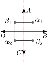
Figure 1: Toric and web diagram for the conifold. We have indicated the action of the orientifold involution studied in the text by the vertical red dashed line. The external legs in the web diagram are labeled for later convenience.

The correspondence between the toric and algebraic descriptions is explicit under the following map:

$$(\vec{\alpha},\vec{\beta})\mapsto(\xi,u,\sigma,w)=(\tfrac{1}{2}\,(\alpha_{1}\beta_{2}-\alpha_{2}\beta_{1}),\,\tfrac{1}{2}\,(\alpha_{1}\beta_{2}+\alpha_{2}\beta_{1}),\,-\alpha_{1}\beta_{1},\,\alpha_{2}\beta_{2})\,.$$ (20)

In these variables the orientifold involution acts as follows:

$$\alpha_{i}\leftrightarrow\beta_{i}\,.$$ (21)

We summarize the toric data for the resulting geometry in figure 1. Note, that this involution is not an automorphism of the resolved conifold. Instead, it is a map from a resolved conifold with Kähler modulus $t$ to a flopped conifold with modulus $-t$. Only for $t=0$ can we regard this as an involution that maps the conifold into itself.

As a consequence, the orientifold involution projects out the resolution mode of the conifold. On the other hand, the integral of the $B$-field over the exceptional $\mathbb{P}^{1}$ survives, since $B$ has an intrinsic minus sign under the action of $(-1)^{F_{L}}\Omega$.

Coming back to the $SU(5)$ and flavor stack, notice that the $\sigma=0$ divisor intersects the conifold at $\xi=\pm u$, which factorizes into a stack and its image, in accordance with the fact that the gauge symmetry is $SU(5)$. The $\{\xi=u\}\cap\{\sigma=0\}$ locus can be written in terms of GLSM coordinates as $\{\alpha_{2}\beta_{1}=\alpha_{1}\beta_{1}=0\}$, so we associate it with the Weil toric divisor $\beta_{1}=0$. Similarly, its $SU(5)$ image $\{\xi=-u\}\cap\{\sigma=0\}$ can be written as $\{\alpha_{1}\beta_{2}=\alpha_{1}\beta_{1}=0\}$, which is described by the Weil divisor $\alpha_{1}=0$, in accordance with the orientifold action (21). A similar exercise for $w=0$ shows that close to the conifold locus the flavor brane splits into a brane-image brane pair, associated with the $\alpha_{2}=0$, $\beta_{2}=0$ pair of toric Weil divisors.

Note that the $SU(5)$ stack factorizes without any approximation necessary, while factorization for the flavor stack at $w=0$ only happens as we zoom into the conifold singularity, since in (17) we dropped higher order terms. This distinction is not particularly important for the analysis in the rest of the paper. The subleading terms will affect the precise form of the effective action, but not the existence of the instanton contribution to the superpotential that we find, since the instanton lives at the singular locus.

3 IIB instanton computation via noncommutative crepant resolution

Our goal in this paper will be to understand the behavior of D-brane instantons living at the singularity appearing at weak coupling. The main difficulty in doing this is that, as we have just seen in the previous section, having F-theory $SU(5)$ models with a $\bf 10\,\bf 10\,\bf 5$ coupling of order one means that, in the weak coupling limit, one is forced to deal with a conifold singularity whose resolution mode is projected out by the orientifolding.

Indeed, this has been the main obstruction to studying these setups in perturbative string theory, since elementary algebro-geometric methods are not reliable on a singular space. Techniques for analyzing such systems, based largely on mirror symmetry, are known Hanany:2005ve ; Franco:2005rj ; Feng:2005gw ; Franco:2006es ; Franco:2007ii ; Forcella:2008au , and the result of applying such techniques will be briefly reviewed in §4 below. Nevertheless the application of these techniques involves a certain amount of heuristics (at least at the level that they are currently developed), so in the interest of making our derivation as assumption-free as possible, we have opted to give a first principles derivation of the physics at the singularity using the powerful technology of non-commutative crepant resolutions Bergh:aa ; Berenstein:aa (NCCRs in what follows). In practice, the NCCR approach gives us a concrete way of defining D-branes on the singular space, without referring to a small resolution. We will see that computing open string spectra is surprisingly easy in this language.

Armed with the knowledge of the instanton zero-modes present in our system, and how these couple to the background D7/D7-strings, we will be able, in §3.5, to reproduce very straightforwardly the $\bf 10\,\bf 10\,\bf 5$ interaction. We encourage the impatient reader to skip ahead to the derivation of the $\bf 10\,\bf 10\,\bf 5$ coupling in §3.5, and then return here for the systematic justification of the basic ingredients going into the computation.

3.1 NCCRs

Intuitively, the NCCR construction can be understood as a replacement of the coordinate ring $R=\mathbb{C}[u,\xi,\sigma,w]/(-\xi^{2}+u^{2}+\sigma w)$, describing the singular space, with the ring $A$ of open string modes of probe branes. This new ring $A$, which is also an algebra over $R$, can be thought of as the path algebra of the quiver. It is non-commutative, since paths cannot be composed in arbitrary order. The fact that the ring $R$ is singular implies that one cannot describe fractional branes easily, as these correspond to modules with infinitely long resolutions. On the other hand, the noncommutative ring $A$ is such that any module will admit a finite resolution. This is the essence of the noncommutative resolution. One further demands that $A$ be Cohen-Macaulay. This is the ring-theoretic analog of requiring a trivial canonical bundle, leading to an noncommutative crepant resolution (NCCR).

We define the conifold threefold algebraically by the equation

$$-\xi^{2}+u^{2}+\sigma\,w\,.$$ (22)

This variety has a coordinate ring $R=\mathbb{C}[\xi,u,\sigma,w]/(u^{2}-\xi^{2}+\sigma w)$, and admits a so-called matrix factorization, a pair of square matrices $(\phi,\psi)$ such that $\phi\cdot\psi=\psi\cdot\phi=(u^{2}-\xi^{2}+\sigma w)\cdot\mathbbm{1}$. From these two matrices, we can define two so-called maximal Cohen-Macaulay (MCM) modules over R. Essentially these are $R$-modules defined as the cokernels of the matrices

$$\phi=\begin{pmatrix}u-\xi&\sigma\\ -w&u+\xi\end{pmatrix}\,,\quad{\rm and}\quad\psi=\begin{pmatrix}u+\xi&-\sigma\\ w&u-\xi\end{pmatrix}\,.$$ (23)

We define

$$M \equiv {\rm coker}\big{(}\,R^{\oplus 2}\stackrel{{\scriptstyle\psi}}{{\longrightarrow}}R^{\oplus 2}\,\big{)}\,,$$ (24)

$$\tilde{M} \equiv {\rm coker}\big{(}\,R^{\oplus 2}\stackrel{{\scriptstyle\phi}}{{\longrightarrow}}R^{\oplus 2}\,\big{)}\,.$$ (25)

For the conifold, these are all the non-trivial irreducible MCM modules up to isomorphism. They are akin to line-bundles over the conifold, except that they fail to be locally free at the singularity. This can be understood by noticing that the matrices $\psi,\phi$ have rank one on the conifold, leaving a one-dimensional cokernel over every non-singular point. At the singularity, the matrices vanish, and the cokernels jump to dimension two. So we can think of these as Calabi-Yau filling branes with an added point-like brane at the origin.

These modules $M$ and $\tilde{M}$ over $R$ can be fit into exact complexes as follows:

(26)

We can think of $M$ and $\tilde{M}$ as the cokernels of the maps $\psi$ and $\phi$, respectively. Henceforth, we will replace $M$ or $\tilde{M}$ by their resolution complex as follows:

(27)

For our complexes, we use cohomological degree staring at zero on the right, and increasing as we move left. We will underline the zeroth position for clarity. The isomorphisms here state that our modules are simply the $H^{0}$ modules for these complexes.

Note, that these resolutions are semi-infinite, a hallmark of singular spaces. The goal of an NCCR is to replace $R$ with a ring such that all modules admit finite resolutions.

The NCCR for the singular ring $R$ is defined by picking one of these two modules, say $M$, and defining the endomorphism algebra $A={\rm End}(R\oplus M)$. $A$ turns out to be a noncommutative ring that will serve as our NCCR. It can be decomposed into four pieces

$$A=\underbrace{{\rm Hom}(R,R)}_{\cong R}\quad\oplus\quad\underbrace{{\rm Hom}(M,M)}_{\cong R}\quad\oplus\quad\underbrace{{\rm Hom}(R,M)}_{\cong M}\quad\oplus\quad\underbrace{{\rm Hom}(M,R)}_{\cong\tilde{M}}\,,$$ (28)

and can be encoded as the path algebra of the following quiver with relations:

Here, the arrows are morphisms that can be represented as cochain maps between resolution complexes. Take two complexes $K_{\bullet},C_{\bullet}$. Concretely, an element in Hom$(K_{\bullet},C_{\bullet})$ corresponds to a collection of vertical maps $f_{\bullet}$

(29)

such that each square commutes, i.e. $f_{i}\circ k_{i+1}=c_{i+1}\circ f_{i+1}$, and modulo homotopies, i.e. $f_{i+1}\sim f_{i+1}+g_{i}\circ k_{i+1}-c_{i+2}\circ g_{i+1}$ for some collection of the diagonal dotted $g_{i}$. These notions are reviewed in many physics papers, see Aspinwall:2004jr for a general account, and Collinucci:2014taa ; Collinucci:2014qfa for concrete examples.

Back to the conifold, the $\alpha_{1,2}:R\longrightarrow M$ can be written as follows

(30)

and for $\beta_{1,2}:M\longrightarrow R$

(31)

Finally, $e_{0}\in{\rm Hom}(R,R)\cong R$ and $e_{1}\in{\rm Hom}(M,M)\cong R$ are the multiplicative identities (actually idempotents) of the endomorphism ring of each node. These morphisms satisfy the relations:

$$\alpha_{1}\beta_{i}\alpha_{2}=\alpha_{2}\beta_{i}\alpha_{1}\,,\quad{\rm and}\quad\beta_{1}\alpha_{i}\beta_{2}=\beta_{2}\alpha_{i}\beta_{1}\,\quad{\rm for}\quad i=1,2\,,$$ (32)

where composition is defined from right to left. For instance, we see that

$$\alpha_{1}\beta_{1}\alpha_{2} = \begin{pmatrix}1\\ 0\end{pmatrix}\cdot(1,\,0)\cdot\phi\begin{pmatrix}0\\ 1\end{pmatrix}=\sigma\begin{pmatrix}1\\ 0\end{pmatrix}$$ (33)

$$\alpha_{2}\beta_{1}\alpha_{1} = \begin{pmatrix}0\\ 1\end{pmatrix}\cdot(1,\,0)\cdot\psi\begin{pmatrix}1\\ 0\end{pmatrix}=(u-\xi)\begin{pmatrix}0\\ 1\end{pmatrix}$$ (34)

The two column vectors differ by an element of the image of $\psi$:

$$\alpha_{2}\beta_{1}\alpha_{1}-\alpha_{1}\beta_{1}\alpha_{2}=\begin{pmatrix}-\sigma\\ u-\xi\end{pmatrix}=\psi\begin{pmatrix}0\\ 1\end{pmatrix}\,.$$ (35)

Such a morphism is discarded in the homotopy category as being gauge-equivalent to zero, and it actually corresponds to the zero morphism at the level of the cohomology.

The relations can be encoded in the superpotential $W=\alpha_{1}\beta_{1}\alpha_{2}\beta_{2}-\alpha_{1}\beta_{2}\alpha_{2}\beta_{1}$ which we recognize as the superpotential of the Klebanov-Witten theory Klebanov:1998hh .

The noncommutative crepant resolution is then simply defined as the ring $A$, which can be identified with the path algebra of the quiver modulo the relations derived from the superpotential. The product of the ring is the concatenation of arrows, and the sum is simply taking complex linear combinations of arrows.

D-branes are described in this formulation as complexes of right $A$-modules. More precisely, the bounded derived category D${}^{b}({{\rm mod-}A})$ comprises complexes of $A$-modules modulo certain equivalences known as quasi-isomorphism. The interest in the NCCR stems from the fact that this category D${}^{b}({{\rm mod-}A})$, which is defined entirely in the singular geometry, is known to be derived equivalent to the bounded derived category of coherent sheaves of the resolved conifold in both resolution phases. By studying D-branes through the NCCR, we sit in the middle between the two flopped phases, and are never forced to break our orientifold involution.

3.2 Quiver representations

$A$-modules are equivalent to representations of the quiver. We will be interested in two kinds of modules:

1. Modules that correspond to D7-branes. These can be regarded as infinite-dimensional representations.

2. Modules corresponding to fractional D$(-1)$-branes, which means D1 and anti-D1-branes wrapping the vanishing $\mathbb{P}^{1}$ of the conifold. These correspond to finite-dimensional representations.

We now explain how to construct these modules.

3.2.1 Recovering the conifold

As a warmup, we will study the finite-dimensional representation corresponding to a complete (non-fractional) D$(-1)$-brane. Physically, we expect the moduli space of this brane to be its transverse space, i.e. the conifold. By switching on FI terms in the quiver gauge theory, we can reach both flopped phases.

A (finite-dimensional) quiver representation consists in assigning a vector space to each node of the quiver, and promoting the arrows to linear maps between the vector spaces it connects. The idempotents $e_{0}$ and $e_{1}$ are set to one and left out of the diagram. In our case, we are interested in the following representation:

Denoting a representation by its dimension vector $\vec{d}$, in this case we have $\vec{d}=(1,1)$. We can interpret this as a single D$(-1)$-brane splitting up into one fractional brane on each node, leading to an abelian quiver theory. Here, the $\alpha_{i}$ and $\beta_{i}$ are simply complex numbers that transform in the (anti-)bifundamental of the relative $U(1)\subset U(1)\times U(1)$. In order to study the moduli space of $\vec{d}=(1,1)$ representations, we quotient out by the action of the relative $U(1)$. This leads us to a toric variety

$$\begin{array}[]{|c|c|c|c|}\hline\cr\alpha_{1}&\alpha_{2}&\beta_{1}&\beta_{2}\\ \hline\cr 1&1&-1&-1\\ \hline\cr\end{array}$$ (36)

We must also impose a D-term constraint

$$|\alpha_{1}|^{2}+|\alpha_{2}|^{2}-|\beta_{1}|^{2}-|\beta_{2}|^{2}=t\,.$$ (37)

The resolved phases correspond to $t>0$ and $t<0$. In our case, the orientifold involution (21) acts as $t\mapsto-t$, so it is not possible to respect it for non-zero $t$.

3.2.2 Non-compact branes

There are two basic infinite-dimensional representations $P_{0}$ and $P_{1}$, which are the projective right $A$-modules, defined as follows:

$$P_{0} = e_{0}\cdot A=\{\text{linear combinations of all paths ending on the lhs node `0'}\}$$ (38)

$$P_{1} = e_{1}\cdot A=\{\text{linear combinations of all paths ending on the rhs node `1'}\}$$ (39)

These can be thought of as CY-filling branes with line bundles on them. From these two modules, we can build all branes of interest through complexes. Let us now define how the orientifold involution $\sigma$ acts on a complex. Take a complex $K_{\bullet}$ of the form

(40)

where the cohomological degree increases from left to right. Then, the orientifold image of this complex is another complex $\tilde{K}_{\bullet}$ defined through the mapping $\Sigma$ which maps to objects of a complex as follows:

$$\Sigma:\quad K_{i}\longrightarrow\tilde{K}_{i}\equiv\sigma^{*}(K_{1-i})\,,$$ (41)

where depending on the choice of orientifold involution $\sigma^{*}(K_{1-i})$ may further act on the object $K_{1-i}$ (we will determine the proper action below), and it acts on the maps as follows:

$$\Sigma:\quad m_{i}\longrightarrow\tilde{K}_{i}\equiv\sigma^{*}(m_{i})^{T}\,.$$ (42)

Concretely, on a complex $K_{\bullet}$, we have the following action:

(43)

Let us now define the non-compact D7-branes of interest, which are supported over divisors. We will introduce a stack of brane/image-brane pairs called $G_{0}$ and $G_{1}$, where our $SU(5)$ theory will live:

$$G_{0}:\quad P_{1}\stackrel{{\scriptstyle\beta_{1}}}{{\longrightarrow}}\underline{P_{0}}\,,\qquad G_{1}:\quad P_{0}\stackrel{{\scriptstyle\alpha_{1}}}{{\longrightarrow}}\underline{P_{1}}\,.$$ (44)

We will also need a ‘flavor’ brane/image-brane pair:

$$F_{0}:\quad P_{1}\stackrel{{\scriptstyle\beta_{2}}}{{\longrightarrow}}\underline{P_{0}}\,,\qquad F_{1}:\quad P_{0}\stackrel{{\scriptstyle\alpha_{2}}}{{\longrightarrow}}\underline{P_{1}}\,.$$ (45)

We can easily see that $\Sigma:G_{0}\mapsto G_{1}$, and $\Sigma:F_{0}\mapsto F_{1}$ by applying the rules in (41) and (42), if we assume that $\sigma^{*}(P_{0,1})=P_{0,1}$, which is the choice compatible with the geometric action of our orientifold (as will become clear momentarily, when we map these complexes to sheaves).

How can we interpret these modules? One way is to study what happens when we promote the maps in the complexes to coordinates in the moduli space of the $\vec{d}=(1,1)$ representation. As we saw in the previous section, the $\alpha_{i}$ and $\beta_{i}$ become toric homogeneous coordinates for the conifold. Hence, we clearly see by inspection that, for instance, $G_{0}$ will correspond to a D-brane supported on the divisor $\beta_{1}=0$. The other piece of information we need is how to transport the projective modules to $P_{0}$ and $P_{1}$ to sheaves on the moduli space. In this case, one choice is to send

$$P_{0}\mapsto\mathcal{O}\,,\qquad P_{1}\mapsto\mathcal{O}(1)\,.$$ (46)

Hence, we conclude that our modules are mapped to sheaves as follows:

$$G_{0}: \quad\mathcal{O}(1)\stackrel{{\scriptstyle\beta_{1}}}{{\longrightarrow}}\underline{\mathcal{O}}\,,\qquad G_{1}:\quad\mathcal{O}\stackrel{{\scriptstyle\alpha_{1}}}{{\longrightarrow}}\underline{\mathcal{O}(1)}$$ (47)

$$F_{0}: \quad\mathcal{O}(1)\stackrel{{\scriptstyle\beta_{2}}}{{\longrightarrow}}\underline{\mathcal{O}}\,,\qquad F_{1}:\quad\mathcal{O}\stackrel{{\scriptstyle\alpha_{2}}}{{\longrightarrow}}\underline{\mathcal{O}(1)}$$

3.2.3 Fractional branes from the $(1,0)$ and $(0,1)$

The fractional branes, which in our case will be fractional D$(-1)$-instantons, correspond to the two simple (i.e. not admitting subrepresentations), one-dimensional representations: $S_{0}$ with $\vec{d}=(1,0)$, and $S_{1}$ with $\vec{d}=(0,1)$. As $A$-modules, these are simply defined as the modules generated by $e_{0}$ and $e_{1}$, respectively:

$$S_{0} = \mathbb{C}\langle e_{0}\rangle=\{\text{linear combinations of unique loop of length zero at node `0'}\}$$ (48)

$$S_{1} = \mathbb{C}\langle e_{1}\rangle=\{\text{linear combinations of unique loop of length zero at node `1'}\}$$ (49)

As quiver representations, each consists of a node with a $\mathbb{C}$, and the self-arrow $e_{0}=1$. Hence, these have no moduli. This is a reflection of the fact that these are fractional branes wrapping a rigid vanishing curve. These fractional branes admit the following projective resolutions:

(50)

In appendix A we show that these transport to D1 and anti-D1 branes wrapping the vanishing $\mathbb{P}^{1}$.

We can compute the Ext¹’s between these complexes by brute force. However, there is a much quicker way to do this, which exploits the fact that these are finite-dimensional representations. Suppose we want to compute Ext${}^{1}(S_{1},S_{0})$. This is equivalent to the so-called Yoneda-Ext group that parametrizes all possible non-trivial extensions of $S_{0}$ by $S_{1}$, i.e., exact sequences of the form

$$S_{1}\stackrel{{\scriptstyle a}}{{\longrightarrow}}E\stackrel{{\scriptstyle b}}{{\longrightarrow}}S_{0}$$ (51)

such that $E\not\cong S_{0}\oplus S_{1}$. Clearly, the middle object $E$, which will depend on the choice of maps $(a,b)$, must always have dimensions $\vec{d}=(1,1)$. Hence, we can draw an exact sequence of quiver representations as follows:

(52)

In this sequence, we have omitted the zeroes corresponding to empty quiver nodes. However, these are important, because arrows going to and from empty nodes are the zero map. A sequence of quiver representations means all squares must commute. In the upper $(0,1)$ quiver representation, the arrows going to the left are zero. Hence, we must impose that the composition $\beta_{i}\circ a=0$ for $i=1,2$, which implies $\beta_{i}=0$.

For each choice of the pair $\alpha_{i}$ we have an exact sequence of quiver representations. Hence, Ext${}^{1}(S_{1},S_{0})\cong\mathbb{C}^{2}\cong(\alpha_{1},\alpha_{2})$. For the zero element of this group, i.e. $\vec{\alpha}=0$, we see indeed that the middle element is isomorphic to $S_{0}\oplus S_{1}$. We can take this one step further by modding out these maps by the $\mathbb{C}^{*}$ that acts homogeneously on these two maps, and excluding the trivial map. This yields a $\mathbb{P}^{1}$. We can think of this as the exceptional curve after resolving, since it corresponds to the moduli space for the recombination tachyon between an D1 and and anti-D1 with a net flux difference of $\mathcal{O}(1)$. In other words, we could think of this $\mathbb{P}^{1}$ as the moduli space of the induced D$(-1)$-brane trapped on this pair. Alternatively, in field theory terms we have that the fact that we have $\beta_{i}=0$ implies that all mesons vanish, so we are stuck at the exceptional locus of the resolution.

Similarly, we deduce that Ext${}^{1}(S_{0},S_{1})\cong\mathbb{C}^{2}$. Finally, we will define our fractional branes as follows:

$$I_{0}\equiv S_{0}[-1]\,,\qquad I_{1}\equiv S_{1}[-1]\,.$$ (53)

Where we have shifted our complexes one position to the right (in the conventions of Aspinwall:2004jr ) to take into account that the D1 brane mutually supersymmetric with respect to a D7 brane wrapping an arbitrary cycle is, from the perspective of sheaves, the anti-brane of the skyscraper sheaf Bershadsky:1995qy . The spectrum between these two will not change under a simultaneous shift. However, the spectrum with the non-compact branes will.

3.3 Ext’s

Let us now compute the Ext groups involving the flavor branes. We have already established in the previous section that:

$${\rm Ext}^{1}(I_{0},I_{1})\equiv{\rm Ext}^{1}(I_{1},I_{0})\equiv\mathbb{C}^{2}\,.$$ (54)

Let us now calculate the spectra involving the non-compact branes. We will do a few sample calculations and then list the results for all sectors. Let us start with the spectrum between $G_{0}$ and $I_{0}$. It is given by the Ext${}^{i}(G_{0},I_{0})$ groups which correspond to cochain maps, whereby the degree $i$ instructs us to shift the second complex to the right as follows:

$${\rm Ext}^{i}(G_{0},I_{0})\equiv{\rm Hom}_{D^{b}({\rm mod-}A)}(G_{0},I_{0}[i])\,.$$ (55)

The fact that this is computed in the derived category of modules means that we have to quotient out by quasi-isomorphisms. Fortunately, it is known fact that if a ring has enough projectives, as it is the case here, it is sufficient to consider projective resolutions and quotient out by cochain homotopies (explained around formula (29)).

Let us then compute Ext${}^{1}(G_{0},I_{0})$. Since $I_{0}=S_{0}[-1]$, we see that Ext${}^{1}(G_{0},I_{0})\cong$ Ext${}^{0}(G_{0},S_{0})$. So the task is to find the vertical maps $(f_{0},f_{1})$ in the following diagram:

(56)

Let us start with $f_{0}$. For consistency, it is necessarily of the form

$$f_{0}=z+(\ldots)\circ\beta_{1}+(\ldots)\circ\beta_{2}$$ (57)

with $z$ a complex number. The elided parts can be arbitrarily complex, but since they are composed with $\beta_{i}$ on the right they always give contributions to $f_{0}$ which are homotopy equivalent to zero, so we can simply forget about these and set $f_{0}=z$. Then, in order for the square to commute, the only solution is $f_{1}=(z,0)^{T}$, which is also non-trivial w.r.t. homotopy. In conclusion, Ext${}^{1}(G_{0},I_{0})\cong\mathbb{C}$, where $\mathbb{C}$ is parametrized by the number $z$. The rest of the D1/D7 Ext groups are computed in the same manner.

We list the Ext groups between fractional and non-compact branes here:

$${\rm Ext}^{i}(G_{0},I_{0}) = (0,\mathbb{C},0,0)\,,\qquad{\rm Ext}^{i}(G_{0},I_{1})=(0,0,\mathbb{C},0)\,,$$ (58)

$${\rm Ext}^{i}(G_{1},I_{0}) = (0,0,\mathbb{C},0)\,,\qquad{\rm Ext}^{i}(G_{1},I_{1})=(0,\mathbb{C},0,0)\,,$$ (59)

$${\rm Ext}^{i}(F_{0},I_{0}) = (0,\mathbb{C},0,0)\,,\qquad{\rm Ext}^{i}(F_{0},I_{1})=(0,0,\mathbb{C},0)\,,$$ (60)

$${\rm Ext}^{i}(F_{1},I_{0}) = (0,0,\mathbb{C},0)\,,\qquad{\rm Ext}^{i}(F_{1},I_{1})=(0,\mathbb{C},0,0)\,.$$ (61)

Since the spectrum between two non-compact branes is infinite-dimensional, the calculation is qualitatively different. Let us perform a sample calculation, say Ext${}^{1}(G_{0},G_{1})$. It consists in the set of vertical maps $f_{1}\sim f_{1}+g_{0}\circ\beta_{1}-\alpha_{1}\circ g_{1}$ modulo homotopies given by $(g_{0},g_{1})$

(62)

Here, we see that any loop from node ‘1’ to itself not made of $\beta_{1}$ at its start or $\alpha_{1}$ at its end is allowed. In other words, we can take any linear combination of any power of $\beta_{2}\circ\alpha_{2}$. Hence, we conclude that our Ext group is a polynomial ring Ext${}^{1}(G_{0},G_{1})\cong\mathbb{C}[\beta_{2}\alpha_{2}]$. This is nothing other than the ring of polynomials on the complex plane. This reflects the fact that our D7-branes intersect over a complex plane, and the low energy bifundamental strings are simply fields defined on it. In this non-compact setup, this spectrum is an infinite-dimensional vector space. However, upon compactifying the intersection curve of the two D7-branes, the spectrum will become finite-dimensional, and upon switching on an appropriate flux, it will be chiral. Note that this information is input from the point of view of the theory at the conifold singularity. Below we will choose this input to be that appearing in F-theory GUT models.

The other D7/D7 spectra are computed in the same manner, with the results:

$${\rm Ext}^{i}(G_{0},G_{1}) = (0,\mathbb{C}[\alpha_{2}\beta_{2}],0,0)\,,\qquad{\rm Ext}^{i}(G_{0},F_{1})=(0,\mathbb{C}[\alpha_{1}\beta_{2}],0,0)\,,$$ (63)

$${\rm Ext}^{i}(G_{1},G_{0}) = (0,\mathbb{C}[\beta_{2}\alpha_{2}],0,0)\,,\qquad{\rm Ext}^{i}(G_{1},F_{0})=(0,\mathbb{C}[\beta_{1}\alpha_{2}],0,0)\,,$$ (64)

$${\rm Ext}^{i}(F_{0},F_{1}) = (0,\mathbb{C}[\alpha_{1}\beta_{1}],0,0)\,,\qquad{\rm Ext}^{i}(F_{0},G_{1})=(0,\mathbb{C}[\alpha_{2}\beta_{1}],0,0)\,,$$ (65)

$${\rm Ext}^{i}(F_{1},F_{0}) = (0,\mathbb{C}[\beta_{1}\alpha_{1}],0,0)\,,\qquad{\rm Ext}^{i}(F_{1},G_{0})=(0,\mathbb{C}[\beta_{2}\alpha_{1}],0,0)\,.$$ (66)

The resulting quiver is shown in figure 2.

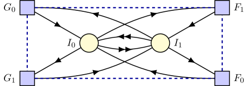
Figure 2: Quiver representation for the theory discussed in the text, before taking the orientifold involution (described by a reflection with respect to a horizontal line through the quiver nodes, as described in §3.4). We have indicated the matter between the flavor branes by the blue dashed line, the actual matter content coupling to the quiver degrees of freedom will depend on choices of flux away from the singularity.

3.4 Orientifold projection

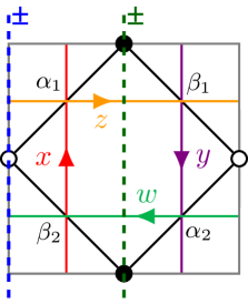
(a) Action on the dimer model.

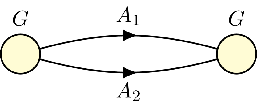
(b) Resulting quiver.

Figure 3: Action of the orientifold studied in the text on the quiver theory of the conifold. 3(a) The action on the dimer model Hanany:2005ve ; Franco:2005rj ; Feng:2005gw is given by a line orientifold, in the terminology of Franco:2007ii . The choice of equal signs for the two fixed lines is associated with having an O7 plane instead of an O3 plane. 3(b) Resulting quiver gauge theory. We will determine in the text that $G=U\!Sp(2N)$.

We would now like to understand the nature of the orientifold projection acting on the singular conifold. I.e. which projection should we take on the quiver found in figure 2. Recall from §2 that, for a conifold defined as

$$\xi^{2}=u^{2}+\sigma w$$ (67)

the orientifold involution acted geometrically as $\xi\to-\xi$, leaving the other coordinates invariant. If we rewrite this conifold as $xy=zw$, with $(x,y,z,w)=(u+\xi,u-\xi,-\sigma,w)$, the orientifold action is

$$x\leftrightarrow y\quad;\quad z\leftrightarrow z\quad;\quad w\leftrightarrow w\,.$$ (68)

For the $(1,1)$ representation of the quiver, these geometric coordinates are in one-to-one correspondence with vevs of the elementary mesons of the quiver theory. The conifold theory admits various involutions, but it is easy to see (from the classification in Franco:2007ii , for instance) that the only class of involutions compatible with the action (68) on the mesons is the action shown in figure 3(a). In principle the projection associated to the two fixed lines can be independently chosen, but as discussed in detail in Garcia-Etxebarria:2015lif the choice with opposite relative signs corresponds to an O3 plane, instead of an O7 plane, so we need to choose the two fixed lines to have the same sign. The resulting theory is depicted in figure 3. We still have the ambiguity of whether the gauge group on the nodes is of type $SO(N)$ or $U\!Sp(2N)$.

One can easily see that the right choice is $G=U\!Sp(2N)$ by a probe argument, as follows. In our setup we have an O7^- plane coming out of the conifold point. We know that in flat space a single D3 brane on top of an O7^- gives rise to a four dimensional $\mathcal{N}=2$ $U\!Sp(2)$ theory (it would be a $SO(2)$ algebra for a O7⁺). This will also be true at low energies for a D3 on the orientifolded conifold background, as long as the D3 is on top of the O7^- plane but away from the singular point. This implies that there should be a submanifold on the moduli space of the $G\times G$ theory for $N=1$ where at low energies one recovers the $\mathcal{N}=2$ $U\!Sp(2)$ theory. A single probe brane on the orientifolded conifold background will have gauge group $SO(2)\times SO(2)$ or $U\!Sp(2)\times U\!Sp(2)$, since it corresponds to two D3 branes on the covering space. Out of these two choices, the only one that can Higgs to a $U\!Sp(2)$ subgroup anywhere in the moduli space is $U\!Sp(2)\times U\!Sp(2)$, so we conclude that the right projection is $U\!Sp(2N)\times U\!Sp(2N)$.

The fact that we obtain a $U\!Sp(2N)\times U\!Sp(2N)$ projection on the quiver will be essential in order to be able to understand the $E_{6}$ Yukawa coupling in the superpotential as coming from an instanton: in the F-theory background we have no gauge dynamics localized at the Yukawa point, so we need to set $N=0$, and $U\!Sp(0)$ nodes in empty quivers are precisely those which can give rise to stringy instanton effects Aganagic:2003xq ; Intriligator:2003xs ; Aganagic:2007py ; GarciaEtxebarria:2008iw . The microscopic reason for this is that the projection on spacetime filling branes and the corresponding instantonic branes is reversed Argurio:2007qk ; Argurio:2007vqa ; Bianchi:2007wy ; Ibanez:2007rs (see also Blumenhagen:2009qh for a review), so a $U\!Sp$ projection on fractional D3 branes implies the existence of an orthogonal projection on the fractional D$(-1)$ branes. This is precisely the projection necessary for eliminating the neutral $\overline{\tau}$ modes on D-brane instantons, and allowing for the existence of a superpotential contribution.

The previous argument is somewhat indirect, and it may be illuminating to see explicitly the enhancement in moduli space. In the rest of this section we do this exercise. (The reader not interested in this derivation should feel free to skip ahead to the next section.)

In addition to the quiver in figure 3(b), there is a superpotential of the form Imai:2001cq

$$W=\varepsilon_{ij}\varepsilon_{lm}\operatorname{Tr}(\gamma_{G}A_{i}\gamma_{G}A_{l}^{t}\gamma_{G}A_{j}\gamma_{G}A_{m}^{t})\,.$$ (69)

If $G$ is $U\!Sp(2N)$ then $\gamma_{g}=\operatorname{diag}(\sigma_{2},\ldots,\sigma_{2})$ with $\sigma_{2}$ the Pauli matrix $\left(\begin{smallmatrix}0&-i\\ i&0\end{smallmatrix}\right)$, and for $G=SO(M)$ we have $\gamma_{G}=\mathbbm{1}$. Notice that for $G=U\!Sp(2)$ the superpotential (69) identically vanishes, so we only need to worry about D-terms. Decompose $A_{1}=a^{(1)}_{\mu}\sigma_{\mu}$, with $\sigma_{\mu}=(\mathbbm{1},i\sigma_{i})$ and $\sigma_{i}$ the Pauli matrices. Elements of $U\!Sp(2)\times U\!Sp(2)$ act on $a^{(1)}_{\mu}$ as $SO(4)$ rotations. Note that these rotations act independently on the real an imaginary parts of $a_{\mu}$. Let us go to a gauge in which $\Re(a^{(1)}_{\mu})=(a_{0},0,0,a_{3})$ with $(a_{0},a_{3})\neq(0,0)$. (This will be the generic case for either the real or imaginary part of one of the $A_{i}$ fields, we choose to talk about the real part of $A_{1}$ for concreteness. It may be the case that $a_{0}=0$ or $a_{3}=0$ for all $A_{i}$ at certain points in moduli space, we will analyze these points momentarily.)

Non-abelian D-terms for this theory are given by

$$\sum_{i}\operatorname{Tr}(A_{i}^{\dagger}A_{i}\sigma_{k})=\sum_{i}\operatorname{Tr}(A_{i}A_{i}^{\dagger}\sigma_{k})=0$$ (70)

for any of the three Pauli matrices $\sigma_{k}$. With the gauge choice above, these imply that we can write

$$A_{i}=z_{i}^{0}+iz_{i}^{3}\sigma_{3}\,.$$ (71)

We see that the $U\!Sp(2)\times U\!Sp(2)$ gauge symmetry is broken down to a $U(1)\times U(1)$

$$A_{i}\to e^{-i\alpha\sigma_{3}}A_{i}e^{i\beta\alpha_{3}}$$ (72)

together with the $\mathbb{Z}_{2}$ action

$$A_{i}\to(-i\sigma_{1})A_{i}(i\sigma_{1})\,.$$ (73)

There is an overall $U(1)$, obtained when $\alpha=\beta$, which acts trivially on $A_{i}$. The nontrivial $O(2)=U(1)\rtimes\mathbb{Z}_{2}$ symmetry can be understood in the representation of the $A_{i}$ as four-vectors as the rotations and reflection on the 2-plane of non-vanishing directions, associated to $\sigma_{0}$ and $\sigma_{3}$. Introduce the coordinates $u_{i}^{\pm}=z_{i}^{0}\pm iz_{i}^{3}$. It is easy to see that (72) acts on these coordinates as $u_{i}^{\pm}\to e^{\pm i(\beta-\alpha)}u_{i}^{\pm}$. Furthermore, the non-abelian D-terms (70) become in these coordinates the single equation

$$\sum_{i}|u_{i}^{+}|^{2}=\sum_{i}|u_{i}^{-}|^{2}\,.$$ (74)

We recognize this moduli space as the usual GLSM construction of the conifold given above with $u_{i}^{+}=\alpha_{i}$ and $u_{i}^{-}=\beta_{i}$, together with a decoupled $U(1)$ factor, associated with the $U(1)$ symmetry of a D3 in flat space.

The geometric involution we are interested in appears here as the remnant discrete $\mathbb{Z}_{2}$ action (73), which acts on the $u_{i}^{\pm}$ coordinates as $u_{i}^{\pm}\leftrightarrow u_{i}^{\mp}$. The fixed point locus is obtained whenever $u_{i}^{\pm}=u_{i}^{\mp}$ (in some gauge). This implies $z_{i}^{3}=0$ (in this gauge, or equivalently $z_{i}^{0}=0$ in a different gauge), and assuming $z^{0}_{1}z_{2}^{0}\neq 0$ on this locus we have an enhanced $U\!Sp(2)$ symmetry, in agreement with the expected behavior of the D3 on the O7^- plane.

3.5 Instanton effects in the orientifolded background

Let us now focus on the specific choice of ranks that will arise in GUT models, as described in §2. We take in particular multiplicity 5 for the $G_{i}$ stacks (so they will be associated with the GUT stack) and multiplicity 1 for the $F_{i}$ stacks (associated with the flavor brane). For simplicity, we choose the spectrum between the $G_{i}$ branes to be given by a single chiral bifundamental, which upon orientifolding will give rise to the 10 representation. For phenomenological purposes it is often more interesting to take three copies of the 10 representation, we generalize the analysis below. We also choose to have a single 5 between the $G_{i}$ and $F_{i}$ stacks, with the same chirality as the 10. With these choices, the theory after orientifolding is that described in figure 4.

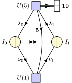
Figure 4: The theory obtained after orientifolding the theory in figure 2. The quiver nodes $I_{i}$ have symplectic gauge factors, formally given by $U\!Sp(0)$ in the absence of probe branes.

The instanton effects come from euclidean D1 branes wrapping the (empty) $I_{i}$ nodes. We will consider the case of a single fractional instanton wrapping either $I_{0}$ or $I_{1}$. (Contributions due to multi-instantons may be interesting, but their analysis is significantly more subtle so we leave the analysis of these to the interested reader.) Note that due to our choice of chirality for the 10 and 5 representations the two nodes behave rather differently. Let us start with $I_{1}$. In our conventions, the $I_{1}$ node admits terms in the instanton action coupling the zero modes $\lambda_{1},\nu_{1}$ to matter fields of the form

$$S_{\text{inst}}=c\,{\bf 10}_{[ij]}\,\lambda_{1}^{\bar{i}}\,\lambda_{1}^{\bar{j}}+d\,\lambda_{1}^{\bar{i}}\,{\bf 5}^{i}\,{\nu_{1}}$$ (75)

for some $c,d\in\mathbb{C}$. We have indicated the $U(5)$ indices explicitly. This instanton action, upon integration of the fermionic zero modes $\lambda_{1},\nu_{1}$, will generate an effective $\bf 10\,\bf 10\,\bf 5$ coupling in the low-energy theory, in agreement with the F-theory expectation.

On the other hand, the euclidean D-brane on $I_{0}$ behaves very differently. Gauge invariance forbids any couplings analogous to (75), so due to the unsaturated zero modes the instanton will generate a higher F-term, instead of a superpotential contribution Beasley:2004ys ; Beasley:2005iu .

Let us now argue that the couplings in (75) do in fact appear in the instanton action. In both terms, the matter fields correspond to recombination modes of the flavor stacks. In the first case, $G_{0}$ and $G_{1}$ are Weyl divisors that cannot leave the singularity. Indeed, if the $\bf 10$ field is turned off, the charged zero-modes are always massless. Recombination of the $G_{0}$ and $G_{1}$ divisors in order to obtain a Cartier divisor not intersecting the singularity will manifest itself, from the point of view of the instanton, in giving masses to the $\lambda_{1}^{\bar{i}}$ modes. The mass term transforms in the $\bf 10$ representation of $SU(5)$, and can indeed be seen as the expectation value of the corresponding GUT matter field (which is, from the instanton worldvolume point of view, a background field). A similar argument holds for the second term in (75).

3.6 Yukawa rank in the multiple family case

For simplicity we have considered the case in which there is a single ${\bf 10}$ representation involved in the Yukawa coupling of interest. In realistic models one would like to have three generations, often all living on the same curve. The most general instanton action is now given by

$$S_{\text{inst}}=c_{I}\,{\bf 10}^{I}_{[ij]}\,\lambda_{1}^{\bar{i}}\,\lambda_{1}^{\bar{j}}+d\,\lambda_{1}^{\bar{i}}\,{\bf 5}^{i}\,{\nu_{1}}$$ (76)

with $I$ the family index. The resulting Yukawa matrix is proportional to

$$\begin{pmatrix}c_{1}^{2}&c_{1}c_{2}&c_{1}c_{3}\\ c_{1}c_{2}&c_{2}^{2}&c_{2}c_{3}\\ c_{1}c_{3}&c_{2}c_{3}&c_{3}^{2}\end{pmatrix}$$ (77)

which, as already remarked in Blumenhagen:2007zk , is of rank one. This is in agreement with the general expectation from the F-theory analysis Cecotti:2009zf .

4 Mirror description

The previous results can also be justified, to some extent, from the point of view of the IIA mirror description of the conifold using the techniques in Hori:2000ck ; Feng:2005gw . In particular, the structure of the mirror manifold in the presence of the orientifold involution of interest to us has been discussed in Franco:2007ii . One additional ingredient with respect to the discussion in Franco:2007ii is the presence of flavor branes. How to include these in the present context was discussed in Franco:2006es ; Forcella:2008au . Note that the discussion in these works involves a nontrivial amount of guesswork, which is why we have chosen to give a more principled analysis above. Nevertheless the mirror picture is technically simpler to analyze, so we will briefly describe it here in order to provide some additional intuition for the reader.

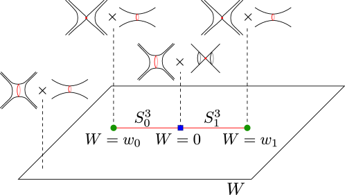
Figure 5: Mirror for the conifold, as a fibration over $\mathbb{C}$, parameterized by a coordinate $W$. The generic fiber is $\mathbb{C}^{*}$ times $\mathbb{P}^{1}$ punctured at four points. The $\mathbb{C}^{*}$ fiber degenerates at $W=0$, and the punctured $\mathbb{P}^{1}$ at $W\in\{w_{0},w_{1}\}$. The mirror of the fractional branes on the conifold wrap the three-spheres $S^{3}_{0}$ and $S^{3}_{1}$, obtained by fibering the product of the degenerating 1-cycles in the fiber over the segment in the base.

As described in Hori:2000ck ; Feng:2005gw , for the purposes of computing chiral information one can take the mirror of the conifold to be described by a $\mathbb{C}^{*}\times\Sigma$ fibration over $\mathbb{C}$ given by the equations

$$uv =W$$ (78)

$$P(x,y) =W$$ (79)

with $u,v,W\in\mathbb{C}$, $x,y\in\mathbb{C}^{*}$. The complex plane is parameterized by $W$. The first equation gives a $\mathbb{C}^{*}$ fiber over the $W$ plane, with a degeneration at $W=0$. The second equation defines a Riemann surface fiber with four punctures. We pick coordinates and a framing Bouchard:2011ya such that

$$P(x,y)=q+y+xy-xy^{2}\,.$$ (80)

Here $q$ encodes the complex structure of the mirror, or equivalently the complexified Kähler modulus of the original conifold. The resulting Riemann surface is singular for $W=q$ and $W=q+1$; we denote these points $w_{0},w_{1}$ respectively. Consider the $T^{2}$ over any point in the $W$ plane formed by the $S^{1}\subset\mathbb{C}^{*}$ collapsing at $W=0$ times the one-cycle in $\Sigma$ associated with the degenerations at $w_{i}$. The total space of this $T^{2}$ over a segment in the $W$ plane connecting $W=0$ and $w_{i}$ has the topology of $S^{3}$, and the two fractional branes of the conifold are obtained by wrapping D6 branes on these cycles. The resulting geometry is depicted in figure 5.

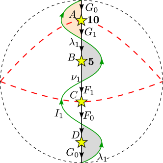
Figure 6: Schematic structure of the fiber of the mirror above the $W=0$ point. The fiber is topologically a disk with four punctures (denoted by stars), mapped here to a disk in which the dashed boundary should be identified to a point. The fixed locus of the orientifold involution is given by the red dashed line. The green line denotes the intersection of the $I_{1}$ euclidean D2 brane with the Riemann surface, and the black segments between puntures indicate the location of the flavor branes. We have also indicated by the shaded disks the worldsheet instantons giving rise to (75).

These two fractional branes intersect over $W=0$. We will focus on the structure of the $\Sigma$ fiber over this point, which is described by $\{q+y+xy-xy^{2}\}\subset(\mathbb{C}^{*})^{2}$. The structure of the fiber at this point is summarized in figure 6. As we see from this figure, in this mirror description various nontrivial aspects of the IIB analysis are manifest. The structure of zero modes and chiral multiplets arises in a simple way from brane intersections (perhaps at infinity along a puncture, as for the 5 and 10 matter fields), and the couplings in the instanton effective action (75) arise naturally from worldsheet instanton effects.

5 M-theory description

In this section we would like to reproduce some of the effects we have observed in the weakly coupled IIB and IIA descriptions directly in the more usual (in the F-theory model building literature) geometric M-theory language. We will focus on two interrelated effects. The first effect we would like to understand is simply how the usual computation of Yukawa couplings in M-theory language, that is, in terms of M2 branes wrapping appropriate chains with boundaries on the matter states Marsano:2011hv ; Martucci:2015dxa ; Martucci:2015oaa , connects to the instantonic picture.

At a heuristic level it is not hard to argue that there is a connection, as follows. The IIA configuration T-dual to the fractional D$(-1)$ on the conifold is given by D2 brane wrapping the T-duality cycle, and the exceptional $\mathbb{P}^{1}$ of the conifold. At the edges of the T-duality interval we have O6 planes, and the $\mathbb{P}^{1}$ of the conifold necessarily collapses there. On a generic point along the interval the $\mathbb{P}^{1}$ is not necessarily of zero size. The D2 instanton wraps the total space of this $\mathbb{P}^{1}$ fibration over the interval, which defines a non-trivial three-cycle $\Sigma_{3}$.

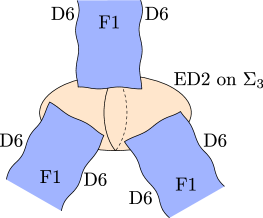
(a) Instanton mediated coupling.

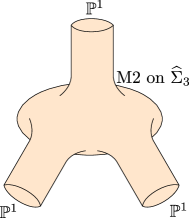
(b) M-theory uplift.

Figure 7: 7(a) Schematic viewpoint of a instanton mediated coupling. Massless open strings between background D6 branes meet at the location of an euclidean D2 brane, which (assuming the right zero mode structure) can mediate an effective coupling. 7(b) Its M-theory uplift, where the whole configuration has recombined into a non-compact three-cycle with three $\mathbb{P}^{1}$ boundaries.

Consider now in the IIA picture for a coupling mediated by D2-brane instantons. This is depicted in figure 7(a). We have that various open string states meeting at a given spacetime point, where the euclidean D2-brane lives, giving rise to the effective vertex in the low energy action. In the M-theory picture both the D2 and the F1 lift to M2 branes, so the lift of the IIA configuration will be given by a recombined smooth M2, shown in figure 7(b). This M2 wraps the three-chain $\widehat{\Sigma}_{3}$, with boundaries given by $\mathbb{P}^{1}$ cycles associated with the states appearing in the coupling. This is precisely the usual description for how perturbative couplings (such as the $\bf 10\,\bf 10\,\bf 5$ coupling of interest to us) appear in the M-theory description Marsano:2011hv ; Martucci:2015dxa ; Martucci:2015oaa .

We can understand the transition from figure 7(a) to 7(b) as follows. Focus on a junction where an open F1-worldsheet stretched between two D6-branes ends on an interval on the Euclidean D2-brane, say the upper junction in 7(a). Now take Euclidean $\tau$ time to run horizontally from left to right in the diagrams. Then, at each slice with constant $\tau$ we have a semi-infinite line from the F1 ending on the D2. From the point of view of the D2-worldvolume, the F1 is an electric source, and a backreacted solution creates a funnel-type geometry, whereby the F1 is replaced by a smooth spike made entirely of the D2-brane Callan:1997kz . At any horizontal slice, the boundary of this surface is a circle, whose radius grows with $g_{s}$. This system lifts straightforwardly to a smooth M2 brane configuration in M-theory. This recombination process is shown in figure 8.

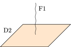
(a) Weakly coupled viewpoint.

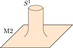
(b) M-theory uplift.

Figure 8: A fundamental string ending on a D2 brane lifts to a smooth funnel-like solution for the M2 brane in M-theory.

Now take a family of these funnel geometries parametrized by $\tau$, covering the whole interval. At the two extremities $g_{s}$ vanishes, since there are D6-branes there. Hence, the boundary circles of the M2 funnels shrink to zero size at the extremities of the interval. In the end, the full boundary of this family is a circle fibration over the interval collapsing over two points, i.e. an $S^{2}$. Now we have replaced the F1/D2-junction with a smooth D2 with boundaries, which trivially uplifts to M-theory to an M2 with boundaries, as depicted in 7(b).

In what follows we will present evidence supporting this heuristic picture, by explicitly tracking the M-theory three-chain $\widehat{\Sigma}_{3}$ to the weak coupling limit, and seeing that it survives the limit, getting localized at the $E_{6}$ point. A full proof of the connection requires an explicit identification of $\widehat{\Sigma}_{3}$ with the uplift of the D2 brane. It would be very interesting to work this out in detail, but we will not do this here.

Along the way we will find that in the strict weak coupling limit ($g_{s}=0$), the geometry develops a non-flat fiber at the $E_{6}$ point. This effect only appears at $g_{s}=0$, and disappears as long as $g_{s}$ is finite, no matter how small. We conjecture that the physical origin for this effect has to do with the light strings appearing for vanishing $B$-field on the collapsed cycle.

This conjecture is based on the following observations. Notice first that in the weakly coupled description this $B$-field period can be arbitrarily tuned while staying on the quiver locus (contrary to what is stated in Donagi:2009ra ), so it is possible to enhance the contribution of the instanton by tuning the $B$-field. More in detail, the instanton contribution to the superpotential goes as

$$\Delta_{np}W=(\ldots)e^{-\frac{1}{g_{s}}\int_{\mathbb{P}^{1}}B_{2}+\int_{\mathbb{P}^{1}}C_{2}}\,\bf 10\,\bf 10\,\bf 5$$ (81)

where we have omitted the (unknown) dependence on the complex structure moduli, and schematically indicated by $\int_{\mathbb{P}^{1}}B_{2}$ and $\int_{\mathbb{P}^{1}}C_{2}$ the periods of the $B_{2}$ and $C_{2}$ fields on the non-resolvable $\mathbb{P}^{1}$. (This is schematic since the $\mathbb{P}^{1}$ is never present in the geometry as a proper algebraic cycle, but the corresponding periods are still well defined.) We see that taking $\int_{\mathbb{P}^{1}}B_{2}\to 0$ we enhance the magnitude of the non-perturbative effect. Nevertheless, we cannot simply take $\int_{\mathbb{P}^{1}}B_{2}$ to vanish. This is because in order to have a standard field theory description of the conifold background one needs the $B$ field on the collapsing $\mathbb{P}^{1}$ not to vanish Strominger:1995cz ; Aspinwall:1995zi . Otherwise one has massless strings coming from D3 branes wrapping the collapsing $\mathbb{P}^{1}$. The mass of these states is, in fact, given by the same expression as the instanton action. Our conjecture is that these D3 branes dualize to M5 branes wrapping the non-flat fiber. Assuming that this identification is correct, the IIB analogue of the disappearance of the non-flat fiber as we take $g_{s}$ nonzero is presumably related to some dynamical effect on the D3 making it massive. Also, the D3 branes on the type IIB side get a mass by turning on a $B$-field background, which should imply that the M5 branes on the non-flat fiber get a mass upon turning on an appropriate $C_{3}$ background. It would be very interesting to verify (or refute) our conjectured identification, and to understand the mechanisms behind both mass mechanisms, but we will not attempt to do so here.

5.1 The weak coupling limit

We will start by reviewing the techniques in Donagi:2012ts ; Clingher:2012rg , which provide an efficient way of taking a weak coupling limit in F-theory such that one can more easily recognize the IIB brane system encoded by an elliptic fibration, elaborating on Sen’s original proposal Sen:1996vd ; Sen:1997gv . We will first describe the procedure in Donagi:2012ts ; Clingher:2012rg in general, and then apply it to the $SU(5)$ model.

Let us start with the following particular form for an elliptic fibration:

$$W:\quad-y^{2}+x^{3}+b_{2}x^{2}z^{2}+2\,b_{4}xz^{4}+b_{6}z^{6}$$ (82)

Following Sen Sen:1996vd ; Sen:1997gv , we introduce a small parameter $\epsilon$ and rescale $(b_{4},b_{6})\mapsto(\epsilon b_{4},\epsilon^{2}b_{6})$, then we find that the $j$-function of this model blows up everywhere except at $b_{2}=0$. In this way, the discriminant has the following leading term:

$$\Delta=\epsilon^{2}b_{2}^{2}(b_{4}^{2}-b_{2}b_{6})+\mathcal{O}(\epsilon^{3})\,.$$ (83)

As explained in Sen:1996vd ; Sen:1997gv , there is an O7-plane at $b_{2}=0$ and a D7-brane at $b_{4}^{2}-b_{2}b_{6}=0$. The problem with this approach to the weak coupling limit stems from the fact that taking $\epsilon\rightarrow 0$ does not commute with computing the discriminant of the elliptic fibration. In order to see Sen’s result, one must first keep $\epsilon$ arbitrary, compute the discriminant, and only then expand. If, on the other hand one first expands the Tate equation in $\epsilon$ and then takes the limit, then the model washes away all the D7-brane data, giving too crude a rendition of the situation.

One can improve on this by adopting the philosophy of Donagi:2012ts ; Clingher:2012rg , and promoting the parameter $\epsilon$ to a coordinate. So we study the fivefold $X_{5}$, which is a family of CY fourfolds, of which the limiting hypersurface $\epsilon=0$ would be the weakly coupled F-theory model. $X_{5}$ is then given by the hypersurface equation:

$$X_{5}:\quad y^{2}=x^{3}+b_{2}x^{2}z^{2}+2\,\epsilon b_{4}xz^{4}+\epsilon b_{6}z^{6}\,.$$ (84)

One first notices that this fivefold is singular at the ideal $(y,x,\epsilon)$. Then, one proceeds to blow-up the fivefold at this ideal. The result is the following ambient space

$$\begin{array}[]{|c|c|c|c|c|}\hline\cr\hat{x}&\hat{y}&z&\hat{t}&v\\ \hline\cr\hline\cr 2&3&1&0&0\\ \hline\cr 1&1&0&1&-1\\ \hline\cr\end{array}$$

with the following irrelevant ideals

$$(\hat{x},\hat{y},z),\,(\hat{x},\hat{y},\hat{t}),\,(z,v),$$

and the following ideal describing the proper transform $\hat{X}_{5}$ of the fivefold:

$$\hat{X_{5}}:\quad\hat{y}^{2}=\hat{x}^{3}v+b_{2}\,\hat{x}^{2}z^{2}+2\,b_{4}\,\hat{x}\hat{t}z^{4}+b_{6}\,\hat{t}^{2}z^{6}\,.$$ (85)

The blow-down map is

$$(\hat{x},\hat{y},t,v)\mapsto(x=\hat{x}v,\,y=\hat{y}v,\,\epsilon=\hat{t}v)$$ (86)

From now on, we will drop the ‘hats’, hoping not to cause confusion.

The fourfold $Y_{0}$ over the central fiber $\epsilon=tv=0$ breaks into two components $Y_{0}=Y_{\rm pert}\cap Y_{\rm rem}$. The first component

$$Y_{\rm pert}:\quad\left(v,\quad-y^{2}+b_{2}x^{2}+2b_{4}xt+b_{6}t^{2}\right)$$ (87)

inside the ambient space

$$\begin{array}[]{|c|c|c|}\hline\cr x&y&t\\ \hline\cr\hline\cr 1&1&1\\ \hline\cr\end{array}$$

with irrelevant ideal $(x,y,t)$, reveals the perturbative IIB data. For instance, its discriminant is simply

$$\Delta_{\rm pert}=b_{4}^{2}-b_{2}b_{6}\,,$$ (88)

i.e., the locus of the perturbative D7-brane. It is a (quadric) $\mathbb{P}^{1}$-fibration over the base $B_{3}$.

The second ‘remaining’ component, $Y_{\rm rem}$, is given by

$$Y_{\rm rem}:\left(t,\quad y^{2}-x^{3}v+b_{2}x^{2}z^{2}\right)$$ (89)

inside the ambient space

$$\begin{array}[]{|c|c|c|c|c|}\hline\cr x&y&z&v\\ \hline\cr\hline\cr 2&3&1&0\\ \hline\cr 1&1&0&-1\\ \hline\cr\end{array}$$

Since $x=0\Rightarrow y=0$, which would be forbidden, we can fix $x\mapsto 1$. Now we end up with a linear equation in $v$, allowing us to eliminate it. Therefore, we are left with a purely toric space given by

$$\begin{array}[]{|c|c|}\hline\cr y&z\\ \hline\cr\hline\cr 1&1\\ \hline\cr\end{array}$$

which is a constant $\mathbb{P}^{1}$-bundle over $B_{3}$.

The two sphere fibrations meet at the following ideal:

$$Y_{\rm pert}\cap Y_{\rm rem}:\quad\left(t,v,-y^{2}+b_{2}\right)$$ (90)

in the ambient space define by the complex $y$-plane. This is a double cover of $B_{3}$ branched over the locus $b_{2}=0$, which we recognize as the O7-plane. Put differently $Y_{\rm pert}\cap Y_{\rm rem}$ is isomorphic to the perturbative IIB CY threefold target space.

5.2 Constructing the $SU(5)$ model from the bottom up

Armed with this technology, we can easily construct the F-theory fourfold $Y_{4}$ corresponding to any given perturbative IIB setup; we simply need to run this machinery backwards. We start with a CY threefold $X_{3}$ that admits a description of the form

$$X_{3}:\quad\xi^{2}=b_{2}$$ (91)

with orientifold involution $\xi\mapsto-\xi$. We give as input an D7-brane hypersurface

$$\Delta_{\rm pert}\equiv b_{4}^{2}-b_{2}b_{6}\,.$$ (92)

In Collinucci:2008pf , it was shown that this is the most general admissible form for a D7-brane consistent with an O7-involution, even if the brane is reducible and non-reduced.

In our case, we would like to have

$$\Delta_{\rm pert}=\sigma^{5}(w+\sigma P)\approx\sigma^{5}w\quad\text{near the GUT brane}\,,$$ (93)

where $\sigma$ and $w$ are coordinates in $B_{3}$, and $P$ is some polynomial. This ensures a stack of $5$ branes at $\sigma=0$, and that the intersection between that stack and the remainder is described by a simple equation, $(\sigma,w)$.

We also know that, in order to have an $SU(5)$ gauge group as opposed to $Sp(5)$, we need the divisor $\sigma$ to be reducible into a brane/image-brane pair. This is achieved by requiring $X_{3}$ to have the following conifold structure

$$X_{3}:\quad\xi^{2}=u^{2}+\sigma w\,,$$ (94)

where $u$ is another base coordinate. In other words, we are defining $b_{2}\equiv u^{2}+\sigma w$. Now the $SU(5)$ stack and its image are given by the ideals

$$(\sigma,\,\xi+u)\leftrightarrow(\sigma,\,-\xi+u)$$ (95)

which are swapped by the involution $\xi\rightarrow-\xi$. Now all we need to do is fix the forms of $b_{4}$ and $b_{6}$ by requiring

$$\Delta_{\rm pert}=-\sigma^{5}w=b_{4}^{2}-b_{2}b_{6}=b_{4}^{2}-(u^{2}+\sigma w)b_{6}\,.$$ (96)

We choose

$$b_{4}=u\sigma^{2},\quad b_{6}=\sigma^{4}\,.$$ (97)

This leads us to the following ansatz for the Tate equation of the CY fourfold:

$$W:\quad-y^{2}+x^{3}v+(u^{2}+\sigma w)x^{2}z^{2}+2\,u\sigma^{2}xtz^{4}+\sigma^{4}t^{2}z^{6}\,.$$ (98)

The full ideal for $Y_{\epsilon}$ can therefore be written as follows:

$$\left(-y^{2}+x^{3}v+(uxz+\sigma^{2}tz^{3})^{2}+\sigma wx^{2}z^{2},\quad tv=\epsilon\right)\,.$$ (99)

5.3 Yukawa interactions at weak coupling

Having reviewed what creates the $10\,10\,5$ Yukawa coupling in F-theory, we now want to see this process through the weak coupling limit. Since the point of this paper is that such a coupling exists in perturbative IIB, then we should be able to see it as $Y_{\epsilon}$ degenerates into $Y_{0}=Y_{\rm rem}\cup Y_{\rm pert}$. (The analysis in the $\epsilon\neq 0$ case is well understood by now Krause:2011xj ; Martucci:2015dxa , we review it in appendix B).

Let us take our central fiber, i.e. $\epsilon=0$ in (99), and focus on the ‘perturbative’ $Y_{\rm pert}$ branch defined by $v=0$. Explicitly, we take

$$Y_{\rm pert}:\quad y^{2}=(ux+\sigma^{2}t)^{2}+\sigma wx^{2}$$ (100)

inside the following toric ambient space:

$$\begin{array}[]{|c|c|c|c|c|c|}\hline\cr x&y&t&\sigma&u&w\\ \hline\cr\hline\cr 1&1&1&0&0&0\\ \hline\cr\end{array}$$

with irrelevant ideal $(x,y,t)$. This space is singular at the ideal $(x,y,\sigma)$. Since the physics that interests us is happening at the singularity, we will focus on the patch $t\neq 0$ and gauge fix that coordinate to one. In this way we have reduced the problem to studying the hypersurface

$$y^{2}=(ux+\sigma^{2})^{2}+\sigma wx^{2}\subset\mathbb{C}^{5}\,.$$ (101)

To gain some intuition, notice that, away from the orientifold locus given by $b_{2}\cong u^{2}+\sigma w=0$, we can rewrite this as

$$y^{2}=(u^{2}+\sigma w)(\tilde{x})^{2}+\frac{w\sigma^{5}}{u^{2}+\sigma w}\quad{\rm with}\quad\tilde{x}=x+\frac{u\sigma^{2}}{u^{2}+\sigma w}\,.$$ (102)

So, in a neighborhood where $b_{2}$ is constant, we can interpret this equation as a $\mathbb{C}^{*}$ fibration that degenerates over $\Delta_{\rm pert}=\sigma^{5}w=0$, which matches our expectation about our perturbative D7-brane setup.

Before we can start performing resolutions, we will make the convenient redefinition $Y\cong y+ux+\sigma^{2}$, such that our fourfold is now given by

$$Y(-Y+2ux+2\sigma^{2})+\sigma wx^{2}\,.$$ (103)

Now we can resolve the singularity at $(Y,x,\sigma)$. It turns out that we will need two blow-ups and two further small resolutions. There are several possible resolution phases for this setup, as explored in Esole:2011sm . We will pick one, leading to the following toric ambient space in the following ambient toric fivefold:

$$\begin{array}[]{|c|c|c|c|c|c|c||c|c|}\hline\cr x&Y&\sigma&v_{1}&v_{2}&v_{3}&v_{4}&u&w\\ \hline\cr\hline\cr 1&1&1&-1&0&0&0&0&0\\ \hline\cr 1&1&0&1&-1&0&0&0&0\\ \hline\cr 0&1&0&0&1&-1&0&0&0\\ \hline\cr 0&1&0&1&0&0&-1&0&0\\ \hline\cr\end{array}$$

with irrelevant ideals:

$$(x,Y,\sigma),\,(v_{1},Y),\,(v_{2},Y),\,(v_{2},\sigma),\,(v_{3},\sigma),\,(v_{1},v_{3}),\,(v_{4},x)\,.$$ (104)

The fully resolved fourfold is described by the hypersurface:

$$\hat{Y}_{\rm pert}:\quad Y\left(-Yv_{3}v_{4}+2ux+2v_{1}v_{4}\sigma^{2}\right)+v_{1}v_{2}\sigma wx^{2}=0$$ (105)

and blow-down map

$$(x,\,Y,\,\sigma,\,v_{1},\,v_{2},\,v_{3},\,v_{4})\mapsto(\underline{x}=xv_{1}v_{2}^{2}v_{3}^{2}v_{4},\quad\underline{Y}=Yv_{1}v_{2}^{2}v_{3}^{3}v_{4}^{2},\quad\underline{\sigma}=\sigma v_{1}v_{2}v_{3}v_{4})$$ (106)

where the underlined coordinates are coordinates of the blown-down singular space.

Let us now study the fiber structure of this resolved space, and the various degenerations it undergoes as we restrict to special loci of increasing codimension.

5.3.1 Codimension one

We begin by studying the fiber over $\underline{\sigma}\equiv\sigma v_{1}v_{2}v_{3}v_{4}=0$. Intersecting the various factors with $Y_{\rm pert}$, we obtain a pattern of curves.

Two words on our notation:

1. When we write a sum of ideals, we really mean the homological sum of the curves associated to the ideals, e.g.

   $$({\rm eq}_{1})=({\rm eq}_{2})+({\rm eq}_{3})$$ (107)

   really means that the lhs corresponds to a curve that decomposes into the two curves on the rhs. Technically we should say that it is the intersection of the two ideals.

2. We will gauge-fix coordinates whenever possible without explicitly saying so. For instance, in the ideal $(v_{1},-v_{4}+2ux)$, $x$ cannot vanish. For this would require $v_{4}$ to vanish, even though $(x,v_{4})$ is ruled out. So we can use a projective action to fix $x\rightarrow 1$ and simply write the ideal as $(v_{1},-v_{4}+2u)$.

Let us now proceed:

$${C}_{\sigma}: (\sigma)\cap Y_{\rm pert} \quad\cong\quad C_{R}=\big{(}\sigma,\,Y\big{)}\quad+\quad C_{L}=\big{(}\sigma,\,-Yv_{4}+2ux)\big{)}$$ (108)

$${A_{4}}^{(1)}: (v_{1})\cap Y_{\rm pert} \quad\cong\quad(v_{1},\,-v_{4}+2ux)$$ (109)

$${A_{4}}^{(2)}: (v_{2})\cap Y_{\rm pert} \quad\cong\quad(v_{2},\,-v_{3}v_{4}+2ux+2v_{1}v_{4})$$ (110)

$${A_{4}}^{(3)}: (v_{3})\cap Y_{\rm pert} \quad\cong\quad(v_{3},\,Y(2ux+2v_{4})+v_{2}wx^{2})$$ (111)

$${A_{4}}^{(4)}: (v_{4})\cap Y_{\rm pert} \quad\cong\quad\big{(}v_{4},\,2Yu+v_{1}v_{2}\sigma w\big{)}$$ (112)

The intersection pattern of the full fiber has the following graph:

The blue part showcases a non-affine $A_{4}$ diagram. The extremities, $C_{L,R}$, are non-compact curves. We can think of this as a five-centered Taub-NUT space, such that, upon projecting onto a $C$-plane, we have a $C^{*}$-fibration that collapses over the D7-branes. The two extremal pieces are just the fiber expanding as we move away from the branes.

5.3.2 Codimension two

Over the loci $\Sigma_{5}=(\underline{\sigma},w)$ and $\Sigma_{10}=(\underline{\sigma},u)$, we expect to see enhancements to $A_{5}$ and $D_{5}$, respectively. Now let us examine the fiber over these loci.

$\Sigma_{5}$ matter curve

$$C_{R} \longrightarrow C_{R} =\big{(}\sigma,\,Y\big{)}$$ (113)

$$C_{L} \longrightarrow C_{L} =\big{(}\sigma,\,-Yv_{4}+2ux)\big{)}$$ (114)

$${A_{4}}^{(1)} \longrightarrow {A_{5}}^{(1)} =(v_{1},\,-v_{4}+2ux)$$ (115)

$${A_{4}}^{(2)} \longrightarrow {A_{5}}^{(2)} =(v_{2},\,-v_{3}v_{4}+2ux+2v_{1}v_{4})$$ (116)

$${A_{4}}^{(3)} \longrightarrow {A_{5}}^{(3)} =(v_{3},\,2ux+2v_{4})\quad+\quad{A_{5}}^{(4)}=(v_{3},\,Y)$$ (117)

$${A_{4}}^{(4)} \longrightarrow {A_{5}}^{(5)} =(v_{4},\,Y)$$ (118)

We clearly recognize an $A_{5}$ Dynkin diagram, sandwiched between the two complex planes, as expected.

$\Sigma_{10}$ matter curve

$$C_{R} \longrightarrow \Gamma =\big{(}\sigma,\,Y\big{)}$$ (119)

$$C_{L} \longrightarrow \Gamma =\big{(}\sigma,\,Y\big{)}\quad+\quad{D_{5}}^{(1)}=\big{(}\sigma,\,v_{4}\big{)}$$ (120)

$${A_{4}}^{(1)} \longrightarrow {D_{5}}^{(2)} =(v_{1},\,v_{4})$$ (121)

$${A_{4}}^{(2)} \longrightarrow {D_{5}}^{(3)} =(v_{2},\,v_{4})\quad+\quad{D_{5}}^{(4)}=(v_{2},\,2v_{1}-v_{3})$$ (122)

$${A_{4}}^{(3)} \longrightarrow {D_{5}}^{(5)} =(v_{3},\,2Yv_{4}+v_{2}wx^{2})$$ (123)

$${A_{4}}^{(4)} \longrightarrow {D_{5}}^{(2)} =(v_{4},\,v_{1})\quad+\quad{D_{5}}^{(3)}=(v_{4},\,v_{2})\quad+\quad{D_{5}}^{(1)}=(\sigma,v_{4})$$ (124)

The arrangement has the following shape:

The blue part is a $D_{5}$ Dynkin diagram. This can be understood as an orbifold of an $A_{5}$ Dynkin diagram: The two external pairs plus the $C_{L}$ and $C_{R}$ get identified. The middle node gets itself orbifolded with two fixed points, which lead to two singularities, which after resolution give the ${D_{5}}^{(4)}$ and ${D_{5}}^{(5)}$ nodes.

5.3.3 Codimension three

We will now study the fate of the fiber at the Yukawa ‘$E_{6}$’-point. This is where things differ drastically from the more conventional $\epsilon\neq 0$ case reviewed in appendix B. What we are about to see is that our fibration is non-flat, meaning that the fiber dimension will jump. In this case, the fiber will decompose into three curves plus a surface!

Tensionless strings

By taking (105) and setting $(\underline{\sigma},u,w)=\vec{0}$, we get the following degenerate ideal:

$$\hat{Y}_{\rm pert}|_{(u,w)} :\quad\big{(}Y\left(-Yv_{3}+2v_{1}\sigma^{2}\right)v_{4},\,\sigma v_{1}v_{2}v_{3}v_{4}\big{)}$$ (125)

$$=(Y^{2},\,\sigma\big{)}+(-v_{3}+2v_{1},\,v_{2}\big{)}+(Y,\,v_{3}\big{)}+(v_{4})$$ (126)

Clearly, this fiber has a component given by $v_{4}=0$, which is a toric divisor described by the following data

$$\begin{array}[]{|c|c|c|c|c|}\hline\cr Y&\sigma&v_{1}&v_{2}&v_{3}\\ \hline\cr\hline\cr 0&1&-2&1&0\\ \hline\cr 1&0&0&1&-1\\ \hline\cr 1&0&1&0&0\\ \hline\cr\end{array}$$

with irrelevant ideals:

$$(v_{1},Y),\,(v_{2},Y),\,(v_{2},\sigma),\,(v_{3},\sigma),\,(v_{1},v_{3})\,.$$ (127)

An M5-brane wrapping this divisor will become an effective tensionless string upon blowing-down, unless (as discussed in the introduction to the section) the $C_{3}$ field gives it a non-zero mass.

The configuration of the full fiber has the following shape:

As one might expect, the weak coupling limit avoids creating the non-affine $E_{6}$-diagram that develops in the strongly coupled case. It is interesting to see that the way this is avoided is by growing a vanishing four-cycle.

“$E_{6}$” enhancement: $\Sigma_{\bf 5}\rightarrow{\rm Yuk}_{E_{6}}$

Now let us approach the Yukawa point $(\underline{\sigma},u,w)$, where all D-brane stacks meet each other and the O7-plane, coming from the $\Sigma_{\bf 5}$-curve. We find the following splittings

$$C_{R} \longrightarrow C_{R} =\big{(}\sigma,\,Y\big{)}$$ (128)

$$C_{L} \longrightarrow C_{R} =\big{(}\sigma,\,Y\big{)}\quad+\quad C=\big{(}\sigma,\,v_{4}\big{)}$$ (129)

$${A_{5}}^{(1)} \longrightarrow (v_{1},\,v_{4})$$ (130)

$${A_{5}}^{(2)} \longrightarrow (v_{2},v_{4})\quad+\quad(v_{2},\,2v_{1}-v_{3})$$ (131)

$${A_{5}}^{(3)} \longrightarrow (v_{3},v_{4})$$ (132)

$${A_{5}}^{(4)} \longrightarrow (v_{3},Y)$$ (133)

$${A_{5}}^{(5)} \longrightarrow (v_{4},\,Y)$$ (134)

Yukawa $\Sigma_{10}\rightarrow E_{6}$

Now let us approach the Yukawa point from the ${\bf 10}$-matter curve:

$$\Gamma \longrightarrow \Gamma =(\sigma,\,Y)$$ (135)

$${D_{5}}^{(1)} \longrightarrow =(v_{4},\sigma)$$ (136)

$${D_{5}}^{(2)} \longrightarrow =(v_{1},\,v_{4})$$ (137)

$${D_{5}}^{(3)} \longrightarrow =(v_{2},\,v_{4})$$ (138)

$${D_{5}}^{(4)} \longrightarrow =(v_{2},\,2v_{1}-v_{3})$$ (139)

$${D_{5}}^{(5)} \longrightarrow =(v_{3},\,Y)\quad+\quad(v_{3},\,v_{4})$$ (140)

The aim now is to demonstrate that there is a homological relation of curves:

$$\underbrace{{D_{5}}^{(1)}}_{(v_{4},\sigma)}=\underbrace{{D_{5}}^{(3)}}_{(v_{4},v_{2})}+\underbrace{{A_{5}}^{(3)}}_{(v_{4},v_{3})}$$ (141)

just as in the non-perturbative situation. Here, we can easily see the relation as follows. By consulting the table (5.3.3) which describes the toric divisor $v_{4}=0$, we see that the curves correspond to homogeneous coordinates that have the following weights under the three $\mathbb{C}^{*}$ actions:

$$(\sigma)\leftrightarrow\begin{pmatrix}1\\ 0\\ 0\end{pmatrix}\quad(v_{2})\leftrightarrow\begin{pmatrix}1\\ 1\\ 0\end{pmatrix}\quad(v_{3})\leftrightarrow\begin{pmatrix}0\\ -1\\ 0\end{pmatrix}\,.$$ (142)

This implies that the homology classes add up as expected, thereby confirming the existence of a 3-chain connecting the three curves as in the non-perturbative case. In this situation, one can construct the following 3-chain $\Sigma_{3}$

$$\Sigma_{3}:(1-t)\sigma+tv_{2}v_{3}\qquad t\in[0,1]\,.$$ (143)

We speculate that the D1-instanton discussed in §3 uplifts to an open M2-brane instanton wrapped on this 3-chain.

Note, that this 3-chain is entirely contained in the vanishing four-cycle given by $v_{4}=0$.

5.4 Equivalence of M2-instanton effects

In the previous two sections, we saw that there is a 3-chain mediating the transition

$${D_{5}}^{(1)}\rightarrow{D_{5}}^{(3)}+{A_{5}}^{(3)}$$ (144)

whereby an M2-state in the ${\bf 10}$ representation transitions two a sum of another state in the ${\bf 10}$ and one in the ${\bf 5}$ representations. A euclidean M2-brane that wraps such a 3-chain will indeed mediate such a transition.

What we showed in the previous sections and in appendix B is that such a 3-chain exists both in $Y_{\epsilon}$ with $\epsilon\neq 0$, and for $Y_{\rm pert}$. However, the possibility still exists that these 3-chains are inequivalent. Let us now show that this is not the case, by constructing a homotopy relating the 3-chains as $\epsilon$ is taken to zero.

Let us first understand the 3-chain on the non-perturbative side. The curves of interest are

$${D_{5}}^{(1)}=(v_{4},vv_{2}v_{3}+\sigma w),\quad{D_{5}}^{(3)}=(v_{4},v_{2}),\quad{A_{5}}^{(3)}=(v_{3},\,ux+v_{4})\,.$$ (145)

Let us restrict to the $\Sigma_{10}$-curve by setting $u=0$. Now we are looking at three curves inside the divisor $v_{4}=0$. So, our space is now

$$\begin{array}[]{|c|c|c|c|c|c|c|}\hline\cr Y&\sigma&v_{1}&v_{2}&v_{3}&\epsilon&w\\ \hline\cr\hline\cr 0&1&-2&1&0&0&0\\ \hline\cr 1&0&0&1&-1&0&0\\ \hline\cr 1&0&1&0&0&0&0\\ \hline\cr\end{array}$$

with irrelevant ideals: $(v_{1},Y),\,(v_{2},Y),\,(v_{2},\sigma),\,(v_{3},\sigma),\,(v_{1},v_{3})$ and hypersurface equation

$$v_{1}v_{2}\left(\epsilon v_{2}v_{3}+\sigma w\right)=0\,.$$ (146)

The three curves are now

$${D_{5}}^{(1)}=(\epsilon v_{2}v_{3}+\sigma w),\quad{D_{5}}^{(3)}=(v_{2}),\quad{A_{5}}^{(3)}=(v_{3})\,.$$ (147)

As we saw before, as $w\rightarrow 0$, we see that ${D_{5}}^{(1)}\rightarrow{D_{5}}^{(3)}+{A_{5}}^{(3)}$. Since these three curves are co-bordant, there is a 3-chain connecting them. Let us define for each fixed $\epsilon$ the 3-chain $\Sigma_{\epsilon}$ via the following ideal:

$$\Sigma_{\epsilon}:\quad\begin{pmatrix}\sigma&v_{2}v_{3}\\ -\epsilon&w\end{pmatrix}\cdot\begin{pmatrix}\sin\theta\\ \cos\theta\end{pmatrix}=0\,,\qquad\theta\in[0,\frac{\pi}{2}]$$ (148)

such that

$${\Sigma_{\epsilon}}|_{\theta=\pi/2}:\quad(\sigma)\cap\,w\rightarrow\infty={{D_{5}}^{(1)}}|_{w=\infty}\qquad{\rm and}\qquad{\Sigma_{\epsilon}}|_{\theta=0}:\quad(v_{2}v_{3},w)={{D_{5}}^{(3)}}+{{A_{5}}^{(3)}}|_{w=0}\,.$$ (149)

If we now take $\epsilon\rightarrow 0$, the equation (148) defining the 3-chain becomes

$$\big{(}w\cos\theta,\,\sigma\sin\theta+v_{2}v_{3}\cos\theta\big{)}=\big{(}\cos\theta,\,\sigma\big{)}+\big{(}w,\,\sigma\sin\theta+v_{2}v_{3}\cos\theta\big{)}\,.$$ (150)

This 3-chain can be understood as a piecewise construction: First there is a portion lying outside the non-flat fiber at $\sigma=0$. Once that chain touches the Yukawa region and enters the non-flat fiber, there is a chain connecting $\sigma=0\rightarrow v_{2}v_{3}=0$.

6 Conclusions

We have shown that the $\bf 10\,\bf 10\,\bf 5$ Yukawa coupling in $SU(5)$ GUT F-theory models is generated by a D1-instanton effect in the weak coupling description of the system. We have directly argued for this result from a couple of different viewpoints, namely weakly coupled IIB string theory and its weakly coupled IIA mirror. We have also presented evidence from the geometric M-theory viewpoint that further supports our conclusions.

We find this result interesting in that it demystifies somewhat the nature of the coupling, and brings F-theory closer to the much better understood weakly coupled IIB model building. A particularly interesting take-away from our result is that there is a second way of generating $\bf 10\,\bf 10\,\bf 5$ couplings in weakly coupled IIB models, in addition to the known process mediated by euclidean D3 branes (see for instance Blumenhagen:2008zz for concrete examples). The euclidean D1 contribution analyzed in this paper is an independent effect, which may also be a useful ingredient in the IIB model builder’s toolbox: the instanton contribution requires the mild condition of the Calabi-Yau background having a conifold singularity admitting an appropriate involution, which is a condition that is not too constraining, and can be imposed early when constructing the model (along the lines of Garcia-Etxebarria:2015lif , for instance).

Our observation also raises some interesting questions in itself, particularly in connection to the usual M-theory description of the $E_{6}$ coupling.

As explained in §5, at weak coupling there is tension between having a significant contribution to the superpotential and keeping perturbative control of the theory, due to the presence of light strings. We expect this tension to relax as we go away from the weak coupling limit, but it would sill be interesting to follow the fate of the light string states at $\int_{\mathbb{P}^{1}}B_{2}=0$ as we go away from weak coupling. We have started this analysis in §5, but more work is needed to properly understand the effect of these states in ordinary F-theory compactifications away from weak coupling.

A second point concerns the transmutation of instantons into classical couplings as we go towards strong coupling. As we argued in §5, the fact that D1-instantons can describe some classical couplings in F-theory is not too surprising, since both effects lift in M-theory to M2-branes wrapping appropriate chains Marsano:2011hv ; Martucci:2015dxa ; Martucci:2015oaa . But it would clearly be interesting to elucidate this point further via an explicit dualization of the D1 instantons into M2 branes, and an explicit matching of moduli in both pictures.

Finally, it would be interesting to understand whether we can describe what happens at a Yukawa $E_{6}$ point in F-theory without resorting to fourfold resolutions, such as those performed in §5. The NCCR approach we have used here to treat the conifold singularity in perturbative IIB string theory begs for a counterpart on the F-theory fourfold. Perhaps an approach along the lines of Collinucci:2014taa might be fruitful.

Appendix A Transport from NCCR to resolved space

In this section, we will explain how to transport objects of the bounded derived category D^b(mod-$A$) of modules over the noncommutative ring $A$ to objects of the bounded derived category of coherent sheaves of the resolved space D${}^{b}(X_{\rm smooth}$). Intuitively, we will see how to transport a brane on the singular space to a brane on the resolved space. We will be concise and show the machinery directly in the cases of interest.

Let us repeat some definitions already explained in §3.1 for convenience. On the singular side, we have a hypersurface ring

$$R=\mathbb{C}[\xi,u,\sigma,w]/(-\xi^{2}+u^{2}+\sigma w)$$ (151)

admitting two matrix factorizations $(\phi,\psi)$ and $(\psi,\phi)$, with

$$\phi=\begin{pmatrix}u-\xi&\sigma\\ -w&u+\xi\end{pmatrix}\,,\quad{\rm and}\quad\psi=\begin{pmatrix}u+\xi&-\sigma\\ w&u-\xi\end{pmatrix}$$ (152)

such that $\phi\cdot\psi=\psi\cdot\phi=(-\xi^{2}+u^{2}+\sigma w)\cdot\mathbbm{1}$. From these matrices, two modules can be constructed as cokernels:

$$M \equiv {\rm coker}\big{(}\,R^{\oplus 2}\stackrel{{\scriptstyle\psi}}{{\longrightarrow}}R^{\oplus 2}\,\big{)}\,,$$ (153)

$$\tilde{M} \equiv {\rm coker}\big{(}\,R^{\oplus 2}\stackrel{{\scriptstyle\phi}}{{\longrightarrow}}R^{\oplus 2}\,\big{)}\,.$$ (154)

These are what are known as irreducible maximal Cohen-Macaulay modules. In this case, the conifold admits only these two up to isomorphism. In order to perform a noncommutative crepant resolution (NCCR), we are instructed to pick one of these two, say $M$, and construct the endomorphism algebra

$$A\equiv{\rm End}(R\oplus M)$$ (155)

This quiver has a path algebra encoded by the quiver

with superpotential $W=\alpha_{1}\beta_{1}\alpha_{2}\beta_{2}-\alpha_{1}\beta_{2}\alpha_{2}\beta_{1}$ We define two projective right $A$-modules

$$P_{0}=e_{0}\cdot A\,,\quad P_{1}=e_{1}\cdot A\,,$$ (156)

of paths ending in the node in the label.

In order to obtain a resolution, we construct the following representation of the quiver

Each node has a $\mathbb{C}^{*}$-action that redefines the basis of each $\mathbb{C}$ vector space. The arrows are complex numbers that transform under the relative $\mathbb{C}^{*}$ action as the toric coordinates of the conifold:

$$\begin{array}[]{|c|c|c|c|}\hline\cr\alpha_{1}&\alpha_{2}&\beta_{1}&\beta_{2}\\ \hline\cr 1&1&-1&-1\\ \hline\cr\end{array}$$ (157)

We must also impose a D-term constraint

$$|\alpha_{1}|^{2}+|\alpha_{2}|^{2}-|\beta_{1}|^{2}-|\beta_{2}|^{2}=t\,.$$ (158)

The two resolved phases $\tilde{X}_{\pm}$ correspond to $t>0$ and $t<0$. It is known Bondal:aa ; Bergh:aa that there is a derived correspondence D${}^{b}(X_{+})\cong$ D${}^{b}({\rm mod}-A)\cong$ D${}^{b}(X_{-})$. The correspondence in the case $\xi>0$ is

$$P_{0}\mapsto\mathcal{O}\,,\quad P_{1}\mapsto\mathcal{O}(1)\,.$$ (159)

Indeed, we see heuristically that

$${\rm Hom}(P_{0},P_{1}) \cong {\rm Hom}(\mathcal{O},\mathcal{O}(1))=\langle\alpha_{1},\alpha_{2}\rangle\,,$$ (160)

$${\rm Hom}(P_{1},P_{0}) \cong {\rm Hom}(\mathcal{O}(1),\mathcal{O})=\langle\beta_{1},\beta_{2}\rangle\,.$$ (161)

Now we can study how our various branes are mapped from the singular to the $X_{+}$ phase. For the non-compact branes, we can now readily confirm the mappings in (47). The fractional branes, on the other hand, require more work. Let us define the brane $S_{0}$ through its projective resolution (50)

(162)

This is lifted to the following complex in the resolved $X_{+}$

(163)

This object $\mathcal{S}_{0}\in$ D${}^{b}(X_{+})$ can be rewritten after a basis transformation as follows:

(164)

We have underlined the zero on the rhs to indicate that that is the starting position, i.e. the degree zero object in the complex.

This can be understood as a so-called mapping cone between two complexes. This essentially means that we can regard this object as a bound state between the lower complex and the upper complex via tachyon condensation. We will not go into this here, but refer instead to Aspinwall:2009isa for a general introduction to these notions, and to Collinucci:2014qfa for a concise introduction in the string theory context. Suffice it to say that in this complex, the lower part has trivial cohomology at every position. In fact, it corresponds to the skyscraper sheaf over the deleted point $(\alpha_{1},\alpha_{2})=(0,0)$.

By taking the cohomology of the full complex, we notice that the portion containing $\mathcal{O}(2)\stackrel{{\scriptstyle 1}}{{\rightarrow}}\mathcal{O}(2)$ drops out entirely. There exists a so-called quasi-isomorphism that simply maps it to the upper complex:

(165)

where $C$ is the resolution $\mathbb{P}^{1}$. To summarize, we can say that

$$S_{0}\cong\mathcal{O}_{C}$$ (166)

corresponds to a D-brane wrapping the resolution curve. In our case, this will be a Euclidean D1.

Now let us run through the calculation for the other simple representation $S_{1}$:

(167)

It transports in the resolved phase to the following complex of sheaves:

(168)

which can be rewritten as

(169)

Now the upper half corresponds to a trivial object (i.e. one that has no cohomology). After a quasi-isomorphism to eliminate it, we are left with the following complex:

(170)

This shifted object corresponds to an anti-D1-brane with flux of Chern number minus one wrapped on the resolution $\mathbb{P}^{1}$:

$$S_{1}\cong\mathcal{O}_{C}(-1)[1]\,.$$ (171)

Indeed, now we see that these two fractional branes have net D1-charge zero, and net D$(-1)$-charge one, since the negative flux on an anti-D1-brane induces positive D$(-1)$-charge.

Appendix B Resolving the generic fourfold

We will now study the resolution of the model written in the previous section. We will do it for a generic fiber $Y_{\epsilon}$ of the family of fourfolds, with $\epsilon\neq 0$. We start with the full ideal for $Y_{\epsilon}$:

$$\left(-y^{2}+x^{3}v+(uxz+\sigma^{2}tz^{3})^{2}+\sigma wx^{2}z^{2},\quad tv=\epsilon\right)\,.$$ (172)

In order to perform the resolution as economically as possible, we introduce an auxiliary coordinate $Y$, with the following relation

$$Y\equiv y+uxz+v_{1}\sigma^{2}tz^{3}\,.$$ (173)

Now, our model is written as the following ideal:

$$\big{(}Y\left(-Y+2uxz+2v_{1}\sigma^{2}tz^{3}\right)+v_{1}v_{2}\left(x^{3}vv_{2}+\sigma wx^{2}z^{2}\right),\quad tv-\epsilon\big{)}\,.$$ (174)

The fully resolved fourfold $\tilde{Y}_{\epsilon}$ is then given by the ideal

$$\big{(}Y\left(-Yv_{3}v_{4}+2uxz+2v_{1}v_{4}\sigma^{2}tz^{3}\right)+v_{1}v_{2}\left(x^{3}vv_{2}v_{3}+\sigma wx^{2}z^{2}\right),\quad tv-\epsilon\big{)}$$ (175)

in the following ambient space

$$\begin{array}[]{|c|c|c|c|c|c|c|c|c|c|c|c|}\hline\cr x&Y&z&t&v&\sigma&v_{1}&v_{2}&v_{3}&v_{4}&u&w\\ \hline\cr\hline\cr 2&3&1&0&0&0&0&0&0&0&0&0\\ \hline\cr 1&1&0&1&-1&0&0&0&0&0&0&0\\ \hline\cr 1&1&0&0&0&1&-1&0&0&0&0&0\\ \hline\cr 1&1&0&0&0&0&1&-1&0&0&0&0\\ \hline\cr 0&1&0&0&0&0&0&1&-1&0&0&0\\ \hline\cr 0&1&0&0&0&0&1&0&0&-1&0&0\\ \hline\cr\end{array}$$

with irrelevant ideals:

$$(x,Y,z),\,(x,Y,t),\,(z,v),\,(x,Y,\sigma),\,(t,v_{i}),\,(z,v_{i}),\,$$ (176)

$$(v_{1},Y),\,(v_{2},Y),\,(v_{2},\sigma),\,(v_{3},\sigma),\,(v_{1},v_{3}),\,(v_{4},x)$$

The blow-down map for this resolved space is the following

$$(x,\,Y,\,z,\,t,\,v,\,\sigma,\,v_{1},\,v_{2},\,v_{3},\,v_{4})$$ (177)

$$\mapsto(\underline{x}=xv_{1}v_{2}^{2}v_{3}^{2}v_{4},\quad\underline{y}=yv_{1}v_{2}^{2}v_{3}^{3}v_{4}^{2},\quad\underline{z}=z,\quad\underline{t}=t,\quad\underline{v}=v,\quad\underline{\sigma}=\sigma v_{1}v_{2}v_{3}v_{4})$$

where the underlined coordinates are those on the blown-down space.

B.1 Yukawa interactions at strong coupling

We will now study how representations and Yukawa couplings appear in F-theory, following the logic of Krause:2011xj and Martucci:2015dxa .

B.1.1 Codimension one

Let us study first the fiber over a generic point in $\underline{\sigma}\equiv\sigma v_{1}v_{2}v_{3}v_{4}=0$ for a generic $Y_{\epsilon}$. In this case the fiber is comprised of the following divisors:

$${C}: (\sigma)\cap Y_{\epsilon} \quad\cong\quad\big{(}\sigma,\,Y(-Yv_{4}+2uxz)+v_{1}x^{3}v)\big{)}$$ (178)

$${A_{4}}^{(1)}: (v_{1})\cap Y_{\epsilon} \quad\cong\quad(v_{1},\,-v_{4}+2ux)$$ (179)

$${A_{4}}^{(2)}: (v_{2})\cap Y_{\epsilon} \quad\cong\quad(v_{2},\,-v_{3}v_{4}+2ux+2v_{1}v_{4})$$ (180)

$${A_{4}}^{(3)}: (v_{3})\cap Y_{\epsilon} \quad\cong\quad(v_{3},\,Y(2ux+2v_{4})+v_{2}wx^{2})$$ (181)

$${A_{4}}^{(4)}: (v_{4})\cap Y_{\epsilon} \quad\cong\quad\big{(}v_{4},\,2Yu+v_{1}v_{2}(vv_{2}v_{3}+\sigma w)\big{)}$$ (182)

We have used the irrelevant ideals to ‘gauge-fix’ coordinates to ‘1’ whenever they are forbidden from vanishing. It can be shown that all of these divisors are $\mathbb{P}^{1}$’s, and that they have the intersection pattern of the affine Dynkin diagram for $A_{4}$, as expected:

The blue part corresponds to the non-affine Dynkin diagram.

B.1.2 Codimension two

$\Sigma_{5}$ matter curve:

The locus $(\underline{\sigma},w)$ is the curve where the $SU(5)$ stack meets the extra ‘flavor’ brane. Hence, we expect an $A_{5}$ enhancement. Indeed, the resolution shows that the ${A_{4}}^{3}$ curve splits, leading to the following map:

$$C \longrightarrow C =\big{(}\sigma,\,Y(-Yv_{4}+2uxz)+v_{1}x^{3}v)\big{)}$$ (183)

$${A_{4}}^{(1)} \longrightarrow {A_{5}}^{(1)} =(v_{1},\,-v_{4}+2ux)$$ (184)

$${A_{4}}^{(2)} \longrightarrow {A_{5}}^{(2)} =(v_{2},\,-v_{3}v_{4}+2ux+2v_{1}v_{4})$$ (185)

$${A_{4}}^{(3)} \longrightarrow {A_{5}}^{(3)} =(v_{3},\,2ux+2v_{4})\quad+\quad{A_{5}}^{(4)}=(v_{3},\,Y)$$ (186)

$${A_{4}}^{(4)} \longrightarrow {A_{5}}^{(5)} =(v_{4},\,2Yu+vv_{1}v_{2}^{2}v_{3})$$ (187)

The arrangement takes the following form

$\Sigma_{\bf 10}$ matter curve:

Let us proceed to the $D_{5}$ enhancement at $(\underline{\sigma},u)$. This is the locus where the GUT stack meets its image.

$$C \longrightarrow C =(\sigma,\,-Y^{2}v_{4}+v_{1}x^{3}v)$$ (188)

$${A_{4}}^{(1)} \longrightarrow {D_{5}}^{(2)} =(v_{1},\,v_{4})$$ (189)

$${A_{4}}^{(2)} \longrightarrow {D_{5}}^{(3)} =(v_{2},\,v_{4})\quad+\quad{D_{5}}^{(4)}=(v_{2},\,2v_{1}-v_{3})$$ (190)

$${A_{4}}^{(3)} \longrightarrow {D_{5}}^{(5)} =(v_{3},\,2Yv_{4}+v_{2}wx^{2})$$ (191)

$${A_{4}}^{(4)} \longrightarrow {D_{5}}^{(2)} =(v_{4},\,v_{1})\quad+\quad{D_{5}}^{(3)}=(v_{4},\,v_{2})\quad+\quad{D_{5}}^{(1)}=(v_{4},vv_{2}v_{3}+\sigma w)$$ (192)

The arrangement takes the following shape:

B.1.3 Codimension three

“$E_{6}$” enhancement: $\Sigma_{\bf 5}\rightarrow{\rm Yuk}_{E_{6}}$

Now let us approach the Yukawa point $(\underline{\sigma},u,w)$, where all D-brane stacks meet each other and the O7-plane, coming from the $\Sigma_{\bf 5}$-curve, we find the following splittings

$$C \longrightarrow C =\big{(}\sigma,\,-Y^{2}v_{4}+v_{1}x^{3}v\big{)}$$ (193)

$${A_{5}}^{(1)} \longrightarrow {E_{6}}^{(2)} =(v_{1},\,v_{4})$$ (194)

$${A_{5}}^{(2)} \longrightarrow {E_{6}}^{(3)} =(v_{2},v_{4})\quad+\quad{E_{6}}^{(6)}=(v_{2},\,2v_{1}-v_{3})$$ (195)

$${A_{5}}^{(3)} \longrightarrow {E_{6}}^{(4)} =(v_{3},v_{4})$$ (196)

$${A_{5}}^{(4)} \longrightarrow {E_{6}}^{(5)} =(v_{3},Y)$$ (197)

$${A_{5}}^{(5)} \longrightarrow {E_{6}}^{(2)} =(v_{4},\,v_{1})\quad+\quad 2\times{E_{6}}^{(3)}=(v_{4},\,v_{2}^{2})\quad+\quad{E_{6}}^{(4)}=(v_{4},\,v_{3})$$ (198)

with the following shape of a non-extended $E_{6}$ Dynkin graph:

Here, implicitly $C={E_{6}}^{(1)}$. We stress that this is the non-affine Dynkin diagram of $E_{6}$. This peculiarity was discovered in Esole:2011sm . Common lore would have us expect an affine-Dynkin diagram. This paradox was solved in Braun:2013cb , where the authors showed that the standard Weierstrass/Tate model for $SU(5)$ actually has a T-brane built into it. In other words, a non-diagonalizable vev of the $E_{6}$ Higgs field taking values in the $SU(2)\times U(1)$, breaking it to $SU(5)$ is responsible for this strange fiber geometry. By switching off this vev and following the consequences for the elliptic fibration, one recovers the expected affine Dynkin fiber. As explained in Cecotti:2010bp ; Hayashi:2009ge introducing this T-brane vev is crucial in order to have the top quark much heavier than the other two generations.

“$E_{6}$” enhancement: $\Sigma_{\bf 10}\rightarrow{\rm Yuk}_{E_{6}}$

Let us now approach the Yukawa point from the $\Sigma_{\bf 10}$-curve.

$$C \longrightarrow C =(\sigma,\,-Y^{2}v_{4}+v_{1}x^{3}v)$$ (199)

$${D_{5}}^{(1)} \longrightarrow {E_{6}}^{(3)} =(v_{4},v_{2})\quad+\quad{E_{6}}^{(4)}=(v_{4},v_{3})$$ (200)

$${D_{5}}^{(2)} \longrightarrow {E_{6}}^{(2)} =(v_{1},\,v_{4})$$ (201)

$${D_{5}}^{(3)} \longrightarrow {E_{6}}^{(3)} =(v_{2},\,v_{4})$$ (202)

$${D_{5}}^{(4)} \longrightarrow {E_{6}}^{(6)} =(v_{2},\,2v_{1}-v_{3})$$ (203)

$${D_{5}}^{(5)} \longrightarrow {E_{6}}^{(5)} =(v_{3},\,Y)\quad+\quad{E_{6}}^{(4)}=(v_{3},\,v_{4})$$ (204)

with the same arrangement, since the curves are the same as before.

B.1.4 Yukawa interactions

Let us now study a possible Yukawa interaction. The various elements of the ${\bf 5}$ and ${\bf 10}$ representations of $SU(5)$ can be formal linear combinations of the $\mathbb{P}^{1}$’s at the respective enhancement loci. However, some elements are straightforward curves. We will focus on the following examples,

• ${\bf 5}:\quad{A_{5}}^{(3)}$

• ${\bf 10}:\quad{D_{5}}^{(1)}\,\quad{D_{5}}^{(3)}$

and exploit the relations (200), (196), (202):

$${D_{5}}^{(1)}={E_{6}}^{(3)}+{E_{6}}^{(4)}\qquad{A_{5}}^{(3)} ={E_{6}}^{(4)}\qquad{D_{5}}^{(3)}={E_{6}}^{(3)}$$ (205)

$$\Longrightarrow\qquad{D_{5}}^{(1)} ={D_{5}}^{(3)}+{A_{5}}^{(3)}$$ (206)

This equation couples two elements of the ${\bf 10}$ with one of the ${\bf 5}$.

Let us calculate the weights of the various membranes by intersecting with the vector of curves $\vec{v}\equiv({A_{4}}^{(1)},\ldots,{A_{4}}^{(4)})$:

$${\bf 5} :\quad{A_{5}}^{(3)}\cdot\vec{v}=(0,1,-1,0)\leftrightarrow-C_{{\bf 5}_{3}}$$ (207)

$${\bf 10} :\quad{D_{5}}^{(3)}\cdot\vec{v}=(1,-1,1,-1)\leftrightarrow-C_{{\bf 10}_{5}}\,,\quad{D_{5}}^{(1)}\cdot\vec{v}=(1,0,0,-1)\leftrightarrow C_{{\bf 10}_{6}}$$ (208)

Here, we have labeled curves following the conventions of Krause:2011xj , by the order of appearance of an element in the construction of a representation, starting from the highest weight at number one. This confirms our expectation that these curves sit in the aforementioned representations. Therefore, the relation translates to

$$C_{{\bf 10}_{6}}+C_{{\bf 10}_{5}}+C_{{\bf 5}_{3}}=0\,.$$ (209)

This relation of homology classes implies the existence of a 3-chain with these three curves as boundaries. If this 3-chain is wrapped by an open M2-brane, it mediates a $C_{{\bf 10}_{6}}\rightarrow-C_{{\bf 10}_{5}}-C_{{\bf 5}_{3}}$ transition, which implies the existence of the $\bf 10\,\bf 10\,\bf 5$ coupling.

References

- (1) R. Donagi and M. Wijnholt, Model Building with F-Theory, Adv. Theor. Math. Phys. 15 (2011) 1237–1317, [0802.2969].
- (2) C. Beasley, J. J. Heckman and C. Vafa, GUTs and Exceptional Branes in F-theory - I, JHEP 01 (2009) 058, [0802.3391].
- (3) H. Hayashi, R. Tatar, Y. Toda, T. Watari and M. Yamazaki, New Aspects of Heterotic–F Theory Duality, Nucl. Phys. B806 (2009) 224–299, [0805.1057].
- (4) C. Beasley, J. J. Heckman and C. Vafa, GUTs and Exceptional Branes in F-theory - II: Experimental Predictions, JHEP 01 (2009) 059, [0806.0102].
- (5) R. Donagi and M. Wijnholt, Breaking GUT Groups in F-Theory, Adv. Theor. Math. Phys. 15 (2011) 1523–1603, [0808.2223].
- (6) C. Vafa, Evidence for F theory, Nucl. Phys. B469 (1996) 403–418, [hep-th/9602022].
- (7) A. Font, L. E. Ibanez, F. Marchesano and D. Regalado, Non-perturbative effects and Yukawa hierarchies in F-theory SU(5) Unification, JHEP 03 (2013) 140, [1211.6529].
- (8) A. Font, F. Marchesano, D. Regalado and G. Zoccarato, Up-type quark masses in SU(5) F-theory models, JHEP 11 (2013) 125, [1307.8089].
- (9) F. Marchesano, D. Regalado and G. Zoccarato, Yukawa hierarchies at the point of E8 in F-theory, JHEP 04 (2015) 179, [1503.02683].
- (10) F. Carta, F. Marchesano and G. Zoccarato, Fitting fermion masses and mixings in F-theory GUTs, JHEP 03 (2016) 126, [1512.04846].
- (11) I. Garcia-Etxebarria, H. Hayashi, R. Savelli and G. Shiu, On quantum corrected Kahler potentials in F-theory, JHEP 03 (2013) 005, [1212.4831].
- (12) R. Minasian, T. G. Pugh and R. Savelli, F-theory at order , JHEP 10 (2015) 050, [1506.06756].
- (13) T. W. Grimm, J. Keitel, R. Savelli and M. Weissenbacher, From M-theory higher curvature terms to corrections in F-theory, Nucl. Phys. B903 (2016) 325–359, [1312.1376].
- (14) M. Bies, C. Mayrhofer, C. Pehle and T. Weigand, Chow groups, Deligne cohomology and massless matter in F-theory, 1402.5144.
- (15) A. Collinucci and R. Savelli, F-theory on singular spaces, JHEP 09 (2015) 100, [1410.4867].
- (16) L. B. Anderson, F. Apruzzi, X. Gao, J. Gray and S.-J. Lee, Instanton superpotentials, Calabi-Yau geometry, and fibrations, Phys. Rev. D93 (2016) 086001, [1511.05188].
- (17) M. Bianchi, G. Inverso and L. Martucci, Brane instantons and fluxes in F-theory, JHEP 07 (2013) 037, [1212.0024].
- (18) M. Bianchi, A. Collinucci and L. Martucci, Freezing E3-brane instantons with fluxes, Fortsch. Phys. 60 (2012) 914–920, [1202.5045].
- (19) M. Bianchi, A. Collinucci and L. Martucci, Magnetized E3-brane instantons in F-theory, JHEP 12 (2011) 045, [1107.3732].
- (20) R. Blumenhagen, A. Collinucci and B. Jurke, On Instanton Effects in F-theory, JHEP 08 (2010) 079, [1002.1894].
- (21) M. Cvetic, I. Garcia-Etxebarria and R. Richter, Branes and instantons at angles and the F-theory lift of O(1) instantons, AIP Conf. Proc. 1200 (2010) 246–260, [0911.0012].
- (22) M. Cvetic, I. Garcia-Etxebarria and R. Richter, Branes and instantons intersecting at angles, JHEP 01 (2010) 005, [0905.1694].
- (23) M. Cvetic, I. Garcia-Etxebarria and J. Halverson, Global F-theory Models: Instantons and Gauge Dynamics, JHEP 01 (2011) 073, [1003.5337].
- (24) M. Cvetic, R. Donagi, J. Halverson and J. Marsano, On Seven-Brane Dependent Instanton Prefactors in F-theory, JHEP 11 (2012) 004, [1209.4906].
- (25) M. Cvetic, I. Garcia Etxebarria and J. Halverson, Three Looks at Instantons in F-theory – New Insights from Anomaly Inflow, String Junctions and Heterotic Duality, JHEP 11 (2011) 101, [1107.2388].
- (26) R. Donagi and M. Wijnholt, MSW Instantons, JHEP 06 (2013) 050, [1005.5391].
- (27) T. W. Grimm and R. Savelli, Gravitational Instantons and Fluxes from M/F-theory on Calabi-Yau fourfolds, Phys. Rev. D85 (2012) 026003, [1109.3191].
- (28) T. W. Grimm, M. Kerstan, E. Palti and T. Weigand, On Fluxed Instantons and Moduli Stabilisation in IIB Orientifolds and F-theory, Phys. Rev. D84 (2011) 066001, [1105.3193].
- (29) J. J. Heckman, J. Marsano, N. Saulina, S. Schafer-Nameki and C. Vafa, Instantons and SUSY breaking in F-theory, 0808.1286.
- (30) M. Kerstan, Abelian gauge symmetries and fluxed instantons in compactifications of type IIB and F-theory. PhD thesis, Heidelberg U., 2014. 1402.3636.
- (31) M. Kerstan and T. Weigand, Fluxed M5-instantons in F-theory, Nucl. Phys. B864 (2012) 597–639, [1205.4720].
- (32) J. Marsano, N. Saulina and S. Schafer-Nameki, An Instanton Toolbox for F-Theory Model Building, JHEP 01 (2010) 128, [0808.2450].
- (33) J. Marsano, N. Saulina and S. Schäfer-Nameki, G-flux, M5 instantons, and U(1) symmetries in F-theory, Phys. Rev. D87 (2013) 066007, [1107.1718].
- (34) L. Martucci, Topological duality twist and brane instantons in F-theory, JHEP 06 (2014) 180, [1403.2530].
- (35) A. P. Braun, A. Collinucci and R. Valandro, Algebraic description of G-flux in F-theory: new techniques for F-theory phenomenology, Fortsch. Phys. 60 (2012) 934–940, [1202.5029].
- (36) A. P. Braun, A. Collinucci and R. Valandro, G-flux in F-theory and algebraic cycles, Nucl. Phys. B856 (2012) 129–179, [1107.5337].
- (37) A. P. Braun, A. Collinucci and R. Valandro, Hypercharge flux in F-theory and the stable Sen limit, JHEP 07 (2014) 121, [1402.4096].
- (38) A. P. Braun and T. Watari, The Vertical, the Horizontal and the Rest: anatomy of the middle cohomology of Calabi-Yau fourfolds and F-theory applications, JHEP 01 (2015) 047, [1408.6167].
- (39) A. Collinucci and R. Savelli, On Flux Quantization in F-Theory II: Unitary and Symplectic Gauge Groups, JHEP 08 (2012) 094, [1203.4542].
- (40) T. W. Grimm and H. Hayashi, F-theory fluxes, Chirality and Chern-Simons theories, JHEP 03 (2012) 027, [1111.1232].
- (41) K. Intriligator, H. Jockers, P. Mayr, D. R. Morrison and M. R. Plesser, Conifold Transitions in M-theory on Calabi-Yau Fourfolds with Background Fluxes, Adv. Theor. Math. Phys. 17 (2013) 601–699, [1203.6662].
- (42) H. Jockers, S. Katz, D. R. Morrison and M. R. Plesser, SU(N) transitions in M-theory on Calabi-Yau fourfolds and background fluxes, 1602.07693.
- (43) S. Krause, C. Mayrhofer and T. Weigand, flux, chiral matter and singularity resolution in F-theory compactifications, Nucl. Phys. B858 (2012) 1–47, [1109.3454].
- (44) S. Krause, C. Mayrhofer and T. Weigand, Gauge Fluxes in F-theory and Type IIB Orientifolds, JHEP 08 (2012) 119, [1202.3138].
- (45) M. Kuntzler and S. Schafer-Nameki, G-flux and Spectral Divisors, JHEP 11 (2012) 025, [1205.5688].
- (46) L. Lin, C. Mayrhofer, O. Till and T. Weigand, Fluxes in F-theory Compactifications on Genus-One Fibrations, JHEP 01 (2016) 098, [1508.00162].
- (47) L. Lin and T. Weigand, G 4 -flux and standard model vacua in F-theory, Nucl. Phys. B913 (2016) 209–247, [1604.04292].
- (48) L. Lin, Gauge fluxes in F-theory compactifications. PhD thesis, Inst. Appl. Math., Heidelberg, 2016.
- (49) J. Marsano, N. Saulina and S. Schafer-Nameki, A Note on G-Fluxes for F-theory Model Building, JHEP 11 (2010) 088, [1006.0483].
- (50) J. Marsano, N. Saulina and S. Schäfer-Nameki, Global Gluing and -flux, JHEP 08 (2013) 001, [1211.1097].
- (51) J. Marsano and S. Schafer-Nameki, Yukawas, G-flux, and Spectral Covers from Resolved Calabi-Yau’s, JHEP 11 (2011) 098, [1108.1794].
- (52) L. Martucci and T. Weigand, Hidden Selection Rules, M5-instantons and Fluxes in F-theory, JHEP 10 (2015) 131, [1507.06999].
- (53) L. Martucci and T. Weigand, Non-perturbative selection rules in F-theory, JHEP 09 (2015) 198, [1506.06764].
- (54) C. Mayrhofer, E. Palti and T. Weigand, Hypercharge Flux in IIB and F-theory: Anomalies and Gauge Coupling Unification, JHEP 09 (2013) 082, [1303.3589].
- (55) E. Palti, A Note on Hypercharge Flux, Anomalies, and U(1)s in F-theory GUTs, Phys. Rev. D87 (2013) 085036, [1209.4421].
- (56) R. Donagi and M. Wijnholt, Higgs Bundles and UV Completion in F-Theory, Commun. Math. Phys. 326 (2014) 287–327, [0904.1218].
- (57) M. Esole and S.-T. Yau, Small resolutions of SU(5)-models in F-theory, Adv. Theor. Math. Phys. 17 (2013) 1195–1253, [1107.0733].
- (58) S. Cecotti, C. Cordova, J. J. Heckman and C. Vafa, T-Branes and Monodromy, JHEP 07 (2011) 030, [1010.5780].
- (59) H. Hayashi, T. Kawano, R. Tatar and T. Watari, Codimension-3 Singularities and Yukawa Couplings in F-theory, Nucl. Phys. B823 (2009) 47–115, [0901.4941].
- (60) A. P. Braun and T. Watari, On Singular Fibres in F-Theory, JHEP 07 (2013) 031, [1301.5814].
- (61) J. Tate, Algorithm for determining the type of a singular fiber in an elliptic pencil, pp. 33–52. Springer Berlin Heidelberg, Berlin, Heidelberg, 1975. 10.1007/BFb0097582.
- (62) M. Bershadsky, K. A. Intriligator, S. Kachru, D. R. Morrison, V. Sadov and C. Vafa, Geometric singularities and enhanced gauge symmetries, Nucl. Phys. B481 (1996) 215–252, [hep-th/9605200].
- (63) A. Sen, F theory and orientifolds, Nucl. Phys. B475 (1996) 562–578, [hep-th/9605150].
- (64) A. Sen, Orientifold limit of F theory vacua, Phys. Rev. D55 (1997) R7345–R7349, [hep-th/9702165].
- (65) P. Aluffi and M. Esole, New Orientifold Weak Coupling Limits in F-theory, JHEP 02 (2010) 020, [0908.1572].
- (66) M. Esole and R. Savelli, Tate Form and Weak Coupling Limits in F-theory, JHEP 06 (2013) 027, [1209.1633].
- (67) T. Banks, M. R. Douglas and N. Seiberg, Probing F theory with branes, Phys. Lett. B387 (1996) 278–281, [hep-th/9605199].
- (68) N. Seiberg and E. Witten, Electric - magnetic duality, monopole condensation, and confinement in N=2 supersymmetric Yang-Mills theory, Nucl. Phys. B426 (1994) 19–52, [hep-th/9407087].
- (69) I. Garcia-Etxebarria and A. M. Uranga, Non-perturbative superpotentials across lines of marginal stability, JHEP 01 (2008) 033, [0711.1430].
- (70) I. Garcia-Etxebarria, F. Marchesano and A. M. Uranga, Non-perturbative F-terms across lines of BPS stability, JHEP 07 (2008) 028, [0805.0713].
- (71) C. Beasley and E. Witten, New instanton effects in supersymmetric QCD, JHEP 01 (2005) 056, [hep-th/0409149].
- (72) C. Beasley and E. Witten, New instanton effects in string theory, JHEP 02 (2006) 060, [hep-th/0512039].
- (73) A. Hanany and K. D. Kennaway, Dimer models and toric diagrams, hep-th/0503149.
- (74) S. Franco, A. Hanany, K. D. Kennaway, D. Vegh and B. Wecht, Brane dimers and quiver gauge theories, JHEP 01 (2006) 096, [hep-th/0504110].
- (75) B. Feng, Y.-H. He, K. D. Kennaway and C. Vafa, Dimer models from mirror symmetry and quivering amoebae, Adv. Theor. Math. Phys. 12 (2008) 489–545, [hep-th/0511287].
- (76) S. Franco and A. M. . Uranga, Dynamical SUSY breaking at meta-stable minima from D-branes at obstructed geometries, JHEP 06 (2006) 031, [hep-th/0604136].
- (77) S. Franco, A. Hanany, D. Krefl, J. Park, A. M. Uranga and D. Vegh, Dimers and orientifolds, JHEP 09 (2007) 075, [0707.0298].
- (78) D. Forcella, I. Garcia-Etxebarria and A. Uranga, E3-brane instantons and baryonic operators for D3-branes on toric singularities, JHEP 03 (2009) 041, [0806.2291].
- (79) M. V. den Bergh, Non-commutative crepant resolutions, math/0211064.
- (80) D. Berenstein and R. G. Leigh, Resolution of stringy singularities by non-commutative algebras, hep-th/0105229.
- (81) P. S. Aspinwall, D-branes on Calabi-Yau manifolds, in Progress in string theory. Proceedings, Summer School, TASI 2003, Boulder, USA, June 2-27, 2003, pp. 1–152, 2004. hep-th/0403166. DOI.
- (82) M. Herbst, K. Hori and D. Page, Phases Of N=2 Theories In 1+1 Dimensions With Boundary, 0803.2045.
- (83) A. Collinucci and R. Savelli, T-branes as branes within branes, JHEP 09 (2015) 161, [1410.4178].
- (84) I. R. Klebanov and E. Witten, Superconformal field theory on three-branes at a Calabi-Yau singularity, Nucl. Phys. B536 (1998) 199–218, [hep-th/9807080].
- (85) M. Bershadsky, C. Vafa and V. Sadov, D-branes and topological field theories, Nucl. Phys. B463 (1996) 420–434, [hep-th/9511222].
- (86) I. García-Etxebarria, F. Quevedo and R. Valandro, Global String Embeddings for the Nilpotent Goldstino, JHEP 02 (2016) 148, [1512.06926].
- (87) M. Aganagic, K. A. Intriligator, C. Vafa and N. P. Warner, The Glueball superpotential, Adv. Theor. Math. Phys. 7 (2003) 1045–1101, [hep-th/0304271].
- (88) K. A. Intriligator, P. Kraus, A. V. Ryzhov, M. Shigemori and C. Vafa, On low rank classical groups in string theory, gauge theory and matrix models, Nucl. Phys. B682 (2004) 45–82, [hep-th/0311181].
- (89) M. Aganagic, C. Beem and S. Kachru, Geometric transitions and dynamical SUSY breaking, Nucl. Phys. B796 (2008) 1–24, [0709.4277].
- (90) I. Garcia-Etxebarria, D-brane instantons and matrix models, JHEP 07 (2009) 017, [0810.1482].
- (91) R. Argurio, M. Bertolini, S. Franco and S. Kachru, Meta-stable vacua and D-branes at the conifold, JHEP 06 (2007) 017, [hep-th/0703236].
- (92) R. Argurio, M. Bertolini, G. Ferretti, A. Lerda and C. Petersson, Stringy instantons at orbifold singularities, JHEP 06 (2007) 067, [0704.0262].
- (93) M. Bianchi, F. Fucito and J. F. Morales, D-brane instantons on the T**6 / Z(3) orientifold, JHEP 07 (2007) 038, [0704.0784].
- (94) L. E. Ibanez, A. N. Schellekens and A. M. Uranga, Instanton Induced Neutrino Majorana Masses in CFT Orientifolds with MSSM-like spectra, JHEP 06 (2007) 011, [0704.1079].
- (95) R. Blumenhagen, M. Cvetic, S. Kachru and T. Weigand, D-Brane Instantons in Type II Orientifolds, Ann. Rev. Nucl. Part. Sci. 59 (2009) 269–296, [0902.3251].
- (96) S. Imai and T. Yokono, Comments on orientifold projection in the conifold and duality cascade, Phys. Rev. D65 (2002) 066007, [hep-th/0110209].
- (97) R. Blumenhagen, M. Cvetic, D. Lust, R. Richter and T. Weigand, Non-perturbative Yukawa Couplings from String Instantons, Phys. Rev. Lett. 100 (2008) 061602, [0707.1871].
- (98) S. Cecotti, M. C. N. Cheng, J. J. Heckman and C. Vafa, Yukawa Couplings in F-theory and Non-Commutative Geometry, 0910.0477.
- (99) K. Hori, A. Iqbal and C. Vafa, D-branes and mirror symmetry, hep-th/0005247.
- (100) V. Bouchard and P. Sulkowski, Topological recursion and mirror curves, Adv. Theor. Math. Phys. 16 (2012) 1443–1483, [1105.2052].
- (101) C. G. Callan and J. M. Maldacena, Brane death and dynamics from the Born-Infeld action, Nucl. Phys. B513 (1998) 198–212, [hep-th/9708147].
- (102) A. Strominger, Massless black holes and conifolds in string theory, Nucl. Phys. B451 (1995) 96–108, [hep-th/9504090].
- (103) P. S. Aspinwall, Enhanced gauge symmetries and K3 surfaces, Phys. Lett. B357 (1995) 329–334, [hep-th/9507012].
- (104) R. Donagi, S. Katz and M. Wijnholt, Weak Coupling, Degeneration and Log Calabi-Yau Spaces, 1212.0553.
- (105) A. Clingher, R. Donagi and M. Wijnholt, The Sen Limit, Adv. Theor. Math. Phys. 18 (2014) 613–658, [1212.4505].
- (106) A. Collinucci, F. Denef and M. Esole, D-brane Deconstructions in IIB Orientifolds, JHEP 02 (2009) 005, [0805.1573].
- (107) R. Blumenhagen, V. Braun, T. W. Grimm and T. Weigand, GUTs in Type IIB Orientifold Compactifications, Nucl. Phys. B815 (2009) 1–94, [0811.2936].
- (108) A. Bondal and D. Orlov, Derived categories of coherent sheaves, Proceedings of the ICM, Vol. II (Beijing, 2002), 47–56 (2002) , [math/0206295].
- (109) P. S. Aspinwall, T. Bridgeland, A. Craw, M. R. Douglas, A. Kapustin, G. W. Moore et al., Dirichlet branes and mirror symmetry, vol. 4 of Clay Mathematics Monographs. AMS, Providence, RI, 2009.