From Images to 3D Shape Attributes

Abstract

Our goal in this paper is to investigate properties of 3D shape that can be determined from a single image. We define 3D shape attributes – generic properties of the shape that capture curvature, contact and occupied space. Our first objective is to infer these 3D shape attributes from a single image. A second objective is to infer a 3D shape embedding – a low dimensional vector representing the 3D shape.

We study how the 3D shape attributes and embedding can be obtained from a single image by training a Convolutional Neural Network (CNN) for this task. We start with synthetic images so that the contribution of various cues and nuisance parameters can be controlled. We then turn to real images and introduce a large scale image dataset of sculptures containing 143K images covering 2197 works from 242 artists.

For the CNN trained on the sculpture dataset we show the following: (i) which regions of the imaged sculpture are used by the CNN to infer the 3D shape attributes; (ii) that the shape embedding can be used to match previously unseen sculptures largely independent of viewpoint; and (iii) that the 3D attributes generalize to images of other (non-sculpture) object classes.

1 Introduction

Consider a few objects in your surroundings – perhaps a cup, a banana, or a far-off abstract sculpture you see through your window. How might you represent their 3D shape? In the early days of computer vision, a menagerie of representations were used to answer this question, each with a particular niche and relative advantages. However, with a number of notable exceptions, the field has increasingly turned this grand challenge into the task of figuring out what a depth sensor might see if it were pointed at the scene, i.e., a per-pixel metric map.

This paper takes an alternate view and proposes to infer high-level descriptions or generic properties of shape directly from an image. We term these properties 3D shape attributes and introduce a variety of specific examples, for instance planarity, thinness, point-contact, to concretely explore this concept. These shape attributes are a subset of higher order shape properties, or properties that go beyond depth, the $0\textsuperscript{th}$ derivative. Other examples include normals and curvature. Such properties can, in principle, be derived from an estimated depthmap. However, in practice, deriving these properties from a depth map is inferior to other methods used by both humans and machines for a myriad of reasons, including: insufficient resolution, view dependence, compounding errors, and the existence of direct cues for higher order shape properties. We demonstrate this empirically with baselines on our particular problem as well as summarizing and discussing the evidence from human perception studies.

As with classical object attributes and relative attributes [19, 17, 55], 3D attributes offer a means of describing 3D object shape when confronted with something entirely new – the open world problem. This is in contrast to a long line of work which is able to say something about 3D shape, or indeed recover it, from single images given a specific object class, e.g. faces [8], semantic category [37] or cuboidal room structure [31]. While there has been success in determining how to apply these constraints, the problem of which constraints to apply is much less explored, especially in the case of completely new objects. Used inappropriately, scene understanding methods tend to produce either unconstrained results [14, 22] in which walls that should be flat bend arbitrarily or planar interpretations [23, 50] in which non-planar objects like lamps are flat. Shape attributes can act as a generic way of representing top-down properties for 3D understanding, sharing with classical attributes the advantage of both learning and application across multiple object classes.

There are two natural questions to ask: what 3D attributes should be inferred, and how to infer them? After further motivating the problem of studying higher order shape properties in Section 3, we introduce our attribute vocabulary in Section 4, which draws inspiration from and revisits past work in both the computer and the human vision literature. We return to these ideas with modern computer vision tools. In particular, as we describe in Section 6, we use Convolutional Neural Networks (CNNs) to infer the 3D attributes from an image.

A secondary objective of this paper is to obtain a 3D shape embedding – a low dimensional vector representing the 3D shape of the object. Again, this is inferred from an image using a CNN, and described in Section 6. Our aspiration is that the embedding should be largely unaffected by the viewpoint of the image.

The next important question is: what data to use to investigate these properties? We use photos of modern sculptures from Flickr, and describe a procedure for gathering a large and diverse dataset in Section 5. This data has many desirable properties: it has much greater variety in terms of shape compared to common-place objects; it is real and in the wild, so has all the challenging artifacts such as severe lighting and varying texture that may be missing in synthetic data. Additionally, the dataset is automatically organized into: artists, which lets us define a train/test split to generalize over artists; works (of art) irrespective of material or location, which lets us concentrate on shape, and viewpoint clusters, which lets us recognize sculptures from multiple views and aspects.

Our experiments show that we are indeed able to infer 3D shape attributes. We begin by verifying our network with a series of control experiments akin to psychophysics in Section 7. We subsequently analyze the network on our dataset of sculpture in Section 8. However, we also ask the question of whether we are actually learning 3D properties, or instead a proxy property, such as the identity of the artist, which in turn enables these properties to be inferred. We have designed the experiments both to avoid this possibility and to probe this issue, and discuss this there.

This paper is an extension of our previous work [21]. The extensions include: (i) additional motivation for our study of higher order shape properties as ends themselves in Section 3; (ii) additional description details throughout the paper; (iii) experiments with synthetic stimuli in Section 7 that provide additional validation that the method is learning about 3D properties, and offer insights into how it uses a mix of shading, contours, and texture; (iv) more thorough evaluation of the results, such as saliency maps in Section 8.2, and failure modes of the mental rotation task in Section 8.3.

2 Related Work

How do 2D images convey 3D properties of objects? This is one of the central questions in any discipline involving perception – from visual psychophysics to computer vision to art. Our approach draws on each of these fields, for instance in picking the particular attributes we investigate or probing our learned model.

One motivation for our investigation of shape attributes is a long history of work in the human perception community that aims to go beyond metric properties and address holistic shape in a view-independent way. Amongst many others, Koenderink and van Doorn [40] argued for a set of shape classes based on the sign of the principal curvatures and also that shape perception was not metric [41, 42], and Biederman [7] advocated shape classes based on non-accidental qualitative contour properties.

We are also inspired by work on trying to use mental rotation [62, 67] to probe how humans represent shape; here, we use it to probe whether our models have learned something sensible. A great deal of research in early computer vision sought to extract local or qualitative cues to shape, for instance from apparent contours [38], self-shadows and specularities [39, 76]. Recent computer vision approaches to this problem, however, have increasingly reduced 3D understanding to the task of inferring a viewpoint-dependent 3D depth or normal at each pixel [6, 14, 22], with most recent works developing the idea of inferring a point-set or voxel-based 3D shape given a set of classes (e.g. cars, chairs, rooms) and a large dataset of synthetic 3D models of those classes for training [16, 25, 68, 72, 73]. These predictions are useful for many tasks but do not tell the whole story, as we argued in the introduction. This work aims to help fill this gap by revisiting these non-metric qualitative questions. Some exceptions to this trend include the qualitative labels explored in [33, 28] like porous, but these initial efforts had limited scope in terms of data variety, vocabulary size, and quantity of images.

Our focus is 3D shape understanding, but we pose our investigation into these properties in the language of attributes [17, 19, 55, 45, 48] to emphasize their key properties of communicability and open-world generalization. The vast majority of attributes, however, have been semantic and there has never been, to our knowledge, a systematic attempt to connect attributes with 3D understanding or to study them with data specialized for 3D understanding. Our work is most related to the handful of coarse 3D properties in [17] or the 3D shape properties extracted from 3D models proposed in [26]. Compared to [17], in addition to having a larger number of shape attributes and data designed for 3D understanding, our attributes are largely unaffected by viewpoint change. In contrast to [26], our work focuses on the complementary problem of perception in images as opposed to 3D models and exclusively on shape properties as opposed to functional ones.

3 Directly Modeling Higher-Order Properties of Shapes

In this paper, we study higher-order shape properties. These are properties of shapes that are not simple depthmaps.

Surface normals are the simplest example, but there are many other properties that have received far less attention in the literature: we investigate some of these, including planarity, roughness, and topological genus.

Why should we study higher-order properties of shape as entities in themselves, and not as the result of analyzing a property like a depthmap? In principle, with sufficient resolution and accuracy, a depthmap contains all the information necessary to construct many higher order properties: the normals and curvatures by taking first and second derivatives, and many others by applying the right analyses. It is thus possible that by obtaining a depthmap, one should get higher-order properties for free via this indirect method. While simple, the indirect approach is contradicted by evidence from both humans and machines.

Evidence in psychophysics suggests that the human visual system employs multiple types of representations of shape, and that some properties, which in principle could be derived from depth, are instead obtained directly. Both Koenderink et al. [43] and Norman and Todd [54] found that the accuracy of orientation estimates could be substantially higher than differentiating estimated depth ought to permit. Johnston and Passmore [36] found similar results with orientation and curvature.

The human results of Koenderink et al. and Norman and Todd can be reproduced in machines. Consider the recent approach of [13] that predicts both depth and surface normals from an image with an identical CNN architecture. We can compare the indirect method of computing normals from estimated depth to the direct method of estimating normals using the standard NYUv2 dataset [63] and the ground-truth of [46]. While the indirect normals are reasonable, the accuracy still lags far behind the direct method ($30.3^{\circ}$ vs $20.9^{\circ}$ mean error)

and is worse in all normal metrics of [22] (and it should be noted that this error gap is probably a best case, since the depth loss of [13] already incorporates a local normal term).

Why might it be the case that the seemingly straightforward notion of obtaining higher-order properties for free indirectly does not lead to good estimates in practice? In addition to pitfalls of all indirect modeling, such as irreversible error accumulation, we outline a few reasons below:

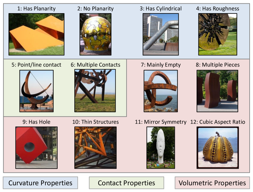
Figure 1: The 3D shape attributes investigated in this paper, and an illustration of each from our training set. Additional sample annotations are shown in Fig. 4.

Direct cues for higher order properties: One argument in favor of the direct approach is that many “cues for depth”, are actually direct cues for higher order properties, and thus converting them first into cues for depth is suboptimal. Examples include texture gradients [24, 12], which convey changes in surface orientation [20], or the curvature of occluding contours [38], which indicates the sign of the Gaussian curvature of the shape.

Resolution: Consider determining if a wire fence has thin structures or a piece of sandpaper has a rough surface. Compared to simply recognizing wires and bumps, the indirect method requires interpreting the scene at an incredibly detailed resolution – high enough to capture the pixels of the fence wire and sub-millimeter bumps on the sandpaper.

Ambiguity: Finally, ambiguities in depth may not be ambiguities for higher order properties, and prematurely resolving them in terms of depth is often the wrong thing to do. For instance, consider observing a surface and having three plausible hypotheses for its shape: convex ($z=x^{2}$), concave ($z=-x^{2}$), and flat ($z=0$). Suppose one is overwhelmingly confident ($>95\%$ chance) it is not flat but places equal chance on it being the other possibilities. Even though the surface is unambiguously not flat, the correct surface with regards to depth in both the $L_{1}$- and $L_{2}$-norm sense is a flat surface. If the ambiguity is resolved in depth, the resulting interpretation in terms of higher order properties is radically and incorrectly altered. Instead, if one directly asks whether the curvature is non-zero, the correct answer is obtained.

4 3D Attribute Vocabulary

Which 3D shape attributes should we model? We choose 12 attributes based on questions about three properties of historical interest to the vision community – curvature (how does the surface curve locally and globally?), ground contact (how does the shape touch the ground?), and volumetric occupancy (how does the shape take up space?).

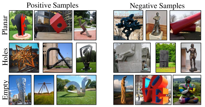
Figure 4: Sample positive and negative annotations from the dataset for the planar, has-holes, and empty attributes.

Fig. 1 illustrates the 12 attributes, and sample annotations are shown in Fig. 4. We now briefly describe the attributes in terms of curvature, contact, and volumetric occupancy.
Curvature Attributes: We take inspiration from a line of work on shape categorization via curvature led by Koenderink and van Doorn (e.g., [40]). Most sculptures have a mix of convex, concave, and saddle regions, so we analyze where curvature is zero in at least one direction and look for (1) Has Planarity: piecewise planar sculptures; (2) Has No Planarity: sculptures with no planar regions (note that many sculptures have a mix of planar and non-planar regions); (3) Has Cylindrical: sculptures where one principal curvature is zero (e.g., cylindrical ones); and (4) Has Roughness: rough sculptures where locally the surface changes rapidly.
Contact Attributes: Contact and support reasoning plays a strong role in scene understanding (e.g., [34, 28, 32, 63, 27]). We characterize ground contact via (5) Point/line Contact: point or line contact as compared to contact with the full body; (6) Multiple Contacts: whether multiple contacts between the object and the ground are made.
Volumetric Attributes: Reasoning about occupied-space has long been a goal of 3D understanding [32, 49, 58]. We ask (7) Mainly Empty: the fraction of occupied space in the sculpture; (8) Multiple Pieces: whether the sculpture has multiple pieces; (9) Has Hole: whether there are holes (i.e., the topology of the sculpture); (10) Has Thin Structures: whether it has thin structures, irrespective of whether they are sheets or tubular; (11) Mirror Symmetry: whether it is reflection symmetric i.e., if there is a plane of mirror symmetry in 3D; and (12) Cubic Aspect Ratio: whether it has a cubic aspect ratio in 3D.

Note that of the 12 attributes, 10 are relatively unaffected by a geometric affine transformation of the image (or 3D space) – only the mirror symmetry and cubic aspect ratio attributes are measuring a global metric property.

These are, of course, not a complete set. We do not model, for example, enclosure properties or differentiate a single large hole from a mesh. Similarly, many properties, such as Koenderink and Van Doorn’s shape index or Beiderman’s geons are localized or part-based. We leave this to future work.

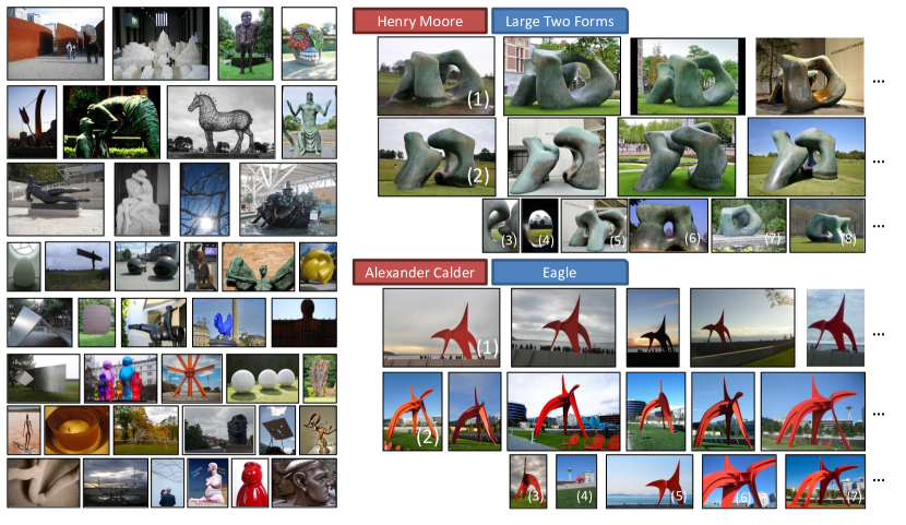
Figure 2: The dataset consists of 143K images of sculptures that were gathered from Flickr and Google images. A representative sample is shown on the left. Note the great variety in shape, material, and style. Our data has structure in terms of artist, work, and viewpoint cluster (shown numbered on the right). Each is important for investigating 3D shape attributes.

5 Gathering a Dataset of 3D Shapes

In order to investigate these 3D attributes, we need a dataset of 3D shapes that has a diversity of shape so that different subsets of attributes apply. We use modern sculptures as our source of 3D shapes since they are diverse in form and in-the-wild photos of them are available in great quantities on the Internet.

One alternative would be to use ordinary objects, such as the 20 PASCAL objects [15]. Unfortunately, ordinary objects have limited diversity, not just in terms of overall combinations of shape attributes, but also in terms of shape attributes conditioned on category. In practice, this means that if we set out to study shape with ordinary objects, our learning models may simply exploit categories as proxy variables: for example, rather than analyze planarity, our models may take the short-cut of distinguishing people from trains, then predicting planarity accordingly. In contrast, sculpture is free to depict people as planar or objects that defy categorization.

While using modern sculpture helps prevent a trivial solution, artists often produce work in a similar style: Alexander Calder’s sculptures are mostly piecewise planar, Constantin Brancusi’s egg-shaped, and Henry Moore’s are smooth and non-planar. We therefore need a variety of artists and multiple works/images of each. Previous sculpture datasets [2, 3] are not suitable for this task as they only contain a small number of artists and viewpoints.

Thus we gather a new dataset from Flickr. We adopt a five stage process to semi-automatically do this: (i) obtain a vocabulary of artists and works (for which many images will be available); (ii) cluster the works by viewpoint; (iii) clean up mistakes; (iv) query expand for more examples from Google images; and (v) label attributes. Note, organization by artist is not strictly necessary. However, artists are used subsequently to split the works into train and test datasets: as noted above, due to an artists’ style, shape attributes frequently correlate with an artist; consequently artists in the train and test splits must be disjoint to avoid an overly optimistic generalization performance. The statistics for these stages are given in Tab. I.

5.1 Generating a vocabulary of artists and works

Our goal is to generate a vocabulary of artists and works that is as broad as possible. We begin by producing a list of artists, combining manually generated lists with automatic ones, and then expand each artist to a list of their works.

The manual list consists of the artists exhibited at six sculpture parks picked from online top-10 lists, as well as those appearing in Wikipedia’s article on Modern Sculpture. An automatic list is generated from metadata from the 20 largest sculpture groups on Flickr: we analyze image titles for text indicating that a work is being ascribed to an artist, and take frequent bigrams and trigrams. The two lists are manually filtered to remove misspellings, painters and architects, a handful of mistakes, and artists with fewer than 250 results on Flickr. This yields 258 artists (95 from the manual list, and 163 from the automatic).

We now find a list of potential works for each artist using both Wikipedia and text analysis on Flickr. We query the sculptor’s page on Wikipedia, possibly manually disambiguating, and propose any italicized text in the main body of the article as a possible work. We also query Flickr for the artists’ works (e.g., Tony Smith Sculpture), and do n-gram analysis in titles and descriptions in front of phrases indicating attribution to the sculpture (e.g., “by Tony Smith”). In both cases, as in [57], stop-word lists were effective in filtering out noise. While Wikipedia has high precision, its recall is moderate at best and zero for most artists. Thus querying Flickr is crucial for obtaining high quality data. Finally, images are downloaded from Flickr for each work of each artist.

5.2 Building viewpoint clusters

TABLE I: Data statistics at each stage and the trainval/test splits.

Stage	Images	Artists	Works	View. Clusters
Initial	352K	258	3412	–
View Clust.	213K	246	2277	16K
Cleaned	97K	242	2197	9K
Query Exp.	143K	242	2197	9K
Trainval/Test	109K/35K	181/61	1655/532	7.2K/2.1K

Images from each work are partitioned into viewpoint clusters. These clusters are image sets that, for example, capture a different visual aspect of the work (e.g. from the front or side) or are acquired from a particular distance or scale (e.g. a close up). Fig. 2 shows example viewpoint clusters for several works.

There are two principal reasons for obtaining viewpoint clusters: (i) it enables recognition of a work from different viewpoints to be evaluated; and (ii) it makes label annotation more efficient as attributes are in general valid for all images of a cluster. Note, it might be thought that attributes could be labelled at the work level, but this is not always the case. For example, the hole in a Henry Moore sculpture or the ground contact of an Alexander Calder sculpture may not be visible in some viewpoint clusters, so those clusters will be labelled differently from the rest (i.e., no hole for the former, and unknown for the latter).

Clustering proceeds in a standard manner by defining a similarity matrix between image pairs, and using spectral clustering over the matrix. The pairwise similarity measure takes into account: (i) the number of correspondences (that there are a threshold number); (ii) the stability of these correspondences (using cyclic consistency as in [75]); and (iii) the viewpoint change (the rotation and aspect ratio change obtained from an affine transformation between the images). Computing correspondences requires some care though since sculptures often do not have texture (and thus SIFT like detections cannot be used). We follow [1] and first obtain a local boundary descriptor for the sculpture (by foreground-background segmentation and MCG [4] edges for the boundaries), and then obtain geometrically consistent correspondences using an affine fundamental matrix. Finally, a loose affine transformation is computed from the correspondences (loose because the sculpture may be non-planar, hence the earlier use of a fundamental matrix).

In general, this procedure produces clusters with high purity. The main failure is when an artist has several visually similar works (e.g. busts) that are confused in the meta-data used to download them. We also experimented with using GPS, but found the tags to be too coarse and noisy to define satisfactory viewpoint clusters.

5.3 Data Cleanup

The above processes are mainly automatic and consequently make some mistakes. A number of manual and semi-automatic post-processing steps are therefore applied to address the main failings. Note, we can quickly manipulate the dataset via viewpoint clusters as opposed to handling each and every image individually.

Cluster filtering: Each cluster is checked manually using three sample images to reject clearly impure clusters.

Regrouping: Some of the automatically generated works are ambiguous due to noisy meta-data: for instance “Reclining Figure” describes a number of Henry Moore sculptures. After clustering, these are reassigned to the correct works.

Outlier image removal: A 1-vs-rest SVM is trained for each work, using fc7 activations of a CNN [44] pretrained on ImageNet [59]. Each work’s images are sorted according to the SVM score, and the bottom images ($\approx 10K$ across all works) flagged for verification.

5.4 Expansion Via Search Engines

Figure 3: (a) Frequency of each attribute (i.e., # positives /# labeled); (b) Correlation between attributes.

Finally, we augment the dataset by querying Google. We perform queries with the artist and work name. Using the same CNN activation + SVM technique from the outlier removal stage, we re-sort the query results and add the top images after verification. This yields $\approx 45K$ more images.

5.5 Attribute Labeling

The final step is to label the images with attributes. Here, the viewpoint clusters are crucial, as they enable the labeling of multiple images at once. Each viewpoint cluster is labeled with each attribute, or can be labeled as N/A in case the attribute cannot be determined from the image (e.g., contact properties for a hanging sculpture). One difficulty is determining a threshold: few sculptures are only planar and no sculpture is fully empty. We assume an attribute is satisfied if it is true for a substantial fraction of the sculpture, typically 80%. To give a sense of attribute frequency, we show the fraction of positives in Fig. 3(a).

The dataset is also diverse in terms of combinations of attributes and inter-attribute correlation. There are $2^{12}=4096$ possible combinations, of which 393 occur in our data. Most attributes are uncorrelated according to the correlation coefficient $\phi$, as seen in Fig. 3(b): mean correlation is $\phi=0.13$ and $82\%$ of pairs have $\phi<0.2$. The two strong correlations ($\phi>0.5)$ are, unsurprisingly, (1) planarity and no planarity; and (2) emptiness and thinness.

6 Approach

We now describe the CNN architecture and loss functions that we use to learn the attribute predictors and shape embedding. We cast this as multi-task training and optimize directly for both. Specifically, the network is trained using a loss function over all attributes as well as an embedding loss that encourages instances of the same shape to have the same representation. The former lets us model the attributes that are currently labeled. The latter forces the network to learn a representation that can distinguish sculptures, implicitly modeling aspects of shape not currently labeled.

Network Architecture: We adapt the VGG-M architecture proposed in [11]. We depict the overall architecture in Fig. 5: all layers are shared through the last fully connected layer, fc7. After the 4096D fc7, the model splits into two branches, one for attributes, the other for embedding. The first is an affine map to $12$D followed by independent sigmoids, producing $12$ separate probabilities, one per attribute. The second projects fc7 to a $1024$D embedding which is then normalized to unit norm.

We directly optimize the network for both outputs, which allows us to obtain strong performance on both tasks. The first loss models all the attributes with a cross-entropy loss summed over the valid attributes. Suppose there are $N$ samples and $L$ attributes, each of which can be $1$ or $0$ as well as $\emptyset$ to indicate that the attribute is not labeled; the loss is

$$\small L(Y,P)=\sum_{i=1}^{N}\sum_{\begin{subarray}{c}l=1\\ Y_{i,l}\not=\emptyset\end{subarray}}^{L}Y_{i,l}\log(P_{i,l})+(1-Y_{i,l})\log(1-P_{i,l}),$$ (1)

for image $i$ and label $l$, where we denote the label matrix as $Y_{i,l}\in\{0,1,\emptyset\}^{N,L}$ and the predicted probabilities as $P_{i,l}\in[0,1]^{N,L}$. The second loss is an embedding loss over triplets as in [70, 60, 61]. Each triplet $i$ consists of an anchor view of one object $x_{i}^{a}$, another view of the same object $x_{i}^{p}$, as well as a view of a different object $x_{i}^{n}$. The loss aims to ensure that two images of the same object are closer in feature space compared to another object by a margin:

$$\sum_{i=1}\max\left(D(x_{i}^{a},x_{i}^{p})-D(x_{i}^{a},x_{i}^{n})+\alpha,0\right)$$ (2)

where $D(\cdot,\cdot)$ is squared Euclidean distance. We generate triplets in a mini-batch and use soft-margin violaters [60].

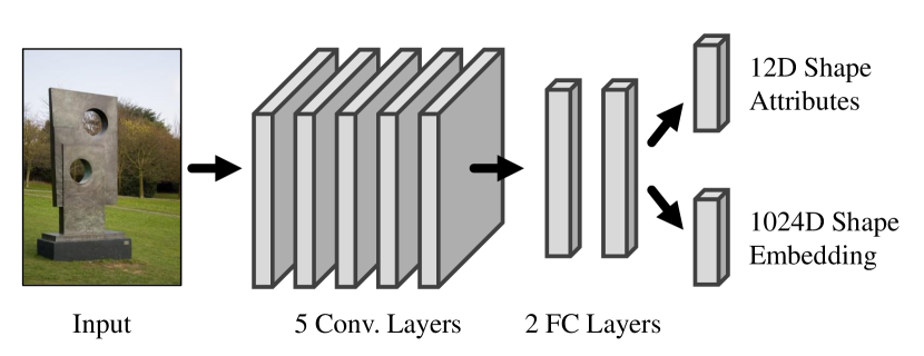
Figure 5: The multi-task network architecture, based on VGG-M. After shared layers, the network branches into layers specialized for attribute classification and shape embedding.

We see a number of advantages to multi-task learning. It yields a network that can both name attributes it knows about and model the 3D shape space implicitly. Additionally, we found it to improve learning stability, especially compared to individually modeling each attribute.

Configurations: We explore two configurations to validate that we are really learning about 3D shape. Unless otherwise specified, we use the system described above, Full. However, to probe what is being learned in one experiment, we also learn a network that only optimizes the attribute Loss (1), which we refer to as Attribute-Only.

Implementation Details: Optimization: We use a standard stochastic gradient descent plus momentum approach with a batch size of 128. We balance the two losses by multiplying the triplet loss by $3$, which was determined by optimizing each loss independently. Initialization: We initialize the network using the model from [11] which was pre-trained on image classification [59]. Parameters: We use a learning rate of $10^{-4}$ for the pre-trained layers, and $10^{-3}$ and $10^{-2}$ for classification and embedding layers respectively. We set the margin $\alpha$ to 0.1; we found that too-large margins led to poor optimization. Augmentation: At training time, we use random crops, flips, and color jitter. At test time, we sum-pool over multiple scales, crops and flips as in [11].

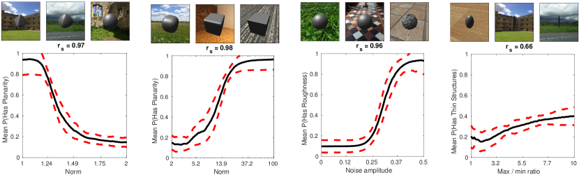
Figure 6: Plots of predicted attributes vs parameters. For each stimulus, we show a plot of the mean predicted shape attribute against the relevant parameter, sample images at the $10$th, $50$th, and $90$th percentiles of the parameter, and give the rank correlation. Red error bars indicate the standard deviation after centering the per-background responses at zero.

7 Analysis by Synthesizing Stimuli

Interpreting results on pre-captured in-the-wild data can be challenging because the cause of two images being interpreted differently could be due to any number of changes between the images. We therefore first analyze our results in a controlled setting, via synthetic data, where all underlying factors of an image are tightly controlled. Synthetic data offers an opportunity to systematically analyze a model’s behavior since it enables one to be sure that only one parameter changes between two images and to control that change. This technique was inspired by past work [77] that probed network response as a function of 2D patch transformations and simple variations, which in turn was inspired by human psychophysics. Here, we use a 3D graphics engine to generate the stimuli, and thus we can modulate properties of the underlying 3D shape as opposed to 2D transformations.

This approach is complementary to the more commonly used localization analysis such as [74, 64] (which we perform later in Section 8.2). In localization, the goal is to identify parts of a particular image that especially contribute to a final decision; interpreting these parts or activations is then done post-hoc by humans. Here, since all factors of variation can be exactly controlled, we can examine network response as a function of these factors. The primary disadvantage is that it requires a good synthetic model in which the factors of interest can be controlled. Nontheless, we see three compelling benefits to analysis by synthesizing stimuli: (a) it functions as a controlled experiment and can conclusively identify the factor responsible for a change in the data; (b) it can characterize subtle global changes, for instance the slight flattening of a sphere; and (c) it enables experiments that are practically impossible with real images, such as fixing shape and changing texture or creating hybrid stimuli that combine conflicting cues from two different shapes.

We begin by defining our stimuli, which consist of parameterized deformations of the unit-norm ball. We then test how well the network learned on sculpture can interpret these deformations, providing verification that the network has learned the properties of interest. Finally, having defined our stimuli and verified that they are being interpreted correctly, we analyze how sensitive our network is to various cues, using planarity as our property of interest due to the large literature on curvature perception (e.g., [7, 36, 40]). Our results show that the network is simultaneously incorporating a variety of signals ranging from mathematically-modelable shape cues such as shading and contours to data-driven correlations between shape, color, and texture.

7.1 Stimuli

We use three synthetic stimuli consisting of the deformation of a unit-norm ball; each stimuli is parameterized by a single parameter $p$: (i) $L_{p}$: the $L_{p}$ ball, $\{\mathbf{x}\in\mathbb{R}^{3}:||\mathbf{x}||_{p}=1\}$, i.e., $p=1$ is a octahedron, $p=2$ is a sphere, and $p=\infty$ is a cube. We split this stimulus into two stimuli to ensure a monotonic relationship between planarity and the parameter: a stimulus with $p\in[1,2]$, linearly spaced, and one with $p\in[2,100]$, logarithmically spaced. (ii) Noise: the unit sphere with the radius at each vertex additively displaced by a fixed noise pattern generated with fractal Brownian noise. We vary the magnitude of this noise $p\in[0,0.5]$. (iii) Oval: A sphere with the $X$ and $Z$ axes scaled by a factor $p\in[1,\frac{1}{10}]$. Each tests a different attribute: $L_{p}$ tests questions of planarity; Noise test questions of roughness; and Oval tests cubic aspect ratio and thinness.

Each geometry was generated with $\approx 90K$ vertices and then rendered with a gray specular material under a soft ambient light and a single directional light source using the code of [5]. Finally, each rendering was composited on top of 10 images of open spaces depicting indoor and outdoor spaces and no salient objects. We use multiple backgrounds to preclude effects due to any one particular background (e.g., inadvertent camouflaging).

7.2 Accuracy Experiments

After training the network described in Section 6, we first verify that the network can interpret these stimuli correctly. In addition to providing additional confirmation that the network has learned the actual properties, any subsequent analysis is useless unless the network interprets the stimuli correctly. We should note that this is not guaranteed: as [66] points out, there is a considerable domain shift between real and synthetic images.

Quantitative criteria: Our stimuli all satisfy the property that increasing a parameter $p$ increases the presence of an attribute in the shape. We can thus quantify performance by evaluating the correlation between attribute predictions and parameter $p$. Since the relationship is not necessarily linear, we use Spearman’s rank correlation $r_{s}$, which characterizes whether there is a monotonic relationship: $1$ indicates perfect rank correlation; $0$ indicates no correlation. Since the background alters the predicted attribute, we analyze per-background and report the average across backgrounds.

Results: We show a plot of the predicted shape attributes against the varied parameter $p$ in Fig. 6, as well as the rank correlation. The black line indicates the average across backgrounds. Directly computing the standard deviation across backgrounds mixes the actual uncertainty with a per-background bias that each background may introduce: the backgrounds with planar textures are viewed as more planar by the network, for instance. We thus compute an updated standard deviation after centering each background’s graph at zero and report $1$ standard deviation with a red error bar.

Despite the great dissimilarity between these stimuli and the data on which the model was trained, the network successfully generalizes well and a clear trend emerges in each case. If we repeat the analysis on all the backgrounds pooled together, this trend remains similar, and the rank correlations in each case decrease by an average of only $0.1$.

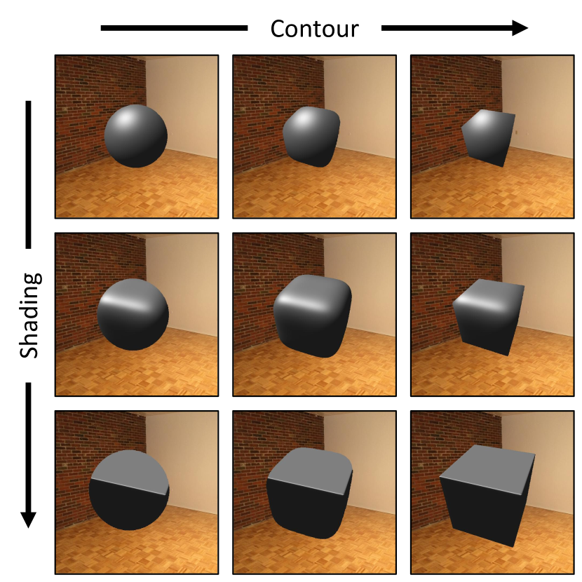
Figure 7: Examining the role of contour and shading cues in the output of the network. The contour and shading changes from sphere to cube going along the horizontal and vertical directions respectively. The network perceives stimuli closer to the bottom right as more planar.

7.3 Results with Conflicting Cues

There are a variety of cues by which people and machines can see 3D, so an important question is how the network is doing it. For instance: the results on PASCAL showed that a network trained on sculptures could accurately identify non-planar trains. It is not clear, however, what cues were used. Now that we have showed that the network interprets the stimuli correctly, we aim to address this question.

The synthetic stimuli let us analyze this question via composite objects that have conflicting cues, similar to cue combination techniques used in human subjects [10, 53, 52, 71]. Here, we use this to analyze the role of contour and shading cues in predicting the planarity of an object by creating objects that combine the contours and shading cues of a sphere and cube – for instance, a sphere that has the occluding contour of a cube. By shading, we mean the change in intensity caused by the projection of the light onto a particular shape. We show some examples of these objects in Fig. 7: each row or column depicts a fixed shading (row) or occluding contour (column); the original stimulus goes along the diagonal. In the original stimulus, the cues were varied jointly, but we can also fix one cue and vary the other.

TABLE II: How has planar surfaces changes as contour and shading vary or are held constant as a sphere or cube. Changing both cues simultaneously naturally causes the strongest response; changing each cue while holding the other constant causes a change; and varying shading produces a stronger response of the two cues.

Shading	Varying	Varying		Sphere	Cube
Contour	Varying	Sphere	Cube	Varying
$r_{s}$	0.98	0.96	0.97	0.50	0.36
Range	0.85	0.71	0.73	0.15	0.14

Results: Both cues are being used by the network, but shading cues appear to dominate contour ones. We quantify this by correlation and range of responses: if a cue is being used, the perceived planarity should be correlated with the change in cue (i.e., more planar contours produce more planar perceptions); the range of values taken when a cue is varied indicates how heavily the cue is used. We show both metrics in Table II in the case where we vary one or more cues. It can be seen that: both cues are used; the strongest response occurs when both are varied at the same time; and if only shading produces a far stronger response than contour. We also found that the contour cue was inconsistent in its effectiveness across backgrounds, presumably due to varying difficulty in finding the precise contour.

7.4 Sensitivity to Light

If shading cues are important for interpreting shape, then it may be sensitive to the lighting conditions. Here, we experimentally examine this with a set of 100 lighting setups. These have randomized count ($1$–$6$), locations, and colored intensities; results are similar with grayscale lighting, but lower variance in general.

Results: One way to evaluate how sensitive the network is to lighting is to quantify how lighting and predicted planarity vary together. For instance, ideally we ought to see the same strong correlation between underlying shape and predicted shape, even under extreme and unrealistic lighting. We find this to be true: for fixed background and lighting, there is still an average $0.9$ rank correlation between the predicted and actual shape; occasional failures happen with harsh overexposing lighting that obscures details. Similarly, if we fix the input stimulus, we ought to see little variance as we change the lighting. Unambiguous stimuli (octahedra/spheres/cubes) were interpreted consistently: the standard deviation across the lightings ranges from $0.06$ to $0.08$ on these stimuli (as reference the difference between the average cube and sphere interpretation is $0.7$). Ambiguous stimuli had a higher variance, but all had standard deviations below $0.21$.

An important case are catastrophic errors where lighting radically changes shape interpretation. We quantify this by examining how frequently octahedra and cubes were predicted as less planar than spheres. This never occurred when lighting was set identically for the stimuli. Changing lighting independently for the two stimuli cause mistakes in a handful ($37$) of cases out of the $200K$ possible pairs ($<0.02\%$). Most were caused by lighting hiding one stimulus and revealing the other (e.g., green light on one stimulus and deep purple on another, both in front of green hills).

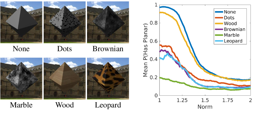
Figure 8: Texture variations and their effect on the perception of the $L_{p}$ stimulus. Marble-like texture changes the interpretation, although changing shape also changes the prediction irrespective of texture.

7.5 Sensitivity to Texture

We next examine whether the network has learned any correlations between texture and shape. We try six texture options: (1) None, the original material; (2) Dots, randomized ellipses; (3) Brownian, fractal Brownian noise; (4) Marble, which is the Brownian stimulus histogram equalized, which yields a marble-like effect; (5) Wood; and (6) Leopard print. Dots tests a simple synthetic stimuli; Brownian and Marble are useful since they are simple transformations of each other; Wood and Leopard test textures that are not simple mathematical processes.

Results: We show the six stimuli and the response curve, averaged over backgrounds, for each texture on the $L_{p}$, $p\in[1,2]$ stimulus in Figure 8. First, we note that, just as in the case of lighting variations, the network still produces the correct response to the stimulus for any particular texture: the average rank correlation between perceived geometry and underlying geometry is $0.96$. Second, the differences between the curves suggest that the network has learned to exploit correlations between texture and shape: for instance, simply histogram-equalizing the Brownian stimulus to make it look like marble changes the overall likelihood of planarity. This is presumably due to the fact that most marble statues are non-planar. Nonetheless, although texture modulates the planarity response, the actual shape continues to control it. This suggests that the network factors in natural correlations between texture and shape, but is not completely controlled by it.

7.6 Conclusions

In this section, we have made steps towards characterizing the behavior of a CNN trained to predict shape attributes via synthetic stimuli. In the process, we have provided evidence that the network is sensitive to the correct factors of variation and relatively insensitive to spurious signals such as lighting. Moreover, we have demonstrated that it uses classic cues to shape such as contours and shading but that it relies more on shading cues. Finally, we have demonstrated that the network has learned to exploit correlations between materials and shape

TABLE III: Area under the ROC curve. Higher is better. Our approach achieves strong performance and outperforms the baselines by a large margin.

	Curvature				Contact		Occupancy
Method	Plan	$\neg$ Plan	Cyl	Rough	P/L	Mult	Emp	Mult	Hole	Thin	Sym	Cubic		Mean
[6] + [9]	64.1	63.4	51.2	61.3	61.1	61.6	66.5	52.8	56.0	63.5	56.2	55.7		59.4
[14] + [9]	64.6	61.0	50.6	60.6	57.5	60.9	65.2	55.7	52.4	65.7	57.2	51.2		58.5
[6] + [29]	70.0	64.4	53.1	63.9	63.6	64.8	73.7	56.4	54.1	69.7	60.2	56.2		62.5
[14] + [29]	67.5	61.8	51.9	64.8	58.5	64.8	71.5	57.8	52.4	67.7	59.4	56.1		61.2
Proposed	82.8	77.2	56.9	76.0	74.4	76.4	87.0	60.4	69.3	85.8	60.8	60.3		72.3

8 Experiments

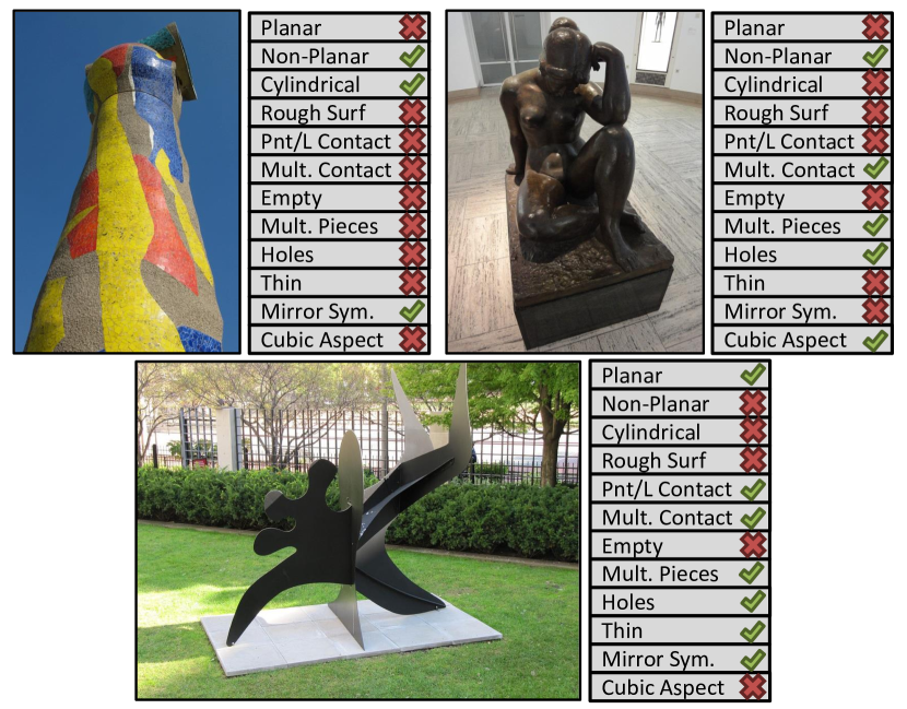
Figure 9: Thresholded predictions for all attributes on test images. The system has never seen these sculptures or ones by the artists who made them, but generalizes successfully.

Having analyzed the behavior of the network on synthetic data, we now evaluate it on our real data. We describe a set of experiments to investigate both the performance of the learnt 3D shape attribute classifiers, and what has been learnt. We aim to answer two basic questions in this section: (1) how well can we predict 3D shape attributes from a single image? and (2) are we actually predicting 3D properties or a proxy property that correlates with attributes in an image? To address (1) we evaluate the performance on the Sculpture Images Test set, and also compare to alternative approaches that first predict a metric 3D representation and then derive 3D attributes from that (Sec. 8.1). We probe (2) in a variety of ways. First, we examine the regions of the image responsible for the predictions in Sec 8.2. Second, we evaluate the learnt representation on a different task – determining if two images from different viewpoints are of the same object or not (Sec. 8.3). Third, we evaluate how well the 3D shape attributes trained on the Sculpture images generalize to non-sculpture data, in particular to predicting shape attributes on PASCAL VOC categories (Sec. 8.4). Finally, we probe the model with a set of synthetic stimuli in Section 7.

8.1 Attribute Prediction

We first evaluate how well 3D shape attributes can be estimated from images. Here, we report results for our full network. Since our dataset is large enough, the attribute-only network does similarly. We compare the approach proposed in this paper (which directly infers holistic attributes) to a number of baselines that are depth orientated, and start by computing a metric depth at every pixel.

Baselines: The baselines start by estimating a metric 3D map, and then attributes are extracted from this map. We use two recent methods for estimating depth from single images with code available: a CNN-based depth estimation technique [14] and an intrinsic images technique [6]. Since [6] expects a mask, we use the segmentation used for collecting the dataset (in Sec. 5.2). One question is: how do we convert these depthmaps into our attributes? Hand-designing a method is likely to produce poor results. We take a data-driven approach and treat it as a classification problem. We use two approaches that have produced strong performance in the past. The first is a linear SVM on top of kernel depth descriptors [9], which convert the depthmap into a high-dimensional vector incorporating depth configurations and image location. The second is the HHA scheme [29], which converts the depthmap into a representation amenable for fine-tuning a CNN; in this case, we learn the attribute CNN described in Section 6.

Evaluation Criteria: Each method produces a prediction scoring how much the image has the attribute. We characterize the predictive ability of these scores with a receiver operator characteristic (ROC) over the Sculpture images test set. This enables comparison across attributes since the ROC is unaffected by class frequency [18]. We summarize scores with the area under the ROC curve (AUROC).

Results: Fig. 9 shows thresholded predictions of all of the attributes on a few sculptures. To help visualize what has been learned, we show automatically sampled results in Fig. 10, sorted by the predicted presence of attributes.

We report quantitative results in Table III. On an absolute basis, certain attributes, such as planarity and emptiness, are easier than others to predict, as seen by their average performance; harder ones include ones based on symmetry and aspect ratio, which may require a global comparison across the image, as opposed to aggregation of local judgments.

In relative terms, our approach out-performs the baselines, with especially large gains on planarity, emptiness, and thinness. Note that reconstructing thin structures is challenging even with multi-view stereo as input and typically requires specialized handling [69]; an approach based on depth-prediction is thus likely to fail at reconstruction, and thus on attribute prediction. Instead, our system directly recognizes that the object is thin (e.g., Fig. 9 bottom). Fig. 10 shows that frequently, the instances that least have an attribute are the negation of the attribute: for example, even though many other sculptures are not rough, the least rough objects are especially smooth.

The system’s mistakes primarily occur on images where it is uncertain: sorting the images by attribute prediction and re-evaluating on the top and bottom 25% of the images yields a substantial increase to 77.9% mean AUROC; using the top and bottom $10\%$ yields an increase to 82.6%.

Throughout, we fix our base representation to VGG-M [11]. Switching to VGG-16 [65] gives an additional boost: the mean increases from 72.3 to 74.4 and $1/3$ of the attributes are predicted with AUROCS of $80\%$ or more.

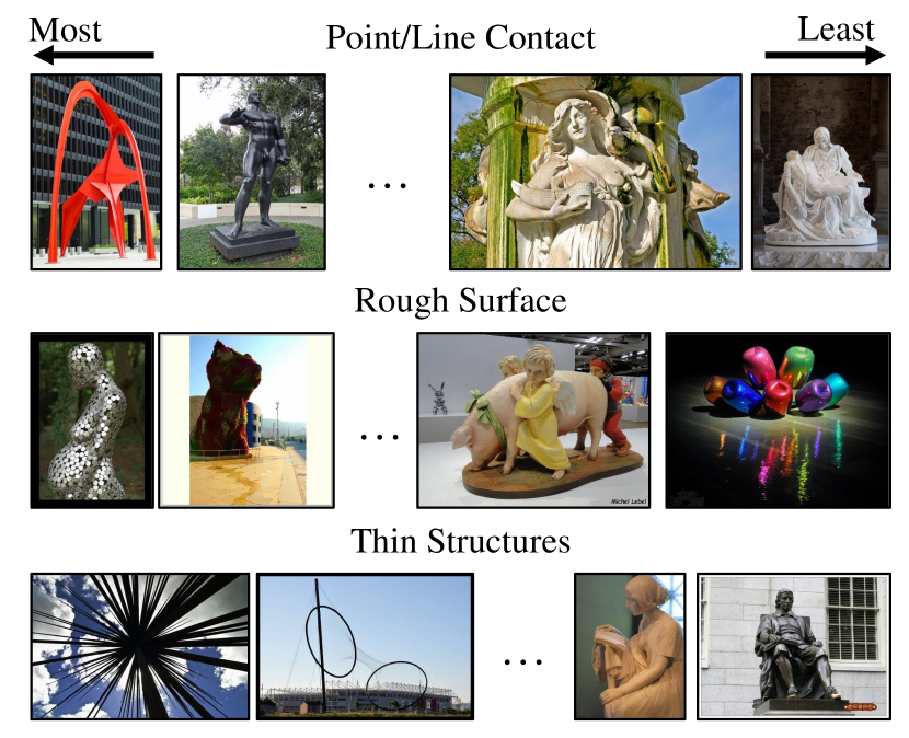
Figure 10: Test images sampled at the top, 95${}^{\textrm{th}}$, 5${}^{\textrm{th}}$ percentiles and lowest percentile with respect to three attributes.

8.2 Saliency Maps

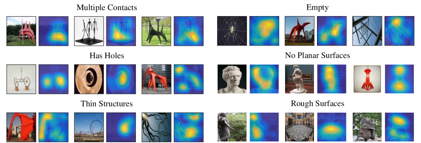
Figure 11: Class Activation Maps for six of the shape attributes. For each attribute, we select an image that the network predicts has high presence of an attribute (in top 1K scoring images) and overlay the class activation map for that attribute.

As a way of examining the network, we use the class-activation mapping (CAM) technique from [74].

Experimental Setup: Using the CAM technique involves connecting the last convolutional layer to the classification weights by average pooling, thus producing a final feature that has as many channels as the convolutional layer but $1\times 1$ spatial resolution. We thus remove both fully connected layers of our VGG-M network and attach an average pooling layer to the conv5 layer. Having done this, we retrain the network following identical settings.

It should be noted that this produces a different network. However, we found it makes similar decisions to the network trained in Section 8.1: the average correlation between the retrained and previous networks’ activations on the test set is high ($0.87$); the mean AUROC is slightly ($0.64\%$) lower (consistent with results reported for other architectures in [74]), and the maximum deviation of any attribute’s ROC is $3.9\%$.

Results: We examine saliency by looking at images in the images which cause the top $1$K strongest predictions for each attribute in the test set. Fig. 11 shows a selection of these for six attributes. The maps suggest that the network is using the right parts of the image to make its decision, even in the case of confident mistakes (Has Holes, right, which appears to be a hole due to an accidental viewpoint). In the case of analyzing contact, the network appears to be using the place at which “legs” of the sculpture split apart, and employs a similar strategy for the empty property. Roughness seems driven by rough surfaces, or, judging by the map on the set of stools, particular texture frequencies. We found that more global properties, such as mirror symmetry produce results that are more difficult to interpret.

Localization Results: We found that the CAM maps localized the sculpture well, suggesting that irrespective of which part is being used, the sculpture itself is driving predictions. To quantify this, we examined segmentation on a set of $40$ hand-segmented images. We treat the CAM maps as per-pixel predictions of whether the sculpture is in that pixel and evaluate the predictions by computing an AUROC on a per-pixel basis. Each CAM map produces at least a 71% AUROC; when normalized and averaged, they together achieve 85% AUROC.

8.3 Mental Rotation

If we have learned about 3D shape, our learnt representation ought to encode or embed 3D shape. But how do we characterize this embedding systematically? To answer this, we turn to the task of mental rotation [62, 67] which is the following: given two images, can we tell if they are different views of the same object or instead views of different objects? This is a classification task on the two presented images: for instance, in Fig. 12, the task is to tell that (a) and (b) correspond, and that (a) and (c) do not.

Note, the design of the dataset has tried to ensure that sculpture shape is not correlated with location by ensuring that images of a particular work come from different locations (since multiple instances of a work are produced) and different materials (e.g., bronze and stone in Fig. 12).

We report four representations: (i) the 1024D embedding produced by our full network; (ii) the 4096D fc7 layer of the full network; (iii) the 4096D fc7 layer of the attribute-only network; (iv) the attribute probabilities themselves from the full network. If our attribute network is using actual 3D properties, then the attribute network’s activations ought to work well for the mental rotation task even though it was never trained for it explicitly. Additionally, the attributes themselves ought to perform well.

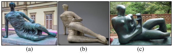
Figure 12: In mental rotation, the goal is to verify that (a) and (b) correspond and (a) and (c) do not. Roughness is a useful cue here.

Baselines: We compare our approach to (i) the pretrained FC7 from the initialization of the network and to (ii) IFV [56] over the BOB descriptor [2] that was used to create the dataset and dense SIFT [51]. The pre-trained FC7 characterizes what has been learned; the IFV representations help characterize the effectiveness of the attribute predictions on their own. We use the cosine distance throughout.

Evaluation Criteria: We adopt the evaluation protocol of [35] which has gained wide acceptance in face verification: given two images, we use their distance as a prediction of whether they are images of the same object or not. Performance is measured by AUROC, evaluated over 100 million of the pairs, of which $0.9\%$ are positives. Unlike [35], positives in the same viewpoint cluster are ignored: these are too easy decisions.

We further hone in on difficult examples by automatically finding and removing easy positives which can be identified with a bare minimum image representation. Specifically, we remove positive pairs with below-median distance in a 512-vocabulary bag-of-words over SIFT representation. This yields a more challenging dataset with $0.3\%$ positives. As mentioned in Sec. 5 artists often produce work of a similar style, and the most challenging examples are often pairs of images from the same artist (which may or may not be of the same work). We call the standard setting Easy and the filtered setting with only hard positives Hard.

Quantitative Results: Table IV and Fig. 13 show results for both settings. By themselves, the 12D attributes produce strong performance, 3-4% better than IFV representations. The attribute-only network improves over pretraining (by 0.9% in easy, 2.5% in hard), suggesting that it has learned the shape properties needed for the task. The full system does best and substantially better than any baseline (by 3.4% in easy, 6.9% in hard). This is to be expected since Equation 2, modulo a margin parameter, aims to ensure that any positive pair is closer than any negative pair, which is equivalent to the AUROC [18]. Relative performance compared to the initialization consistently improves for both the full system and the attribute-only system when going from Easy to Hard settings, providing further evidence that the system is indeed modeling 3D properties.

TABLE IV: AUROC for the mental-rotation task. Both variants of our approach substantially out-perform the baselines.

	Full Network			Attr. Only	Pretr.	IFV
	Emb.	FC7	Attr	FC7	FC7	[51]	[2]
All	92.3	90.7	81.9	89.8	88.9	78.0	74.4
Hard	86.9	84.1	76.4	82.5	80.0	57.3	61.9

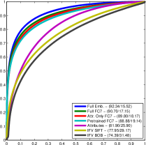
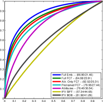
(a) Easy Setting	(b) Hard Setting

Figure 13: Mental rotation ROCs for easy and hard settings. In the legend, we report the AUROC and EER for each method.

Failure Modes: Examining incorrect pairs reveals a number of failure modes that suggest room for further improvement by future work. We define mistakes by converting distances in shape embedding space into classifications by thresholding at the equal error rate point. Figure 14 shows a few illustrative examples of these embedding mistakes; all of the false negatives (i.e., two views of the same sculptures that have high distance) depicted are further apart than all the false positives (i.e., two distinct sculptures that have low distance).

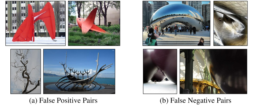
Figure 14: Examples of typical mental rotation failures. Every pair in (a) has lower distance in the embedding space than every pair in (b).

The two most frequent causes of false negative pairs are specular objects that reflect their surroundings and enormous objects that lend themselves to being photographed from a variety of different viewpoints. The most confused object, Anish Kapoor’s Cloud Gate (‘The Bean’) (Fig. 14(b) top) combines both of these. The remaining mistakes are pairs with dramatic scale or viewpoint changes, images where the sculpture is not the salient object, and a handful of labeling errors.

False positive pairs tend to be works by the same artist that or that are similar in terms of properties. The within-artist mistakes tended to be caused by a series of works with a common material and theme, for instance Alexander Calder’s works with red sheet metal (e.g., Fig. 14(a) top). Across artists, the network sometimes had difficulty distinguishing different sculptures made with thin metal structures and between statues of people.

Updated metadata: The above mental rotation experiments are done using the metadata from our prior work [21]. We have since updated the metadata and will release the updates. First, we manually identified works of art in the test set that are of similar shape (i.e., sharing the same attributes) but exactly the same subject (e.g., busts of animals from Ai Weiwei’s Zodiac Heads) and excluded them from mental rotation evaluation. We then trained a CNN on the entire dataset to discriminate between works. Confident prediction mistakes ($866$) were examined for reassignment frequently confused sculptures ($10$) were examined for merging or exclusion. In total $7$ works and $699$ images were updated. Evaluating on this cleaner data leads to an increase in AUROC of about $0.1\%$; the influence of these updates is limited since the metric is computed over pairs: the updates affect a small fraction of images and an even smaller number of pairs.

8.4 Object Characterization

Our evaluation has so far focused on sculptures, and one concern is that what we learn may not generalize to more everyday objects like trains or cats. We thus investigate our model’s beliefs about these objects by analyzing its activations on the PASCAL VOC dataset [15]. We feed the windows of the trainval set of VOC-2010 to our shape attribute model, excluding difficult and too-small ($<100$px) windows, and obtain a prediction of the probability of each attribute. We probe the representation by sorting class members by their activations (i.e., “which trains are planar?”) and sorting the classes by their mean activations.

Per-image results: The system forms sensible beliefs about the PASCAL objects, as we show in Fig. 15. Looking at intra-class activations, cats lying down are predicted to have single, non-point contact as compared to ones standing up; trains are generally planar, except for older cylindrical steam engines. Similarly, the non-planar dining tables are the result of occlusion by non-planar objects.

Per-category results: The system performs well at a category-level as well. Note that averaging over windows characterizes how objects appear in PASCAL VOC, not how they are prototypically imagined: e.g., as seen in Fig. 15, the cats and dogs of PASCAL are frequently lying down or truncated. The top 3 categories by planarity are bus, TV Monitor, train; and the bottom 3 are cow, horse, sheep. For point/line contact: bus, aeroplane, car are at the top and cat, bottle, sofa are at the bottom. Finally, sheep, bird, and potted plant are the roughest categories in PASCAL and car, bus, and aeroplane the smoothest.

Discriminating between classes: It ought to be possible to distinguish between the VOC categories based on their 3D properties, and thus we verify that the predicted 3D shape attributes carry class-discriminative information. We represent each window with its 12 attribute probabilities and train a random forest classifier for two outcomes in a 10-fold cross-validation setting: a 20-way multiclass model and a one-vs-rest. The multiclass model achieves an accuracy of 65%, substantially above chance. The one-vs-rest model achieves an average AUROC of 89%, with vehicles performing best.

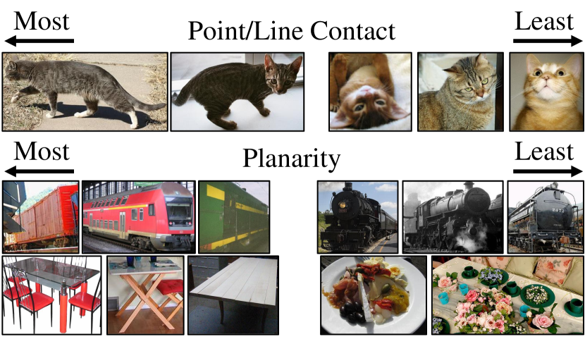
Figure 15: The top activations on PASCAL objects for Planarity and Point/Line Contact.

9 Summary and Extensions

We have shown that 3D shape attributes can be inferred directly from images at quite high quality. In the process, we have introduced a large dataset of modern sculpture for analyzing 3D shape attributes, verified that our learned models are actually inferring the attributes and not a proxy property and analyzed what cues are being used to infer these attributes.

One application is to use the attributes to help constrain metric reconstruction. There has been considerable work recently on using categories to constrain or regularize reconstruction [37, 47, 30] – for example roads and walls should be planar but people should not be – and 3D shape attributes can be used similarly. In contrast to categories, though, attributes offer a number of advantages: they can handle unseen categories, or the open world problem; they enable sharing across categories during learning; and they handle exceptions more easily – some walls and many roads are not, in fact, planar.

Another area of investigation is extending our shape attributes – for example, we did not consider changes in curvature, or the presence or absence of concavities. However, more generally, the attributes can be extended beyond absolute and global properties. Instead of absolute properties, many of our attributes (e.g., roughness) are better modeled as relative attributes. An alternative is to parse objects both globally as well as locally. For instance one could describe a sculpture as being primarily rough, but also localize any small smooth regions.

David F. Fouhey is a Postdoctoral Fellow at the Electrical Engineering and Computer Science Department, University of California, Berkeley.

Abhinav Gupta is an Assistant Professor at the Robotics Institute, Carnegie Mellon University.

Andrew Zisserman is the Professor of Computer Vision Engineering at the Department of Engineering Science, University of Oxford.

References

- [1] R. Arandjelović and A. Zisserman. Efficient image retrieval for 3D structures. In BMVC, 2010.
- [2] R. Arandjelović and A. Zisserman. Smooth object retrieval using a bag of boundaries. In ICCV, 2011.
- [3] R. Arandjelović and A. Zisserman. Name that sculpture. In ACM ICMR, 2012.
- [4] P. Arbeláez, J. Pont-Tuset, J. Barron, F. Marques, and J. Malik. Multiscale combinatorial grouping. In Computer Vision and Pattern Recognition, 2014.
- [5] M. Aubry, D. Maturana, A. A. Efros, B. Russell, and J. Sivic. Seeing 3D chairs: exemplar part-based 2D-3D alignment using a large dataset of CAD models. In CVPR, 2014.
- [6] J. T. Barron and J. Malik. Shape, illumination, and reflectance from shading. TPAMI, 2015.
- [7] I. Biederman. Recognition-by-components: A theory of human image understanding. Psychological Review, 94:115–147, 1987.
- [8] V. Blanz and T. Vetter. A morphable model for the synthesis of 3D faces. In SIGGRAPH, 1999.
- [9] L. Bo, X. Ren, and D. Fox. Depth Kernel Descriptors for Object Recognition. In IROS, 2011.
- [10] H. Bülthoff and H. Mallot. Integration of depth modules: stereo and shading. Journal of the Optical Society of America. A, Optics and image science, 5, 1989.
- [11] K. Chatfield, K. Simonyan, A. Vedaldi, and A. Zisserman. Return of the devil in the details: Delving deep into convolutional nets. In BMVC, 2014.
- [12] J. E. Cutting and P. M. Vishton. Perceiving layout and knowing distances: The interaction, relative potency, and contextual use of different information about depth. In W. Epstein and S. Rogers, editors, Perception of space and motion, pages 69–117, 1995.
- [13] D. Eigen and R. Fergus. Predicting depth, surface normals and semantic labels with a common multi-scale convolutional architecture. In ICCV, 2015.
- [14] D. Eigen, C. Puhrsch, and R. Fergus. Depth map prediction from a single image using a multi-scale deep network. In NIPS, 2014.
- [15] M. Everingham, L. Van Gool, C. K. I. Williams, J. Winn, and A. Zisserman. The PASCAL Visual Object Classes (VOC) challenge. IJCV, 88(2):303–338, 2010.
- [16] H. Fan, H. Su, and L. Guibas. A point set generation network for 3D object reconstruction from a single image. arXiv preprint arXiv:1612.00603, 2016.
- [17] A. Farhadi, I. Endres, D. Hoiem, and D. Forsyth. Describing objects by their attributes. In CVPR, 2009.
- [18] T. Fawcett. An introduction to ROC analysis. Pattern Recognition Letters, 27(8):861–874, June 2006.
- [19] V. Ferrari and A. Zisserman. Learning visual attributes. In NIPS, 2007.
- [20] D. Forsyth. Shape from texture and integrability. In ICCV, 2001.
- [21] D. Fouhey, A. Gupta, and A. Zisserman. 3D shape attributes. In CVPR, 2016.
- [22] D. F. Fouhey, A. Gupta, and M. Hebert. Data-driven 3D primitives for single image understanding. In ICCV, 2013.
- [23] D. F. Fouhey, A. Gupta, and M. Hebert. Unfolding an indoor origami world. In ECCV, 2014.
- [24] J. Gibson. Perception of the visual world. Houghton Mifflin, Boston, 1950.
- [25] R. Girdhar, D. Fouhey, M. Rodriguez, and A. Gupta. Learning a predictable and generative vector representation for objects. In ECCV, 2016.
- [26] B. Gong, J. Liu, X. Wang, and X. Tang. Learning semantic signatures for 3D object retrieval. IEEE Transactions on Multimedia, 15(2):369–377, 2013.
- [27] R. Guo and D. Hoiem. Support surface prediction in indoor scenes. In ICCV, 2013.
- [28] A. Gupta, A. Efros, and M. Hebert. Blocks world revisited: Image understanding using qualitative geometry and mechanics. In ECCV, 2010.
- [29] S. Gupta, R. Girshick, P. Arbelaez, and J. Malik. Learning rich features from RGB-D images for object detection and segmentation. In ECCV, 2014.
- [30] C. Häne, N. Savinov, and M. Pollefeys. Class specific 3d object shape priors using surface normals. In CVPR, 2014.
- [31] V. Hedau, D. Hoiem, and D. Forsyth. Recovering the spatial layout of cluttered rooms. In ICCV, 2009.
- [32] V. Hedau, D. Hoiem, and D. Forsyth. Recovering free space of indoor scenes from a single image. In CVPR, 2012.
- [33] D. Hoiem, A. Efros, and M. Hebert. Geometric context from a single image. In ICCV, 2005.
- [34] D. Hoiem, A. Efros, and M. Hebert. Putting objects in perspective. IJCV, 2008.
- [35] G. B. Huang, M. Ramesh, T. Berg, and E. Learned-Miller. Labeled faces in the wild: A database for studying face recognition in unconstrained environments. Technical Report 07-49, University of Massachusetts, Amherst, October 2007.
- [36] A. Johnston and P. J. Passmore. Independent encoding of surface orientation and surface curvature. Vision Research, 34(22):3005 – 3012, 1994.
- [37] A. Kar, S. Tulsiani, J. Carreira, and J. Malik. Category-specific object reconstruction from a single image. In CVPR, 2015.
- [38] J. J. Koenderink. What does the occluding contour tell us about solid shape? Perception, 13:321–330, 1984.
- [39] J. J. Koenderink. Solid Shape. MIT, 1990.
- [40] J. J. Koenderink and A. J. van Doorn. Surface shape and curvature scales. Image and Vision Computing, 10(8):557 – 564, 1992.
- [41] J. J. Koenderink and A. J. Van Doorn. Relief: Pictorial and otherwise. Image and Vision Computing, 13(5):321–334, 1995.
- [42] J. J. Koenderink, A. J. Van Doorn, and A. M. Kappers. Surface perception in pictures. Perception & Psychophysics, 52(5):487–496, 1992.
- [43] J. J. Koenderink, A. J. Van Doorn, and A. M. Kappers. Pictorial surface attitude and local depth comparisons. Perception & Psychophysics, 58(2), 1996.
- [44] A. Krizhevsky, I. Sutskever, and G. E. Hinton. Imagenet classification with deep convolutional neural networks. In NIPS, 2012.
- [45] N. Kumar, A. Berg, P. Belhumeur, and S. K. Nayar. Attribute and simile classifiers for face verification. In ICCV, 2009.
- [46] L. Ladický, J. Shi, and M. Pollefeys. Pulling things out of perspective. In CVPR, 2014.
- [47] L. Ladicky, P. Sturgess, C. Russell, S. Sengupta, Y. Bastanlar, W. Clocksin, and P. H. Torr. Joint optimisation for object class segmentation and dense stereo reconstruction. International Journal of Computer Vision, BMVC special award issue, 2011.
- [48] C. H. Lampert, H. Nickisch, and S. Harmeling. Learning to detect unseen object classes by between-class attribute transfer. In CVPR, pages 951–958, 2009.
- [49] D. C. Lee, A. Gupta, M. Hebert, and T. Kanade. Estimating spatial layout of rooms using volumetric reasoning about objects and surfaces. In NIPS, 2010.
- [50] D. C. Lee, M. Hebert, and T. Kanade. Geometric reasoning for single image structure recovery. In CVPR, 2009.
- [51] D. Lowe. Distinctive Image Features from Scale-Invariant Keypoints. IJCV, 60(2):91–110, 2004.
- [52] C. Madison, W. Thompson, D. Kersten, P. Shirley, and B. Smits. Use of interreflection and shadow for surface contact. Perception & Psychophysics, 63(2):187–194, 2001.
- [53] J. F. Norman and J. T. Todd. The perception of 3-D structure from contradictory optical patterns. Perception & Psychophysics, 57(6):826–834, 1995.
- [54] J. F. Norman and J. T. Todd. The discriminability of local surface structure. Perception, 25(4):381–398, 1996.
- [55] D. Parikh and K. Grauman. Relative attributes. In ICCV, 2011.
- [56] F. Perronnin, J. Sanchez, and T. Mensink. Improving the fisher kernel for large-scale image classification. In ECCV, 2010.
- [57] T. Quack, B. Leibe, and L. Van Gool. World-scale mining of objects and events from community photo collections. In CVIR, 2008.
- [58] J. Rock, T. Gupta, J. Thorsen, J. Gwak, D. Shin, and D. Hoiem. Completing 3D object shape from one depth image. In CVPR, 2015.
- [59] O. Russakovsky, J. Deng, H. Su, J. Krause, S. Satheesh, S. Ma, Z. Huang, A. Karpathy, A. Khosla, M. Bernstein, A. C. Berg, and L. Fei-Fei. ImageNet Large Scale Visual Recognition Challenge. IJCV, pages 1–42, April 2015.
- [60] F. Schroff, D. Kalenichenko, and J. Philbin. Facenet: A unified embedding for face recognition and clustering. In CVPR, 2015.
- [61] M. Schultz and T. Joachims. Learning a distance metric from relative comparisons. In NIPS, 2004.
- [62] R. N. Shepard and J. Metzler. Mental rotation of three-dimensional objects. Science, 171:701–703, 1971.
- [63] N. Silberman, D. Hoiem, P. Kohli, and R. Fergus. Indoor segmentation and support inference from RGBD images. In ECCV, 2012.
- [64] K. Simonyan, A. Vedaldi, and A. Zisserman. Deep inside convolutional networks: Visualising image classification models and saliency maps. In Workshop at International Conference on Learning Representations, 2014.
- [65] K. Simonyan and A. Zisserman. Very deep convolutional networks for large-scale image recognition. CoRR, abs/1409.1556, 2014.
- [66] H. Su, C. R. Qi, Y. Li, and L. J. Guibas. Render for CNN: Viewpoint estimation in images using cnns trained with rendered 3D model views. In ICCV, 2015.
- [67] M. J. Tarr and H. H. Bülthoff. Image-based object recognition in man, monkey and machine. Cognition, 67(1–2):1 – 20, 1998.
- [68] S. Tulsiani, T. Zhou, A. A. Efros, and J. Malik. Multi-view supervision for single-view reconstruction via differentiable ray consistency. In CVPR, 2017.
- [69] B. Ummenhofer and T. Brox. Point-based 3D reconstruction of thin objects. In ICCV, 2013.
- [70] X. Wang and A. Gupta. Unsupervised learning of visual representations using videos. In ICCV, 2015.
- [71] A. E. Welchman, A. Deubelius, V. Conrad, H. H. Bülthoff, and Z. Kourtzi. 3D shape perception from combined depth cues in human visual cortex. Nature neuroscience, 8(6):820–827, 2005.
- [72] J. Wu, C. Zhang, T. Xue, B. Freeman, and J. Tenenbaum. Learning a probabilistic latent space of object shapes via 3D generative-adversarial modeling. In NIPS, pages 82–90, 2016.
- [73] X. Yan, J. Yang, E. Yumer, Y. Guo, and H. Lee. Perspective transformer nets: Learning single-view 3D object reconstruction without 3D supervision. In NIPS, 2016.
- [74] B. Zhou, A. Khosla, A. Lapedriza, A. Oliva, and A. Torralba. Learning deep features for discriminative localization. In CVPR, 2016.
- [75] T. Zhou, Y. J. Lee, S. X. Yu, and A. A. Efros. Flowweb: Joint image set alignment by weaving consistent, pixel-wise correspondences. In CVPR, 2015.
- [76] A. Zisserman, P. Giblin, and A. Blake. The information available to a moving observer from specularities. Image and Vision Computing, 7(1):38–42, 1989.
- [77] D. Zoran, P. Isola, K. Krishnan, and W. Freeman. Learning ordinal relationships for mid-level vision. In ICCV, 2015.