Angular decay coefficients of $J/\psi$ mesons at forward rapidity from $p$$+$$p$ collisions at $\sqrt{s}=510$ GeV

Abstract

We report the first measurement of the full angular distribution for inclusive $J/\psi\rightarrow\mu^{+}\mu^{-}$ decays in $p$$+$$p$ collisions at $\sqrt{s}=510$ GeV. The measurements are made for $J/\psi$ transverse momentum $2<p_{T}<10$ GeV/$c$ and rapidity $1.2<y<2.2$ in the Helicity, Collins-Soper, and Gottfried-Jackson reference frames. In all frames the polar coefficient $\lambda_{\theta}$ is strongly negative at low $p_{T}$ and becomes close to zero at high $p_{T}$, while the azimuthal coefficient $\lambda_{\phi}$ is close to zero at low $p_{T}$, and becomes slightly negative at higher $p_{T}$. The frame-independent coefficient $\tilde{\lambda}$ is strongly negative at all $p_{T}$ in all frames. The data are compared to the theoretical predictions provided by nonrelativistic quantum chromodynamics models.

I Introduction

Measurements of heavy quark bound states provide a unique opportunity to explore basic quantum chromodynamics (QCD). Because the energy scale of the heavy quark mass is larger than the hadronization scale, nonrelativistic QCD (NRQCD) techniques can be applied to provide theoretical access to hadronization. Charmonium, the bound state of a charm and anti-charm quark, is an especially convenient laboratory as it decays with a considerable branching fraction into two leptons. It is composed of two moderately heavy quarks, and is more copiously available than bottomonium (a bottom and anti-bottom bound state).

The charmonium wave function can be expressed as a combination of intermediate state contributions formed during the $c-\bar{c}$ hadronization stage. The S-wave charmonium wave function can be calculated from an expansion in a series of the charm and anti-charm velocity $\nu$ in the charmonium rest frame Bodwin et al. (1995),

$$\left|\psi_{Q}\right> = \mbox{$\mathcal{O}$}(1)\left|{}^{3}S_{1}^{(1)}\right>+\mbox{$\mathcal{O}$}(\nu)\left|{}^{3}P_{J}^{(8)}g\right>$$

$$+ \mbox{$\mathcal{O}$}\left(\nu^{2}\right)\left|{}^{3}S_{1}^{(8)}gg\right>+\mbox{$\mathcal{O}$}\left(\nu^{2}\right)\left|{}^{3}S_{0}^{(8)}g\right>+\cdots,$$

in the spectroscopic notation ${}^{2S+1}L_{J}$. The series contains color singlet⁽¹⁾ and color octet⁽⁸⁾ states. The nonrelativistic operators $\mathcal{O}$ are parametrized from experimental results.

Several models have been proposed for the production of $J/\psi$ mesons, each one with a different interpretation of these intermediate states. The Color Evaporation Model (CEM) Fritzsch (1977), applied only to hadronic collisions, assumes that the nonrelativistic amplitude is constant from twice the charm quark mass to twice the D meson mass and zero elsewhere. All relativistic diagrams to a fixed order in $\alpha_{s}$ producing a charm and anti-charm quark in the final state are included. The original Color-Singlet Model (CSM) Baier and Ruckl (1981) explicitly requires the $c\bar{c}$ pair produced in the hard scattering to be on-shell and in the same quantum state as the hadronized $J/\psi$ (${}^{2S+1}L_{J}=$${}^{3}S_{1}$). The nonrelativistic amplitude is taken as the real-space $J/\psi$ wave function evaluated at the origin. Early calculations of the CSM at LO in $\alpha_{s}$ under-predicted cross sections at CDF Abe et al. (1997) and PHENIX Adare et al. (2007). Recent calculations at next-to-leading order (NLO) Artoisenet et al. (2009); Chang et al. (2009) and next-to-next-to-leading order (NNLO) Artoisenet et al. (2008) increase the predicted cross section. NRQCD calculations Bodwin et al. (1995) predict nonnegligible contributions from $c\bar{c}$ production in the color-octet configuration, leading to a larger cross section and better agreement with data than the current CSM calculations.

Several terms in Eq. I produce similar $J/\psi$ cross sections and transverse momentum behavior, but can be experimentally distinguished because of their different helicities. The angular distribution of spin $\frac{1}{2}$ lepton decays from a spin 1 quarkonium state is derived from the density matrix $\rho_{m^{\prime}m}$ (where $m^{\prime}$ and $m$ have the possible values –1,0,1) of the production process and parity conservation constraints Jacob and Wick (1959); Collins and Soper (1977); Gottfried and Jackson (1964).

The elements of the matrix are identified as

$$\begin{array}[]{lllr}W_{L}&=&\rho_{00}&\textrm{(longitudinal helicity)}\\ W_{T}&=&\rho_{11}-\rho_{-1-1}&\textrm{(transverse helicity)}\\ W_{\Delta}&=&\frac{1}{\sqrt{2}}\left(\rho_{10}+\rho_{01}\right)&\textrm{(single spin-flip)}\\ W_{\Delta\Delta}&=&\rho_{1-1}&\textrm{(double spin-flip)}\end{array}$$ (2)

The angular distribution of the positive lepton from the $J/\psi$ decay can be written as

$$\begin{split}&\frac{dN}{d\cos\theta d\phi}\propto\\ &1+\lambda_{\theta}\cos^{2}\theta+\lambda_{\theta\phi}\sin 2\theta\cos\phi+\lambda_{\phi}\sin^{2}\theta\cos 2\phi\end{split}$$ (3)

where,

$$\begin{aligned} \lambda_{\theta~{}}&=&\frac{W_{T}-W_{L}}{W_{T}+W_{L}}\\ \lambda_{\phi~{}}&=&\frac{2W_{\Delta\Delta}}{W_{T}+W_{L}}\\ \lambda_{\theta\phi}&=&\frac{\sqrt{2}W_{\Delta}}{W_{T}+W_{L}}\end{aligned}$$

which we call the polar ($\lambda_{\theta}$), the azimuthal ($\lambda_{\phi}$) and the “mixed” ($\lambda_{\theta\phi}$) angular decay coefficients.

The angles $\phi$ and $\theta$ are measured relative to a reference frame defined such that the $\hat{x}$ and $\hat{z}$-axes lie in the production plane, formed by the momenta of the colliding protons and the particle produced. The direction of the $\hat{z}$-axis within the production plane is arbitrary. The simplest frame to study the particle wave function is the one in which the density matrix has only diagonal elements, or the single and double spin-flip terms are zero. This simplest frame is also called the natural frame and is identified when the azimuthal coefficients in (3) are zero. The three most common frames used in particle angular distribution studies are (Fig. 1):

The Helicity frame (HX)

Jacob and Wick (1959), traditionally used in collider experiments, takes the $\hat{z}$-axis as the spin-1 particle momentum direction.

The Collins-Soper frame (CS)

Collins and Soper (1977), widely used in Drell-Yan measurements, chooses the $\hat{z}$-axis as the difference between the momenta of the colliding partons boosted into the spin-1 particle rest frame. Note that while the original paper Collins and Soper (1977) and subsequent theoretical studies used colliding parton momenta in their calculations, the colliding hadron momenta are used here, because we do not have information about the parton momenta.

The Gottfried-Jackson frame (GJ)

Gottfried and Jackson (1964), typically used in fixed target experiments, takes the $\hat{z}$-axis as the beam momentum boosted into the spin-1 particle rest frame. At forward angles in a collider environment, the definition of the GJ frame depends heavily on which beam is used in the definition. If the beam circulating in the same direction as the $J/\psi$ momentum is chosen (GJ forward), the resulting $\hat{z}$-axis is nearly collinear with the $\hat{z}$-axis of the HX and CS frames and points in the same direction. In GJ backward frame (beam circulating in the direction opposite to $J/\psi$ momentum is chosen) the $\hat{z}$-axis points in the opposite direction.

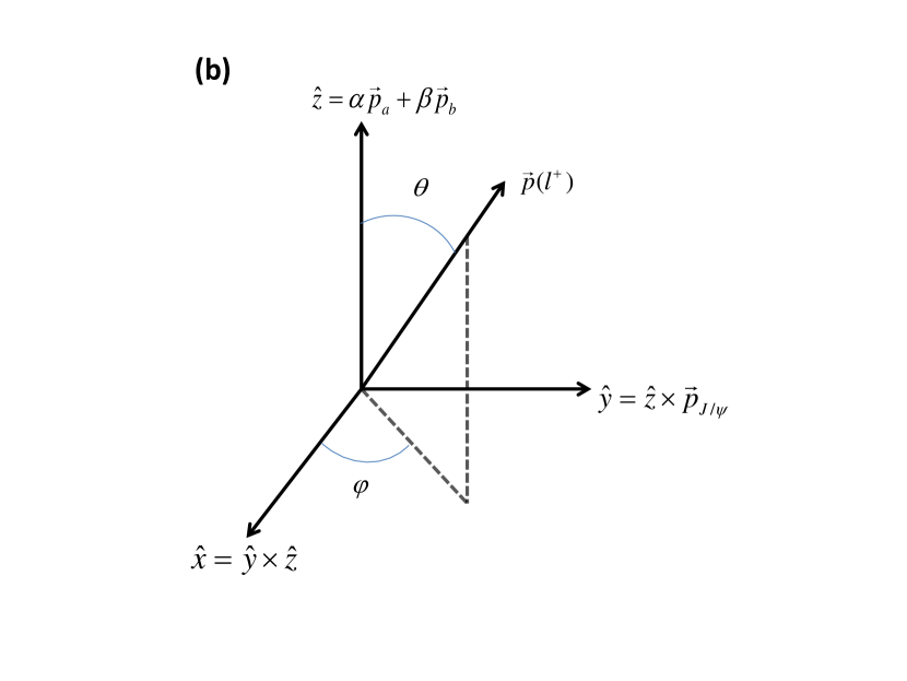
Figure 1: Reference frames and coordinate system used in this analysis. The $\hat{x}$ and $\hat{z}$-axes are chosen to lie in the production plane determined by the colliding hadrons and the particle produced (a $J/\psi$ in this figure). (a) shows the production plane and the direction convention for the $\hat{z}$ in the Collins-Soper (CS), Helicity (HX) and Gottfried-Jackson (GJ) reference frames. $\vec{p}_{a}$, $\vec{p}_{b}$ in this diagram, represent colliding parton momenta. Note that in an experiment we do not know parton momenta and use colliding hadron momenta instead. In (b) the angles $\theta$ and $\phi$ represent the direction of the positive decay lepton in the corresponding reference frame.

While the angular decay coefficients depend heavily on the reference frame, it was noted in Faccioli et al. (2009) that the $\lambda_{\theta}$ coefficient from various measurements transformed into the CS frames changes smoothly from longitudinal (negative) to transverse (positive) with increasing $J/\psi$ momentum. The smooth variation occurs between measurements from fixed targets by E866/NuSea Chang et al. (2003) and HERA-B Abt et al. (2009), as well as a collider environment by CDF Abulencia et al. (2007). The transformation of the measurements depends on the assumption that the $\hat{z}$-axis of the CS frame is the natural frame, along which the $J/\psi$ spin-alignment is purely longitudinal or transverse. The assumption is based on measurements of the angular distribution for inclusive $J/\psi$ decays from fixed target $p+N$ collisions at HERA-B covering $p_{T}<5$ GeV/$c$ and $-0.3<x_{F}<0.1$ Abt et al. (2009). It has been predicted that the natural frame at large $p_{T}$ is near to but not identically along the CS $\hat{z}$-axis Braaten et al. (2009). Subsequent work reported in Faccioli et al. (2010) obtained equations which could convert the angular parameters measured in one frame to another frame rotated around the $\hat{y}$-axis. A combination of polar and azimuthal constants can be arranged to form a frame-invariant angular decay coefficient

$$\widetilde{\lambda}=\frac{\lambda_{\theta}+3\lambda_{\phi}}{1-\lambda_{\phi}}.$$ (4)

$\widetilde{\lambda}$ is sensitive to the maximum angular asymmetry, or polarization, independent of the $\hat{z}$-axis orientation of the reference frame. A comparison between $\widetilde{\lambda}$ derived from the azimuthal coefficients measured in the different reference frames can be used as a consistency check of the parameters extracted from the various reference frames.

While there is no clear prediction for the $J/\psi$ spin-alignment from the CEM, it has been suggested that multiple soft gluon exchanges destroy the spin-alignment of the $c\bar{c}$ pair Amundson et al. (1997). Recent calculations at NLO Artoisenet et al. (2009); Chang et al. (2009) and NNLO Artoisenet et al. (2008) in the CSM improve agreement with the spin-alignment measured previously at PHENIX Adare et al. (2010), which is predicted at NLO to be longitudinal in the HX frame for large $p_{T}$ Lansberg (2011). Numerical estimates Beneke and Kramer (1997); Braaten et al. (2000) in the NRQCD approach and recent calculations at NLO Gong et al. (2009) predict a transverse spin-alignment in the HX frame at $p_{T}$ $\gg M_{J/\psi}$ due to gluon fragmentation, which disagrees in both sign and magnitude with data from CDF Abulencia et al. (2007). Measurements of the $J/\psi$ spin alignment in different kinematic regions can help distinguish the dominant production mechanism.

The PHENIX experiment has already published Adare et al. (2010) a $\lambda_{\theta}$ measurement for $J/\psi$’s produced in $p$$+$$p$ collisions at $\sqrt{s}=$ 200 GeV at midrapidity. In this paper we present a more comprehensive measurement of the full angular distributions for the leptonic decays of inclusive $J/\psi$ in $p$$+$$p$ collisions at $\sqrt{s}=$ 510 GeV for the HX, CS, GJ forward, and GJ backward reference frames. The measurement covers a transverse momentum range $2<p_{T}<10$ GeV/$c$ and rapidity range $1.2<y<2.2$.

The experimental apparatus used to measure dimuon pairs from $J/\psi$ decays is described in Section II. The procedure followed to obtain angular decay coefficients and their uncertainties is explained in Section III. The results, their comparison to other measurements and theoretical predictions are presented in Section IV.

II Experimental Setup and $J/\psi$ Selection

The measurements were carried out using the PHENIX detector Adcox et al. (2003) with data from $p$$+$$p$ collisions at $\sqrt{s}=510$ GeV recorded in 2013. Decays of $J/\psi$ $\rightarrow\mu^{+}\mu^{-}$ were measured in the muon spectrometer Akikawa et al. (2003) for $1.2<y<2.2$ and full azimuthal angle. Collisions are identified by triggering on a minimal multiplicity of hits in two beam-beam counters (BBC) Allen et al. (2003) placed at $3.0<|\eta|<3.9$. The data presented correspond to an integrated luminosity of 222 pb^-1. Approximately $117\times 10^{3}J/\psi$ mesons are used to determine the decay coefficients.

The PHENIX muon spectrometer comprises three finely-segmented multi-plane cathode strip tracking chambers (MuTr) located in a radial magnetic field and positioned in front of five layers of Iarocci tubes interleaved with thick steel absorbers (MuID), which provide a hadron rejection of $10^{-4}$. Events containing $J/\psi$ mesons are triggered using logical units composed of all tubes in a window projecting from the vertex through the MuID. To satisfy the trigger, trigger logic units in the horizontal and vertical projection must contain at least one hit in either the first or second layer of the MuID, one additional hit in either the fourth or fifth layer, and at least three hits in total. To avoid the low-momentum region where the trigger efficiency changes quickly before reaching a plateau, the muons used in this analysis are required to have momentum along the beam direction $p_{z}>$1.45 GeV/$c$ as measured at the first MuTr station for the spectrometer, corresponding to $\sim$2.1 GeV/$c$ at the vertex.

Events are required to occur within 30 cm of the center of the experimental apparatus along the beam direction as measured by the beam-beam counters. To improve hadron rejection, a fit of the two tracks to the collision vertex was performed and required to have $\chi^{2}<5$ per degree of freedom. MuTr tracks and MuID hit roads were required to match within four standard deviations to ensure that they correspond to the same particle.

III Analysis Procedure

In this section, we outline the procedure used to tune the simulation to data and extract both the shape of the $J/\psi$ yield and the angular decay coefficients.

III.1 $J/\psi$ Reconstruction

The $J/\psi$ mesons are reconstructed by calculating the invariant mass of all unlike-sign muon pairs after analysis cuts. Combinatorial random background is estimated by like-sign dimuons calculated as $2\sqrt{N^{++}N^{--}}$, where $N^{++}$ and $N^{--}$ are number of positive and negative same-sign pairs respectively, and subtracted. Mass distributions for each bin in $p_{T}$ and rapidity are then fit using a double Gaussian as signal and exponential background to remove dimuons from Drell-Yan and correlated open-heavy flavor decays (see Fig. 2). The number of $J/\psi$’s is obtained directly by integrating the dimuon invariant mass distribution in a mass interval from 2.5 to 3.7 GeV/$c^{2}$ after background subtraction. Background subtraction was performed for each individual $\cos\theta$-$\phi$ bin (see Section III.3).

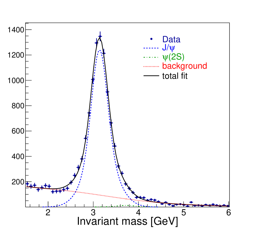
Figure 2: An example of the invariant mass distribution of oppositely charged dimuon pairs after like-sign background subtraction (dark blue points) fit with a double Gaussian for the $J/\psi$ (dashed blue curve) and $\psi(2S)$ (green dash-dotted curve) signals plus exponential for the background (dotted red curve). The solid black curve is the sum of signal and background fit.

III.2 Experimental Acceptance and Simulation Tuning

A simulation of $J/\psi$ mesons generated by tuned pythia 6.421 Sjostrand et al. (2001) is performed to determine the effects of the detector acceptance. As a complete geant 3 GEA (1993) model of the detector is used to obtain the efficiency and acceptance corrections in this analysis, the simulation itself needs to be well tuned to reproduce both low-level detector-related quantities and high level kinematic distributions. In particular, because we perform a two-dimensional fit to the data in $\cos\theta$-$\phi$ space for each reference frame, the inefficiencies in the experimental acceptance must be properly represented.

To ensure that the acceptance is approximately constant throughout the data-taking period, we excluded from analysis the data taken during time intervals when the MuTr or MuID had additional tripped high voltage channels over normal operation, or there were problems with data transmission from the detectors for $>$1% of all events. Areas of the detectors that were disabled or highly inefficient are eliminated in both the analyzed data and simulations. In addition, for the MuTr, the charges deposited in individual strips within a MuTr cluster are smeared in the simulation to match the measured properties in the data.

An example of the excellent agreement between tuned simulations and data for the MuTr is shown in Fig. 3, where cluster charge distributions in data and simulation are compared. In addition to the low-level performance of the MuTr, the MuID detector has an efficiency for pairs of Iarocci tubes that is a function of the collision rate seen by the BBC, varying between 0.93 at 400 kHz to 0.88 at 2.2 MHz. The mean efficiency over the course of the running period is used as the efficiency of each pair, as a uniform change in efficiency will not affect the relative angular acceptance.

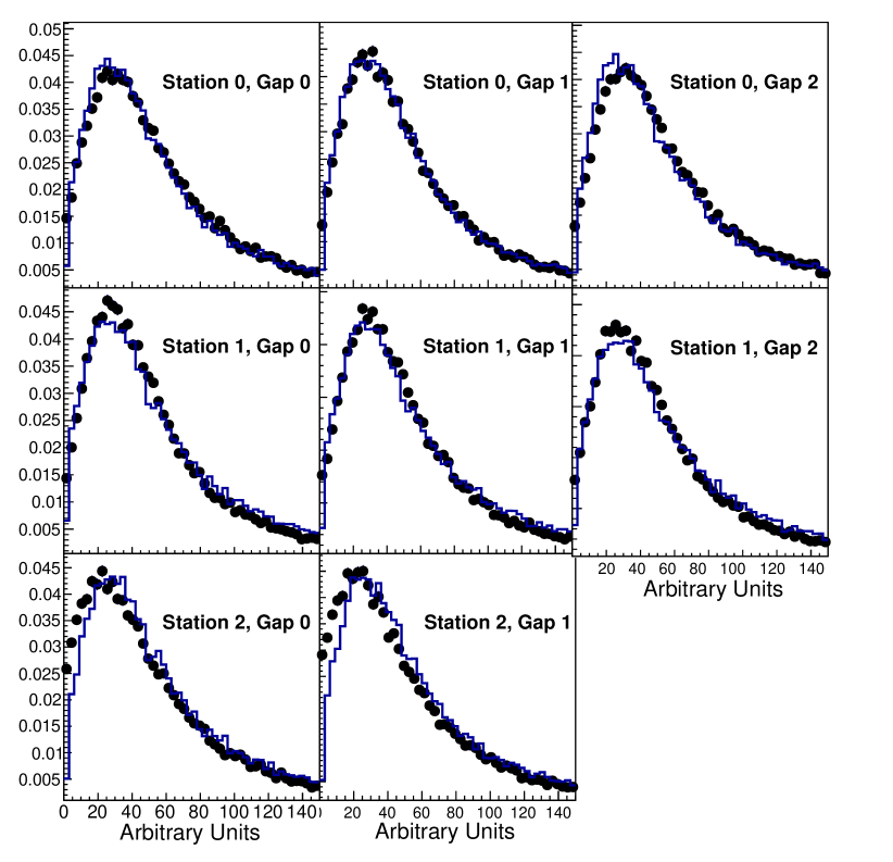
Figure 3: A comparison of the total cluster charge distributions in the MuTr in simulation (blue histogram) and data (closed black circles). Each MuTr station is composed of three (Stations 1 and 2) or two (Station 3) measurement planes (“gaps”) Akikawa et al. (2003). A cluster is the collection of ionization energy from the passage of a charged particle in the measurement plane.

At a higher level, a good match of simulation to the data is demonstrated in Fig. 4, where the mass resolution for simulated and reconstructed $J/\psi$’s is compared.

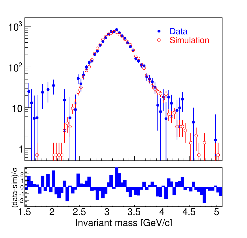
Figure 4: Invariant mass distribution of simulated $J/\psi$ (red open circles), and $J/\psi$’s reconstructed in data (solid blue dots) after all backgrounds are subtracted. The insert at the bottom shows (data-simulation)/$\sigma$ difference, where $\sigma$ is the statistical uncertainty of the difference.

Single unpolarized $J/\psi$’s were generated by pythia and processed through full geant simulation. Even after the tuning described at the beginning of this chapter, small additional $p_{T}$ and rapidity weights were still required to match the $J/\psi$’s $p_{T}$ and rapidity distributions in pythia to those measured experimentally. A systematic uncertainty, correlated between data points, was introduced to account for a possible mismatch between the $p_{T}$ and rapidity distributions in simulation and data. This systematic uncertainty was estimated by varying the $p_{T}$ and rapidity weights in simulation by 10%, or one standard deviation of the fits to the data (see Section III.4 for details). Because the detector acceptance in the simulation is sensitive to the input asymmetry in the decay muon distributions, the final step in the simulation was to apply angular decay coefficients obtained in the initial iteration as weights in the simulation, thus imitating the observed $J/\psi$ polarization.

The relative acceptance as a function of $p_{T}$ for the different reference frames is shown in Fig. 5.

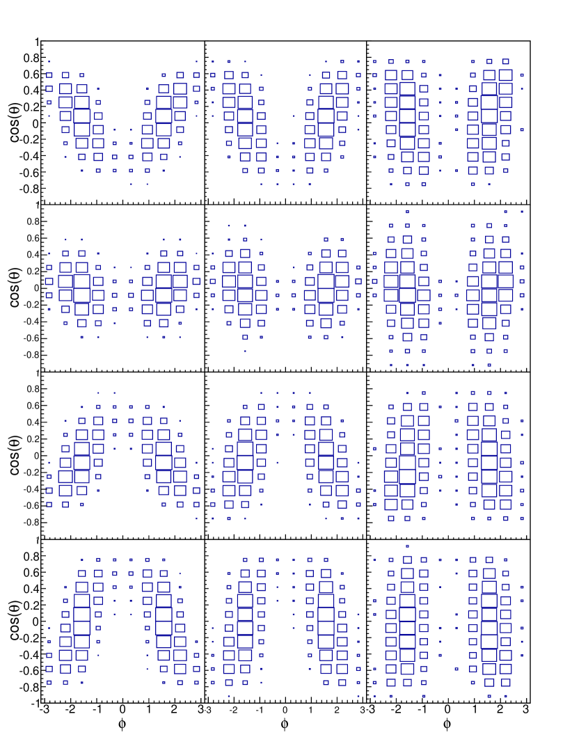
Figure 5: Relative acceptance in $\cos\theta$-$\phi$ bins in (from top to bottom) the HX, CS, GJ Backward, and GJ Forward frames for increasing $p_{T}$ from left to right. The area of rectangles is proportional to acceptance value in linear scale. See Section III.3 for definition of $p_{T}$, $\cos\theta$, and $\phi$ bins.

III.3 Angular Decay Coefficients

To extract the angular decay coefficients, the background subtracted $J/\psi$ yields are histogrammed according to the angular distribution of the positive muon in twelve bins of $\cos\theta$ by ten bins of $\phi$, and three bins in $p_{T}$ (2–3, 3–4, and 4–10 GeV$/c$) for each reference frame. The mean $p_{T}$ for each bin are 2.47, 3.46, and 5.45 GeV$/c$, respectively. The experimental data are corrected for acceptance, and then fit with Eq. 3. The fit is performed simultaneously in $\cos\theta$ and $\phi$ to extract all three angular decay coefficients $\lambda_{\theta}$, $\lambda_{\theta\phi}$, $\lambda_{\phi}$, and frame-independent $\widetilde{\lambda}$. In general the fits to the data are good, with a typical $\chi^{2}$ value per degree of freedom between 1.2-2.1, with the number of degrees of freedom typically in the 40–60 range.

The exact fitting procedure is outlined below.

1. The $J/\psi$ angular distributions are divided into 12 bins in $\cos{\theta}$ and 10 bins in $\phi$. Combinatorial and correlated background is subtracted bin-by-bin, and angular distributions are then corrected for acceptance, which is calculated assuming no polarization, that is $\lambda_{\theta}=\lambda_{\theta\phi}=\lambda_{\phi}=0$. This is done for each of the three transverse momentum bins in each polarization frame.

2. $\lambda_{\theta},\lambda_{\theta\phi}$, and $\lambda_{\phi}$ in Eq. 3 are varied separately and independently from $-1$ to $1$ with a $0.01$ step, and for each step a fit is done to the acceptance corrected measured angular distribution. The fit is done for a fixed value of all $\lambda$’s. The only free parameter is absolute normalization. A $\chi^{2}$ of the fit is calculated at each step. The minimum $\chi^{2}$ obtained in the three dimensional phase space spanned by $\lambda_{\theta}$, $\lambda_{\theta\phi}$ and $\lambda_{\phi}$ is chosen as the best fit.

3. Extracted $\lambda$ coefficients are used as weights in the simulation to generate acceptance for polarized $J/\psi$ which is used in the next iteration. Convergence is achieved when the newly extracted $\lambda$ coefficients become zero within the experimental uncertainty, which means that the polarization in the simulation matches that in the data.

The resulting angular decay coefficients $\lambda_{\theta}$, $\lambda_{\theta\phi}$, $\lambda_{\phi}$, and frame-independent coefficient $\tilde{\lambda}$ are shown in Fig. 9, Fig. 9, Fig. 9, and Fig. 9 respectively, for four reference frames as a function of transverse momentum.

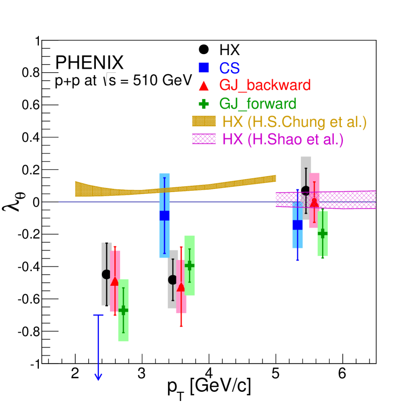
Figure 6: Polar angular decay coefficient $\lambda_{\theta}$ as a function of transverse momentum for four reference frames and three $p_{T}$ bins. Black circles: HX frame; blue squares: CS frame; red triangles: GJ Backward; green crosses: GJ Forward frames. Shaded error boxes show systematic uncertainty. Points are shifted in $p_{T}$ for clarity. Down-pointing arrow indicates 90% confidence level upper limit. The data are compared with NRQCD theoretical predictions in Helicity frame by H. S. Chung et al. Chung et al. (2011) and H. Shao et al. Shao et al. .

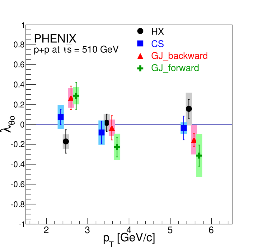
Figure 7: “Mixed” angular decay coefficient $\lambda_{\theta\phi}$ as a function of transverse momentum for four reference frames and three $p_{T}$ bins. Black circles: HX frame; blue squares: CS frame; red triangles: GJ Backward; green crosses: GJ Forward frames. Shaded error boxes show systematic uncertainty. Points are shifted in $p_{T}$ for clarity.

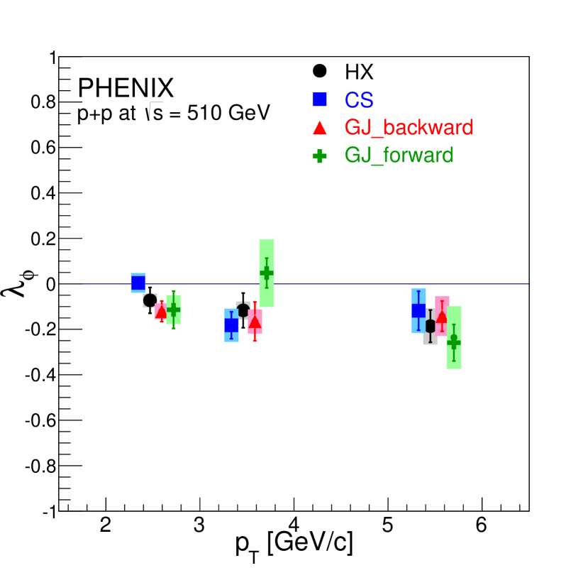
Figure 8: Azimuthal angular decay coefficient $\lambda_{\phi}$ as a function of transverse momentum for four reference frames and three $p_{T}$ bins. Black circles: HX frame; blue squares: CS frame; red triangles: GJ Backward; green crosses: GJ Forward frames. Shaded error boxes show systematic uncertainty. Points are shifted in $p_{T}$ for clarity.

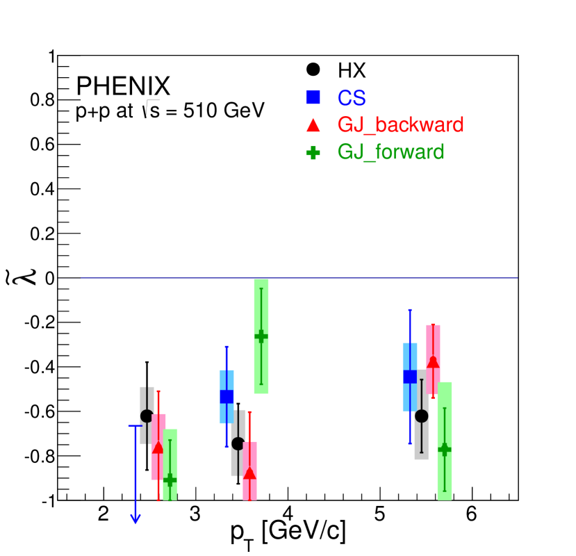
Figure 9: Frame-independent angular decay coefficient $\tilde{\lambda}$ as a function of transverse momentum for the four reference frames and three $p_{T}$ bins. Black circles: HX frame; blue squares: CS frame; red triangles: GJ Backward; green crosses: GJ Forward frames. Shaded error boxes show systematic uncertainty. Points are shifted in $p_{T}$ for clarity. Down pointing arrow indicates 90% confidence level upper limit.

III.4 Systematic Uncertainty Discussion

The statistical uncertainties of the angular decay coefficients were calculated by randomizing each bin in $\cos\theta$ vs. $\phi$ histograms with a Gaussian random number according to the statistical uncertainty in that bin, and re-fitting. This procedure was repeated one hundred times, and the RMS of the resulting $\lambda$ distribution was taken as a statistical uncertainty.

A measurement of the angular decay coefficients is sensitive to several factors, including the input $p_{T}$ and rapidity distribution in the simulation, exact matching of acceptance between data and simulation, how well the simulation reproduces low-level detector-related quantities, and time-varying conditions. These uncertainties were estimated by introducing variations in the input $p_{T}$ and rapidity distributions, fiducial cuts, and low-level deposited charge smearing in the simulation. Additional cross-checks included variations of the collision vertex cut and $J/\psi$ rapidity cut. Possible polarization bias in acceptance was studied with a simulation-based blind analysis. In this blind analysis simulated $J/\psi$’s generated with a certain polarization were used as fake data. A full analysis of the fake data was performed without prior knowledge of the input polarization, polarization coefficients were extracted and compared to the input values.

The resulting variations in angular decay coefficients were accounted for as systematic uncertainties and are listed in Table 1.

Table 1: Systematic uncertainties in the polarization measurement.

			$\lambda_{\theta}$			$\tilde{\lambda}$			$\lambda_{\phi}$			$\lambda_{\theta\phi}$
$p_{T}$ bin [GeV/$c$]:		2–3	3–4	4–10	2–3	3–4	4–10	2–3	3–4	4–10	2–3	3–4	4–10
HX	Acceptance	0.134	0.118	0.103	0.082	0.082	0.075	0.010	0.024	0.034	0.052	0.077	0.076
	Kinematics	${}^{+0.049}_{-0.023}$	${}^{+0.050}_{-0.008}$	${}^{+0.120}_{-0.038}$	${}^{+0.036}_{-0.004}$	${}^{+0.042}_{-0.001}$	${}^{+0.089}_{-0.049}$	${}^{+0.006}_{-0.009}$	${}^{+0.002}_{-0.004}$	${}^{+0.021}_{-0.028}$	${}^{+0.003}_{-0.012}$	${}^{+0.014}_{-0.010}$	${}^{+0.012}_{-0.043}$
	Hit smearing	0.134	0.131	0.140	0.094	0.119	0.173	0.027	0.031	0.067	0.050	0.035	0.142
	Polarization bias	0.015	0.010	0.005	0.016	0.011	0.006	0.002	0.002	0.001	0.010	0.008	0.005
	TOTAL	${}^{+0.196}_{-0.191}$	${}^{+0.183}_{-0.176}$	${}^{+0.211}_{-0.178}$	${}^{+0.130}_{-0.125}$	${}^{+0.150}_{-0.144}$	${}^{+0.209}_{-0.195}$	${}^{+0.030}_{-0.031}$	${}^{+0.039}_{-0.039}$	${}^{+0.079}_{-0.081}$	${}^{+0.072}_{-0.073}$	${}^{+0.086}_{-0.085}$	${}^{+0.162}_{-0.167}$
CS	Acceptance	0.106	0.148	0.079	0.076	0.101	0.083	0.010	0.010	0.025	0.061	0.076	0.042
	Kinematics	${}^{+0.011}_{-0.004}$	${}^{+0.020}_{-0.014}$	${}^{+0.061}_{-0.066}$	${}^{+0.0147}_{-0.006}$	${}^{+0.014}_{-0.016}$	${}^{+0.068}_{-0.074}$	${}^{+0.003}_{-0.001}$	${}^{+0.001}_{-0.004}$	${}^{+0.020}_{-0.020}$	${}^{+0.016}_{-0.015}$	${}^{+0.011}_{-0.025}$	${}^{+0.019}_{-0.025}$
	Hit smearing	0.085	0.214	0.099	0.045	0.061	0.107	0.042	0.072	0.092	0.102	0.092	0.032
	Polarization bias	0.016	0.012	0.006	0.017	0.013	0.007	0.002	0.002	0.0015	0.011	0.009	0.007
	TOTAL	${}^{+0.136}_{-0.136}$	${}^{+0.261}_{-0.261}$	${}^{+0.141}_{-0.143}$	${}^{+0.089}_{-0.088}$	${}^{+0.118}_{-0.119}$	${}^{+0.151}_{-0.154}$	${}^{+0.043}_{-0.043}$	${}^{+0.073}_{-0.073}$	${}^{+0.098}_{-0.098}$	${}^{+0.120}_{-0.120}$	${}^{+0.120}_{-0.122}$	${}^{+0.057}_{-0.059}$
GJB	Acceptance	0.111	0.138	0.081	0.086	0.106	0.089	0.012	0.013	0.026	0.065	0.071	0.045
	Kinematics	${}^{+0.013}_{-0.037}$	${}^{+0.021}_{-0.003}$	${}^{+0.106}_{-0.064}$	${}^{+0.005}_{-0.018}$	${}^{+0.029}_{-0.019}$	${}^{+0.075}_{-0.033}$	${}^{+0.010}_{-0.009}$	${}^{+0.007}_{-0.015}$	${}^{+0.013}_{-0.005}$	${}^{+0.013}_{-0.008}$	${}^{+0.013}_{-0.019}$	${}^{+0.054}_{-0.037}$
	Hit smearing	0.149	0.087	0.121	0.119	0.082	0.112	0.032	0.050	0.083	0.074	0.041	0.133
	Polarization bias	0.018	0.009	0.004	0.019	0.010	0.005	0.002	0.002	0.002	0.016	0.009	0.005
	TOTAL	${}^{+0.186}_{-0.189}$	${}^{+0.165}_{-0.163}$	${}^{+0.180}_{-0.159}$	${}^{+0.147}_{-0.148}$	${}^{+0.137}_{-0.136}$	${}^{+0.162}_{-0.147}$	${}^{+0.035}_{-0.035}$	${}^{+0.052}_{-0.054}$	${}^{+0.088}_{-0.087}$	${}^{+0.099}_{-0.098}$	${}^{+0.083}_{-0.084}$	${}^{+0.151}_{-0.145}$
GJF	Acceptance	0.129	0.122	0.120	0.081	0.084	0.078	0.015	0.026	0.035	0.061	0.076	0.074
	Kinematics	${}^{+0.005}_{-0.000}$	${}^{+0.024}_{-0.020}$	${}^{+0.008}_{-0.020}$	${}^{+0.029}_{-0.019}$	${}^{+0.007}_{-0.006}$	${}^{+0.096}_{-0.013}$	${}^{+0.017}_{-0.009}$	${}^{+0.006}_{-0.016}$	${}^{+0.112}_{-0.002}$	${}^{+0.022}_{-0.016}$	${}^{+0.023}_{-0.000}$	${}^{+0.044}_{-0.026}$
	Hit smearing	0.141	0.137	0.067	0.212	0.243	0.276	0.060	0.145	0.110	0.058	0.106	0.200
	Polarization bias	0.015	0.012	0.006	0.016	0.013	0.007	0.002	0.001	0.001	0.013	0.010	0.007
	TOTAL	${}^{+0.192}_{-0.191}$	${}^{+0.185}_{-0.184}$	${}^{+0.137}_{-0.139}$	${}^{+0.229}_{-0.227}$	${}^{+0.257}_{-0.257}$	${}^{+0.303}_{-0.287}$	${}^{+0.064}_{-0.063}$	${}^{+0.148}_{-0.149}$	${}^{+0.160}_{-0.115}$	${}^{+0.087}_{-0.086}$	${}^{+0.133}_{-0.131}$	${}^{+0.217}_{-0.214}$

Table 2: $\lambda_{\theta}$ and $\tilde{\lambda}$ in four frames. Only statistical errors are shown. Mean $p_{T}$ for each of the three bins are 2.47, 3.46, and 5.45 GeV/$c$ respectively. The numbers in the CS frame for the $p_{T}=2$–3 GeV/$c$ bin are 90% confidence level upper limits.

		$\lambda_{\theta}$			$\tilde{\lambda}$
$p_{T}$ bin [GeV/$c$]:	2–3	3–4	4–10	2–3	3–4	4–10
HX	-0.449 $\pm$ 0.195	-0.482 $\pm$ 0.131	0.069 $\pm$ 0.142	-0.621 $\pm$ 0.241	-0.745 $\pm$ 0.180	-0.621 $\pm$ 0.163
CS	<-0.701	-0.085 $\pm$ 0.238	-0.143 $\pm$ 0.221	<-0.665	-0.534 $\pm$ 0.221	-0.445 $\pm$ 0.305
GJB	-0.489 $\pm$ 0.218	-0.524 $\pm$ 0.252	-0.002 $\pm$ 0.134	-0.760 $\pm$ 0.256	-0.875 $\pm$ 0.279	-0.375 $\pm$ 0.171
GJF	-0.670 $\pm$ 0.141	-0.394 $\pm$ 0.105	-0.195 $\pm$ 0.151	-0.909 $\pm$ 0.185	-0.263 $\pm$ 0.221	-0.772 $\pm$ 0.190

Table 3: $\lambda_{\phi}$ and $\lambda_{\theta\phi}$ in four frames. Only statistical errors are shown. Mean $p_{T}$ for each of the three bins are 2.47, 3.46, and 5.45 GeV/$c$ respectively.

		$\lambda_{\phi}$			$\lambda_{\theta\phi}$
$p_{T}$ bin [GeV/$c$]:	2–3	3–4	4–10	2–3	3–4	4–10
HX	-0.073 $\pm$ 0.057	-0.117 $\pm$ 0.077	-0.186 $\pm$ 0.071	-0.171 $\pm$ 0.120	0.016 $\pm$ 0.087	0.157 $\pm$ 0.094
CS	0.004 $\pm$ 0.027	-0.182 $\pm$ 0.059	-0.118 $\pm$ 0.086	0.075 $\pm$ 0.076	-0.081 $\pm$ 0.110	-0.035 $\pm$ 0.120
GJB	-0.121 $\pm$ 0.045	-0.165 $\pm$ 0.085	-0.142 $\pm$ 0.067	0.267 $\pm$ 0.120	-0.034 $\pm$ 0.120	-0.156 $\pm$ 0.063
GJF	-0.114 $\pm$ 0.082	0.048 $\pm$ 0.065	-0.259 $\pm$ 0.080	0.288 $\pm$ 0.140	-0.230 $\pm$ 0.100	-0.313 $\pm$ 0.110

The total systematic uncertainty shown as shaded boxes in Figs. 9 through 9 is taken to be the quadratic sum of these components, assuming that they are uncorrelated.

IV Results and Discussion

We have presented the first measurement of the full angular distribution from $J/\psi$ decays to muons in $p$$+$$p$ collisions at $\sqrt{s}$ = 510 GeV at forward rapidity ($1.2<y<2.2$) in the Helicity, Collins-Soper, and Gottfried-Jackson reference frames. The results are summarized in Tables 2 and 3, and in Figs. 9 through 9.

The measurements presented here are for inclusive $J/\psi$. Feed-down from higher mass quarkonium states also contribute to the observed polarization and is not separated out.

In all frames the polar coefficient $\lambda_{\theta}$ is strongly negative at low $p_{T}$ and becomes close to zero at high $p_{T}$, while the azimuthal coefficient $\lambda_{\phi}$ is close to zero at low $p_{T}$, and becomes slightly negative at higher $p_{T}$. The frame-independent coefficient $\tilde{\lambda}$ is strongly negative at all $p_{T}$ in all frames. Consistency of $\tilde{\lambda}$ values in all polarization frames indicates that systematic uncertainties are well under control. The obtained polarization coefficient $\tilde{\lambda}$ is in good agreement with what was reported by the STAR experiment Trzeciak (2015), for the same $\sqrt{s}$ at midrapidity and higher transverse momentum.

At the Large Hadron Collider (LHC), the LHCb experiment Aaij et al. (2013) reported similar, although smaller values of $\lambda_{\theta}$ with similar trend in transverse momentum at forward rapidity. $\lambda_{\theta}$ measured by the ALICE experiment Abelev et al. (2012) at forward rapidity is consistent with no polarization, although, within experimental uncertainty, it can be said to be similar to the LHCb result. A very comprehensive CMS measurement Chatrchyan et al. (2013) indicates that both $\lambda_{\theta}$ and $\tilde{\lambda}$ are consistent with zero. However, note that the CMS measurement covers much a higher transverse momentum range and for more central rapidities.

The measured polar coefficient $\lambda_{\theta}$ is compared to theoretical prediction for prompt $J/\psi$ in Helicity frame calculated in the NRQCD factorization approach by H. S. Chung et al. Chung et al. (2011) and H. Shao Shao et al. in Fig. 9. At high transverse momentum both predictions are in good agreement with the data, while at low $p_{T}$ a strong deviation can be seen. While theory expects $\lambda_{\theta}$ to be small and slightly positive at low $p_{T}$, it is strongly negative in the data. The polar coefficient result in the Helicity frame poses a challenge to the NRQCD effective theory at low $p_{T}$, where perturbative calculations are more difficult to compute. No theoretical calculation is available for the frame-independent coefficient $\tilde{\lambda}$ or for other reference frames. The reported experimental results represent a challenge for the theory and provide a basis for better understanding of quarkonium production in high energy $p$$+$$p$ collisions.

References

- Bodwin et al. (1995) G. T. Bodwin, E. Braaten, and G. P. Lepage, “Rigorous QCD analysis of inclusive annihilation and production of heavy quarkonium,” Phys. Rev. D 51, 1125 (1995).
- Fritzsch (1977) H. Fritzsch, “Producing Heavy Quark Flavors in Hadronic Collisions: A Test of Quantum Chromodynamics,” Phys. Lett. B 67, 217 (1977).
- Baier and Ruckl (1981) R. Baier and R. Ruckl, “Hadronic Production of and : Transverse Momentum Distributions,” Phys. Lett. B 102, 364 (1981).
- Abe et al. (1997) F. Abe et al. (CDF Collaboration), “ and production in collisions at TeV,” Phys. Rev. Lett. 79, 572 (1997).
- Adare et al. (2007) A. Adare et al. (PHENIX Collaboration), “ production versus transverse momentum and rapidity in collisions at = 200-GeV,” Phys. Rev. Lett. 98, 232002 (2007).
- Artoisenet et al. (2009) P. Artoisenet, John M. Campbell, F. Maltoni, and F. Tramontano, “ production at HERA,” Phys. Rev. Lett. 102, 142001 (2009).
- Chang et al. (2009) C.-H. Chang, R. Li, and J.-X. Wang, “ polarization in photo-production up-to the next-to- leading order of QCD,” Phys. Rev. D 80, 034020 (2009).
- Artoisenet et al. (2008) P. Artoisenet, John M. Campbell, J. P. Lansberg, F. Maltoni, and F. Tramontano, “ Production at Fermilab Tevatron and LHC Energies,” Phys. Rev. Lett. 101, 152001 (2008).
- Jacob and Wick (1959) M. Jacob and G. C. Wick, “On the general theory of collisions for particles with spin,” Ann. Phys. 7, 404 (1959).
- Collins and Soper (1977) J. C. Collins and D. E. Soper, “Angular Distribution of Dileptons in High-Energy Hadron Collisions,” Phys. Rev. D 16, 2219 (1977).