Exploring viable vacua of the $Z_{3}$-symmetric NMSSM

Abstract

We explore the vacua of the $Z_{3}$-symmetric Next-to-Minimal Supersymmetric Standard Model (NMSSM) and their stability by going beyond the simplistic paradigm that works with a tree-level neutral scalar potential and adheres to some specific flat directions in the field space. We work in the so-called phenomenological NMSSM (pNMSSM) scenario. Also, for our purpose, we adhere to a reasonably ‘natural’ setup by requiring $|\mu_{\mathrm{eff}}|$ not too large. Key effects are demonstrated by first studying the profiles of this potential under various circumstances of physical interest via a semi-analytical approach. The results thereof are compared to the ones obtained from a dedicated package like Vevacious which further incorporates the thermal effects to the potential. Regions of the pNMSSM parameter space that render the desired symmetry breaking (DSB) vacuum absolutely stable, long- or short-lived (in relation to the age of the Universe) under quantum/thermal tunneling are delineated. Regions that result in the appearance of color and charge breaking (CCB) minima are also presented. It is demonstrated that light singlet scalars along with a light LSP (lightest supersymmetric particle) having an appreciable singlino admixture are compatible with a viable DSB vacuum. Their implications for collider experiments are commented upon.

1 Introduction

The Standard Model (SM) of particle physics is quite successful in explaining electroweak and strong interactions along with the generation of masses for fermions and electroweak gauge bosons via the Higgs mechanism. However, there are some theoretical and experimental results that cannot be explained while staying within the SM. Since the discovery of the SM-like Higgs boson ($H_{\mathrm{SM}}$) at the Large Hadron Collider (LHC) at about a mass of 125 GeV Aad:2012tfa ; Chatrchyan:2012xdj , studies Beyond the Standard Model (BSM) are motivated by the quest for new physics that could provide a potential solution to the so-called gauge hierarchy problem, massive neutrinos, matter-antimatter asymmetry and particle candidates for the dark matter. Supersymmetry (SUSY) is one of the most widely explored paradigms of the BSM physics.

The simplest SUSY extension of the SM, the minimal supersymmetric standard model (MSSM) addresses most of the above issues rather satisfactorily. However, the MSSM suffers from an intricate theoretical problem related to ‘naturalness’ issues. The so-called ‘$\mu$-problem’ Kim:1983dt in the MSSM arises due to the presence of the SUSY Higgs/higgsino mass related to the ‘$\mu$-term’, where ‘$\mu$’ is a parameter with the dimension of mass. Successful ElectroWeak Symmetry Breaking (EWSB) and consistency with experimental results require ‘$\mu$’ to be of the order of the electroweak (EW) scale. However, there is no a priori theoretical reason for a superpotential (hence SUSY-conserving) parameter to assume a value near the SUSY-breaking soft mass scale. A larger value of ‘$\mu$’ might reintroduce an unacceptably large fine-tuning in the generation of the SM gauge boson spectrum with experimentally observed masses. On the other hand, much smaller ‘$\mu$’ would result in a very light charged Higgsino that is already ruled out by experiments.

The Next-to-Minimal Supersymmetric Standard Model (NMSSM) Ellwanger:2009dp ; Maniatis:2009re , the simplest extension of the MSSM, is obtained by adding one SM gauge singlet superfield $\hat{S}$ to the MSSM superpotential. Imposition of $Z_{3}$ symmetry then forbids a $\mu$-term in the superpotential. Instead, an effective $\mu$-term ($\mu_{\mathrm{eff}}$) is generated once the singlet scalar ‘$S$’ acquires a vacuum expectation value (vev). Since this is associated with EWSB, $\mu_{\mathrm{eff}}$ automatically takes values close to the EW scale thus solving the $\mu$-problem. Furthermore, in the NMSSM there are added contributions to the mass of the Higgs boson already at the tree level. This is in contrast to the MSSM where one requires rather heavy top squarks that contribute radiatively to the Higgs mass and help it attain the experimentally observed value. However, this comes at the cost of a larger fine-tuning in the MSSM. Clearly, one does not need to bank heavily on radiative contributions in the NMSSM and hence on heavier top squarks thus ameliorating the fine-tuning issue. Phenomenology of such light top squarks (squarks from the third generation, in general) has recently been discussed in much detail Beuria:2015mta ; Beuria:2016mur in the context of the NMSSM. On the other hand, the very structure of the NMSSM that provides this extra contribution to the Higgs mass, also triggers mixing between the singlet scalar and the doublet Higgs states and modifies their couplings with the gauge bosons. Also, the fermionic sector now gets extended to include a corresponding ‘singlino’ state. This renders the sector to be phenomenologically richer with its eigenstates having potentially nontrivial admixtures of gauginos, higgsinos and the singlino.

In spite of all these appealing features, there is one theoretical problem, that gets aggravated in the NMSSM. Lorentz invariance of the vacuum allows only the Lorentz scalars to acquire a non-zero vev. The only scalar field of the SM, the Higgs being $SU(3)$ singlet, color is always conserved by the ground state of the Higgs potential. Besides, one may define the unbroken $U(1)$ generator as the electric charge due to the presence of physically equivalent continuum of degenerate minima in the SM Higgs potential. Being away from the origin about which the potential has a symmetry, these correspond to EWSB and the Desired Symmetry Breaking (DSB) minima with simultaneous conservation of electric charge and color symmetry. For the stability of the DSB minimum, this has to be the global minimum of the scalar potential. This, however, results in theoretical constraints that affect the allowed region of the parameter space of a given scenario. There have been rigorous studies on the stability of the SM vacuum Sher:1988mj .

The MSSM has two electroweak Higgs doublets with opposite hypercharge as compared to one in the SM. This makes the vacuum structure involving the MSSM neutral scalar potential significantly different from that of the SM. Besides there appear new kinds of vacua where the scalar SUSY partners of the SM quarks and leptons acquire non-vanishing vevs. If such a minimum is deeper (global) than the DSB vacuum the latter could undergo quantum tunneling to the former (the panic vacuum) thus becoming unstable. This results in Charge Color Breaking (CCB) vacua which are phenomenologically unacceptable. Stringent theoretical constraints are obtained while ensuring the DSB vacuum, and not such CCB vacua, is the global minimum of the potential AlvarezGaume:1983gj ; Gunion:1987qv ; Komatsu:1988mt ; Casas:1995pd ; Bordner:1995fh ; Strumia:1996pr ; Baer:1996jn ; Abel:1998cc ; Abel:1998wr ; Ferreira:2000hg ; LeMouel:2001ym ; LeMouel:2001sf ; Brhlik:2001ni ; Cerdeno:2003yt ; Ferreira:2004yg . Furthermore, one may consider a ‘metastable’ DSB vacuum with a large enough tunneling time (to the deeper minimum) when compared to the age of the universe. Such a long-lived DSB vacuum is perfectly viable indicating that the Universe is trapped at a ‘false’ vacuum. This consideration relaxes the constraint discussed above and allows for a wider region of viable parameter space of the MSSM Brandenberger:1984cz ; Kusenko:1995jv ; Riotto:1995am ; Falk:1996zt ; Kusenko:1996jn ; Kusenko:1996xt ; Kusenko:1996vp ; Cohen:2013kna . Extensive studies on occurrence and implications of global CCB vacua had been taken up in the past in various SUSY scenarios via analytical and semi-analytical means Datta:2000xy ; Datta:2001dc ; Datta:2001qa ; Gabrielli:2001py ; Datta:2004hr ; Kobayashi:2010zx ; Hisano:2010re . After the discovery of the SM-like Higgs boson, the issue has also been put to context in the framework of the MSSM and its constrained version (CMSSM) Carena:2012mw ; Camargo-Molina:2013sta ; Chowdhury:2013dka ; Blinov:2013uda ; Blinov:2013fta ; Camargo-Molina:2014pwa ; Chattopadhyay:2014gfa ; Hollik:2015pra ; Hollik:2016dcm . These studies often involved the state-of-the-art treatments both at the analytical and numerical levels.

In the presence of a neutral singlet scalar field (‘$S$’) the vacuum structure of the NMSSM gets to be much involved even in the absence of CCB minima. For, along with the neutral components of the two Higgs doublets, ‘$S$’ could also acquire non-vanishing vev at the ground state. This renders the study of the NMSSM vacua rather complicated when compared to its MSSM counterpart. Theoretical analysis is possible only under simplified assumptions over the configurations in the multi-dimensional field-space Ellwanger:1996gw ; Ellwanger:1999bv ; Kanehata:2011ei ; Kobayashi:2012xv . Even with three non-vanishing neutral scalar fields, finding all the minima of the potential, which is so essential for the purpose, becomes a rather involved task. Consideration of the CCB vacua in such a scenario may make the situation all the more complicated. On top of that, radiative and finite temperature corrections significantly modify the overall structure of the potential. Inclusion of temperature (thermal) effects Affleck:1980ac ; Linde:1980tt ; Linde:1981zj ; Masoumi:2015psa has been shown to crucial Brignole:1993wv while analyzing the stability of DSB vacuum against tunneling to a deeper minimum. In fact, even a DSB vacuum which is found to be long-lived under quantum tunneling may be rendered unstable when thermal effects are considered.

Under the circumstances, it turns out that the problem at hand has got an essentially numerical aspect when it comes to its reliable and comprehensive resolution. To the best of our knowledge, the present work is the first one to address these issues with vacuum stability in the $Z_{3}$-symmetric NMSSM in an exhaustive way. The scope of our study is primarily guided by two issues that are of current relevance: (i) the interesting phenomenological possibility of the existence of new Higgs-like states which might get lighter than the recently discovered SM-like Higgs boson, could have an appreciable singlet admixture and are yet to show up in experiments and (ii) an overall setup that ensures the scenario to be ‘natural’, i.e., requires less of a finetuning, in the conventional sense. While the first one would constrain some key NMSSM parameters, the latter is achieved for not so large values of $\mu_{\mathrm{eff}}$ Baer:2012up ; Baer:2013ava ; Mustafayev:2014lqa ; Baer:2015rja . Furthermore, such a setup could naturally lead to light neutralinos which can have appreciable admixtures of, in particular, higgsinos and the singlino. Note that such a composition would have nontrivial implications for the phenomenology at the collider and of dark matter alike.

Fortunately, all the complicated aspects discussed above can now be addressed in a framework like Vevacious Camargo-Molina:2013qva that we adopt at length in the present study. Nonetheless, to the extent possible, we strive to have an analytical/semi-analytical/graphical understanding of the proceedings. This may shed crucial light on the interplay of the basic parameters leading to an eventual reconciliation of results obtained from Vevacious. Close agreements among the basic results obtained via these two approaches add credence to such an understanding. Note that for a scenario with multiple scalars, it is extremely difficult, if not impossible, to develop an insight into the proceedings solely out of Vevacious results. In principle, such agreements also underscore the applicability of an analytical/semi-analytical approach in more detailed studies of vacuum structure. This comes with an added bonus that one could track the proceedings in analytical terms unlike what a hard-core numerical approach could offer.

Due to the presence of an associated neutral fermionic state ‘singlino’, the neutralino sector of the MSSM gets extended. The lightest SUSY particle (LSP) which can be a candidate for the dark matter (DM) thus can have a significant singlino admixture. Along with singlet scalars, such an LSP could turn out to be rather light ($\sim$few tens of GeV) but might have escaped detection at various collider experiments because of its suppressed interaction with other particles. It is thus not unexpected that the nature of the stability of the DSB vacuum might be connected to such light spectra. This, in turn, would have definite ramifications for the collider and the DM experiments.

The paper is organized as follows. In section 2 we discuss the theoretical framework of the $Z_{3}$-symmetric NMSSM in reference to its scalar and neutralino sectors. The Vevacious approach to the analysis of stability of the DSB vacuum is also summarized. Section 3 is devoted to the discussion of the vacuum structure of the scenario with a particular emphasis on the false (DSB) vacua appearing along specific and arbitrary field directions. Stability of such false vacua is analyzed in detail via semi-anlaytic and dedicated numerical (using Vevacious) means. Regions of the parameter space yielding viable EWSB vacua are then delineated. The spectral pattern of the light scalars and the LSP are discussed along with their implications for the ongoing experiments. In section 4 we discuss issues pertaining to the appearance of the CCB vacua in such a scenario. Their implications in the presence of a minimum of the potential driven by the singlet neutral scalar field are also pointed out. We conclude in section 5.

2 The theoretical framework

The framework of the NMSSM features an extra singlet superfield $\hat{S}$ in addition to the MSSM ones. In the popular $Z_{3}$-symmetric version of the NMSSM on which the present work is based, we ignore the linear and bilinear terms in $\hat{S}$. Also, the $Z_{3}$ symmetry prohibits the explicit presence of the usual higgsino mass term, i.e., the well-known $\mu$-term of the MSSM, in the NMSSM superpotential which is given by

$$\mathcal{W}=\mathcal{W_{MSSM}}|_{\mu=0}+\lambda\hat{S}\hat{H}_{u}.\hat{H}_{d}+{\kappa\over 3}\hat{S}^{3}$$ (1)

with

$$\mathcal{W_{MSSM}}|_{\mu=0}=y_{d}\hat{H}_{d}\cdot\hat{Q}\hat{D}_{R}^{c}+y_{u}\hat{Q}\cdot\hat{H}_{u}\hat{U}_{R}^{c}+y_{e}\hat{H}_{d}\cdot\hat{L}\hat{E}_{R}^{c}\quad.$$ (2)

In the above expression, ${\cal{W_{MSSM}}}|_{\mu=0}$ stands for the MSSM superpotential less the $\mu$-term, $\hat{H}_{u}$ and $\hat{H}_{d}$ are the doublet Higgs superfields while $\hat{S}$ is the gauge singlet superfield mentioned above. The superfields $\hat{Q}$, $\hat{U}_{R}$ and $\hat{D}_{R}$ represent the $SU(2)$ quark-doublet, up-type $SU(2)$ singlet quark and down-type $SU(2)$ singlet quark superfields. On the other hand, $\hat{L}$ and $\hat{E}_{R}$ denote the $SU(2)$ doublet and singlet lepton superfields, respectively. Furthermore, $y_{f=d,u,e}$ stand for the corresponding Yukawa couplings. In the subsequent subsections we discuss the composition of the resulting scalar potential of the scenario which the present work crucially depend upon.

2.1 The scalar potential

The scalar potential of the $Z_{3}$-symmetric NMSSM is comprised of several components, i.e., the soft SUSY-breaking part and the $F$- and the $D$-term contributions. The first one is given by Ellwanger:2009dp

$$V_{\mathrm{soft}} = m_{H_{d}}^{2}|H_{d}|^{2}+m_{H_{u}}^{2}|H_{u}|^{2}+m_{S}^{2}|S|^{2}+m_{Q}^{2}|Q^{2}|+m_{U}^{2}|U_{R}^{2}|+m_{D}^{2}|D_{R}^{2}|$$ (3)

$$+ m_{L}^{2}|L^{2}|+m_{E}^{2}|E_{R}^{2}|+y_{u}A_{u}Q\cdot H_{u}U_{R}^{c}-y_{d}A_{d}Q\cdot H_{d}D_{R}^{c}-y_{e}A_{e}L\cdot H_{d}E_{R}^{c}$$

$$+ \lambda A_{\lambda}H_{u}\cdot H_{d}S+\frac{1}{3}\kappa A_{\kappa}S^{3}+h.c.\quad.$$

In the above expression, the third term and the last two terms represent the new soft SUSY breaking terms (beyond what the MSSM scalar potential already has) appearing in the $Z_{3}$-symmetric NMSSM. We use standard notations to indicate various fields and the corresponding soft masses Ellwanger:2009dp . Along with $\lambda$ and ‘$\kappa$’ that appear in equation 1, $A_{\lambda}$ and $A_{\kappa}$, appearing in the last two terms of the above expression (and having the dimension of mass) are going to be the new input parameters of the NMSSM scenario under consideration. $m_{{}_{S}}^{2}$, appearing in the third term, is the soft SUSY breaking mass-squared term for the scalar field ‘$S$’ corresponding to the chiral superfield $\hat{S}$. $y_{u}$, $y_{d}$ and $y_{e}$ are the corresponding Yukawa couplings. Eventually, the tree-level scalar potential of the $Z_{3}$-symmetric NMSSM is given by

$$V_{\mathrm{scalar}}=V_{\mathrm{soft}}+V_{F}+V_{D},$$ (4)

where $V_{F,D}$ are the $F$- and $D$-term contributions Kanehata:2011ei mentioned previously (the sum of the squares of the matter and the gauge auxiliary fields, respectively).

During electroweak symmetry breaking (EWSB) which preserves charge and color symmetries, only the $CP$-even neutral, scalar degrees of freedom of $H_{d}$, $H_{u}$ and ‘$S$’ (corresponding to the superfields $\hat{H}_{d}$, $\hat{H}_{u}$ and $\hat{S}$, respectively) may acquire vacuum expectation values (vev) $v_{d}$, $v_{u}$ and $v_{{}_{S}}$, respectively. The last one generates an effective $\mu$ term ($\mu_{\mathrm{eff}}$) which is given by $\mu_{\mathrm{eff}}=\lambda v_{{}_{S}}$. This provides an elegant solution to the so-called “$\mu$-problem” Kim:1983dt plaguing the MSSM and the NMSSM draws its original motivation in this (see Ellwanger:2009dp and references therein). Situations under which charged and colored states like the scalar leptons (sleptons) and scalar quarks (squarks) acquire vevs lead to minima that break charge and color symmetries. These are heavily restricted on observational grounds and, as we shall see, serve as major constraints on the parameter space that could trigger desired EWSB.

While exploring the charge and color breaking (CCB) minima of the scalar potential would involve the entire scalar potential $V_{\mathrm{scalar}}$ given in equation 4, studying viable EWSB that preserves charge and color concerns only the part of the scalar potential that involves the neutral doublet Higgs fields and the neutral singlet scalar field ‘$S$’. At the minima of the Higgs potential, the field values of the neutral scalars are the corresponding vevs and the neutral physical Higgs fields are obtained by expanding the scalar potential around the real neutral vevs $v_{d}$, $v_{u}$ and $v_{{}_{S}}$ as

$$H_{d}^{0}=v_{d}+\frac{H_{dR}+iH_{dI}}{\sqrt{2}},\quad H_{u}^{0}=v_{u}+\frac{H_{uR}+iH_{uI}}{\sqrt{2}},\quad S=v_{{}_{S}}+\frac{S_{R}+iS_{I}}{\sqrt{2}},$$ (5)

where the subscripts ‘$R$’ and ‘$I$’ indicate the real and imaginary parts of the scalar fields, respectively. As a result, these neutral scalar states are found to mix. The resulting Higgs potential, in terms of the vevs of the neutral scalars, at the tree level, is given by

$$V^{{}^{\mathrm{neutral}}}_{\mathrm{Higgs}}|_{\mathrm{tree}} = (m_{H_{d}}^{2}+|\lambda S|^{2})|H_{d}^{0}|^{2}+(m_{H_{u}}^{2}+|\lambda S|^{2})|H_{u}^{0}|^{2}+m_{S}^{2}\,|S|^{2}$$ (6)

$$+ |F_{S}|^{2}+V_{D}^{H}-\lambda A_{\lambda}\,H_{d}^{0}H_{u}^{0}S+\frac{1}{3}\kappa A_{\kappa}\,S^{3}+h.c.\;\;,$$

where the mass-squared terms directly correspond to the same in equation 3 and $F_{S}$ and $V_{D}^{H}$ are the $F$- and the $D$-term contributions to the neutral Higgs potential given by

$$F_{S} = -\lambda H_{d}^{0}H_{u}^{0}+\kappa S^{2}$$

$$V_{D}^{H} = \frac{g_{1}^{2}+g_{2}^{2}}{8}(|H_{d}^{0}|^{2}-|H_{u}^{0}|^{2})^{2}.$$ (7)

For the potential to have an extremum, one must make sure that its derivatives with respect to each of the three vevs vanish simultaneously, i.e.,

$$T_{i}={\partial V^{{}^{\mathrm{neutral}}}_{\mathrm{Higgs}}|_{\mathrm{tree}}\over\partial\phi_{i}}\biggr{\rvert}_{\phi_{iR}=\phi_{iI}=0}=0$$ (8)

with $\phi_{i}\equiv\left\{H_{d},H_{u},S\right\}$. These lead to the following set of three tree-level ‘tadpole’ equations:

$$m_{H_{d}}^{2}+\mu_{\mathrm{eff}}^{2}+\lambda^{2}v_{u}^{2}+\frac{g_{1}^{2}+g_{2}^{2}}{4}(v_{d}^{2}-v_{u}^{2})-\frac{v_{u}}{v_{d}}\mu_{\mathrm{eff}}(A_{\lambda}+\kappa v_{{}_{S}}) = 0$$ (9a)

$$m_{H_{u}}^{2}+\mu_{\mathrm{eff}}^{2}+\lambda^{2}v_{d}^{2}+\frac{g_{1}^{2}+g_{2}^{2}}{4}(v_{u}^{2}-v_{d}^{2})-\frac{v_{d}}{v_{u}}\mu_{\mathrm{eff}}(A_{\lambda}+\kappa v_{{}_{S}}) = 0$$ (9b)

$$m_{S}^{2}+\kappa A_{\kappa}v_{{}_{S}}+2\kappa^{2}v_{{}_{S}}^{2}+\lambda^{2}(v_{d}^{2}+v_{u}^{2})-2\lambda\kappa v_{u}v_{d}-\lambda\frac{v_{u}v_{d}}{v_{{}_{S}}}A_{\lambda} = 0\quad.$$ (9c)

These form a set of coupled cubic equations and their solutions give the locations of the minima of the potential in the field space. Eliminating $m_{H_{d}}^{2}$, $m_{H_{u}}^{2}$ and $m_{S}^{2}$ in favour of three vevs by using these tadpole equations and setting $\mu_{\mathrm{eff}}=\lambda v_{{}_{S}}$, one finds the value of the neutral scalar potential at the DSB minimum to be

$$V^{{}^{\mathrm{neutral}}}_{\mathrm{Higgs}}|_{{}_{\mathrm{tree}}} = -\kappa^{2}v_{{}_{S}}^{4}-\frac{1}{3}\kappa A_{\kappa}v_{{}_{S}}^{3}-\lambda^{2}v_{{}_{S}}^{2}(v_{d}^{2}+v_{u}^{2})-\lambda v_{{}_{S}}v_{d}v_{u}(A_{\lambda}+2\lambda v_{{}_{S}})$$ (10)

$$-\frac{g_{1}^{2}+g_{2}^{2}}{8}(v_{d}^{2}-v_{u}^{2})^{2}-\lambda^{2}v_{d}^{2}v_{u}^{2}\quad.$$

At the lowest order, the singlet-extended Higgs sector of the $Z_{3}$-invariant NMSSM can be described by the following six independent input parameters: $\lambda$, $\kappa$, $A_{\lambda}$, $A_{\kappa}$, $\tan\beta\,(=v_{u}/v_{d})$ and $\mu_{\mathrm{eff}}$. In the present study we take all of them to be real. We also adopt the popular sign-convention Ellwanger:2009dp ; Cerdeno:2004xw with $\lambda$ and $\tan\beta$ to be positive while the others can have both signs.

The present study involves the Higgs potential beyond the tree level and would make use of leading 1-loop correction to the same. This correction is given by (in the $\overline{DR}$-scheme) Quiros:1999jp ; Martin:2014bca ):

$$\Delta V_{\mathrm{rad.corr.}}=\sum_{i}\frac{n_{i}}{64\pi^{2}}m_{i}^{4}(\ln\frac{m_{i}^{2}}{Q^{2}}-\frac{3}{2})\;\;,$$ (11)

where the sum runs over all real scalars, Weyl fermions and vector degrees of freedom that are present in the scenario with

$$n_{i}=(-1)^{2s_{i}}(2s_{i}+1)Q_{i}C_{i}$$

and $Q_{i}=2(1)$ for charged particles (neutral particles), $C_{i}$ is the color degrees of freedom, $s_{i}$ is the spin of the particle, $m_{i}$ is the mass of the same and $Q$ is the cut-off scale employed.

As indicated in the Introduction, thermal effects can be important in the study of the stability of the DSB vacuum. The leading thermal effects to the Higgs potential formally arise at the 1-loop level. Therefore, in a consistent treatment, these are to be added only to the 1-loop (radiatively) corrected Higgs potential obtained from equations 10 and 11. The thermal correction is given by Brignole:1993wv

$$\Delta V_{\mathrm{thermal}}=\frac{1}{2\pi^{2}}\sum{T^{4}J_{\pm}\left(m^{2}/T^{2}\right)},$$ (12)

where

$$J_{\pm}(r)=\pm\int_{0}^{\infty}dx~{}x^{2}\ln(1\mp e^{-\sqrt{x^{2}+r}})$$ (13)

and the sum in equation 12 runs over all particle degrees of freedom (that couple to the scalar fields including the scalar fields themselves), viz., the bosons as a set of real scalars ($J_{+}$) and the fermions as a set of Weyl fermions ($J_{-}$), $m$ is the mass of the particle and ‘$T$’ is the temperature. $J_{\pm}(\frac{m^{2}}{T^{2}})$ asymptotically approaches $-\infty$ (zero) as $\frac{m^{2}}{T^{2}}$ approaches zero ($~{}\infty$). These tell that thermal corrections would always lower the potential Camargo-Molina:2013qva . Quantitatively, this lowering depends upon the value of $\frac{m^{2}}{T^{2}}$. Thus, thermal corrections play an essential role in the hunt for even deeper minima of the potential and the thermally corrected Higgs potential at one loop is given by

$$V^{{}^{\mathrm{neutral}}}_{\mathrm{Higgs}}=V^{{}^{\mathrm{neutral}}}_{\mathrm{Higgs}}|_{{}_{\mathrm{tree}}}+\Delta V_{\mathrm{rad.corr.}}+\Delta V_{\mathrm{thermal}}\quad.$$ (14)

Given a new physics scenario with multiple scalars (such as the NMSSM, which we study here), this potential is the single most important quantity in the study of the stability of the DSB vacuum and can be computed in a straight-forward (albeit tedious) way. The salient theoretical considerations and technical aspects involved in such an exercise are discussed in section 2.3 in reference to the publicly available package Vevacious Camargo-Molina:2013qva .

As would soon become apparent, a detailed study of the stability of the NMSSM Higgs potential would invariably find the NMSSM Higgs and the neutralino sectors to be in a broader phenomenological reference. This is since some common NMSSM input parameters (like $\lambda$, $\kappa$) control these sectors. Hence we briefly outline them in the next subsection.

2.2 The Higgs and the neutralino sectors

The Higgs mass matrices at the tree level are obtained by expanding the scalar potential of equation 4 about the real neutral vevs as indicated in equation 5 Ellwanger:2009dp . After eliminating $m_{H_{d}}^{2}$, $m_{H_{u}}^{2}$ and $m_{S}^{2}$ by using equation 9, in the basis {$H_{dR}$, $H_{uR}$, $S_{R}$}, the elements of the $3\times 3$ $CP$-even mass-squared matrix $\mathcal{M}_{S}^{2}$ are as follows:

$$\mathcal{M}_{S,11}^{2} = g^{2}v_{d}^{2}+\mu_{\mathrm{eff}}(A_{\lambda}+\kappa v_{{}_{S}})\tan\beta$$

$$\mathcal{M}_{S,22}^{2} = g^{2}v_{u}^{2}+\mu_{\mathrm{eff}}(A_{\lambda}+\kappa v_{{}_{S}})/\tan\beta$$

$$\mathcal{M}_{S,33}^{2} = \lambda A_{\lambda}\,{{v_{d}v_{u}}\over{v_{{}_{S}}}}+\kappa v_{{}_{S}}(A_{\kappa}+4\kappa v_{{}_{S}})$$

$$\mathcal{M}_{S,12}^{2} = (2\lambda^{2}-g^{2})v_{d}v_{u}-\mu_{\mathrm{eff}}(A_{\lambda}+\kappa v_{{}_{S}})$$

$$\mathcal{M}_{S,13}^{2} = \lambda\,[2\mu_{\mathrm{eff}}\,v_{d}-(A_{\lambda}+2\kappa v_{{}_{S}})\,v_{u}]$$

$$\mathcal{M}_{S,23}^{2} = \lambda\,[2\mu_{\mathrm{eff}}\,v_{u}-(A_{\lambda}+2\kappa v_{{}_{S}})\,v_{d}],$$ (15)

where $v_{d}$, $v_{u}$ and $v_{{}_{S}}$ are the vevs of $H_{d}^{0}$, $H_{u}^{0}$ and $S$ at the DSB minimum of the potential. One of the eigenvalues of the upper left $2\times 2$ block matrix gives the upper bound on the lightest eigenvalue of $\mathcal{M}_{S}^{2}$ and would refer to the SM-like (doublet) Higgs state. In general, the lightest eigenvalue of $\mathcal{M}_{S}^{2}$ has a smaller value compared to the one discussed above and is likely to refer to a singlet-like $CP$-even scalar. It is to be noted that the SM-like Higgs state mentioned above may characteristically become the lighter or the heavier of the two $CP$-even doublet Higgs eigenstates. Phenomenological studies of such light Higgs boson(s) that could have escaped detection at the past and recent experiments have already been taken up Belanger:2012tt ; Bhattacherjee:2013vga ; Bhattacherjee:2015qct .

The observed mass of the SM-like Higgs boson ($\sim 125$ GeV) has turned out to be an extremely crucial input in the phenomenological studies, post Higgs-discovery. In the $Z_{3}$-symmetric NMSSM, this is given by Ellwanger:2011sk

$$m_{{}_{H}{{}_{{}_{\mathrm{SM}}}}}^{2}=m_{Z}^{2}\cos 2\beta+\lambda^{2}v^{2}\sin^{2}2\beta+\Delta_{\rm mix}+\Delta_{\rm rad.corr.}\,,$$ (16)

where $v=\sqrt{v_{d}^{2}+v_{u}^{2}}\simeq 174\,{\rm GeV}$ and $\beta=\tan^{-1}{v_{u}\over v_{d}}$. The first term gives the squared mass of the lightest $CP$-even Higgs boson in the MSSM at the tree level. Tree-level NMSSM contribution to the same is given by the second term. The third term arises from the so-called singlet-doublet mixing. For a weak mixing this is approximated as Ellwanger:2011sk

$$\Delta_{\rm mix}\approx\frac{4\lambda^{2}v_{s}^{2}v^{2}(\lambda-\kappa\sin 2\beta)^{2}}{\tilde{m}_{h}^{2}-m_{ss}^{2}},$$ (17)

where $\tilde{m}_{h}^{2}=m_{{}_{H}{{}_{{}_{\mathrm{SM}}}}}^{2}-\Delta_{\rm mix}$ and $m_{ss}^{2}=\kappa v_{s}(A_{\kappa}+4\kappa v_{s})$. It is observed that if the SM-like Higgs boson is the lighter (heavier) $CP$-even state this results in a reduction of (increase in) mass Huang:2014ifa . On the other hand, $\Delta_{\rm rad.corr.}$ stands for the radiative contribution to the mass of the SM-like Higgs boson at the 1-loop level and is given by Carena:1995bx ; Carena:1995wu ; Haber:1996fp ; Djouadi:2005gj

$$\Delta_{\rm rad.corr.}=\frac{3m_{t}^{4}}{2\pi^{2}v^{2}\sin^{2}\beta}\left[2\log\frac{M_{\mathrm{SUSY}}}{m_{t}}+\frac{X_{t}^{2}}{2M_{\mathrm{SUSY}}^{2}}\left(1-\frac{X_{t}^{2}}{6M_{\mathrm{SUSY}}^{2}}\right)\right].$$ (18)

In the above expression, $m_{t}$ denotes the mass of the top quark, $M_{\mathrm{SUSY}}=\sqrt{m_{\tilde{t}_{1}}m_{\tilde{t}_{2}}}$, $X_{t}=A_{t}-\mu\cot\beta$, $m_{\tilde{t}_{1},\tilde{t}_{2}}$ are the mass-eigenvalues of the two physical top squark states and $A_{t}$ is the soft trilinear term for the top quark sector appearing in the scalar potential.

The elements of the $2\times 2$ $CP$-odd mass-squared matrix, $\mathcal{M}_{P}^{2}$, in the basis {$A,S_{I}$}, are given by Ellwanger:2009dp

$$\mathcal{M}_{P,11}^{2} = {{2\mu_{\mathrm{eff}}\,(A_{\lambda}+\kappa v_{{}_{S}})}\over{\sin 2\beta}}$$

$$\mathcal{M}_{P,22}^{2} = \lambda(A_{\lambda}+4\kappa v_{{}_{S}}){{v_{d}v_{u}}\over v_{{}_{S}}}-3\kappa A_{\kappa}v_{{}_{S}}$$

$$\mathcal{M}_{P,12}^{2} = \lambda(A_{\lambda}-2\kappa v_{{}_{S}})\,v,$$ (19)

where $v=\sqrt{v_{d}^{2}+v_{u}^{2}}$. Basis vector ‘$A$’ is obtained from the imaginary pair $\{H_{dI},H_{uI}\}$ after dropping the massless neutral Goldstone mode. Similarly, the charged Higgs sector also contains a massless Goldstone mode and the mass of its two physical states is given by Ellwanger:2009dp

$$\mathcal{M}_{\pm}^{2} = {{2\mu_{\mathrm{eff}}\,(A_{\lambda}+\kappa v_{{}_{S}})}\over{\sin 2\beta}}+v^{2}\left({g^{2}\over 2}-\lambda^{2}\right).$$ (20)

The $5\times 5$ symmetric neutralino mass matrix, in the basis {$\widetilde{B},\widetilde{W},\widetilde{H}^{0}_{d},\widetilde{H}^{0}_{u},\widetilde{S}$ }, is given by Ellwanger:2009dp

$${\cal M}_{0}=\left(\begin{array}[]{ccccc}M_{1}&0&-\frac{g_{1}v_{d}}{\sqrt{2}}&\frac{g_{1}v_{u}}{\sqrt{2}}&0\\ &M_{2}&\frac{g_{2}v_{d}}{\sqrt{2}}&-\frac{g_{2}v_{u}}{\sqrt{2}}&0\\ &&0&-\mu_{\mathrm{eff}}&-\lambda v_{u}\\ &&&0&-\lambda v_{d}\\ &&&&2\kappa v_{{}_{S}}\end{array}\right)\;,$$ (21)

where $M_{1}$ and $M_{2}$ stand for the soft SUSY-breaking masses of the $U(1)$ ($\widetilde{B}$) and the $SU(2)$ ($\widetilde{W}$) gauginos, respectively and $g_{1}$ and $g_{2}$ are the corresponding gauge couplings. Note that there is no direct mixing among the gauginos ($\widetilde{B}$ and $\widetilde{W}$) and the singlino ($\widetilde{S}$). However, a small such mixing is introduced indirectly via the neutral higgsino ($\widetilde{H}^{0}_{d},\,\widetilde{H}^{0}_{u}$) sector. On the other hand, the higgsinos and the singlino could mix directly via the off-diagonal terms of ${\cal M}_{0}$ that are proportional to $\lambda$. Hence scenarios with relatively small $\mu_{\mathrm{eff}}$ ($\lesssim 500$ GeV), which have recently attracted much attention Baer:2012up ; Baer:2013ava ; Mustafayev:2014lqa ; Baer:2015rja as the agent that could efficiently render the same ‘natural’, would result in lighter neutralinos with significant admixture of the singlino and the higgsinos over interesting regions of the NMSSM parameter space. We adhere to such a scenario throughout this work.

It would be helpful to note that the broad requirement for the LSP to be singlino-dominated is $m_{{}_{\widetilde{S}}}(=2\kappa v_{{}_{S}}=2\kappa{\mu_{\mathrm{eff}}\over\lambda})<\mu_{\mathrm{eff}}$, i.e., $\kappa<{\lambda\over 2}$. Furthermore, a singlino-like LSP is keenly related in mass to those of the singlet scalars. This can be gleaned from the expressions for $\mathcal{M}_{S,33}^{2}$ ($=m_{{}_{S}}^{2}$, in equation 15) and that for $\mathcal{M}_{P,22}^{2}$ ($=m_{{}_{P}}^{2}$, in equation 19). At the DSB minimum for which $v_{d},v_{u}<<v_{{}_{S}}$, these get simply related by

$$m_{{}_{\widetilde{S}}}^{2}\approx m_{{}_{S}}^{2}+\frac{1}{3}m_{{}_{P}}^{2}\quad.$$ (22)

2.3 Stability of the DSB vacuum: the Vevacious approach

In this section we briefly outline the Vevacious approach elaborated in references Camargo-Molina:2013qva ; Camargo-Molina:2014pwa ; Camargo-Molina:2015qpa .

Estimating the stability of the DSB vacuum requires an exhaustive knowledge of the (deeper) minima of the potential to which it can tunnel. Finding them all for a potential involving ‘$N$’ scalar fields entails solving ‘$N$’ coupled polynomial equations of up to degree three. Vevacious employs a dedicated package HOM4PS2 hom4ps2 which is based on the so-called principle of polyhedral homotopy continuation. This exercise is carried out with tree-level scalar potential. Hence the solutions are the tree-level extrema. These extrema serve as the starting points for the so-called gradient-based minimization of the 1-loop effective potential using PyMINUIT pyminuit , a Python wrapper for the minimization routine MINUIT minuit .

Quantitatively, it is sufficient to check the tunneling probability of the false (DSB) vacuum to the deeper (true) minimum nearest to it in the field space vevacious-code . This tunneling (decay) finds a thermodynamic analogue in nucleation of a bubble of the true vacuum which expands and eventually engulfs the DSB vacuum Coleman:1977py ; Callan:1977pt . Stability of the DSB vacuum is then given by its decay width per unit volume ($\frac{\Gamma}{\mathcal{V}}$). At zero temperature, for which the expanding bubble exhibits an $O(4)$ spherical symmetry in the Euclidean space, this is given by Coleman:1977py ; Callan:1977pt

$$\frac{\Gamma}{\mathcal{V}}=A\exp(-S_{4})\,,$$ (23)

while for finite temperatures the symmetry breaks down to an $O(3)$ cylindrical one and the expression in equation 23 takes the form Linde:1980tt ; Linde:1981zj :

$$\frac{\Gamma(T)}{\mathcal{V}(T)}=A(T)\exp[-S_{3}(T)/T]\,,$$ (24)

where $S_{4}$ and $S_{3}(T)$ are the so-called Euclidean “bounce” actions. These quantify to what extent the false vacuum could be reflected back by the potential barrier thus failing to tunnel. Clearly, the higher the “bounce”, the lower is the tunneling probability. $S_{3}(T)$ contains the thermally corrected potential of equation 14. Prefactors $A$ and $A(T)$ are rather difficult to compute. Fortunately, since the dominant effect comes from the exponentials, assuming $A(A(T))\approx Q^{4}(T^{4})$ suffices on dimensional grounds, $Q(T)$ being the renormalization scale.

Vevacious uses CosmoTransitions  Wainwright:2011kj to estimate the survival probability of the false (DSB) vacuum, i.e., its probability of not tunneling to the true vacuum, within the interval when the Universe is at temperatures $T_{i}$ and at $T_{f}$, with $T_{f}<T_{i}$. This is given by

$$P(T_{i},T_{f}) = \exp\left(-\int_{T_{i}}^{T_{f}}\frac{dt}{dT}\,\Gamma(T)\,dT\right)$$ (25)

$$= \exp\left(-\int_{T_{i}}^{T_{f}}\frac{dt}{dT}\,\mathcal{V}(T)A(T)\exp[-S_{3}(T)/T]\,dT\right)\,.$$

Assuming (i) that the Universe is radiation-dominated during its evolution from $T_{i}$ to $T_{f}$, (ii) that entropy conservation holds during this period and (iii) that tunneling occurs at $T<M_{\mathrm{New\,Physics}}$ such that only the SM degrees of freedom are relativistic, the integral under the exponent in equation 25 can be reduced to Camargo-Molina:2013qva

$$\int_{T_{i}}^{T_{f}}{dt\over dT}\,\mathcal{V}(T)A(T)\exp[-S_{3}(T)/T]\,dT\simeq 1.581\times 10^{106}\,\mathrm{GeV}\int_{T_{f}}^{T_{i}}T^{-2}\exp[-S_{3}(T)/T]\,dT\quad.$$ (26)

As $S_{3}(T)$ increases with temperature it is assumed that it does so monotonically. It can then be shown that equation 26 leads to an upper bound of the survival probability given by Camargo-Molina:2013qva

$$P(T_{i}=T,\,T_{f}=0)<\exp\left(-\exp[244.53-S_{3}(T)/T-\ln(S_{3}(T)/\mathrm{GeV})]\right)\quad.$$ (27)

An exclusion strategy based on such an upper bound would right away discard a point in the parameter space if, for it, the bound falls below an user-supplied threshold (in reference to the age of the Universe). Note that a continuous evaluation of $S_{3}(T)$ (as ‘$T$’ varies) would make things prohibitively slow. If a single evaluation of $S_{3}(T)$ has to suffice, it is to be done at an optimal temperature ($T_{\mathrm{opt}}$) which maximizes the right-hand side of equation 27.

However, at finite temperatures the optimal path for tunneling is generally no more a straight line in the field space connecting the involved vacua. Finding the optimal path is a computationally intensive job and even a single evaluation of $S_{3}(T)$ along the same may be rather slow. To know $T_{\mathrm{opt}}$ beforehand, $S_{3}(T)$ is to be estimated for a few temperatures within a relevant range and the quicker option would be to compute these along straight paths for a given set of input parameters. Minimization of the fitted $S_{3}(T)$ would solve for $T=T_{\mathrm{opt}}$. This also implies minimization of $P(T_{i}=T,\,T_{f}=0)$ appearing on the left hand side of equation 27. The right hand side of equation 27 evaluated at $T=T_{\mathrm{opt}}$ would then give the upper bound of the survival property of the DSB vacuum. Thereon, one can look for the optimal path and resort to the same, if warranted.

In Vevacious a false (metastable) DSB vacuum is flagged short-lived (hence not viable) if it could tunnel to the panic vacuum in three giga-years (the default setting). This corresponds to a probability of 1% or less for the DSB vacuum to survive through the age of the Universe ($\approx 13.8$ giga-years). The threshold decay-time (amounting to above figures) is supplied to Vevacious as an (input) fraction of the age of the Universe. Operationally, estimation of the upper bound on the survival probability is taken up in the following stages with increasing degree of complication. These result in a gradual lowering of this upper bound. Each subsequent stage is invoked only if, for the current one, the DSB vacuum still has the upper bound of the survival probability greater than the threshold set, i.e., can still be stable: (i) zero temperature potential with tunneling in the straight path (uses $S_{4}$), (ii) temperature-corrected potential (uses $S_{3}(T)$) but still adhering to the straight path, (iii) reverting to zero temperature configuration (uses $S_{4}$) but now adopting the optimal tunneling path and finally (iv) switching on again the finite temperature effect (uses $S_{3}(T)$) and sticking to the optimal path. This approach ensures a robust rejection of a parameter point in the quickest possible way.

3 Vacuum structure of the $Z_{3}$-symmetric NMSSM

The vacuum structure of the $Z_{3}$-symmetric NMSSM have been studied in the past in the constrained NMSSM (CNMSSM) Ellwanger:1996gw ; Ellwanger:1999bv . In recent times similar studies were taken up in the phenomenological (weak-scale) NMSSM (pNMSSM) where no explicit assumption on physics at a high scale is made Kanehata:2011ei ; Kobayashi:2012xv , albeit within a limited scope. It may be reiterated that these limitations arise from the presence of increased (three) number of Higgs fields (when compared to two, in the case of the MSSM) which quickly makes the task of finding the exhaustive set of vacua not only daunting but also virtually impossible via purely analytic means.

Situations like this were already encountered in the studies of CCB vacua in various SUSY scenarios including the MSSM and the CMSSM AlvarezGaume:1983gj ; Gunion:1987qv ; Komatsu:1988mt ; Casas:1995pd ; Bordner:1995fh ; Strumia:1996pr ; Baer:1996jn ; Abel:1998cc ; Abel:1998wr ; Ferreira:2000hg ; LeMouel:2001ym ; LeMouel:2001sf ; Brhlik:2001ni ; Cerdeno:2003yt ; Ferreira:2004yg ; Brandenberger:1984cz ; Kusenko:1995jv ; Riotto:1995am ; Falk:1996zt ; Kusenko:1996jn ; Kusenko:1996xt ; Kusenko:1996vp ; Cohen:2013kna ; Datta:2000xy ; Datta:2001dc ; Datta:2001qa ; Gabrielli:2001py ; Datta:2004hr ; Kobayashi:2010zx ; Hisano:2010re where additional scalars (squarks and sleptons) carrying charge and color enter analyses. As indicated in the Introduction, in the absence of a suitable numerical approach, these studies were restricted to a few specific (flat) directions in the field space. Packages like SuSpect Djouadi:2002ze for the MSSM and NMSSMTools Ellwanger:2004xm ; Ellwanger:2005dv ; Ellwanger:2006rn for the NMSSM scenarios followed suit.

Incidentally, however, these cannot be guaranteed to be the only (dangerous) directions in the field space along which false vacua might appear. In the next subsection we briefly review the outcomes in some such directions for the NMSSM which were studied earlier Ellwanger:1996gw ; Ellwanger:1999bv ; Kanehata:2011ei ; Kobayashi:2012xv . Understanding them would be useful for our present study. One particular direction which may closely correspond to the actual situation (under certain circumstances) is picked up for an in-depth analytical study. We then carry out a semi-analytical (Mathematica-based mathematica ) study of situations by opening up to arbitrary directions in the field space. This will be followed by a general (numerical) study of the viable vacuum configurations of the $Z_{3}$-symmetric NMSSM using Vevacious. There, we first consider those field directions along which only the neutral scalars are non-vanishing. The inclusion of the charged and the colored scalars (sleptons and squarks) and the study of the CCB vacua thereof are deferred to section 4.

3.1 False vacua appearing in specific field directions

Choosing one or the other direction(s) in the field space in search for false vacua is primarily guided by the form of the Higgs potential of equation 6. As can be gleaned from these equations, it is not difficult to find some specific directions where minima deeper than the DSB vacuum are likely to appear. A general observation Kobayashi:2012xv is that such minima tend to appear as the positive quartic terms in the Higgs potential balance against the negative quadratic and trilinear terms. Deeper minima show up when the former lose out to the latter.

Thus, the simplest possible approach might be to ensure that the direction $|H_{d}^{0}|=|H_{u}^{0}|=|S|$ does not yield minima deeper than the DSB minimum for which $H_{d}^{0}$ and $H_{u}^{0}$ must be non-vanishing (and hence also the same for $|S|$ since, as discussed earlier, either one or all three of $H_{d}^{0}$, $H_{u}^{0}$ and $S$ only could be non-vanishing at the minima). In fact, NMSSMTools explores this direction along with three other possible ones, viz., $H_{d}^{0}=S=0$, $H_{u}^{0}=S=0$ and $H_{d}^{0}=H_{u}^{0}=0$. In reference Kanehata:2011ei the authors, in addition, analyzes the direction $|H_{d}^{0}|=|H_{u}^{0}|\neq 0$ along with $S\neq 0$. Note that with $|H_{d}^{0}|=|H_{u}^{0}|$, the $D$-term $V_{D}^{H}$ in equation 6 or 10 vanishes (the so-called $D$-flat direction). It was further observed that the deepest minimum might arise in the direction in which trilinear couplings are negative and the $F_{S}$-term vanishes (the so-called $F_{S}$-flat direction). Additionally, reference Kanehata:2011ei also discusses situations with only one of $H_{u}^{0}$, $H_{d}^{0}$ and ‘$S$’ acquiring vev. On the other hand, reference Kobayashi:2012xv picks up an altogether new set of directions based on combinations of (vanishing or not) $V_{D}$ and/or $F_{S}$.

To the best of our knowledge, a thorough study of the appearance of panic vacua in arbitrary field directions and hence the fate of the the DSB vacuum in a scenario like the pNMSSM (by taking into account the radiative and thermal effects to the scalar potential and estimating the tunneling time) is still lacking. The present work addresses these issues. However, before moving on to such a study, it would be instructive to analyze in some detail a particular situations with $H_{d}^{0}=H_{u}^{0}=0$ and $S\neq 0$ that has been briefly discussed in the aforementioned literature. It would be also instructive to study in some detail how the problem gets complicated in the presence of non-vanishing $H_{d}^{0}$ and $H_{u}^{0}$ (even if we stick to some fixed directions in the field space) and then with the inclusion of radiative correction to the potential.

3.1.1   $S\neq 0$, vanishing $H_{d}^{0}$ and $H_{u}^{0}$

In the limit $S\neq 0$ while $H_{d}^{0}$ and $H_{u}^{0}$ are both vanishing, the neutral scalar (Higgs) potential, from equation 6 (leaving out the radiative corrections), can be written as

$$V^{{}^{\mathrm{neutral}}}_{\mathrm{Higgs}}|_{{}_{\scriptsize\begin{aligned} H_{d}^{0}&=H_{u}^{0}=0\\ S&\neq 0\end{aligned}}}=m_{S}^{2}S^{2}+\kappa^{2}S^{4}+{2\over 3}\kappa A_{\kappa}S^{3}\,.$$ (28)

This potential is quartic in ‘$S$’. It thus possesses three extrema. The form of the potential guarantees a minimum at $S=0$ for $m_{S}^{2}>0$. However, this could not be the DSB minimum since it would not lead to an acceptable value for $\mu_{\mathrm{eff}}$. Hence there must be a deeper (global) minimum which is the DSB vacuum. This is represented by one of the other two extrema solutions given by

$$s_{\pm}=\frac{-A_{\kappa}}{4\kappa}\left(1\pm\sqrt{1-\frac{8m_{S}^{2}}{A_{\kappa}^{2}}}\right),$$ (29)

provided $A_{\kappa}^{2}\geq 9m_{S}^{2}$ Ellwanger:1996gw ; Ellwanger:1999bv ; Kanehata:2011ei ; Kobayashi:2012xv . The other one of these two, then, represents the only maximum of the potential. Further, given the form of equation 29, a metastable minimum can appear for $8m_{S}^{2}<A_{\kappa}^{2}\leq 9m_{S}^{2}$. Using the tadpole equation for the above potential, $m_{S}^{2}$ can be fixed in terms of $v_{{}_{S}}$  (which is going to be the desired vev of ‘$S$’) as

$$m_{S}^{2}=-\kappa A_{\kappa}v_{{}_{S}}-2\kappa^{2}v_{{}_{S}}^{2}$$ (30)

and thus can be eliminated from equation 28. The value of the potential at the desired vacuum is given by

$$V^{{}^{\mathrm{neutral}}}_{\mathrm{Higgs}}|_{{}_{\scriptsize\begin{aligned} H_{d}^{0}&=H_{u}^{0}=0\\ S&\neq 0\end{aligned}}}=-\kappa^{2}v_{{}_{S}}^{4}-\frac{1}{3}\kappa A_{\kappa}v_{{}_{S}}^{3}\,,$$ (31)

where $v_{{}_{S}}$ is the value of the field ‘$S$’ at that point. Note, however, the subtle issue that the potential profile as a function of field ‘$S$’ is still determined by equation 28 with $m_{S}^{2}$ computed from equation 30 and with $v_{{}_{S}}=\mu_{\mathrm{eff}}/\lambda$. Furthermore, substituting the expression of $m_{S}^{2}$ from equation 30 into the condition for appearance of a global minimum (mentioned earlier) reduces the latter to

$$(A_{\kappa}+3\kappa v_{{}_{S}})(A_{\kappa}+6\kappa v_{{}_{S}})\geq 0\,.$$ (32)

Note that a maximum might appear as well at $S=0$ but for $m_{{}_{S}}^{2}<0$. Under such a circumstance, the inequalities discussed above would not hold. Thus, an exhaustive analytical understanding of such a setup would be rather revealing. Fortunately, this is relatively simple for the case in hand. We refer to the $\kappa v_{{}_{S}}-A_{\kappa}$ plane; the choice being obvious from the form of equation 32. Its actual relevance (along with the ranges studied), however, would be apparent in the subsequent sections.

		Solution $s_{+}$ at the DSB	Solution $s_{-}$ at the DSB
		$A_{\kappa}\geq 0$ & $\kappa v_{{}_{S}}>0$	$A_{\kappa}\leq 0$ & $\kappa v_{{}_{S}}<0$
	Stability	$||$	$||$
	only	($0\leq A_{\kappa}\leq-3\kappa v_{{}_{S}}\;||\;A_{\kappa}\geq-6\kappa v_{{}_{S}}$)	($-3\kappa v_{{}_{S}}\leq A_{\kappa}\leq 0\;||\;A_{\kappa}\leq-6\kappa v_{{}_{S}}$)
		& $\kappa v_{{}_{S}}<0$	& $\kappa v_{{}_{S}}>0$
Global	+ Non-tachyonic	$\kappa v_{{}_{S}}<0$	$\kappa v_{{}_{S}}>0$
(stable)	$CP$-odd	&	&
minimum	scalar singlet	$(0<A_{\kappa}\leq-3\kappa v_{{}_{S}}\;||\;A_{\kappa}\geq-6\kappa v_{{}_{S}})$	$(A_{\kappa}\leq-6\kappa v_{{}_{S}}\;||\;-3\kappa v_{{}_{S}}\leq A_{\kappa}<0)$
	+ Non-tachyonic	$\kappa v_{{}_{S}}<0$	$\kappa v_{{}_{S}}>0$
	$CP$-even	&	&
	scalar singlet	$0<A_{\kappa}\leq-3\kappa v_{{}_{S}}$	$-3\kappa v_{{}_{S}}\leq A_{\kappa}<0$
		$A_{\kappa}<0$ & $\kappa v_{{}_{S}}>0$	$A_{\kappa}>0$ & $\kappa v_{{}_{S}}<0$
	Metastability	$||$	$||$
	only	($-3\kappa v_{{}_{S}}<A_{\kappa}<-6\kappa v_{{}_{S}}\;\,\&\;\,\kappa v_{{}_{S}}\leq 0$)	($-6\kappa v_{{}_{S}}<A_{\kappa}<-3\kappa v_{{}_{S}}\;\,\&\;\,\kappa v_{{}_{S}}>0$)
Local	+ Non-tachyonic	($\kappa v_{{}_{S}}>0\;\,\&\;\,A_{\kappa}<0$)	($\kappa v_{{}_{S}}<0\;\,\&\;\,A_{\kappa}>0$)
(metastable)	$CP$-odd	$||$	$||$
minimum	scalar singlet	($\kappa v_{{}_{S}}<0\;\,\&\;\,-3\kappa v_{{}_{S}}<A_{\kappa}<-6\kappa v_{{}_{S}}$)	($\kappa v_{{}_{S}}>0\;\,\&\;\,-6\kappa v_{{}_{S}}<A_{\kappa}<-3\kappa v_{{}_{S}}$)
	+ Non-tachyonic	($\kappa v_{{}_{S}}<0\;\,\&\;\,-3\kappa v_{{}_{S}}<A_{\kappa}<-4\kappa v_{{}_{S}}$)	($\kappa v_{{}_{S}}>0\;\,\&\;\,-4\kappa v_{{}_{S}}<A_{\kappa}<-3\kappa v_{{}_{S}}$)
	$CP$-even	$||$	$||$
	scalar singlet	($\kappa v_{{}_{S}}>0\;\,\&\;\,-4\kappa v_{{}_{S}}<A_{\kappa}<0$)	($\kappa v_{{}_{S}}<0\;\,\&\;\,0<A_{\kappa}<-4\kappa v_{{}_{S}}$)

Table 1: Conditions that are to be satisfied for a global (stable) or a local (metastable) minimum to appear with the two solutions indicated in equation 29.

In table 1 we present the sets of conditions that are to be satisfied for a global (stable) or a local (metastable) minimum to appear with the two solutions indicated in equation 29. These results are from a Mathematica-based mathematica analysis. The allowed ranges are obtained by first demanding appearance of a stable/metastable minimum for the given potential and then requiring, in addition, the singlet $CP$-odd and $CP$-even scalars to be non-tachyonic, at the tree level. Squared masses for these two states, in the limit $H_{d}^{0}=H_{u}^{0}=0$ and $S\neq 0$, are given by (from equations 19 and 15, respectively)

$$\mathcal{M}_{P,22}^{2}|_{{}_{\scriptsize{\begin{aligned} H_{d}^{0}&=H_{u}^{0}=0\\ S&\neq 0\end{aligned}}}}=-3\kappa A_{\kappa}v_{{}_{S}},\qquad\qquad\mathcal{M}_{S,33}^{2}|_{{}_{\scriptsize{\begin{aligned} H_{d}^{0}&=H_{u}^{0}=0\\ S&\neq 0\end{aligned}}}}=\kappa v_{{}_{S}}(A_{\kappa}+4\kappa v_{{}_{S}}).$$ (33)

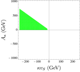
For the first solution ($s_{+}$) these result in figure 1. The top (bottom) panel corresponds to the case of stable (metastable) minimum. From left to right, the plots illustrate the effects of requiring successively non-tachyonic singlet scalars, as mentioned above. Clearly, with $s_{+}$, stable minima occur only for $A_{\kappa}\geq 0$. As can be clear from equation 33, demanding a non-tachyonic $CP$-odd singlet scalar (i.e., $\mathcal{M}_{P,22}^{2}\geq 0$) further restricts this region to $\kappa v_{{}_{S}}<0$ in the second column. Requiring on top of that the $CP$-even singlet scalar to be non-tachyonic (i.e., $\mathcal{M}_{S,33}^{2}\geq 0$) retains only the lower green wedge in the rightmost plot of the first row.

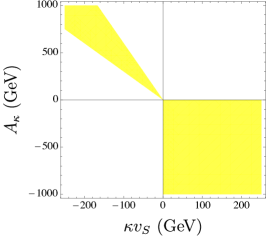
It may be noted that for the plots in the first column, the shaded regions in green (first row) and yellow (second row) are complementary in nature. This is trivially expected since if one of the minima is the global one, the other one has to be local in nature. The complementarity is carried over to the second column for which the singlet $CP$-odd scalar is required to be non-tachyonic. However, this is no more the case when one demands, in the third column, the same for the singlet $CP$-even scalar. There, a narrow (yellow) slice indicating metastability for $\kappa v_{{}_{S}}<0$ and $A_{\kappa}>0$ survives along with the yellow wedge that directly complements a similar green region but with opposite signs on $\kappa v_{{}_{S}}$ and $A_{\kappa}$, for the first solution.

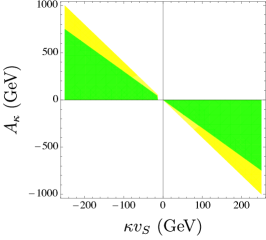
Furthermore, it can be found from table 1 that perfectly viable (corresponding) regions with flipped signs on the coordinates show up with the other non-vanishing solution $s_{-}$. This can be understood if we take note, in conjunction, of equation 28, in particular, its last term. Such flips may have important phenomenological implications. Note that existing works Ellwanger:1996gw ; Ellwanger:1999bv ; Djouadi:2008uj discuss one or the other of these solutions. We instead include both solutions in our present analysis. Figure 2 shows the consolidated situation thereof. Global minima with non-tachyonic states are possible over the green regions. Regions of metastability are in yellow. The latter also spread below whole of the green parts. As a check, it may be noted that the gradients of the edges of various wedge-shaped regions appearing in all these plots perfectly derive from the respective conditions collected in table 1. It may be noted here that not all of the conditions indicated in table 1 would hold in generic situations where the doublet Higgs fields also acquire non-vanishing values.

Figure 1: Allowed regions in the $\kappa v_{{}_{S}}-A_{\kappa}$ plane (left column) with the solution $s_{+}$ compatible with stable (top panel, in green) and metastable (bottom panel, in yellow) DSB minimum. Plots in the second and the third columns demonstrate the effects of requiring successively non-tachyonic singlet scalars (see text for details).

Figure 2: Consolidated allowed regions in the $\kappa v_{{}_{S}}-A_{\kappa}$ plane including both solutions $s_{+}$ and $s_{-}$ and on imposing the requirement of non-tachyonic scalars.

3.1.2   Non-vanishing $H_{d}^{0}$ and $H_{u}^{0}$ and radiatively corrected potential

This is perhaps the point where we might rightly like to pause and understand the role of two unavoidable ‘complications’ that are going to be present beyond the simplistic analysis presented above. These are the presence of non-vanishing $H_{d}^{0}$ and $H_{u}^{0}$ and the inclusion of radiative correction (at the 1-loop level only, though) to the potential. As pointed out earlier, inclusion of additional directions in field space makes the analysis rather tedious and extracting useful information thereof becomes challenging.

At the tree level itself, the general scenario with three non-vanishing neutral Higgs fields differs from the case with only one of them acquiring non-zero value. This is since the former may receive non-negligible contribution from terms trilinear and quartic in fields (as can be seen in the expression for the potential in equation 6) even in the vicinity of the DSB vacuum given that ‘$S$’ could turn out to be large ($\mathcal{O}(10\,\mathrm{TeV})$) there.

Away from the DSB vacuum, with increasing magnitude of $H_{d}^{0},H_{u}^{0}$, the effect may alter the potential profile giving rise to deeper minima. This would then have a non-trivial bearing on the stability of the DSB vacuum. Note that some of these terms further contain ‘$\lambda$’ multiplied to them. Hence in scenarios with small $\lambda$, the effect can only be moderate. For larger $\lambda$, the impact could be drastic. The inclusion of radiative correction further complicates the issue. As a result, the setup develops an intricate dependence on the NMSSM parameters.

Nonetheless, interestingly enough, all these complications can still be handled semi-analytically, to a very good extent. Such an approach would help understand the behaviour of the Higgs potential in arbitrary directions in the field space, away from the DSB. We undertake such an analysis via Mathematica which is similar to the one described in the previous subsection, this time the starting point being the full tree-level Higgs potential of equation 6.

For a given set of input parameters, at each stage, we use the appropriate set of tadpole equations to find the values for $m_{{}_{H_{d}}}^{2}$, $m_{{}_{H_{u}}}^{2}$ and $m_{{}_{S}}^{2}$ by requiring a DSB minimum at $\langle S\rangle=v_{{}_{S}}={\mu_{\mathrm{eff}}/\lambda}$. All parameters appearing in the potential are thus ‘locked’ and one can now find the potential profile as a function of the three neutral scalar fields. This reveals if there exists a minimum deeper than the DSB one (the panic situation). Radiative correction to the tree-level potential at the 1-loop level (see equation 11) is estimated using the field-dependent mass-squared matrices that are extracted from the tree-level potential. Thus, corrected $m_{{}_{H_{d}}}^{2}$, $m_{{}_{H_{u}}}^{2}$ and $m_{{}_{S}}^{2}$, obtained further as solutions to the tadpoles of the 1-loop effective potential, bear implicit field-dependence.

It is important to realize at this point that a general study of false vacua involving all three neutral scalar fields of the NMSSM gets to be rather involved and tedious. Along with the fields, a multitude of input parameters also enter the picture and hence add to the complication. It is thus necessary to have an optimal approach in exploring the scenario. This would help understand the underlying physics better and extract systematically information that are phenomenologically relevant and/or interesting. To this end, we divide the NMSSM parameter space into two broad categories:

• a scenario with small $\lambda(\lesssim 0.1)$, thus requiring large radiative corrections to have the mass of the SM-like Higgs boson in the right ballpark. In this sense, the situation is akin to the MSSM and hence the scenario is dubbed here as ‘MSSM-like’. A large radiative contribution is ensured primarily by setting the soft parameters pertaining to the third generation at $\mathcal{O}$(TeV);

• a scenario with somewhat large $\lambda\,(\lesssim 0.7)$. As is well known, such large values of $\lambda$ could push the mass of the SM-like Higgs boson substantially up at the tree level itself thus diminishing the need of radiative contributions to the same that are so indispensable in the MSSM. Naturally, the resulting scenario is dubbed ‘NMSSM-like’ in the present work.

A further classification is done based on a phenomenologically interesting possibility that the LSP (lightest supersymmetric particle)-neutralino in the NMSSM could essentially be a mixture of only the singlino and the higgsinos. The corresponding sub-classes are indicated in this work as scenarios which are ‘singlino-like’ and ‘higgsino-like’ requiring at least 75% admixture of singlino and higgsinos in the LSP, in the respective cases. For a general but concise understanding of the involved neutralino and the Higgs states, in particular reference to their singlet sectors, we refer the reader to section 2.2.

Parameters	Quantity	Mathematica v10	SPheno v3.3.8
	$V^{{}^{\mathrm{neutral}}}_{\mathrm{Higgs|1-loop}}$ @ DSB (GeV4)	$-6.18*10^{12}$	$-6.08*10^{12}$
Set A
	$\left\{m_{{}_{H_{u}}}^{2}/\,m_{{}_{H_{d}}}^{2}/\,m_{{}_{S}}^{2}\right\}_{\mathrm{1-loop}}$ (GeV2)	$1.79*10^{5}/8.96*10^{6}/4.99*10^{3}$	$1.78*10^{5}/8.96*10^{6}/4.99*10^{3}$
	$V^{{}^{\mathrm{neutral}}}_{\mathrm{Higgs|1-loop}}$ @ DSB (GeV4)	$-6.76*10^{12}$	$-6.53*10^{12}$
Set B
	$\left\{m_{{}_{H_{u}}}^{2}/\,m_{{}_{H_{d}}}^{2}/\,m_{{}_{S}}^{2}\right\}_{\mathrm{1-loop}}$ (GeV2)	$2.45*10^{5}/1.29*10^{7}/1.86*10^{4}$	$2.42*10^{5}/1.29*10^{7}/1.86*10^{4}$
	$V^{{}^{\mathrm{neutral}}}_{\mathrm{Higgs|1-loop}}$ @ DSB (GeV4)	$1.88*10^{12}$	$1.85*10^{12}$
Set C
	$\left\{m_{{}_{H_{u}}}^{2}/\,m_{{}_{H_{d}}}^{2}/\,m_{{}_{S}}^{2}\right\}_{\mathrm{1-loop}}$ (GeV2)	$8.96*10^{4}/4.46*10^{5}/2.22*10^{4}$	$9.68*10^{4}/4.51*10^{5}/2.24*10^{4}$
	$V^{{}^{\mathrm{neutral}}}_{\mathrm{Higgs|1-loop}}$ @ DSB (GeV4)	$1.88*10^{12}$	$1.85*10^{12}$
Set D
	$\left\{m_{{}_{H_{u}}}^{2}/\,m_{{}_{H_{d}}}^{2}/\,m_{{}_{S}}^{2}\right\}_{\mathrm{1-loop}}$ (GeV2)	$-2.82*10^{4}/2.50*10^{5}/8.16*10^{4}$	$-2.35*10^{4}/2.56*10^{5}/8.17*10^{4}$

Table 2: Numerical comparison of the values of the 1-loop radiatively-corrected neutral scalar potential and the resulting squared soft masses as obtained from a Mathematica-based analysis and Vevacious for the following sets of inputs parameters:
          Set A:    $\lambda=0.15,\,\kappa=0.01,\,A_{\lambda}=3000\,\mathrm{GeV},\,A_{\kappa}=0,\,\mu_{\mathrm{eff}}=100\,\mathrm{GeV},\,\tan\beta=30$;
          Set B:    $\lambda=0.06,\,\kappa=0.05,\,A_{\lambda}=5000\,\mathrm{GeV},\,A_{\kappa}=-500\,\mathrm{GeV},\,\mu_{\mathrm{eff}}=250\,\mathrm{GeV},\,\tan\beta=10$;
          Set C:    $\lambda=0.675,\,\kappa=0.1,\,A_{\lambda}=800\,\mathrm{GeV},\,A_{\kappa}=-450\,\mathrm{GeV},\,\mu_{\mathrm{eff}}=400\,\mathrm{GeV},\,\tan\beta=1.65$;
          Set D:    $\lambda=0.75,\,\kappa=0.5,\,A_{\lambda}=200\,\mathrm{GeV},\,A_{\kappa}=-850\,\mathrm{GeV},\,\mu_{\mathrm{eff}}=400\,\mathrm{GeV},\,\tan\beta=2$.
The soft mass-squared parameters and the soft trilinear parameters for the third generation squark sector are fixed at the following values: for sets ‘A’ and ‘B’, $m_{\widetilde{Q}_{3}}=m_{\widetilde{U}_{3}}=m_{\widetilde{D}_{3}}=3$ TeV and $A_{t}=3$ TeV; for sets ‘C’ and ‘D’, $m_{\widetilde{Q}_{3}}=m_{\widetilde{U}_{3}}=750$ GeV, $m_{\widetilde{D}_{3}}=3$ TeV and $A_{t}=0$, where $m_{\widetilde{Q}_{3}}$, $m_{\widetilde{D}_{3}}$ and $m_{\widetilde{U}_{3}}$ stand for the soft masses for the doublet, the up-type singlet and the down-type singlet squarks and $A_{t}$ is the trilinear coefficient for the stop sector. All other trilinear parameters are set to zero while the other scalar masses are taken to be heavy enough. Soft masses in the gaugino sector are all set to 2 TeV. The cutoff/renormalization scale $Q$ (equation 18) is chosen to be $Q=\sqrt{m_{\widetilde{Q}_{3}}m_{\widetilde{U}_{3}}}$.

In table 2 we compare some relevant quantities obtained from our Mathematica-based analysis with the ones from SPheno (which Vevacious uses). A few representative sets of parameters are chosen (indicated in the table-caption) which we would put to context later and use them further. The level of overall agreement is rather compelling (within 5%; except for the value of $m_{{}_{H_{u}}}^{2}$ at the 1-loop level in Case C where the deviation is about 8%). This would serve as a robust basis when we try to make sense of results obtained from Vevacious (modulo the thermal effects) in terms of our semi-analytical approach to the problem.

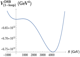
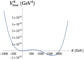
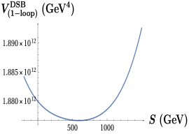
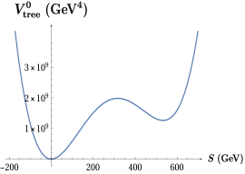
In figures 3 and 4 we illustrate the aforesaid effects via a set of potential profiles for scenarios presented in table 2. For each figure the top (bottom) row corresponds to the case with a singlino-like (higgsino-like) LSP In each row the leftmost plot is with $H_{d}^{0}=H_{u}^{0}=0$ and only ‘$S$’ is non-vanishing (equation 28). The middle one is with non-vanishing $H_{d}^{0}$ and $H_{u}^{0}$ (equation 6) fixed at their values at the DSB vacuum Note that this choice confines us to a direction normal to the $H_{d}^{0}$-$H_{u}^{0}$ plane, passing through it at a point with polar coordinates ($v=\sqrt{v_{d}^{2}+v_{u}^{2}},\,\beta=\tan^{-1}{v_{u}\over v_{d}}$) and extended in the $\pm S$ direction. Clearly, it should then be noted that these profiles do not reveal the actual ‘terrain’ of the potential in higher field dimensions and deeper minima could appear away from the chosen direction. Finally, plots in the rightmost column demonstrate the effect of adding radiative correction to the potential.

Figure 3: Profiles of the neutral scalar potential as a function of the field ‘$S$’ in the MSSM-like scenario. The top (bottom) panel stands for the case with a singlino- (higgsino)-like LSP. Left panel shows the tree-level profiles when ‘$S$’ is the only scalar field present. Plots in the middle panel illustrate the situation with non-vanishing $H_{d}^{0}$ and $H_{u}^{0}$ while their values are fixed at the respective vevs they assume at the DSB minimum. Further, profiles in the rightmost panel result from the consideration of 1-loop radiatively-corrected potential. $V^{0}$ is evaluated with $H_{u}^{0}=H_{d}^{0}=0$ whereas $V^{\mathrm{DSB}}$ is computed by fixing the Higgs fields at their DSB values.

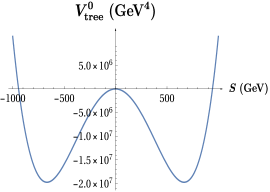
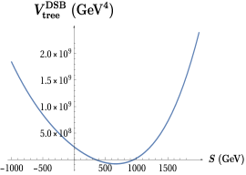
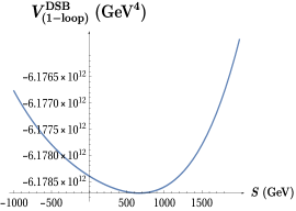
The leftmost plot in the first row of figure 3 has a symmetric profile under $S\rightarrow-S$ with a degenerate pair of minima. This is understood in terms of vanishing $A_{\kappa}$ that we set for this row which makes the only term with odd (cubic) power on ‘$S$’ (for vanishing $H_{d}^{0}$ and $H_{u}^{0}$) in equations 6 also vanishing. As can be seen from the middle plot, switching on finite values of $H_{d}^{0}$ and $H_{u}^{0}$ lifts this degeneracy. Thus, the only minimum appears for a positive value of ‘$S$’ ($\sim 670$ GeV). This is indeed where the DSB vacuum should appear given our choices of $\mu_{\mathrm{eff}}$ (=100 GeV) and $\lambda$ (=0.15) for the case in hand. The rightmost plot in this panel shows that the inclusion of radiative correction roughly preserves the shape of the profile. However, as expected, the amount of (negative) correction is appreciable. Plots in the second row of figure 3 reveal that there may be a situation when the profile may not get distorted at all, although, radiative correction does alter the scale of the potential. As discussed earlier, introducing non-vanishing $H_{d}^{0}$ and $H_{u}^{0}$ has hardly any effect on the potential in this case since $\lambda$ is set to a small value (=0.06).

Figure 4: Same as in figure 3 but for the NMSSM-like case.

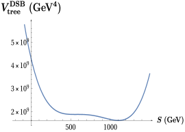
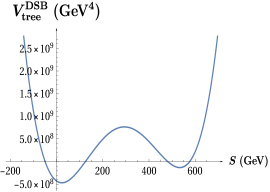
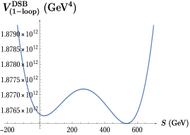
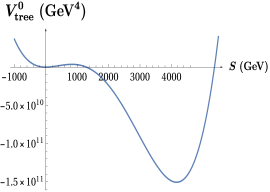
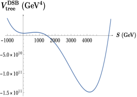
The plot in the left column of figure 4 refers to a situation where the would be DSB vacuum starts off as a local maximum of the tree-level potential (with $H_{d}^{0}=H_{u}^{0}=0$) at $S={\mu_{\mathrm{eff}}\over\lambda}\approx 590$ GeV. Finite $H_{d}^{0}$ and $H_{u}^{0}$ turn this, to be precise, into a point of inflection (middle plot) before radiative effects make this the DSB vacuum which is also the global minimum. On the other hand, the leftmost plot in the second row of figure 4 describes a situation where the DSB minimum is a local one. Finite $H_{d}^{0}$ and $H_{u}^{0}$ affect the profile to a moderate extent by decreasing the relative depths between the DSB and the global minimum (middle plot). Further, radiative correction turns the DSB minimum into the global minimum of this (single-field) potential.

Figure 5: Contour profiles of the 1-loop radiatively-corrected potential (containing all three neutral scalar fields) $S-H_{u}^{0}$ plane along the fixed $H_{d}^{0}$ directions that yield the deepest (global) minima in respective cases. Top (bottom) panel presents the MSSM-like (NMSSM-like) scenario. In each case, the plot on left (right) illustrates the situation with a singlino- (higgsino)-like LSP. Pallets below the plots shows the color codes indicating the magnitude of the effective potential. The bullet in each plot points to the actual location of the global minimum in the field space.

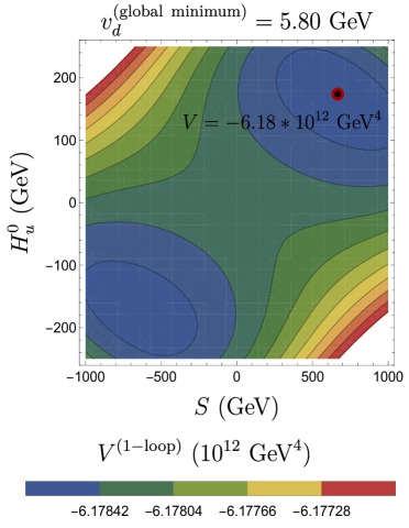
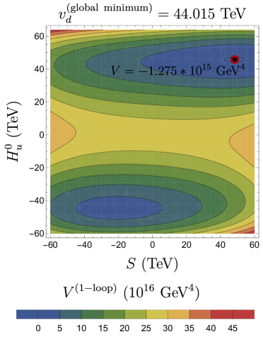
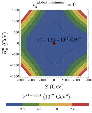
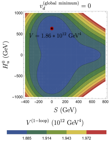
An important purpose of the present study is to have the idea about where exactly the extrema appear in the field-space. With this in mind, in figure 5 we present the ‘iso-potential’ (radiatively corrected) contours for the four sets of parameters used in figures 3 and 4. However, this time we move away from the fixed directions adopted there and choose the ones along which the global (deepest) minimum of the potential occur for each case. As can be seen, all these are either along or very close by to some flat directions. We indicate the location of the global minimum on the $S-H_{u}^{0}$ plane in each case and mention the magnitudes of the potential. These values can be compared straightaway to the ones associated with the corresponding DSB minima shown in the rightmost column of 3 and 4. Furthermore, plots in figure 5 also convey that regions in the field space with deeper potential are always surrounded from all sides by regions with higher values of the potential. This implies that in all these cases the potential is bounded from below as it should be in a realistic situation. However, presence of dangerous directions along which the potential is unbounded from below (UFB) are still possible Ellwanger:1999bv ; Abel:1998ie . This is in spite of having positive contributions to the potential from $v_{{}_{S}}$ which generally come in rescue.

3.2 False vacua along arbitrary field directions: a semi-analytical study

Given the discussion in section 3.1.2, it would now be easier to appreciate how involved a study of false vacua arising along arbitrary directions in the NMSSM field space could get. Such a study not only involves a larger volume of a multi-dimensional parameter space but also opens up to variations of all relevant NMSSM fields. Thus, a reasonable scan over the parameter space gets rather time-consuming even in a state-of-the-art (multi-processing) computing environment. Hence, in this section and in the rest of this work, we would adhere to the broad scenarios introduced in section 3.1.2. In order to deal with the emerging intricacies, we also generalize the scope of our Mathematica-based code in an appropriate manner.

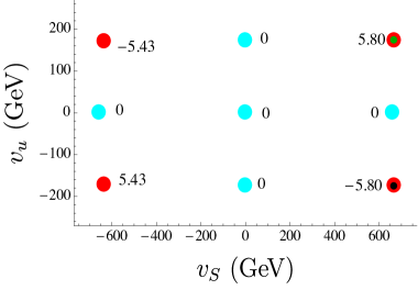
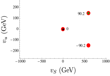
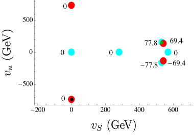
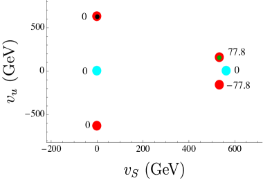
The complete picture pertaining to the locations of the extrema of the potential, in particular, those of the DSB minimum and the global minimum, is illustrated through figures 6 and 7 for the MSSM- and the NMSSM-like cases, respectively. The top (bottom) rows correspond to the cases with a singlino- (higgsino)-like LSP. The left (right) columns stand for the situations with the tree-level (1-loop effective) potential with non-vanishing $H_{d}^{0}$, $H_{u}^{0}$ and ‘$S$’. All three fields are allowed to vary simultaneously. Coordinates of the bullets point to the locations of these extrema in the $S-H_{u}^{0}$ plane. Values assumed by $H_{d}^{0}$ are indicated (in GeV) alongside the bullets. Following color convention is adopted to indicate the nature of the extrema: red for minima, black within red for the global minimum, green within red for the DSB minima and cyan for the saddle points. Thus, a bullet having red, green and black all appearing in it represents a DSB minimum which, at the same time, is the global minimum of the potential. The following general remarks/observations would be in place.

• Search for extrema of the 1-loop effective potential is performed in Mathematica with the tree-level extrema as the guess values.

• An exact symmetry under $H_{d}^{0},H_{u}^{0}\to-H_{d}^{0},-H_{u}^{0}$ is apparent at the tree level which is mostly holding with the 1-loop effective potential.

• There is no general correspondence among various extrema found for the tree-level and the corrected potential, except for the DSB extrema for which the nature may get altered, though. For example, the DSB extremum in the NMSSM-like scenario with a singlino-like LSP (top, left plot of figure 7) appears to be a saddle point with tree-level potential. This becomes a likely global minimum when the corrected potential is used.

It may also be noted that figure 6 (figure 7) connects to figure 3 (figure 4) via the locations of the DSB minima. On the other hand, the right plots of the former set of figures connect to the plots in the top (bottom) row of figure 5 via the coordinates of the global minima which are not necessarily the DSB minima. These connections are explicitly indicated on individual plots of figures 6 and 7. In particular, it is noted that in the MSSM-like scenario with a higgsino-like LSP (bottom, right plot of figure 6 and top, right plot in figure 5) the global minimum occurs for large values of ‘$S$’ with $H_{d}^{0}\approx H_{u}^{0}$, i.e., approximately along the $D$-flat direction. It would be interesting to see if our subsequent analysis using Vevacious corroborates this fact along with other findings from our studies so far.

Thus, the left plots in figure 6 (figure 7) are to be compared with the middle plots of figure 3 (figure 4). Similarly, the right plots in figure 6 (figure 7) are to be compared with the rightmost plots of figure 3 (figure 4). The latter set of four plots (having the radiative effects included) are also to be compared with the corresponding ones from a similar set in figure 5.

Figure 6: Locations of all the extrema (in the $S$-$H_{u}^{0}$-$H_{d}^{0}$ space) found in the MSSM-like scenario with a singlino-like (top panel) and higgsino-like (bottom panel) LSP and with the tree-level (left panel) and the 1-loop corrected (right panel) potential. Red bullets represent (local) minima, black-centered red bullets indicate global minimum, green-centered red bullets stand for DSB minimum and bullets in cyan point to saddle points of the potential. Numbers alongside the bullets indicate the corresponding magnitudes of $H_{d}^{0}$ (in GeV).

Figure 7: Same as in figure 6 but for the NMSSM-like scenario.

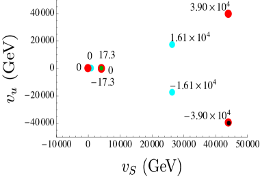
The MSSM-like scenario is broadly realized by choosing small values of $\lambda$ ($\lesssim 0.1$). However, in view of the possibility discussed in footnote 7, we allow for a little wider range of $\lambda$ spanning over an order of magnitude that also includes somewhat large values of $\lambda$. Thus, scan is done over the following ranges of the relevant set of parameters:

$$10^{-4}<\lambda<0.75,\quad 10^{-3}<|\kappa|<0.75,\quad|A_{\lambda}|<7.5\,\mathrm{TeV},\quad|A_{\kappa}|<7.5\,\mathrm{TeV},$$

$$\quad|\mu_{\mathrm{eff}}|<500\,\mathrm{GeV},\quad 1<\tan\beta<50\quad.$$ (34)

Note that for a smaller $\lambda$ ($\sim 0.01$), to obtain $\mu_{\mathrm{eff}}$ in the phenomenologically right ballpark ($|\mu_{\mathrm{eff}}|\sim\cal{O}$(100 GeV)), $v_{{}_{S}}={\mu_{\mathrm{eff}}\over\lambda}$ could turn out to be rather large ($\gtrsim\cal{O}$(10 TeV)). Since for the DSB minimum the vevs $v_{d}$ and $v_{u}$ cannot be too large ($\lesssim\cal{O}$(100 GeV)), the potential in the vicinity of the same can be approximated as a function of only one scalar field, ‘$S$’. Thus, the previous analysis in section 3.1.1 based on equation 28 could be largely applicable for the MSSM-like scenario.

On the other hand, we confine the NMSSM-like scenario in a region with relatively larger values of $\lambda$, as it should be by its definition. Thus, we set the following ranges for scanning the parameter space:

$$0.5<\lambda<0.75,\quad 10^{-3}<|\kappa|<0.75,\quad|A_{\lambda}|<2.5\,\mathrm{TeV},\quad|A_{\kappa}|<2.5\,\mathrm{TeV}$$

$$\quad|\mu_{\mathrm{eff}}|<500\,\mathrm{GeV},\quad 1<\tan\beta<5\quad.$$ (35)

For the set of various fixed input parameters used in this part of the analysis, the reader is referred to the caption of table 2. Note that ranges of the NMSSM parameters that are varied in these two broad scenarios are rather different. These are primarily so to ensure acceptable (non-tachyonic) values for various Higgs masses.

Figure 8: Scatter plot from the Mathematica-based analysis showing allowed regions in the $\kappa v_{{}_{S}}-A_{\kappa}$ plane compatible with stability (in blue) and metastability (in golden yellow) of the DSB vacuum and also with non-tachyonic neutral scalar states. See text for the ranges of various input parameters used in the scan. The upper (lower) panel stands for the MSSM-like (NMSSM-like) scenario. The left (right) column presents the case with a singlino-like (higgsino-like) LSP.

We now perform random scans of the NMSSM-parameter space with the Mathematica-based analysis routine we develop. Scans are done for the two scenarios discussed above and over the respective sets of ranges for various NMSSM inputs as indicated in equations 34 and 35. While scanning, we confine ourselves to the tree-level potential since inclusion of radiative correction makes the scan prohibitively slow.

In figure 8 we present the results of the scan in the $\kappa v_{{}_{S}}-A_{\kappa}$ plane in the form of scatter plots. The upper (lower) panel illustrates the situation in the MSSM-like (NMSSM-like) case while the left (right) column stands for the situation where the LSP is singlino-like (higgsino-like). Over the regions in blue the DSB minimum emerges as the global minimum and hence stable. The golden-yellow region stands for a situation where the DSB minimum is the local minimum of the potential and hence metastable. Among these plots, the upper, left one representing the MSSM-like case and having a singlino-like LSP, can be taken a particular note of. This approximately corresponds to the setup with the single field (‘$S$’) potential elaborated in section 3.1.1 and is illustrated in figure 2. It is rather convincing to find how decently the regions obtained through a purely analytical treatment (see figure 2) are now reproduced in this scan which is semi-analytic in nature. In general, figure 8 would serve as a useful reference for a subsequent analysis taken up in section 3.3 using Vevacious.

3.3 False vacua along arbitrary field directions: a Vevacious-based study

In this subsection we discuss issues pertaining to the stability of the DSB vacuum in the $Z_{3}$-symmetric NMSSM by subjecting its parameter space to a thorough analysis via Vevacious Camargo-Molina:2013qva , a state-of-the-art package dedicated for the purpose. Its working principle has been briefly outlined in section 2.3.

An analysis of stability of the NMSSM vacuum using Vevacious would take us beyond the Mathematica-based analysis we presented in section 3.2 in two important aspects. As pointed out in section 2.3, Vevacious includes both quantum and thermal corrections to the potential (which is proven to be crucial for the purpose) and computes the tunneling time of the DSB vacuum to a deeper (panic) minimum. Furthermore, such a study can be seamlessly interfaced to other external packages for an in-flight analysis of the viability of a given point in the parameter space against other experimental constraints. These make the analysis all the more realistic. In the following, we outline the broad categories into which Vevacious classifies the fate of the DSB vacuum. These are later exploited in our presentation.

• Stable: when the DSB vacuum is the global minimum of the potential;

• Metastable but long-lived: when there is a minimum deeper (global minimum) than the DSB vacuum (local minimum) but the decay time of the DSB vacuum to this is large enough in reference to the age of the Universe (not only at zero temperature but also when thermal effects are included) so that it could safely be considered viable;

• Metastable but short-lived at zero temperature: when the decay time of the DSB vacuum to such a deeper minimum is short enough under a rapid quantum tunneling at zero temperature thus making the former unstable and thus, inviable;

• Metastable but short-lived only at finite temperatures: when the instability of the DSB vacuum is triggered only at finite temperatures.

In table 3 we collect the corresponding number codes used by Vevacious to flag each of these situations along with the color codes we use for these in some of the subsequent scatter plots.

Stability/Longevity of		Viability of	Color-code
the DSB vacuum	Vevacious code	the DSB vacuum
Stable	1	Viable	$\bullet$ Green
Metastable but long-lived	0	Viable	$\bullet$ Blue
Metastable but short-lived	-1	Not Viable	$\bullet$ Black
(tunneling at zero temperature)
Metastable but short-lived	-2	Not Viable	$\bullet$ Red
(tunneling at finite temperature)

Table 3: Vevacious numeric codes flagging specific status and viability of the DSB vacuum and the corresponding color codes used subsequently in this work.

Scans are done over the same set of parameters, over the same ranges (see expressions 34 and 35 and the caption of table 2) and referring to the same set of scenarios as have been adopted for the Mathematica-based scan presented in section 3.2. SLHA Allanach:2008qq files containing the spectrum and other important information obtained from SARAH v4.5.8-generated Staub:2013tta ; Staub:2015kfa SPheno v3.3.8 Porod:2003um ; Porod:2011nf are fed into Vevacious.

We also keep track of the following issues which are of phenomenological importance. One of the $CP$-even Higgs states is required to have a mass within the range $122$-$128$ GeV and should behave like the SM-like Higgs boson. This is ensured by subjecting the analysis to treatments by HiggsBounds v4.3.1 Bechtle:2013wla and HiggsSignals v1.4.0 Bechtle:2013xfa in parallel. Furthermore, we subject the analysis to important current bounds from the flavor sector in the form of $B\to X_{s}\gamma$, allowing for the range $2.77\times 10^{-4}\leq\mathrm{BR}[B\to X_{s}\gamma]\leq 4.09\times 10^{-4}$ at $3\sigma$ level Amhis:2012bh via SPheno, from the dark matter sector (in the form of a $5\sigma$ upper bound on its relic density which is taken to be $\Omega_{\mathrm{CDM}}h^{2}<0.127$ Ade:2015xua ) via micrOMEGAs v4.2.5 Belanger:2014vza and to the lower bound of the chargino mass of 103 GeV lepsusy which is close to the kinematic threshold of the LEP experiments. However, unless specifically mentioned, the figures we present subsequently are obtained without imposing these constraints (except for respecting the bound on the chargino mass and requiring a Higgs boson with a mass in the range mentioned above). This is to ensure that the basic features and constraints obtained from the bare analysis of the possible vacua first get clarified.

3.3.1   Scanning of the MSSM-like scenario with Vevacious

To ensure an optimally large radiative correction to the mass of the SM-like Higgs boson that defines the MSSM-like scenario in this work, we set the soft masses of all the sfermions at a somewhat large value of 3 TeV. The soft trilinear coupling $A_{t}$ in the top squark sector is also fixed at 3 TeV while the same for the bottom ($A_{b}$) and the tau ($A_{\tau}$) sectors are set to zero.

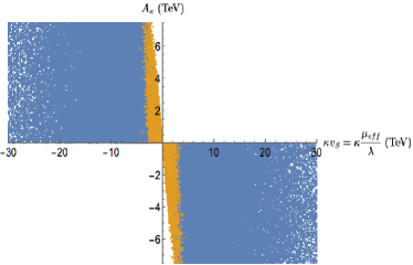
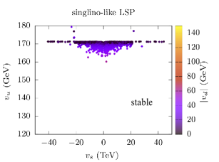
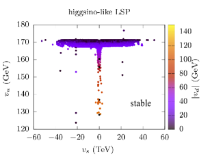
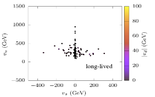
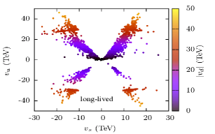
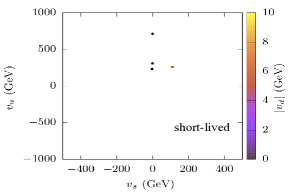
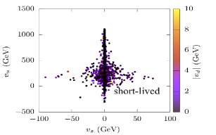
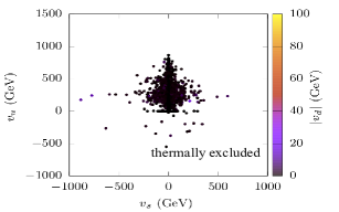
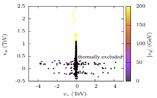
In figure 9 we illustrate the nature of stability of the DSB vacuum in terms of the vevs acquired by the fields ‘$S$’ ($v_{{}_{S}}$) and $H_{u}^{0}$ ($v_{u}$) at the DSB vacuum and other deeper minima. The absolute value of the vev of the third neutral scalar field, $H_{d}^{0}$ ($|v_{d}|$) is indicated via adjacent color palettes. Columns stand for scenarios with a singlino-like (left) and a higgsino-like (right) LSP. Rows present possible fates of the DSB vacuum which are summarized in section 3.3. From top to bottom, in that order, the plots show the field values consistent with (i) the DSB vacua which are stable (top row), (ii) the deeper minima with which the DSB minima become metastable but long-lived (second row), (iii) the same which make the DSB vacua metastable and short-lived under zero-temperature quantum tunneling (third row) and (iv) the same that render the DSB vacua metastable and short-lived only with thermal effects factored in (last row). Thus, parameter points in the first two rows yield viable DSB vacua while, in the latter two, they do not. The following set of observations are in order.

Figure 9: Regions in the $v_{{}_{S}}$-$v_{u}$-$v_{d}$ space in the MSSM-like scenario obtained from Vevacious scan that lead to (i) a viable DSB vacuum which is the global minimum of the potential (top row), (ii) a global minimum that is deeper than the (metastable) DSB vacuum but the latter being still long-lived enough and hence viable (second row), (iii) the same but the DSB vacuum being short-lived under zero-temperature quantum tunneling and hence not viable (third row) and (iv) the same but when the DSB vacuum is short-lived and thus, not viable, only if thermal effects to the potential are included (bottom row). The left (right) panel stand for the cases with a singlino- (higgsino)-like LSP. Colors represent values taken by $|v_{d}|$ as shown in the accompanying pallets. The ranges of various parameters used in the scan are as given in expression 34.

• It can be clearly recognized that the sets of three vev-values that emerge for each scattered point in the plots in the first row of figure 9 are in compliance with a DSB vacuum and are consistent with the values of the supplied NMSSM input parameters, in particular, those for $\mu_{\mathrm{eff}}$ and $\lambda$.

• For the rest three rows the vevs refer to minima deeper than the DSB vacuum thus making the latter metastable. These reveal that deeper minima might appear for rather high values (reaching up to tens of TeV) for all three fields. These are in addition to deeper minima that occur along some flat directions in the field space which are already known to be the ‘dangerous’ for the stability of the DSB vacuum. In particular, the plots indicate that the direction $H_{d}^{0}=S=0$ is such a flat direction.

• Furthermore, a closer look at the right plot in the second row (long-lived DSB vacuum in the higgsino-dominated LSP case) reveals that deeper minima causing the DSB vacua to be metastable but long-lived occur along the diagonals. These correspond to directions which are both (approximately; at the 1-loop level) $D$-flat ($H_{d}^{0}\approx H_{u}^{0}$) and $F_{S}$-flat ($S^{2}\approx\frac{\lambda}{\kappa}H_{d}^{0}H_{u}^{0}$; see section 3.1) in the field space.

• It is important to note from the plot on the left in the third row (singlino-like LSP case) that tunneling at zero temperature does note pose a threat to the stability of the DSB vacuum. Plots from the fourth row clearly reveal that the thermal effect indeed plays an important role in determining the fate of metastable DSB vacua. Had it not been for the thermal contributions, these regions would have given rise to a deeper minimum which could still ensure long-lived DSB vacua. Some of these appear distinctively for somewhat large (compared to the values it may assume at the DSB, i.e., $\sim 125-175$ GeV) positive values of $H_{u}^{0}$ in the MSSM-like case and along the flat direction $S=H_{d}^{0}=0$ with magnitudes of $H_{u}^{0}$ comparable to its DSB value.

Figure 10: Regions in the $A_{\lambda}-A_{\kappa}$ plane showing the fate of the DSB vacuum for the MSSM-like scenario with a singlino-like LSP (left) and with a higgsino-like LSP (right). Refer to table 3 for the color-code used.

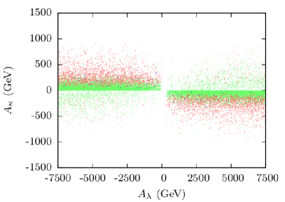
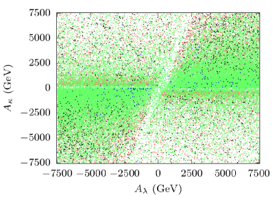
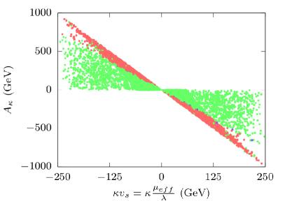
As may be expected from earlier studies in the MSSM, the trilinear terms in the NMSSM sector as well, are likely to play some important role in determining the stability of the DSB vacuum. In figure 10 we illustrate the stability pattern of the DSB vacua in the $A_{\lambda}-A_{\kappa}$ plane in the MSSM-like scenario and for the cases where the LSP is singlino-like (left plot) and higgsino-like (right plot). An analysis of a similar effect but applied in the context of dark matter phenomenology has been carried out earlier in reference Cerdeno:2004xw . The features of these plots, which we will discuss shortly, would be easier to understand once we consider the following issues.

The singlet $CP$-even and $CP$-odd scalar masses in the MSSM-like scenario, for large $v_{{}_{S}}$, can be written down as (from equations 15 and 19)

$$\mathcal{M}_{S,33}^{2} \approx \kappa v_{{}_{S}}(A_{\kappa}+4\kappa v_{{}_{S}})$$ (36a)

$$\mathcal{M}_{P,11}^{2} = {{2\mu_{\mathrm{eff}}\,(A_{\lambda}+\kappa v_{{}_{S}})}\over{\sin 2\beta}}$$ (36b)

$$\mathcal{M}_{P,22}^{2} \approx -3\kappa A_{\kappa}v_{{}_{S}}\quad.$$ (36c)

This is reminiscent of the discussion we had in the context of the study of single-field ($S$) potential in section 3.1.1. Requiring $\mathcal{M}_{P,22}^{2}>0$ yields $\kappa v_{{}_{S}}A_{\kappa}<0$. When this is combined with the demand of $\mathcal{M}_{S,33}^{2}>0$, one finds $|A_{\kappa}|<4|\kappa v_{{}_{S}}|$, i.e., the magnitude of $A_{\kappa}$ is bounded from above. This is clearly seen in the case with a singlino-like LSP (left plot) for which $|\kappa v_{{}_{S}}|$ cannot exceed $\frac{|\mu_{\mathrm{eff}}|}{2}$. Given that we scan over the range $|\mu_{\mathrm{eff}}|<500$ GeV, $|A_{\kappa}|$ cannot exceed 1 TeV. On the other hand, in the case with a higgsino-like LSP, $|\kappa v_{{}_{S}}|$ can be legitimately large compared to $\frac{|\mu_{\mathrm{eff}}|}{2}$ and thus $A_{\kappa}\sim\mathcal{O}(\mathrm{TeV})$ are also allowed. As may be apparent (and we will see soon) from the set of expressions in equation 36, demanding non-tachyonic scalar states might eventually lead to only a few discrete possibilities of relative signs and magnitudes among various NMSSM parameters.

Figure 11: Regions in the $\kappa v_{{}_{S}}-A_{\kappa}$ indicating the fate of the DSB vacuum in the MSSM-like scenarios with a singlino-like (left) and a higgsino-like (right) LSP. Color-code employed is as summarized in table 3.

In the left plot (the case with a singlino-like LSP) of figure 10 the first (second) and the third (fourth) quadrants with $A_{\lambda}A_{\kappa}>0\;(<0)$ correspond to $\kappa<0\;(>0)$. This is because of the following reason. Note that for the singlino-like case the product $\kappa v_{{}_{S}}$ is small and thus can be neglected. Demanding the $CP$-odd doublet scalar boson to be non-tachyonic, it follows from equation 36b that $\mu_{\mathrm{eff}}$ (i.e., $v_{{}_{S}}$) and $A_{\lambda}$ are of the same sign. Given that (see above) $A_{\kappa}$ and $\kappa v_{{}_{S}}$ are of opposite signs, a positive ‘$\kappa$’ requires $A_{\kappa}$ and $A_{\lambda}$ to be of opposite sign. The reverse is true for ‘$\kappa$’ being negative. A similar analysis mostly holds in the case with a higgsino-like LSP (right plot) with the exception that one may not be able to neglect the magnitude of $\kappa v_{{}_{S}}$ here. In this case its cancellation against $A_{\lambda}$ on the right-hand side of equation 36b is a possibility which could lead to a tachyonic doublet $CP$-odd scalar. This possibility shows up in a tilted edge (in contrast to a vertical one in the left plot) that separates the region with $\mu_{\mathrm{eff}}>0$ on the right side of the plot from that with $\mu_{\mathrm{eff}}<0$ on the left. In fact, we are able to predict correctly the magnitude of the tilt by using the set of above equations. Apart from that, we observe that DSB vacua with diverse stability properties could appear over the entire $A_{\lambda}$-$A_{\kappa}$ plane as shown in this plot.

Here we recall (see section 3.2) that the free parameter $A_{\kappa}$ plays a subtle role in the fate of the DSB vacuum in the MSSM-like scenario for which $v_{{}_{S}}>>v_{d},v_{u}$. In figure 11 we illustrate this through a Vevacious-based analysis. Color-code used is already introduced in table 3. We compare these plots with the plots in the top row of figure 8 (obtained from a Mathematica-based analysis) which also represent the MSSM-like scenario. For both sets plots on the left (right) correspond to the cases with singlino (higgsino-like) LSP. An impressive level of agreement does not escape notice.

Figure 12: Regions obtained from Vevacious scan in the $m_{{{}_{\chi}}_{1}^{0}}-m_{h_{1}}$ space indicating the fate of the DSB vacuum in the MSSM-like scenario with a singlino-like LSP (left panel) and a higgsino-like LSP (right panel). Plots in the top row incorporate all basic constraints along with those coming from HiggsBounds and HiggsSignals. Plots in the middle (bottom) row include, in addition, bounds from the flavor (dark matter) sector. Color-code employed is as summarized in table 3.

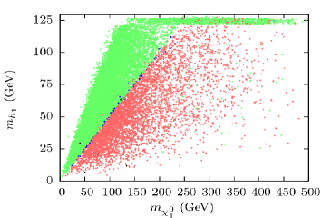
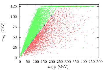
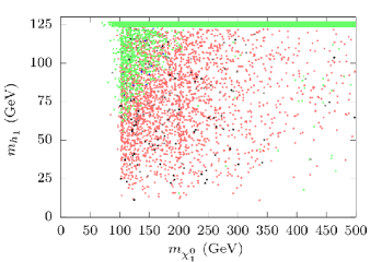
We now move on to discuss how the nature of the stability of the DSB vacuum is related to phenomenology. Issues that are of immediate interest in the NMSSM context pertain to the Higgs sector, especially the lighter Higgs bosons of the singlet kind and the lighter neutralinos which can have significant singlino admixture. Hence in figure 12 we illustrate how the stability of the DSB vacuum manifests itself in the $m_{{{}_{\chi}}_{1}^{0}}-m_{h_{1}}$ plane. As before, the left (right) column presents the singlino-like (higgsino-like) case. The first row uses the same set of data as for figures 9 and 11. Plots in the second row are obtained after subjecting these data sets to the scrutiny by HiggsBounds and HiggsSignals to ensure an overall conformity to the experimental findings on the SM-like Higgs boson. In addition, plots in this row are also in compliance with the constraint from the flavor sector as mentioned in section 3.3. Note, however, that in the scenario under discussion these do not have much bearing on the allowed region of parameter space. Plots in the third row depicts the situation further on the imposition of the upper bound on the DM relic density again as indicated in section 3.3.

It is clear that only the constraint pertaining to DM relic density and that also solely for the case with a singlino-like LSP have a noticeable bearing on the allowed region in the $m_{{{}_{\chi}}_{1}^{0}}-m_{h_{1}}$ plane. This is since a singlino-like LSP has in general a rather feeble interaction with other particles and thus its annihilation rates are suppressed giving rise to an unacceptable level of relic density. This is more so when $\lambda$ is small, which is generally the case with the MSSM-like scenario, thus suppressing its couplings with higgsino-like states in the spectrum. In contrast, a higgsino-like LSP can have a substantial couplings to other relevant states which may aid its rapid annihilation. In addition, for a higgsino-like LSP there is always a nearby light neutralino and chargino states which are also higgsino-like. These facilitate efficient coannihilation of the LSP.

Note that such an efficient coannihilation is also possible in the case with a singlino-like LSP once its mass comes closer to the higgsino-like states. In the left plot from the last row of figure 12 this is clearly the case when the LSP mass reaches 100 GeV. This is close to the minimum mass considered for the near-degenerate higgsino-like states with $|\mu_{\mathrm{eff}}|\geq 100$ GeV prompted by the lower bound (103 GeV) on the mass of the lighter chargino lepsusy as indicated in section 3.3. Furthermore, on the left of this plot there are also two green (vertical) strands separated by a gap. The left (right) strand occurs at an LSP-mass of $~{}45$ ($\sim 62-63$) GeV which clearly points to $s$-channel annihilation of a pair of LSPs via a resonant $Z$-boson (SM-like Higgs boson).

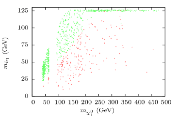
The message to take home from figure 12 is that the region of stability (in green) of the DSB vacuum is segregated from the region where it is metastable only for the cases with a singlino-like LSP. Crucially enough, the dominance of the color ‘red’ in this metastable regime indicates that it falls out of favor primarily on the inclusion of thermal effects. For cases with a higgsino-like LSP, the instability of the DSB vacuum is more pervasive. The region with a stable DSB vacuum for this case is mostly concentrated at lower masses for the LSP and for a singlet-like $CP$-even Higgs boson which is not much lighter than the SM-like Higgs boson. It may also be noted that for cases with a singlino-like LSP one mostly finds the region with $h_{1}$ as the SM-like Higgs boson to yield a stable DSB vacuum (the green horizontal bands about $m_{h_{1}}\sim 125$ GeV). However, for scenarios with a higgsino-like LSP this is not guaranteed. This is so since, in these cases, we notice that red horizontal bands (implying thermal instability) are hiding underneath the green ones about $m_{h_{1}}\sim 125$ GeV.

In general, we observe that the thermal effects become more significant with increasing $|A_{\kappa}|$ which turn the global (DSB) minimum to a local one by altering their depths. This may be quite expected given the discussion in the beginning of section 3.1. Had it not been for the thermal corrections, the red (unstable) region would have become viable being home to metastable but long-lived DSB vacua. This underscores the importance of a Vevacious-based analysis. A careful look at the plots in the left column for the first two rows also reveals thin streaks of regions (in blue) where the DSB vacua are indeed ‘long-lived’ and separate the green and the red regions. The role of thermal correction in this particular respect could be generically summarized as follows. We find that this introduces contributions cubic in the fields via a term $-{\pi\over 6}({m^{2}\over T^{2}})^{3/2}$ originating in the expansion of the (bosonic) quantity $J_{+}({m^{2}\over T^{2}})$ of equation 13. This might dilute the role of the tree-level term ${2\over 3}\kappa A_{\kappa}S^{3}$ and acts towards decreasing the barrier-height between the false (DSB) vacuum and the deeper (panic) vacuum thus facilitating the tunneling process.

It may be noted that since $\lambda$ and ‘$\kappa$’ are relatively small in the MSSM-like scenario, the singlet $CP$-even scalar can be naturally light. Thus, the SM-like Higgs boson (with a mass $\sim 125$ GeV) turns out to be predominantly a heavier $CP$-even Higgs boson over a significant part of the MSSM-like parameter space. Furthermore, the gradient of the left (outer) edge of the green patch for the plots in the left column can be understood by studying equation 22 that relates the masses of the $CP$-even singlet scalar and the singlino. In contrast, there appears a vertical edge at around 100 GeV for the LSP-mass in the plots in the right column. This is simply because these plots represent the case of a higgsino-like LSP which is roughly degenerate with the lighter chargino thus attracting a similar lower mass-bound ($\sim 103$ GeV) as for the latter.

An accompanying light $CP$-odd scalar would be phenomenologically (in particular, in the collider context) rather interesting. We find that in the MSSM-like scenario that we are discussing, a relatively light singlino-like LSP could appear along with light singlet-like $CP$-even and $CP$-odd scalars. All of them could have masses ($m_{{{}_{\chi}}_{1}^{0}}$, $m_{h_{1}}$ and $m_{a_{1}}$, respectively) in the order of a few tens of a GeV and can be consistent with all relevant experimental constraints and with the requirement of a stable DSB vacuum. This is possible since $\kappa v_{{}_{S}}$ is small for such a scenario and hence a small value of $|A_{\kappa}|$ suffices to yield a light $CP$-even scalar (see equation 36). This in turn keeps the mass of the singlet-like $CP$-odd scalar light. Interestingly, it is rather straightforward to find that the same set of equations predicts an anti-correlation between the compatible masses of these two states for cases with a higgsino-like LSP where $\kappa v_{{}_{S}}$ is required to be large. In this case it is noted that while $m_{a_{1}}\approx 50$ GeV can be compatible with $m_{h_{1}}\gtrsim 100$ GeV, $m_{h_{1}}\lesssim 50$ GeV could only be accompanied by $m_{a_{1}}\gtrsim 200$ GeV. These roughly summarize what could be the implications for the collider experiments of such a scenario with a stable vacuum.

3.3.2   Scanning of the NMSSM-like scenario with Vevacious

We take up a similar study using Vevacious on the nature of stability of the DSB vacuum in the NMSSM-like scenario and its phenomenological implications. In figure 13 we present the characteristic ranges of field-values. Plots are arranged in the same way as in figure 9. In this regard, some salient features of the NMSSM-like scenario, when compared to the MSSM-like case (figure 9) are as follows.

Figure 13: The same as in figure 9 but for the NMSSM-like scenario with ranges of various parameters used in the scan as given by expression 35.

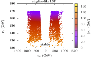
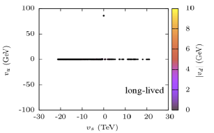
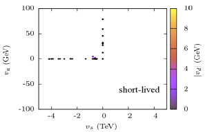
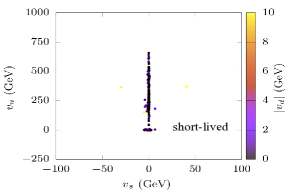
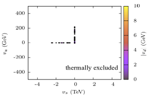
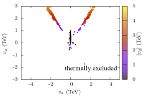
• Stable DSB vacua (first row) now appear more frequently over a little bigger ranges of $H_{d}^{0}$ and $H_{u}^{0}$ thanks to possible low values of $\tan\beta$. The relevant range for $v_{{}_{S}}$ at the stable DSB vacua expectedly shrinks to around a TeV to comply with an input $\mu_{\mathrm{eff}}\sim{\mathcal{O}}(100)$ GeV and large values of $\lambda$ that is characteristic of the NMSSM-like scenario. Clear vertical gaps about $S=0$ delineates the range in ‘$S$’ which is incompatible with the input values of $\lambda$ and $\mu_{\mathrm{eff}}$. Note that such gaps also appear with the corresponding situations in the MSSM-like case (top row of figure 9). However, because of the range of ‘$S$’ that has to be covered there, the gaps shrink and fail to become visible.

• The region over which long-lived metastable DSB vacua (second row) appear is somewhat different from the MSSM-like case, in both qualitative and quantitative terms. Note that, for the singlino-like case (left), the flat direction $H_{u}^{0}=H_{d}^{0}=0$ now appears as the (only) relevant one and deeper minima occurring along this may not destabilize the DSB vacuum. In the higgsino-like case (right), such DSB vacua occur with deeper minima arising in the $D$- and $F_{S}$-flat directions but now predominantly for positive values of $H_{u}^{0}$. Moreover, flat directions along $H_{u}^{0}=H_{d}^{0}=0$ and $S=H_{d}^{0}=0$ may also lead to a long-lived DSB vacuum.

• Metastable DSB vacua that are found to be short-lived already under tunneling at zero temperature (third row) are yet again found to be scanty. These tend to appear along the flat directions $H_{d}^{0}=H_{u}^{0}=0$ and $S=H_{d}^{0}=0$. This is mostly true for the DSB vacua which are found to be short-lived only when thermal effects are incorporated (fourth row) are also encountered along these directions. For cases with a higgsino-like LSP, sparsely populated regions with such deeper minima occur about the $D$- and $F_{S}$-flat directions. Again, as pointed in the context of figure 9, in the absence of thermal correction to the potential these parameter points would have long-lived vacua and hence perfectly viable.

Figure 14: Same as in figure 10 but for the NMSSM-like scenario.

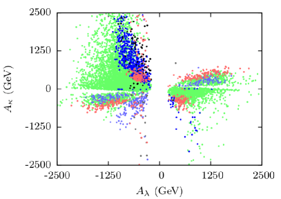
In line with figure 10, we present in figure 14 the the status of the DSB vacuum in the $A_{\lambda}-A_{\kappa}$ plane for the NMSSM-like regime. Similar considerations as discussed in the context of figure 10 apply except for we now have to retain the terms containing the product $v_{d}v_{u}$ in the relevant expressions of equations 15 and 19 and cannot just use their approximated versions presented in equation36. As may be recalled, this is since in the NMSSM-like scenario $\lambda$ is taken to be relatively large thus rendering $v_{{}_{S}}$ to be on the smaller side for a given value of $\mu_{\mathrm{eff}}$. A little algebra with equation 19 then reveals that the magnitude of $A_{\kappa}$ gets quickly bounded from above when one demands the singlet $CP$-odd scalar to be non-tachyonic. Subsequently, an inequality connecting $A_{\kappa}$ and $A_{\lambda}$ can be derived by demanding the $CP$-even singlet scalar to be non-tachyonic as well using equation 15. This reveals that $A_{\lambda}$ also eventually receives an upper bound. The phenomenon is reflected in both plots of figure 14 that correspond to the cases with singlino-like (left) and higgsino-like (right) LSP, respectively. However, such a restriction is more evident in the first (second) and the third (fourth) quadrants with $\kappa<0$ ($\kappa>0$) in the cases with a singlino- (higgsino)-like LSP. Note that a characteristic dependence on $A_{\lambda}$ in the NMSSM-like scenario is in contrast to the MSSM-like case for which the dependence on $A_{\lambda}$ fades out because of large values of $v_{{}_{S}}$. For the case with a singlino-like LSP it is observed that a stable (in green) DSB vacuum appears more frequently for a larger magnitude of $A_{\kappa}$ when $A_{\kappa}<0$. The case with a higgsino-like LSP is rather symmetric in $A_{\lambda}$ and $A_{\kappa}$. In both cases regions having a DSB vacuum with varied stability-status are broadly demarcated.

Figure 15: Same as in figure 11 but for the NMSSM-like scenario.

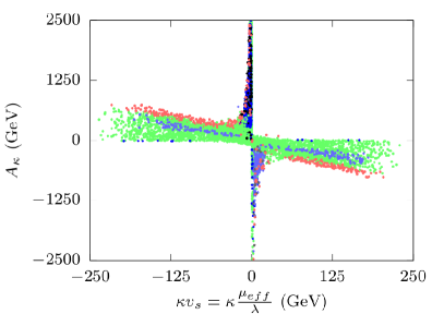
Figure 15 illustrates the results of a Vevacious scan projected on the $\kappa v_{{}_{S}}-A_{\kappa}$ plane for the NMSSM-like case and is the counterpart of figure 11 presented earlier for the MSSM-like case. Along with regions with stable (in green) and thermally unstable (in red) DSB vacua that appear in figure 11, here we also find clean regions where long-lived DSB vacua appear. Furthermore, regions in black (unstable DSB vacuum under tunneling at zero temperature) also appear clearly beyond the red regions. As in the MSSM-like case, here also the agreement with the results from a Mathematica-based scan is rather impressive. The Vevacious scan additionally reveals metastable regions that ultimately qualify for long-lived DSB vacua (the region in blue) and makes clear distinction between the regions in which the DSB vacuum is long-lived and thermally unstable. It can safely be concluded that over a bulk region of the NMSSM-like parameter space, the DSB vacuum turns out to be stable (the global minimum).

We find that, in the present case, the role of $A_{\kappa}$ in (thermally) destabilizing the DSB vacuum is also very prominent. It may be further observed that for cases with a singlino-like LSP, the role of $A_{\kappa}$ is somewhat diluted and a region with a metastable DSB vacuum eventually survive tunneling to a deeper minimum and becomes long-lived. For cases with a higgsino-like LSP, $A_{\kappa}$ has a more active role to play and it renders a good part of the region of metastability to that with unstable DSB vacuum.

It is noteworthy that such a level of agreement could be achieved in practice even when we go beyond the single-field approximation for the potential (that is valid only in the MSSM-like case). This is since both our Mathematica-based analysis and the Vevacious formulation do consider the effects of non-vanishing $H_{d}^{0}$ and $H_{u}^{0}$, though at a varied level of sophistication. An implication of such an agreement is that this now provides a genuine scope (and its credibility) of possible, in-depth probes to such multi-scalar scenarios for their underlying analytical nuances in the study of vacuum stability. This is something which is beyond the scope of Vevacious in its present incarnation.

Figure 16: Same as in figure 12 but for the NMSSM-like scenario.

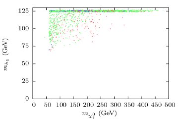
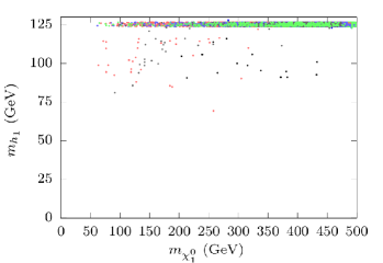
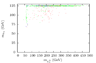
In figure 16 we present the same set of scan-data projected yet again on the $m_{{{}_{\chi}}_{1}^{0}}-m_{h_{1}}$ plane for the cases with singlino-like (left) and higgsino-like (right) LSP. As for figure 12, here also constraints from HiggsBounds and HiggsSignals are included in the plots in the second and the third rows. Furthermore, plots in the second row also receive bounds from the flavor sector. Plots in the third row, in addition, include constraints from the dark matter sector in the form of an upper bound on the relic density as discussed earlier in the context of figure 12. In this case, it is noted that constraints coming from the use of HiggsBounds and HiggsSignals have more drastic effects in the case with a singlino-like LSP. These exclude much of the regions with a long-lived DSB vacuum (in blue) that appear in the plots in the first row. The reason is that for the NMSSM-like scenario $\lambda$ is relatively large and this induces significant mixing between the singlino and the higgsino states in the LSP. This, in turn, results in larger decay rates of the SM-like Higgs boson and the $Z$-boson to a pair of LSP leading to an unacceptable level of invisible widths for them. The sharp edge appearing along an LSP mass of $\sim 60$ GeV is just the kinematic manifestation of the fact that the invisible decay of the SM-like Higgs boson with mass around 125 GeV is totally forbidden as it immediately yields too large an invisible width. Note that this is in clear contrast with the MSSM-like scenario (figure 12) where such a light LSP is a possibility. On the other hand, for the case with higgsino-like LSP, the flavor constraints remove the region with a stable (in green) DSB vacuum appearing for lower values of $m_{h_{1}}$ in the first row. Use of HiggsBounds and HiggsSignals further render the region with a heavier LSP only sparsely populated.

With relatively large $\lambda$ in the NMSSM-like scenario, another associated effect is the enhanced coupling among the SM-like Higgs and a pair of lighter singlet-like Higgs state that might lead to an unacceptable level of decay rate for the SM-like Higgs to the latter states. This results in a (kinematic) edge along $m_{h_{1}}\sim 60$ GeV.

Constraints from the dark matter sector (bottom row) work in a way similar to the MSSM-like scenario in figure 16. Clearly, a thin vertical strand at around $m_{{{}_{\chi}}_{1}^{0}}\sim 62-63$ GeV survives. A palpable depletion in allowed points at moderate value of $m_{{{}_{\chi}}_{1}^{0}}$ is a possible artifact of conspiring parameters that lead to reduced couplings of the LSP to other higgsino-like states thus enhancing the relic density to unacceptable levels.

As far as the the occurrence of a light singlet $CP$-odd scalar is concerned, the considerations are very similar to that in the case of the MSSM-like scenario as dicussed at the end of section 3.3.1 (except for more parameters now entering the picture). The anticorrelation between the masses of the $CP$-odd and $CP$-even singlet scalars in cases with a higgsino-like LSP stil exists. However, in the present case, it is difficult to find an accompanying light (lighter than the SM-like Higgs boson) singlet $CP$-even scalar when its $CP$-odd cousin is light.

4 Charge and color breaking vacua in $Z_{3}$-symmetric NMSSM

In this section we discuss the issue of possible appearance of CCB vacua in the $Z_{3}$-symmetric NMSSM. It may be quickly appreciated that the phenomenon acquires some added degree of intricacy in the presence of the all crucial singlet neutral scalar, when compared to the same in the MSSM. Traditional CCB bounds arise from various combinations of so-called $D$- and $F$-flat directions that now include the colored scalars Ellwanger:1999bv ; Djouadi:2008uj . In the present study we use Vevacious and take a minimal but representative approach by only allowing for the left- and the right-handed top squarks developing vevs. Also, in Vevacious  we consider only one color degree of freedom developing vev at a time.

Generic dangerous directions in the field space, in theories with an extra (singlet) scalar and in the CCB context, have been listed in reference Ellwanger:1999bv . Traditional CCB bounds arise out of negative contribution from some trilinear coupling $A_{ijk}\phi_{i}\phi_{j}\phi_{k}$ where $\phi$-s are the various relevant scalar fields. $D$-flat directions appear along $\phi_{i}=\phi_{j}=\phi_{k}$. Directions flat in both ‘$D$’ and ‘$F$’ are generally the ones along which one comes across a UFB scalar potential. There the improved CCB bounds are also derived in the framework of constrained NMSSM (CNMSSM) along directions other than the above two. These involve non-trivial combinations of uncorrelated field values and exploit the increased number of free parameters in the scenario.

The $D$-flat direction involving the top squarks is given by $|\tilde{t}_{L}|=|\tilde{t}_{R}|=|H_{u}^{0}|$. In the MSSM, CCB minima develop when $A_{t}^{2}>3(m_{{}_{\tilde{t}_{L}}}^{2}+m_{{}_{\tilde{t}_{R}}}^{2}+\hat{m}_{{}_{H_{u}}}^{2})$ and the depth of the minima is of $\mathcal{O}\left({A_{t}^{4}\over y_{t}^{2}}\right)$ Ellwanger:1999bv where $\hat{m}_{{}_{H_{u}}}^{2}=m_{{}_{H_{u}}}^{2}+\mu^{2}$, $A_{t}$ is the trilinear coupling in the top squark sector and $y_{t}$ is the top Yukawa coupling. In the NMSSM, presence of non-vanishing singlet scalar (‘$S$’) turns the minima further deeper to the tune of $\mathcal{O}\left({A_{k}^{4}\over\kappa^{2}}\right)$ Ellwanger:1999bv . Thus, ‘$\kappa$’ and $A_{\kappa}$ take central roles in a study of CCB vacua in the NMSSM. At the same time, it is observed that $\lambda$ and $A_{\lambda}$ affect the proceedings somewhat indirectly. This will become clear as we proceed.

We find that the optimal approach to present the CCB phenomenology is to stick to the broad scenario we adopt in section 3. However, given our present purpose, we choose the parameters in a way such that CCB effects are pronounced, i.e., deeper minima appear along the top squark field direction. This, in general, requires a somewhat larger values of $A_{t}$ and $\tan\beta$. In table 4 we list the set of parameter for various representative scenarios adopted in this study of the CCB vacua.

		Singlino-like LSP	Higgsino-like LSP
MSSM-like	$\lambda$ = 0.05 $\tan\beta$ = 20	$\kappa$ = 0.02	$\kappa$ = 0.10
		-2500 GeV <$A_{\kappa}$ <0	-500 GeV <$A_{\kappa}$ <0
NMSSM-like	$\lambda$ = 0.55 $\tan\beta$ = 10	$\kappa$ = 0.20	$\kappa$ = 0.55
		-1500 GeV <$A_{\kappa}$ <0	-500 GeV <$A_{\kappa}$ <0

Table 4: The fixed input parameters and the ranges of others used in the scan for studying the CCB minima for the MSSM- and NMSSM-like scenarios with a singlino-like and higgsino-like LSP. Throughout, $A_{t}$ is varied over the range $|A_{t}|<7.5$ TeV and we take $\mu_{\mathrm{eff}}=300$ GeV.

In the light of the discussion above, we explore how the stability of the DSB vacua gets affected by changing values of the soft trilinear parameters $A_{t}$, $A_{\kappa}$ and $A_{\lambda}$ and the soft masses of the top squarks. For clarity, we keep other parameters fixed at values representative of the scenarios presented.

Figure 17: Regions obtained from Vevacious scan in the $A_{t}-A_{\kappa}$ plane indicating the fate of the DSB vacuum in the MSSM-like (top panel) and the NMSSM-like (bottom panel) scenarios with a singlino-like (left) and a higgsino-like LSP (right). Color-code used is as summarized in table 3. The fixed and varying input parameters are as shown in table 4.

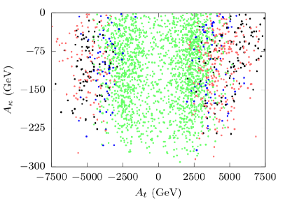
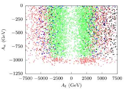
In figure 17 we explore how stable the DSB vacua are in the $A_{t}-A_{\kappa}$ plane for the MSSM-like (top panel) and the NMSSM-like (bottom panel) scenarios and with a singlino-like (left) and higgsino-like (right) LSP. It shows that, for not too large an $A_{\kappa}$, the fate of the DSB vacua is broadly determined by $|A_{t}|$, as is the case in the MSSM. As expected, a smaller $|A_{t}|$ would still leave the DSB minima to be the global ones and thus stable (green points). However, with increasing $|A_{t}|$, the scalar potential develops deeper minima in the direction of top squark field(s). Thus, the DSB vacua become metastable. For an intermediate range of $|A_{t}|$, the tunneling time of the DSB vacuum to a deeper minimum is still long enough thus making the latter long-lived (blue points). Even larger $|A_{t}|$ values, however, render the DSB vacua unstable (black and red points).

The role of $|A_{\kappa}|$ becomes apparent as soon as it becomes larger than a critical value that depends on the case in hand. Such effects are marked by abrupt onset of regions in red at the bottom of (three of) these plots. This can be understood in terms of deeper minima developing in the direction of the singlet scalar field ‘$S$’. Given that the depth of such deeper minima goes as $\mathcal{O}\left({A_{\kappa}^{4}\over\kappa^{2}}\right)$, these minima could get quickly deeper than the ones developed in the top squark direction(s) for smaller values of $\kappa$. Note that, in a given broad scenario (say, the MSSM-like one; the first row) the larger the value of ‘$\kappa$’, the bigger an $|A_{\kappa}|$ is required for the onset of such a deeper minimum in the ‘$S$’ direction. It may also be expected that once there is an onset of such a minimum, increasing $|A_{\kappa}|$ would only render the same even deeper before it reaches the critical value that turns the singlet $CP$-even scalar tachyonic (see equations 15, 33). The expression for the mass of the singlet $CP$-odd scalar in the latter equation and the requirement of this state to be non-tachyonic explain the sign on $A_{\kappa}$ for our choice of $\kappa,\lambda>0$ and $\mu_{\mathrm{eff}}(=\lambda/v_{{}_{S}})>0$.

Figure 18: Same as in figure 17 but in the $A_{t}-A_{\lambda}$ plane.

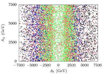
The vertical depletion of points with smaller values of $A_{t}$ can, in general, be understood in terms of not big enough a correction that it provides to the mass of the SM-like Higgs boson, in the MSSM- and NMSSM-like cases alike. For the MSSM-like scenario this is already expected while for the NMSSM-like case this is an artifact of choosing not large enough a value of $\lambda$.

In figure 18 an analogous study is presented in the $A_{t}-A_{\lambda}$ plane. In the MSSM-like scenario with a singlino-like LSP (top panel, left) the issue of stability of the DSB vacuum is almost solely determined by $A_{t}$, i.e., on whether (and what kind of) CCB minima develop. For the MSSM-like scenario with a higgsino-like LSP (top panel, left) the various stability regions are mixed up. Given the scan-range of $A_{\kappa}$ for this case (which includes values giving rise to the thermally unstable (red) region in a similar scenario in figure 17), it may not be difficult to recognize that the red points appearing at small values of $A_{t}$ are not due to deeper CCB minima but because of deeper minima appearing in the ‘$S$’ direction. Also, it may be noted, that stable (green) and long-lived (blue) DSB vacua exist for comparatively smaller $A_{t}$ values. For the NMSSM-like scenario (bottom panel) the stability of the DSB vacua hardly depends on $A_{\lambda}$ and is solely governed by the nature of the CCB minima which in turn depends on $|A_{t}|$. However, some rather sparsely populated red (thermally unstable) regions may be seen in the bottom, right plot which is again due values of $A_{\kappa}$ that lead to deeper minima in the ‘$S$’ direction. We find that with larger values of $\lambda$ in the NMSSM-like scenario it is difficult to obtain the mass of the SM-like Higgs boson in the correct range unless $A_{\lambda}$ is large.

Figure 19 presents the results of Vevacious scan in the familiar $A_{t}-m_{h_{1}}$ plane with varying top squark masses and $A_{t}$ while $A_{\kappa}$ and $A_{\lambda}$ are kept fixed at values shown in its caption. In all the cases (mostly) non-overlapping regions with different kinds of stability property of the DSB vacuum are observed. The choice of $A_{\kappa}=-100$ GeV, as can be gleaned from figure 17, rules out the possibility of development of deeper minima in the ‘$S$’ direction. Thus, the issue of stability of the DSB vacuum exclusively refers to the appearance of deeper CCB minima as $|A_{t}|$ grows and hence should be consistent with the traditional CCB constraints (in the MSSM) Chattopadhyay:2014gfa . Indeed, if we take a close look at these set of plots this is found to be the case.

Figure 19: Same as in figure 17 but in the $A_{t}-m_{h_{1}}$ plane for a fixed value of $A_{\kappa}=-100$ GeV. The values of $A_{\lambda}$ are chosen as follows: $A_{\lambda}=2500\,\mathrm{GeV}\;(500\,\mathrm{GeV})$ for the case with a singlino- (higgsino)-like LSP in the MSSM-like scenario and $A_{\lambda}=2500\,\mathrm{GeV}\;(2000\,\mathrm{GeV})$ for the case with a singlino- (higgsino)-like LSP in the NMSSM-like scenario.

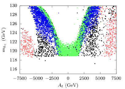
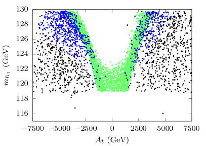
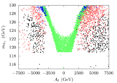
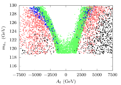
5 Conclusions

In this work we study in detail the occurrence and nature of possible vacua of the $Z_{3}$-symmetric phenomenological NMSSM. The study presented here goes beyond what is available in the existing literature in quite a few aspects.

First, we break away from the fixed (flat) directions in the field space which hitherto were adhered to. We develop a Mathematica-based framework that efficiently deals with the emerging complications when the neutral scalar fields are allowed to vary simultaneously. Furthermore, the study incorporates radiative correction at the 1-loop level to the tree-level neutral scalar potential. Given that it is technically impossible to present a sensible visual map of the terrain of the scalar potential in more than two field dimensions (which is the case here), we illustrate some key features of such a scenario by projecting the potential on suitable slices of low dimensionality. The in-built flexibility of the framework facilitates targeted probe (sometimes purely analytical in nature) and thus, is capable of shedding important light on the intricacies such a system offers. This semi-analytical framework is used further to derive numerical constraints on the free parameters of the scenario.

Second, such an analysis is thoroughly backed up by a detailed scan of the NMSSM parameter space using a dedicated tool like Vevacious. This further includes the thermal correction to the 1-loop effective potential and estimates the stability of the DSB vacuum in the presence of a deeper minimum. This is, to the best of our knowledge, has not previously been considered in the studies of viable vacua of the NMSSM scenarios. The two modes of analyses are thus complimentary in nature; the former helps comprehend the results from the latter with a broad brush while the latter comes up with the state-of-the-art refinements that could factor in all known and applicable, theoretical and experimental constraints from various pertinent sectors of particle physics and cosmology. Nonetheless, there is no denying the fact that the general problem at hand is ultimately one of a hard-core numerical nature. The semi-analytical approach has a limited scope and in practice, feasible when dealing with only a small number of scalar fields.

We carry out our analysis by dividing the NMSSM parameter space into two broad regions based primarily on the magnitude of $\lambda$; a small value of $\lambda$ leads to an ‘MSSM-like’ scenario while a larger value for it results in an ‘NMSSM-like’ one. Furthermore, for a given value of $\mu_{\mathrm{eff}}$, a relatively small ‘$\kappa$’ yields a scenario having a ‘singlino-like’ LSP while for a larger ‘$\kappa$’ one ends up with an LSP which is ‘higgsino-like’. As for the magnitude of $\mu_{\mathrm{eff}}$ is concerned, we confine ourselves to somewhat smaller values for the same and thus settle for $|\mu_{\mathrm{eff}}|<500$ GeV. Such a choice is generally claimed to be friendly to (enhanced) ‘naturalness’ via mitigation of the so-called ‘little hierarchy problem’.

It appears in general that the ‘NMSSM-like’ scenario with a higgsino-like LSP could have absolutely stable DSB vacuum over a large region of parameter space.

Thermal effects are found to play a crucial role in determining the fate of the DSB vacuum. The issue appears to be more important in the MSSM-like case in which had it not been for the thermal contributions, some DSB vacuum configurations would have survived as viable ones. In the MSSM-like scenario, minima deeper than the DSB vacuum that are still safe (thus turning the latter a ‘metastable’ one) arise mostly along the $D$- and $F_{S}$-flat directions in the field space. In the NMSSM-like scenario these appear along other flat directions as well.

With only three neutral scalars allowed to have vevs we find that in the MSSM-like scenario with a higgsino-like LSP, singlet scalars lighter than the SM-Higgs boson are mostly disfavored on the thermal ground. For a situation with a singlino-like LSP in such a scenario, similar restrictions come in for larger values of the LSP mass. On the other hand, in the NMSSM-like scenario with a higgsino-like LSP is the singlet Higgs is prone to be heavier than the SM-like Higgs boson. Attempting to have a lighter singlet-like scalar makes this region thermally inviable. In contrast, since the NMSSM-like scenario with a singlino-like LSP has a comparatively low value of ‘$\kappa$’, finding a somewhat lighter (than the SM-like Higgs boson) singlet scalar is easier by tweaking $A_{\kappa}$. However, this comes with a price. The region with light singlet scalars tend to get metastable but long-lived (short-lived) for lighter (heavier) LSP. We also find that regions with $m_{h_{1}}<{m_{H_{\mathrm{SM}}}\over 2}$ are now experimentally disfavored because of an unacceptably large decay rate for $H_{\mathrm{SM}}\to h_{1}h_{1}$ when $\lambda$ is large.

As far as the CCB sector is concerned, we observe that it is sensitive to $A_{t}$ (as in the MSSM) ‘$\kappa$’ and $A_{\kappa}$ and their interplay. The latter two determine the depth of the minima in the ‘$S$’ direction which may easily surpass the depths of the CCB minima and hence play the all important role in determining the fate of the DSB vacuum. Traditional CCB bounds hold only when $A_{\kappa}$ is on the smaller side. Beyond a critical value which depends upon other free parameters, the dominance of $A_{\kappa}$ sets in. Under its spell, it is mostly the thermal effect that makes the DSB vacuum short-lived.

We find that light singlet scalars are rather common over a significant region of the parameter space of phenomenological interest that is also compatible with a viable DSB vacuum. They can also be accompanied by a light LSP having significant singlino admixture. Hence their search at the LHC would continue to be rather interesting. This usually includes looking for production of a pair of such light scalars (or their production in cascades of heavier particles) followed by their decays to final states with multiple $b$-jets and/or photons and/or leptons.