Singularity-Free Spacecraft Attitude Control Using Variable-Speed Control Moment Gyroscopes

Abstract

This paper discusses spacecraft control using variable-speed CMGs. A new operational concept for VSCMGs is proposed. This new concept makes it possible to approximate the complex nonlinear system by a linear time-varying system (LTV). As a result, an effective control system design method, Model Predictive Control (MPC) using robust pole assignment, can be used to design the spacecraft control system using VSCMGs. A nice feature of this design is that the control system does not have any singular point. A design example is provided. The simulation result shows the effectiveness of the proposed method.

Keywords: Spacecraft attitude control, control moment gyroscopes, reduced quaternion model.

1 Introduction

Control Moment Gyros (CMGs) are an important type of actuators used in spacecraft control because of their well-known torque amplification property [1]. The conventional use of CMG keeps the flywheel spinning in a constant speed, while torques of the CMG are produced by changing the gimbal’s rotational speed [2]. A more complicated operational concept is the so-called variable-speed control gimbal gyros (VSCMG) in which the flywheel’s speed of the CMG is allowed to be changed too. This idea was first proposed by Ford in his Ph.D dissertation [3] where he derived a mathematical model for VSCMGs which is now widely used in literatures. Because of the extra freedom of VSCMG, it can generate torques on a plane perpendicular to the gimbal axis while the conventional CMG can only generate a torque in a single direction at any instant of time [4].

The existing designs of spacecraft control system using CMG or VSCMG rely on the calculation of the desired torques and then determines the VSCMG’s gimbal speed and flywheel speed. This designs have a fundamental problem because there are singular points where the gimbal speed and flywheel speed cannot be found given the desired torques. Extensive literatures focus on this difficulty of implementation in the last few decades, for example, [1, 5, 6, 7, 8] and references therein. Another difficulty associated with the control system design using CMG or VSCMG is that the nonlinear dynamical models for these type of actuators are much more complicated than other types of actuators used for spacecraft attitude control systems. Most proposed designs, for example [2, 4, 5, 9, 10, 11, 12, 13], use Lyapunov stability theory for nonlinear systems. There are two shortcomings of this design method: first, there is no systematic way to find the desired Lyapunov function, and second, the design does not consider the system performance but only stability.

In this paper, we propose a different operational concept for VSCMG: the flywheels of the cluster of the VSCMG do not always spin at high speed, they spin at high speed only when they need to. The same is true for the gimbals. This operational strategy makes the origin (the state variables at zero) an equilibrium point, where a linearized model can be established. Therefore, some mature linear system design methods can be used and system performance can be part of the design by using these linear system design methods. Additional advantages of the proposed operational concept are: (a) energy saving due to normally reduced spin speed of flywheels and gimbals therefore reduction of operational cost, (b) seamless implementation (singularity free) because the control of the spacecraft is achieved by accelerating or decelerating the flywheels and gimbals, therefore, there is no inverse from desired torques to the speeds of the gimbals and flywheels.

It is worthwhile to point out that the linearized model is a linear time-varying (LTV) system. The design methods for linear time-invariant (LTI) systems cannot be directly applied to LTV systems. A popular design method for LTV system is the so-called gain scheduling design method, which has been discussed in several decades, for example, [14, 15, 16, 17]. The basic idea is to fix the time-varying model in a number of “frozen” models and using linear system design method for each of these “frozen” linear time-invariant systems. When the parameters of the LTV system are not in these “frozen” points, interpolation is used to calculate the feedback gain matrix.

Although, gain scheduling design has been proved to be effective for many applications for LTV systems, it has an intrinsic limitation for some time-varying systems which have many independent time-varying variables, which is the case for spacecraft control using VSCMGs. As we will see later that this control system matrices $({\bf A},{\bf B})$ have many independent time-varying parameters and the computation of the gain scheduling design is too much to be feasible. Therefore, we will consider another popular control system design method, the so-called Model Predictive Control (MPC) [18]. According to a theorem in [19], under certain conditions, the closed-loop LTV system designed by MPC method is stable. To meet some of the required stability conditions imposed on the LTV system [19], we propose using the robust pole assignment design [20, 21] for the MPC design.

The remainder of the paper is organized as follows. Section 2 derives the spacecraft model using variable-speed CMG. Section 3 discusses both gain scheduling design and the MPC design method for spacecraft control using variable-speed CMG. This analysis provides a technical basis of selecting the MPC design over gain scheduling design for this problem. Section 4 provides a design example and simulation result. Section 5 is the summary of the conclusions of the paper.

2 Spacecraft model using variable-speed CMG

Throughout the paper, we will repeatedly use a skew-symmetric matrix which is related to the cross product of two vectors. Let ${\bf a}=[a_{1},a_{2},a_{3}]^{{\rm T}}$ and ${\bf b}=[b_{1},b_{2},b_{3}]^{{\rm T}}$ be two three dimensional vectors. We denote a matrix

$${\bf a}^{\times}=\left[\begin{array}[]{ccc}0&-a_{3}&a_{2}\\ a_{3}&0&-a_{1}\\ -a_{2}&a_{1}&0\end{array}\right]$$

such that the cross product of ${\bf a}$ and ${\bf b}$ is equivalent to a matrix and vector multiplication, i.e., ${\bf a}\times{\bf b}={\bf a}^{\times}{\bf b}$.

Assuming that there are $N$ variable-speed CMGs installed in a spacecraft, following the notations of [3], we define a matrix

$${\bf A}_{s}=[{\bf s}_{1},{\bf s}_{2},\ldots,{\bf s}_{N}]$$ (1)

such that the columns of ${\bf A}_{s}$, ${\bf s}_{j}$ ($j=1,\ldots,N$), specify the unit spin axes of the wheels in the spacecraft body frame. Similarly, we define ${\bf A}_{g}=[{\bf g}_{1},{\bf g}_{2},\ldots,{\bf g}_{N}]$ the matrix whose columns are the unit gimbal axes and ${\bf A}_{t}=[{\bf t}_{1},{\bf t}_{2},\ldots,{\bf t}_{N}]$ the matrix whose columns are the unit axes of the transverse (torque) directions, both are represented in the spacecraft body frame. Whereas ${\bf A}_{g}$ is a constant matrix, the matrices ${\bf A}_{s}$ and ${\bf A}_{t}$ depend on the gimbal angles. Let $\boldsymbol{\gamma}=[\gamma_{1},\ldots,\gamma_{N}]^{{\rm T}}\in[0,2\pi]\times\cdots\times[0,2\pi]:=\Pi$ be the vector of $N$ gimbal angles,

$$[\dot{\gamma}_{1},\ldots,\dot{\gamma_{N}}]^{{\rm T}}=\dot{\boldsymbol{\gamma}}:=\boldsymbol{\omega}_{g}=[{\omega}_{g_{1}},\ldots,{\omega}_{g_{N}}]^{{\rm T}}$$ (2)

be the vector of $N$ gimbal speed, then the following relations hold [6] (see Figure 1).

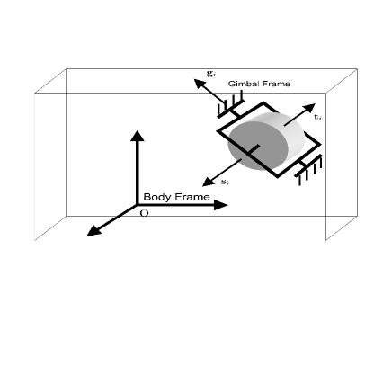
Figure 1: Spacecraft body with a single VSCMG.

$$\dot{{\bf s}}_{i}=\dot{{\gamma}}_{i}{\bf t}_{i}={{\omega}}_{g_{i}}{\bf t}_{i},\hskip 7.22743pt\dot{{\bf t}}_{i}=-\dot{{\gamma}}_{i}{\bf s}_{i}={{\omega}}_{g_{i}}{\bf s}_{i},\hskip 7.22743pt\dot{{\bf g}}_{i}=0.$$ (3)

Denote

$$\boldsymbol{\Gamma}^{c}={\rm diag}(\cos(\boldsymbol{\gamma})),\hskip 7.22743pt\boldsymbol{\Gamma}^{s}={\rm diag}(\sin(\boldsymbol{\gamma})).$$ (4)

A different but related expression is given in [3] . Let ${\bf A}_{s_{0}}$ and ${\bf A}_{t_{0}}$ be initial spin axes and gimbal axes matrices at $\boldsymbol{\gamma_{0}}={\bf 0}$, then

$${\bf A}_{s}(\boldsymbol{\gamma})={\bf A}_{s_{0}}\boldsymbol{\Gamma}^{c}+{\bf A}_{t_{0}}\boldsymbol{\Gamma}^{s},$$ (5a)

$${\bf A}_{t}(\boldsymbol{\gamma})={\bf A}_{t_{0}}\boldsymbol{\Gamma}^{c}-{\bf A}_{s_{0}}\boldsymbol{\Gamma}^{s}.$$ (5b)

This gives

$$\dot{{\bf A}}_{s}={\bf A}_{t_{0}}{\rm diag}(\dot{\boldsymbol{\gamma}})={\bf A}_{t_{0}}{\rm diag}(\boldsymbol{\omega}_{g}),$$ (6a)

$$\dot{{\bf A}}_{t}=-{\bf A}_{s_{0}}{\rm diag}(\dot{\boldsymbol{\gamma}})=-{\bf A}_{s_{0}}{\rm diag}(\boldsymbol{\omega}_{g}),$$ (6b)

which are identical to the formulas of (3). Let $J_{s_{j}}$, $J_{g_{j}}$, and $J_{t_{j}}$ be the spin axis inertia, the gimbal axis inertia, and the transverse axis inertia of the $j$-th CMG, let three $N\times N$ matrices be defined as

$${\bf J}_{s}={\rm diag}(J_{s_{j}}),\hskip 7.22743pt{\bf J}_{g}={\rm diag}(J_{g_{j}}),\hskip 7.22743pt{\bf J}_{t}={\rm diag}(J_{t_{j}}).$$ (7)

Let the spacecraft inertia matrix be ${\bf J}_{b}$, then the total inertia matrix including the CMG clusters is given by [3]

$${\bf J}={\bf J}_{b}+{\bf A}_{s}{\bf J}_{s}{\bf A}_{s}^{{\rm T}}+{\bf A}_{g}{\bf J}_{g}{\bf A}_{g}^{{\rm T}}+{\bf A}_{t}{\bf J}_{t}{\bf A}_{t}^{{\rm T}},$$ (8)

which is a function of $\boldsymbol{\gamma}$, and $\boldsymbol{\gamma}$ is a variable depending of time $t$. Therefore, ${\bf J}$ is an implicit function of time $t$. Although ${\bf J}$ is a function $\boldsymbol{\gamma}$, the dependence of ${\bf J}$ on $\boldsymbol{\gamma}$ is weak, especially when the size of spacecraft main body is large [4]. We therefore assume that $\dot{{\bf J}}=0$ as treated in [9, 10, 11, 12]. Let $\boldsymbol{\omega}=[\omega_{1},\omega_{2},\omega_{3}]^{{\rm T}}$ be the spacecraft body angular rate with respect to the inertial frame, $\boldsymbol{\beta}=[\beta_{1},\ldots,\beta_{N}]^{{\rm T}}$ be the vector of $N$ wheel angles,

$$[\dot{\beta}_{1},\ldots,\dot{\beta}_{N}]^{{\rm T}}=\dot{\boldsymbol{\beta}}:=\boldsymbol{\omega}_{s}=[{\omega}_{s_{1}},\ldots,{\omega}_{s_{N}}]^{{\rm T}}$$ (9)

be the vector of $N$ wheel speed. Denote

$${\bf h}_{s}=[J_{s_{1}}\dot{\beta}_{1},\ldots,J_{s_{N}}\dot{\beta}_{N}]^{{\rm T}}={\bf J}_{s}\boldsymbol{\omega}_{s},$$ (10)

$${\bf h}_{g}=[J_{g_{1}}\dot{\gamma}_{1},\ldots,J_{g_{N}}\dot{\gamma}_{N}]^{{\rm T}}={\bf J}_{g}\boldsymbol{\omega}_{g},$$ (11)

and ${\bf h}_{t}$ be the $N$ dimensional vectors representing the components of absolute angular momentum of the CMGs about their spin axes, gimbal axes, and transverse axes respectively. The total angular momentum of the spacecraft with a cluster of CMGs represented in the body frame is given as

$${\bf h}={\bf J}_{b}\boldsymbol{\omega}+\sum_{i=1}^{N}{\bf s}_{i}J_{s_{i}}\dot{\beta}_{i}+\sum_{i=1}^{N}{\bf g}_{i}J_{g_{i}}\dot{\gamma}_{i}={\bf J}_{b}\boldsymbol{\omega}+{\bf A}_{s}{\bf h}_{s}+{\bf A}_{g}{\bf h}_{g}={\bf J}_{b}\boldsymbol{\omega}+{\bf A}_{s}{\bf J}_{s}\boldsymbol{\omega}_{s}+{\bf A}_{g}{\bf J}_{g}\boldsymbol{\omega}_{g}.$$ (12)

Taking derivative of (12) and using (3) and $\dot{{\bf J}}=0$, noticing that gimbal axes are fixed, we have

$$\dot{{\bf h}} = {\bf J}_{b}\dot{\boldsymbol{\omega}}+\sum_{i=1}^{N}\left(\dot{{\bf s}}_{i}J_{s_{i}}\dot{\beta}_{i}+{{\bf s}_{i}}J_{s_{i}}\ddot{\beta}_{i}\right)+\sum_{i=1}^{N}\left(\dot{{\bf g}}_{i}J_{g_{i}}\dot{\gamma}_{i}+{{\bf g}}_{i}J_{g_{i}}\ddot{\gamma}_{i}\right)$$ (13)

$$= {\bf J}_{b}\dot{\boldsymbol{\omega}}+\sum_{i=1}^{N}\left(\dot{\gamma}_{i}{\bf t}_{i}J_{s_{i}}\dot{\beta}_{i}+{{\bf s}_{i}}J_{s_{i}}\ddot{\beta}_{i}\right)+\sum_{i=1}^{N}{{\bf g}}_{i}J_{g_{i}}\ddot{\gamma}_{i}$$

$$= -{\boldsymbol{\omega}}\times{\bf h}+{\bf t}_{e},$$

where ${\bf t}_{e}$ is the external torque. Denote $\boldsymbol{\Omega}_{s}={\rm diag}(\boldsymbol{\omega}_{s})$ and $\boldsymbol{\Omega}_{g}={\rm diag}(\boldsymbol{\omega}_{g})$. This equation can be written as a compact form as follows.

$${\bf J}_{b}\dot{\boldsymbol{\omega}}+{\bf A}_{t}{\bf J}_{s}\boldsymbol{\Omega}_{s}\boldsymbol{\omega}_{g}+{\bf A}_{s}{\bf J}_{s}\dot{\boldsymbol{\omega}}_{s}+{{\bf A}}_{g}{\bf J}_{g}\dot{\boldsymbol{\omega}}_{g}=-{\boldsymbol{\omega}}\times({\bf J}_{b}\boldsymbol{\omega}+{\bf A}_{s}{\bf J}_{s}\boldsymbol{\omega}_{s}+{\bf A}_{g}{\bf J}_{g}\boldsymbol{\omega}_{g})+{\bf t}_{e},$$ (14)

Note that the torques generated by wheel acceleration or deceleration in the directions defined by ${\bf A}_{s}$ are given by

$${\bf t}_{s}=-{\bf J}_{s}\boldsymbol{\dot{\omega}}_{s}=[t_{s_{1}},\ldots,t_{s_{N}}]^{{\rm T}}$$ (15)

(note that vectors ${\bf t}_{i}$ in ${\bf A}_{t}$ are axes and scalars $t_{s_{i}}$ in ${\bf t}_{s}$ are torques) and the torques generated by gimbal acceleration or deceleration in the directions defined by ${\bf A}_{g}$ are given by

$${\bf t}_{g}=-{\bf J}_{g}\boldsymbol{\dot{\omega}}_{g}=[t_{g_{1}},\ldots,t_{g_{N}}]^{{\rm T}},$$ (16)

the dynamical equation can be expressed as

$${\bf J}_{b}\dot{\boldsymbol{\omega}}+{\bf A}_{t}{\bf J}_{s}\boldsymbol{\Omega}_{s}\boldsymbol{\omega}_{g}+{\boldsymbol{\omega}}\times({\bf J}_{b}\boldsymbol{\omega}+{\bf A}_{s}{\bf J}_{s}\boldsymbol{\omega}_{s}+{\bf A}_{g}{\bf J}_{g}\boldsymbol{\omega}_{g})={\bf A}_{s}{\bf t}_{s}+{{\bf A}}_{g}{\bf t}_{g}+{\bf t}_{e}.$$ (17)

Let

$$\bar{{\bf q}}=[q_{0},q_{1},q_{2},q_{3}]^{{\rm T}}=[q_{0},{\bf q}^{{\rm T}}]^{{\rm T}}=\left[\cos(\frac{\alpha}{2}),\hat{{\bf e}}^{{\rm T}}\sin(\frac{\alpha}{2})\right]^{{\rm T}}$$ (18)

be the quaternion representing the rotation of the body frame relative to the inertial frame, where $\hat{{\bf e}}$ is the unit length rotational axis and $\alpha$ is the rotation angle about $\hat{{\bf e}}$. Therefore, the reduced kinematics equation becomes [22]

$$\left[\begin{array}[]{c}\dot{q}_{1}\\ \dot{q}_{2}\\ \dot{q}_{3}\end{array}\right] = \frac{1}{2}\left[\begin{array}[]{ccc}\sqrt{1-q_{1}^{2}-q_{2}^{2}-q_{3}^{2}}&-q_{3}&q_{2}\\ q_{3}&\sqrt{1-q_{1}^{2}-q_{2}^{2}-q_{3}^{2}}&-q_{1}\\ -q_{2}&q_{1}&\sqrt{1-q_{1}^{2}-q_{2}^{2}-q_{3}^{2}}\\ \end{array}\right]\left[\begin{array}[]{c}\omega_{1}\\ \omega_{2}\\ \omega_{3}\end{array}\right]$$ (28)

$$= {\bf g}(q_{1},q_{2},q_{3},\boldsymbol{\omega}),$$ (29)

or simply

$$\dot{{\bf q}}={\bf g}({\bf q},\boldsymbol{\omega}).$$ (30)

The nonlinear time-varying spacecraft control system model can be written as follows:

$$\left[\begin{array}[]{c}\dot{\boldsymbol{\omega}}\\ \dot{\boldsymbol{\omega}_{s}}\\ \dot{\boldsymbol{\omega}_{g}}\\ \dot{{\bf q}}\end{array}\right] = \left[\begin{array}[]{c}-{\bf J}_{b}^{-1}\left[{\bf A}_{t}{\bf J}_{s}\boldsymbol{\Omega}_{s}\boldsymbol{\omega}_{g}+{\boldsymbol{\omega}}\times({\bf J}_{b}\boldsymbol{\omega}+{\bf A}_{s}{\bf J}_{s}\boldsymbol{\omega}_{s}+{\bf A}_{g}{\bf J}_{g}\boldsymbol{\omega}_{g})\right]\\ {\bf 0}\\ {\bf 0}\\ {\bf g}({\bf q},\boldsymbol{\omega})\end{array}\right]+\left[\begin{array}[]{c}{\bf J}_{b}^{-1}\left({\bf A}_{s}{\bf t}_{s}+{{\bf A}}_{g}{\bf t}_{g}+{\bf t}_{e}\right)\\ -{\bf J}_{s}^{-1}{\bf t}_{s}\\ -{\bf J}_{g}^{-1}{\bf t}_{g}\\ {\bf 0}\end{array}\right]$$ (43)

$$= {\bf F}(\boldsymbol{\omega},\boldsymbol{\omega}_{g},\boldsymbol{\omega}_{s},{\bf q},t)+{\bf G}({\bf t}_{s},{\bf t}_{g},{\bf t}_{e},t),$$ (44)

or simply

$$\dot{{\bf x}}={\bf F}({\bf x},\boldsymbol{\gamma}(t))+{\bf G}({\bf u},{\bf t}_{e},\boldsymbol{\gamma}(t)),$$ (45)

where the state variable vector is ${\bf x}=[{\boldsymbol{\omega}}^{{\rm T}},\boldsymbol{\omega}_{s}^{{\rm T}},\boldsymbol{\omega}_{g}^{{\rm T}},{\bf q}^{{\rm T}}]^{{\rm T}}$, the control variable vector is ${\bf u}=[{\bf t}_{s}^{{\rm T}},{\bf t}_{g}^{{\rm T}}]^{{\rm T}}$, disturbance torque vector is ${\bf t}_{e}$, and ${\bf F}$ and ${\bf G}$ are functions of time $t$ because the parameters of $\boldsymbol{\omega}$, $\boldsymbol{\omega}_{s}$, $\boldsymbol{\omega}_{g}$, ${\bf q}$, ${\bf A}_{s}$ and ${\bf A}_{t}$ are functions of time $t$. The system dimension is $n=2N+6$. The control input dimension is $2N$.

3 Spacecraft attitude control using variable-speed CMG

We consider two design methods for spacecraft attitude control using variable-speed CMGs. But first, we approximate the nonlinear time-varying spacecraft control system model by a linear time-varying spacecraft control system model near the equilibrium point $\boldsymbol{\omega}={\bf 0}$, $\boldsymbol{\omega}_{s}={\bf 0}$, $\boldsymbol{\omega}_{g}={\bf 0}$, and ${\bf q}={\bf 0}$ so that an effective design considering system performance can be carried out using the simplified linear time-varying model. Denote the equilibrium by ${\bf x}_{e}={\bf 0}=[\boldsymbol{\omega}^{{\rm T}},\boldsymbol{\omega}_{s}^{{\rm T}},\boldsymbol{\omega}_{g}^{{\rm T}},{\bf q}^{{\rm T}}]^{{\rm T}}$ and

$${\bf F}_{1}=-{\bf J}_{b}^{-1}\left[{\bf A}_{t}{\bf J}_{s}\boldsymbol{\Omega}_{s}\boldsymbol{\omega}_{g}+{\boldsymbol{\omega}}\times({\bf J}_{b}\boldsymbol{\omega}+{\bf A}_{s}{\bf J}_{s}\boldsymbol{\omega}_{s}+{\bf A}_{g}{\bf J}_{g}\boldsymbol{\omega}_{g})\right],\hskip 7.22743pt{\bf F}_{2}={\bf F}_{3}={\bf 0},\hskip 7.22743pt{\bf F}_{4}={\bf g}({\bf q},\boldsymbol{\omega}),$$ (46)

$${\bf G}_{1}={\bf J}_{b}^{-1}\left({\bf A}_{s}{\bf t}_{s}+{{\bf A}}_{g}{\bf t}_{g}+{\bf t}_{e}\right),\hskip 7.22743pt{\bf G}_{2}=-{\bf J}_{s}^{-1}{\bf t}_{s},\hskip 7.22743pt{\bf G}_{3}=-{\bf J}_{g}^{-1}{\bf t}_{g},\hskip 7.22743pt{\bf G}_{4}={\bf 0}.$$ (47)

Taking partial derivative for ${\bf F}_{1}$, we have

$$\frac{\partial{\bf F}_{1}}{\partial\boldsymbol{\omega}}={\bf J}_{b}^{-1}[({\bf A}_{s}{\bf J}_{s}\boldsymbol{\omega}_{s})^{\times}+({\bf A}_{g}{\bf J}_{g}\boldsymbol{\omega}_{g})^{\times}-\boldsymbol{\omega}^{\times}{\bf J}_{b}+({\bf J}_{b}\boldsymbol{\omega})^{\times}]:={\bf F}_{11},$$ (48)

$$\frac{\partial{\bf F}_{1}}{\partial\boldsymbol{\omega}_{s}}=-{\bf J}_{b}^{-1}[{\bf A}_{t}{\bf J}_{s}\boldsymbol{\Omega}_{g}+\boldsymbol{\omega}^{\times}{\bf A}_{s}{\bf J}_{s}]:={\bf F}_{12},$$ (49)

$$\frac{\partial{\bf F}_{1}}{\partial\boldsymbol{\omega}_{g}}=-{\bf J}_{b}^{-1}[{\bf A}_{t}{\bf J}_{s}\boldsymbol{\Omega}_{s}+\boldsymbol{\omega}^{\times}{\bf A}_{g}{\bf J}_{g}]:={\bf F}_{13},$$ (50)

$$\frac{\partial{\bf F}_{1}}{\partial{\bf q}}={\bf 0}.$$ (51)

Taking partial derivative for ${\bf F}_{4}$, we have

$$\frac{\partial{\bf F}_{4}}{\partial\boldsymbol{\omega}}=\frac{1}{2}\left[\begin{array}[]{ccc}\sqrt{1-q_{1}^{2}-q_{2}^{2}-q_{3}^{2}}&-q_{3}&q_{2}\\ q_{3}&\sqrt{1-q_{1}^{2}-q_{2}^{2}-q_{3}^{2}}&-q_{1}\\ -q_{2}&q_{1}&\sqrt{1-q_{1}^{2}-q_{2}^{2}-q_{3}^{2}}\\ \end{array}\right]_{\begin{subarray}{c}{\bf q}\approx 0\end{subarray}}\approx\frac{1}{2}({\bf I}+{\bf q}^{\times}):={\bf F}_{41},$$ (52)

since $q_{0}=\sqrt{1-q_{1}^{2}-q_{2}^{2}-q_{3}^{2}}$ and $\frac{\partial q_{0}}{\partial q_{i}}=-\frac{q_{i}}{q_{0}}$ for $i=1,2,3$, we have

$$\frac{\partial{\bf F}_{4}}{\partial{\bf q}}=\frac{1}{2}\left[\begin{array}[]{ccc}-\frac{q_{1}}{q_{0}}\omega_{1}&\omega_{3}-\frac{q_{2}}{q_{0}}\omega_{1}&-\omega_{2}-\frac{q_{3}}{q_{0}}\omega_{1}\\ -\omega_{3}-\frac{q_{1}}{q_{0}}\omega_{2}&-\frac{q_{2}}{q_{0}}\omega_{2}&\omega_{1}-\frac{q_{3}}{q_{0}}\omega_{2}\\ \omega_{2}-\frac{q_{1}}{q_{0}}\omega_{3}&-\omega_{1}-\frac{q_{2}}{q_{0}}\omega_{3}&-\frac{q_{3}}{q_{0}}\omega_{3}\end{array}\right]_{\begin{subarray}{c}\boldsymbol{\omega}\approx 0\\ {\bf q}\approx 0\end{subarray}}\approx-\frac{1}{2}\boldsymbol{\omega}^{\times}:={\bf F}_{44}.$$ (53)

Therefore, the linearized time-varying model is given by

$$\left[\begin{array}[]{c}\dot{\boldsymbol{\omega}}\\ \dot{\boldsymbol{\omega}_{s}}\\ \dot{\boldsymbol{\omega}_{g}}\\ \dot{{\bf q}}\end{array}\right] = \left[\begin{array}[]{cccccc}{\bf F}_{11}&{\bf F}_{12}&{\bf F}_{13}&{\bf 0}\\ {\bf 0}&{\bf 0}&{\bf 0}&{\bf 0}\\ {\bf 0}&{\bf 0}&{\bf 0}&{\bf 0}\\ {\bf F}_{41}&{\bf 0}&{\bf 0}&{\bf F}_{44}\\ \end{array}\right]\left[\begin{array}[]{c}{\boldsymbol{\omega}}\\ {\boldsymbol{\omega}_{s}}\\ {\boldsymbol{\omega}_{g}}\\ {{\bf q}}\end{array}\right]+\left[\begin{array}[]{cc}{\bf J}_{b}^{-1}{\bf A}_{s}&{\bf J}_{b}^{-1}{{\bf A}}_{g}\\ -{\bf J}_{s}^{-1}&{\bf 0}\\ {\bf 0}&-{\bf J}_{g}^{-1}\\ {\bf 0}&{\bf 0}\end{array}\right]\left[\begin{array}[]{c}{{\bf t}_{s}}\\ {{\bf t}_{g}}\end{array}\right]+\left[\begin{array}[]{c}{\bf J}_{b}^{-1}\\ {\bf 0}\\ {\bf 0}\\ {\bf 0}\end{array}\right]{{\bf t}_{e}}$$ (76)

$$= {\bf A}{\bf x}+{\bf B}{\bf u}+{\bf C}{\bf t}_{e},$$ (77)

where ${\bf C}$ is a time-invariant matrix. The linearized system is time-varying because ${\boldsymbol{\omega}}$, $\boldsymbol{\omega}_{s}$, $\boldsymbol{\omega}_{g}$, ${\bf q}$, ${\bf A}_{s}$ and ${\bf A}_{t}$ in ${\bf A}$ and ${\bf B}$ are all functions of $t$.

Remark 3.1

It is worthwhile to note that the linearized system matrices ${\bf A}$, ${\bf B}$, and ${\bf C}$ will be time-invariant if we approximate the linear system at the equilibrium point of the origin (${\bf x}_{e}={\bf 0}$). However, such a linear time invariant system will not be controllable. Therefore, we take the first order approximation for ${\bf A}$ and ${\bf B}$, which leads to a controllable linear time-varying system.

In theory, given ${\bf A}_{s_{0}}$, ${\bf A}_{t_{0}}$, and ${\boldsymbol{\omega}_{g}}$, ${\bf A}_{s}$ and ${\bf A}_{t}$ can be calculated by the integration of (6). But using (4) and (5) is a better method because it ensures that the columns of ${\bf A}_{s}$ and ${\bf A}_{t}$ are unit vectors as required. Notice that the $i$th column of ${\bf A}_{s}$ and the $i$th column of ${\bf A}_{t}$, $i=1,\ldots,n$, must be perpendicular to each other, an even better method to update ${\bf A}_{t}$ is to use the cross product

$${\bf t}_{i}={\bf g}_{i}\times{\bf s}_{i},\hskip 7.22743pti=1,\ldots,n,$$ (78)

to prevent ${\bf t}_{i}$ and ${\bf s}_{i}$ from being losing perpendicularity due to the numerical error accumulation. In simulation, integration of (2) can be used to obtain $\boldsymbol{\gamma}$ which is needed in the computation of (4), but in engineering practice, the encoder measurement should be used to get $\boldsymbol{\gamma}$.

Assuming that the closed-loop linear time-varying system is given by

$$\dot{{\bf x}}=\bar{{\bf A}}(t){\bf x}(t),\hskip 7.22743pt{\bf x}(t_{0})={\bf x}_{0}.$$ (79)

It is well-known that even if all the eigenvalues of $\bar{{\bf A}}(t)$, denoted by ${\cal R}_{e}[\lambda(t)]$, are in the left half complex plane for all $t$, the system may not be stable [19, pages 113-114]. But the following theorem (cf. [19, pages 117-119]) provides a nice stability criterion for the closed-loop system (79).

Theorem 3.1

Suppose for the linear time-varying system (79) with $\bar{{\bf A}}(t)$ continuously differentiable there exist finite positive constants $\alpha$, $\mu$ such that, for all $t$, $\|\bar{{\bf A}}(t)\|\leq\alpha$ and every point-wise eigenvalue of $\bar{{\bf A}}(t)$ satisfies ${\cal R}_{e}[\lambda(t)]\leq-\mu$. Then there exists a positive constant $\beta$ such that if the time derivative of $\bar{{\bf A}}(t)$ satisfies $\|\dot{\bar{{\bf A}}}(t)\|\leq\beta$ for all $t$, the state equation is uniformly exponentially stable.

This theorem is the theoretical base for the linear time-varying control system design. We need at least that ${\cal R}_{e}[\lambda(t)]\leq-\mu$ holds.

3.1 Gail scheduling control

Gain scheduling control design is fully discussed in [14] and it seems to be applicable to this LTV system. The main idea of gain scheduling is: 1) select a set of fixed parameters’ values, which represent the range of the plant dynamics, and design a linear time-invariant gain for each; and 2) in between operating points, the gain is interpolated using the designs for the fixed parameters’ values that cover the operating points. As an example, for $i=1,\ldots,N$, let $\gamma_{i}\in\{2\pi/p_{\gamma},4\pi/p_{\gamma},\cdots,2\pi\}$ be a set of $p_{\gamma}$ fixed points equally spread in $[0,2\pi]$. Then, for $N$ CMGs, there are $p_{\gamma}^{N}$ possible fixed parameters’ combinations. For example, if $N=4$ and $p_{\gamma}=8$, we can represent the grid composed of these fixed points in a matrix form as follows:

$$\left[\begin{array}[]{cccccccc}\pi/4&\pi/2&3\pi/4&\pi&5\pi/4&3\pi/2&7\pi/4&2\pi\\ \pi/4&\pi/2&3\pi/4&\pi&5\pi/4&3\pi/2&7\pi/4&2\pi\\ \pi/4&\pi/2&3\pi/4&\pi&5\pi/4&3\pi/2&7\pi/4&2\pi\\ \pi/4&\pi/2&3\pi/4&\pi&5\pi/4&3\pi/2&7\pi/4&2\pi\end{array}\right],$$ (80)

and each fixed $\boldsymbol{\gamma}$ is a vector composed of $\gamma_{i}$ ($i=1,2,3,4$) which can be any element of $i$th row. If $\boldsymbol{\gamma}$ is not a fixed point, we have $\gamma_{i}\in[\kappa(i),\kappa(i)+1]$ for all $i\in[1,\cdots,N-1]$. Assume that $\gamma_{i}$ is in the interior of $(\kappa(i),\kappa(i)+1)$ for all $i\in[1,\cdots,N-1]$. Then, $\boldsymbol{\gamma}$ meets the following conditions:

$$\boldsymbol{\gamma}=\left[\begin{array}[]{c}\gamma_{1}\in(\kappa(1),\kappa(1)+1)\\ \vdots\\ \gamma_{N}\in(\kappa(N),\kappa(N)+1)\end{array}\right].$$ (81)

Using the previous example of (80), if $\boldsymbol{\gamma}=\left[\frac{5\pi}{8},\frac{3\pi}{8},\frac{7\pi}{16},\frac{15\pi}{8}\right]^{{\rm T}}$, then $\boldsymbol{\gamma}\in\left[(\frac{\pi}{2},\frac{3\pi}{4}),(\frac{\pi}{4},\frac{\pi}{2}),(\frac{\pi}{4},\frac{\pi}{2}),(\frac{7\pi}{4},{2\pi})\right]^{{\rm T}}$. To use gain scheduling control, we need also to consider fixed points for ${\boldsymbol{\omega}}$, $\boldsymbol{\omega}_{s}$, $\boldsymbol{\omega}_{g}$, and ${\bf q}$ in their possible operational ranges. Let $p_{w}$, $p_{w_{s}}$, $p_{w_{g}}$, and $p_{q}$ be the number of the fixed points for ${\boldsymbol{\omega}}$, $\boldsymbol{\omega}_{s}$, $\boldsymbol{\omega}_{g}$, and ${\bf q}$. The total vertices for the entire polytope (including a grid of all possible time-varying parameters) will be $p_{\gamma}^{N}p_{w}^{3}p_{w_{s}}^{N}p_{w_{g}}^{N}p_{q}^{3}$.

For each of these ($p_{\gamma}^{N}p_{w}^{3}p_{w_{s}}^{N}p_{w_{g}}^{N}p_{q}^{3}$) fixed models, we need conduct a control design to calculate the feedback gain matrix for the “frozen” model. If the system (77) at time $t$ happens to have all parameters equal to the fixed points, we can use a “frozen” feedback gain to control the system (77). Otherwise, we need to construct a gain matrix based on $2^{3N+6}$ “frozen” gain matrices. Assuming that each parameter has some moderate number of fixed points, say $8$, and the control system has $N=4$ gimbals, the total number of the fixed models will be $8^{18}$, each needs to compute a feedback matrix, an impossibly computational task.

3.2 Model Predictive Control

Unlike the gain scheduling control design in which most computation is done off-line, model predictive control computes the feedback gain matrix on-line for the linear system (77) in which ${\bf A}$ and ${\bf B}$ matrices are updated in every sampling period. It is straightforward to verify that for any given $\boldsymbol{\gamma}$, if ${\bf x}\neq{\bf x}_{e}$, the linear system (77) is controllable. In theory, one can use either robust pole assignment [20, 21], or LQR design [23], or ${\bf H}_{\infty}$ design [24] for the on-line design, but ${\bf H}_{\infty}$ design costs significant more computational time and should not be considered for this on-line design problem. Since LTV system design should meet the condition of ${\cal R}_{e}[\lambda(t)]\leq-\mu$ required in Theorem 3.1, robust pole assignment design is clearly a better choice than LQR design for this purpose. Another attrictive feature of the robust pole assignment design is that the perturbation of the closed loop eigenvalues between sampling period are expected to be small. It is worthwhile to note that a robust pole assignment design [21] minimizes an upper bound of ${\bf H}_{\infty}$ norm which means that the design is robust to the modeling error and reduces the impact of disturbance torques on the system output [25, 26]. Additional merits about this method, such as computational speed which is important for the on-line design, is discussed in [27]. Therefore, we use the method of [21] in the proposed design.

The proposed design algorithm is given as follows:

Algorithm 3.1

Data: ${\bf J}_{b}$, ${\bf J}_{s}$, ${\bf J}_{g}$, and ${\bf A}_{g}$.      
Initial condition: ${\bf x}={\bf x}_{0}$, $\boldsymbol{\gamma}=\boldsymbol{\gamma}_{0}$, ${\bf A}_{s_{0}}$, and ${\bf A}_{t_{0}}$.  

• Step 1: Update ${\bf A}$ and ${\bf B}$ based on the latest $\boldsymbol{\gamma}$ and ${\bf x}$.

• Step 2: Calculate the gain ${\bf K}$ using robust pole assignment algorithm robpole (cf. [21]).

• Step 3: Apply feedback ${\bf u}={\bf K}{\bf x}$ to (44) or (77).

• Step 4: Update $\boldsymbol{\gamma}$ and ${\bf x}=[{\boldsymbol{\omega}}^{{\rm T}},\boldsymbol{\omega}_{s}^{{\rm T}},\boldsymbol{\omega}_{g}^{{\rm T}},{\bf q}^{{\rm T}}]^{{\rm T}}$. Go back to Step 1.

4 Simulation test

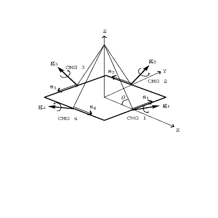
Figure 2: VSCMG system with pyramid configuration concept.

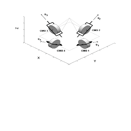
Figure 3: VSCMG system with pyramid configuration.

The proposed design method is simulated using the data in [2, 6, 9]. We assume that the four variable-speed CMGs are mounted in pyramid configuration as shown in Figures 2 and 3. The angle of each pyramid side to its base is $\theta=54.75$ degree; the inertia matrix of the spacecraft is given by [9] as

$${\bf J}_{b}=\left[\begin{array}[]{ccc}15053&3000&-1000\\ 3000&6510&2000\\ -1000&2000&11122\end{array}\right]\hskip 7.22743pt\mbox{kg}\cdot m^{2}.$$ (82)

The spin axis inertial matrix is given by ${\bf J}_{s}={\rm diag}(0.7,0.7,0.7,0.7)\hskip 2.8903pt\mbox{kg}\cdot m^{2}$ and the gimbal axis inertia matrix is given by ${\bf J}_{g}={\rm diag}(0.1,0.1,0.1,0.1)\hskip 2.8903pt\mbox{kg}\cdot m^{2}$. The initial wheel speeds are $2\pi$ radians per second for all wheels. The initial gimbal speeds are all zeros. The initial spacecraft body rate vector is randomly generated by Matlab $rand(3,1)*10^{-3}$ and the initial spacecraft attitude vector is a reduced quaternion randomly generated by Matlab $rand(3,1)*10^{-1}$. The gimbal axis matrix is fixed and given by [6] (cf. Figures 2 and 3.)

$${\bf A}_{g}=\left[\begin{array}[]{cccc}\sin(\theta)&0&-\sin(\theta)&0\\ 0&\sin(\theta)&0&-\sin(\theta)\\ \cos(\theta)&\cos(\theta)&\cos(\theta)&\cos(\theta)\end{array}\right]$$ (83)

The initial wheel axis matrix can be obtained using Figures 2 and 3 and is given by

$${\bf A}_{s}=\left[\begin{array}[]{cccc}0&-1&0&1\\ 1&0&-1&0\\ 0&0&0&0\end{array}\right]$$ (84)

The initial transverse matrix ${\bf A}_{t}$ can be obtained by the method of (78). The desired or designed closed-loop poles are selected as $\{-0.2-0.8,-0.2\pm 0.1i,-0.6\pm 0.1i,-1.5\pm i,-1.6\pm i,-1.7\pm i,-1.8\pm i\}$. The simulation test results are given in Figures 4-7. Clearly, the designed controller stabilizes the system with good performance.

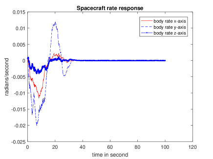
Figure 4: Spacecraft body rate response.

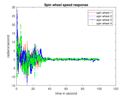
Figure 5: Spin wheel response.

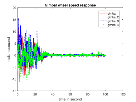
Figure 6: Gimbal wheel response.

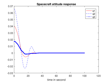
Figure 7: Reaction wheel response $\Omega_{1}$, $\Omega_{2}$, and $\Omega_{3}$.

5 Conclusions

In this paper, we proposed a new operational concept for variable-speed CMGs. This new concept allows us to simplify the nonlinear model of the spacecraft attitude control using variable-speed CMGs to a linear time-varying model. Although this LTV model is significantly simpler than the original nonlinear model, there are still many time-varying parameters in the simplified model. Two LTV control system design methods, the gain scheduling design and model predictive control design, are investigated. The analysis shows that model predictive control is better suited for spacecraft control using variable-speed CMGs. An efficient robust pole assignment algorithm is used in the on-line feedback gain matrix computation. Simulation test demonstrated the effectiveness of the new concept and control system design method.

References

- [1] H. Kurodawa, A geometric study of single gimbal control moment gyros, Report of Mechanical Engineering Laboratory, No. 175, p.108, 1998.
- [2] D. Jung, and P. Tsiotras, An experimental comparison of CMG steering control laws. Collection of Technical Papers-AIAA/AAS Astrodynamics Specialist Conference. Vol. 2. 2004.
- [3] K. A. Ford, Reorientations of flexible spacecraft using momentum exchange devices. No. AFIT/DS/ENG/97-07. Air Force Institute of Technology, Wright-Patterson, OH, 1997.
- [4] H. Yoon, and P. Tsiotras, Spacecraft line-of-sight control using a single variable-speed control moment gyro, Journal of guidance, control, and dynamics, 29(6), 2006, pp.1295-1308.
- [5] K.A. Ford, and C.D. Hall, Singular direction avoidance steering for control-moment gyros, Journal of Guidance, Control, and Dynamics, 23(4), 2000, pp.648-656.
- [6] H. Yoon and P. Tsiotras, Singularity analysis of variable-speed control moment gyros, Journal of Guidance, Control, and Dynamics, 27(3), 2004, pp.374-386.
- [7] H. Kurokawa, Survey of Theory and Steering Laws of Single-Gimbal Control Moment Gyros”, Journal of Guidance, Control, and Dynamics, Vol. 30, No. 5, 2007, pp. 1331-1340.
- [8] J. Zhang, K. Ma, G. Meng, S. Tian, Spacecraft maneuvers via singularity-avoidance of control moment gyros based on dual-mode model predictive control, IEEE Transactions on Aerospace and Electronic Systems 51, 2015, pp. 2546-2559.
- [9] H. Yoon and P. Tsiotras, Spacecraft adaptive attitude and power tracking with variable speed control moment gyroscopes, Journal of Guidance, Control, and Dynamics, 25(6), 2002, pp.1081-1090.
- [10] K.A. Ford, and C.D. Hall, Flexible spacecraft reorientations using gimbal momentum wheels, Advances in the Astronautical Sciences, Astrodynamics, edited by F. Hoots, B. Kaufman, P.J. Cefola, and D.B. Spencer, Vol. 97, Univelt, San Diego, 1997, pp. 1895-1914.
- [11] H. Schaub, S. Vadali, and J.L. Junkins, Feedback control law for variable speed control moment gyroscopes, Journal of the Astronautical Sciences, 46(3), 1998, pp.307-328.
- [12] M.S.I. Malik, and S. Asghar, Inverse free steering law for small satellite attitude control and power tracking with VSCMGs, Advances in Space Research 53, 2013, pp. 97-109.
- [13] J. Jin, and I. Hwang, Attitude Control of a Spacecraft with Single Variable-Speed Control Moment Gyroscope, Journal of Guidance, Control, and Dynamics, Vol. 34, No. 6, 2011, pp. 1920-1925.
- [14] W.J. Rugh, Analytical Framework for Gain Scheduling, American Control Conference, pp. 1688-1694, 23-25 May,San Diego, CA, USA 1990.
- [15] W.J. Rugh, and J.S. Shamma, Research on gain scheduling, Automatica, 36, 2000, pp. 1401-1425.
- [16] D. A. Lawrence and W. J. Rugh, On a Stability Theorem for Nonlinear Systems with Slowly Varying Inputs, IEEE Transactions on Automatic Control, Vol. 35, 1990, pp. 860-864.
- [17] S.M. Shahruz and S. Behtash, Design of controllers for linear parameter-varying systems by the gain scheduling technique, Journal of Mathematical Analysis and Applications, 168(1), pp. 195-217, 1992.
- [18] K.J. Astrom and B. Wittenmark. Computer-controlled systems: theory and design. Courier Corporation, 2013.
- [19] W.J. Rugh, Linear System Theory, Prentice-Hall, Inc., Englewood Cliffs, New Jersey, 1993, pp.117-119.
- [20] Y. Yang, and A.L. Tits, On robust pole assignment by state feedback, Proceedings of the American Control Conference, 1993, pp. 2765-2766.
- [21] A.L. Tits, and Y. Yang, Globally convergent algorithms for robust pole assignment by state feedback, IEEE Transactions on Automatic Control, Vol. 41, 1996, pp. 1432-1452.
- [22] Y. Yang, Quaternion based model for momentum biased nadir pointing spacecraft, Aerospace Science and Technology, 14(3), 199-202, 2010.
- [23] F.L. Lewis, D. Vrabie, and V.L. Syrmos, Optimal Control, 3rd Edition, John Wiley & Sons, Inc., New York, USA, 2012.
- [24] K. Zhou, J.C. Doyle, and K. Glover, Robust and Optimal Control, Prentice Hall, Inc., New Jersey, 1996.
- [25] Y. Yang, Robust System Design: Pole Assignment Approach, University of Maryland at College Park, College Park, MD, December, 1996.
- [26] Y. Yang, Quaternion based LQR spacecraft control design is a robust pole assignment design, Journal of Aerospace Engineering, 27(1), pp. 168-176. 2014.
- [27] A. Pandey, R. Schmid, T. Nguyen,Y. Yang, V. Sima and A. L. Tits, Performance Survey of Robust Pole Placement Methods, the 53rd IEEE Conference on Decision and Control, Los Angeles, December 15-17, 2014.