EUROPEAN ORGANIZATION FOR NUCLEAR RESEARCH (CERN)

​​​ CERN-EP-2016-301 LHCb-PAPER-2016-045

Measurement of the phase difference between short- and long-distance amplitudes in the ${{B}^{+}}\!\rightarrow{{K}^{+}}{\mu^{+}\mu^{-}}$ decay

The LHCb collaboration

A measurement of the phase difference between the short- and long-distance contributions to the ${{B}^{+}}\!\rightarrow{{K}^{+}}{\mu^{+}\mu^{-}}$ decay is performed by analysing the dimuon mass distribution. The analysis is based on $pp$ collision data corresponding to an integrated luminosity of 3$\mbox{\,fb}^{-1}$ collected by the LHCb experiment in 2011 and 2012. The long-distance contribution to the ${{B}^{+}}\!\rightarrow{{K}^{+}}{\mu^{+}\mu^{-}}$ decay is modelled as a sum of relativistic Breit–Wigner amplitudes representing different vector meson resonances decaying to muon pairs, each with their own magnitude and phase. The measured phases of the ${J\mskip-3.0mu/\mskip-2.0mu\psi\mskip 2.0mu}$ and $\psi{(2S)}$ resonances are such that the interference with the short-distance component in dimuon mass regions far from their pole masses is small. In addition, constraints are placed on the Wilson coefficients, $\mathcal{C}_{9}$ and $\mathcal{C}_{10}$, and the branching fraction of the short-distance component is measured.

Published in Eur. Phys. J. C

© CERN on behalf of the LHCb collaboration, licence CC-BY-4.0.

 

1 Introduction

The decay ${{B}^{+}}\!\rightarrow{{K}^{+}}{\mu^{+}\mu^{-}}$ receives contributions from short-distance ${b}\!\rightarrow{s}{\ell^{+}}{\ell^{-}}$ flavour-changing neutral-current (FCNC) transitions and long-distance contributions from intermediate hadronic resonances. In the Standard Model (SM), FCNC transitions are forbidden at tree level and must occur via a loop-level process. In many extensions of the SM, new particles can contribute to the amplitude of the ${b}\!\rightarrow{s}{\ell^{+}}{\ell^{-}}$ process changing the rate of the decay or the distribution of the final-state particles. Decays like ${{B}^{+}}\!\rightarrow{{K}^{+}}{\mu^{+}\mu^{-}}$ are therefore sensitive probes of physics beyond the SM.

Recent global analyses of measurements involving ${b}\!\rightarrow{s}{\ell^{+}}{\ell^{-}}$ processes report deviations from SM predictions at the level of four standard deviations [1, 2, 3, 4, 5, 6, 7, 8, 9, 10, 11, 12, 13, 14, 15]. These differences could be explained by new short-distance contributions from non-SM particles [1, 2, 3, 5, 4, 12, 16] or could indicate a problem with existing SM predictions [17, 15, 13]. To explain the observed tensions, long-distance effects would need to be sizeable in dimuon mass regions far from the pole masses of the resonances. Therefore, it is important to understand how well these long-distance effects are modelled in the SM and how they interfere with the short-distance contributions. Previous measurements of ${b}\!\rightarrow{s}{\ell^{+}}{\ell^{-}}$ processes [18, 19, 20, 21, 22, 23] excluded regions of dimuon mass around the $\phi$, ${J\mskip-3.0mu/\mskip-2.0mu\psi\mskip 2.0mu}$ and $\psi{(2S)}$ resonances. The amplitude in these mass regions is dominated by the narrow vector resonances and has a large theoretical uncertainty. These dimuon regions are therefore considered insensitive to new physics effects.

In this paper, a first measurement of the phase difference between the contributions to the short-distance and the narrow-resonance amplitudes in the ${{B}^{+}}\!\rightarrow{{K}^{+}}{\mu^{+}\mu^{-}}$ decay is presented. For the first time, the branching fraction of the short-distance component is determined without interpolation across the ${J\mskip-3.0mu/\mskip-2.0mu\psi\mskip 2.0mu}$ and $\psi{(2S)}$ regions. The measurement is performed through a fit to the full dimuon mass spectrum, $m_{\mu\mu}$, using a model describing the vector resonances as a sum of relativistic Breit–Wigner amplitudes. This approach is similar to that of Refs. [24, 13], with the difference that the magnitudes and phases of the resonant amplitudes are determined using the LHCb data rather than using the external information on the cross-section for ${e^{+}}{e^{-}}\!\rightarrow{\rm hadrons}$ from the BES collaboration [25]. The model includes the $\rho$, $\omega$, $\phi$, ${J\mskip-3.0mu/\mskip-2.0mu\psi\mskip 2.0mu}$ and $\psi{(2S)}$ resonances, as well as broad charmonium states ($\psi(3770)$, $\psi(4040)$, $\psi(4160)$ and $\psi(4415)$) above the open charm threshold. Evidence for the $\psi(4160)$ resonance in the dimuon spectrum of ${{B}^{+}}\!\rightarrow{{K}^{+}}{\mu^{+}\mu^{-}}$ decays has been previously reported by LHCb in Ref. [26]. The continuum of broad states with pole masses above the maximum $m_{\mu\mu}$ value allowed in the decay is neglected.

The measurement presented in this paper is performed using a data set corresponding to 3$\mbox{\,fb}^{-1}$ of integrated luminosity collected by the LHCb experiment in $pp$ collisions during 2011 and 2012 at $\sqrt{s}$ = 7$\mathrm{\,Te\kern-1.00006ptV}$ and 8$\mathrm{\,Te\kern-1.00006ptV}$. The paper is organised as follows: Section 2 describes the LHCb detector and the procedure used to generate simulated events; the reconstruction and selection of ${{B}^{+}}\!\rightarrow{{K}^{+}}{\mu^{+}\mu^{-}}$ decays are described in Sec. 3; Section 4 describes the $m_{\mu\mu}$ distribution of ${{B}^{+}}\!\rightarrow{{K}^{+}}{\mu^{+}\mu^{-}}$ decays, including the model for the various resonances appearing in the dimuon mass spectrum; the fit procedure to the dimuon mass spectrum, including the methods to correct for the detection and selection biases, is discussed in Sec. 5. The results and associated systematic uncertainties are discussed in Secs. 6 and 7. Finally, conclusions are presented in Sec. 8.

2 Detector and simulation

The LHCb detector [27, 28] is a single-arm forward spectrometer, covering the pseudorapidity range $2<\eta<5$, designed to study the production and decay of particles containing $b$ or $c$ quarks. The detector includes a high-precision tracking system divided into three subsystems: a silicon-strip vertex detector surrounding the $pp$ interaction region, a large-area silicon-strip detector that is located upstream of a dipole magnet with a bending power of about $4{\mathrm{\,Tm}}$, and three stations of silicon-strip detectors and straw drift tubes situated downstream of the magnet. The tracking system provides a measurement of the momentum, $p$, of charged particles with a relative uncertainty that varies from 0.5% at low momentum to 1.0% at 200${\mathrm{\,Ge\kern-1.00006ptV\!/}c}$. The momentum scale of tracks in the data is calibrated using the ${{B}^{+}}$ and ${J\mskip-3.0mu/\mskip-2.0mu\psi\mskip 2.0mu}$ masses measured in ${{{B}^{+}}}\!\rightarrow{{J\mskip-3.0mu/\mskip-2.0mu\psi\mskip 2.0mu}}{{K}^{+}}$ decays [29]. The minimum distance of a track to a primary vertex (PV), the impact parameter (IP), is measured with a resolution of $(15+29/\mbox{$p_{\mathrm{T}}$}){\,\upmu\mathrm{m}}$, where $p_{\mathrm{T}}$ is the component of the momentum transverse to the beam, in ${\mathrm{\,Ge\kern-1.00006ptV\!/}c}$. Different types of charged hadrons are distinguished using information from two ring-imaging Cherenkov detectors (RICH). Photons, electrons and hadrons are identified by a calorimeter system consisting of scintillating-pad and preshower detectors, an electromagnetic calorimeter and a hadronic calorimeter. Muons are identified by a system composed of alternating layers of iron and multiwire proportional chambers. The online event selection is performed by a trigger [30], which consists of a hardware stage, based on information from the calorimeter and muon systems, followed by a software stage, which applies a full event reconstruction.

A large sample of simulated events is used to determine the effect of the detector geometry, trigger, and selection criteria on the dimuon mass distribution of the ${{B}^{+}}\!\rightarrow{{K}^{+}}{\mu^{+}\mu^{-}}$ decay. In the simulation, $pp$ collisions are generated using Pythia 8 [31, *Sjostrand:2007gs] with a specific LHCb configuration [33]. The decay of the ${{B}^{+}}$ meson is described by EvtGen [34], which generates final-state radiation using Photos [35]. As described in Ref. [36], the Geant4 toolkit [37, *Agostinelli:2002hh] is used to implement the interaction of the generated particles with the detector and its response. Data-driven corrections are applied to the simulation following the procedure of Ref. [23]. These corrections account for the small level of mismodelling of the detector occupancy, the ${{{B}^{+}}}$ momentum and vertex quality, and the particle identification (PID) performance. The momentum of every reconstructed track in the simulation is also smeared by a small amount in order to better match the mass resolution of the data.

3 Selection of signal candidates

In the trigger for the 7$\mathrm{\,Te\kern-1.00006ptV}$ (8$\mathrm{\,Te\kern-1.00006ptV}$) data, at least one of the muons is required to have $\mbox{$p_{\mathrm{T}}$}>1.48{\mathrm{\,Ge\kern-1.00006ptV\!/}c}$ ($\mbox{$p_{\mathrm{T}}$}>1.76{\mathrm{\,Ge\kern-1.00006ptV\!/}c}$) and one of the final-state particles is required to have both $\mbox{$p_{\mathrm{T}}$}>1.4{\mathrm{\,Ge\kern-1.00006ptV\!/}c}$ ($\mbox{$p_{\mathrm{T}}$}>1.6{\mathrm{\,Ge\kern-1.00006ptV\!/}c}$) and an ${\rm IP}>100{\,\upmu\mathrm{m}}$ with respect to all PVs in the event; if this final-state particle is identified as a muon, $\mbox{$p_{\mathrm{T}}$}>1.0{\mathrm{\,Ge\kern-1.00006ptV\!/}c}$ is required instead. Finally, the tracks of two or more of the final-state particles are required to form a vertex that is significantly displaced from all PVs.

In the offline selection, signal candidates are built from a pair of oppositely tracks that are identified as muons. The muon pair is then combined with a charged track that is identified as a kaon by the RICH detectors. The signal candidates are required to pass a set of loose preselection requirements that are identical to those described in Ref. [26]. These requirements exploit the decay topology of ${{B}^{+}}\!\rightarrow{{K}^{+}}{\mu^{+}\mu^{-}}$ transitions and restrict the data sample to candidates with good-quality vertex and track fits. Candidates are required to have a reconstructed ${{K}^{+}}{\mu^{+}\mu^{-}}$ mass, $m_{K\mu\mu}$, in the range $5100<m_{K\mu\mu}<6500{\mathrm{\,Me\kern-1.00006ptV\!/}c^{2}}$.

Combinatorial background, where particles from different decays are mistakenly combined, is further suppressed with the use of a Boosted Decision Tree (BDT) [39, 40] using kinematic and geometric information. The BDT is identical to that described in Ref. [26] and uses the same working point. The efficiency of the BDT for signal is uniform with respect to $m_{K\mu\mu}$.

Specific background processes can mimic the signal if their final states are misidentified or partially reconstructed. The requirements described in Ref. [26] reduce the overall contribution of the background from such decay processes to a level of less than 1% of the expected signal yield in the full mass region. The largest remaining specific background contribution comes from ${{{B}^{+}}}\!\rightarrow{{\pi}^{+}}{\mu^{+}\mu^{-}}$ decays (including ${{{B}^{+}}}\!\rightarrow{{J\mskip-3.0mu/\mskip-2.0mu\psi\mskip 2.0mu}}{{\pi}^{+}}$ and ${{{B}^{+}}}\!\rightarrow{\psi{(2S)}}{{\pi}^{+}}$), where the pion is mistakenly identified as a kaon.

The ${{K}^{+}}{\mu^{+}\mu^{-}}$ mass of the selected candidates is shown in Fig. 1. The signal is modelled by the sum of two Gaussian functions and a Gaussian function with power-law tails on both sides of the peak; these all share a common peak position. A Gaussian function is used to describe a small contribution from ${B}_{c}^{+}$ decays around the known ${B}_{c}^{+}$ mass [41]. Combinatorial background is described by an exponential function with a negative gradient. At low $m_{K\mu\mu}$, the background is dominated by partially reconstructed $b$-hadron decays, e.g. from $B^{\{+,0\}}\!\rightarrow K^{*\{+,0\}}{\mu^{+}\mu^{-}}$ decays in which the pion from the $K^{*\{+,0\}}$ is not reconstructed. This background component is modelled using the upper tail of a Gaussian function. The shape of the background from ${{{B}^{+}}}\!\rightarrow{{\pi}^{+}}{\mu^{+}\mu^{-}}$ decays is taken from a sample of simulated events. Integrating the signal component in a $\pm 40$${\mathrm{\,Me\kern-1.00006ptV\!/}c^{2}}$ window about the known ${{B}^{+}}$ mass [41] yields 980 000 ${{{B}^{+}}}\!\rightarrow{{K}^{+}}{\mu^{+}}{\mu^{-}}$ decays.

When computing $m_{\mu\mu}$, a kinematic fit is performed to the selected candidates. In the fit, the $m_{K\mu\mu}$ mass is constrained to the known ${{B}^{+}}$ mass and the candidate is required to originate from one of the PVs in the event. For simulated ${{{B}^{+}}}\!\rightarrow{{J\mskip-3.0mu/\mskip-2.0mu\psi\mskip 2.0mu}}{{K}^{+}}$ decays, this improves the resolution in $m_{\mu\mu}$ by about a factor of two.

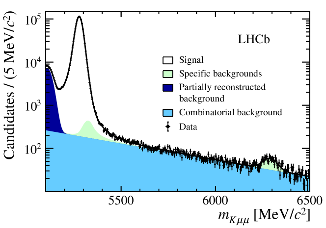
Figure 1: Reconstructed ${{K}^{+}}{\mu^{+}\mu^{-}}$ mass of the selected ${{{B}^{+}}}\!\rightarrow{{K}^{+}}{\mu^{+}\mu^{-}}$ candidates. The fit to the data is described in the text.

4 Differential decay rate

Following the notation of Ref. [42], the $C\!P$-averaged differential decay rate of ${{{B}^{+}}}\!\rightarrow{{K}^{+}}{\mu^{+}}{\mu^{-}}$ decays as a function of the dimuon mass squared, ${q^{2}}\equiv m_{\mu\mu}^{2}$, is given by

$$\frac{\mathrm{d}\Gamma}{\mathrm{d}q^{2}}= \frac{G_{F}^{2}\alpha^{2}|V_{tb}V_{ts}^{*}|^{2}}{128\pi^{5}}|\bm{k}|\beta\left\{\vphantom{\left|2\mathcal{C}_{7}\frac{m_{b}+m_{s}}{m_{B}+m_{K}}f_{T}(q^{2})\right|^{2}}\frac{2}{3}|\bm{k}|^{2}\beta^{2}\left|\mathcal{C}_{10}f_{+}(q^{2})\right|^{2}\right.+\frac{4m_{\mu}^{2}(m_{B}^{2}-m_{K}^{2})^{2}}{q^{2}m_{B}^{2}}\left|\mathcal{C}_{10}f_{0}(q^{2})\right|^{2}$$

$${}+\left.|\bm{k}|^{2}\left[1-\frac{1}{3}\beta^{2}\right]\left|\mathcal{C}_{9}f_{+}(q^{2})+2\mathcal{C}_{7}\frac{m_{b}+m_{s}}{m_{B}+m_{K}}f_{T}(q^{2})\right|^{2}\right\},$$ (1)

where $|\bm{k}|$ is the kaon momentum in the ${{B}^{+}}$ meson rest frame. Here $m_{K}$ and $m_{B}$ are the masses of the ${K}^{+}$ and ${{B}^{+}}$ mesons while $m_{s}$ and $m_{b}$ refer to the $s$ and $b$ quark masses as defined in Ref. [42], $m_{\mu}$ is the muon mass and $\beta^{2}=1-4m_{\mu}^{2}/q^{2}$. The constants $G_{F}$, $\alpha$, and $V_{tq}$ are the Fermi constant, the QED fine structure constant, and CKM matrix elements, respectively. The parameters $f_{0,+,T}$ denote the scalar, vector and tensor $B\rightarrow K$ form factors. The $\mathcal{C}_{i}$ are the Wilson coefficients in an effective field theory description of the decay. The coefficient $\mathcal{C}_{9}$ corresponds to the coupling strength of the vector current operator, $\mathcal{C}_{10}$ to the axial-vector current operator and $\mathcal{C}_{7}$ to the electromagnetic dipole operator. The operator definitions and the numerical values of the Wilson coefficients in the SM can be found in Ref. [43]. Right-handed Wilson coefficients, conventionally denoted $\mathcal{C}^{\prime}_{i}$, are suppressed in the SM and are ignored in this analysis. The Wilson coefficients $\mathcal{C}_{9}$ and $\mathcal{C}_{10}$ are assumed to be real. This implicitly assumes that there is no weak phase associated with the short-distance contribution. In general, $C\!P$-violating effects are expected to be small across the $m_{\mu\mu}$ range with the exception of the region around the $\rho$ and $\omega$ resonances, which enter with different strong and weak phases [44]. The small size of the $C\!P$ asymmetry between ${{B}^{-}}$ and ${{B}^{+}}$ decays is confirmed in Ref. [45]. In the present analysis, there is no sensitivity to $C\!P$-violating effects at low masses and therefore the phases of the resonances are taken to be the same for ${{B}^{+}}$ and ${{B}^{-}}$ decays throughout.

Vector resonances, which produce dimuon pairs via a virtual photon, mimic a contribution to $\mathcal{C}_{9}$. These long-distance hadronic contributions to the ${{{B}^{+}}}\!\rightarrow{{K}^{+}}{\mu^{+}\mu^{-}}$ decay are taken into account by introducing an effective Wilson coefficient in place of $\mathcal{C}_{9}$ in Eq. 1,

$$\mathcal{C}_{9}^{\rm eff}=\mathcal{C}_{9}+Y({q^{2}}),$$ (2)

where the term $Y(q^{2})$ describes the sum of resonant and continuum hadronic states appearing in the dimuon mass spectrum. In this analysis $Y({q^{2}})$ is replaced by the sum of vector meson resonances $j$ such that

$$\mathcal{C}_{9}^{\rm eff}=\mathcal{C}_{9}+\sum\limits_{j}\eta_{j}e^{i\delta_{j}}A_{j}^{\rm res}({q^{2}}),$$ (3)

where $\eta_{j}$ is the magnitude of the resonance amplitude and $\delta_{j}$ its phase relative to $C_{9}$. These phase differences are one of the main results of this paper. The $q^{2}$ dependence of the magnitude and phase of the resonance is parameterised by $A_{j}^{\rm res}({q^{2}})$. The resonances included are the $\omega$, $\rho^{0}$, $\phi$, ${{J\mskip-3.0mu/\mskip-2.0mu\psi\mskip 2.0mu}}$, ${\psi{(2S)}}$, $\psi(3770)$, $\psi(4040)$, $\psi(4160)$ and $\psi(4415)$. Contributions from other broad resonances and hadronic continuum states are ignored, as are contributions from weak annihilation [46, 47, 48]. No systematic uncertainties are attributed to these assumptions, which are part of the model that defines the analysis framework of this paper.

The function $A_{j}^{\rm res}({q^{2}})$ is taken to have the form of a relativistic Breit–Wigner function for the $\omega$, $\rho^{0}$, $\phi$, ${{J\mskip-3.0mu/\mskip-2.0mu\psi\mskip 2.0mu}}$, ${\psi{(2S)}}$ and $\psi(4040)$, $\psi(4160)$ and $\psi(4415)$ resonances,

$$A_{j}^{\rm res}({q^{2}})=\frac{m_{0\,j}\Gamma_{0\,j}}{(m_{0\,j}^{2}-{q^{2}})-im_{0\,j}\Gamma_{j}({q^{2}})},$$ (4)

where $m_{0\,j}$ is the pole mass of the $j^{\rm th}$ resonance and $\Gamma_{0\,j}$ its natural width. The running width $\Gamma_{j}(q^{2})$ is given by

$$\Gamma_{j}({q^{2}})=\frac{p}{p_{0\,j}}\frac{m_{0\,j}}{\sqrt{{q^{2}}}}\Gamma_{0\,j},$$ (5)

where $p$ is the momentum of the muons in the rest frame of the dimuon system evaluated at $q$, and $p_{0\,j}$ is the momentum evaluated at the mass of the resonance. To account for the open charm threshold, the lineshape of the $\psi(3770)$ resonance is described by a Flatté function [49] with a width defined as

$$\Gamma_{\psi(3770)}({q^{2}})=\frac{p}{p_{0\,j}}\frac{m_{0\,j}}{\sqrt{{q^{2}}}}\left[\Gamma_{1}+\Gamma_{2}\sqrt{\frac{1-(4m_{D}^{2}/{q^{2}})}{1-(4m_{D}^{2}/q^{2}_{0})}}\right]\,,$$ (6)

where $m_{D}$ is the mass of the ${D}^{0}$ meson and $q^{2}_{0}$ is the $q^{2}$ value at the pole mass of the $\psi(3770)$. The coefficients $\Gamma_{1}=0.3{\mathrm{\,Me\kern-1.00006ptV\!/}c^{2}}$ and $\Gamma_{2}=27{\mathrm{\,Me\kern-1.00006ptV\!/}c^{2}}$ are taken from Ref. [41] and correspond to the sum of the partial widths of the $\psi(3770)$ to states below and above the open charm threshold. For ${q^{2}}<4m_{D}^{2}$, the phase-space factor accompanying $\Gamma_{2}$ in Eq. 6 becomes complex.

The form factors are parameterised according to Ref. [50] as

$$f_{0}({q^{2}}) =\frac{1}{1-{q^{2}}/m_{B_{s0}^{*}}^{2}}\sum\limits_{i=0}^{N-1}b^{0}_{i}z^{i}\,,$$ (7)

$$f_{+,T}({q^{2}}) =\frac{1}{1-{q^{2}}/m_{B_{s}^{*}}^{2}}\sum\limits_{i=0}^{N-1}b^{+,T}_{i}\left[z^{i}-(-1)^{i-N}\left(\frac{i}{N}\right)z^{N}\right]\,,$$ (8)

with, for this analysis, $N=3$. Here $m_{B_{s}^{*}}(m_{B_{s0}^{*}})$ is the mass of the lowest-lying excited $B_{s}$ meson with $J^{P}=1^{-}(0^{+})$. The coefficients $b^{+}_{i}$ are allowed to vary in the fit to the data subject to constraints from Ref. [42], whereas the coefficients $b^{0}_{i}$ and $b^{T}_{i}$ are fixed to their central values. The function $z$ is defined by the mapping

$$z({q^{2}})\equiv\frac{\sqrt{t_{+}-{q^{2}}}-\sqrt{t_{+}-t_{0}}}{\sqrt{t_{+}-{q^{2}}}+\sqrt{t_{+}-t_{0}}}$$ (9)

with

$$t_{+}\equiv(m_{B}-m_{K})^{2}$$ (10)

and

$$t_{0}\equiv(m_{B}+m_{K})(\sqrt{m_{B}}-\sqrt{m_{K}})^{2}~{}.$$ (11)

5 Fit to the $m_{\mu\mu}$ distribution

In order to determine the magnitudes and phases of the different resonant contributions, a maximum likelihood fit in 538 bins is performed to the distribution of the reconstructed dimuon mass, $m_{\mu\mu}^{\rm rec}$, of candidates with $m_{K\mu\mu}$ in a $\pm 40$${\mathrm{\,Me\kern-1.00006ptV\!/}c^{2}}$ window about the known ${{B}^{+}}$ mass. The $m^{\rm rec}_{\mu\mu}$ distribution of the ${{{B}^{+}}}\!\rightarrow{{K}^{+}}{\mu^{+}\mu^{-}}$ decay is described by

$$R(m_{\mu\mu}^{\rm rec},m_{\mu\mu})\otimes\left(\varepsilon(m_{\mu\mu})\frac{\mathrm{d}\Gamma}{\mathrm{d}{q^{2}}}\frac{\mathrm{d}{q^{2}}}{\mathrm{d}m_{\mu\mu}}\right)\;,$$ (12)

i.e. by Eq. 1, multiplied by the detector efficiency, $\varepsilon$, as a function of the true dimuon mass, $m_{\mu\mu}$, and convolved with the experimental mass resolution $R$ discussed in Sec. 5.2.

5.1 Signal model

The magnitudes and phases of the resonances are allowed to vary in the fit, as are the Wilson coefficients $\mathcal{C}_{9}$ and $\mathcal{C}_{10}$. As the contribution of $\mathcal{C}_{7}$ to the total decay rate is small, it is fixed to its SM value of $\mathcal{C}_{7}^{\rm SM}=-0.304\pm 0.006$ [43].

The form factor $f_{+}({q^{2}})$ is constrained in the fit according to its value and uncertainty from Ref. [42]. The form factors $f_{0}({q^{2}})$ and $f_{T}({q^{2}})$ have a limited impact on the normalisation and shape of Eq. 1, and are fixed to their values from Ref. [42]. The masses and widths of the broad resonances above the open charm threshold are constrained according to their values in Ref. [51]. The masses and widths of the $\rho$, $\omega$ and $\phi$ mesons and the widths of the ${J\mskip-3.0mu/\mskip-2.0mu\psi\mskip 2.0mu}$ and $\psi{(2S)}$ mesons are fixed to their known values [41]. The large magnitude of the ${J\mskip-3.0mu/\mskip-2.0mu\psi\mskip 2.0mu}$ and $\psi{(2S)}$ amplitudes makes the fit very sensitive to the position of the pole mass of these resonances. Due to some residual uncertainty on the momentum scale in the data, the pole masses of the ${J\mskip-3.0mu/\mskip-2.0mu\psi\mskip 2.0mu}$ and $\psi{(2S)}$ mesons are allowed to vary in the fit.

The short-distance component is normalised to the branching fraction of ${{{B}^{+}}}\!\rightarrow{{J\mskip-3.0mu/\mskip-2.0mu\psi\mskip 2.0mu}}{{K}^{+}}$ measured by the $B$-factory experiments [41]. After correcting for isospin asymmetries in the production of the ${{B}^{+}}$ mesons at the $\Upsilon(4S)$, the branching fraction is ${\mathcal{B}}({{{B}^{+}}}\!\rightarrow{{J\mskip-3.0mu/\mskip-2.0mu\psi\mskip 2.0mu}}{{K}^{+}})=(9.95\pm 0.32)\times 10^{-4}$ [52]. This is further multiplied by ${\mathcal{B}}({{J\mskip-3.0mu/\mskip-2.0mu\psi\mskip 2.0mu}}\!\rightarrow{\mu^{+}\mu^{-}})=(5.96\pm 0.03)\times 10^{-2}$ [41] to account for the decay of the ${J\mskip-3.0mu/\mskip-2.0mu\psi\mskip 2.0mu}$ meson. The branching fraction of the decay ${{{B}^{+}}}\!\rightarrow{{K}^{+}}{\mu^{+}\mu^{-}}$ via an intermediate resonance $j$ is computed from the fit as

$$\tau_{B}\frac{G_{F}^{2}\alpha^{2}|V_{tb}V_{ts}^{*}|^{2}}{128\pi^{5}}\int\limits_{4m^{2}_{\mu}}^{(m_{B}-m_{K})^{2}}|\bm{k}|^{3}\left[\beta-\frac{1}{3}\beta^{3}\right]\left|f_{+}(q^{2})\right|^{2}\left|\eta_{j}\right|^{2}\left|A_{j}^{\rm res}({q^{2}})\right|^{2}\mathrm{d}{q^{2}}\,,$$ (13)

where $\tau_{B}$ is the lifetime of the ${{B}^{+}}$ meson. The branching fractions of ${{{B}^{+}}}\!\rightarrow\rho{{K}^{+}}$, ${{{B}^{+}}}\!\rightarrow\omega{{K}^{+}}$, ${{{B}^{+}}}\!\rightarrow\phi{{K}^{+}}$ and ${{{B}^{+}}}\!\rightarrow\psi(3770){{K}^{+}}$ are also constrained assuming factorisation between the $B$ decay and the subsequent decay of the intermediate resonance to a muon pair. These branching fractions are taken from Ref. [41].

5.2 Mass resolution

The convolution of the resolution function with the signal model is implemented using a fast Fourier transform technique [53, 54]. The fit to the data is performed in three separate regions of dimuon mass: $300\leq m_{\mu\mu}^{\rm rec}\leq 1800{\mathrm{\,Me\kern-1.00006ptV\!/}c^{2}}$, $1800<m_{\mu\mu}^{\rm rec}\leq 3400{\mathrm{\,Me\kern-1.00006ptV\!/}c^{2}}$ and $3400<m_{\mu\mu}^{\rm rec}\leq 4700{\mathrm{\,Me\kern-1.00006ptV\!/}c^{2}}$.

To increase the speed of the fit, the resolution is treated as constant within these regions using the resolution at the $\phi$, ${J\mskip-3.0mu/\mskip-2.0mu\psi\mskip 2.0mu}$ and $\psi{(2S)}$ pole masses. The impact of this assumption on the measured phases of the ${J\mskip-3.0mu/\mskip-2.0mu\psi\mskip 2.0mu}$ and $\psi{(2S)}$ resonances has been tested using pseudoexperiments and found to be negligible. This is to be expected as the spectra in all other regions vary slowly in comparison to the resolution function. The resolution is modelled using the sum of a Gaussian function, $G$, and a Gaussian function with power-law tails on the lower and upper side of the peak, $C$,

$$\begin{split}R(m^{\rm rec}_{\mu\mu},m_{\mu\mu})=f\,&G(m^{\rm rec}_{\mu\mu},m_{\mu\mu},\sigma_{G})+\\ &(1-f)\,C(m^{\rm rec}_{\mu\mu},m_{\mu\mu},\sigma_{C},n_{\rm l},n_{\rm u},\alpha_{\rm l},\alpha_{\rm u})\,.\end{split}$$ (14)

The component with power-law tails is defined as

$$\begin{split}C(m^{\rm rec}_{\mu\mu},m_{\mu\mu},\sigma_{C},n_{\rm l},n_{\rm u},\alpha_{\rm l},\alpha_{\rm u})&\propto\left\{\begin{array}[]{ll}A_{\rm l}\,\left(B_{\rm l}-\delta\right)^{-n_{\rm l}}&~{}\text{if}~{}\delta<\alpha_{\rm l}\phantom{\frac{1}{1}}\\ {\rm exp}(-\delta^{2}/2)&~{}\text{if}~{}\alpha_{\rm l}<\delta<\alpha_{\rm u}\\ A_{\rm u}\,\left(B_{\rm u}+\delta\right)^{-n_{\rm u}}&~{}\text{if}~{}\delta>\alpha_{\rm u}\\ \end{array}\right.\,,\end{split}$$ (15)

with

$$\begin{split}\delta&=(m^{\rm rec}_{\mu\mu}-m_{\mu\mu})/\sigma_{C}\\ A_{\rm l,u}&=\left(\frac{n_{\rm l,u}}{|\alpha_{\rm l,u}|}\right)^{n_{\rm l,u}}e^{-|\alpha_{\rm l,u}|^{2}/2}\,\\ B_{\rm l,u}&=\left(\frac{n_{\rm l,u}}{|\alpha_{\rm l,u}|}\right)-|\alpha_{\rm l,u}|\end{split}$$ (16)

and is normalised to unity.

Table 1: Resolution parameters of the different convolution regions in units of ${\mathrm{\,Me\kern-1.00006ptV\!/}c^{2}}$. The $\alpha_{\rm l}$ and $\alpha_{\rm u}$ parameters are shared between the ${J\mskip-3.0mu/\mskip-2.0mu\psi\mskip 2.0mu}$ and $\psi{(2S)}$ regions. The parameters without uncertainties are fixed from fits to the simulated events.

Region (${\mathrm{\,Me\kern-1.00006ptV\!/}c^{2}}$)	$\sigma_{G}$	$\sigma_{C}$	$\alpha_{\rm l}$	$n_{\rm l}$	$\alpha_{\rm u}$	$n_{\rm u}$	$f$
$[\phantom{0}300,1800]$	3.53	2.98	$-$1.15	20.0	1.15	20.0	$0.39$
$[1800,3400]$	$6.71\pm 0.04$	$5.67\pm 0.02$	$-1.21\pm 0.02$	$9.1\pm 1.0$	$1.21\pm 0.02$	20.0	$0.41\pm 0.01$
$[3400,4700]$	$5.63\pm 0.04$	$4.76\pm 0.02$	$-1.21\pm 0.02$	$8.5\pm 0.5$	$1.21\pm 0.02$	$7.3\pm 1.2$	$0.41\pm 0.01$

The parameters describing the resolution model for the ${J\mskip-3.0mu/\mskip-2.0mu\psi\mskip 2.0mu}$ and $\psi{(2S)}$ regions ($f$, $\sigma_{C}$, $\sigma_{G}$, $n_{\rm l}$, $n_{\rm u}$, $\alpha_{\rm l}$, $\alpha_{\rm u}$) are allowed to vary in the fit to the data. The parameters $\alpha_{\rm l}$, $\alpha_{\rm u}$ and $f$ are shared between the ${J\mskip-3.0mu/\mskip-2.0mu\psi\mskip 2.0mu}$ and $\psi{(2S)}$ regions. The resolution parameters for the $\phi$ region can not be determined from the data in this way and are instead fixed to their values in the simulation. The resulting values of the resolution parameters are summarised in Table 1. As a cross-check, a second fit to the $m_{\mu\mu}^{\rm rec}$ distribution is performed using the full $m_{\mu\mu}$ dependence of the resolution model in Eq. 12 and a numerical implementation of the convolution. In this fit to the data, the parameters of the resolution model are taken from simulated ${{{B}^{+}}}\!\rightarrow{{K}^{+}}{\mu^{+}\mu^{-}}$ events and fixed up to an overall scaling of the width of the resolution function. The two fits to $m_{\mu\mu}^{\rm rec}$ yield compatible results.

5.3 Efficiency correction

The measured dimuon mass distribution is biased by the trigger, selection and detector geometry. The dominant sources of bias are the geometrical acceptance of the detector, the impact parameter requirements on the muons and the kaon and the $p_{\mathrm{T}}$ dependence of the trigger. Figure 2 shows the efficiency to trigger, reconstruct and select candidates as a function of $m_{\mu\mu}$ in a sample of simulated ${{B}^{+}}\!\rightarrow{{K}^{+}}{\mu^{+}\mu^{-}}$ candidates. The rise in efficiency with increasing dimuon mass originates from the requirement that one of the muons has $\mbox{$p_{\mathrm{T}}$}>1.48{\mathrm{\,Ge\kern-1.00006ptV\!/}c}$ ($\mbox{$p_{\mathrm{T}}$}>1.76{\mathrm{\,Ge\kern-1.00006ptV\!/}c})$ in the 2011 (2012) trigger. The drop in efficiency at large dimuon mass (small hadronic recoil) originates from the impact parameter requirement on the kaon. The efficiency is normalised to the efficiency at the ${J\mskip-3.0mu/\mskip-2.0mu\psi\mskip 2.0mu}$ meson mass and is parameterised as a function of $m_{\mu\mu}$ by the sum of Legendre polynomials, $P_{i}(x)$, up to sixth order,

$$\varepsilon(m_{\mu\mu})=\sum\limits_{i=0}^{6}\varepsilon_{i}P_{i}\left(-1+2\left(\frac{m_{\mu\mu}-2m_{\mu}}{m_{B}-m_{K}-2m_{\mu}}\right)\right).$$ (17)

The values of the parameters $\varepsilon_{i}$ are fixed from simulated events and are given in Table 2.

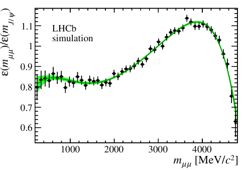
Figure 2: Efficiency to reconstruct, trigger and select simulated ${{{B}^{+}}}\!\rightarrow{{K}^{+}}{\mu^{+}}{\mu^{-}}$ decays as a function of the true dimuon mass. The efficiency is normalised to the efficiency at the ${J\mskip-3.0mu/\mskip-2.0mu\psi\mskip 2.0mu}$ meson mass. The band indicates the efficiency parameterisation used in this analysis and its statistical uncertainty.

Table 2: Parameters describing the efficiency to trigger, reconstruct and select simulated ${{{B}^{+}}}\!\rightarrow{{K}^{+}}{\mu^{+}\mu^{-}}$ decays as a function of $m_{\mu\mu}$.

	$\varepsilon_{0}$	$\varepsilon_{1}$	$\varepsilon_{2}$	$\varepsilon_{3}$	$\varepsilon_{4}$	$\varepsilon_{5}$	$\varepsilon_{6}$
Value	$\phantom{+}0.9262$	$\phantom{+}0.1279$	$-0.0532$	$-0.1857$	$-0.1269$	$-0.0205$	$-0.0229$
Uncertainty	$\phantom{+}0.0036$	$\phantom{+}0.0080$	$\phantom{+}0.0116$	$\phantom{+}0.0131$	$\phantom{+}0.0155$	$\phantom{+}0.0138$	$\phantom{+}0.0148$
Correlation	$\varepsilon_{0}$	$\varepsilon_{1}$	$\varepsilon_{2}$	$\varepsilon_{3}$	$\varepsilon_{4}$	$\varepsilon_{5}$	$\varepsilon_{6}$
$\varepsilon_{0}$	$\phantom{+}1.000$	$-0.340$	$\phantom{+}0.605$	$-0.208$	$\phantom{+}0.432$	$-$0.132	$\phantom{+}0.298$
$\varepsilon_{1}$		$\phantom{+}1.000$	$-0.345$	$\phantom{+}0.635$	$-0.207$	$\phantom{+}0.411$	$-0.094$
$\varepsilon_{2}$			+1.000	$-0.352$	$\phantom{+}0.684$	$-0.224$	$\phantom{+}0.455$
$\varepsilon_{3}$				$\phantom{+}1.000$	$-0.344$	$\phantom{+}0.608$	$-0.154$
$\varepsilon_{4}$					$\phantom{+}1.000$	$-0.344$	$\phantom{+}0.619$
$\varepsilon_{5}$						$\phantom{+}1.000$	$-0.259$
$\varepsilon_{6}$							$\phantom{+}1.000$

5.4 Background model

The reconstructed dimuon mass distribution of the combinatorial background candidates is taken from the $m_{K\mu\mu}$ upper mass sideband, $5620<m_{K\mu\mu}<5700{\mathrm{\,Me\kern-1.00006ptV\!/}c^{2}}$. When evaluating $m^{\rm rec}_{\mu\mu}$, $m_{K\mu\mu}$ is constrained to the centre of the sideband rather than to the known ${{B}^{+}}$ mass. Combinatorial background comprising a genuine ${J\mskip-3.0mu/\mskip-2.0mu\psi\mskip 2.0mu}$ or $\psi{(2S)}$ meson is described by the sum of two Gaussian functions. After applying the mass constraint, the means of the Gaussians do not correspond exactly to the known ${J\mskip-3.0mu/\mskip-2.0mu\psi\mskip 2.0mu}$ and $\psi{(2S)}$ masses. Combinatorial background comprising a dimuon pair that does not originate from a ${J\mskip-3.0mu/\mskip-2.0mu\psi\mskip 2.0mu}$ or $\psi{(2S)}$ meson is described by an ARGUS function [55]. The lineshape of the background from ${{{B}^{+}}}\!\rightarrow{{\pi}^{+}}{\mu^{+}\mu^{-}}$ decays, where the pion is mistakenly identified as a kaon, is taken from simulated events.

6 Results

The dimuon mass distributions and the projections of the fit to the data are shown in Fig. 3. Four solutions are obtained with almost equal likelihood values, which correspond to ambiguities in the signs of the ${J\mskip-3.0mu/\mskip-2.0mu\psi\mskip 2.0mu}$ and $\psi{(2S)}$ phases. The values of the phases and branching fractions of the vector meson resonances are listed in Table 3. The posterior values for the $f_{+}$ form factor are reported in Table 4. A $\chi^{2}$ test between the data and the model, with the binning scheme used in Fig. 3, results in a $\chi^{2}$ of 110 with 78 degrees of freedom. The largest disagreements between the data and the model are localised in the $m_{\mu\mu}$ region close to the ${J\mskip-3.0mu/\mskip-2.0mu\psi\mskip 2.0mu}$ pole mass and around 1.8${\mathrm{\,Ge\kern-1.00006ptV\!/}c^{2}}$. The latter is discussed in Sec. 7.

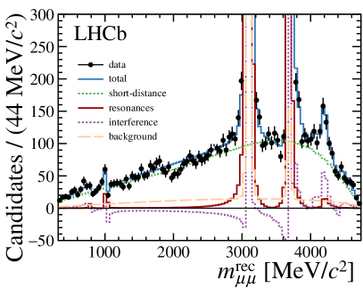
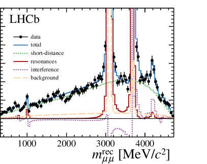
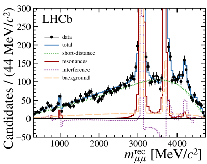
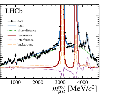
Figure 3: Fits to the dimuon mass distribution for the four different phase combinations that describe the data equally well. The plots show cases where the ${J\mskip-3.0mu/\mskip-2.0mu\psi\mskip 2.0mu}$ and $\psi{(2S)}$ phases are both negative (top left); the ${J\mskip-3.0mu/\mskip-2.0mu\psi\mskip 2.0mu}$ phase is positive and the $\psi{(2S)}$ phase is negative (top right); the ${J\mskip-3.0mu/\mskip-2.0mu\psi\mskip 2.0mu}$ phase is negative and the $\psi{(2S)}$ phase is positive (bottom left); and both phases are positive (bottom right). The component labelled interference refers to the interference between the short- and long-distance contributions to the decay. The $\chi^{2}$ value of the four solutions is almost identical, with a value of 110 for 78 degrees of freedom.

Table 3: Branching fractions and phases for each resonance in the fit for the four solutions of the ${J\mskip-3.0mu/\mskip-2.0mu\psi\mskip 2.0mu}$ and $\psi{(2S)}$ phases. Both statistical and systematic contributions are included in the uncertainties. There is a common systematic uncertainty of 4.5%, dominated by the uncertainty on the ${{{B}^{+}}}\rightarrow{{J\mskip-3.0mu/\mskip-2.0mu\psi\mskip 2.0mu}}{{K}^{+}}$ branching fraction, which provides the normalisation for all measurements.

	${J\mskip-3.0mu/\mskip-2.0mu\psi\mskip 2.0mu}$ negative/$\psi{(2S)}$ negative		${J\mskip-3.0mu/\mskip-2.0mu\psi\mskip 2.0mu}$ negative/$\psi{(2S)}$ positive
Resonance	Phase [rad]	Branching fraction	Phase [rad]	Branching fraction
$\rho(770)$	$-0.35\pm 0.54$	$(1.71\pm 0.25)\times 10^{-10}$	$-0.30\pm 0.54$	$(1.71\pm 0.25)\times 10^{-10}$
$\omega(782)$	$\phantom{+}0.26\pm 0.39$	$(4.93\pm 0.59)\times 10^{-10}$	$\phantom{+}0.30\pm 0.38$	$(4.93\pm 0.58)\times 10^{-10}$
$\phi(1020)$	$\phantom{+}0.47\pm 0.39$	$(2.53\pm 0.26)\times 10^{-9\phantom{0}}$	$\phantom{+}0.51\pm 0.37$	$(2.53\pm 0.26)\times 10^{-9\phantom{0}}$
$J/\psi$	$-1.66\pm 0.05$	–	$-1.50\pm 0.05$	–
$\psi(2S)$	$-1.93\pm 0.10$	$(4.64\pm 0.20)\times 10^{-6\phantom{0}}$	$\phantom{+}2.08\pm 0.11$	$(4.69\pm 0.20)\times 10^{-6\phantom{0}}$
$\psi(3770)$	$-2.13\pm 0.42$	$(1.38\pm 0.54)\times 10^{-9\phantom{0}}$	$-2.89\pm 0.19$	$(1.67\pm 0.61)\times 10^{-9\phantom{0}}$
$\psi(4040)$	$-2.52\pm 0.66$	$(4.17\pm 2.72)\times 10^{-10}$	$-2.69\pm 0.52$	$(4.25\pm 2.83)\times 10^{-10}$
$\psi(4160)$	$-1.90\pm 0.64$	$(2.61\pm 0.84)\times 10^{-9\phantom{0}}$	$-2.13\pm 0.33$	$(2.67\pm 0.85)\times 10^{-9\phantom{0}}$
$\psi(4415)$	$-2.52\pm 0.36$	$(6.04\pm 3.93)\times 10^{-10}$	$-2.43\pm 0.43$	$(7.10\pm 4.48)\times 10^{-10}$
	${J\mskip-3.0mu/\mskip-2.0mu\psi\mskip 2.0mu}$ positive/$\psi{(2S)}$ negative		${J\mskip-3.0mu/\mskip-2.0mu\psi\mskip 2.0mu}$ positive/$\psi{(2S)}$ positive
Resonance	Phase [rad]	Branching fraction	Phase [rad]	Branching fraction
$\rho(770)$	$-0.26\pm 0.54$	$(1.71\pm 0.25)\times 10^{-10}$	$-0.22\pm 0.54$	$(1.71\pm 0.25)\times 10^{-10}$
$\omega(782)$	$\phantom{+}0.35\pm 0.39$	$(4.93\pm 0.58)\times 10^{-10}$	$\phantom{+}0.38\pm 0.38$	$(4.93\pm 0.58)\times 10^{-10}$
$\phi(1020)$	$\phantom{+}0.58\pm 0.38$	$(2.53\pm 0.26)\times 10^{-9\phantom{0}}$	$\phantom{+}0.62\pm 0.37$	$(2.52\pm 0.26)\times 10^{-9\phantom{0}}$
$J/\psi$	$\phantom{+}1.47\pm 0.05$	–	$\phantom{+}1.63\pm 0.05$	–
$\psi(2S)$	$-2.21\pm 0.11$	$(4.63\pm 0.20)\times 10^{-6\phantom{0}}$	$\phantom{+}1.80\pm 0.10$	$(4.68\pm 0.20)\times 10^{-6\phantom{0}}$
$\psi(3770)$	$-2.40\pm 0.39$	$(1.39\pm 0.54)\times 10^{-9\phantom{0}}$	$-2.95\pm 0.14$	$(1.68\pm 0.61)\times 10^{-9\phantom{0}}$
$\psi(4040)$	$-2.64\pm 0.50$	$(4.05\pm 2.76)\times 10^{-10}$	$-2.75\pm 0.48$	$(4.30\pm 2.86)\times 10^{-10}$
$\psi(4160)$	$-2.11\pm 0.38$	$(2.62\pm 0.82)\times 10^{-9\phantom{0}}$	$-2.28\pm 0.24$	$(2.68\pm 0.81)\times 10^{-9\phantom{0}}$
$\psi(4415)$	$-2.42\pm 0.46$	$(6.13\pm 3.98)\times 10^{-10}$	$-2.31\pm 0.48$	$(7.12\pm 4.94)\times 10^{-10}$

Table 4: Coefficients of the form factor $f_{+}({q^{2}})$ as introduced in Eq. 8 with both prior (from Ref. [42]) and posterior values shown.

Coefficient	Ref. [42]	Fit result
$b^{+}_{0}$	$\phantom{+}0.466\pm 0.014$	$\phantom{+}0.465\pm 0.013$
$b^{+}_{1}$	$-0.89\pm 0.13$	$-0.81\pm 0.05$
$b^{+}_{2}$	$-0.21\pm 0.55$	$\phantom{+}0.03\pm 0.32$

The branching fraction of the short-distance component of the ${{{B}^{+}}}\!\rightarrow{{K}^{+}}{\mu^{+}}{\mu^{-}}$ decay can be calculated by integrating Eq. 1 after setting the amplitudes of the resonances to zero. This gives

$$\mathcal{B}({{{B}^{+}}}\!\rightarrow{{K}^{+}}{\mu^{+}}{\mu^{-}})=(4.37\pm 0.15\mathrm{\,(stat)}\pm 0.23\mathrm{\,(syst)})\times 10^{-7}\;,$$

where the statistical uncertainty includes the uncertainty on the form-factor predictions. The systematic uncertainty on the branching fraction is discussed in Sec. 7. This measurement is compatible with the branching fraction reported in Ref. [22]. The two results are based on the same data and therefore should not be used together in global fits. The branching fraction reported in Ref. [22] is based on a binned measurement in $q^{2}$ regions away from the narrow resonances ($\phi$, ${J\mskip-3.0mu/\mskip-2.0mu\psi\mskip 2.0mu}$ and $\psi{(2S)}$) and then extrapolated to the full $q^{2}$ range. The contribution from the broad resonances was thus included in that result.

A two-dimensional likelihood profile of $\mathcal{C}_{9}$ and $\mathcal{C}_{10}$ is also obtained as shown in Fig. 4. The intervals correspond to $\chi^{2}$ probabilities assuming two degrees of freedom. Only the quadrant with $\mathcal{C}_{9}$ and $\mathcal{C}_{10}$ values around the SM prediction is shown. The other quadrants can be obtained by mirroring in the axes. The branching fraction of the short-distance component provides a good constraint on the sum of $|\mathcal{C}_{9}|^{2}$ and $|\mathcal{C}_{10}|^{2}$ (see Eq. 1). This gives rise to the annular shape in the likelihood profile in Fig. 4. In addition, there is a modest ability for the fit to differentiate between $\mathcal{C}_{9}$ and $\mathcal{C}_{10}$ through the interference of the $\mathcal{C}_{9}$ component with the resonances. The visible interference pattern excludes very small values of $|\mathcal{C}_{9}|$. Overall, the correlation between $\mathcal{C}_{9}$ and $\mathcal{C}_{10}$ is approximately 90%. The best-fit point for the Wilson coefficients (in a given quadrant of the $\mathcal{C}_{9}$ and $\mathcal{C}_{10}$ plane) and the corresponding ${{{B}^{+}}}\!\rightarrow{{K}^{+}}{\mu^{+}\mu^{-}}$ branching fraction are the same for the four combinations of the ${J\mskip-3.0mu/\mskip-2.0mu\psi\mskip 2.0mu}$ and $\psi{(2S)}$ phases. Including statistical and systematic uncertainties, the fit results deviate from the SM prediction at the level of 3.0 standard deviations. The uncertainty is dominated by the precision of the form factors. The best-fit point prefers a value of $|\mathcal{C}_{10}|$ that is smaller than $|\mathcal{C}_{10}^{\rm SM}|$ and a value of $|\mathcal{C}_{9}|$ that is larger than $|\mathcal{C}_{9}^{\rm SM}|$. However, if $\mathcal{C}_{10}$ is fixed to its SM value, the fit prefers $|\mathcal{C}_{9}|<|\mathcal{C}_{9}^{\rm SM}|$. This is consistent with the results of global fits to $b\!\rightarrow s\ell^{+}\ell^{-}$ processes. Given the model assumptions in this paper, the interference with the ${J\mskip-3.0mu/\mskip-2.0mu\psi\mskip 2.0mu}$ meson is not able to explain the low value of the branching fraction of the ${{{B}^{+}}}\!\rightarrow{{K}^{+}}{\mu^{+}\mu^{-}}$ decay while keeping the values of $\mathcal{C}_{9}$ and $\mathcal{C}_{10}$ at their SM predictions.

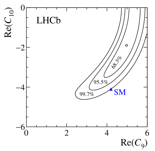
Figure 4: Two-dimensional likelihood profile for the Wilson coefficients $\mathcal{C}_{9}$ and $\mathcal{C}_{10}$. The SM point is indicated by the blue marker. The intervals correspond to $\chi^{2}$ probabilities with two degrees of freedom.

7 Systematic uncertainties

Sources of systematic uncertainty are considered separately for the phase and branching fraction measurements. In both cases, the largest systematic uncertainties are accounted for in the statistical uncertainty as they are included as nuisance parameters in the fit. For smaller sources of uncertainty, the fit is repeated with variations of the inputs and the difference is assigned as a systematic uncertainty. A summary of the remaining systematic uncertainties can be found in Table 5.

Table 5: Summary of systematic uncertainties. The branching fraction refers to the short-distance SM contribution. A dash indicates that the uncertainty is negligible.

Source	${J\mskip-3.0mu/\mskip-2.0mu\psi\mskip 2.0mu}$ phase	$\psi{(2S)}$ phase	Branching fraction	$\mathcal{C}_{9,10}$
Broad components	20$\mathrm{\,mrad}$	10$\mathrm{\,mrad}$	1.0%	0.05
Background model	10$\mathrm{\,mrad}$	10$\mathrm{\,mrad}$	1.0%	0.05
Efficiency model	03$\mathrm{\,mrad}$	10$\mathrm{\,mrad}$	1.0%	0.05
${\mathcal{B}}({{{B}^{+}}}\!\rightarrow{{J\mskip-3.0mu/\mskip-2.0mu\psi\mskip 2.0mu}}{{K}^{+}})$	—	—	4.2%	0.19

The parameters governing the behaviour of the tails of the resolution function are particularly correlated with the phases. The systematic uncertainty on the resolution model is included in the statistical uncertainty by allowing the resolution parameter values to vary in the fit. If the tail parameters are fixed to their central values, the statistical uncertainties on the phase measurements decrease by approximately 20%. The choice of parameterisation for the resolution model is validated using a large sample of simulated events and no additional uncertainty is assigned for the choice of model. For the branching fraction measurement, the uncertainty arising from the resolution model is negligible compared to other sources of systematic uncertainty.

Similarly to the resolution model, the systematic uncertainty associated with the knowledge of the $f_{+}({q^{2}})$ form factor is included in the statistical uncertainty. If the form-factor parameters are fixed to their best-fit values, the statistical uncertainties on the phases decrease by 4% (1%) for the ${J\mskip-3.0mu/\mskip-2.0mu\psi\mskip 2.0mu}$ ($\psi{(2S)}$) measurements. For the branching fraction, the uncertainty is 2%, which is of similar size as the statistical uncertainty.

At around $m_{\mu\mu}=1.8$${\mathrm{\,Ge\kern-1.00006ptV\!/}c^{2}}$ there is a small discrepancy between the data and the model (see Fig. 3). This is interpreted as a possible contribution from excited $\rho$, $\omega$ or $\phi$ resonances. Given the limited knowledge of the masses and widths of the states in this region, these broad states are neglected in the nominal fit. They are, however, visible in ${e^{+}e^{-}}\rightarrow\rm hadrons$ vacuum polarisation data [41]. To test the effect of such states on the phases of the ${J\mskip-3.0mu/\mskip-2.0mu\psi\mskip 2.0mu}$ and $\psi{(2S)}$ mesons, an additional relativistic Breit–Wigner amplitude is included with a width and mass that are allowed to vary in the fit. The inclusion of this Breit–Wigner amplitude marginally improves the fit quality around $m_{\mu\mu}=1.8$${\mathrm{\,Ge\kern-1.00006ptV\!/}c^{2}}$ and changes the ${J\mskip-3.0mu/\mskip-2.0mu\psi\mskip 2.0mu}$ ($\psi{(2S)}$) phase by 40% (20%) of its statistical uncertainty, which is added as a systematic effect. The magnitude of the amplitude is not statistically significant and its mean and width do not correspond to a known state. The phases of the other resonances in the fit have larger statistical uncertainties and the inclusion of this additional amplitude has a negligible effect on their fit values. Given that the contribution of this amplitude is small compared to the short-distance component, its effect on the branching fraction is only around 1%.

Other, smaller systematic uncertainties include modelling of the combinatorial background, calculation of the efficiency as a function of $q^{2}$ and the uncertainty on the ${{{B}^{+}}}\!\rightarrow{{J\mskip-3.0mu/\mskip-2.0mu\psi\mskip 2.0mu}}{{K}^{+}}$ branching fraction. The latter affects the branching fraction measurement and is obtained from Ref. [52], which results in a $4\%$ uncertainty.

8 Conclusions

This paper presents the first measurement of the phase difference between the short- and long-distance contributions to the ${{B}^{+}}\!\rightarrow{{K}^{+}}{\mu^{+}\mu^{-}}$ decay. The measurement is performed using a binned maximum likelihood fit to the dimuon mass distribution of the decays. The long-distance contributions are modelled as the sum of relativistic Breit–Wigner amplitudes representing different vector meson resonances decaying to muon pairs, each with their own magnitude and phase. The short-distance contribution is expressed in terms of an effective field theory description of the decay with the Wilson coefficients $\mathcal{C}_{9}$ and $\mathcal{C}_{10}$, which are taken to be real. These are left free in the fit and all other components set to their corresponding SM values. The $B\rightarrow K$ hadronic form factors are constrained in the fit to the predictions from Ref. [42].

The fit results in four approximately degenerate solutions corresponding to ambiguities in the signs of the ${J\mskip-3.0mu/\mskip-2.0mu\psi\mskip 2.0mu}$ and $\psi{(2S)}$ phases. The values of the ${J\mskip-3.0mu/\mskip-2.0mu\psi\mskip 2.0mu}$ phases are compatible with $\pm\tfrac{\pi}{2}$, which means that the interference with the short-distance component in dimuon mass regions far from their pole masses is small. The negative solution of the ${J\mskip-3.0mu/\mskip-2.0mu\psi\mskip 2.0mu}$ phase agrees qualitatively with the prediction of Ref. [47], where long-distance contributions are calculated at negative $q^{2}$ and extrapolated to the $q^{2}$ region below the ${J\mskip-3.0mu/\mskip-2.0mu\psi\mskip 2.0mu}$ pole-mass using a hadronic dispersion relation. The fit model, which includes the conventional $J^{PC}=1^{--}$ $c\bar{c}$ resonances, is found to describe the data well, with no significant evidence for the decays ${{{B}^{+}}}\!\rightarrow\psi(4040){{K}^{+}}$ or ${{{B}^{+}}}\!\rightarrow\psi(4415){{K}^{+}}$. The values of the $\psi(3770)$ and $\psi(4160)$ phases are compatible with those reported in Ref. [13].

The measurement of the Wilson coefficients prefers a value of $|\mathcal{C}_{10}|<|\mathcal{C}_{10}^{\rm SM}|$ and a value of $|\mathcal{C}_{9}|>|\mathcal{C}_{9}^{\rm SM}|$. If the value of $\mathcal{C}_{10}$ is set to that of $\mathcal{C}_{10}^{\rm SM}$, the measurement favours the region $|\mathcal{C}_{9}|<|\mathcal{C}_{9}^{\rm SM}|$. These results are similar to those reported previously in global analyses. The interference between the short- and long-distance contributions in the regions around the $\rho$, $\omega$ and the $\phi$, and in the region ${q^{2}}>m_{{\psi{(2S)}}}^{2}$, results in the exclusion of the hypothesis that $\mathcal{C}_{9}=0$ at more than 5 standard deviations. The dominant uncertainty on the measurements of $\mathcal{C}_{9}$ and $\mathcal{C}_{10}$ arises from the knowledge of the $B\rightarrow K$ hadronic form factors. The current data set allows the uncertainties on these hadronic parameters to be reduced. Improved inputs on the form factors from lattice QCD calculations and the larger data set that will be available at the end of the LHC Run 2 are needed to further improve the measurement of the Wilson coefficients.

A similar strategy to the one applied in this paper can be extended to other $b\rightarrow s\ell^{+}\ell^{-}$ decay processes to understand the influence of hadronic resonances on global fits for $\mathcal{C}_{9}$ and $\mathcal{C}_{10}$. However, the situation is more complicated in decays where the strange hadron is not a pseudoscalar meson as the amplitudes corresponding to different helicity states of the hadron can have different relative phases.

Finally, a measurement of the branching fraction of the short-distance component of ${{B}^{+}}\!\rightarrow{{K}^{+}}{\mu^{+}\mu^{-}}$ decays is also reported and is found to be

$$\mathcal{B}({{{B}^{+}}}\!\rightarrow{{K}^{+}}{\mu^{+}}{\mu^{-}})=(4.37\pm 0.15\mathrm{\,(stat)}\pm 0.23\mathrm{\,(syst)})\times 10^{-7}\;,$$

where the first uncertainty is statistical and second is systematic. In contrast to previous analyses, the measurement is performed across the full $q^{2}$ region accounting for the interference with the long-distance contributions and without any veto of resonance-dominated regions of the phase space. The value of the branching fraction is found to be compatible with previous measurements [22], but smaller than the SM prediction [42].

LHCb collaboration

R. Aaij⁴⁰, B. Adeva³⁹, M. Adinolfi⁴⁸, Z. Ajaltouni⁵, S. Akar⁵⁹, J. Albrecht¹⁰, F. Alessio⁴⁰, M. Alexander⁵³, S. Ali⁴³, G. Alkhazov³¹, P. Alvarez Cartelle⁵⁵, A.A. Alves Jr⁵⁹, S. Amato², S. Amerio²³, Y. Amhis⁷, L. An³, L. Anderlini¹⁸, G. Andreassi⁴¹, M. Andreotti^17,g, J.E. Andrews⁶⁰, R.B. Appleby⁵⁶, F. Archilli⁴³, P. d’Argent¹², J. Arnau Romeu⁶, A. Artamonov³⁷, M. Artuso⁶¹, E. Aslanides⁶, G. Auriemma²⁶, M. Baalouch⁵, I. Babuschkin⁵⁶, S. Bachmann¹², J.J. Back⁵⁰, A. Badalov³⁸, C. Baesso⁶², S. Baker⁵⁵, V. Balagura^7,c, W. Baldini¹⁷, R.J. Barlow⁵⁶, C. Barschel⁴⁰, S. Barsuk⁷, W. Barter⁴⁰, M. Baszczyk²⁷, V. Batozskaya²⁹, B. Batsukh⁶¹, V. Battista⁴¹, A. Bay⁴¹, L. Beaucourt⁴, J. Beddow⁵³, F. Bedeschi²⁴, I. Bediaga¹, L.J. Bel⁴³, V. Bellee⁴¹, N. Belloli^21,i, K. Belous³⁷, I. Belyaev³², E. Ben-Haim⁸, G. Bencivenni¹⁹, S. Benson⁴³, A. Berezhnoy³³, R. Bernet⁴², A. Bertolin²³, C. Betancourt⁴², F. Betti¹⁵, M.-O. Bettler⁴⁰, M. van Beuzekom⁴³, Ia. Bezshyiko⁴², S. Bifani⁴⁷, P. Billoir⁸, T. Bird⁵⁶, A. Birnkraut¹⁰, A. Bitadze⁵⁶, A. Bizzeti^18,u, T. Blake⁵⁰, F. Blanc⁴¹, J. Blouw^11,†, S. Blusk⁶¹, V. Bocci²⁶, T. Boettcher⁵⁸, A. Bondar^36,w, N. Bondar^31,40, W. Bonivento¹⁶, I. Bordyuzhin³², A. Borgheresi^21,i, S. Borghi⁵⁶, M. Borisyak³⁵, M. Borsato³⁹, F. Bossu⁷, M. Boubdir⁹, T.J.V. Bowcock⁵⁴, E. Bowen⁴², C. Bozzi^17,40, S. Braun¹², M. Britsch¹², T. Britton⁶¹, J. Brodzicka⁵⁶, E. Buchanan⁴⁸, C. Burr⁵⁶, A. Bursche², J. Buytaert⁴⁰, S. Cadeddu¹⁶, R. Calabrese^17,g, M. Calvi^21,i, M. Calvo Gomez^38,m, A. Camboni³⁸, P. Campana¹⁹, D.H. Campora Perez⁴⁰, L. Capriotti⁵⁶, A. Carbone^15,e, G. Carboni^25,j, R. Cardinale^20,h, A. Cardini¹⁶, P. Carniti^21,i, L. Carson⁵², K. Carvalho Akiba², G. Casse⁵⁴, L. Cassina^21,i, L. Castillo Garcia⁴¹, M. Cattaneo⁴⁰, G. Cavallero²⁰, R. Cenci^24,t, D. Chamont⁷, M. Charles⁸, Ph. Charpentier⁴⁰, G. Chatzikonstantinidis⁴⁷, M. Chefdeville⁴, S. Chen⁵⁶, S.-F. Cheung⁵⁷, V. Chobanova³⁹, M. Chrzaszcz^42,27, X. Cid Vidal³⁹, G. Ciezarek⁴³, P.E.L. Clarke⁵², M. Clemencic⁴⁰, H.V. Cliff⁴⁹, J. Closier⁴⁰, V. Coco⁵⁹, J. Cogan⁶, E. Cogneras⁵, V. Cogoni^16,40,f, L. Cojocariu³⁰, G. Collazuol^23,o, P. Collins⁴⁰, A. Comerma-Montells¹², A. Contu⁴⁰, A. Cook⁴⁸, G. Coombs⁴⁰, S. Coquereau³⁸, G. Corti⁴⁰, M. Corvo^17,g, C.M. Costa Sobral⁵⁰, B. Couturier⁴⁰, G.A. Cowan⁵², D.C. Craik⁵², A. Crocombe⁵⁰, M. Cruz Torres⁶², S. Cunliffe⁵⁵, R. Currie⁵⁵, C. D’Ambrosio⁴⁰, F. Da Cunha Marinho², E. Dall’Occo⁴³, J. Dalseno⁴⁸, P.N.Y. David⁴³, A. Davis³, K. De Bruyn⁶, S. De Capua⁵⁶, M. De Cian¹², J.M. De Miranda¹, L. De Paula², M. De Serio^14,d, P. De Simone¹⁹, C.-T. Dean⁵³, D. Decamp⁴, M. Deckenhoff¹⁰, L. Del Buono⁸, M. Demmer¹⁰, A. Dendek²⁸, D. Derkach³⁵, O. Deschamps⁵, F. Dettori⁴⁰, B. Dey²², A. Di Canto⁴⁰, H. Dijkstra⁴⁰, F. Dordei⁴⁰, M. Dorigo⁴¹, A. Dosil Suárez³⁹, A. Dovbnya⁴⁵, K. Dreimanis⁵⁴, L. Dufour⁴³, G. Dujany⁵⁶, K. Dungs⁴⁰, P. Durante⁴⁰, R. Dzhelyadin³⁷, A. Dziurda⁴⁰, A. Dzyuba³¹, N. Déléage⁴, S. Easo⁵¹, M. Ebert⁵², U. Egede⁵⁵, V. Egorychev³², S. Eidelman^36,w, S. Eisenhardt⁵², U. Eitschberger¹⁰, R. Ekelhof¹⁰, L. Eklund⁵³, S. Ely⁶¹, S. Esen¹², H.M. Evans⁴⁹, T. Evans⁵⁷, A. Falabella¹⁵, N. Farley⁴⁷, S. Farry⁵⁴, R. Fay⁵⁴, D. Fazzini^21,i, D. Ferguson⁵², A. Fernandez Prieto³⁹, F. Ferrari^15,40, F. Ferreira Rodrigues², M. Ferro-Luzzi⁴⁰, S. Filippov³⁴, R.A. Fini¹⁴, M. Fiore^17,g, M. Fiorini^17,g, M. Firlej²⁸, C. Fitzpatrick⁴¹, T. Fiutowski²⁸, F. Fleuret^7,b, K. Fohl⁴⁰, M. Fontana^16,40, F. Fontanelli^20,h, D.C. Forshaw⁶¹, R. Forty⁴⁰, V. Franco Lima⁵⁴, M. Frank⁴⁰, C. Frei⁴⁰, J. Fu^22,q, W. Funk⁴⁰, E. Furfaro^25,j, C. Färber⁴⁰, A. Gallas Torreira³⁹, D. Galli^15,e, S. Gallorini²³, S. Gambetta⁵², M. Gandelman², P. Gandini⁵⁷, Y. Gao³, L.M. Garcia Martin⁶⁹, J. García Pardiñas³⁹, J. Garra Tico⁴⁹, L. Garrido³⁸, P.J. Garsed⁴⁹, D. Gascon³⁸, C. Gaspar⁴⁰, L. Gavardi¹⁰, G. Gazzoni⁵, D. Gerick¹², E. Gersabeck¹², M. Gersabeck⁵⁶, T. Gershon⁵⁰, Ph. Ghez⁴, S. Gianì⁴¹, V. Gibson⁴⁹, O.G. Girard⁴¹, L. Giubega³⁰, K. Gizdov⁵², V.V. Gligorov⁸, D. Golubkov³², A. Golutvin^55,40, A. Gomes^1,a, I.V. Gorelov³³, C. Gotti^21,i, R. Graciani Diaz³⁸, L.A. Granado Cardoso⁴⁰, E. Graugés³⁸, E. Graverini⁴², G. Graziani¹⁸, A. Grecu³⁰, P. Griffith⁴⁷, L. Grillo^21,40,i, B.R. Gruberg Cazon⁵⁷, O. Grünberg⁶⁷, E. Gushchin³⁴, Yu. Guz³⁷, T. Gys⁴⁰, C. Göbel⁶², T. Hadavizadeh⁵⁷, C. Hadjivasiliou⁵, G. Haefeli⁴¹, C. Haen⁴⁰, S.C. Haines⁴⁹, S. Hall⁵⁵, B. Hamilton⁶⁰, X. Han¹², S. Hansmann-Menzemer¹², N. Harnew⁵⁷, S.T. Harnew⁴⁸, J. Harrison⁵⁶, M. Hatch⁴⁰, J. He⁶³, T. Head⁴¹, A. Heister⁹, K. Hennessy⁵⁴, P. Henrard⁵, L. Henry⁸, E. van Herwijnen⁴⁰, M. Heß⁶⁷, A. Hicheur², D. Hill⁵⁷, C. Hombach⁵⁶, H. Hopchev⁴¹, W. Hulsbergen⁴³, T. Humair⁵⁵, M. Hushchyn³⁵, D. Hutchcroft⁵⁴, M. Idzik²⁸, P. Ilten⁵⁸, R. Jacobsson⁴⁰, A. Jaeger¹², J. Jalocha⁵⁷, E. Jans⁴³, A. Jawahery⁶⁰, F. Jiang³, M. John⁵⁷, D. Johnson⁴⁰, C.R. Jones⁴⁹, C. Joram⁴⁰, B. Jost⁴⁰, N. Jurik⁵⁷, S. Kandybei⁴⁵, M. Karacson⁴⁰, J.M. Kariuki⁴⁸, S. Karodia⁵³, M. Kecke¹², M. Kelsey⁶¹, M. Kenzie⁴⁹, T. Ketel⁴⁴, E. Khairullin³⁵, B. Khanji¹², C. Khurewathanakul⁴¹, T. Kirn⁹, S. Klaver⁵⁶, K. Klimaszewski²⁹, S. Koliiev⁴⁶, M. Kolpin¹², I. Komarov⁴¹, R.F. Koopman⁴⁴, P. Koppenburg⁴³, A. Kosmyntseva³², A. Kozachuk³³, M. Kozeiha⁵, L. Kravchuk³⁴, K. Kreplin¹², M. Kreps⁵⁰, P. Krokovny^36,w, F. Kruse¹⁰, W. Krzemien²⁹, W. Kucewicz^27,l, M. Kucharczyk²⁷, V. Kudryavtsev^36,w, A.K. Kuonen⁴¹, K. Kurek²⁹, T. Kvaratskheliya^32,40, D. Lacarrere⁴⁰, G. Lafferty⁵⁶, A. Lai¹⁶, G. Lanfranchi¹⁹, C. Langenbruch⁹, T. Latham⁵⁰, C. Lazzeroni⁴⁷, R. Le Gac⁶, J. van Leerdam⁴³, A. Leflat^33,40, J. Lefrançois⁷, R. Lefèvre⁵, F. Lemaitre⁴⁰, E. Lemos Cid³⁹, O. Leroy⁶, T. Lesiak²⁷, B. Leverington¹², T. Li³, Y. Li⁷, T. Likhomanenko^35,68, R. Lindner⁴⁰, C. Linn⁴⁰, F. Lionetto⁴², X. Liu³, D. Loh⁵⁰, I. Longstaff⁵³, J.H. Lopes², D. Lucchesi^23,o, M. Lucio Martinez³⁹, H. Luo⁵², A. Lupato²³, E. Luppi^17,g, O. Lupton⁴⁰, A. Lusiani²⁴, X. Lyu⁶³, F. Machefert⁷, F. Maciuc³⁰, O. Maev³¹, K. Maguire⁵⁶, S. Malde⁵⁷, A. Malinin⁶⁸, T. Maltsev³⁶, G. Manca^16,f, G. Mancinelli⁶, P. Manning⁶¹, J. Maratas^5,v, J.F. Marchand⁴, U. Marconi¹⁵, C. Marin Benito³⁸, M. Marinangeli⁴¹, P. Marino^24,t, J. Marks¹², G. Martellotti²⁶, M. Martin⁶, M. Martinelli⁴¹, D. Martinez Santos³⁹, F. Martinez Vidal⁶⁹, D. Martins Tostes², L.M. Massacrier⁷, A. Massafferri¹, R. Matev⁴⁰, A. Mathad⁵⁰, Z. Mathe⁴⁰, C. Matteuzzi²¹, A. Mauri⁴², E. Maurice^7,b, B. Maurin⁴¹, A. Mazurov⁴⁷, M. McCann^55,40, A. McNab⁵⁶, R. McNulty¹³, B. Meadows⁵⁹, F. Meier¹⁰, M. Meissner¹², D. Melnychuk²⁹, M. Merk⁴³, A. Merli^22,q, E. Michielin²³, D.A. Milanes⁶⁶, M.-N. Minard⁴, D.S. Mitzel¹², A. Mogini⁸, J. Molina Rodriguez¹, I.A. Monroy⁶⁶, S. Monteil⁵, M. Morandin²³, P. Morawski²⁸, A. Mordà⁶, M.J. Morello^24,t, O. Morgunova⁶⁸, J. Moron²⁸, A.B. Morris⁵², R. Mountain⁶¹, F. Muheim⁵², M. Mulder⁴³, M. Mussini¹⁵, D. Müller⁵⁶, J. Müller¹⁰, K. Müller⁴², V. Müller¹⁰, P. Naik⁴⁸, T. Nakada⁴¹, R. Nandakumar⁵¹, A. Nandi⁵⁷, I. Nasteva², M. Needham⁵², N. Neri²², S. Neubert¹², N. Neufeld⁴⁰, M. Neuner¹², T.D. Nguyen⁴¹, C. Nguyen-Mau^41,n, S. Nieswand⁹, R. Niet¹⁰, N. Nikitin³³, T. Nikodem¹², A. Nogay⁶⁸, A. Novoselov³⁷, D.P. O’Hanlon⁵⁰, A. Oblakowska-Mucha²⁸, V. Obraztsov³⁷, S. Ogilvy¹⁹, R. Oldeman^16,f, C.J.G. Onderwater⁷⁰, J.M. Otalora Goicochea², A. Otto⁴⁰, P. Owen⁴², A. Oyanguren⁶⁹, P.R. Pais⁴¹, A. Palano^14,d, F. Palombo^22,q, M. Palutan¹⁹, A. Papanestis⁵¹, M. Pappagallo^14,d, L.L. Pappalardo^17,g, W. Parker⁶⁰, C. Parkes⁵⁶, G. Passaleva¹⁸, A. Pastore^14,d, G.D. Patel⁵⁴, M. Patel⁵⁵, C. Patrignani^15,e, A. Pearce⁴⁰, A. Pellegrino⁴³, G. Penso²⁶, M. Pepe Altarelli⁴⁰, S. Perazzini⁴⁰, P. Perret⁵, L. Pescatore⁴⁷, K. Petridis⁴⁸, A. Petrolini^20,h, A. Petrov⁶⁸, M. Petruzzo^22,q, E. Picatoste Olloqui³⁸, B. Pietrzyk⁴, M. Pikies²⁷, D. Pinci²⁶, A. Pistone²⁰, A. Piucci¹², V. Placinta³⁰, S. Playfer⁵², M. Plo Casasus³⁹, T. Poikela⁴⁰, F. Polci⁸, A. Poluektov^50,36, I. Polyakov⁶¹, E. Polycarpo², G.J. Pomery⁴⁸, A. Popov³⁷, D. Popov^11,40, B. Popovici³⁰, S. Poslavskii³⁷, C. Potterat², E. Price⁴⁸, J.D. Price⁵⁴, J. Prisciandaro^39,40, A. Pritchard⁵⁴, C. Prouve⁴⁸, V. Pugatch⁴⁶, A. Puig Navarro⁴², G. Punzi^24,p, W. Qian⁵⁰, R. Quagliani^7,48, B. Rachwal²⁷, J.H. Rademacker⁴⁸, M. Rama²⁴, M. Ramos Pernas³⁹, M.S. Rangel², I. Raniuk⁴⁵, F. Ratnikov³⁵, G. Raven⁴⁴, F. Redi⁵⁵, S. Reichert¹⁰, A.C. dos Reis¹, C. Remon Alepuz⁶⁹, V. Renaudin⁷, S. Ricciardi⁵¹, S. Richards⁴⁸, M. Rihl⁴⁰, K. Rinnert⁵⁴, V. Rives Molina³⁸, P. Robbe^7,40, A.B. Rodrigues¹, E. Rodrigues⁵⁹, J.A. Rodriguez Lopez⁶⁶, P. Rodriguez Perez^56,†, A. Rogozhnikov³⁵, S. Roiser⁴⁰, A. Rollings⁵⁷, V. Romanovskiy³⁷, A. Romero Vidal³⁹, J.W. Ronayne¹³, M. Rotondo¹⁹, M.S. Rudolph⁶¹, T. Ruf⁴⁰, P. Ruiz Valls⁶⁹, J.J. Saborido Silva³⁹, E. Sadykhov³², N. Sagidova³¹, B. Saitta^16,f, V. Salustino Guimaraes¹, C. Sanchez Mayordomo⁶⁹, B. Sanmartin Sedes³⁹, R. Santacesaria²⁶, C. Santamarina Rios³⁹, M. Santimaria¹⁹, E. Santovetti^25,j, A. Sarti^19,k, C. Satriano^26,s, A. Satta²⁵, D.M. Saunders⁴⁸, D. Savrina^32,33, S. Schael⁹, M. Schellenberg¹⁰, M. Schiller⁵³, H. Schindler⁴⁰, M. Schlupp¹⁰, M. Schmelling¹¹, T. Schmelzer¹⁰, B. Schmidt⁴⁰, O. Schneider⁴¹, A. Schopper⁴⁰, K. Schubert¹⁰, M. Schubiger⁴¹, M.-H. Schune⁷, R. Schwemmer⁴⁰, B. Sciascia¹⁹, A. Sciubba^26,k, A. Semennikov³², A. Sergi⁴⁷, N. Serra⁴², J. Serrano⁶, L. Sestini²³, P. Seyfert²¹, M. Shapkin³⁷, I. Shapoval⁴⁵, Y. Shcheglov³¹, T. Shears⁵⁴, L. Shekhtman^36,w, V. Shevchenko⁶⁸, B.G. Siddi^17,40, R. Silva Coutinho⁴², L. Silva de Oliveira², G. Simi^23,o, S. Simone^14,d, M. Sirendi⁴⁹, N. Skidmore⁴⁸, T. Skwarnicki⁶¹, E. Smith⁵⁵, I.T. Smith⁵², J. Smith⁴⁹, M. Smith⁵⁵, H. Snoek⁴³, l. Soares Lavra¹, M.D. Sokoloff⁵⁹, F.J.P. Soler⁵³, B. Souza De Paula², B. Spaan¹⁰, P. Spradlin⁵³, S. Sridharan⁴⁰, F. Stagni⁴⁰, M. Stahl¹², S. Stahl⁴⁰, P. Stefko⁴¹, S. Stefkova⁵⁵, O. Steinkamp⁴², S. Stemmle¹², O. Stenyakin³⁷, H. Stevens¹⁰, S. Stevenson⁵⁷, S. Stoica³⁰, S. Stone⁶¹, B. Storaci⁴², S. Stracka^24,p, M. Straticiuc³⁰, U. Straumann⁴², L. Sun⁶⁴, W. Sutcliffe⁵⁵, K. Swientek²⁸, V. Syropoulos⁴⁴, M. Szczekowski²⁹, T. Szumlak²⁸, S. T’Jampens⁴, A. Tayduganov⁶, T. Tekampe¹⁰, G. Tellarini^17,g, F. Teubert⁴⁰, E. Thomas⁴⁰, J. van Tilburg⁴³, M.J. Tilley⁵⁵, V. Tisserand⁴, M. Tobin⁴¹, S. Tolk⁴⁹, L. Tomassetti^17,g, D. Tonelli⁴⁰, S. Topp-Joergensen⁵⁷, F. Toriello⁶¹, E. Tournefier⁴, S. Tourneur⁴¹, K. Trabelsi⁴¹, M. Traill⁵³, M.T. Tran⁴¹, M. Tresch⁴², A. Trisovic⁴⁰, A. Tsaregorodtsev⁶, P. Tsopelas⁴³, A. Tully⁴⁹, N. Tuning⁴³, A. Ukleja²⁹, A. Ustyuzhanin³⁵, U. Uwer¹², C. Vacca^16,f, V. Vagnoni^15,40, A. Valassi⁴⁰, S. Valat⁴⁰, G. Valenti¹⁵, R. Vazquez Gomez¹⁹, P. Vazquez Regueiro³⁹, S. Vecchi¹⁷, M. van Veghel⁴³, J.J. Velthuis⁴⁸, M. Veltri^18,r, G. Veneziano⁵⁷, A. Venkateswaran⁶¹, M. Vernet⁵, M. Vesterinen¹², J.V. Viana Barbosa⁴⁰, B. Viaud⁷, D.  Vieira⁶³, M. Vieites Diaz³⁹, H. Viemann⁶⁷, X. Vilasis-Cardona^38,m, M. Vitti⁴⁹, V. Volkov³³, A. Vollhardt⁴², B. Voneki⁴⁰, A. Vorobyev³¹, V. Vorobyev^36,w, C. Voß⁹, J.A. de Vries⁴³, C. Vázquez Sierra³⁹, R. Waldi⁶⁷, C. Wallace⁵⁰, R. Wallace¹³, J. Walsh²⁴, J. Wang⁶¹, D.R. Ward⁴⁹, H.M. Wark⁵⁴, N.K. Watson⁴⁷, D. Websdale⁵⁵, A. Weiden⁴², M. Whitehead⁴⁰, J. Wicht⁵⁰, G. Wilkinson^57,40, M. Wilkinson⁶¹, M. Williams⁴⁰, M.P. Williams⁴⁷, M. Williams⁵⁸, T. Williams⁴⁷, F.F. Wilson⁵¹, J. Wimberley⁶⁰, J. Wishahi¹⁰, W. Wislicki²⁹, M. Witek²⁷, G. Wormser⁷, S.A. Wotton⁴⁹, K. Wraight⁵³, K. Wyllie⁴⁰, Y. Xie⁶⁵, Z. Xing⁶¹, Z. Xu⁴¹, Z. Yang³, Y. Yao⁶¹, H. Yin⁶⁵, J. Yu⁶⁵, X. Yuan^36,w, O. Yushchenko³⁷, K.A. Zarebski⁴⁷, M. Zavertyaev^11,c, L. Zhang³, Y. Zhang⁷, Y. Zhang⁶³, A. Zhelezov¹², Y. Zheng⁶³, X. Zhu³, V. Zhukov³³, S. Zucchelli¹⁵.

¹Centro Brasileiro de Pesquisas Físicas (CBPF), Rio de Janeiro, Brazil
²Universidade Federal do Rio de Janeiro (UFRJ), Rio de Janeiro, Brazil
³Center for High Energy Physics, Tsinghua University, Beijing, China
⁴LAPP, Université Savoie Mont-Blanc, CNRS/IN2P3, Annecy-Le-Vieux, France
⁵Clermont Université, Université Blaise Pascal, CNRS/IN2P3, LPC, Clermont-Ferrand, France
⁶CPPM, Aix-Marseille Université, CNRS/IN2P3, Marseille, France
⁷LAL, Université Paris-Sud, CNRS/IN2P3, Orsay, France
⁸LPNHE, Université Pierre et Marie Curie, Université Paris Diderot, CNRS/IN2P3, Paris, France
⁹I. Physikalisches Institut, RWTH Aachen University, Aachen, Germany
¹⁰Fakultät Physik, Technische Universität Dortmund, Dortmund, Germany
¹¹Max-Planck-Institut für Kernphysik (MPIK), Heidelberg, Germany
¹²Physikalisches Institut, Ruprecht-Karls-Universität Heidelberg, Heidelberg, Germany
¹³School of Physics, University College Dublin, Dublin, Ireland
¹⁴Sezione INFN di Bari, Bari, Italy
¹⁵Sezione INFN di Bologna, Bologna, Italy
¹⁶Sezione INFN di Cagliari, Cagliari, Italy
¹⁷Sezione INFN di Ferrara, Ferrara, Italy
¹⁸Sezione INFN di Firenze, Firenze, Italy
¹⁹Laboratori Nazionali dell’INFN di Frascati, Frascati, Italy
²⁰Sezione INFN di Genova, Genova, Italy
²¹Sezione INFN di Milano Bicocca, Milano, Italy
²²Sezione INFN di Milano, Milano, Italy
²³Sezione INFN di Padova, Padova, Italy
²⁴Sezione INFN di Pisa, Pisa, Italy
²⁵Sezione INFN di Roma Tor Vergata, Roma, Italy
²⁶Sezione INFN di Roma La Sapienza, Roma, Italy
²⁷Henryk Niewodniczanski Institute of Nuclear Physics Polish Academy of Sciences, Kraków, Poland
²⁸AGH - University of Science and Technology, Faculty of Physics and Applied Computer Science, Kraków, Poland
²⁹National Center for Nuclear Research (NCBJ), Warsaw, Poland
³⁰Horia Hulubei National Institute of Physics and Nuclear Engineering, Bucharest-Magurele, Romania
³¹Petersburg Nuclear Physics Institute (PNPI), Gatchina, Russia
³²Institute of Theoretical and Experimental Physics (ITEP), Moscow, Russia
³³Institute of Nuclear Physics, Moscow State University (SINP MSU), Moscow, Russia
³⁴Institute for Nuclear Research of the Russian Academy of Sciences (INR RAN), Moscow, Russia
³⁵Yandex School of Data Analysis, Moscow, Russia
³⁶Budker Institute of Nuclear Physics (SB RAS), Novosibirsk, Russia
³⁷Institute for High Energy Physics (IHEP), Protvino, Russia
³⁸ICCUB, Universitat de Barcelona, Barcelona, Spain
³⁹Universidad de Santiago de Compostela, Santiago de Compostela, Spain
⁴⁰European Organization for Nuclear Research (CERN), Geneva, Switzerland
⁴¹Institute of Physics, Ecole Polytechnique Fédérale de Lausanne (EPFL), Lausanne, Switzerland
⁴²Physik-Institut, Universität Zürich, Zürich, Switzerland
⁴³Nikhef National Institute for Subatomic Physics, Amsterdam, The Netherlands
⁴⁴Nikhef National Institute for Subatomic Physics and VU University Amsterdam, Amsterdam, The Netherlands
⁴⁵NSC Kharkiv Institute of Physics and Technology (NSC KIPT), Kharkiv, Ukraine
⁴⁶Institute for Nuclear Research of the National Academy of Sciences (KINR), Kyiv, Ukraine
⁴⁷University of Birmingham, Birmingham, United Kingdom
⁴⁸H.H. Wills Physics Laboratory, University of Bristol, Bristol, United Kingdom
⁴⁹Cavendish Laboratory, University of Cambridge, Cambridge, United Kingdom
⁵⁰Department of Physics, University of Warwick, Coventry, United Kingdom
⁵¹STFC Rutherford Appleton Laboratory, Didcot, United Kingdom
⁵²School of Physics and Astronomy, University of Edinburgh, Edinburgh, United Kingdom
⁵³School of Physics and Astronomy, University of Glasgow, Glasgow, United Kingdom
⁵⁴Oliver Lodge Laboratory, University of Liverpool, Liverpool, United Kingdom
⁵⁵Imperial College London, London, United Kingdom
⁵⁶School of Physics and Astronomy, University of Manchester, Manchester, United Kingdom
⁵⁷Department of Physics, University of Oxford, Oxford, United Kingdom
⁵⁸Massachusetts Institute of Technology, Cambridge, MA, United States
⁵⁹University of Cincinnati, Cincinnati, OH, United States
⁶⁰University of Maryland, College Park, MD, United States
⁶¹Syracuse University, Syracuse, NY, United States
⁶²Pontifícia Universidade Católica do Rio de Janeiro (PUC-Rio), Rio de Janeiro, Brazil, associated to ^2
63University of Chinese Academy of Sciences, Beijing, China, associated to ^3
64School of Physics and Technology, Wuhan University, Wuhan, China, associated to ^3
65Institute of Particle Physics, Central China Normal University, Wuhan, Hubei, China, associated to ^3
66Departamento de Fisica , Universidad Nacional de Colombia, Bogota, Colombia, associated to ^8
67Institut für Physik, Universität Rostock, Rostock, Germany, associated to ^12
68National Research Centre Kurchatov Institute, Moscow, Russia, associated to ^32
69Instituto de Fisica Corpuscular (IFIC), Universitat de Valencia-CSIC, Valencia, Spain, associated to ^38
70Van Swinderen Institute, University of Groningen, Groningen, The Netherlands, associated to <sup>43

a</sup>Universidade Federal do Triângulo Mineiro (UFTM), Uberaba-MG, Brazil
^bLaboratoire Leprince-Ringuet, Palaiseau, France
^cP.N. Lebedev Physical Institute, Russian Academy of Science (LPI RAS), Moscow, Russia
^dUniversità di Bari, Bari, Italy
^eUniversità di Bologna, Bologna, Italy
^fUniversità di Cagliari, Cagliari, Italy
^gUniversità di Ferrara, Ferrara, Italy
^hUniversità di Genova, Genova, Italy
ⁱUniversità di Milano Bicocca, Milano, Italy
^jUniversità di Roma Tor Vergata, Roma, Italy
^kUniversità di Roma La Sapienza, Roma, Italy
^lAGH - University of Science and Technology, Faculty of Computer Science, Electronics and Telecommunications, Kraków, Poland
^mLIFAELS, La Salle, Universitat Ramon Llull, Barcelona, Spain
ⁿHanoi University of Science, Hanoi, Viet Nam
^oUniversità di Padova, Padova, Italy
^pUniversità di Pisa, Pisa, Italy
^qUniversità degli Studi di Milano, Milano, Italy
^rUniversità di Urbino, Urbino, Italy
^sUniversità della Basilicata, Potenza, Italy
^tScuola Normale Superiore, Pisa, Italy
^uUniversità di Modena e Reggio Emilia, Modena, Italy
^vIligan Institute of Technology (IIT), Iligan, Philippines
^wNovosibirsk State University, Novosibirsk, Russia
^†Deceased

References

- [1] S. Descotes-Genon, J. Matias, and J. Virto, Understanding the anomaly, Phys. Rev. D88 (2013) 074002, arXiv:1307.5683
- [2] W. Altmannshofer and D. M. Straub, New physics in ?, Eur. Phys. J. C73 (2013) 2646, arXiv:1308.1501
- [3] W. Altmannshofer, S. Gori, M. Pospelov, and I. Yavin, Quark flavor transitions in models, Phys. Rev. D89 (2014) 095033, arXiv:1403.1269
- [4] F. Mahmoudi, S. Neshatpour, and J. Virto, optimised observables in the MSSM, Eur. Phys. J. C74 (2014) 2927, arXiv:1401.2145
- [5] A. Crivellin, G. D’Ambrosio, and J. Heeck, Explaining , and in a two-Higgs-doublet model with gauged , Phys. Rev. Lett. 114 (2015) 151801, arXiv:1501.00993
- [6] S. Descotes-Genon, L. Hofer, J. Matias, and J. Virto, Global analysis of anomalies, JHEP 06 (2016) 092, arXiv:1510.04239
- [7] T. Hurth, F. Mahmoudi, and S. Neshatpour, On the anomalies in the latest LHCb data, Nucl. Phys. B909 (2016) 737, arXiv:1603.00865
- [8] S. Jäger and J. Martin Camalich, On at small dilepton invariant mass, power corrections, and new physics, JHEP 05 (2013) 043, arXiv:1212.2263
- [9] F. Beaujean, C. Bobeth, and D. van Dyk, Comprehensive Bayesian analysis of rare (semi)leptonic and radiative decays, Eur. Phys. J. C74 (2014) 2897, arXiv:1310.2478
- [10] T. Hurth and F. Mahmoudi, On the LHCb anomaly in B , JHEP 04 (2014) 097, arXiv:1312.5267
- [11] R. Gauld, F. Goertz, and U. Haisch, An explicit -boson explanation of the anomaly, JHEP 01 (2014) 069, arXiv:1310.1082
- [12] A. Datta, M. Duraisamy, and D. Ghosh, Explaining the data with scalar interactions, Phys. Rev. D89 (2014) 071501, arXiv:1310.1937
- [13] J. Lyon and R. Zwicky, Resonances gone topsy turvy - the charm of QCD or new physics in ?, arXiv:1406.0566
- [14] S. Descotes-Genon, L. Hofer, J. Matias, and J. Virto, On the impact of power corrections in the prediction of observables, JHEP 12 (2014) 125, arXiv:1407.8526
- [15] W. Altmannshofer and D. M. Straub, New physics in transitions after LHC run 1, Eur. Phys. J. C75 (2015) 382, arXiv:1411.3161
- [16] D. Buttazzo, A. Greljo, G. Isidori, and D. Marzocca, Toward a coherent solution of diphoton and flavor anomalies, JHEP 08 (2016) 035, arXiv:1604.03940
- [17] M. Ciuchini et al., decays at large recoil in the Standard Model: A theoretical reappraisal, JHEP 06 (2016) 116, arXiv:1512.07157
- [18] BaBar collaboration, J. P. Lees et al., Measurement of branching fractions and rate asymmetries in the rare decays , Phys. Rev. D86 (2012) 032012, arXiv:1204.3933
- [19] Belle collaboration, J.-T. Wei et al., Measurement of the differential branching fraction and forward-backward asymmetry for , Phys. Rev. Lett. 103 (2009) 171801, arXiv:0904.0770
- [20] CDF collaboration, T. Aaltonen et al., Measurement of the forward-backward asymmetry in the decay and first observation of the decay, Phys. Rev. Lett. 106 (2011) 161801, arXiv:1101.1028
- [21] CMS collaboration, V. Khachatryan et al., Angular analysis of the decay from collisions at , Phys. Lett. B753 (2016) 424, arXiv:1507.08126
- [22] LHCb collaboration, R. Aaij et al., Differential branching fractions and isospin asymmetries of decays, JHEP 06 (2014) 133, arXiv:1403.8044
- [23] LHCb collaboration, R. Aaij et al., Angular analysis of the decay using 3 fb-1 of integrated luminosity, JHEP 02 (2016) 104, arXiv:1512.04442
- [24] F. Kruger and L. M. Sehgal, Lepton polarization in the decays and , Phys. Lett. B380 (1996) 199, arXiv:hep-ph/9603237
- [25] BES collaboration, J. Z. Bai et al., Measurements of the cross-section for hadrons at center-of-mass energies from 2 to 5, Phys. Rev. Lett. 88 (2002) 101802, arXiv:hep-ex/0102003
- [26] LHCb collaboration, R. Aaij et al., Observation of a resonance in decays at low recoil, Phys. Rev. Lett. 111 (2013) 112003, arXiv:1307.7595
- [27] LHCb collaboration, A. A. Alves Jr. et al., The LHCb detector at the LHC, JINST 3 (2008) S08005
- [28] LHCb collaboration, R. Aaij et al., LHCb detector performance, Int. J. Mod. Phys. A30 (2015) 1530022, arXiv:1412.6352
- [29] LHCb collaboration, R. Aaij et al., Measurements of the , , and baryon masses, Phys. Rev. Lett. 110 (2013) 182001, arXiv:1302.1072
- [30] R. Aaij et al., The LHCb trigger and its performance in 2011, JINST 8 (2013) P04022, arXiv:1211.3055
- [31] T. Sjöstrand, S. Mrenna, and P. Skands, PYTHIA 6.4 physics and manual, JHEP 05 (2006) 026, arXiv:hep-ph/0603175
- [32] T. Sjöstrand, S. Mrenna, and P. Skands, A brief introduction to PYTHIA 8.1, Comput. Phys. Commun. 178 (2008) 852, arXiv:0710.3820
- [33] I. Belyaev et al., Handling of the generation of primary events in Gauss, the LHCb simulation framework, J. Phys. Conf. Ser. 331 (2011) 032047
- [34] D. J. Lange, The EvtGen particle decay simulation package, Nucl. Instrum. Meth. A462 (2001) 152
- [35] P. Golonka and Z. Was, PHOTOS Monte Carlo: A precision tool for QED corrections in and decays, Eur. Phys. J. C45 (2006) 97, arXiv:hep-ph/0506026
- [36] M. Clemencic et al., The LHCb simulation application, Gauss: Design, evolution and experience, J. Phys. Conf. Ser. 331 (2011) 032023
- [37] Geant4 collaboration, J. Allison et al., Geant4 developments and applications, IEEE Trans. Nucl. Sci. 53 (2006) 270
- [38] Geant4 collaboration, S. Agostinelli et al., Geant4: A simulation toolkit, Nucl. Instrum. Meth. A506 (2003) 250
- [39] L. Breiman, J. H. Friedman, R. A. Olshen, and C. J. Stone, Classification and regression trees, Wadsworth international group, Belmont, California, USA, 1984
- [40] Y. Freund and R. E. Schapire, A decision-theoretic generalization of on-line learning and an application to boosting, J. Comput. and Syst. Sci. 55 (1997) 119
- [41] Particle Data Group, C. Patrignani et al., Review of Particle Physics, Chin. Phys. C40 (2016) 100001
- [42] J. A. Bailey et al., decay form factors from three-flavor lattice QCD, Phys. Rev. D93 (2016) 025026, arXiv:1509.06235
- [43] W. Altmannshofer et al., Symmetries and asymmetries of decays in the Standard Model and beyond, JHEP 01 (2009) 019, arXiv:0811.1214
- [44] A. K. Alok et al., New physics in : -violating observables, JHEP 11 (2011) 122, arXiv:1103.5344
- [45] LHCb collaboration, R. Aaij et al., Measurement of asymmetries in the decays and , JHEP 09 (2014) 177, arXiv:1408.0978
- [46] T. Feldmann and J. Matias, Forward backward and isospin asymmetry for decay in the Standard Model and in supersymmetry, JHEP 01 (2003) 074, arXiv:hep-ph/0212158
- [47] A. Khodjamirian, T. Mannel, and Y. M. Wang, decay at large hadronic recoil, JHEP 02 (2013) 010, arXiv:1211.0234
- [48] J. Lyon and R. Zwicky, Isospin asymmetries in and in and beyond the Standard Model, Phys. Rev. D88 (2013) 094004, arXiv:1305.4797
- [49] S. M. Flatté, Coupled-channel analysis of the and systems near threshold, Phys. Lett. B63 (1976) 224
- [50] C. Bourrely, I. Caprini, and L. Lellouch, Model-independent description of decays and a determination of , Phys. Rev. D79 (2009) 013008, arXiv:0807.2722, [Erratum: Phys. Rev. D82 (2010) 099902]
- [51] BES collaboration, M. Ablikim et al., Determination of the , , and resonance parameters, Phys. Lett. B660 (2008) 315, arXiv:0705.4500
- [52] M. Jung, Branching ratio measurements and isospin violation in B-meson decays, Phys. Lett. B753 (2016) 187, arXiv:1510.03423
- [53] J. W. Cooley and J. W. Tukey, An algorithm for the machine calculation of complex Fourier series, Math. Comput. 19 (1965) 297
- [54] M. Frigo and S. G. Johnson, The design and implementation of FFTW3, Proceedings of the IEEE 93 (2005) 216
- [55] ARGUS collaboration, H. Albrecht et al., Measurement of the polarization in the decay , Phys. Lett. B340 (1994) 217