The Einstein-Boltzmann Equations Revisited

Abstract

The linear Einstein-Boltzmann equations describe the evolution of perturbations in the universe and its numerical solutions play a central role in cosmology. We revisit this system of differential equations and present a detailed investigation of its mathematical properties. For this purpose, we focus on a simplified set of equations aimed at describing the broad features of the matter power spectrum. We first perform an eigenvalue analysis and study the onset of oscillations in the system signalled by the transition from real to complex eigenvalues. We then provide a stability criterion of different numerical schemes for this linear system and estimate the associated step-size. We elucidate the stiffness property of the Einstein-Boltzmann system and show how it can be characterised in terms of the eigenvalues. While the parameters of the system are time dependent making it non-autonomous, we define an adiabatic regime where the parameters vary slowly enough for the system to be quasi-autonomous. We summarise the different regimes of the system for these different criteria as function of wave number $k$ and scale factor $a$. We also provide a compendium of analytic solutions for all perturbation variables in 6 limits on the $k$-$a$ plane and express them explicitly in terms of initial conditions. These results are aimed to help the further development and testing of numerical cosmological Boltzmann solvers.

1 Introduction

In the past few decades, observations of the cosmic microwave background (CMB) and of the large scale structure (LSS) have provided a wealth of information about the origin and evolution of our Universe (e.g., Planck Collaboration et al. 2016; Nicola, Refregier, & Amara 2016a, b; Alam et al. 2016). These measurements suggest a standard model of cosmology: the universe consists primarily of dark matter and dark energy in addition to small amounts of baryons and radiation (photons and neutrinos) which evolve in a spatially flat background. The temperature anisotropies and the galaxy distribution are seeded by primordial fluctuations in the radiation and matter sectors respectively; these fluctuations were set up during the inflationary era and have a nearly scale invariant power spectrum. The parameters of this standard model of cosmology have been measured with percent level accuracy and current and future missions such as the Dark Energy Survey (DES), the Dark Energy Spectroscopic Instrument (DESI), the Large Synoptic Survey Telescope (LSST), Euclid and the Wide Field Infrared Survey Telescope (WFIRST) aim to push this limit even further.

The increased precision in these measurements needs to be matched with precision in theoretical predictions for the observables. In particular, the dynamics of cosmological perturbations are governed by the coupled Boltzmann equations for radiative species, the fluid equations for the matter species and Einstein equations for the metric (see for e.g., Kodama & Sasaki 1984; Sugiyama 1989; Ma & Bertschinger 1995). For CMB analyses, the relevant statistic is the angular power spectrum $C_{l}$ and linear perturbation theory is generally accurate enough. In the case of LSS data, it is usually necessary to compute the non-linear power spectrum. This is generally done by N-body codes or higher order perturbation schemes, which take as input linearly evolved matter variables. Thus, precision evolution of the linear Einstein-Boltzmann (E-B) system is required for both CMB as well as LSS data analyses.

Numerical codes to solve this system have been developed since the nineties, starting from the pioneering work by Ma & Bertschinger (1995) and the accompanying COSMICS package (Bertschinger, 1995). This was followed by CMBFAST which incorporated a novel method based line of sight integration Seljak & Zaldarriaga (1996) thereby reducing the computation time by two orders of magnitude over traditional codes. Over the next three to four years, several effects were incorporated: CMB lensing (Seljak, 1996; Zaldarriaga & Seljak, 1998), improved treatment of polarization (Seljak, 1997) and extensions to closed geometries (Zaldarriaga & Seljak, 2000). Lewis et al. (2000) then developed CAMB, a parallelized code based on CMBFAST. CMBEASY, a translation of CMBFAST in C++ was developed by Doran (2005a, b) to include gauge invariant perturbations and quintessence support, and Lesgourgues and collaborators have recently developed a new general code called CLASS (Lesgourgues, 2011). Other authors have developed independent codes for example, Hu and co-workers (Hu et al., 1995; White & Scott, 1996; Hu & White, 1997; Hu et al., 1998) developed codes for general geometries, Sugiyama and collaborators (Sugiyama & Gouda, 1992; Sugiyama, 1995) developed a code using gauge invariant variables or more recently Cyr-Racine & Sigurdson (2011) improved on the tight-coupling approximation, but these were not available as documented packages (see Seljak, Sugiyama, White, & Zaldarriaga (2003) for a comparative study of some earlier codes). Currently, CAMB and CLASS are the only two publicly available codes that are being maintained.

Evolving the E-B system is a challenging task for several reasons. First, the equations are complicated because of the effect of various different physical processes with multiple time scales making it a stiff system. Certain variables can thus be highly oscillatory while others are very smooth in the same regime. Moreover, the system is a non-autonomous dynamical system, i.e., the parameters of the system are time dependent. Such systems are significantly more complicated to analyse than autonomous systems, as the information given by the eigenvalues of the jacobian can be incomplete or even misleading. Also, the system generally has many perturbation variables due to the presence of the different physical components (dark matter, baryons, photons and neutrinos) and the multipole expansion for the radiation fields. Thus, although linear, the system is highly complex requiring advanced numerical treatment in the different regimes of evolution.

Given the importance and complexity of the system, it is worth understanding its mathematical structure. We thus revisit the E-B system from a dynamical systems perspective and perform a detailed investigation of its mathematical properties. For this purpose, we focus on a simplified set of equations aimed at describing the broad features of the matter power spectrum while being analytically tractable. We first perform a detailed eigenvalue analysis of the linear system and study the onset of oscillations as well as the stiffness, numerical stability, and adiabaticity of the system in different regimes. We then provide a compendium of analytical solutions to the system in six different asymptotic regimes, with the new feature that the analytic solutions are obtained for all perturbation variables and are given explicitly in terms of the initial conditions. These results are aimed to aid the development of cosmological Boltzmann codes in terms of numerical design and testing.

The paper is organized as follows. §2 describes the simplified E-B system to be solved and the change of variables that further simplifies the equations. §3 computes the eigenvalues and studies their structure. §4 gives precise definitions of the adiabaticity of the system based on time derivatives of the parameters and eigenvalues. §5 examines the eigenvalue structure and predicts the onset of oscillations in the system. §6 uses the eigenvalues to analyse the stability of various numerical solvers applied to the E-B system. §7 examines the issue of stiffness of the E-B system. Typically in the CMB literature, the stiffness is attributed to the photon-baryon coupling term which is very large at early times (tight coupling regime). We demonstrate that even in the absence of baryons the system is stiff due to the high frequency oscillations of the photon moments at late epochs. We discuss the definition of stiffness and the parameter that can be used to quantify it. §8 gives a summary of analytic solutions in six different regimes defined by various limits of the parameters. §9 provides a discussion and conclusion. The paper has seven appendices. Appendix A derives various identities used throughout the paper. Sturm’s theorem and Descartes’ rule of signs, which are used to predict the onset of oscillations in §5 are explained in appendix B. Appendix C discusses the frequency of oscillations and explains why these are not visible for super-horizon modes. The general theory of stability of numerical schemes is reviewed in appendix D. Appendix E gives the details of the analytic solutions summarized in §8. Appendix F shows the structure of the equations when baryons and neutrinos are included and G shows the eigenvalues of the system when the gravitational potential is not treated like a dynamical variable.

Throughout this paper, we consider a flat $\Lambda$CDM cosmology with $\Omega_{m,0}=0.3$, $\Omega_{r,0}=4.15\times 10^{-5}h^{-2}$, ${\rm H_{0}}=100h$ ${\rm km/s}$ ${\rm Mpc^{-1}}$ and $h=0.7$ and work in the conformal Newtonian gauge.

2 The Einstein-Boltzmann equations

2.1 Differential equations and initial conditions

We are mainly interested the evolution of the dark matter power spectrum and hence it suffices to consider a reduced set of variables. The homogenous energy density of the radiation and matter are denoted by $\rho_{r}$ and $\rho_{m}$ respectively. The primary components of the photon distribution that affect the matter variables are the monopole and dipole moments denoted by $\Theta_{0}$ and $\Theta_{1}$ respectively. The matter fluctuations are characterised by the overdensity $\delta$ and the irrotational peculiar velocity $v$. We use the conformal Newtonian gauge and consider only scalar metric perturbations with no anisotropic stresses; thus the metric perturbations are characterised by only one scalar potential $\Phi$ . For this simplified system, the coupled Boltzmann, fluid and Einstein equations become (e.g., Dodelson 2003)

$$\frac{d\Theta_{0}}{d\eta}+k\Theta_{1} =-\frac{d\Phi}{d\eta},$$ (1a)

$$\frac{d\Theta_{1}}{d\eta}-\frac{k}{3}\Theta_{0} =-\frac{k}{3}\Phi$$ (1b)

$$\frac{d\delta}{d\eta}+ikv =-3\frac{d\Phi}{d\eta}$$ (1c)

$$\frac{dv}{d\eta}+\frac{1}{a}\frac{da}{d\eta} =ik\Phi$$ (1d)

$$k^{2}\Phi+3\frac{1}{a}\frac{da}{d\eta}\left(\frac{d\Phi}{d\eta}+\frac{1}{a}\frac{da}{d\eta}\Phi\right) =4\pi Ga^{2}\left[\rho_{m}\delta+4\rho_{r}\Theta_{0}\right].$$ (1e)

Here the time variable is the conformal time ($d\eta=dt/a$, where $a$ is the scale factor) and $k$ is the comoving wavenumber. There are five variables and correspondingly five initial conditions which, in general, may be specified independently. However for adiabatic initial conditions given by standard single-field inflation the relations are

$$\Theta_{0}(k,a_{i}) =\frac{1}{2}\Phi(k,a_{i})$$

$$\Theta_{1}(k,a_{i}) =-\frac{1}{6}\frac{k}{a_{i}H_{i}}\Phi(k,a_{i})$$

$$\delta(k,a_{i}) =3\Theta_{0}=\frac{3}{2}\Phi(k,a_{i})$$

$$u(k,a_{i}) =3\Theta_{1}=-\frac{1}{2}\frac{k}{a_{i}H_{i}}\Phi(k,a_{i}),$$

where $a_{i}$ and $H_{i}$ are the initial values of the scale factor and Hubble parameter and $\Phi(k,a_{i})$ is the initial potential. In order to further simplify the system, we introduce new variables

$$y_{1} =\Theta_{0}+\Phi$$ (3a)

$$y_{2} =3\Theta_{1}$$ (3b)

$$y_{3} =\delta+3\Phi$$ (3c)

$$y_{4} =iv$$ (3d)

$$y_{5} =\Phi$$ (3e)

and define the parameter

$$\epsilon\equiv\epsilon(k,a)=\frac{k}{Ha}.$$ (4)

Changing the time variable from $\eta$ to $\ln a$, and noting that $\frac{d}{d\eta}=(Ha)\frac{d}{d\ln a}$, the system given by eq. (1) can be re-written as

$${\dot{y}}_{1} =-\frac{\epsilon(k,a)}{3}y_{2}$$ (5a)

$${\dot{y}}_{2} =\epsilon(k,a)\left[y_{1}-2y_{5}\right]$$ (5b)

$${\dot{y}}_{3} =-\epsilon(k,a)y_{4}$$ (5c)

$${\dot{y}}_{4} =-y_{4}-\epsilon(k,a)y_{5}$$ (5d)

$${\dot{y}}_{5} =\frac{1}{2}\left[\Omega_{m}(a)y_{3}+4\Omega_{r}(a)y_{1}-\left\{3\Omega_{m}(a)+4\Omega_{r}(a)+\frac{2}{3}\epsilon^{2}(k,a)+2\right\}y_{5}\right],$$ (5e)

where the ‘dot’ denotes derivative w.r.t. $\ln a$. The initial conditions become

$$y_{1}(k,a_{i}) =\frac{3}{2}y_{5}(k,a_{i})$$ (6a)

$$y_{2}(k,a_{i}) =-\frac{1}{2}\epsilon(k,a_{i})y_{5}(k,a_{i})$$ (6b)

$$y_{3}(k,a_{i}) =\frac{9}{2}y_{5}(k,a_{i})$$ (6c)

$$y_{4}(k,a_{i}) =-\frac{1}{2}\epsilon(k,a_{i})y_{5}(k,a_{i}).$$ (6d)

2.2 Parameters of the system

There are three time-dependent dimensionless parameters in this system $\Omega_{m}$, $\Omega_{r}$ and $\epsilon$. The first two, as usual, denote the fraction of radiation and matter density and are independent of $k$:

$$\Omega_{m}(a)=\frac{\Omega_{m,0}a_{0}^{3}H_{0}^{2}}{a^{3}H^{2}}\;\;\;\;\;{\rm and}\;\;\;\;\Omega_{r}(a)=\frac{\Omega_{r,0}a_{0}^{4}H_{0}^{2}}{a^{4}H^{2}}.$$ (7)

where ‘0’ denotes the values of the parameters today i.e. at $a=a_{0}=1$.

The parameter $\epsilon$ has a dual interpretation. It is the ratio of two time scales: the Hubble time $H^{-1}$ and the time scale of oscillation $ak^{-1}$ of a photon mode of wavelength $k^{-1}$. It is also the ratio of two length scales: the comoving Hubble radius $(aH)^{-1}$ and the wavelength of a perturbation $k^{-1}$. $\epsilon$ is related to the conformal time or comoving horizon $\eta=\int\frac{dt}{a}$ by

$$k\eta=\int\epsilon(k,a)d\ln a.$$ (8)

If $H\sim a^{-n}$, then $\epsilon\sim(aH)^{-1}\sim a^{n-1}$ and $k\eta=(n-1)^{-1}\epsilon$. Thus, in the radiation-dominated epoch, $n=2$, $\epsilon\sim a$ and the relation is $k\eta_{rad}=\epsilon_{rad}$. In the matter-dominated epoch, $n=3/2$, $\epsilon\sim a^{1/2}$ and the relation is $k\eta_{mat}=2\epsilon_{mat}$. By definition, $k\eta\ll 1$ denotes super-horizon modes whereas $k\eta\gg 1$ denotes sub-horizon modes. However, since $k\eta$ and $\epsilon$ differ only by a factor of a few, in this work we will use $\epsilon\ll 1$ and $\epsilon\gg 1$ to denote super- and sub-horizon modes respectively. $\epsilon=1$ denotes the horizon crossing condition. In terms of time scales, for given $k$, $\epsilon\ll 1$, implies that the time scale for oscillation is much larger than the age of the universe and $\epsilon\gg 1$ implies, fast oscillations, on time scales much smaller than the age of the universe.

It is also useful to examine the rate at which the parameters $\epsilon$, $\Omega_{m}$ and $\Omega_{r}$ evolve. From the above definitions, their derivatives are (see appendix A for details)

$$\frac{\dot{\epsilon}}{\epsilon} = -\left[1-\frac{1}{2}\left(3\Omega_{m}+4\Omega_{r}\right)\right],$$ (9)

$$\frac{\dot{\Omega}_{m}}{\Omega_{m}} = -\left[3-\left(3\Omega_{m}+4\Omega_{r}\right)\right],$$ (10)

$$\frac{\dot{\Omega}_{r}}{\Omega_{r}} = -\left[4-\left(3\Omega_{m}+4\Omega_{r}\right)\right].$$ (11)

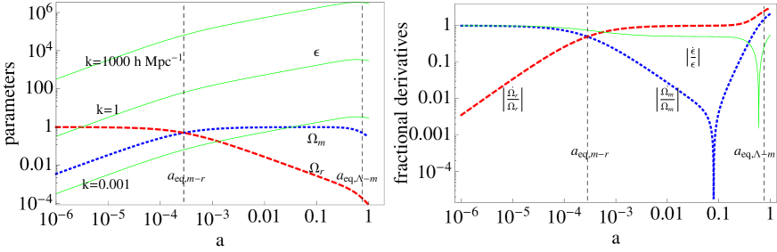
Figure 1: Time dependent parameters in the system. The left panel shows $\Omega_{m}$, $\Omega_{r}$ and the k-dependent $\epsilon$ parameter. Note that at late times $\epsilon$ dominates the other parameters. The right panel shows the fractional derivatives of these quantities, w.r.t. the time variable i.e., $\ln a$. The fractional derivative of $\epsilon$ is the same for all $k$ values considered.

Figure 1 shows the three parameters as a function of time (left panel) and their fractional derivatives (right panel). As can be seen, for a flat cosmology, the density parameters $\Omega_{m}$ and $\Omega_{r}$ stay bounded by unity, whereas, $\epsilon$ keeps increasing for any $k$. For large values of $k$ and/or late epochs, $\epsilon\gg\Omega_{m},\Omega_{r}$. Also, the upper bound on the fractional derivatives for all three parameters is of order unity. We will use these facts when we define the adiabatic condition in §4.

There are three important epochs for this system: the epoch when a given mode crosses the horizon ($a_{hc}$) given by $\epsilon=1$, the epoch of of matter-radiation equality ($a_{eq,m-r}$) given by $\Omega_{m}=\Omega_{r}$ and the epoch of dark energy-matter equality ($a_{eq,\Lambda-m}$) given by $\Omega_{\Lambda}=\Omega_{m}$. These are given by

$$a_{hc}(k) = \frac{k}{H},$$ (12)

$$a_{eq,m-r} = \frac{\Omega_{r,0}}{\Omega_{m,0}}\simeq 2.8\times 10^{-4},$$ (13)

$$a_{eq,\Lambda-m} = \left(\frac{\Omega_{m,0}}{\Omega_{\Lambda,0}}\right)^{1/3}\simeq 0.75,$$ (14)

where the numerical values correspond to the cosmological parameters given in §1.

2.3 Algebraic equation for the potential

Equation (1e) and its transformed version eq. (5e) correspond to the time-time component of Einstein’s equations in the absence of any anisotropic stress. Combining the time-time component with the time-space component gives an algebraic equation for $\Phi$ (e.g., Dodelson 2003):

$$k^{2}\Phi=4\pi Ga^{2}\left[\rho_{m}\delta+4\rho_{r}\Theta_{0}+3\frac{aH}{k}\left(i\rho_{m}v+4\rho_{r}\Theta_{1}\right)\right].$$ (15)

Converting to the $y$-variables defined by eq. 5 and using the definitions of $\epsilon,\Omega_{m}$ and $\Omega_{r}$ given by eqs. (4) and (7), we get

$$y_{5}=B^{-1}\left[4\Omega_{r}\left(y_{1}+\frac{1}{\epsilon}y_{2}\right)+\Omega_{m}\left(y_{3}+\frac{3}{\epsilon}y_{4}\right)\right],$$ (16)

where,

$$B\equiv B(k,a)=3\Omega_{m}+4\Omega_{r}+\frac{2}{3}\epsilon^{2}.$$ (17)

By using eqs. (9), (10) and (11) for the time derivatives of the parameters and eqs. 5a, 5b, 5c and 5d for the time derivatives of the variables, it can be shown that the above form of $y_{5}$ satisfies eq. (5e). Thus, it forms a particular solution for $y_{5}$. The full solution is

$$y_{5}(k,a)=Ce^{-\int_{a_{i}}^{a}\frac{B+2}{2}d\ln a}+B^{-1}\left[4\Omega_{r}\left(y_{1}+\frac{1}{\epsilon}y_{2}\right)+\Omega_{m}\left(y_{3}+\frac{3}{\epsilon}y_{4}\right)\right],$$ (18)

where $C$ is set by the initial conditions. For adiabatic initial conditions of the form given by eqs. 6a, 6b, 6c and 6d and assuming that $\epsilon\ll 1$ gives

$$y_{5}(k,a_{i})\simeq C+y_{5,i}\implies C\simeq 0.$$ (19)

Furthermore, for sub-horizon modes, where $\epsilon\gg 1$, the homogenous term decays exponentially (in terms of the time variable $\ln a$).

Using both the time-time and time-space components of Einstein’s equations is redundant. In the original COSMICS code, one of them was used to check integration accuracy (see discussion in Ma & Bertschinger 1995). Alternatively, it is also possible to substitute the algebraic solution for $y_{5}$ in eqs. (5a) to (5d) to give a 4D dynamical system. Mathematically, this is possible because for adiabatic initial conditions, $C\sim 0$ and physically this means that for scalar perturbations, the Einstein equation is just a constraint equation that does not introduce new propagating degrees of freedom. In appendix §G we compute the eigenvalues of this system. Applying the ideas presented in the rest of this paper, it seems possible that the 4D system may be numerically more stable than the 5D system. However, the advantage of using the algebraic equation for error control may still outweigh the advantage one gains by reducing the dimensionality of the system. A detailed analysis is required to comment more concretely on this issue and whether the results extend to the full Boltzmann system remains to be investigated.

3 Eigenvalue Structure

Before transition	After transition
$\lambda_{1}<0$	$\lambda_{1}<0$
$\lambda_{2}<0$	$\lambda_{2}<0$
$\lambda_{3}<0$	$\lambda_{3}>0$
$\lambda_{4}<0$	$Re[\lambda_{4}]<0$
$\lambda_{5}>0$	$Re[\lambda_{5}]<0$

Table 1: Signs of eigenvalues of ${\mathcal{A}}$. At early times there are four negative roots and one positive root. These transition to two negative, one positive and two complex roots. Figure 2 shows the magnitude of the roots and figure 5 shows the transition epoch.

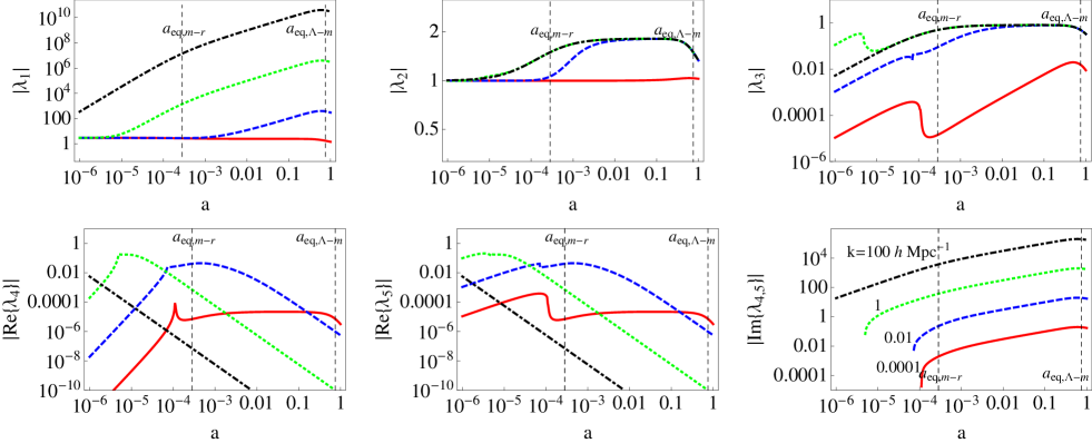
Figure 2: Magnitude of eigenvalues of ${\mathcal{A}}$. The signs are shown in table 1. Four values of $k$ are chosen as shown in the last panel of the bottom row. Kinks in the plots occur at the transition points. $\lambda_{1}$ and $\lambda_{2}$ are smooth through the transition, but the other three change sign or form. The transition for the largest $k$, occurs before $a\sim 10^{-6}$.

Equation (5) can be written in compact form as

$${\dot{\bf y}}={\mathcal{A}}\cdot{\bf y},$$ (20)

where the column vector ${\bf y}=\{y_{1},y_{2},y_{3},y_{4},y_{5}\}$ and the Jacobian matrix ${\mathcal{A}}$ is

$${\mathcal{A}}=\left(\begin{array}[]{ccccc}0&-\frac{\epsilon}{3}&0&0&0\\ \epsilon&0&0&0&-2\epsilon\\ 0&0&0&-\epsilon&0\\ 0&0&0&-1&-\epsilon\\ 2\Omega_{r}&0&\frac{\Omega_{m}}{2}&0&-\frac{B+2}{2}\\ \end{array}\right)$$ (21)

The matrix ${\mathcal{A}}$ has five eigenvalues which depend on $k$ and on time. Although ${\mathcal{A}}$ is a sparse matrix, it has no special symmetries. Hence calculating its eigenvalues analytically is rather cumbersome. Instead we compute them numerically. We find that for each value of $k$, all eigenvalues are real at a sufficiently early time: four of them are negative and one is positive. Eventually there is a transition after which three are real, of which two are negative and one is positive, and two are complex with negative real parts. The positive eigenvalue denotes a growing mode and a negative eigenvalue denotes a decaying mode. The eigenvalue structure is summarized in table 1 and the temporal evolution of the magnitudes for four values of $k=0.001,0.01,1$ and $100$ $h$ ${\rm Mpc}^{-1}$ is plotted in figure 2. Note from the table that $\lambda_{3}$ stays real, but changes sign after the transition. $\lambda_{4}$ and $\lambda_{5}$ become complex; the real part of $\lambda_{5}$ changes sign. Thus, one eigenvalue is always positive throughout the evolution. This is expected since gravitational instability is inbuilt in the E-B system. In figure 2, the kinks in the plots corresponding to $\lambda_{3}$ and real parts of $\lambda_{4}$ and $\lambda_{5}$ mark the epoch of transition. It is clear that the transition epoch is different for each value of $k$.

4 The adiabatic conditions

The E-B system is non-autonomous because the matrix ${\mathcal{A}}$ is time-dependent. Non-autonomous systems are significantly more complicated because there the usual tools used to analyze autonomous systems cannot be applied. For example, analyzing the eigenvalues for such systems to understand the stability can be mis-leading. However, it is always true that, for a linear system, the presence of complex eigenvalues signals an oscillatory behaviour. In §5 we will obtain an analytic prediction for this transition epoch. Another application of the eigenvalue analysis is to predict the stability of numerical schemes. In §6 we investigate the stability of some popular numerical schemes applied to linear autonomous and non-autonomous systems. Dealing with the latter is significantly more involved. This motivates the need to define the adiabatic regime, where the system’s parameters vary slowly enough so that the system becomes ‘quasi-autonmous’ and one can apply the results from the autonomous case.

The E-B system as defined through eq. (20) consists of five dependent variables ($y_{i}$), the independent temporal variable ($\ln a$) and the Jacobian matrix ${\mathcal{A}}$ which is a function of three time-dependent parameters ($\epsilon,\Omega_{m}$ and $\Omega_{r}$). The system can be considered quasi-autonomous if the matrix ${\mathcal{A}}$ varies slowly as compared to the variables or alternately, the fractional change in the matrix in time $dt$ is small compared to the change in the dependent variables. The matrix ${\mathcal{A}}$ can be characterised either by the three parameters or by its five eigenvalues. The variation of the variables defines five time scales $y_{i}/{\dot{y}_{i}}$. If ${\mathcal{A}}$ is characterised by its parameters, the change in ${\mathcal{A}}$ gives three time scales $\epsilon/{\dot{\epsilon}},\Omega_{m}/{\dot{\Omega}_{m}}$ and $\Omega_{r}/{\dot{\Omega}_{r}}$ whereas if it is characterised by its eigenvalues change in ${\mathcal{A}}$ gives five time scales $\lambda_{i}/{\dot{\lambda}_{i}}$. As we shall see below, the two descriptions give different adiabatic conditions.

1. Adiabatic condition based on parameters: We demand that for the system to be ‘quasi-autonomous’, the fractional change in parameters in time $dt$ is small compared to the fractional change in the dependent variables. Refer to eq. (5). Assuming that all the dependent variables $y_{i}$ have the same order of magnitude, it is clear that when $\epsilon\ll 1$, the fractional change ${\dot{y}}_{i}/y_{i}$ is of order unity (note that $\Omega_{m},\Omega_{r}$ are always bounded by unity) and when $\epsilon\gg 1$, ${\dot{y}}/{y}\sim\epsilon$. Thus, to a good approximation ${\dot{y}}/y\sim\max\{1,\epsilon\}$. The adiabatic condition can thus be expressed as

   $$\max\{1,\epsilon\}\gg\max\left\{\left|\frac{\dot{\epsilon}}{\epsilon}\right|,\left|\frac{\dot{\Omega}_{m}}{\Omega_{m}}\right|,\left|\frac{\dot{\Omega}_{r}}{\Omega_{r}}\right|\right\}.$$ (22)

   The $\max$ on the r.h.s. is necessary to guarantee that all the parameters vary slower than the variables. We can thus define a first ‘adiabatic parameter’ $p_{1}$ as the ratio

   $$p_{1}(k,a)=\frac{\max\left\{\left|\frac{\dot{\epsilon}}{\epsilon}\right|,\left|\frac{\dot{\Omega}_{m}}{\Omega_{m}}\right|,\left|\frac{\dot{\Omega}_{r}}{\Omega_{r}}\right|\right\}}{\max\{1,\epsilon\}}.$$ (23)

   As a threshold value, we demand that the function varies at least ten times faster than the variation in the parameters i.e. $p=0.1$.

   An alternate analytic expression for $p_{1}$ can be derived as follows. Referring back to figure 1, we see that the fractional change in the parameters for all epochs is roughly of order unity. Thus, when $\epsilon\ll 1$, which happens at early times and/or for very small $k$, eq. (22) is never satisfied and the adiabatic condition cannot be implemented. When $\epsilon\gtrsim 1$, the denominator of eq. (23) can be replaced by $\epsilon$. To estimate the numerator, note that, until about matter-radiation equality, the fractional derivative of $\epsilon$ (which is equal to that of $\Omega_{m}$) dominates the $\Omega_{r}$ derivative. After the equality, $\Omega_{r}$ derivative starts to dominate. However, in this regime, the value of $\Omega_{r}$ is diminishing. Similarly, far into the matter dominated era, the matter derivative becomes larger, but in this regime $\epsilon$ is very large for most $k$ values of interest. Thus, in the regime where the $\Omega_{m}$ and $\Omega_{r}$ derivatives are dominant, the parameters themselves are sub-dominant and one can replace the numerator of eq. (23) with ${\dot{\epsilon}}/{\epsilon}$. Using eq. (9) to substitute for ${\dot{\epsilon}}/\epsilon$ gives

   $$p_{1,{\rm approx}}(k,a)\approx\frac{1}{\epsilon(k,a)}\left|1-\frac{1}{2}\left(3\Omega_{m}(a)+4\Omega_{r}(a)\right)\right|\;\;\;\ {\rm when}\;\;\epsilon\gtrsim 1$$ (24)

   Figure 3 (left panel) shows the numerically evaluated parameter $p_{1}$ for five values of $k$ using eq. (23). The dashed line corresponds to $p_{1}=0.1$ For each $k$, the point where the curve intersects the dotted line denotes the epoch after which the adiabatic approximation is valid. For small wavenumbers ($\sim 10^{-4}$), the system is never adiabatic until the present epoch; as $k$ increases the range of epochs where the adiabatic approximation is valid increases. The right panel of the same figure shows the contour $p_{1,{\rm approx}}(k,a)=0.1$ (red dotted line) on the $k-a$ plane. The four coloured dots in both panels correspond to the points $p_{1}(k,a)=0.1$ numerically evaluated using eq. (23). It is clear that eq. (24) forms a good approximation for $p(k,a)$.

   

   

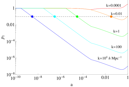
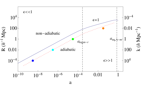
   Figure 3: Adiabatic condition based on parameters. The left panel shows the adiabatic parameter $p_{1}$ as defined in eq. (23) for four values of $k$. The dotted line corresponds to our threshold value of $p_{1}=0.1$ i.e., parameters should vary at least ten times slower than the variables. The resulting ‘adiabatic regime’ lies to the left of the dotted line. The right panel shows the same condition on the $k-a$ plane (red dashed line), but uses the approximate analytic formula given in eq. (24). In both panels, the four points in orange, green, cyan and blue mark the condition $p_{1}(k,a)=0.1$, where $p_{1}$ is numerically evaluated using eq. (23). Thus, the formula of eq. (24) is a fairly good approximation for $p_{1}$. The right panel also shows that imposing an ‘adiabatic regime’ for super-horizon modes is not feasible.

2. Adiabatic condition based on eigenvalues: In the eigenbasis

   $${\dot{\hat{y}}}_{i}=\lambda_{i}{\hat{y}}_{i},$$ (25)

   where the $\hat{}$ denotes eigenvectors. In this case, we demand that for the system to be ‘quasi-autonomous’ the rate of fractional change in the eigenvalues is slow compared to the rate of fractional change in the eigenvectors. This condition can be implemented in two ways. For each eigen-direction one can demand ${\dot{\hat{y}}_{i}}/{\hat{y}}_{i}\gg{\dot{\lambda}}_{i}/\lambda_{i}$. Alternatively, a more conservative way is to demand that the smallest time scale of change in eigenvalues $\min\{|{\dot{\lambda}}_{i}/\lambda_{i}|^{-1}\}$ is larger than the largest time scale of change in eigenvectors $\max\{|{\dot{\hat{y}}_{i}}/{\hat{y}}_{i}|^{-1}\}$. Noting that, the rate of fractional change in the eigenvector is given by ${\dot{y}}/y\sim\lambda$, we define two other adiabatic parameters:

   $$p_{2,A}(k,a) = \max\left\{\left|\frac{{\dot{\lambda}}_{i}}{\lambda_{i}^{2}}\right|\right\}$$ (26)

   $$p_{2,B}(k,a) = \frac{\max|{\dot{\lambda}}_{i}|}{\min\{|\lambda_{i}|\}},$$ (27)

   where the latter is a more conservative definition. Figure 4 shows the two parameters as a function of $k$ and $a$. The dashed line indicates the condition $p_{2,A/B}=0.1$. It is clear that these conditions are significantly more restrictive than the earlier condition of adiabaticity defined in terms of the parameters.

   

   

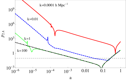
   Figure 4: Adiabatic conditions in the eigenbasis. The left and right panels show the adiabatic parameter as defined in eqs. (26) and (27) respectively. The dashed line in both plots denoted the condition $p_{2,A/B}=0.1$. While in the first case there is a small ‘adiabatic range’, there is no appropriate range in the second definition. Overall, these are far more restrictive parameters than the adiabatic regime based on parameters.

Which definition of ‘adiabaticity’ is appropriate depends upon the problem at hand. One can imagine evolving the E-B system by transforming to the eigenbasis. In this case, the evolution in the adiabatic regime will be given simply by the exponential of the diagonal matrix of eigenvalues. However, in this paper, in §8, we construct solutions in the basis defined by eq. (20). Hence, in this paper, we will use the first adiabatic condition characterised in terms of the parameter $p_{1}$.

5 Onset of oscillations

It was shown in §3 that the five eigenvalues of the matrix ${\mathcal{A}}$ undergo a transition from all real to three real and two complex. The epoch at which the transition takes place depends upon $k$. Although the eigenvalues are not known analytically, it is possible to analytically predict this epoch of transition. The method involves applying Sturm’s theorem and Descartes’ rule of sign to the characteristic polynomial of ${\mathcal{A}}$ and has been explained in detail in appendix B. This analysis implies that the $k$-dependent transition epoch $a_{trans}$ is the solution of

$$9\Omega_{m}(a_{trans})+2\left[3-6\Omega_{r}(a_{trans})+\epsilon(a_{trans},k)^{2}\right]=0.$$ (28)

Figure 5 shows the scale that transitions to complex eigenvalues as a function of $a$. The figure suggests that, for all scales, the transition epoch occurs before the epoch of matter-radiation equality $a_{eq,m-r}$. This may seem counter-intuitive because, in general, no oscillations are expected for scales that enter the horizon after $a_{eq,m-r}$ i.e., for $k\ll k_{eq}$. However, note that Sturm’s analysis does not predict the actual value of the frequency of oscillations. This is determined by the imaginary part of the eigenvalue, which in the large $\epsilon$ limit (late epochs) reduces to $\epsilon/\sqrt{3}$ and is smaller for earlier epochs (see figure 15 in appendix §C). For $k\sim 0.1k_{eq}$, the average $\epsilon\sim 0.1$ in the interval from equality to today. In this interval, which corresponds to about 8 e-folds, one expects, $\sim 8\times 0.1/\sqrt{3}\approx 0.5$ oscillations i.e., about half an oscillation. This issue is explained in greater detail in appendix §C. For smaller values of $k$, this number will be even smaller and hence no oscillations are visible. It is also interesting to note that for modes with $k\gtrsim 0.1$ $h$ ${\rm Mpc}^{-1}$, the epoch of transition almost coincides with the epoch of horizon crossing. This means that, soon after the transition the oscillation frequency is of order unity or smaller: the regime of high frequency oscillations, which is numerically difficult to track, occurs well after the transition epoch.

As was discussed earlier, for a linear autonomous system complex eigenvalues imply oscillations and vice versa. For linear non-autonomous systems too, complex eigenvalues imply oscillations, however, the converse need not be true. Thus the transition to complex eigenvalues, in principle, indicates the presence of oscillations, not necessarily their onset. However, numerically, we do not find any evidence of oscillatory solutions before the epoch of transition for any value of $k$. Thus, we consider the transition epoch to denote the onset of oscillations.

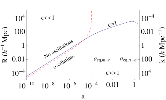
Figure 5: Onset of oscillations: the transition from real to complex roots is denoted by the red dashed line. The blue solid line denotes the epoch of horizon crossing. It is clear that for most scales the onset of oscillations occurs very early, much before the epoch of matter-radiation equality.

6 Numerical Stability

Given an initial value problem to be solved numerically, there are many parameters that dictate the choice of an integration scheme. Apart from accuracy and available computing time, one important criterion is the stability of the numerical scheme. Loosely speaking, stability refers to the ability of the numerical solution to track the qualitative behaviour of the analytical solution. For example, if the analytic solution is bounded or converges to zero, the numerical approximation should also exhibit this behaviour. Mathematically, this property is characterised in terms of a function $r(z)$ called the stability function and the stability criterion is

$$|r(z)|\leq 1.$$ (29)

For instance, for a one-dimensional differential equation of the type ${\dot{y}}=\lambda y$, the stability function depends only on the step size $h$ and the eigenvalue $\lambda$. Thus, given $\lambda$ and a particular method, one can estimate the allowed step size by applying the stability criterion. It should be noted that such a stability criterion is relevant only when $\lambda$ is negative (or more generally, has negative real part). When $\lambda$ is positive the analytic solution grows exponentially and the choice of step size is dictated by how accurately the numerical solution is expected to track the analytic one. Similarly, if the eigenvalue is complex ($\lambda=i\omega$), the analytic solution oscillates with a frequency $\omega$ and numerically these oscillations can be fully resolved only if $h\leq 2\omega^{-1}$. Thus, for a multi-dimensional system, like the E-B system considered here, the choice of step-size is dictated by a combination of accuracy requirements corresponding to the positive and complex eigenvalues and stability requirements related to the eigenvalues with negative real parts.

In the appendix, we review the basic stability theory (Butcher, 1987; Harrier et al., 1996; Harrier & Wanner, 1996; Petzold & Ascher, 1998) for two classes of integration methods used to solve initial value problems: RK4 schemes and linear multistep methods, in particular the Backward Differentiation Formula (BDF) methods. RK4 schemes are single step schemes (the solution at the $n$-th step denoted by $y_{n}$ depends on the $n-1$-th step) but it can have multiple computations (called as stages) per step. In a linear multistep method with $k$ steps, $y_{n}$ depends linearly on $y_{n-1},y_{n-2}\ldots y_{n-k}$ and/or the derivative at those points. Both RK4 and linear multi-step methods have explicit schemes (where the solution for $y_{n}$ is computed directly from knowing the previous steps) and implicit schemes (where the solution for $y_{n}$ depends on solving a functional equation). Explicit schemes are easier to implement than implicit schemes, but tend to be less stable. Table 2 gives the stability functions for five commonly used methods: forward and backward Euler (these are the simplest first order explicit and implicit schemes), the popular fourth order Runge-Kutta solver (RK4), the trapezoidal rule (which is a second order implicit linear multistep method) and the second order BDF2 scheme. The formula for the third order BDF3 scheme is given in eq. (130) in the appendix D. The order refers to how the error between the approximate and true solution scales as a function of the step size $h$.

Method	Form	Order	Stability function ($z=h\lambda$)
Forward Euler	$y_{n}=y_{n-1}+hf_{n-1}$	1	$r(z)=1+z$
Backward Euler	$y_{n}=y_{n-1}+hf_{n}$	1	$r(z)=\frac{1}{1-z}$
Standard Runge-Kutta	$\begin{array}[]{lcl}y_{n}&=&y_{n-1}+\frac{h}{6}\left(k_{1}+2k_{2}+2k_{3}+k_{4}\right)\\ k_{1}&=&f(x_{n-1},y_{n-1})\\ k_{2}&=&f(x_{n-1}+\frac{h}{2},y_{n-1}+\frac{h}{2}k_{1})\\ k_{3}&=&f(x_{n-1}+\frac{h}{2},y_{n-1}+\frac{h}{2}k_{2})\\ k_{4}&=&f(x_{n-1}+h,y_{n-1}+hk_{3}).\end{array}$	4	$r(z)=1+z+\frac{z^{2}}{2}+\frac{z^{3}}{6}+\frac{z^{4}}{24}$
Implicit Trapezoidal Rule	$y_{n}=y_{n-1}+\frac{h}{2}\left(f_{n}+f_{n-1}\right)$	2	$r(z)=\frac{2+z}{2-z}$
BDF2 (implicit)	$y_{n}=\frac{4}{3}y_{n-1}-\frac{1}{3}y_{n-2}+\frac{2}{3}f_{n}0$	2	$r(z)=\frac{2+\sqrt{1+2z}}{3-2z}$

Table 2: Stability functions for some commonly used numerical schemes. The function and its derivative at the $n$-th step are denoted by $y_{n}$ and $f_{n}$ respectively. For differential equations of the form ${\dot{y}}=\lambda y$, the stability condition is $|r(z=h\lambda)|=1$. Thus, given a $\lambda$, the step size can be determined.

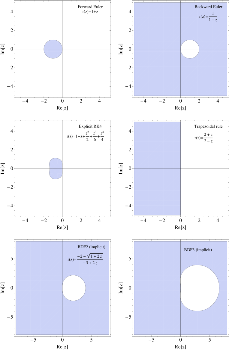
Figure 6: Stability regions for some popular methods in the complex $z=\lambda h$ plane. Shaded regions satisfy the stability condition $|r(z)|\leq 1$. Note that the forward Euler and explicit RK4 are stable in a very small region. The BDF schemes are stable almost everywhere except for a small region in the $z$ plane. The BDF3 scheme has higher order than BDF2 so it is more efficient in terms of convergence, but it has a larger domain where it is unstable. If the eigenvalue $\lambda$ is real and positive, then the stability requirements for implicit methods imply a minimum step size.

Figure 6 shows the stability regions in the complex $z$ plane for each method. It is clear that implicit schemes have a greater region of stability than explicit schemes. For example, compare the forward and backward Euler schemes: in the first case $z=\lambda h$ must lie inside the shaded region in the left half-plane, whereas in the latter case $z=\lambda h$ can be anywhere except inside the non-shaded region in the right half-plane. Thus, for the particular schemes considered here, the stability requirement imposes a maximum allowed step size for explicit schemes and a minimum required step size for implicit schemes. Another feature to note is that sometimes there is a trade-off between order and stability. For example, the last panel implies that the BDF2 scheme has a greater region of stability than the higher order BDF3 scheme.

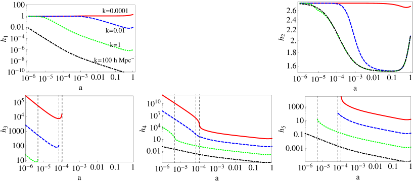
Figure 7: The maximum allowed step size for a RK4 scheme applied to the E-B system. For simplicity, we assume that the system is autonomous and solve for $|r(z)|=1$ to get the minimum $h_{i}$ for each eigenvalue $\lambda_{i}$. Each resulting $h_{i}$ is a function of $k$ and $a$. The dashed vertical lines denote the transition from real to complex values. Refer to table 1 for the signs of the eigenvalues. For positive eigenvalues, the maximum allowed value is zero i.e., the explicit scheme is never stable (third and fifth panel). For high negative values, the step size becomes vanishingly small as shown in the first panel.

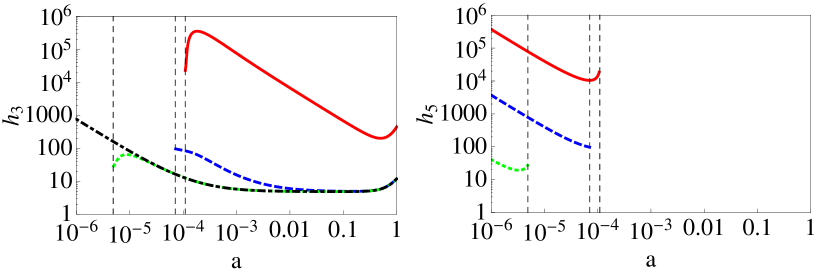
Figure 8: The minimum required step size for the BDF2 scheme. The colour coding is the same as in figure 7. For eigenvalues with negative real part, there is no minimum requirement. The step size can be arbitrary. Thus, only the step sizes $h_{3}$ and $h_{5}$ corresponding to $\lambda_{3}$ and $\lambda_{5}$ are shown here.

We now apply the stability conditions to the E-B system. There are five independent eigendirections and the stability criterion can be applied separately for each of them. Figure 7 shows the case for the explicit RK4 scheme for four $k$ values. For each eigenvalue $\lambda$, we numerically solve $|r(z=h\lambda)|=1$ to get the maximum allowed step size $h$. Note that for the RK4 stability function, this gives only two real roots: $\lambda h=-2.785$ and $\lambda h=0$. Thus, if $\lambda$ is positive, the explicit RK4 scheme cannot work; the maximum allowed step size is zero. Figure 7 can be understood in conjunction with table 1. $\lambda_{1}$, $\lambda_{2}$ are always real and negative and hence give a positive solution for $h$. $\lambda_{3}$ is negative until the transition point, after which it is positive. So $h_{3}$ is positive until the transition and zero thereafter. $\lambda_{4}$ is negative until the transition after which it is complex with a negative real part; thus for a real positive $h$, $z=\lambda h$ will lie in the second quadrant. Since the region of stability extends in this part of the plane, even complex eigenvalues give a real $h$. On the other hand, $\lambda_{5}$ is positive before the transition and hence the only solution in this part is $h_{5}=0$; after the transition, the solution for $h_{5}$ is identical to $h_{4}$ since the region of stability is symmetric about the $x$-axis.

This can be contrasted with the behaviour of an implicit scheme applied to the same system. Figure 8 shows the minimum required step size from the stability condition $|r(z)|=1$ for the BDF2 scheme. Since $\lambda_{1},\lambda_{2}<0$ and $Re(\lambda_{4})<0$ for all epochs, there is no restriction on the step size, i.e., the scheme is always stable for evolution along these eigendirections. $\lambda_{3}$ ($\lambda_{5}$) is positive after (before) the transition which translates into a minimum required $h_{3}$ and $h_{5}$ in these regimes. Notice that the step-size is rather large; the total interval of integration (from $a\sim 10^{-8}$ to $a=1$) is about 18 e-folds, and thus much smaller than the minimum required step size. What does such a large stepsize mean ? This issue is also present in the case of explicit schemes, where stability requirements implied a zero step size for positive eigenvalues. This is expected. The stability criterion is derived from the condition that the numerical solution should decay when the analytic solution does so (see §D). Thus, as noted earlier, it is relevant only to the sub-space of the system whose eigenvalues have negative real parts. The E-B system has gravitational instability encoded in it and some component of the solution is always growing which plausibly manifests as a positive eigenvalue. In practice, for positive eigenvalues, the step size is dictated by accuracy considerations rather than stability, since the numerical as well as analytic solutions are unstable.

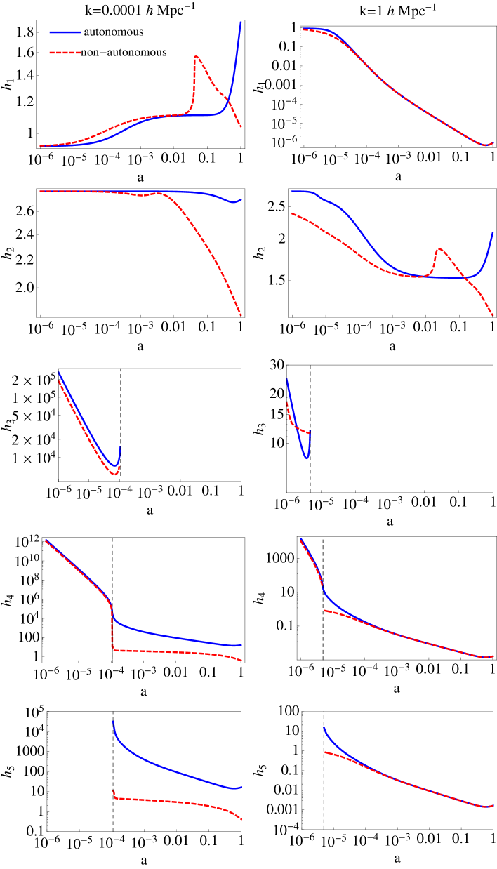
Figure 9: Comparison of step sizes for a explicit RK4 scheme derived using the autonomous (blue solid) and non-autonomous (red dashed) stability condition for $k=0.0001$ $h$ ${\rm Mpc}^{-1}$ (left) and $k=1$ $h$ ${\rm Mpc}^{-1}$ (right). The vertical dashed lines indicate the epoch of transition to complex values for each value of $k$.

As discussed earlier, the E-B system is non-autonomous. For a non-autonomous system the eigenvalue $\lambda$ is a function of the time variable and the stability function needs to be generalized. As an example, we consider the RK4 method applied to the non-autonomous system. If $x$ is the independent variable ($\ln a$ in the E-B case) then the stability function is (Burrage & Butcher, 1979)

$$R(h,x)=1+\frac{z_{1}}{6}+\frac{z_{2}}{3}+\frac{z_{1}z_{2}}{6}+\frac{z_{3}}{3}+\frac{z_{2}z_{3}}{6}+\frac{z_{1}z_{2}z_{3}}{12}+\frac{z_{4}}{6}+\frac{z_{3}z_{4}}{6}+\frac{z_{2}z_{3}z_{4}}{12}+\frac{z_{1}z_{2}z_{3}z_{4}}{24},$$ (30)

where the $z_{i}$s are functions of the eigenvalues evaluated at the sub-grid points defined by the nodes ($c$ values in the Butcher tableau):

$$z_{1} = h\lambda(x)$$ (31)

$$z_{2} = h\lambda(x+\frac{h}{2})$$ (32)

$$z_{3} = h\lambda(x+\frac{h}{2})$$ (33)

$$z_{4} = h\lambda(x+h).$$ (34)

The stability condition is unchanged:

$$|R(h,x)|\leq 1.$$ (35)

Figure 9 shows the step sizes derived using the autonomous (solid blue line) and non-autonomous (dashed red line) conditions for two values $k=0.0001$ (left column) and $k=1$ $h$ ${\rm Mpc}^{-1}$ (right column). We find that except when the eigenvalues are complex, the step size in the autonomous and non-autonomous cases are comparable. For example, for $k=0.0001$ $h$ ${\rm Mpc}^{-1}$, the plots of $h_{1}$ and $h_{2}$ in the two cases almost overlap for $a\lesssim 0.01$. They differ in the case of complex eigenvalues (for example $h_{4}$ and $h_{5}$ after the transition) but the difference is less for larger values of $k$. This can be understood from the adiabatic conditions discussed in §4, where we show that in an appropriately defined ‘adiabatic’ regime, the system can be considered autonomous. Larger values of $k$ satisfy the adiabatic condition for a longer range of epochs. Thus, in practice, it may be possible to use the stability analysis for autonomous systems to determine the step size and the non-autonomous nature can be accounted by making a conservative choice. For appropriate values of $k$, this strategy is further supported by the adiabatic conditions.

7 Stiffness

A differential equation is generally considered to be stiff if there are two or more widely separated time scales in the problem. For the EB system without baryons the two scales are the oscillation time scale of a photon mode and the Hubble time. In terms of the conformal time these are $\eta_{k}=k^{-1}$ and $\eta_{H}\sim(aH)^{-1}$. In the presence of baryons, there is an additional time scale associated with the Thomson scattering of photons and baryons i.e., $\eta_{c}=(an_{e}\sigma_{T})^{-1}$, where $n_{e}$ is the electron density and $\sigma_{T}$ is the collisional cross section. In appendix F we recast the system with $\ln a$ as the time variable and show that that the three time scales appear as two ratios: $\epsilon_{k}=\eta_{H}/\eta_{k}\sim k/aH$ and $\epsilon_{c}=\eta_{H}/\eta_{c}\sim(an_{e}\sigma_{T})/(aH)$ ($\epsilon_{k}=\epsilon$ in the rest of this text; we use the subscript only while considering the full system). For early epochs, before recombination, the Thomson opacity is large and the photons and baryons are tightly coupled i.e., $\eta_{c}<<\eta_{H}$ or $\epsilon_{c}\gg 1$. This regime is usually handled by invoking the tight coupling approximation. There are various implementations of this approximation (referred to as TCA; see Blas, Lesgourgues, & Tram 2011) all of which effectively re-write the coupling term such that the resulting equations are independent of $\eta_{c}^{-1}$. Another regime where the system becomes numerically difficult to track is when $\epsilon_{k}$ is large i.e., when the photon moments undergo rapid oscillations. However, for most modes of interest, this occurs at late epochs well into the matter or dark energy dominated phase and the radiation fields need not be tracked with high accuracy. Practically, the radiation streaming approximation (referred to as RSA in the second CLASS paper) is invoked wherein one substitutes approximate analytic expressions for the radiation fields thus circumventing the problem of numerically tracking them. This approximation has been discussed by Doran 2005b in the conformal Newtonian Gauge and by Blas, Lesgourgues, & Tram 2011 in the synchronous gauge.

In the CMB literature, only the tight coupling regime is usually referred to as the ‘stiff’ regime. But, it is clear that $\eta_{c}<<\eta_{H}$ and $\eta_{k}<<\eta_{H}$ are both regimes where there are two widely separated time scales in the problem and the system is stiff. Hence one of the aims in this paper is to understand better the definition of ‘stiffness’ and discuss means to characterise it. Stiff systems have multiple time scales spanning a large dynamic range. To maintain stability of the solution, it is usually necessary that the step size be smaller than the smallest time scale in the system, even though accuracy requirements may allow a larger step size (Press et al., 2002). Thus, a stiff system can be characterised as follows (Petzold & Ascher, 1998). An initial value problem is considered ‘stiff’ over an interval, if the step size required to maintain stability of the forward Euler method is significantly smaller than the step size required to maintain accuracy. Hence, whether a problem is considered stiff or not depends upon: (1) the parameters of the differential equation (2) the accuracy criterion, (3) the length of the interval of integration and (4) the region of absolute stability of the method. For a stiff problem, the step size dictated by stability requirements of an explicit scheme becomes prohibitively small and typically an implicit method needs to be invoked.

In the EB system without baryons there are two physical time scales and their ratio $\epsilon$ primarily governs the rates at which the variables evolve (coefficients of most terms are of the order of $\epsilon$). In the eigenbasis it has the form ${\dot{y}}_{i}=\lambda_{i}y_{i}$, and each eigenvalue has an associated time scale $\lambda_{i}^{-1}$. One way to characterise ‘stiffness’ is to define the ‘stiffness ratio’ $s$ as (Lambert, 1992)

$$s=\frac{|{\mathcal{R}e}\{\lambda_{max}\}|}{|{\mathcal{R}e}\{\lambda_{min}\}|}\;\;\;\;\lambda_{min,max}<0,$$ (36)

where $\lambda_{max}$ and $\lambda_{min}$ denote the most and least negative eigenvalue respectively. Restricting to the subspace of negative eigenvalues is necessary since stability of the numerical solution is defined only in this subspace. Figure 10 (left plot) shows the stiffness parameters defined above as a function of epoch for four values of $k$. It is clear from the figure that the E-B system has a large stiffness ratio for a wide range of $k$ and epochs. The right plot shows the stiffness parameter $s$ vs $\epsilon$. It is seen that the stiffness parameter is minimum when $\epsilon\sim 1$ i.e. when the time scale of oscillation and Hubble evolution are of the same order.

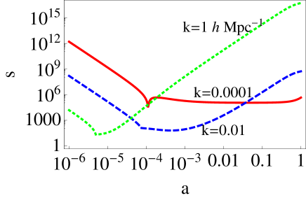
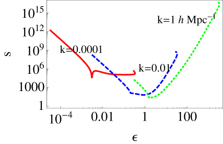
Figure 10: The left plot shows the stiffness parameter defined in the text in eq. (36). Large values of $s$ indicates that the E-B system is ‘stiff’ at all epochs for all modes. Thus, implicit methods have to be employed since explicit methods are expected to be unstable for such systems. The right plot shows $s$ vs. $\epsilon$. Even for super-horizon modes with small values of $\epsilon$, the system is stiff.

In the past implicit schemes have been advocated to evolve the full system E-B system including baryons, particularly to treat the tight coupling regime. For example, CLASS uses the solver ndf15 which is a Numerical Differentiation Formula (NDF) very closely related to the BDF methods (Shampine & Reichelt, 1997). CAMB, on the other hand, uses the DVERK routine, which is based on higher order (adaptive) Runge-Kutta methods and is most efficient for non-stiff systems (see subroutines.f90 of the CAMB sourcecode). However, due to the various approximations (TCA and RSA) to treat the stiff regimes this does not prove to be prohibitive.

8 Limits

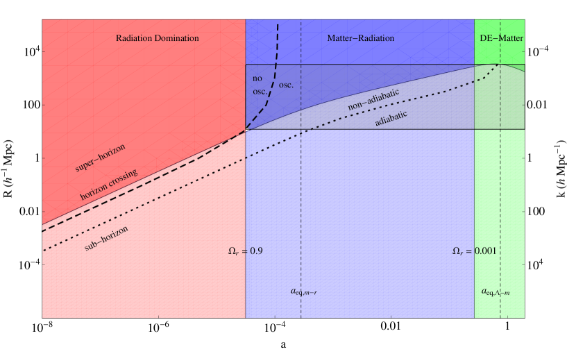
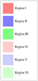
Figure 11: Various regions on the ‘$k-a$’ plane. The dot-dashed line separates the regions where the eigenvalues are real (no oscillations) from where they are complex (onset of oscillatory behaviour). The dashed line indicates the regions where the adiabatic condition holds and the system can be treated as an autonomous system. The regions marked I to VI indicate various limits where analytic solutions are available to test numeric codes. We choose the end of radiation domination to be the epoch when $\Omega_{r}=0.9$ and the beginning of the matter-dark energy era when $\Omega_{r}=0.001$. The shaded rectangle indicates the range of $k$ values where a complete solution cannot be constructed. This range is from $k=0.1$ to $k=3.\times 10^{-4}$ $h$ ${\rm Mpc}^{-1}$.

There are three parameters in the E-B system: $\Omega_{m}$, $\Omega_{r}$ and $\epsilon$. Based on the value of $\epsilon$ there are two different regimes: superhorizon ($\epsilon\ll 1$) and sub-horizon ($\epsilon\mathbin{\lower 3.0pt\hbox{$\hbox to0.0pt{\raise 5.0pt\hbox{$\char 62\relax$}\hss}\mathchar 29208\relax$}}1$ and $\epsilon\gg 1$). Based on the $\Omega$ parameters the evolution can be classified into three eras: the radiation domination when $\Omega_{m}\ll\Omega_{r}0$, the matter-radiation era, when both $\Omega_{m}$ and $\Omega_{r}$ are non-zero and the matter-dark energy era when $\Omega_{r}\ll\Omega_{m}$ and $1-\Omega_{m}-\Omega_{r}=\Omega_{\Lambda}$. This classification defines six separate regions (denoted by the roman numerals ‘I’ to ‘VI’) where analytic forms can be obtained. Figure 11 shows these regions along with a summary of the various regimes given by the eigenvalue analysis discussed in earlier sections. We have chosen $\Omega_{r}=0.9$ to be the end of radiation domination and $\Omega_{r}=0.001$ to be the onset of the matter-dark energy era. The solutions in these different regions are listed below. The details involved in arriving at these forms are given in appendix E. The solutions depend on initial conditions denoted by subscript ‘$i$’. These initial conditions are in general different for each region . This allows one to compare the solutions in each region independently.

8.1 Analytic forms

There has been extensive work in the past in terms of obtaining solutions to the Boltzmann system, for example, super-horizon solutions have been constructed by Kodama & Sasaki (1984) and extensive work has been done in the sub-horizon regime by Hu and collaborators (for e.g., Hu & Sugiyama 1995, 1996). In this paper we obtain solutions in terms of the variables $y_{1}$ to $y_{5}$. In some cases we can reproduce earlier results, while in others there is a slight difference because of the change of variables.

• Region I: super-horizon modes in the radiation domination era
  To the lowest order in $\epsilon$, the first four variables in this region of the $k-a$ plane become

  $$y_{1}(a) \simeq y_{1,i}$$ (37a)

  $$y_{2}(a) \simeq y_{2,i}$$ (37b)

  $$y_{3}(a) \simeq y_{3,i}$$ (37c)

  $$y_{4}(a) \simeq\frac{y_{4,i}a_{i}}{a}$$ (37d)

  The solution for $y_{5}$ in regions I, II and III is derived assuming that $y_{1}$ and $y_{3}$ are constants. In both region I and II, the solution for $y_{5}$ is expressed in terms of the variable

  $$x=\frac{a}{a_{eq,m-r}},$$ (38)

  where $a_{eq,m-r}$ is the epoch of radiation-matter equality. For adiabatic initial conditions set at inflation, and assuming a very small $x_{i}\ll 1$, the solution for $y_{5}$ is the well-known solution (Kodama & Sasaki, 1984).

  $$y_{5}(a)\equiv y_{5}(x)=\frac{y_{5,i}}{10}\left(16\frac{\sqrt{1+x}}{x^{3}}-\frac{16}{x^{3}}-\frac{8}{x^{2}}+\frac{2}{x}+9\right).$$ (39)

  It is possible to get refined approximations for $y_{1}$ to $y_{4}$ using the solutions given by eqs. 37a, 37b, 37c and 37d and eq. (39) and in the r.h.s. of eqs. 5a, 5b, 5c and 5d and integrating the resulting system. This gives,

  $$y_{1}(k,a) =y_{1,i}-y_{2,i}\int_{a_{i}}^{a}\frac{\epsilon(k,a^{\prime})}{3}d\ln a^{\prime}$$ (40a)

  $$y_{2}(k,a) =y_{2,i}+y_{1,i}\int_{a_{i}}^{a}\epsilon(k,a^{\prime})d\ln a^{\prime}-2\int_{a_{i}}^{a}y_{5}(a^{\prime})\epsilon(k,a^{\prime})d\ln a^{\prime}$$ (40b)

  $$y_{3}(k,a) =y_{3,i}-y_{4,i}a_{i}\int_{a_{i}}^{a}\frac{\epsilon(k,a^{\prime})}{a^{\prime}}d\ln a^{\prime}$$ (40c)

  $$y_{4}(k,a) =\frac{y_{4,i}a_{i}}{a}-\frac{1}{a}\int_{a_{i}}^{a}a^{\prime}\epsilon(k,a^{\prime})y_{5}(a^{\prime})d\ln a^{\prime}.$$ (40d)

  Deep in the radiation dominated era, $\epsilon\sim a$ and the integrals can be evaluated analytically (see appendix E).

• Region II: super-horizon modes in the radiation-matter era
  The main difference between region I and II is that the initial conditions in the latter are not necessarily those that are set by inflation. The super-horizon mode evolves through the radiation dominated era before entering region II and and variables change as a result of this evolution. The general solution for $y_{5}$ in terms of the variable $x$ defined in eq. (38) is

  $$y_{5}(x)=\frac{\sqrt{1+x}}{x^{3}}\left(\frac{y_{3,i}}{5}\left.\left\{\frac{16+8x-2x^{2}+x^{3}}{\sqrt{1+x}}\right\}\right|_{x_{i}}^{x}+\frac{4y_{1,i}}{3}\left.\left\{\frac{-8-4x+x^{2}}{\sqrt{1+x}}\right\}\right|_{x_{i}}^{x}\right)+y_{5,i}\left(\frac{x_{i}}{x}\right)^{3}\sqrt{\frac{1+x}{1+x_{i}}}.$$ (41)

  Note that this equation reduces to eq. (39) for $x_{i}\ll 1$ and initial conditions given by eqs. 6a, 6b, 6c and 6d.

  The solutions for $y_{1}$ to $y_{4}$ have the same functional form as eqs. 40a, 40b, 40c and 40d but the integrals should be solved numerically with the appropriate values of the initial conditions.

• Region III: super-horizon modes in the matter-dark energy era.
  In this region, the functional form of the solutions for $y_{1}$ through $y_{4}$ are the same as in region I and II and given by eqs. 40a, 40b, 40c and 40d. $y_{5}$ is solved in terms of the variable

  $$x=a/a_{eq,\Lambda-m},$$ (42)

  where $a_{eq,\Lambda-m}$ is the epoch of matter-dark energy equality. The solution for $y_{5}$ in region III in terms of $x$ and the initial value $x_{i}$ is given by a hypergeometric function (Arfken 2000):

  $$y_{5}(x,x_{i})=C\frac{\sqrt{1+x^{3}}}{x^{5/2}}-\frac{y_{3,i}}{4}\frac{1}{x^{5/2}(1+x^{3})^{1/6}}\;\;{}_{2}F_{1}\left(\frac{2}{3},\frac{1}{6},\frac{5}{3},\frac{1}{1+x^{3}}\right),$$ (43)

  where

  $$C=y_{5,i}\frac{x_{i}^{5/2}}{\sqrt{1+x_{i}^{3}}}+\frac{y_{3,i}}{4}\frac{1}{(1+x_{i}^{3})^{2/3}}\;\;{}_{2}F_{1}\left(\frac{2}{3},\frac{1}{6},\frac{5}{3},\frac{1}{1+x_{i}^{3}}\right).$$ (44)

• Region IV: sub-horizon modes in the radiation dominated era
  Let us define

  $$x=\epsilon/\sqrt{3}.$$ (45)

  In this region we then obtain

  $$y_{1}(x) =-\frac{1}{2x}\left[(a_{2}x-2a_{1})\sin x+(a_{1}x+2a_{2})\cos x\right]$$ (46a)

  $$y_{2}(x) =-\frac{\sqrt{3}}{2x^{2}}\left[\left\{2a_{2}x+a_{1}\left(x^{2}-2\right)\right\}\sin x+\left\{2a_{1}x-a_{2}\left(x^{2}-2\right)\right\}\cos x\right]$$ (46b)

  $$y_{3}(x) =3a_{1}\left.\left(\frac{\sin x}{x}+\ln x\frac{\sin x_{i}}{x_{i}}-\text{Ci}(x)\right)\right|_{x_{i}}^{x}-3a_{2}\left.\left(\frac{\cos x}{x}+\ln x\frac{\cos x_{i}}{x_{i}}+\text{Si}(x)\right)\right|_{x_{i}}^{x}-\sqrt{3}y_{4,i}x_{i}\ln\left(\frac{x}{x_{i}}\right)+y_{3,i}$$ (46c)

  $$y_{4}(x) =-\frac{\sqrt{3}}{x^{2}x_{i}}\left[a_{1}(x\sin x_{i}-x_{i}\sin x)+a_{2}(x_{i}\cos x-x\cos x_{i})\right]+\frac{y_{4,i}x_{i}}{x}$$ (46d)

  $$y_{5}(x) =a_{1}\left(\frac{\sin x-x\cos x}{x^{3}}\right)-a_{2}\left(\frac{x\sin x+\cos x}{x^{3}}\right),$$ (46e)

  where

  $$\text{Ci}(x)=-\int_{x}^{\infty}\frac{\cos x^{\prime}}{x^{\prime}}dx^{\prime}\;\;\;{\rm and}\;\;\;\text{Si}(x)=\int_{0}^{x}\frac{\sin x^{\prime}}{x^{\prime}}dx^{\prime}.$$ (47)

  Here $a_{1}$ and $a_{2}$ are determined by initial conditions. Either one can determine them using the initial conditions of $y_{1}$ and $y_{2}$ in eqs. (46a) and (46b). Alternatively, one can demand that at early times $y_{5}$ tends to a constant ($y_{5,i}$). For adiabatic initial conditions set up at a early time $a_{i}\sim 10^{-8}$, these two are equivalent and effectively give $a_{1}=3y_{5,i}$ and $a_{2}=0$. In a more general case, the solution for $y_{5}$ contains a contribution from the homogenous part of the differential equation, eq. (5e), with an unknown constant. In this case, $a_{1}$, $a_{2}$ and the unknown constant are jointly set using the initial conditions on $y_{1},y_{2}$ and $y_{5}$.

  Note that in the radiation dominated era, $\epsilon=\eta$, $x=k\eta/\sqrt{3}$ and the solution for $y_{5}$ is the usual Bessel function solution for $\Phi$. The variable $y_{3}$ has a logarithmic dependence on $x$; this is similar to the logarithmic dependence of $\delta$ in the sub-horizon solution of Hu & Sugiyama (1996).

• Region V: sub-horizon modes in the radiation-matter era
  In this region, the evolution for $y_{3}$ for most modes of interest happens to be scale-independent (i.e., does not depend on $\epsilon$). The remaining four variables, however, do depend on $k$. In solving for $y_{3}$, it is assumed that $y_{5}$ depends only on the matter variables, however, having solved for $y_{1}$ to $y_{4}$, a complete solution for $y_{5}$ can be constructed eq. (16). This ‘second order’ solution that includes the effect of radiation on the potential is more accurate than the solution which ignores the radiation.

  $$y_{1}(k,a) = c_{1}\cos I(k,a)+c_{2}\sin I(k,a)+a_{3}y_{3}(a)$$ (48)

  $$y_{2}(k,a) = \sqrt{3}\left(c_{1}\sin I(k,a)-c_{2}\cos I(k,a)\right)+b_{4}y_{4}(k,a)$$ (49)

  $$y_{3}(a) = c_{3}\left(x+\frac{2}{3}\right)+c_{4}\left[\left(x+\frac{2}{3}\right)\log\left(\frac{\sqrt{1+x}+1}{\sqrt{1+x}-1}\right)-2\sqrt{1+x}\right]\;\;\;{\rm where}\;\;x=a/a_{eq,m-r}$$ (50)

  $$y_{4}(k,a) = -\frac{1}{\epsilon(k,a)}\left\{c_{3}x+c_{4}\left[x\log\left(\frac{\sqrt{1+x}+1}{\sqrt{1+x}-1}\right)-\frac{2(1+3x)}{3\sqrt{1+x}}\right]\right\}$$ (51)

  $$y_{5}(k,a) = \frac{1}{B(k,a)}\left[4\Omega_{r}\left(y_{1}+\frac{y_{2}}{\epsilon}\right)+\Omega_{m}\left(y_{3}+\frac{3y_{4}}{\epsilon}\right)\right],$$ (52)

  where

  $$I(k,a)=\int_{a_{i}}^{a}\frac{\epsilon(k,a^{\prime})}{\sqrt{3}}d\ln a^{\prime},$$ (53)

  $$a_{3}=\frac{2\Omega_{m}}{B+3\Omega_{m}},\;\;\;b_{4}=\frac{6\Omega_{m}}{B+3\Omega_{m}}.$$ (54)

  and $c_{1},c_{2},c_{3},c_{4}$ are set from initial conditions on $y_{1},y_{2},y_{3}$ and $y_{4}$.

• Region VI: sub-horizon modes in the matter-dark energy era
  Here $y_{1}$ and $y_{2}$ and $y_{5}$ are the same functional form as those given above. However, $y_{3}$ and $y_{4}$ have a different solution.

  $$y_{3}(a) = c_{3}H+c_{4}H\int\frac{da}{(aH)^{3}}$$ (55)

  $$y_{4}(a) = -\frac{1}{\epsilon}\left[c_{3}\frac{dH}{d\ln a}+c_{4}\left(\frac{1}{(aH)^{2}}+\frac{dH}{d\ln a}\int\frac{da}{(aH)^{3}}\right)\right].$$ (56)

  Again $c_{3}$ and $c_{4}$ are set through the initial conditions on $y_{3}$ and $y_{4}$ respectively.

8.2 Numerical Comparison

Figure 12: Analytic approximations compared to numerical solutions for $k=5\times 10^{-5}$ $h$ ${\rm Mpc}^{-1}$. This mode traverses regions I, II and III. The red dotted line corresponds to the analytic solution and the blue to the numerical one.

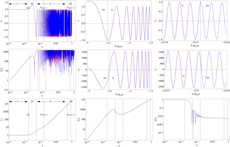
Figure 13: Analytic approximations compared to numerical solutions for $k=1$ $h$ ${\rm Mpc}^{-1}$. This comparison serves as a check for regions I, IV, V and VI. The red dotted line corresponds to the analytic solution and the blue to the numerical one.

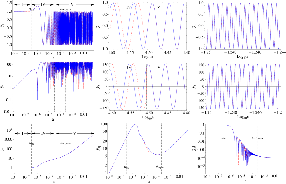
Figure 14: Analytic approximations compared to numerical solutions for $k=10$ $h$ ${\rm Mpc}^{-1}$. The colour scheme is the same as that in figure 13. Due to the large number of oscillations, the numerical solution breaks down at around $a\sim 0.2$ and thus the mode traverses regions I, IV, V.

We now compare the analytic forms given above with a numerical solution to the Boltzmann system. The numerical solution to eqs. 5a, 5b, 5c, 5d and 5e was generated using an implicit Runge-Kutta solver inbuilt in the software package ‘Mathematica’ (Wolfram Research, 2008). The solution was evolved from $a_{i}=10^{-8}$ to $a_{f}=1$ with initial conditions given by eqs. 6a, 6b, 6c and 6d. The value of $y_{5,i}$ was $0.01$. We considered three cases $k=5\times 10^{-5},1$ and $10$ $h$ ${\rm Mpc}^{-1}$. The figures below plot the scaled variable

$${\tilde{y}_{n}}=\frac{y_{n}}{y_{n,i}},$$ (57)

where $y_{n}$, $n=1\ldots 5$ is the variable of interest and $y_{n,i}$ is its initial value.

Figures 12 shows the evolution of the mode $k=5\times 10^{-5}$ $h$ ${\rm Mpc}^{-1}$ from $a=10^{-8}$ to $a=1$. This mode stays outside the horizon throughout its evolution until today and provides a check for the evolution in regions I, II and III. To construct the analytic solution initial conditions are needed at the starting epoch of each region. The initial conditions for region I are the same as those that the numerical solution is started with. To define the initial conditions for the other regions, the numerical solution is read off at two epochs: $a(\Omega_{r}=0.9)$ i.e., end of radiation domination and $a(\Omega_{r}=0.001)$ i.e., beginning of the matter-dark energy era. This provides initial conditions for regions II and III respectively. It can be seen from figure 12 that the agreement between the analytic approximation and numerics is good.

Figure 13 shows the evolution of the mode $k=1$ $h$ ${\rm Mpc}^{-1}$. This mode crosses the horizon during the radiation domination era. Thus it starts in region I and covers regions IV, V and VI as it evolves. Here too the initial conditions for region I are those that the numerical solution started with. The interface between region I and IV is the epoch when the mode crosses the horizon denoted as $a_{hc}$. The numerical solution is read off at $a_{hc}$, at $a(\Omega_{r}=0.9)$ and at $a(\Omega_{r}=0.001)$ to provide initial conditions for regions IV, V and VI respectively. The agreement between the analytic answer and numerical solution is good. The first two rows of plots show the radiation variables $y_{1}$ and $y_{2}$. In each of these rows, the middle (right) plot shows a blown up interval around the transition between region IV (V) and region V (VI). Note that the approximation in region V worsens with time. This is because in constructing the radiation solutions in region V, we used the adiabatic approximation to obtain the coefficients $a_{3}$ and $b_{4}$ in eq. (54). This construction assumes that the parameter $\Omega_{m}$ is constant over the interval of integration. Although the time derivative of $\Omega_{m}$ is small, it is non-zero and the breakdown of this approximation causes the two solutions to deviate. For region VI, the initial conditions for the analytic approximations read-off from the numerical solutions; thus by construction the two solutions match at the junction between regions V and VI. The last row shows $y_{3},y_{4}$ and $y_{5}$. Note that $y_{5}$ includes is constructed by using eq. (16) and includes the contribution from the radiation variables. Thus we are able to reproduce the oscillations in $y_{5}$ to some extent.

Figure 14 shows the evolution of the mode $k=10$ $h$ ${\rm Mpc}^{-1}$. This mode crosses the horizon during the radiation domination era, but the oscillations in the radiation variables are too large to allow evolution up until $a=1$ and the mode is evolved only until $a=0.27$. Thus it passes through regions I, IV and V. The initial conditions are set in a similar fashion to the $k=1$ mode. Note that the solution gets worse in region IV: this signals the breakdown of the radiation domination region. The natural question to ask is why this breakdown is not as prominent in the $k=1$ ${\rm Mpc}^{-1}$ case ? The reason is because in constructing the solutions, the starting point is to express $y_{5}$ only in terms of $y_{1}$ and $y_{2}$ through eq. (16); the $\Omega_{m}y_{3}$ and $\Omega_{m}y_{4}$ terms in this expression are ignored. When the radiation domination approximation breaks down the $\Omega_{m}$ term cannot be neglected, but it is weighted by $y_{3}$ and $y_{4}$. These are higher for higher values of $k$; thus the breakdown of the approximation occurs earlier for these values.

9 Conclusions

In this paper, we have investigated the mathematical properties of the E-B system using an eigenvalue analysis and computed analytical solutions in six different regimes of evolution. The main focus of our work was the dark matter power spectrum and hence it sufficed to consider a reduced set of variables. Thus, the photons are characterised only by their monopole and dipole moments $\Theta_{0}$ and $\Theta_{1}$ and dark matter is characterised by its density $\rho$ and irrotational peculiar velocity $v$ in the Newtonian gauge. The photon and matter sectors are indirectly coupled via the gravitational potential $\Phi$ and their dynamics is dictated by the linearized E-B system. For mathematical simplicity, baryons and neutrinos were excluded from the system. Traditional analyses evolve the E-B system as a function of the conformal time $\eta$. Instead we chose the time variable as $\ln a$ and further simplified the system by making a change of coordinates. This allowed us to clearly define three parameters that dictate the evolution: the matter and radiation density parameters $\Omega_{m}$ and $\Omega_{r}$ and a parameter $\epsilon=k/(Ha)$, which is the ratio of the Hubble time to the oscillation time of a photon mode. These parameters are time-dependent, making this system non-autonomous, but we have defined appropriate ‘adiabatic conditions’ when the parameters vary ‘slowly’ and the system can be considered‘quasi-autonomous’.

The results from the investigation of the E-B system can be summarized in two parts. In the first part we perform an eigenvalue analysis which gives insight into various interesting properties of the system.

1. Onset of oscillations: There are five eigenvalues for the system, which depend on $\epsilon$, $\Omega_{m}$ and $\Omega_{r}$. For every mode the eigenvalues transition from being all real (four negative and one positive) to three real (two negative, one positive) and two complex (with negative real parts). The appearance of complex eigenvalues denotes the presence of oscillations. By applying Sturm’s theorem and Decartes rule of sign, were able to analytically predict the transition epoch. We find that this epoch differs for each $k$; for a larger $k$ the transition occurs earlier. For $k\gtrsim 0.1$ $h$ ${\rm Mpc}^{-1}$, the transition occurs just after horizon crossing whereas for $k\lesssim 0.1$ $h$ ${\rm Mpc}^{-1}$, it occurs well before horizon crossing. We know from the analytical solutions and from the magnitude of the imaginary eigenvalue that the frequency of oscillations is of order $\epsilon$. This means that the oscillations are never visible for the super-horizon modes and that the high-frequency oscillations in sub-horizon modes occur well after the mode has crossed the horizon.

2. Stability of a numerical solver: We analyzed the stability properties of two classes of numerical schemes, namely, general Runge-Kutta methods and linear multistep methods. The stability of these schemes applied to a eigenvalue problem ${\dot{y}}=\lambda y$ is governed by the step size and eigenvalue. Applying the stability condition allowed us to estimate the step size given the eigenvalue. Typically, this condition imposes a maximum bound on the step size for explicit schemes and a minimum bound for implicit schemes.

3. Stiffness: In the literature, the ‘stiffness’ of the E-B system is often attributed to the presence of baryons because the time scales of Thomson scattering are much smaller than the Hubble time. We demonstrated that the late time regime of rapid oscillations also corresponds to the presence of two widely separated time scales making the system stiff. These rapid oscillations are present even in the absence of baryons. To better characterise stiffness, we plot the stiffness parameter defined as the ratio of the most and least negative eigenvalues (including eigenvalues with negative real parts) and find that this ratio is large for almost all modes and epochs of interest.

In the second part, we provide analytic solutions in six asymptotic regions of the $k-a$ plane which are defined in terms of the values of $\Omega_{m}$, $\Omega_{r}$ and $\epsilon$. Most of these limits have been discussed individually by various authors, primarily solving for the potential $\Phi$. Here we provide a comprehensive list of solutions for all five variables and give them explicitly in terms of the initial conditions. This allows an independent comparison in each region of the $k-a$ plane. The solutions for sub-horizon modes are constructed using the ‘adiabatic condition’. However, this condition is not satisfied by all sub-horizon modes. Thus there is a range $k=0.1-0.0001$ $h$ ${\rm Mpc}^{-1}$ where solution for all five variables can be constructed only until the modes are super-horizon. We compared the analytic solutions for $k=5\times 10^{-5},1,10$ $h$ ${\rm Mpc}^{-1}$ with the numerical solutions and found a good match. Figure 11 summarizes our results for the different mathematical regimes of the system and the applicability of the asymptotic analytical solutions.

In this paper, we considered a restricted set of variables; those that influence the broad features of the dark matter power spectrum. The full system includes baryons and neutrinos and possibly other interacting species. New interactions will introduce new time scales in the problem. These may imply additional adiabatic conditions and it is conceivable that the system may not be adiabatic with respect to all parameters at the same time. Defining them appropriately will depend upon the problem at hand. Adiabaticity is an important criterion to satisfy because the stability analysis for autonomous systems is relatively simple. For non-autonomous system, using eigenvalues to analyze stability (of the system itself) or the numerical solver can sometimes give inaccurate results. The full system also consists of the whole hierarchy of multipoles resulting in a large number of perturbation variables. Numerically, computing the eigenvalues of the linear operator may be computationally intensive and cumbersome. In this work we have considered the equations only in the conformal Newtonian gauge; the equations could be recast in synchronous gauge or in terms of gauge independent variables. All these extensions potentially complicate the analysis, but the framework and results presented in this paper can still be applied to gain some insight into the mathematical structure of the system and thus help facilitate further code development and testing.

10 Acknowledgements

SN would like to acknowledge the Science and Engineering Research Board (SERB) for the grant (YSS/2014/000526) and would like to thank Sayantani Bhattacharyya and Sagar Chakraborty for useful discussions. AR would like to thank Adam Amara and Lukas Gamper for useful discussions. In addition, AR thanks the Tata Institute for Fundamental Research, where part of this work was done, for its hospitality and adjunct faculty programme support. We would like to thank Julien Lesgourgues and Antony Lewis for useful comments on the manuscript.

Appendix A Useful identities

The three parameters are

$$\epsilon=\frac{k}{Ha},\Omega_{m}=\frac{\Omega_{m,0}H_{0}^{2}a_{0}^{3}}{H^{2}a^{3}}\;\;{\rm and}\;\;\Omega_{r}=\frac{\Omega_{m,0}H_{0}^{2}a_{0}^{4}}{H^{2}a^{4}},$$ (58)

where

$$H^{2}=H_{0}^{2}\left[\frac{\Omega_{m,0}a_{0}^{3}}{a^{3}}+\frac{\Omega_{r,0}a_{0}^{4}}{a^{4}}+\Omega_{\Lambda,0}\right].$$ (59)

Hence,

$$2H\frac{dH}{da}=\frac{H_{0}^{2}}{a}\left[-3\frac{\Omega_{m,0}a_{0}^{3}}{a^{3}}-4\frac{\Omega_{r,0}a_{0}^{4}}{a^{4}}\right].$$ (60)

Using the definitions of $\Omega_{m}$ and $\Omega_{r}$ gives

$$\frac{d\ln H}{d\ln a}=-\frac{1}{2}(3\Omega_{m}+4\Omega_{r}).$$ (61)

Differentiating $\epsilon$,

$$\frac{d\epsilon}{da}=-\frac{k}{a^{2}H}\left[1+\frac{a}{H}\frac{dH}{da}\right].$$ (62)

Substituting for the definition of $\epsilon$ and the derivative of $H$, gives

$$\frac{d\ln\epsilon}{d\ln a}=-\left[1-\frac{1}{2}(3\Omega_{m}+4\Omega_{r})\right].$$ (63)

Differentiating $\Omega_{m}$,

$$\frac{d\Omega_{m}}{da}=-\frac{\Omega_{m,0}a_{0}^{3}}{a^{3}H^{2}}\left[\frac{3}{a}+\frac{2}{H}\frac{dH}{da}\right]$$ (64)

which, upon substituting for $dH/da$ and using the definition of $\Omega_{m}$ gives

$$\frac{d\ln\Omega_{m}}{d\ln a}=-[3-(3\Omega_{m}+4\Omega_{r})].$$ (65)

Similarly, the derivative for $\Omega_{r}$ is

$$\frac{d\ln\Omega_{r}}{d\ln a}=-[4-(3\Omega_{m}+4\Omega_{r})].$$ (66)

Appendix B Sturm’s theorem

The characteristic polynomial of the Jacobian matrix ${\mathcal{A}}$ has five real roots a early epochs and three real roots at later epochs. The transition between these two structures denotes the onset of oscillations. Although the eigenvalues are not known analytically, it is possible to compute the number of real roots using Sturm’s theorem and Descartes’ rule of sign described below.

Sturm’s theorem (Collins & Akritas, 1976; Hook & McAree, 1990) gives the number of distinct real roots of a polynomial $p(x)$ in an interval $(a,b)$ by counting the number of changes of signs of the Sturm’s sequence at the end points of the interval. Given a $n$-th order polynomial $p(x)$, the Sturm sequence is constructed as follows:

$$p_{0}(x) = p(x)$$ (67)

$$p_{1}(x) = p^{\prime}(x)$$ (68)

$$p_{2}(x) = -{\rm Rem}[p_{0}(x),p_{1}(x)]$$ (69)

$$p_{3}(x) = -{\rm Rem}[p_{1}(x),p_{2}(x)]$$ (70)

$$\vdots$$ (71)

$$0 = -{\rm Rem}[p_{n-1}(x),p_{n}(x)],$$ (72)

where ${\rm Rem}[p_{i}(x),p_{i+1}(x)]$ is the remainder of the polynomial division $p_{i}x)/p_{i+1}(x)$. The degree of each polynomial in the chain successively decreases and this sequence usually culminates in a constant. The minimum number of divisions is always less than or equal to the degree of the polynomial. The signs of each of these polynomials are recorded at the two end points, $a$ and $b$, in ascending order of the degree of the polynomial and the number of sign changes are noted at each end. Let this be $n_{a}$ and $n_{b}$ respectively. The number of real roots is then $|n_{a}-n_{b}|$.

Using Sturm’s theorem on the characteristic polynomial of ${\mathcal{A}}$, we first establish that there are two different root structures and the the transition point is evaluated by solving for the epoch at which the number of real roots changes from five (at early epochs) to three. The characteristic polynomial is

$$c_{5}\lambda^{5}+c_{4}\lambda^{4}+c_{3}\lambda^{3}+c_{2}\lambda^{2}+c_{1}\lambda+c_{0}=0,$$ (73)

where

$$c_{0} = \frac{\Omega_{m}\epsilon^{4}}{6}$$ (74)

$$c_{1} = -\frac{1}{18}\epsilon^{2}\left[9\Omega_{m}+2(3-6\Omega_{r}+\epsilon^{2})\right]$$ (75)

$$c_{2} = -\frac{1}{9}\epsilon^{2}\left[6-6\Omega_{r}+\epsilon^{2}\right]$$ (76)

$$c_{3} = -\frac{1}{6}\left[6+9\Omega_{m}+12\Omega_{r}+4\epsilon^{2}\right]$$ (77)

$$c_{4} = -\frac{1}{6}\left[9\Omega_{m}+2(6+6\Omega_{r}+\epsilon^{2})\right]$$ (78)

$$c_{5} = -1$$ (79)

The interval (a,b) in this case corresponds to $(-\infty,+\infty)$. This polynomial has five roots. Applying Sturm’s theorem we find that there are two different root structures: at sufficiently early epochs, all roots are real; eventually, two complex roots are generated and three roots are real. The transition epoch depends upon $k$ and $a$ and is denoted as $a_{trans}(k,a)$. Sturm’s theorem does not indicate the sign of the roots. The signs of the real roots can be estimated using Descartes’ rule of sign. The rule states the following. Consider a single-variable polynomial ordered by descending variable exponents. Let $n$ be the number of sign changes between consecutive non-zero coefficients. Then the number of positive roots is equal to $n$ or less than $n$ by an even number. Similarly, the upper bound on the number of negative roots can be estimated by multiplying the coefficients of odd powers by minus one. Applying Descartes’ rule of sign to our case, we note that the coefficients $c_{2},c_{3},c_{4},c_{5}$ are always negative and $c_{0}$ is always positive. $c_{1}$ can be either positive or negative. This gives the constraint that the number of positive roots is less than or equal to one. In estimating the negative roots we change the signs of $c_{1},c_{3}$ and $c_{5}$. Hence $c_{3},c_{5}$ are always positive while $c_{2},c_{4}$ are always negative for all epochs. $c_{1}$ changes sign, but in either cases, the rule gives four or two or zero negative roots at all times. We note that Descartes’ rule of sign does not give the absolute number of real roots; just an upper bound. Combining with Sturm’s theorem, we infer that when all five roots are real, one must be positive and four negative and when three are real, two have to be negative (all three cannot be negative by the rule of signs) and one has to be positive.

In principle, to obtain the transition epoch analytically, one must compute the Sturm sequence, evaluate it at $(-\infty,+\infty)$ and find the sign changes. But this is a cumbersome task. Instead we can guess the transition epoch from the rule of signs. Since $c_{1}$ is the only term in the coefficients that changes sign during the evolution, it is plausible that the transition epoch corresponds to the transition of the sign of this term. Thus, we postulate that the transition epoch satisfies the relation

$$(9\Omega_{m}(a_{trans})+2(3-6\Omega_{r}(a_{trans})+\epsilon(a_{trans},k)^{2}))=0.$$ (80)

We find that the analytical predictions of the transition epoch using the Descartes’ rule of sign match the numerical prediction using Sturm’s theorem.

Appendix C Frequency of oscillations

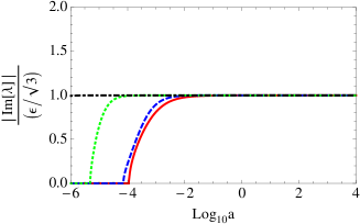
Figure 15: Ratio of the imaginary part of the eigenvalue to $\epsilon(k,a)$. The colour coding is same as that of figure 2. It is clear that at late times the imaginary part which determines the ‘instantaneous’ frequency is proportional to $\epsilon$. We found that this figure does not change even when $\Omega_{\Lambda}$ is set to zero.

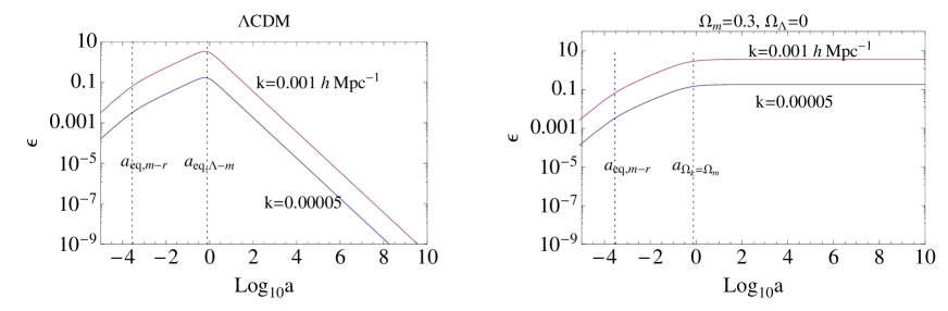
Figure 16: The variation of $\epsilon$ for the $\Lambda$CDM cosmology and another open model with the same $\Omega_{m}$ and $\Omega_{r}$ as the $\Lambda$CDM model, but with $\Omega_{Lambda}=0$. For both models $k_{eq,m-r}$ = In the former case, $\epsilon$ stays small throughout the evolution for $k\ll k_{eq}$.

As is discussed in §5, Sturm’s theorem predicts the transition to oscillations, by identifying the epoch when the eigenvalues of the system become imaginary. This transition epoch depends explicitly on $\Omega_{m}$ and $\Omega_{r}$ but not on $\Omega_{\Lambda}$. The $\Omega_{\Lambda}$ dependence is only through $\epsilon$. For small values $k<<k_{eq,m-r}$, the epoch occurs just before matter-radiation equality. However, as can be seen in figure 12, oscillations are not observed. This can be explained as follows. Sturm’s theorem predicts the transition to complex eigenvalues but not their magnitude. Numerically, we find that the imaginary part of the eigenvalue which determines the ‘instantaneous’ frequency of oscillations is proportional to $\epsilon$ at late times (see figure 15).

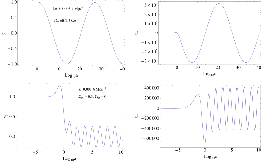
Figure 17: Extended evolution for a cosmology with the same $\Omega_{m}$ and $\Omega_{r}$ as the $\Lambda$CDM case, but with $\Omega_{\Lambda}=0$. Oscillations are seen for long enough evolution times.

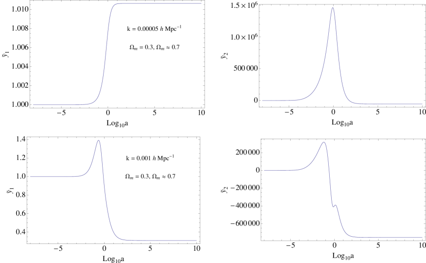
Figure 18: Extended evolution for the $\Lambda$CDM cosmology. The ‘instantaneous’ frequency is too small for noticeable oscillations.

In the $\Lambda$CDM cosmology, $\epsilon$ starts small, reaches a maximum at $a=1$ and drops very sharply after the epoch of dark energy-matter equality $a_{eq,\Lambda-m}$ (see the left panel of figure 16). For small values of $k$ ($k\ll k_{eq,m-r}$), $\epsilon$ stays small throughout the evolution. For example $k=5\times 10^{-5}$ $h$ ${\rm Mpc}^{-1}$, $\epsilon\sim 0.1$ at $a\sim 1$ and drops thereafter. Thus, no oscillations are visible because the oscillation frequency is very small. In roughly 8 e-folds (from $a\sim a_{eq,m-r}$ to $a\sim 1$) one expects to see around $8\times Im[\lambda]$ oscillations. For $Im[\lambda]\sim 0.5\epsilon$ and $\epsilon\sim 0.1$ this corresponds to about half a oscillation. To understand this issue better we contrast it with another cosmology with the same $\Omega_{m}$ and $\Omega_{r}$ as $\Lambda$CDM but $\Omega_{\Lambda}=0$. These two cosmologies have practically the same $k_{eq,m-r}$ and Sturm’s theorem predicts similar transition epochs. However, the $\epsilon$ variation is different. In the latter, $\epsilon$ tends to a constant because the curvature dominates (see right panel of figure 16). Thus, oscillations are seen for long enough evolution times. This is illustrated in figures 17 (open cosmology with $\Omega_{\Lambda}=0$) and 18 ($\Lambda$CDM). In each figure, the two rows correspond to two different values of $k$; each row shows the evolution of $y_{1}$ and $y_{2}$ for extended evolution times. Oscillations are clearly visible in the open cosmology. The oscillation frequency is higher for a higher value of $k$ since $\epsilon$ is higher . Figure 18 shows that, for the $\Lambda$CDM case, oscillations cannot be sustained. We note that the oscillations in the system are primarily in the $y_{1}$ and $y_{2}$ (radiation) sector: since $\Omega_{r}$ is small after the transition epoch, these variables couple very weakly to the potential $y_{5}$ and there are no oscillations visible in the matter sector. Also, from a practical perspective, there are no visible oscillations before $a=1$ in any of the cases: again this is because the oscillation frequency is small in this domain.

Appendix D Stability of numerical schemes

Consider the general differential equation

$$\frac{dy}{dx}=f(x,y[x]),$$ (81)

with a given initial condition $y[x_{0}]=y_{0}$. If $f(x,y[x])\equiv f(y[x])$, i.e., $f$ has no explicit time dependence, then the dynamical system is autonomous, else is it a non-autonomous system. To solve the equation numerically, the domain is discretized into finite number of grid points $\{x_{0},x_{1},\ldots\}$. The separation between the grid points gives the step size $h_{n}=x_{n}-x_{n-1}$. The values of the function at any point are given by $y({x_{n}})=y_{n}$ and the derivatives are denoted as $f_{n}$. The simplest numerical scheme to solve this system is the explicit (or forward) Euler’s method. In this scheme,

$$y_{n}=y_{n-1}+hf_{n-1},\;\;\;n=1,2\ldots$$ (82)

Although computationally simple, this scheme is not very stable and there are various extensions possible: (a) perform more number of computations (stages) within a step (RK schemes), (b) keep higher order derivatives in the Taylor expansion (Taylor series solutions), (c) use more past values in computing $y_{n}$ (multistep scheme) (d) use higher order derivatives of $f$ (Rosenbrock methods). See Butcher (1987), section 214, for a nice schematic diagram showing these extensions. In this paper, we will consider (a) general RK schemes and (c) linear multistep schemes.

D.1 Runge-Kutta (RK) schemes

The commonly used 4th-order RK scheme is of the form

$$y_{n} =y_{n-1}+h\left(\frac{1}{6}k_{1}+\frac{1}{3}k_{2}+\frac{1}{3}k_{3}+\frac{1}{6}k_{4}\right),$$ (83a)

$${\rm where}\;\;k_{1} =f(x_{n-1},y_{n-1})$$ (83b)

$$k_{2} =f(x_{n-1}+\frac{h}{2},y_{n-1}+\frac{h}{2}k_{1})$$ (83c)

$$k_{3} =f(x_{n-1}+\frac{h}{2},y_{n-1}+\frac{h}{2}k_{2})$$ (83d)

$$k_{4} =f(x_{n-1}+h,y_{n-1}+hk_{3}).$$ (83e)

The forms listed above are explicit in the sense that the step at $y_{n}$ can be computed completely from the knowledge of the function at all points upto $y_{n-1}$. This scheme has four stages and it can be shown that the error between the numerical solution after $n$ steps ($y_{n}$) and the exact solution at the position of the $n$-th step ($y_{exact}[x_{n}])$) scales as ${\mathcal{O}}(h^{4})$ (hence fourth order). This is an explicit scheme because the solution for the function after $n$ steps $y_{n}$ depends only on the solution at earlier time steps. A general explicit RK scheme with $s$ stages has the form:

$$y_{n}=y_{n-1}+h\sum_{i=1}^{s}b_{i}k_{i},$$ (84)

where

$$k_{i}=f(x_{n-1}+c_{i}h,y_{n-1}+h\sum_{j<i}a_{ij}k_{j}).$$ (85)

Thus, the method is completely characterised by the matrix $a_{ij}$ (called the Runge-Kutta matrix), the numbers $b_{i}$ (called the weights) and the numbers $c_{i}$ (called the nodes). This is usually represented in the form of a table called the Butcher tableau.

$$\begin{array}[]{c|ccccc}0&0&0&0&\cdots&0\\ c_{2}&a_{21}&0&0&\cdots&0\\ c_{3}&a_{31}&a_{32}&0&\cdots&0\\ \vdots&\vdots&\vdots&\ddots&\cdots&0\\ c_{2}&a_{s1}&a_{s2}&\cdots&a_{ss-1}&0\\ \hline\cr&b_{1}&b_{2}&b_{3}&\cdots&b_{s}\end{array}\equiv\begin{array}[]{c|c}{\bf c}&{\bf A}\\ \hline\cr&{\bf b^{T}}\end{array}$$ (86)

The Butcher tableau of the forward Euler scheme is

$$\begin{array}[]{c|c}0&0\\ \hline\cr&1\end{array}$$ (87)

The Butcher tableau of the fourth-order RK integration is

$$\begin{array}[]{c|cccc}0&0&0&0&0\\ \frac{1}{2}&\frac{1}{2}&0&0&0\\ \frac{1}{2}&0&\frac{1}{2}&0&0\\ 1&0&0&1&0\\ \hline\cr&\frac{1}{6}&\frac{1}{3}&\frac{1}{3}&\frac{1}{6}\end{array}$$ (88)

D.1.1 Implicit Methods

Explicit schemes are simple to implement, but often unstable and implicit schemes need to be employed. An implicit method usually involves solving a functional equation for $y_{n}$ at each time step. Although they are generally computationally intensive implicit schemes are generally more stable.

The backward Euler scheme has the form

$$y_{n}=y_{n-1}+hf(x_{n},y_{n}).$$ (89)

and a general implicit RK method has the form

$$y_{n}=y_{n-1}+h\sum_{i=1}^{s}b_{i}k_{i},$$ (90)

where

$$k_{i}=f(x_{n-1}+c_{i}h,y_{n-1}+h\sum_{j=i}^{s}a_{ij}k_{j}).$$ (91)

Note that the sum is not restricted to $j<i$ as was in the explicit case. Thus, the matrix $A$ in the Butcher tableau is no longer a lower triangular matrix and in general all entries are non-zero. The Butcher tableau for a implicit (backward) Euler scheme is

$$\begin{array}[]{c|c}1&1\\ \hline\cr&1\end{array}$$ (92)

and for the implicit mid-point scheme given by

$$y_{1}=y_{0}+hf(x_{0}+\frac{h}{2},y_{0}+\frac{h}{2}k_{1})$$ (93)

it is

$$\begin{array}[]{c|c}1/2&1/2\\ \hline\cr&1\end{array}$$ (94)

D.1.2 Stability of a RK scheme

The stability of a numerical scheme is loosely defined as its ability to reproduce the qualitative behaviour of the exact analytic solution. For example, if the analytic solution converges to zero, it is expected that the numerical solution does the same. Consider the solution to the one-dimensional linear autonomous differential equation

$$\frac{dy}{dx}=\lambda y.$$ (95)

If $x_{0}$ is the starting point, the exact analytic solution at the $n+1$-th step is

$$y(x_{0}+nh)=e^{\lambda nh}y(x_{0}).$$ (96)

The exact analytic solution is bounded if and only if $|e^{\lambda h}|\leq 1$, which is equivalent to ${\mathcal{R}e}(\lambda h)\leq 0$. Since $h$ is always positive, this is equivalent to stating that the solution is bounded if and only if ${\mathcal{R}e}(\lambda)\leq 0$. Consider the numerical solution for the same system using the explicit Euler scheme. After the $n$-th step, the approximate solution is

$$y_{n}=(1+h\lambda)^{n}y_{0}.$$ (97)

For the numerical solution, the boundedness condition translates to $|1+\lambda h|\leq 1$. Thus, given the eigenvalue, this condition gives a minimum step size. The function $r(z)=1+z$ where $z=\lambda h$ is the stability function of the forward Euler scheme. For a multi-dimensional system ${\dot{\bf y}}={\mathcal{H}}{\bf y}$, we can assume without loss of generality that ${\mathcal{H}}$ is diagonal and perform the analysis in the eigenbasis (Butcher, 1987). The limits on the step size can be converted to limits on step sizes in a different basis using the basis transformation.

For a general RK scheme applied to autonomous differential equations, the stability function is (Butcher 1987; Harrier & Wanner 1996)

$$r(z)=1+zb^{T}(I-zA)^{-1}e=\frac{\det(I-zA+zeb^{T})}{\det(I-zA)},$$ (98)

where, $z=\lambda h$, $e=\{1,1,1,\ldots\}^{T}$ is a s-dimensional vector and $b^{T},A$ are to be read off from the Butcher tableau of the method. The stability condition is given by

$$|r(z)|\leq 1.$$ (99)

The stability functions for some commonly used RK methods are given in table 2 in the text. The stability function for explicit methods is always a polynomial whereas for implicit methods it is always a ratio of rational functions of $z$. A more exhaustive list for implicit methods can be found in Harrier & Wanner (1996), page 42. To compute the allowed step size $h$, one has to solve the equation $|r(z=h\lambda)|=1$.

D.1.3 Non-Autonomous systems

For a linear non-autonomous system, the stability function is generalized. For each stage at the $n$-th step of a RK method, define

$$z_{i} = h\lambda(x_{n-1}+hc_{i})$$ (100)

$$Z = {\rm diag}(z_{1},z_{2},\ldots z_{s})$$ (101)

$$R(Z) = 1+b^{T}Z(1-AZ)^{-1}e.$$ (102)

A RK method applied to a non-autonomous system is stable if, for all $z_{1},z_{2},\ldots,z_{s}$, such that $det(I-AZ)\neq 0$,

$$|R(Z)|\leq 1.$$ (103)

When the system is autonomous, all $z_{i}$ are identical and $r(z)=R(zI)$, where $I$ is the identity matrix. For the Euler scheme, there is only one stage so $Z=z$ and $R(z)=r(z)$. The conditions to be solved for stability are

1. Explicit Euler scheme

   $$|R(h,x)|=|1+h\lambda(x+h)|=1$$ (104)

2. Implicit Euler scheme

   $$|R(h,x)|=\left|\frac{1}{1-h\lambda(x+h)}\right|=1.$$ (105)

3. Implicit midpoint scheme

   $$|R(h,x)|=\left|\frac{2+h\lambda(x+h/2)}{2-h\lambda(x+h/2)}\right|=1$$ (106)

4. Explicit RK-4

   $$R(h,x)=1+\frac{z_{1}}{6}+\frac{z_{2}}{3}+\frac{z_{3}}{3}+\frac{z_{4}}{6}+\frac{z_{1}z_{2}}{6}+\frac{z_{2}z_{3}}{6}+\frac{z_{3}z_{4}}{6}+\frac{z_{1}z_{2}z_{3}}{12}+\frac{z_{2}z_{3}z_{4}}{12}+\frac{z_{1}z_{2}z_{3}z_{4}}{24},$$ (107)

   where the $z_{i}$s are functions of the eigenvalues evaluated at the sub-grid points defined by the nodes ($c_{i}$ values in the Butcher tableau):

   $$z_{1} = h\lambda(x)$$ (108)

   $$z_{2} = h\lambda(x+\frac{h}{2})$$ (109)

   $$z_{3} = h\lambda(x+\frac{h}{2})$$ (110)

   $$z_{4} = h\lambda(x+h).$$ (111)

Thus, to solve for the step size along each eigendirection, one has to solve $|R(h,x)|=1$ at each point in the domain for the corresponding eigenvalue.

D.2 Linear multistep methods

Another important family of methods are the linear multistep methods. Here the $n$-th step can depend upon previous steps. There are two sub-families of these methods: Adams methods and Backward Differentiation Formula (BDF) methods.

1. Adams method: The $k$-step explicit Adams method (also called Adams-Bashforth methods) is of the form

   $$y_{n}=y_{n-1}+h\sum_{j=1}^{k}\beta_{i}f_{n-j},$$ (112)

   where

   $$\beta_{j} = (-1)^{j-1}\sum_{i=j-1}^{k-1}\binom{l}{j-1}\gamma_{l}$$

   $$\gamma_{l} = (-1)^{l}\int_{0}^{1}\binom{-s}{l}ds$$

   The forward Euler method given by eq. (82) corresponds to a Adams-Bashforth method with $k=1$ and $\beta=1$. The $k$-step implicit Adams method (also called Adams-Moulton) method has the form

   $$y_{n}=y_{n-1}+h\sum_{j=0}^{k}\beta_{i}f_{n-j},$$ (113)

   The backward Euler method given by eq. (89) corresponds to $k=1$ and $\beta_{1}=1$. The implicit trapezoidal rule given by

   $$y_{n}=y_{n-1}+\frac{h}{2}(f_{n}+f_{n-1})$$ (114)

   corresponds to $k=1$ with $\beta_{0}=\beta_{1}=\frac{1}{2}$.

2. Backward Differentiation Formula (BDF) method: A $k$-step BDF method is given by

   $$\alpha_{0}y_{n}+\alpha_{1}y_{n-1}+\ldots+\alpha_{k}y_{n-k}=h\beta_{0}f_{n},$$ (115)

   where $\alpha_{i}$s and $\beta_{0}$ are derived by requiring that the error scale with a given order (order conditions). BDF1 is a first order method with $\alpha_{0}=1$, $\alpha_{1}=-1$ and $\beta_{0}=1$ and corresponds to the backward Euler scheme. BDF2 is a second order method which gives

   $$y_{n}=\frac{4}{3}y_{n-1}-\frac{1}{3}y_{n-2}+\frac{2}{3}hf_{n}.$$ (116)

Note that ‘linear’ here refers to the method; in general, $f(y_{n})$ could be a non-linear function of $y_{n}$.

D.2.1 Stability

A general linear $k$-step method has the general form (Petzold & Ascher, 1998)

$$\alpha_{0}y_{n}+\alpha_{1}y_{n-1}+\alpha_{2}y_{n-2}+\ldots=h(\beta_{0}f_{n}+\beta_{1}f_{n-1}+\beta_{2}f_{n-2}+\ldots).$$ (117)

The choice $\alpha_{0}=1$ sets the overall scaling. For all Adams methods, $\alpha_{j}=0$ for $j>1$ and for all BDF methods, $\beta_{j}=0$ for $j>0$. Suppose $f_{n}=f(y_{n})=\lambda y_{n}$; i.e., $\lambda$ is the eigenvalue of the 1D problem ${\dot{y}}=\lambda y$. This form then becomes

$$\sum_{k=0}^{j}(\alpha_{j}-h\lambda\beta_{j})y_{n-j}=0.$$ (118)

This is a homogenous constant coefficient difference equation whose solutions can be expanded in terms of the roots $\xi_{i}$ of the polynomial

$$\phi(\xi)=\sum_{k=0}^{j}\alpha_{j}\xi^{n-j}-h\lambda\sum_{k=0}^{j}\beta_{j}\xi^{n-j}.$$ (119)

Usually the first sum is denoted as $\rho(\xi)$ and the second as $\sigma(\xi)$ so that $\phi(\xi)=\rho(\xi)-h\lambda\sigma(\xi)$. From the theory of difference equations, the solutions are stable if and only if the roots of the equation $\phi(\xi)=0$ satisfy

$$|\xi_{root}(z)|\leq 1\;\;\;{\rm for\;all\;roots},$$ (120)

where $z=\lambda h$. They are absolutely stable if and only if $|\xi_{root}(z)|<1$. The stability polynomials for some methods are computed below. The stability is dictated by the behaviour in the complex $z$ plane.

1. Forward Euler ($k=1$ explicit Adams) has $\alpha_{0}=1,\beta_{0}=0,\alpha_{1}=-1,\beta_{1}=1$. The stability polynomial is

   $$\phi(\xi)=1-(1+z)\xi^{-1},$$ (121)

   whose root is

   $$\xi_{root}(z)=1+z.$$ (122)

2. Backward Euler ($k=1$ implicit Adams, first order or BDF1) has $\alpha_{0}=1,\beta_{0}=1,\alpha_{1}=-1,\beta_{1}=0$. The stability polynomial is

   $$\phi(\xi)=(1-z)-\xi^{-1},$$ (123)

   whose root is

   $$\xi_{root}(z)=\frac{1}{(1-z)}.$$ (124)

3. Trapezoidal Rule ($k=1$ implicit Adams, second order) has $\alpha_{0}=1,\beta_{0}=1/2,\alpha_{1}=-1,\beta_{1}=1/2$. The characteristic polynomial becomes

   $$\phi(\xi)=(1-\frac{z}{2})+(-1-\frac{z}{2})\xi^{-1},$$ (125)

   whose root is

   $$\xi_{root}(z)=\frac{2+z}{2-z}$$ (126)

4. BDF2 scheme has $\alpha_{0}=1,\alpha_{1}=-\frac{4}{3},\alpha_{2}=\frac{1}{3},\beta_{0}=\frac{2}{3}$. The stability polynomial becomes

   $$\phi(\xi)=\left(1-\frac{2z}{3}\right)-\frac{4}{3}\frac{1}{\xi}+\frac{1}{3\xi^{2}},$$ (127)

   whose roots are

   $$\xi_{root}(z)=\frac{2\pm\sqrt{1+2z}}{3-2z}.$$ (128)

   The condition $|\xi_{root}|\leq 1$ corresponding to root with the negative sign gives stability for all $z$. Thus, the constraining condition is given by the root corresponding to the positive sign.

5. BDF3 scheme has $\alpha_{0}=1,\alpha_{1}=-\frac{18}{11},\alpha_{2}=\frac{9}{11},\alpha_{3}=-\frac{2}{11},\beta_{0}=\frac{6}{11}$. The stability polynomial becomes

   $$\phi(\xi)=(11-6z)\xi^{3}-18\xi^{2}+9\xi+2.$$ (129)

   There are three roots. Numerically, we find that the complex roots always satisfy the stability condition. The constraining condition is given by the real root:

   $$\xi_{root}(z)=\frac{6}{11-6z}+\frac{27-162z}{9(11-6z)f(z)}+\frac{f(z)}{11-6z},$$ (130)

   where $f(z)=(40+30z+36z^{2}+\sqrt{1573+1914z+864z^{2}-3672z^{3}+1296z^{4}})^{1/3}$. In the text we use the notation $r(z)=\xi_{root}(z)$ to denote the stability function.

Figure 6 in the text shows the regions of stability in the complex $z$ plane for some popular methods. Generally, implicit methods are more stable than explicit methods. For the backward Euler and the BDF2 and 3 schemes, the stability criterion sets a lower bound on the step size for a positive eigenvalue. For example with a BDF2 scheme, $h_{min}=4/\lambda$. A smaller step size will imply instability. For the BDF schemes, the size of the domain where the scheme is unstable increases with order. Thus, a higher order BDF scheme will converge faster, but the step size will have a greater restriction. A trade-off between stability and efficiency may be required while employing such schemes.

Appendix E Detailed derivations of analytic forms in various limits

The system to solve is given by eq. (5) given arbitrary initial conditions $y_{1,i}$ to $y_{5,i}$. We consider two limits: $\epsilon\ll 1$ giving the super-horizon solutions and $\epsilon\gtrsim 1$ giving the sub-horizon solutions. Within each class we consider three epochs: radiation domination, when $\Omega_{r}\gg\Omega_{m}$, matter-radiation era when $\Omega_{m}$ and $\Omega_{r}$ are both non-zero and dark energy-matter era, when $\Omega_{r}\ll 1$. This defines six separate regions where analytic forms can be obtained.

E.1 Super-horizon modes: $\epsilon\ll 1$

In the limit that $\epsilon\ll 1$, neglecting all terms of order $\epsilon$ or higher, gives

$${\dot{y}}_{1}=0;\;\;{\dot{y}}_{2}=0;\;\;{\dot{y}}_{3}=0;\;\;{\dot{y}}_{4}=-y_{4}\;\;$$ (131)

and

$${\dot{y}}_{5}=\frac{1}{2}\left[\Omega_{m}y_{3}+4\Omega_{r}y_{1}-(3\Omega_{m}+4\Omega_{r}+2)y_{5}\right].$$ (132)

The solutions to the first four variables are

$$y_{1}=y_{1,i};\;\;y_{2}=y_{2,i};\;\;y_{3}=y_{3,i};\;\;y_{4}=\frac{y_{4,i}a_{i}}{a}.$$ (133)

Substituting for $y_{1}$ and $y_{3}$ in eq. (132) gives

$${\dot{y}}_{5}=\frac{1}{2}\left[\Omega_{m}y_{3,i}+4\Omega_{r}y_{1,i}-(3\Omega_{m}+4\Omega_{r}+2)y_{5}\right].$$ (134)

E.1.1 Regions I and II: super-horizon modes in the radiation domination and radiation-matter eras

The solutions for both these regions can be obtained simultaneously. We solve eq. (134) using an integrating factor $s$ defined as

$${\dot{s}}=s\frac{3\Omega_{m}+4\Omega_{r}+2}{2}.$$ (135)

In terms of this factor eq. (134) becomes

$$\frac{d(y_{5}\cdot s)}{d\ln a}=\frac{\Omega_{m}y_{3,i}+4\Omega_{r}y_{1,i}}{2}\cdot s.$$ (136)

The solution is

$$y_{5}s=\int_{a_{i}}^{a}s\cdot\left(\frac{\Omega_{m}y_{3,i}+4\Omega_{r}y_{1,i}}{2}\right)d\ln a+c,$$ (137)

with $c=y_{5,i}s_{i}$ where $s_{i}=s(a_{i})$. To proceed further, one must solve for the integrating factor. From eq. (135) the solution for $s$ is

$$\ln s(a)=\int\left(\frac{3\Omega_{m}+4\Omega_{r}+2}{2}\right)d\ln a$$ (138)

Using the derivative of $\Omega_{m}$ from eq. (10) the integrand can be written as

$$\frac{3\Omega_{m}+4\Omega_{r}+2}{2}=\frac{1}{2}\frac{d\ln\Omega_{m}}{d\ln a}+\frac{5}{2}.$$ (139)

This gives

$$s(a)=\Omega_{m}^{1/2}a^{1/2}.$$ (140)

Substituting for $s$ in eq. (137) gives

$$a^{5/2}\Omega_{m}^{1/2}y_{5}=\int_{a_{i}}^{a}a^{5/2}\Omega_{m}^{1/2}\cdot\left(\frac{\Omega_{m}y_{3,i}+4\Omega_{r}y_{1,i}}{2}\right)d\ln a+y_{5,i}\Omega_{m,i}^{1/2}a_{i}^{5/2}.$$ (141)

Now, define

$$x=\frac{a}{a_{eq,m-r}},$$ (142)

where $a_{eq,m-r}=\frac{\Omega_{r,0}}{\Omega_{m,0}}$. In the radiation-matter regime,

$$H^{2}=H_{0}^{2}(\Omega_{m,0}a^{-3}+\Omega_{r,0}a^{-4}),$$ (143)

and using eq. (7), the parameters in terms of $x$ are

$$\Omega_{r}=\frac{1}{1+x};\;\;\;\Omega_{m}=\frac{x}{1+x}.$$ (144)

In terms of $x$ eq. (141) becomes

$$\frac{x^{3}}{\sqrt{1+x}}\cdot y_{5} = \int_{x_{i}}^{x}\frac{x^{3}}{\sqrt{1+x}}\left(\frac{y_{3,i}}{2}\frac{x}{1+x}+\frac{2y_{1,i}}{1+x}\right)d\ln x+\frac{y_{5,i}x_{i}^{3}}{\sqrt{1+x_{i}}}$$ (145)

$$= \frac{y_{3,i}}{2}\int_{x_{i}}^{x}\frac{x^{3}}{(1+x)^{3/2}}dx+2y_{1,i}\int_{x_{i}}^{x}\frac{x^{2}}{(1+x)^{3/2}}dx+\frac{y_{5,i}x_{i}^{3}}{\sqrt{1+x_{i}}}$$ (146)

$$= \frac{y_{3,i}}{5}\left.\left\{\frac{16+8x-2x^{2}+x^{3}}{\sqrt{1+x}}\right\}\right|_{x,i}^{x}+\frac{4y_{1,i}}{3}\left.\left\{\frac{-8-4x+x^{2}}{\sqrt{1+x}}\right\}\right|_{x,i}^{x}+\frac{y_{5,i}x_{i}^{3}}{\sqrt{1+x_{i}}}$$ (147)

Thus, the full solution is

$$y_{5}(x)=\frac{\sqrt{1+x}}{x^{3}}\left(\frac{y_{3,i}}{5}\left.\left\{\frac{16+8x-2x^{2}+x^{3}}{\sqrt{1+x}}\right\}\right|_{x,i}^{x}+\frac{4y_{1,i}}{3}\left.\left\{\frac{-8-4x+x^{2}}{\sqrt{1+x}}\right\}\right|_{x,i}^{x}\right)+y_{5,i}\left(\frac{x_{i}}{x}\right)^{3}\sqrt{\frac{1+x}{1+x_{i}}}$$ (148)

This solution is true for any initial conditions $y_{5,i}$, $y_{3,i}$ and $y_{1,i}$ (can, in principle, be specified independently).
Approximations
When $x_{i}\ll 1$, the last term can be ignored and the terms in the curly brackets evaluated at $x_{i}$ reduce to just constants. Thus, the solution is

$$y_{5}(x)\approx\frac{\sqrt{1+x}}{x^{3}}\left(\frac{-16y_{3,i}}{5}+\frac{32y_{1,i}}{3}\right)+\frac{y_{3,i}}{5}\left(\frac{16+8x-2x^{2}+x^{3}}{x^{3}}\right)+\frac{4y_{1,i}}{3}\left(\frac{-8-4x+x^{2}}{x^{3}}\right)$$ (149)

Further, when $y_{3,i}=9/2y_{5,i}$ and $y_{1,i}=3/2y_{5,i}$ as given by the adiabatic initial conditions (see eq. (6)), the solution becomes

$$y_{5}(x)\approx\frac{y_{5,i}}{10}\left(\frac{16\sqrt{1+x}}{x^{3}}-\frac{16}{x^{3}}-\frac{8}{x^{2}}+\frac{2}{x}+9\right).$$ (150)

This agrees with the solution obtained by Kodama & Sasaki (1984). Note that eqs. (148), eq. (149) and (150) give the right limit at the initial time: when $x\ll 1$, $y_{5}(x\ll 1)\approx y_{5,i}$.

E.1.2 Region III: super-horizon modes in the matter-dark energy era

In this limit, $\Omega_{r}\approx 0$ and eq. (134) becomes

$${\dot{y}}_{5}=\left[\Omega_{m}y_{3}-(3\Omega_{m}+2)y_{5}\right].$$ (151)

Change the dependent variable from $a$ to $\Omega_{m}$ using eq. (10). This gives

$${\dot{y}}_{5}=\frac{dy_{5}}{d\Omega_{m}}\cdot 3\Omega_{m}(\Omega_{m}-1),$$ (152)

and eq. (151) becomes

$$\frac{dy_{5}}{d\Omega_{m}}+\frac{y_{3,i}}{6(1-\Omega_{m})}-\frac{(3\Omega_{m}+2)}{\Omega_{m}(1-\Omega_{m})}y_{5}=0.$$ (153)

The solution to this equation is in terms of hypergeometric functions.

$$y_{5}(\Omega_{m})=\frac{C\Omega_{m}^{1/3}}{(1-\Omega_{m})^{5/6}}-\frac{y_{3,i}}{4}\frac{\Omega_{m}}{(1-\Omega_{m})^{5/6}}\;\;{}_{2}F_{1}\left(\frac{2}{3},\frac{1}{6},\frac{5}{3},\Omega_{m}\right),$$ (154)

where the hypergeometric function (or series) is given by (Arfken 2000, 4^th edition)

$${}_{2}F_{1}(a,b,c,x)=\sum_{n=0}^{\infty}\frac{(a)_{n}(b)_{n}}{(c)_{n}}\frac{x^{n}}{n!},$$ (155)

$${\rm with}\;\;(a)_{n}=a(a+1)(a+2)\ldots(a+n-1)=\frac{(a+n-1)!}{(a-1)!}\;\;{\rm and}\;(a)_{0}=1.$$ (156)

It is possible to recast the solution in terms of the variable $x$ defined as

$$x=\frac{a}{a_{eq,\Lambda-m}},$$ (157)

where

$$a_{eq,\Lambda-m}=\left(\frac{\Omega_{m,0}}{\Omega_{\Lambda,0}}\right)^{1/3}.$$ (158)

This gives $\Omega_{m}=(1+x^{3})^{-1}$ and the solution becomes

$$y_{5}(x)=C\frac{\sqrt{1+x^{3}}}{x^{5/2}}-\frac{y_{3,i}}{4}\frac{1}{x^{5/2}(1+x^{3})^{1/6}}\;\;{}_{2}F_{1}\left(\frac{2}{3},\frac{1}{6},\frac{5}{3},\frac{1}{1+x^{3}}\right).$$ (159)

The first term in the above expression is the homogenous solution and the second is the particular solution. Here $C$ is set by the initial conditions. $C=y_{5,i}\frac{x_{i}^{5/2}}{\sqrt{1+x_{i}^{3}}}+\frac{y_{3,i}}{4}\frac{1}{(1+x_{i}^{3})^{2/3}}\;\;{}_{2}F_{1}\left(\frac{2}{3},\frac{1}{6},\frac{5}{3},\frac{1}{1+x_{i}^{3}}\right)$. When $x_{i}\ll 1$, $C\rightarrow\frac{y_{3,i}}{4}\;\;{}_{2}F_{1}\left(\frac{2}{3},\frac{1}{6},\frac{5}{3},1\right)$. The solutions above were obtained by ignoring the $\epsilon$ terms in the equations. It is possible to obtained refined approximations for $y_{1}$ to $y_{4}$ by substituting the above solutions in eqs. 5a, 5b, 5c and 5d and integrating the resulting equations. This gives

$$y_{1}(k,a) =y_{1,i}-y_{2,i}\int_{a_{i}}^{a}\frac{\epsilon(k,a)}{3}d\ln a$$ (160a)

$$y_{2}(k,a) =y_{2,i}+y_{1,i}\int_{a_{i}}^{a}\epsilon(k,a)d\ln a-2\int_{a_{i}}^{a}y_{5}(a)\epsilon(k,a)d\ln a$$ (160b)

$$y_{3}(k,a) =y_{3,i}-y_{4,i}a_{i}\int_{a_{i}}^{a}\frac{\epsilon(k,a)}{a}d\ln a,$$ (160c)

where $y_{5}(a)=y_{5}(x=a/a_{eq,m-r})$ given above. Deep in the radiation dominated era, $\epsilon\sim a$ and $y_{5}(a)\sim y_{5,i}$ and the solution is $y_{2}(k,a)\sim y_{2,i}+(y_{1,i}-2y_{5,i})(\epsilon(k,a)-\epsilon(k,a_{i}))$. In the other regimes, the integral is computed numerically. Consider eq. (5d) for $y_{4}$. This can be re-written as

$$\frac{d(ay_{4})}{da}=-\epsilon(k,a)y_{5}(a).$$ (161)

Integrating once gives,

$$y_{4}(k,a)=\frac{y_{4,i}a_{i}}{a}-\frac{1}{a}\int_{a_{i}}^{a}\epsilon(k,a)y_{5}(a)da.$$ (162)

In the radiation dominated era, the integral can be computed easily giving $y_{4}(k,a)\sim\frac{y_{4,i}a_{i}}{a}-y_{5,i}\frac{\epsilon}{2a^{2}}(a^{2}-a_{i}^{2})$; for other regions we compute it numerically.

E.2 Horizon crossing ($\epsilon\sim 1$) and sub-horizon modes ($\epsilon>1$).

To track the evolution of modes through horizon crossing and soon after, we need to solve the system eqs. 5a to 5e for non-zero $\epsilon$. The radiation and matter variables are coupled through $y_{5}$. In the radiation domination era, the coupled $y_{1},y_{2}$ and $y_{5}$ system is solved first and the resulting $y_{5}$ sources the matter variables $y_{3}$ and $y_{4}$. In the radiation-matter and matter-dark energy eras the coupled $y_{3},y_{4}$ and $y_{5}$ system is solved first and the resulting $y_{5}$ sources the radiation variables $y_{1}$ and $y_{2}$.

E.2.1 Region IV: sub-horizon modes in the radiation domination era

The three equations that govern $y_{1},y_{2}$ and $y_{3}$ are eqs. (5a), (5b) and eq. (5e). In addition, the algebraic equation for $y_{5}$ in the radiation domination regime becomes

$$y_{5}=\frac{4}{B_{rad}}\left(y_{1}+\frac{1}{\epsilon}y_{2}\right),$$ (163)

where $B_{rad}=4+2\epsilon^{2}/3$ and we have additionally assumed $\Omega_{r}\approx 1$ and $\Omega_{m}\approx 0$. As explained in the text, using the algebraic form for $y_{5}$ as a solution is justified for initial conditions set by inflation. Thus, there remain two degrees of freedom and we derive a second order differential equation for $y_{5}$ as follows.

In the radiation domination limit, eq. (5e) becomes.

$${\dot{y}}_{5}=2y_{1}-\frac{B_{rad}+2}{2}y_{5},$$ (164)

Differentiate w.r.t. $\ln a$ and substitute eq. (5a) to get

$${\ddot{y}}_{5}=-\frac{2\epsilon}{3}y_{2}-\left(\frac{B_{rad}+2}{2}\right){\dot{y}_{5}}-\frac{{\dot{B}}_{rad}}{2}y_{5}.$$ (165)

Eliminate $y_{1}$ from eqs. (163) and (164) to express $y_{2}$ as

$$y_{2}=-\frac{\epsilon}{2}(y_{5}+{\dot{y}}_{5}).$$ (166)

Substitute for $y_{2}$ in eq. (164) to get

$${\ddot{y}}_{5}={\dot{y}}_{5}\left(\frac{\epsilon^{2}}{3}-\frac{B_{rad}+2}{2}\right)+y_{5}\left(\frac{\epsilon^{2}}{3}-\frac{{\dot{B}_{rad}}}{2}\right).$$ (167)

Now in the radiation era,

$${\dot{B}}_{rad}\approx 4\epsilon{\dot{\epsilon}}/3\;\;\;{\rm and\;from\;eq.(\ref{epsder})}\;\;\;{\dot{\epsilon}}=\epsilon\implies{\dot{B}}_{rad}=4\epsilon^{2}/3$$ (168)

Substituting for $B_{rad}$ and ${\dot{B}}_{rad}$ above gives

$${\ddot{y}}_{5}+3{\dot{y}}_{5}+\frac{\epsilon^{2}}{3}y_{5}=0.$$ (169)

Since $\epsilon\sim a$ in the radiation era,

$$\frac{d}{d\ln a}=\epsilon\frac{d}{d\epsilon}\;\;\;\;{\rm and}\;\;\;\frac{d^{2}}{d\ln a^{2}}=\epsilon\frac{d}{d\epsilon}+\epsilon^{2}\frac{d^{2}}{d\epsilon^{2}}$$ (170)

Thus in terms of $\epsilon$, the equation for $y_{5}$ in the radiation era is

$$\epsilon^{2}\frac{d^{2}y_{5}}{d\epsilon^{2}}+4\epsilon\frac{dy_{5}}{d\epsilon}+\frac{\epsilon^{2}}{3}y_{5}=0.$$ (171)

Define two new variables: the independent variable $x=\epsilon/\sqrt{3}$ and the dependent variable $u=y_{5}x$. Substituting in eq. (171) gives the equation for $u$ and denoting derivatives w.r.t. $x$ with primes we get

$$x^{2}u^{\prime\prime}+2xu^{\prime}+(x^{2}-2)u=0,$$ (172)

whose solution is

$$u(x)=a_{1}J_{1}(x)+a_{2}N_{1}(x),$$ (173)

where $J_{1}(x)$ and $N_{1}(x)$ are the Spherical Bessel functions of the first and second kind (the latter also called the spherical Neumann function). Thus, in the radiation limit when $\epsilon\gtrsim 1$, the solution for $y_{5}$ is

$$y_{5}(x)=a_{1}\left(\frac{\sin x-x\cos x}{x^{3}}\right)-a_{2}\left(\frac{x\sin x+\cos x}{x^{3}}\right).$$ (174)

To compute $y_{2}$, use eq. (166) and convert the dots (derivative w.r.t. $\ln a$) to primes (derivative w.r.t. $x$) to give

$$y_{2}=-\frac{\sqrt{3}x}{2}\left(y_{5}(x)+xy_{5}^{\prime}(x)\right).$$ (175)

Substituting from eq. (174) gives

$$y_{2}(x)=-\frac{\sqrt{3}}{2x^{2}}\left[\left\{2a_{2}x+a_{1}\left(x^{2}-2\right)\right\}\sin x+\left\{2a_{1}x-a_{2}\left(x^{2}-2\right)\right\}\cos x\right].$$ (176)

Using eq. (5b) and converting to $x$ variables gives

$$y_{1}=\frac{1}{\sqrt{3}}y_{2}^{\prime}(a)+2y_{5}(x).$$ (177)

Substituting for $y_{2}$ from eq. (176) gives

$$y_{1}(x)=-\frac{1}{2x}\left[(a_{2}x-2a_{1})\sin x+(a_{1}x+2a_{2})\cos x\right].$$ (178)

Once $y_{5}$ is known, the matter fields can be determined. Differentiating eq. (5c) and substituting from eq. (5d) gives the equation

$${\ddot{y}}_{3}+\left(1-\frac{{\dot{\epsilon}}}{\epsilon}\right){\dot{y}}_{3}-\epsilon^{2}y_{5}=0.$$ (179)

In the radiation dominated limit, ${\dot{\epsilon}}/{\epsilon}\approx 1$ and the equation becomes

$${\ddot{y}}_{3}=\epsilon^{2}y_{5}.$$ (180)

Integrating once gives

$${\dot{y}_{3}}=\int_{a_{i}}^{a}\epsilon^{2}y_{5}d\ln a+c.$$ (181)

Converting to the $x$ variable ($\epsilon=\sqrt{3}x$ and $d\ln a=d\ln x$ in the radiation dominated era) gives

$${\dot{y}_{3}}(x)=\frac{dy_{3}}{d\ln x}=\int_{x_{i}}^{x}3xy_{5}(x)dx+c=\frac{3}{xx_{i}}\left[a_{1}(x\sin x_{i}-x_{i}\sin x)+a_{2}(x_{i}\cos x-x\cos x_{i})\right]+c,$$ (182)

where $c$ is the integration constant $c={\dot{y}}_{3,i}=-\sqrt{3}x_{i}y_{4,i}$. This is

Using eq. (5c) $y_{4}$ can be written in the $x$ variable as

$$y_{4}(x)=-\frac{1}{\sqrt{3}x}{\dot{y}}_{3}.$$ (183)

Substituting from eq. (182) gives

$$y_{4}(x)=-\frac{\sqrt{3}}{x^{2}x_{i}}\left[a_{1}(x\sin x_{i}-x_{i}\sin x)+a_{2}(x_{i}\cos x-x\cos x_{i})\right]+\frac{y_{4,i}x_{i}}{x}.$$ (184)

Integrating eq. (182) once more gives $y_{3}=\int_{a_{i}}^{a}{\dot{y}}_{3}d\ln a=\int_{x_{i}}^{x}\frac{dy_{3}}{d\ln x}d\ln x$. Using eq. (182) gives

$$y_{3}(x)=3a_{1}\left.\left(\frac{\sin x}{x}+\ln x\frac{\sin x_{i}}{x_{i}}-\text{Ci}(x)\right)\right|_{x_{i}}^{x}-3a_{2}\left.\left(\frac{\cos x}{x}+\ln x\frac{\cos x_{i}}{x_{i}}+\text{Si}(x)\right)\right|_{x_{i}}^{x}-\sqrt{3}y_{4,i}x_{i}(\ln x-\ln x_{i})+y_{3,i},$$ (185)

where

$$\text{Ci}(x)=-\int_{x}^{\infty}\frac{\cos x^{\prime}}{x^{\prime}}dx^{\prime}\;\;\;{\rm and}\;\;\;\text{Si}(x)=\int_{0}^{x}\frac{\sin x^{\prime}}{x^{\prime}}dx^{\prime}.$$ (186)

$a_{1}$ and $a_{2}$ have to be set from initial conditions. There are two ways to set these constants. One choice is use the initial conditions $y_{1,i}$ and $y_{2,i}$ and solve $a_{1}$ and $a_{2}$. The other choice is to demand that $y_{5}$ is a constant at very early epochs, when $\epsilon\ll 1$. In this limit, $a_{2}=0$ and $a_{1}=3y_{5,i}$. Note that for $\epsilon\ll 1$, this choice gives $y_{1,i}\approx 3/2y_{5,i}$ and $y_{2,i}\approx-\epsilon_{i}/2y_{5,i}$.

Solutions of the E-B ystem in this regime have been derived analytically by Hu & Sugiyama (1996). They obtain a logarithmic growth for the matter overdensity $\delta$. This logarithmic growth is also reflected in our solution for $y_{3}$ (which is equal to $\delta+3\Phi$). The solutions derived above are valid for all $\epsilon$ in the radiation dominated era. No approximations made in the derivation invoke the magnitude of $\epsilon$. Thus, the solutions are also valid when $\epsilon\ll 1$ and are expected to reduce to the super-horizon solutions for $x\ll 1$.

E.2.2 Region V: sub-horizon modes in the radiation-matter era

Here we first solve for the coupled system $y_{3},y_{4}$ and $y_{5}$ and use the resulting solution to solve for the radiation variables. The three main equations are eqs. (5c), (5d) and (5e). These three are combined with the algebraic equation eq. (16) to give a second order system. There are two main approximations made in this regime: (1) Although, $\Omega_{r}$ is not set to zero, perturbations in the radiation sector are ignored, and (2) $\epsilon$ is large enough such that $2\epsilon^{2}/3\gg 3\Omega_{m}+4\Omega_{r}$.

The starting point is eq. (179) which is valid at all epochs and scales (because it was derived directly from eqs. (5c) and (5d)). We wish to express $y_{5}$ in terms of $y_{3}$ and its derivatives so that one can obtain a second order differential variable in $y_{3}$. This is done by combining eqs. (16), where the radiation perturbations are ignored with eq. (5c). Ignoring the radiation perturbations, eq. (16) becomes

$$y_{5}=\frac{1}{B}\left[\Omega_{m}\left(y_{3}+\frac{3y_{4}}{\epsilon}\right)\right].$$ (187)

Eliminate $y_{4}$ from the above by using eq. (5c) to give $y_{5}$ in terms of $y_{3}$ and ${\dot{y}}_{3}$. Substitute the resulting $y_{5}$ in eq. (179) to give a second order equation for $y_{3}$:

$${\ddot{y}}_{3}+\left(1-\frac{\dot{\epsilon}}{\epsilon}+\frac{3\Omega_{m}}{B}\right){\dot{y}}_{3}-\frac{\Omega_{m}}{B}y_{3}\epsilon^{2}=0.$$ (188)

Now, in the matter dominated eras, for most typical scales of interest, $\epsilon\gtrsim 1$ and hence the $\epsilon^{2}$ term dominates in the expression for $B$. Note that this approximation is not valid in the radiation dominated era. Setting $B\sim 2\epsilon^{2}/3$, gives

$${\ddot{y}}_{3}+\left(1-\frac{\dot{\epsilon}}{\epsilon}\right){\dot{y}}_{3}-\frac{3\Omega_{m}}{2}y_{3}=0,$$ (189)

$$\implies {\ddot{y}}_{3}+\left(2-\frac{3\Omega_{m}}{2}-2\Omega_{r}\right){\dot{y}}_{3}-\frac{3}{2}\Omega_{m}y_{3}=0,$$ (190)

where in the second equation is obtained by substituting for for ${\dot{\epsilon}}$ from eq. (9). There is no $k$-dependence of $y_{3}$ in this regime and the only parameters in the equation are $\Omega_{m}$ and $\Omega_{r}$. This allows us to introduce the variable

$$x=\frac{a}{a_{eq,m-r}},$$ (191)

as defined in eq. (142). Using eq. (144) to substitute for the $\Omega$s, we get

$$y^{\prime\prime}_{3}+\frac{3x+2}{2x(1+x)}y^{\prime}_{3}-\frac{3}{2}\frac{y_{3}}{x(1+x)}=0,$$ (192)

where the primes denote derivatives w.r.t. $x$. In the matter dominated era, when $x$ is large but before dark energy domination takes over, one mode grows as the scale factor i.e., linear in $x$. Thus, one solution has to be a polynomial of degree one in $x$ with $y^{\prime\prime}(x)=0$. This solution satisfies

$$\frac{y^{\prime}_{3}}{y_{3}}=\frac{3}{3x+2},$$ (193)

whose solution is

$$y^{(1st)}_{3}=3x+2.$$ (194)

The superscript denotes the ‘first’ solution. For a homogenous equation like the one above, the second solution can be constructed if one is known (Arfken (2000), page 501). The second solution is

$$y^{(2nd)}_{3} = (3x+2)\int\frac{\exp\left\{-\int\frac{3x^{\prime}+2}{2x^{\prime}(1+x^{\prime})}dx^{\prime}\right\}}{(3x+2)^{2}}dx$$ (195)

$$= (3x+2)\int\frac{dx}{x\sqrt{1+x}(3x+2)^{2}}$$ (196)

$$= -\frac{3}{4}\left[\left(x+\frac{2}{3}\right)\log\left(\frac{\sqrt{1+x}+1}{\sqrt{1+x}-1}\right)-2\sqrt{1+x}\right],$$ (197)

where the integral was performed with the transformation $u=\sqrt{1+x}$. Thus, the general solution is

$$y_{3}=c_{3}\left(x+\frac{2}{3}\right)+c_{4}\left[\left(x+\frac{2}{3}\right)\log\left(\frac{\sqrt{1+x}+1}{\sqrt{1+x}-1}\right)-2\sqrt{1+x}\right],$$ (198)

and using $y_{4}=-\epsilon^{-1}xy^{\prime}_{3}$ gives

$$y_{4}=-\frac{1}{\epsilon(k,a_{eq}x)}\left\{c_{3}x+c_{4}\left[x\log\left(\frac{\sqrt{1+x}+1}{\sqrt{1+x}-1}\right)-\frac{2(1+3x)}{3\sqrt{1+x}}\right]\right\}.$$ (199)

The constants $c_{1}$ and $c_{2}$ can be set either by the initial conditions of $y_{3}$ and $y_{4}$ or by matching to the logarithmic solution for small scale modes in the radiation era.

At first glance, it may seem inconsistent to keep the $\Omega_{r}$ in writing ${\dot{\epsilon}}$, but ignore the $\Omega_{r}$ term in eq. (187). Suppose this term is kept and the full expression for $y_{5}$ is substituted in eq. (179). The term $\epsilon^{2}y_{5}$ appearing in that equation then has a contribution $\Omega_{r}y_{1}$ (assuming $B\sim\epsilon^{2}$). But note that, in the radiation dominated era, the solution for $y_{1}$ decays as $1/\epsilon$ (see eq. (178)). Thus, the contribution of the $\Omega_{r}y_{1}$ term is of $\mathcal{O}(\epsilon^{-1})$, whereas in ${\dot{\epsilon}}/\epsilon$ the $\Omega_{r}$ term is of $\mathcal{O}(1)$. Since, we have assumed $\epsilon\gg 1$ ignoring the former is justified. This point has also been discussed in a detailed footnote in Weinberg (2002).

Having computed $y_{3}$ and $y_{4}$, $y_{5}$ follows from eq. (187). $y_{5}$ is a source term for the coupled radiation system. To compute these solutions we will use the adiabatic approximation. First note that the radiation sector, for all values of $\epsilon$, can re-written in terms of two other variables

$$\dot{w} = \frac{i\epsilon}{\sqrt{3}}w-\frac{2i\epsilon}{\sqrt{3}}y_{5}$$ (200)

$$\dot{v} = -\frac{i\epsilon}{\sqrt{3}}v+\frac{2i\epsilon}{\sqrt{3}}y_{5},$$ (201)

where

$$w = y_{1}+\frac{i}{\sqrt{3}}y_{2}$$ (202)

$$v = y_{1}-\frac{i}{\sqrt{3}}y_{2}.$$ (203)

The homogenous solutions for $w$ and $v$ and hence also for $y_{1}$ and $y_{2}$ are combinations of $\cos I(k,a)$ and $\sin I(k,a)$ where

$$I(k,a)=\int_{a_{i}}^{a}\frac{\epsilon(k,a^{\prime})}{\sqrt{3}}d\ln a^{\prime}.$$ (204)

The $y_{5}$ term decides the particular solution for this system and eq. (187) gives $y_{5}$ in terms of $y_{3}$ and $y_{4}$. We invoke the adiabatic approximation to assume that in the radiation-matter regime when $\epsilon\gg 1$, the parameters $\Omega_{m}$ and $\Omega_{r}$ are approximately constants (see §4). For the particular solution, we assume the ansatz:

$$y_{p,1}(a) = a_{3}y_{3}(a)+a_{4}y_{4}(a),$$ (205)

$$y_{p,2}(a) = b_{3}y_{3}(a)+b_{4}y_{4}(a),$$ (206)

where $a_{3},a_{4}$ are constants. Substitute this ansatz in eqs. (5a) and (5b) and use eqs. (5c), (5d) and eq. (187) to solve for $a_{3},b_{3},a_{4}$ and $b_{4}$. This gives

$$a_{3}=\frac{2\Omega_{m}}{B+3\Omega_{m}},\;\;a_{4}=0,\;\;b_{3}=0,\;\;b_{4}=\frac{6\Omega_{m}}{B+3\Omega_{m}}.$$ (207)

Thus,

$$y_{1}(a) = c_{1}\cos I(k,a)+c_{2}\sin I(k,a)+a_{3}y_{3}(a)$$ (208)

$$y_{2}(a) = \sqrt{3}\left(c_{1}\sin I(k,a)-c_{2}\cos I(k,a)\right)+b_{4}y_{4}(k,a)$$ (209)

Putting the initial conditions that $y_{1}(a_{i})=y_{1,i}$ and ${\dot{y}_{1}}(a_{i})=3y_{2,i}/\epsilon_{i}$ gives

$$c_{1}=y_{1,i}-a_{3}y_{3,i}\;\;\;c_{2}=-\frac{1}{\sqrt{3}}(y_{2,i}-b_{4}y_{4,i})$$ (210)

Note that the adiabatic approximation was not invoked in solving for the matter variables. Thus, having computed $y_{1}$, $y_{2}$, $y_{3}$ and $y_{4}$ is it possible to get a refined estimate of $y_{5}$ using eq. (16). This is more accurate than eq. (187). Some of the above solutions have been worked out in the past by Meszaros (1974); Hu & Sugiyama (1996); Weinberg (2002).

E.2.3 Region VI: sub-horizon modes in the matter-dark energy era

In this regime, $\Omega_{r}\approx 0$, but there is a possible dark energy component. Here we consider it to be the cosmological constant. In this case ${\dot{\epsilon}}=-\epsilon(1-3\Omega_{m}/2)$ and eq. (188) becomes

$${\ddot{y}}_{3}+\left(2-\frac{3}{2}\Omega_{m}\right){\dot{y}}_{3}-\frac{3}{2}\Omega_{m}y_{3}=0.$$ (211)

Using eqs. (61) and (10),

$${\dot{H}} = -\frac{3\Omega_{m}H}{2},$$ (212)

$${\rm and}\;\;{\ddot{H}} = \frac{9}{2}H\Omega_{m}(1-\frac{\Omega_{m}}{2})$$ (213)

and it is easy to see that $y_{3}\sim H$ is one solution to the above equation. Thus, $y^{(1st)}\sim H$. Knowing the first solution, the second solution can be computed as

$$y_{3}^{(2nd)} = H\int\frac{\Omega_{m}^{1/2}}{a^{3/2}}H^{2}da.$$ (214)

$$\propto H\int\frac{da}{(aH)^{3}}.$$ (215)

Thus the full solution for $y_{3}$ is

$$y_{3}(a)=c_{3}H+c_{4}H\int\frac{da}{(aH)^{3}}.$$ (216)

From eq. (216), $y_{4}(a)$ becomes

$$y_{4}(a)=-\frac{1}{\epsilon}\left[c_{3}\frac{dH}{d\ln a}+c_{4}\left(\frac{1}{(aH)^{2}}+\frac{dH}{d\ln a}\int\frac{da}{(aH)^{3}}\right)\right].$$ (217)

$c_{3}$ and $c_{4}$ are set by the initial conditions $y_{3,i}$ and $y_{4i}$.
Recovering the usual linear growth equation: When $\Omega_{r}\approx 0$ and $\epsilon\gg 1$, eq. (187) becomes

$$y_{5}=\frac{\Omega_{m}}{B}y_{3},$$ (218)

where $B=3\Omega_{m}+\frac{2}{3}\epsilon^{2}$. Substituting the definition $y_{3}=\delta+3y_{5}$ gives

$$y_{5}\approx\frac{3\Omega_{m}\delta}{2}\;\;{\rm or}\;\;y_{3}\approx\delta.$$ (219)

Substituting $y_{5}$ in terms of $y_{3}$ in eq. (5e) and keeping terms to lowest order in $\epsilon$ gives ${\dot{y}}_{5}\approx 0$ or $y_{5}$ is a constant. With these limits, eqs. (5c) and (5d) become

$${\dot{\delta}} = -\epsilon y_{4}$$ (220)

$${\dot{y}}_{4} = -y_{4}-\frac{3}{2}\frac{\delta\Omega_{m}}{\epsilon}.$$ (221)

When these are combined we get

$${\ddot{\delta}}+\left(2-\frac{3}{2}\Omega_{m}\right){\dot{\delta}}-\frac{3\Omega_{m}}{2}\delta=0.$$ (222)

which is the usual linear growth equation. Note that the derivatives are w.r.t. $\ln a$ and $\Omega_{m}$ is the time-dependent matter density parameter (see eq. (7) in text).

E.3 Very small scales: $k\gtrsim 50$.

These modes have a very high value of $\epsilon$ even at very early times. We show that in this case, the radiation sector and matter sector can be decoupled. Each sector is solved separately and then combined to give the potential $y_{5}$.

We note that the solution for $y_{5}$ can be written as

$$y_{5}(k,a)=Cy_{5,hom}(k,a)+y_{5,part}(k,a),$$ (223)

where

$$y_{5,hom}(k,a) = \exp\left\{-\int_{a_{i}}^{a}\frac{B+2}{2}d\ln a\right\}$$

$$y_{5,part}(k,a) = \frac{1}{B}\left[4\Omega_{r}\left(y_{1}+\frac{1}{\epsilon}y_{2}\right)+\Omega_{m}\left(y_{3}+\frac{3}{\epsilon}y_{4}\right)\right]$$

$$C = y_{5,i}-y_{5,part}(a_{i}).$$

When $\epsilon$ is very large, the homogenous term in $y_{5}$ is exponentially suppressed and the particular solution is suppressed by $1/\epsilon^{2}$. Thus, the source terms in eqs. (200) and (201) are suppressed by $1/\epsilon$. Thus only the homogenous solutions remain which are

$$w(k,a) \approx w_{i}e^{iI(k,a)}$$ (224)

$$v(k,a) \approx v_{i}e^{-iI(k,a)},$$ (225)

where $I(k,a)$ is given by eq. (204). Converting back to the $y_{1},y_{2}$ variables gives

$$y_{1}(k,a) = y_{1,i}\cos I(k,a)-\frac{y_{2,i}}{\sqrt{3}}\sin I(k,a),$$ (226)

$$y_{2}(k,a) = y_{2,i}\cos I(k,a)+\sqrt{3}y_{1,i}\sin I(k,a).$$ (227)

In the matter sector, in eq. (5d), $y_{5}$ acts as a source term for $y_{4}$, which is also suppressed by $1/\epsilon$. Thus, only the homogenous term remains

$$y_{4}(a)=y_{4,i}\frac{a_{i}}{a}.$$ (228)

Integrating eq. (5c), gives

$$y_{3}(k,a)=y_{3,i}-\int_{a_{i}}^{a}\epsilon(k,a)y_{4}(k,a)d\ln a$$ (229)

In the radiation era, $\epsilon\sim a$. Substituting for $y_{4}$ from eq. (228) and

$$y_{3}(k,a)=y_{4,i}\frac{a_{i}}{a}\epsilon(k,a)\log\frac{a}{a_{i}}+y_{3,i}.$$ (230)

Substituting for $y_{1}$ to $y_{4}$ in eq. (223) gives, an estimate of $y_{5}$.

These arguments hold true only in the radiation dominated era since the radiation fields evolve as $1/\epsilon$ and the matter fields grow at best as $\ln a$. $\epsilon\sim a$ in this regime and the gravitational potential $y_{5}$ decays as $\ln a/a^{2}$ as can be seen from eq. (223). However, in the matter dominated era, $\epsilon\sim\sqrt{a}$ and $y_{3}\sim a$. So the gravitational potential $y_{5}$ does not decay, but instead goes to a constant $3\Omega_{m}y_{3}/(2\epsilon^{2})$ and the source terms involving $y_{5}$ in eqs. (200) and (201) actually grow as $\sqrt{a}$ and cannot be ignored.

Appendix F Including baryons and neutrinos

Here we recast the full system (including baryons and massless neutrinos) in terms of the variables defined in §2. The equations governing the perturbations in the cold dark matter, massless neutrinos, photons, baryons are given by equation 43, 50, 64 and 67 in Ma & Bertschinger (1995). We introduce the time variable ‘$\ln a$’; note that the derivative w.r.t. the conformal time $d/d\eta=aHd/d\ln a$. We also define three new parameters:

$$v = \frac{\theta}{k},$$ (231)

$$\epsilon_{k} = \frac{k}{aH},$$ (232)

$$\epsilon_{c} = \frac{an_{e}\sigma_{T}}{aH},$$ (233)

$$\epsilon_{H} = \frac{(aH)^{-1}}{\eta}.$$ (234)

Here $\epsilon_{k}$ is the same as the $\epsilon$ used elsewhere in the text. We use the subscript to distinguish it from $\epsilon_{c}$ and $\epsilon_{H}$. In terms of these parameters, the system is

$${\rm Cold}\;\;{\rm Dark}\;\;{\rm Matter}:\;\;\;\;\frac{d\delta_{c}}{d\ln a} =-\epsilon_{k}v_{c}+3\frac{d\phi}{d\ln a},$$ (235a)

$$\frac{dv_{c}}{d\ln a} =-v_{c}+\epsilon_{k}\psi$$ (235b)

$${\rm Massless}\;\;{\rm Neutrinos}:\;\;\;\;\frac{d\delta_{\nu}}{d\ln a} =-\frac{4}{3}\epsilon_{k}v_{\nu}+4\frac{d\phi}{d\ln a},$$ (235c)

$$\frac{dv_{\nu}}{d\ln a} =\epsilon_{k}\left(\frac{\delta_{\nu}}{4}-\sigma_{\nu}+\psi\right),$$ (235d)

$$\frac{dF_{\nu,l}}{d\ln a} =\frac{\epsilon_{k}}{2l+1}\left[lF_{\nu,l-1}-(l+1)F_{\nu,l+1}\right],$$ (235e)

$$\frac{dF_{\nu,l_{max}}}{d\ln a} =\epsilon_{k}F_{\nu,l_{max}-1}-\epsilon_{H}(l_{max}+1)F_{\nu,l_{max}}.$$ (235g)

$${\rm Photons}:\;\;\;\;\frac{d\delta_{\gamma}}{d\ln a} =-\frac{4}{3}\epsilon_{k}v_{\gamma}+4\frac{d\phi}{d\ln a},$$ (235h)

$$\frac{dv_{\gamma}}{d\ln a} =\epsilon_{k}\left(\frac{\delta_{\gamma}}{4}-\sigma_{\gamma}+\psi\right)+\epsilon_{c}(v_{b}-v_{\gamma}),$$ (235i)

$$\frac{dF_{\gamma 2}}{d\ln a} =\frac{8}{15}\epsilon_{k}v_{\gamma}-\frac{3}{5}\epsilon_{k}F_{\gamma,3}-\epsilon_{c}\left(\frac{9}{5}\sigma_{\gamma}-\frac{1}{10}(G_{\gamma 0}+G_{\gamma 2})\right),$$ (235j)

$$\frac{dF_{\gamma l}}{d\ln a} =\frac{\epsilon_{k}}{2l+1}\left[lF_{\gamma l-1}-(l+1)F_{\gamma l+1}\right]-\epsilon_{c}F_{\gamma l},$$ (235l)

$$\frac{dG_{\gamma l}}{d\ln a} =\frac{\epsilon_{k}}{2l+1}\left[lG_{\gamma l-1}-(l+1)G_{\gamma l+1}\right]-\epsilon_{c}\left[G_{\gamma l}-\frac{1}{2}\left(F_{\gamma 2}+G_{\gamma 0}+G_{\gamma 2}\right)\left(\delta_{l0}+\frac{\delta_{l2}}{5}\right)\right],$$ (235n)

$$\frac{dF_{\gamma l_{max}}}{d\ln a} =\epsilon_{k}F_{\gamma l_{max}-1}-\epsilon_{H}(l_{max}+1)F_{\gamma l_{max}}-\epsilon_{c}F_{\gamma l_{max}},$$ (235p)

$$\frac{dG_{\gamma l_{max}}}{d\ln a} =\epsilon_{k}G_{\gamma l_{max}-1}-\epsilon_{H}(l_{max}+1)G_{\gamma l_{max}}-\epsilon_{c}G_{\gamma l_{max}}.$$ (235r)

$${\rm Baryons}:\;\;\;\;\frac{d\delta_{b}}{d\ln a} =-\epsilon_{k}v_{b}+3\frac{d\phi}{d\ln a},$$ (235s)

$$\frac{dv_{b}}{d\ln a} =-v_{b}+\epsilon_{k}(c_{s}^{2}\delta_{b}+\psi)+\epsilon_{c}\frac{4\Omega_{\gamma}}{3\Omega_{b}}(v_{\gamma}-v_{b}).$$ (235t)

In this notation, the four coupled Einstein equations in the conformal Newtonian gauge become

$$\frac{d\phi}{d\ln a}+\psi+\frac{\epsilon_{k}^{2}}{3}\phi =-\frac{1}{2}\sum_{i}\Omega_{i}\delta_{i},$$ (236a)

$$\frac{d\phi}{d\ln a}+\psi =\frac{3}{2\epsilon_{k}}\sum_{i}\Omega_{i}(1+w_{i})v_{i},$$ (236b)

$$\frac{d^{2}\phi}{d\ln a^{2}}+\frac{d\phi}{d\ln a}\left(3+\frac{d\ln H}{d\ln a}\right)+\frac{d\psi}{d\ln a}+\left(3+2\frac{d\ln H}{d\ln a}\right)\psi+\frac{\epsilon_{k}^{2}}{3}(\phi-\psi) =\frac{3}{2}\sum_{i}w_{i}\delta_{i}\Omega_{i},$$ (236c)

$$\phi-\psi =\frac{9}{2\epsilon_{k}^{2}}\sum_{i}(1+w_{i})\Omega_{i}\sigma_{i}.$$ (236d)

Here sum over ‘$i$’ denotes sum over the various components. The tight coupling regime is when $\epsilon_{c}\gg 1$. When the photon moments oscillate rapidly, $\epsilon_{k}\gg 1$; this is also the regime when the photons are free-streaming and the radiation is sub-dominant on scales of interest. Both are numerically stiff regimes. Traditional codes invoke the tight coupling approximation to treat the former and the free-streaming approximation to treat the latter.

Appendix G The reduced 4D system

Substituting the algebraic equation for $y_{5}$, eq. (16) in the eqs. (5a) to (5d) gives a reduced four dimensional dynamical system for the variables $y_{1}$ to $y_{4}$. The time dependent eigenvalues for this system are shown in figure 19. In stability analysis, the subset of eigenvalues with negative real part determines the step-size. Note that the absolute values of the real parts are of order unity or less, much smaller than the absolute value of the most negative real eigenvalue ($\lambda_{1}$) for the 5D system. Thus, it is feasible that the 4D system may be numerically more stable. A more detailed analysis is required and whether this holds true when the full Botlzmann system is considered remains to be investigated. Both 4D and 5D systems show transitions to oscillations (sudden appearance of imaginary values), although the exact transition epoch may be slightly different in the two cases.

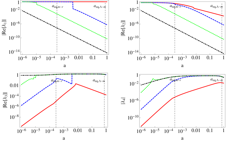
Figure 19: Eigenvalues for the reduced four dimensional system. The colour coding is the same as that in figure 2. The eigenvalue structure is different than that for the 5D system. In this case $\lambda_{4}$ is always real and hence no imaginary part. The imaginary part of $\lambda_{3}$ for the $k=100$ $h{\rm Mpc}^{-1}$ mode (black) is zero in the range of epochs shown.

References

- Alam et al. (2016) Alam S. et al., 2016, ArXiv e-prints, 1607, arXiv:1607.03155
- Arfken (2000) Arfken G., 2000, Mathematical Methods for Physicists. Academic Press Inc. San Diego, USA
- Bertschinger (1995) Bertschinger E., 1995, ArXiv Astrophysics e-prints, arXiv:astro
- Blas et al. (2011) Blas D., Lesgourgues J., Tram T., 2011, Journal of Cosmology and Astro-Particle Physics, 07, 034
- Burrage & Butcher (1979) Burrage K., Butcher J. C., 1979, SIAM Journal of Numerical Analysis, 16, 46
- Butcher (1987) Butcher J., 1987, The numerical analysis of ordinary differential equations. John Wiley & Sons Ltd.
- Collins & Akritas (1976) Collins G. E., Akritas A. G., 1976, Polynomial Real Root Isolation Using Descarte’s Rule of Signs, SYMSAC ’76. ACM, New York, NY, USA, pp. 272–275
- Cyr-Racine & Sigurdson (2011) Cyr-Racine F.-Y., Sigurdson K., 2011, Physical Review D, 83, 103521
- Dodelson (2003) Dodelson S., 2003, Modern Cosmology. Academic Press, Elsevier
- Doran (2005a) Doran M., 2005a, Journal of Cosmology and Astro-Particle Physics, 10, 011
- Doran (2005b) Doran M., 2005b, Journal of Cosmology and Astro-Particle Physics, 06, 011
- Harrier et al. (1996) Harrier E., Nørsett S., Wanner G., 1996, Solving Ordinary Differential Equations I, edition. Springer Series in Computational Mathematics
- Harrier & Wanner (1996) Harrier E., Wanner G., 1996, Solving Ordinary Differential Equations II, edition. Springer Series in Computational Mathematics
- Hook & McAree (1990) Hook D. G., McAree P. R., 1990, Graphics Gems, edited by Glassner, Andrew S. Academic Press Professional, Inc., San Diego, CA, USA, pp. 416–422
- Hu et al. (1995) Hu W., Scott D., Sugiyama N., White M., 1995, Physical Review D, 52, 5498
- Hu et al. (1998) Hu W., Seljak U., White M., Zaldarriaga M., 1998, Physical Review D, 57, 3290
- Hu & Sugiyama (1995) Hu W., Sugiyama N., 1995, The Astrophysical Journal, 444, 489
- Hu & Sugiyama (1996) Hu W., Sugiyama N., 1996, The Astrophysical Journal, 471, 542
- Hu & White (1997) Hu W., White M., 1997, Physical Review D, 56, 596
- Kodama & Sasaki (1984) Kodama H., Sasaki M., 1984, Progress of Theoretical Physics Supplement, 78, 1
- Lambert (1992) Lambert J. D., 1992, Numerical Methods for Ordinary Differential Systems. Wiley, New York, USA.
- Lesgourgues (2011) Lesgourgues J., 2011, ArXiv e-prints, 1104, arXiv:1104.2932
- Lewis et al. (2000) Lewis A., Challinor A., Lasenby A., 2000, The Astrophysical Journal, 538, 473
- Ma & Bertschinger (1995) Ma C.-P., Bertschinger E., 1995, The Astrophysical Journal, 455, 7
- Meszaros (1974) Meszaros P., 1974, Astronomy and Astrophysics, 37, 225
- Nicola et al. (2016a) Nicola A., Refregier A., Amara A., 2016a, Physical Review D, 94, 083517
- Nicola et al. (2016b) Nicola A., Refregier A., Amara A., 2016b, ArXiv e-prints, 1612, arXiv:1612.03121
- Petzold & Ascher (1998) Petzold L., Ascher U. M., 1998, The numerical analysis of ordinary differential equations. Society for Industrial and Applied Mathematics (SIAM)
- Planck Collaboration et al. (2016) Planck Collaboration et al., 2016, Astronomy and Astrophysics, 594, A13
- Press et al. (2002) Press W., Teukolsky S., Vetterling W., Flannery B., 2002, Numerical Recipes in C++. Cambridge University Press
- Seljak (1996) Seljak U., 1996, The Astrophysical Journal, 463, 1
- Seljak (1997) Seljak U., 1997, The Astrophysical Journal, 482, 6
- Seljak et al. (2003) Seljak U., Sugiyama N., White M., Zaldarriaga M., 2003, Physical Review D, 68, 083507
- Seljak & Zaldarriaga (1996) Seljak U., Zaldarriaga M., 1996, The Astrophysical Journal, 469, 437
- Shampine & Reichelt (1997) Shampine L. F., Reichelt M. W., 1997, SIAM J. Sci. Comput., 18, 1
- Slotine & Weiping (1991) Slotine J. E., Weiping L., 1991, Applied non-linear control. Prentice-Hall Inc., Englewood Cliffs, New Jersey 07632 USA
- Strogatz (1994) Strogatz S. H., 1994, Non-linear dynamics and chaos. Perseus Publishing, Cambridge, Massachusets
- Sugiyama (1989) Sugiyama N., 1989, Progress of Theoretical Physics, 81, 1021
- Sugiyama (1995) Sugiyama N., 1995, The Astrophysical Journal Supplement Series, 100, 281
- Sugiyama & Gouda (1992) Sugiyama N., Gouda N., 1992, Progress of Theoretical Physics, 88, 803
- Weinberg (2002) Weinberg S., 2002, The Astrophysical Journal, 581, 810
- White & Scott (1996) White M., Scott D., 1996, The Astrophysical Journal, 459, 415
- Wolfram Research (2008) Wolfram Research I., 2008, Mathematica Edition: Version 7.0.1. Wolfram Research, Inc. Place of publication: Champaign, Illinois
- Zaldarriaga & Seljak (1998) Zaldarriaga M., Seljak U., 1998, Physical Review D, 58, 023003
- Zaldarriaga & Seljak (2000) Zaldarriaga M., Seljak U., 2000, The Astrophysical Journal Supplement Series, 129, 431