Graphene Nano-Ribbons: Major differences in the fundamental gap as its length is increased either in the zig-zag or the armchair directions

Abstract

Controlling the forbidden gap of graphene nano-ribbons (GNR) is a major challenge that has to be attained if this attractive material has to be used in micro- and nano-electronics. Using an unambiguous notation {m,n}-GNR, where $m(n)$ is the number of six carbon rings in the arm-chair (zig-zag) directions, we investigate how varies the HOMO-LUMO gap when the size of the GNR is varied by increasing either $m$ or $n$, while keeping the other variable fixed. It is shown that no matter whether charge- or spin-density-waves solutions are considered, the gap varies smoothly when $n$ is kept fixed whereas it oscillates when the opposite is done, posing serious difficulties to the control of the gap. It is argued that the origin of this behavior is the fact that excess or defect charges or magnetic moments are mostly localised at zig-zag edges.

I Introduction

Major improvements in bottom-up tecnologies are allowing the fabrication of Graphene Nano-Ribbons (GNR) with well-defined shape and size WT16 ; TR16 ; WZ16 ; XL16 ; YL16 ; WC15 ; LG14 ; CO13 ; TS13 ; RC12 ; VC15 ; KA12 ; BP13 . This is opening the possibility of controlling the forbidden band gap KA12 ; SC06a ; SC06b and, thus, widen the range of technological applications of graphene CG09 ; DA11 ; LV07 . Measuring the nanoribbon conductance and/or using Scanning Tunneling Spectroscopy (STS) to determine the Local Density of States (LDOS) have allowed the researchers obtaining valuable information on the electronic structure around the HOMO-LUMO gap. Results have been already published for 7-AGNR (see below for notation) WT16 ; TS13 ; KA12 ; RC12 and 13-AGNR CO13 .

Although most data were taken on ribbons adsorbed on (111) surface of fcc metals, very specially on Au(111) KA12 ; RC12 ; CO13 ; TS13 ; LC14 , recently, several auhors have been able to lift off the surface a single graphene nanoribbon KA12 ; BP13 ; WT16 by controlled pulling of one of the ribbon’s ends using a STM. This technique is being applied to a variety of studies of considerable interest TR16 ; XL16 : i) keeping one of the GNR’s end attached to the tip the ribbon was characterized before and after lifting by imaging and spectroscopy KA12 , ii) a reliable transfer process of the lifted layer has allowed the investigation of the transistor performance of GNR BP13 , iii) more recently, transferring the GNR to a thin NaCl deposit onto a gold substrate has allowed, according to the authors of Ref. [WT16, ], a reliable characterization of the electronic structure of the ribbon. Several techniques have been developed to produce GNR free of defects XL16 , albeit in most cases GNR are fabricated by means of bottom-up techniques on metal (preferently gold) surfaces and with the help of STM WT16 ; TR16 ; XL16 ; CO13 . Recently etching of larger pieces of graphene has also been utilized LC14 . Alhough these techniques have, up to recently, only been applied to fabricate ribbons with arm-chair edges and rather narrow in the zig-zag direction, several works have been published in the current year that, modifying the procedures used to fabricate GNR with arm-chair edges, reports successful fabrication of ribbons with zig-zag edges WT16 ; TR16 ; LC14 . The strategy followed in those works consists of growing the ribbon not along the direction of the carbon–halogen bond, but at an angle of either 30 or 90 to it. The method, altnough not free of vacancies and kinks that distort the edges, has a reasonable reliability having allowed topological and spectroscopic studies LC14 .

In the present work we investigate how the forbidden gap (actually the HOMO-LUMO gap) varies as a function of the nano-ribbon length for several widths and either zig-zag or arm-chair edges. Albeit in the latter case the gap varies smoothly with the ribbon’s length, in the former it oscillates making far more difficult obtaining ribbons with a defined gap width.The reason for this harmful behavior is that either staggered magnetization or charges are mostly located in the zig-zag edges. Then, if increasing the ribbon length does not imply varying the number of zig-zag atoms one may expect a rather constant gap. The opposite should occur when length is increased along the zig-zag direction. Our numerical results confirm these conjectures. Although in our previous work we discarded spin polarised solutions arguing that, i) once the mono-determinantal approximation for the many-body wavefunction is abandoned it is likely that charge density wave (CDW) solutions become more favorable, and ii) no experimental evidence of spin-polarized edges has been found whatsoever WT16 , in this work spin density wave (SDW) solutions are also considered as they have been investigated by many different theory groups.

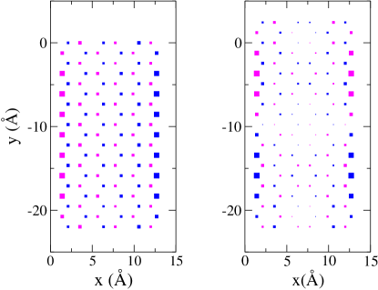
Figure 1: (Color online) Illustrates the notation used in this work to denote finite Graphene-Nano-Ribbons (GNR). Those shown in the Figure are {3,9}-GNR (left) and {3,10}-GNR (right), repectively. In addition, each axis has to be associated with a particular edge type; in our case we choose the $x$ axis to correspond to the armchair edge and the $y$ axis to the zig-zag edge. In the more standard notation of Ref. [SC06a, ] the cluster shown in the left (right) panel may either be 19-AGNR (21-AGNR) or 6-ZGNR (Z and A standing for zig-zag and armchair, respectively). The local $z$ component of the spin ($S_{z}$) of two SDW (spin density wave) solutions denoted AF1-SDW (left) and SF0-SDW (right), see text, that differ in energy less than 0.002% is also shown; Symbol size is proportional to actual spin and color denotes up or down $S_{z}$. CDW solutions with similar arrangements of excess and defect charges are also found (see text). Maximum staggered magnetization 0.313.

II Hamiltonian, procedures and notation

II.1 The Pariser,Pople, Parr (PPP) Hamiltonian

In this work we use the model Hamiltonian proposed by Pariser, Parr and Pople (PPP model) PP53 ; Po53 , solved within the Unrestricted Hartree-Fock (UHF) approximation (see below), that has been sucessfully applied to investigate the electronic structure of PAH CL15 .The PPP model includes both local on-site and long-range Coulomb interactions. Only a single $\pi$ orbital per atom is considered. The PPP Hamiltonian contains a non-interacting part $\hat{H}_{0}$ and a second term incorporating electron-electron interactions $\hat{H}_{I}$:

$${\hat{H}}={\hat{H}_{0}}+{\hat{H}_{I}}\;.$$ (1)

Eventually, a core, constant term may be added to account for the contribution of the rest of non-$\pi$ electrons to the total energyVC09 ; VS09 ; VS10 ; SG11 . The non-interacting term is written as:

$${\hat{H}_{0}}=\epsilon_{0}\sum_{i=1,N;\sigma}{\hat{c}}^{\dagger}_{i\sigma}{\hat{c}}_{i\sigma}+\sum_{<ij>;\sigma}t_{ij}{\hat{c}}^{\dagger}_{i\sigma}{\hat{c}}_{j\sigma}\;,$$ (2)

where the operator ${\hat{c}}^{\dagger}_{i\sigma}$ creates an electron at site $i$ with spin $\sigma$, $\epsilon_{0}$ is the energy of the orbital, $N$ is the number of orbitals and $t_{ij}$ is the hopping between nearest neighbor pairs $<\!\!ij\!\!>$ (kinetic energy).

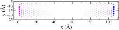
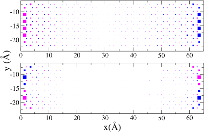
Figure 2: (Color online) Local distribution of the $z$-component of the spin $S_{z}$ in $\{15,6\}$ (two lower pictures) and $\{25,6\}$ (upper picture). Anti-symmetric solutions correspond to either A0-SDW (lower picture) or A1-SDW (upper and middle pictures). Maximum staggered magnetization 0.35 (upper and center) and 0.52 (lower).

In cases where the distance $d_{ij}$ between nearest neighbors pairs $<\!\!ij\!\!>$ significantly varies over the system, the hopping parameter may be scaled. For instance in some PAH or even in defective graphene the C-C distance may differ from its standard value $d_{0}=1.41$ Å. In such cases one may use a scaling adequate for $\pi$ orbitals Pa86 , namely

$$t_{ij}=\left(\frac{d_{0}}{d_{ij}}\right)^{3}t_{0}\;,$$ (3)

where $t_{0}$ is a fitting parameter. The assumption in using scaling laws is that the interatomic distance will always be close to $d_{0}$, as occurs in most cases.

The interacting part is given by:

$${\hat{H}_{I}}=U\sum_{i=1,N}{\hat{n}}_{i\uparrow}{\hat{n}}_{i\downarrow}+{\frac{1}{2}}\sum_{i,j=1,N;i\neq j}V_{ij}({\hat{n}}_{i}-1)({\hat{n}}_{j}-1)\;,$$ (4)

where $U$ is the on-site Coulomb repulsion, $V_{ij}$ is the inter-site Coulomb repulsion and the total electron density for site $i$ is

$${\hat{n}}_{i}={\hat{n}}_{i\uparrow}+{\hat{n}}_{i\downarrow}\;,$$ (5)

In incorporating the Coulomb interaction $V_{ij}$ one may choose the unscreened Coulomb interaction Ma00 , although it is a common practice the use of some interpolating formula. In the case of PAH that proposed by OhnoOh64 has a wide acceptance,

$$V_{ij}=U\left[1+\left(\frac{U}{e^{2}/d_{ij}}\right)^{2}\right]^{-1/2}\;.$$ (6)

Using this interpolation scheme implies that no additional parameter is introduced and, consequently, $U$ remains as the single parameter associated to interactions.

II.2 Cluster Notation

The notation used to identify graphene nano-ribbons (GNR) is illustrated in Figs. (1) and (2). Actually is identical to that proposed in Ref. [WC15, ]. Each GNR is characterised by two indexes $\{m,n\}$ denoting the number of benzene rings in the armchair direction $m$ (or $x$ direction) and the zig-zag $n$ (or $y$ direction). This avoids possible ambiguities derived from an earlier and widely used notation which explicitly referred to arm-chair GNR ($N_{z}$-AGNR) or zig-zag GNR ($N_{a}$-ZGNR) ribbons SC06a . It is useful connecting the present notation with the latter one proposed to name infinitely long ribbons (in infinitely long ribbons the ambiguities mentioned in the caption of Figs. (1) do not longer show up. In a ribbon infinitely long in the arm-chair (zig-zag) direction $N_{a}=2n+1$ ($N_{z}=2m$), where $N_{a}$ ($N_{z}$) the number of edge atoms in each case. The advantages of the notation used here are clearly illustrated in the just mentioned Figures.

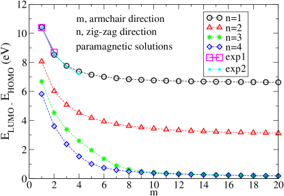
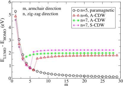
Figure 3: (Color online) Calculated $E_{LUMO}-E_{HOMO}$ for paramagnetic solutions in GNR of dimensions $\{1-20,1-4\}$ (upper) and $\{1-28,5\}$ (lower) and A-CDW solutions in GNR of dimensions $\{1-28,6-7\}$. In the case of $\{1-28,7\}$ resuts for both A-CDW and S-CDW solutions are shown. Experimental results for GNR of dimensions $\{1-4,1\}$ [SK84, ,SS94, ,MD83, ,NA06, ,RT02, ] are included in the upper plot (see also [YL16, ]).

II.3 Procedures

As noted above, in this work, the PPP Hamiltonian has been solved within the UHF approximation. All two operators terms (as given by Wick’s theorem) conserving charge and spin have been included: The non-diagonal term plays an important role whenever crystalline periodicity is absent. These includes interaction between distant defects, presence of impurities or surfaces, etc.SS10 ; CL15 . The correct description of small finite systems like GNRs also requires such a careful description.

The parameter values used hereafter have been derived from exact solutions of many spin states of neutral and charged small molecules SG11 ; VC09 ; VS09 ; VS10 . They are: $\epsilon_{0}$=-7.61 eV, $t_{0}$=-2.34 eV and $U$=8.29 eV. Clusters containing up to about 1000 $\pi$–orbitals have been investigated in this work. This has required the use of a simplified treatment of interactions such as Hartree-Fock (HF). Nonetheless, we shall show that even at such low level of approximation it is possible, in this case, to attain results that throw light on experimental data and/or more sophisticated theoretical calculations. All ribbons here investigated had the edge dangling $\sigma$ bonds passivated by hydrogen atoms.

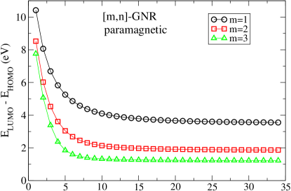
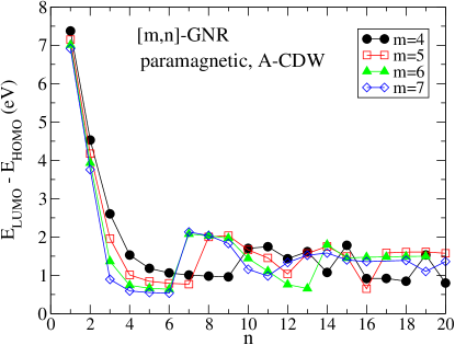
Figure 4: (Color online)Calculated $E_{LUMO}-E_{HOMO}$ for paramagnetic solutions in GNR of dimensions $\{1-3,1-34\}$ (upper) and A-CDW solutions (for $n\leq$ 6-9, depending on $m$, the solution is paramagnetic) in $\{4-7,1-20\}$ GNR (lower).

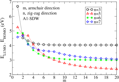
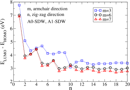
Figure 5: (Color online) Calculated $E_{LUMO}-E_{HOMO}$ for antiferromagnetic solutions in GNR of dimensions $\{1-20,(3,5-7)\}$ (upper) and $\{(3,6,7),1-20\}$ (lower). In the first case (upper panel) solutions are always of the A1-SDW type but for the smallest $m$ which show no magnetic polarization. In the second case, however, transitions between A0- and A1-SDW solutions occur as $n$ increases (these solutions differ less than 0.02% in energy). See also Fig. 1.

II.4 Mean field solutions notation

Three types of electronic configurations are obtained by solving UHF-PPP on GNR, namely, paramagnetic (P), Charge Density Waves (CDW) and Spin Density Waves (SDW). First note that the P configuration here obtained slightly differs from the strictly free electron solution ($U$ =0); this is due to the non-diagonal terms that the most general UHF approximation of the PPP model includes (see preceeding subsection). As regards charge and spin density waves solutions they can be classified as: S-CDW symmetric upon reflection through the $y$ axis passing by the center of the ribbon (no excess charge in both zig-zag edges). A-CDW anti-symmetric upon reflection through the $y$ axis passing by the center of the ribbon (excess or defect charge at the two edges, although neutral the two halves of the GNR). A1-SDW anti-symmetric upon reflection through the $y$ axis passing by the center of the ribbon, positive $z$ component of the spin $S_{z}$ in one edge and negative at the opposite. A0-SDW anti-symmetric upon reflection through the $y$ axis passing by the center of the ribbon, but total $z$ component of the spin $S_{z}=0$ on both edges. The SDW solutions are illustrated in Figs. (1) and (2) of this work and the CDW solutions in Fig. 9 of Ref. [VC15, ], This notation will be used hereafter.

III Results

Fig. 3 shows the results for $\{m,1-7\}$-GNR. For $m\leq 5$, the gap decreases monotonically and smoothly with the ribbon length (or, equivalently, $m$). Apparently, for $n$=1,2 (upper panel) the gap tends to a constant as $m$ increases, while it tends to zero for $n$=3-5. Beyond $n$=5 (lower panel), the CDW shows up VC15 for a length $m$ that decreases as $n$ increases. The emergence of the A-CDW implies an abrupt increase of the gap. Beyond this sharp increase the gap varies smoothly, almost remaining constant, with the ribbon length. As shown in the upper panel of the Figure, the calculated gap for $n$=1 is in excellent agreement with the available experimental data SK84 ; SS94 ; MD83 ; NA06 ; RT02 . Finally, in the lower panel of the Figure, the results for the S-CDW solution in the ribbon with $n$=7 are also depicted. It should be noted that albeit the gap in the symmetric solution is 0.24 eV higher than in the A-CDW solution, their energies differ in this case in less than 0.01%,

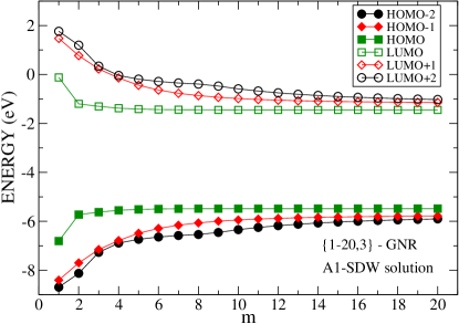
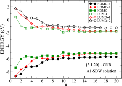
Figure 6: (Color online) Energies of the three upper HOMO and the three lower LUMO versus the nanoribbon length in the armchair direction ($m$). The results correspond to A1-SDW solutions of the PPP Hamiltonian on $\{1-20,6\}$ graphene nanoribbons (see Fig. 1 for notation).

It is pertinent comparing the present results with those reported by Yeh and Lee YL16 for the {20,1}-GNR, obtained with a variety of KS-DFT based methods. The results for the magnitude named by the authors $E_{g}(3)$, identical to that plotted in Fig. 3, are depicted in Fig. 6c of Ref. [YL16, ]. Only the results obtained from the $\omega$B97 and $\omega$B97X functionals do reasonably agree with the available experimental data, although not as much as the results presented here as they are slightly higher.

Fig. 4 shows the results for $\{1-7,n\}$-GNR. In this case the ribbon is paramagnetic for $m$=1-3 and all values of $n$ shown in the Figure. As in the previous case, the gaps decrease smoothly and monotonically with $n$. However, it cannot be concluded whether they will or they will not vanish for infinitely long ribbons. On the other hand, for $n>3$ and a value of $m$ that decreases as $n$ increases, the charge density wave shows up. Beyond that point the gap oscillates in an unpredictable manner. These oscillations are surely due to the increase of the number of edge states with $n$ SC06a .

We turn now to discuss the characteristics of the spin polarised solutions. Fig (5) shows te gap in {1-20,3-7}-GNR and {3-7,1-20}-GNR. In the first case, whereby the ribbon grows in the armchair direction at constant width, the gap varies smoothly with $m$ decreasing monotonically beyond $m>2$, coinciding with the size at which the SDW replaces the paramagnetic solution. In addition it varies in a manner consistent with the results reported in Ref. [SC06a, ], namely, the gap of the three families that can be differentiated goes as gap ($2n=3p$) $>$ gap($2n=3p-1$)$>$ gap($2n=3p-1$), where $p$ is an integer. Moreover, within each family the gap decreases with the ribbon wdith, compare results for $n$=3 with those for $n$=6. This qualitative agreement (remind that ribbons in Ref. [SC06a, ] are infinite in one direction) is found for the LDA results reported in that work and not for those obtained with a one-electron tight-binding method which, among other features, predict a zero gap for the $3p+1$ family, no matter the ribbon width. Recent studies of $\{m,3\}$ WT16 with $m$ up to 48 provided the following results: i) experimental data (GW calculations) gave a gap between states localised at zig-zag edges of 1.8 (2.8) eV, a result almost independent of ribbon length, and, ii) a delocalised (or bulk) states gap that did vary with the ribbon length being around 2.8 eV for $m=48$. Our calculations gave larger gaps around 4 (4.8) for localised (bulk) states that did not vary (decrease) with the ribbon length.

It should be mentioned that all results shown in the Figure correspond to A1-SDW solutions (left panel in Fig. 1 and upper and midle panels in Fig. 2). This solution shows, as discussed in Ref. [SC06b, ], half-metallicity. However, as already mentioned here, there is another SDW solution, referred to as A0-SDW, which has an energy very close to that of A1-SDW (only 0.002% higher) that, having a null total $z$-component of the spin on the zig-zag edge atoms (see right panel in Fig. 1 and lower panel in Fig. 2), cannot show half-metallicity.

Results for the gap in {3-7,1-20}-GNR are shown in the lower panel of Fig (5). As in the previous case, the gap decreases with the ribbon length $n$, however a dramatic change is noted, namely, the smooth decrease observed beyond $m>2$ in{1-20,3-7}-GNR, is replaced by oscillations as already observed in the case of CDW solutions. Confirming this behavior experimentally will discard this type of ribbon for technological applications note .

The three HOMO having the highest energy and the three LUMO having the lower one are plotted in Fig. 6 versus the ribbon length, for {1-20,3}-GNR and {3,1-20}-GNR. Again it is noted that while in the first case energy levels, and in particular the band gap, vary (actually decrease) smoothly with the ribbon length $m$, in the second case they oscillate in an irregular manner (in comparing results of Fig. 6 with those of Fig. (5) note that the energy range in the former is twice that in the latter). Finally it is worth mentioning that while for $n>15$ the two lower LUMO and two upper HOMO are almost degenerate, no degeneration is observed in ribbons elongated in the armchair direction {1-20,3}-GNR. This is in agreement with results reported in Refs. [NF96, ,YP07, ].

Fig. 7 shows the energy difference between A-CDW and A1-SDW solutions (see text) in GNR of dimensions $\{1-20,6\}$. For $m\leq 7$ the paramagnetic solution has no CDW, whereas the SDW solution shows up for $m>2$. This explains the irregular behavior of the energy difference at small $m$. Beyond $m=7$, the straight lines fitted to the energies are consistent with the slow decrease of the energy difference as the ribbon length increases (small discrepancies should be ascribed to the fact that while energies vary over thousands of eV, they differ only in approximately 2 eV, i.e, less than 0.07%). This small energy difference, whose order of magnitude does not vary dramatically with ribbon size, may justify our conjecture concerning the possibility that many body interactions may favor the CDW solutions.

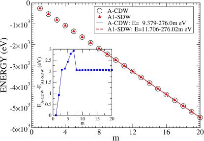
Figure 7: (Color online) Energy difference between A-CDW and A1-SDW solutions (see text) in GNR of dimensions $\{1-20,6\}$. For $m\leq 7$ the paramagnetic solution has no CDW.

IV Concluding Remarks

Graphene nanoribbons are one of the best founded hopes for a major jump in the microelectronics (nanoelectronics?) industry. Initial attempts of fabrication of nanoribbons found many dificulties that hindered obtaining GNR with well-defined shape and size. Very recently, the development of a variety of bottom-up techniques have led to the reliable production of not only ribbonns with arm-chair edges but also the far more difficult with zig-zag edges. Despite of the good performance of that technique, full control of ribbon shappe and length is not always easy. Avoiding the presence at the ribbon edges of vacancies and kinks is still a major problem. This may be the main cause of discrepancies that still exist amongst different laboratories. In addition, the large variety of theoretical tools used to tackle the problem not always agree The main result reported here concerns the different behavior of the energy gap vs ribbon length found for ribbons enlarged either in the armchair or the zig-zag directions. While in the former the gap varies smoothly with the length, it oscillates appreciably in the latter. Unfortunately we do not have any experimental support for this conclusion as most of the experimental studies concern ribbons with length varying in the arm-chair direction. A major unresolved question is whether there is any spin polarisation at the zig-zag edges. All mono-determinantal calculations, the present one included, indicate that it actually should be. However, as discussed here, charge and spin density waves solutions differ in few eV, while the total ribbon energy soon reaches ten thousand eV, making possible that many-body effects invert that order. As regards experimental verification, there is not yet a trustable strategy to explore the low energy spin physics at graphene nano-ribbons.

- (1) S. Wang, L. Talirz, C. A. Pignedoli, X. Feng, K. Mu llen, R. Fasel and P. Ruffieux, Nature Commun., DOI: 10.1038/ncomms11507 (2016).
- (2) L. Talirz, P. Ruffieux and R. Fasel, Adv. Mater. 28, 6222 (2016).
- (3) W.-X. Wang, M. Zhou, X. Li, S.-Y. Li, X. Wu, W. Duan, and L. He, Phys. Rev. B 93, 241403(R) (2016).
- (4) W. Xu and T.-W. Lee. Mater. Horiz. 3 186 (2016).
- (5) C.-N. Yeh, P.-Y. Lee, and J.-D. Chai, arXiv:1601.04205v2 [physics.chem-ph] 28 Apr 2016.
- (6) C.-S. Wu and J.-D. Chai, J. Chem. Theory Comput. 11, 2003 (2015).
- (7) S. Li, C. K. Gan, Y.-W. Son d, Y. P. Feng S. Y. Quek, Carbon 76, 285 ( 2014).
- (8) Y.C. Chen, D.G. de Oteyza, Z. Pedramrazi, C. Chen, F.R. Fischer and M.F. Crommie, ACS Nano 7, 6123 (2013).
- (9) L. Talirz, H. Sode, J.M. Cai, P. Ruffieux, S. Blankenburg, R. Jafaar, R. Berger, X. Feng, K. Mullen, D. Passerone, R. Fasel and C.A. Pignedoli, J. Am. Chem. Soc. 135, 2060 (2013).
- (10) P. Ruffieux, J.M. Cai, N.C. Plumb, L. Patthey, D. Prezzi, A. Ferretti, E. Molinari, X.L. Feng, K. Mullen, C.A. Pignedoli and R. Fasel, ACS Nano 6, 6930 (2012).
- (11) J.A. Vergés, G. Chiappe, and E. Louis, Eur. Phys. J. B 88, 200 (2015).
- (12) M. Koch, F. Ample, C. Joachim, L. Grill, Nat. Nanotech. 7, 713 (2012).
- (13) P.B. Bennett, Z. Pedramrazi, A. Madani, Y.C. Chen, D.G. de Oteyza, C. Chen, F.R. Fischer, M.F. Crommie, and J. Bokor, Appl. Phys. Lett. 103, 253114 (2013).
- (14) Y.-W. Son, M. L. Cohen, S. G. Louie, Phys. Rev. Lett. 97, 216803 (2006).
- (15) Y.-W. Son, M. L. Cohen and S. G. Louie, Nature 444, 347 (2006).
- (16) A.H. Castro Neto, F. Guinea, N.M.R. Peres, K.S. Novoselov, A.K. Geim, Rev. Mod. Phys. 81, 109 (2009) and references therein.
- (17) S. Das Sarma, S. Adam, E.H. Hwan and E. Rossi, Rev Mod. Phys. 83, 407 (2011) and references therein.
- (18) E. Louis, J.A. Vergés, F. Guinea, G. Chiappe, Phys. Rev. B 75, 085440 (2007).
- (19) Y.Y. Li, M.X. Cen, M. Weinert, L. Li, Nature Commun. 5, 4311 (2014).
- (20) R. Pariser and R.G. Parr, J. Chem. Phys. 21 466 (1953).
- (21) J.A. Pople, Trans. Faraday Soc. 49 1365 (1953).
- (22) D. Baereswyl, J. Carmelo, D.K. Campbell, F. Guinea and E. Louis, eds., The Hubbard Model: Its Physics and Mathematical Physics, NATO ASI Series Vol. 343, (Plenum Press, New York, 1995).
- (23) K. Gundra, A. Shukla, Phys. Rev. 83, 075413 (2011).
- (24) K. Gundra, A. Shukla, Phys. Rev. 84, 075442 (2011).
- (25) P. Sony, A. Shukla, Computer Phys. Commun. 181, 821 (2010).
- (26) P. Potasz, A. D. Güçlü, A. Wójs, and P. Hawrylak, Phys. Rev. B 85, 075431 (2012).
- (27) M. Hohenadler, S. Wessel, M. Daghofer, and F. F. Assaad, Phys. Rev. B 85, 195115 (2012).
- (28) E. San-Fabián, A. Guijarro, J.A. Vergés, G. Chiappe and E. Louis, Eur. Phys. J. B 81, 253 (2011).
- (29) J.A. Vergés, G. Chiappe, E. Louis, L. Pastor-Abia and E. San-Fabián, Phys. Rev. B 79, 094403 (2009).
- (30) J.A. Vergés, E. San-Fabián, L. Pastor-Abia, G. Chiappe and E. Louis, Phys. Stat. Solidi C 6, 2139 (2009).
- (31) J.A. Vergés, E. San-Fabián, G. Chiappe and E. Louis, Phys. Rev. B 81, 085120 (2010).
- (32) G. Chiappe, E. Louis, E. San-Fabián and J.A. Vergés, J. Phys.: Condens. Matter 27, 463001 (2015).
- (33) D.A. Papaconstantopoulos, Handbook of the Band Structure of Elemental Solids (Plenum Press, New York, 1986).
- (34) G.D. Mahan, Many-Particle Physics (Kluwer Academic/Plenum Publishers, New York, 2000).
- (35) K. Ohno, Theor. Chim. Acta 2 219 (1964).
- (36) F. Moscardó, E. San-Fabián, Chem. Phys. Lett. 480, 26 (2009).
- (37) K. Seki, U. O. Karlsson, R. Engelhardt, E. E. Koch, W. Schmidt, Chem. Phys. 91, 459 (1984).
- (38) S. W. Staley, J. T. Strnad, J. Phys. Chem. 98, 116 (1994).
- (39) A. Modelli, G. Distefano, D. Jones, Chem. Phys. 82, 489 (1983).
- (40) T. Nakamura, N. Ando, Y. Matsumoto, S. Furuse, M. Mitsui, A. Nakajima, Chem. Lett. 35, 888 (2006).
- (41) J. C. Rienstra-Kiracofe, G. S. Tschumper, H. F. Schaefer III, S. Nandi, G. B. Ellison, Chem. Rev. 102, 231 (2002).
- (42) It should be noted that the way we increase the size of the ribbon is that followed by the experimental techniques nowadays available WT16 . This may imply changing the family of the ribbon as defined in Ref. [YP07, ].
- (43) K. Nakada, M. Fujita, G. Dresselhaus, M.S. Dresselhaus, Phys. Rev. B 54, 17954 (1996).
- (44) L. Yang, C.-H. Park, Y.-W. Son, M.L. Cohen, S.G. Louie, Phys. Rev. Lett. 99, 186801 (2007).