Four lectures on probabilistic methods for data science

Abstract.

Methods of high-dimensional probability play a central role in applications for statistics, signal processing, theoretical computer science and related fields. These lectures present a sample of particularly useful tools of high-dimensional probability, focusing on the classical and matrix Bernstein’s inequality and the uniform matrix deviation inequality. We illustrate these tools with applications for dimension reduction, network analysis, covariance estimation, matrix completion and sparse signal recovery. The lectures are geared towards beginning graduate students who have taken a rigorous course in probability but may not have any experience in data science applications.

1. Lecture 1: Concentration of sums of independent random variables

These lectures present a sample of modern methods of high dimensional probability and illustrate these methods with applications in data science. This sample is not comprehensive by any means, but it could serve as a point of entry into a branch of modern probability that is motivated by a variety of data-related problems.

To get the most out of these lectures, you should have taken a graduate course in probability, have a good command of linear algebra (including the singular value decomposition) and be familiar with very basic concepts of functional analysis (familiarity with $L^{p}$ norms should be enough).

All of the material of these lectures is covered more systematically, at a slower pace, and with a wider range of applications, in my forthcoming textbook [60]. You may also be interested in two similar tutorials: [58] is focused on random matrices, and a more advanced text [59] discusses high-dimensional inference problems.

It should be possible to use these lectures for a self-study or group study. You will find here many places where you are invited to do some work (marked in the text e.g. by “check this!”), and you are encouraged to do it to get a better grasp of the material. Each lecture ends with a section called “Notes” where you will find bibliographic references of the results just discussed, as well asvarious improvements and extensions.

We are now ready to start.

Probabilistic reasoning has a major impact on modern data science. There are roughly two ways in which this happens.

• Radnomized algorithms, which perform some operations at random, have long been developed in computer science and remain very popular. Randomized algorithms are among the most effective methods – and sometimes the only known ones – for many data problems.

• Random models of data form the usual premise of statistical analysis. Even when the data at hand is deterministic, it is often helpful to think of it as a random sample drawn from some unknown distribution (“population”).

In these lectures, we will encounter both randomized algorithms and random models of data.

1.1. Sub-gaussian distributions

Before we start discussing probabilistic methods, we will introduce an important class of probability distributions that forms a natural “habitat” for random variables in many theoretical and applied problems. These are sub-gaussian distributions. As the name suggests, we will be looking at an extension of the most fundamental distribution in probability theory – the gaussian, or normal, distribution $N(\mu,\sigma)$.

It is a good exercise to check that the standard normal random variable $X\sim N(0,1)$ satisfies the following basic properties:

Tails:

$\mathbb{P}\left\{|X|\geq t\rule{0.0pt}{8.53581pt}\right\}\leq 2\exp(-t^{2}/2)$ for all $t\geq 0$.

Moments:

$\|X\|_{p}:=(\operatorname{\mathbb{E}}|X|^{p})^{1/p}=O(\sqrt{p})$ as $p\to\infty$.

MGF of square:

$\operatorname{\mathbb{E}}\exp(cX^{2})\leq 2$ for some $c>0$.

MGF:

$\operatorname{\mathbb{E}}\exp(\lambda X)=\exp(\lambda^{2})$ for all $\lambda\in\mathbb{R}$.

All these properties tell the same story from four different perspectives. It is not very difficult to show (although we will not do it here) that for any random variable $X$, not necessarily Gaussian, these four properties are essentially equivalent.

Proposition 1 (Sub-gaussian properties).

For a random variable $X$, the following properties are equivalent.

Tails:

$\mathbb{P}\left\{|X|\geq t\rule{0.0pt}{8.53581pt}\right\}\leq 2\exp(-t^{2}/K_{1}^{2})$ for all $t\geq 0$.

Moments:

$\|X\|_{p}\leq K_{2}\sqrt{p}$ for all $p\geq 1$.

MGF of square:

$\operatorname{\mathbb{E}}\exp(X^{2}/K_{3}^{2})\leq 2$.

Moreover, if $\operatorname{\mathbb{E}}X=0$ then these properties are also equivalent to the following one:

MGF:

$\operatorname{\mathbb{E}}\exp(\lambda X)\leq\exp(\lambda^{2}K_{4}^{2})$ for all $\lambda\in\mathbb{R}$.

Random variables that satisfy one of the first three properties (and thus all of them) are called sub-gaussian. The best $K_{3}$ is called the sub-gaussian norm of $X$, and is usually denoted $\|X\|_{\psi_{2}}$, that is

$$\|X\|_{\psi_{2}}:=\inf\left\{t>0:\;\operatorname{\mathbb{E}}\exp(X^{2}/t^{2})\leq 2\right\}.$$

One can check that $\|\cdot\|_{\psi_{2}}$ indeed defines a norm; it is an example of the general concept of the Orlicz norm. Proposition 1 states that the numbers $K_{i}$ in all four properties are equivalent to $\|X\|_{\psi_{2}}$ up to absolute constant factors.

Example 2.

As we already noted, the standard normal random variable $X\sim N(0,1)$ is sub-gaussian. Similarly, arbitrary normal random variables $X\sim N(\mu,\sigma)$ are sub-gaussian. Another example is a Bernoulli random variable $X$ that takes values $0$ and $1$ with probabilities $1/2$ each. More generally, any bounded random variable $X$ is sub-gaussian. On the contrary, Poisson, exponential, Pareto and Cauchy distributions are not sub-gaussian. (Verify all these claims; this is not difficult.)

1.2. Hoeffding’s inequality

You may remember from a basic course in probability that the normal distribution $N(\mu,\sigma)$ has a remarkable property: the sum of independent normal random variables is also normal. Here is a version of this property for sub-gaussian distributions.

Proposition 3 (Sums of sub-gaussians).

Let $X_{1},\ldots,X_{N}$ be independent, mean zero, sub-gaussian random variables. Then $\sum_{i=1}^{N}X_{i}$ is a sub-gaussian, and

$$\Big{\|}\sum_{i=1}^{N}X_{i}\Big{\|}_{\psi_{2}}^{2}\leq C\sum_{i=1}^{N}\|X_{i}\|_{\psi_{2}}^{2}$$

where $C$ is an absolute constant.

Proof.

Let us bound the moment generating function of the sum for any $\lambda\in\mathbb{R}$:

$$\operatorname{\mathbb{E}}\exp\big{(}\lambda\sum_{i=1}^{N}X_{i}\big{)} =\prod_{i=1}^{N}\operatorname{\mathbb{E}}\exp(\lambda X_{i})\quad\text{(using independence)}$$

$$\leq\prod_{i=1}^{N}\exp(C\lambda^{2}\|X_{i}\|_{\psi_{2}}^{2})\quad\text{(by last property in Proposition\leavevmode\nobreak\ \ref{prop: sub-gaussian})}$$

$$=\exp(\lambda^{2}K^{2})\quad\text{where }K^{2}:=C\sum_{i=1}^{N}\|X_{i}\|_{\psi_{2}}^{2}.$$

Using again the last property in Proposition 1, we conclude that the sum $S=\sum_{i=1}^{N}X_{i}$ is sub-gaussian, and $\|S\|_{\psi_{2}}\leq C_{1}K$ where $C_{1}$ is an absolute constant. The proof is complete. ∎

Let us rewrite Proposition 3 in a form that is often more useful in applications, namely as a concentration inequality. To do this, we simply use the first property in Proposition 1 for the sum $\sum_{i=1}^{N}X_{i}$. We immediately get the following.

Theorem 4 (General Hoeffding’s inequality).

Let $X_{1},\ldots,X_{N}$ be independent, mean zero, sub-gaussian random variables. Then, for every $t\geq 0$ we have

$$\mathbb{P}\Big{\{}\Big{|}\sum_{i=1}^{N}X_{i}\Big{|}\geq t\Big{\}}\leq 2\exp\Big{(}-\frac{ct^{2}}{\sum_{i=1}^{N}\|X_{i}\|_{\psi_{2}}^{2}}\Big{)}.$$

Hoeffding’s inequality controls how far and with what probability a sum of independent random variables can deviate from its mean, which is zero.

1.3. Sub-exponential distributions

Sub-gaussian distributions form a sufficiently wide class of distributions. Many results in probability and data science are proved nowadays for sub-gaussian random variables. Still, as we noted, there are some natural random variables that are not sub-gaussian. For example, the square $X^{2}$ of a normal random variable $X\sim N(0,1)$ is not sub-gaussian. (Check!) To cover examples like this, we will introduce the similar but weaker notion of sub-exponential distributions.

Proposition 5 (Sub-exponential properties).

For a random variable $X$, the following properties are equivalent, in the same sense as in Proposition 1.

Tails:

$\mathbb{P}\left\{|X|\geq t\rule{0.0pt}{8.53581pt}\right\}\leq 2\exp(-t/K_{1})$ for all $t\geq 0$.

Moments:

$\|X\|_{p}\leq K_{2}p$ for all $p\geq 1$.

MGF of the square:

$\operatorname{\mathbb{E}}\exp(|X|/K_{3})\leq 2$.

Moreover, if $\operatorname{\mathbb{E}}X=0$ then these properties imply the following one:

MGF:

$\operatorname{\mathbb{E}}\exp(\lambda X)\leq\exp(\lambda^{2}K_{4}^{2})$ for $|\lambda|\leq 1/K_{4}$.

Just like we did for sub-gaussian distributions, we call the best $K_{3}$ the sub-exponential norm of $X$ and denote it by $\|X\|_{\psi_{1}}$, that is

$$\|X\|_{\psi_{1}}:=\inf\left\{t>0:\;\operatorname{\mathbb{E}}\exp(|X|/t)\leq 2\right\}.$$

All sub-exponential random variables are squares of sub-gaussian random variables. Indeed, inspecting the definitions you will quickly see that

(6) $$\|X^{2}\|_{\psi_{1}}=\|X\|_{\psi_{2}}^{2}.$$

(Check!)

1.4. Bernstein’s inequality

A version of Hoeffding’s inequality for sub-exponential random variables is called Bernstein’s inequality. You may naturally expect to see a sub-exponential tail bound in this result. So it may come as a surprise that Bernstein’s inequality actually has a mixture of two tails – sub-gaussian and sub-exponential. Let us state and prove the inequality first, and then we will comment on the mixture of the two tails.

Theorem 7 (Bernstein’s inequality).

Let $X_{1},\ldots,X_{N}$ be independent, mean zero, sub-exponential random variables. Then, for every $t\geq 0$ we have

$$\mathbb{P}\Big{\{}\Big{|}\sum_{i=1}^{N}X_{i}\Big{|}\geq t\Big{\}}\leq 2\exp\Big{[}-c\min\Big{(}\frac{t^{2}}{\sum_{i=1}^{N}\|X_{i}\|_{\psi_{1}}^{2}},\;\frac{t}{\max_{i}\|X_{i}\|_{\psi_{1}}}\Big{)}\Big{]}.$$

Proof.

For simplicity, we will assume that $K=1$ and only prove the one-sided bound (without absolute value); the general case is not much harder. Our approach will be based on bounding the moment generating function of the sum $S:=\sum_{i=1}^{N}X_{i}$. To see how MGF can be helpful here, choose $\lambda\geq 0$ and use Markov’s inequality to get

(8) $$\mathbb{P}\left\{S\geq t\rule{0.0pt}{8.53581pt}\right\}=\mathbb{P}\left\{\exp(\lambda S)\geq\exp(\lambda t)\rule{0.0pt}{8.53581pt}\right\}\leq e^{-\lambda t}\operatorname{\mathbb{E}}\exp(\lambda S).$$

Recall that $S=\sum_{i=1}^{N}X_{i}$ and use independence to express the right side of (8) as

$$e^{-\lambda t}\prod_{i=1}^{N}\operatorname{\mathbb{E}}\exp(\lambda X_{i}).$$

(Check!) It remains to bound the MGF of each term $X_{i}$, and this is a much simpler task. If we choose $\lambda$ small enough so that

(9) $$0<\lambda\leq\frac{c}{\max_{i}\|X_{i}\|_{\psi_{1}}},$$

then we can use the last property in Proposition 5 to get

$$\operatorname{\mathbb{E}}\exp(\lambda X_{i})\leq\exp\big{(}C\lambda^{2}\|X_{i}\|_{\psi_{1}}^{2}\big{)}.$$

Substitute into (8) and conclude that

$$\mathbb{P}\{S\geq t\}\leq\exp\left(-\lambda t+C\lambda^{2}\sigma^{2}\right)$$

where $\sigma^{2}=\sum_{i=1}^{N}\|X_{i}\|_{\psi_{1}}^{2}$. The left side does not depend on $\lambda$ while the right side does. So we can choose $\lambda$ that minimizes the right side subject to the constraint (9). When this is done carefully, we obtain the tail bound stated in Bernstein’s inequality. (Do this!) ∎

Now, why does Bernstein’s inequality have a mixture of two tails? The sub-exponential tail should of course be there. Indeed, even if the entire sum consisted of a single term $X_{i}$, the best bound we could hope for would be of the form $\exp(-ct/\|X_{i}\|_{\psi_{1}})$. The sub-gaussian term could be explained by the central limit theorem, which states that the sum should becomes approximately normal as the number of terms $N$ increases to infinity.

Remark 10 (Bernstein’s inequality for bounded random variables).

Suppose the random variables $X_{i}$ are uniformly bounded, which is a stronger assumption than being sub-gaussian. Then there is a useful version of Bernstein’s inequality, which unlike Theorem 7 is sensitive to the variances of $X_{i}$’s. It states that if $K>0$ is such that $|X_{i}|\leq K$ almost surely for all $i$, then, for every $t\geq 0$, we have

(11) $$\mathbb{P}\Big{\{}\Big{|}\sum_{i=1}^{N}X_{i}\Big{|}\geq t\Big{\}}\leq 2\exp\Big{(}-\frac{t^{2}/2}{\sigma^{2}+CKt}\Big{)}.$$

Here $\sigma^{2}=\sum_{i=1}^{N}\operatorname{\mathbb{E}}X_{i}^{2}$ is the variance of the sum. This version of Bernstein’s inequality can be proved in essentially the same way as Theorem 7. We will not do it here, but a stronger Theorem 20, which is valid for matrix-valued random variables $X_{i}$, will be proved in Lecture 2.

To compare this with Theorem 7, note that $\sigma^{2}+CKt\leq 2\max(\sigma^{2},CKt)$. So we can state the probability bound (11) as

$$2\exp\Big{[}-c\min\Big{(}\frac{t^{2}}{\sigma^{2}},\;\frac{t}{K}\Big{)}\Big{]}.$$

Just like before, here we also have a mixture of two tails, sub-gaussian and sub-exponential. The sub-gaussian tail is a bit sharper than in Theorem 7, since it depends on the variances rather than sub-gaussian norms of $X_{i}$. The sub-exponential tail, on the other hand, is weaker, since it depends on the sup-norms rather than the sub-exponential norms of $X_{i}$.

1.5. Sub-gaussian random vectors

The concept of sub-gaussian distributions can be extended to higher dimensions. Consider a random vector $X$ taking values in $\mathbb{R}^{n}$. We call $X$ a sub-gaussian random vector if all one-dimensional marginals of $X$, i.e., the random variables $\left\langle X,x\right\rangle$ for $x\in\mathbb{R}^{n}$, are sub-gaussian. The sub-gaussian norm of $X$ is defined as

$$\|X\|_{\psi_{2}}:=\sup_{x\in S^{n-1}}\|\left\langle X,x\right\rangle\|_{\psi_{2}}$$

where $S^{n-1}$ denotes the unit Euclidean sphere in $\mathbb{R}^{n}$.

Example 12.

Examples of sub-gaussian random distributions in $\mathbb{R}^{n}$ include the standard normal distribution $N(0,I_{n})$ (why?), the uniform distribution on the centered Euclidean sphere of radius $\sqrt{n}$, the uniform distribution on the cube $\{-1,1\}^{n}$, and many others. The last example can be generalized: a random vector $X=(X_{1},\ldots,X_{n})$ with independent and sub-gaussian coordinates is sub-gaussian, with $\|X\|_{\psi_{2}}\leq C\max_{i}\|X_{i}\|_{\psi_{2}}$.

1.6. Johnson-Lindenstrauss Lemma

Concentration inequalities like Hoeffding’s and Bernstein’s are successfully used in the analysis of algorithms. Let us give one example for the problem of dimension reduction. Suppose we have some data that is represented as a set of $N$ points in $\mathbb{R}^{n}$. (Think, for example, of $n$ gene expressions of $N$ patients.)

We would like to compress the data by representing it in a lower dimensional space $\mathbb{R}^{m}$ instead of $\mathbb{R}^{n}$ with $m\ll n$. By how much can we reduce the dimension without loosing the important features of the data?

The basic result in this direction is the Johnson-Lindenstrauss Lemma. It states that a remarkably simple dimension reduction method works – a random linear map from $\mathbb{R}^{n}$ to $\mathbb{R}^{m}$ with

$$m\sim\log N,$$

see Figure 1. The logarithmic function grows very slowly, so we can usually reduce the dimension dramatically.

What exactly is a random linear map? Several models are possible to use. Here we will model such a map using a Gaussian random matrix – an $m\times n$ matrix $A$ with independent $N(0,1)$ entries. More generally, we can consider an $m\times n$ matrix $A$ whose rows are independent, mean zero, isotropic and sub-gaussian random vectors in $\mathbb{R}^{n}$. For example, the entries of $A$ can be independent Rademacher entries – those taking values $\pm 1$ with equal probabilities.

Theorem 13 (Johnson-Lindenstrauss Lemma).

Let $\mathcal{X}$ be a set of $N$ points in $\mathbb{R}^{n}$ and $\varepsilon\in(0,1)$. Consider an $m\times n$ matrix $A$ whose rows are independent, mean zero, isotropic and sub-gaussian random vectors in $\mathbb{R}^{n}$. Rescale $A$ by defining the “Gaussian random projection”

$$P:=\frac{1}{\sqrt{m}}A.$$

Assume that

$$m\geq C\varepsilon^{-2}\log N,$$

where $C$ is an appropriately large constant that depends only on the sub-gaussian norms of the vectors $X_{i}$. Then, with high probability (say, $0.99$), the map $P$ preserves the distances between all points in $\mathcal{X}$ with error $\varepsilon$, that is

(14) $$(1-\varepsilon)\|x-y\|_{2}\leq\|Px-Py\|_{2}\leq(1+\varepsilon)\|x-y\|_{2}\quad\text{for all }x,y\in\mathcal{X}.$$

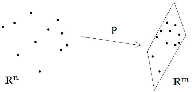
Figure 1. Johnson-Lindenstrauss Lemma states that a random projection of $N$ data points from dimension $n$ to dimension $m\sim\log N$ approximately preserves the distances between the points.

Proof.

Take a closer look at the desired conclusion (14). By linearity, $Px-Py=P(x-y)$. So, dividing the inequality by $\|x-y\|_{2}$, we can rewrite (14) in the following way:

(15) $$1-\varepsilon\leq\|Pz\|_{2}\leq 1+\varepsilon\quad\text{for all }z\in T$$

where

$$T:=\left\{\frac{x-y}{\|x-y\|_{2}}:\;x,y\in\mathcal{X}\text{ distinct points}\right\}.$$

It will be convenient to square the inequality (15). Using that $1+\varepsilon\leq(1+\varepsilon)^{2}$ and $1-\varepsilon\geq(1-\varepsilon)^{2}$, we see that it is enough to show that

(16) $$1-\varepsilon\leq\|Pz\|_{2}^{2}\leq 1+\varepsilon\quad\text{for all }z\in T.$$

By construction, the coordinates of the vector $Pz=\frac{1}{\sqrt{m}}Az$ are $\frac{1}{\sqrt{m}}\left\langle X_{i},z\right\rangle$. Thus we can restate (16) as

(17) $$\Big{|}\frac{1}{m}\sum_{i=1}^{m}\left\langle X_{i},z\right\rangle^{2}-1\Big{|}\leq\varepsilon\quad\text{for all }z\in T.$$

Results like (17) are often proved by combining concentration and a union bound. In order to use concentration, we first fix $z\in T$. By assumption, the random variables $\left\langle X_{i},z\right\rangle^{2}-1$ are independent; they have zero mean (use isotropy to check this!), and they are sub-exponential (use (6) to check this). Then Bernstein’s inequality (Theorem 7) gives

$$\mathbb{P}\left\{\Big{|}\frac{1}{m}\sum_{i=1}^{m}\left\langle X_{i},z\right\rangle^{2}-1\Big{|}>\varepsilon\rule{0.0pt}{8.53581pt}\right\}\leq 2\exp(-c\varepsilon^{2}m).$$

(Check!)

Finally, we can unfix $z$ by taking a union bound over all possible $z\in T$:

$$\mathbb{P}\left\{\max_{z\in T}\Big{|}\frac{1}{m}\sum_{i=1}^{m}\left\langle X_{i},z\right\rangle^{2}-1\Big{|}>\varepsilon\rule{0.0pt}{8.53581pt}\right\} \leq\sum_{z\in T}\mathbb{P}\left\{\Big{|}\frac{1}{m}\sum_{i=1}^{m}\left\langle X_{i},z\right\rangle^{2}-1\Big{|}>\varepsilon\rule{0.0pt}{8.53581pt}\right\}$$

(18) $$\leq|T|\cdot 2\exp(-c\varepsilon^{2}m).$$

By definition of $T$, we have $|T|\leq N^{2}$. So, if we choose $m\geq C\varepsilon^{-2}\log N$ with appropriately large constant $C$, we can make (18) bounded by $0.01$. The proof is complete. ∎

1.7. Notes

The material presented in Sections 1.1–1.5 is basic and can be found e.g. in [58] and [60] with all the proofs. Bernstein’s and Hoeffding’s inequalities that we covered here are two basic examples of concentration inequalities. There are many other useful concentration inequalities for sums of independent random variables (e.g. Chernoff’s and Bennett’s) and for more general objects. The textbook [60] is an elementary introduction into concentration; the books [10, 39, 38] offer more comprehensive and more advanced accounts of this area.

The original version of Johnson-Lindenstrauss Lemma was proved in [31]. The version we gave here, Theorem 13, was stated with probability of success $0.99$, but an inspection of the proof gives probability $1-2\exp(-c\varepsilon^{2}m)$ which is much better for large $m$. A great variety of ramifications and applications of Johnson-Lindenstrauss lemma are known, see e.g. [42, 2, 4, 7, 10, 34].

2. Lecture 2: Concentration of sums of independent random matrices

In the previous lecture we proved Bernstein’s inequality, which quantifies how a sum of independent random variables concentrates about its mean. We will now study an extension of Bernstein’s inequality to higher dimensions, which holds for sums of independent random matrices.

2.1. Matrix calculus

The key idea of developing a matrix Bernstein’s inequality will be to use matrix calculus, which allows us to operate with matrices as with scalars – adding and multiplying them of course, but also comparing matrices and applying functions to matrices. Let us explain this.

We can compare matrices to each other using the notion of being positive semidefinite. Let us focus here on $n\times n$ symmetric matrices. If $A-B$ is a positive semidefinite matrix, which we denote $A-B\succeq 0$, then we say that $A\succeq B$ (and, of course, $B\preceq A$). This defines a partial order on the set of $n\times n$ symmetric matrices. The term “partial” indicates that, unlike the real numbers, there exist $n\times n$ symmetric matrices $A$ and $B$ that can not be compared. (Give an example where neither $A\preceq B$ nor $B\succeq A$!)

Next, let us guess how to measure the magnitude of a matrix $A$. The magnitude of a scalar $a\in\mathbb{R}$ is measured by the absolute value $|a|$; it is the smallest non-negative number $t$ such that

$$-t\leq a\leq t.$$

Extending this reasoning to matrices, we can measure the magnitude of an $n\times n$ symmetric matrix $A$ by the smallest non-negative number $t$ such that

$$-tI_{n}\preceq A\preceq tI_{n}.$$

The smallest $t$ is called the operator norm of $A$ and is denoted $\|A\|$. Diagonalizing $A$, we can see that

(19) $$\|A\|=\max\{|\lambda|:\;\text{$\lambda$ is an eigenvalue of $A$}\}.$$

With a little more work (do it!), we can see that $\|A\|$ is the norm of $A$ acting as a linear operator on the Euclidean space $(\mathbb{R}^{n},\|\cdot\|_{2})$; this is why $\|A\|$ is called the operator norm. Thus $\|A\|$ is the smallest non-negative number $M$ such that

$$\|Ax\|_{2}\leq M\|x\|_{2}\quad\text{for all }x\in\mathbb{R}^{n}.$$

Finally, we will need to be able to take functions of matrices. Let $f:\mathbb{R}\to\mathbb{R}$ be a function and $X$ be an $n\times n$ symmetric matrix. We can define $f(X)$ in two equivalent ways. The spectral theorem allows us to represent $X$ as

$$X=\sum_{i=1}^{n}\lambda_{i}u_{i}u_{i}^{\mathsf{T}}$$

where $\lambda_{i}$ are the eigenvalues of $X$ and $u_{i}$ are the corresponding eigenvectors. Then we can simply define

$$f(X):=\sum_{i=1}^{n}f(\lambda_{i})u_{i}u_{i}^{\mathsf{T}}.$$

Note that $f(X)$ has the same eigenvectors as $X$, but the eigenvalues change under the action of $f$. An equivalent way to define $f(X)$ is using power series. Suppose the function $f$ has a convergent power series expansion about some point $x_{0}\in\mathbb{R}$, i.e.

$$f(x)=\sum_{k=1}^{\infty}a_{k}(x-x_{0})^{k}.$$

Then one can check that the following matrix series converges and defines $f(X)$:

$$f(X)=\sum_{k=1}^{\infty}a_{k}(X-X_{0})^{k}.$$

(Check!)

2.2. Matrix Bernstein’s inequality

We are now ready to state and prove a remarkable generalization of Bernstein’s inequality for random matrices.

Theorem 20 (Matrix Bernstein’s inequality).

Let $X_{1},\ldots,X_{N}$ be independent, mean zero, $n\times n$ symmetric random matrices, such that $\|X_{i}\|\leq K$ almost surely for all $i$. Then, for every $t\geq 0$ we have

$$\mathbb{P}\Big{\{}\Big{\|}\sum_{i=1}^{N}X_{i}\Big{\|}\geq t\Big{\}}\leq 2n\cdot\exp\Big{(}-\frac{t^{2}/2}{\sigma^{2}+Kt/3}\Big{)}.$$

Here $\sigma^{2}=\left\|\sum_{i=1}^{N}\operatorname{\mathbb{E}}X_{i}^{2}\right\|$ is the norm of the “matrix variance” of the sum.

The scalar case, where $n=1$, is the classical Bernstein’s inequality we stated in (11). A remarkable feature of matrix Bernstein’s inequality, which makes it especially powerful, is that it does not require any independence of the entries (or the rows or columns) of $X_{i}$; all is needed is that the random matrices $X_{i}$ be independent from each other.

In the rest of this section we will prove matrix Bernstein’s inequality, and give a few applications in this and next lecture.

Our proof will be based on bounding the moment generating function (MGF) $\operatorname{\mathbb{E}}\exp(\lambda S)$ of the sum $S=\sum_{i=1}^{N}X_{i}$. Note that to exponentiate the matrix $\lambda S$ in order to define the matrix MGF, we rely on the matrix calculus that we introduced in Section 2.1.

If the terms $X_{i}$ were scalars, independence would yield the classical fact that the MGF of a product is the product of MGF’s, i.e.

(21) $$\operatorname{\mathbb{E}}\exp(\lambda S)=\operatorname{\mathbb{E}}\prod_{i=1}^{N}\exp(\lambda X_{i})=\prod_{i=1}^{N}\operatorname{\mathbb{E}}\exp(\lambda X_{i}).$$

But for matrices, this reasoning breaks down badly, for in general

$$e^{X+Y}\neq e^{X}e^{Y}$$

even for $2\times 2$ symmetric matrices $X$ and $Y$. (Give a counterexample!)

Fortunately, there are some trace inequalities that can often serve as proxies for the missing equality $e^{X+Y}=e^{X}e^{Y}$. One of such proxies is the Golden-Thompson inequality, which states that

(22) $$\operatorname{tr}(e^{X+Y})\leq\operatorname{tr}(e^{X}e^{Y})$$

for any $n\times n$ symmetric matrices $X$ and $Y$. Another result, which we will actually use in the proof of matrix Bernstein’s inequality, is Lieb’s inequality.

Theorem 23 (Lieb’s inequality).

Let $H$ be an $n\times n$ symmetric matrix. Then the function

$$f(X)=\operatorname{tr}\exp(H+\log X)$$

is concave on the space on $n\times n$ symmetric matrices.

Note that in the scalar case, where $n=1$, the function $f$ in Lieb’s inequality is linear and the result is trivial.

To use Lieb’s inequality in a probabilistic context, we will combine it with the classical Jensen’s inequality. It states that for any concave function $f$ and a random matrix $X$, one has

(24) $$\operatorname{\mathbb{E}}f(X)\leq f(\operatorname{\mathbb{E}}X).$$

Using this for the function $f$ in Lieb’s inequality, we get

$$\operatorname{\mathbb{E}}\operatorname{tr}\exp(H+\log X)\leq\operatorname{tr}\exp(H+\log\operatorname{\mathbb{E}}X).$$

And changing variables to $X=e^{Z}$, we get the following:

Lemma 25 (Lieb’s inequality for random matrices).

Let $H$ be a fixed $n\times n$ symmetric matrix and $Z$ be an $n\times n$ symmetric random matrix. Then

$$\operatorname{\mathbb{E}}\operatorname{tr}\exp(H+Z)\leq\operatorname{tr}\exp(H+\log\operatorname{\mathbb{E}}e^{Z}).$$

Lieb’s inequality is a perfect tool for bounding the MGF of a sum of independent random variables $S=\sum_{i=1}^{N}X_{i}$. To do this, let us condition on the random variables $X_{1},\ldots,X_{N-1}$. Apply Lemma 25 for the fixed matrix $H:=\sum_{i=1}^{N-1}\lambda X_{i}$ and the random matrix $Z:=\lambda X_{N}$, and afterwards take the expectation with respect to $X_{1},\ldots,X_{N-1}$. By the law of total expectation, we get

$$\operatorname{\mathbb{E}}\operatorname{tr}\exp(\lambda S)\leq\operatorname{\mathbb{E}}\operatorname{tr}\exp\Big{[}\sum_{i=1}^{N-1}\lambda X_{i}+\log\operatorname{\mathbb{E}}e^{\lambda X_{N}}\Big{]}.$$

Next, apply Lemma 25 in a similar manner for $H:=\sum_{i=1}^{N-2}\lambda X_{i}+\log\operatorname{\mathbb{E}}e^{\lambda X_{N}}$ and $Z:=\lambda X_{N-1}$, and so on. After $N$ times, we obtain:

Lemma 26 (MGF of a sum of independent random matrices).

Let $X_{1},\ldots,X_{N}$ be independent $n\times n$ symmetric random matrices. Then the sum $S=\sum_{i=1}^{N}X_{i}$ satisfies

$$\operatorname{\mathbb{E}}\operatorname{tr}\exp(\lambda S)\leq\operatorname{tr}\exp\Big{[}\sum_{i=1}^{N}\log\operatorname{\mathbb{E}}e^{\lambda X_{i}}\Big{]}.$$

Think of this inequality is a matrix version of the scalar identity (21). The main difference is that it bounds the trace of the MGF rather the MGF itself.

You may recall from a course in probability theory that the quantity $\log\operatorname{\mathbb{E}}e^{\lambda X_{i}}$ that appears in this bound is called the cumulant generating function of $X_{i}$.

Lemma 26 reduces the complexity of our task significantly, for it is much easier to bound the cumulant generating function of each single random variable $X_{i}$ than to say something about their sum. Here is a simple bound.

Lemma 27 (Moment generating function).

Let $X$ be an $n\times n$ symmetric random matrix. Assume that $\operatorname{\mathbb{E}}X=0$ and $\|X\|\leq K$ almost surely. Then, for all $0<\lambda<3/K$ we have

$$\operatorname{\mathbb{E}}\exp(\lambda X)\preceq\exp\left(g(\lambda)\operatorname{\mathbb{E}}X^{2}\right)\quad\text{where}\quad g(\lambda)=\frac{\lambda^{2}/2}{1-\lambda K/3}.$$

Proof.

First, check that the following scalar inequality holds for $0<\lambda<3/K$ and $|x|\leq K$:

$$e^{\lambda x}\leq 1+\lambda x+g(\lambda)x^{2}.$$

Then extend it to matrices using matrix calculus: if $0<\lambda<3/K$ and $\|X\|\leq K$ then

$$e^{\lambda X}\preceq I+\lambda X+g(\lambda)X^{2}.$$

(Do these two steps carefully!) Finally, take the expectation and recall that $\operatorname{\mathbb{E}}X=0$ to obtain

$$\operatorname{\mathbb{E}}e^{\lambda X}\preceq I+g(\lambda)\operatorname{\mathbb{E}}X^{2}\preceq\exp\left(g(\lambda)\operatorname{\mathbb{E}}X^{2}\right).$$

In the last inequality, we use the matrix version of the scalar inequality $1+z\leq e^{z}$ that holds for all $z\in\mathbb{R}$. The lemma is proved. ∎

Proof of Matrix Bernstein’s inequality.

We would like to bound the operator norm of the random matrix $S=\sum_{i=1}^{N}X_{i}$, which, as we know from (19), is the largest eigenvalue of $S$ by magnitude. For simplicity of exposition, let us drop the absolute value from (19) and just bound the maximal eigenvalue of $S$, which we denote $\lambda_{\max}(S)$. (Once this is done, we can repeat the argument for $-S$ to reinstate the absolute value. Do this!) So, we are to bound

$$\mathbb{P}\left\{\lambda_{\max}(S)\geq t\rule{0.0pt}{8.53581pt}\right\} =\mathbb{P}\left\{e^{\lambda\cdot\lambda_{\max}(S)}\geq e^{\lambda t}\rule{0.0pt}{8.53581pt}\right\}\quad\text{(multiply by $\lambda>0$ and exponentiate)}$$

$$\leq e^{-\lambda t}\,\operatorname{\mathbb{E}}e^{\lambda\cdot\lambda_{\max}(S)}\quad\text{(by Markov's inequality)}$$

$$=e^{-\lambda t}\,\operatorname{\mathbb{E}}\lambda_{\max}(e^{\lambda S})\quad\text{(check!)}$$

$$\leq e^{-\lambda t}\,\operatorname{\mathbb{E}}\operatorname{tr}e^{\lambda S}\quad\text{(max of eigenvalues is bounded by the sum)}$$

$$\leq e^{-\lambda t}\operatorname{tr}\exp\Big{[}\sum_{i=1}^{N}\log\operatorname{\mathbb{E}}e^{\lambda X_{i}}\Big{]}\quad\text{(use Lemma\leavevmode\nobreak\ \ref{lem: MGF sum matrix})}$$

$$\leq\operatorname{tr}\exp\left[-\lambda t+g(\lambda)Z\right]\quad\text{(by Lemma\leavevmode\nobreak\ \ref{lem: matrix MGF})}$$

where

$$Z:=\sum_{i=1}^{N}\operatorname{\mathbb{E}}X_{i}^{2}.$$

It remains to optimize this bound in $\lambda$. The minimum is attained for $\lambda=t/(\sigma^{2}+Kt/3)$. (Check!) With this value of $\lambda$, we conclude

$$\mathbb{P}\left\{\lambda_{\max}(S)\geq t\rule{0.0pt}{8.53581pt}\right\}\leq n\cdot\exp\Big{(}-\frac{t^{2}/2}{\sigma^{2}+Kt/3}\Big{)}.$$

This completes the proof of Theorem 20. ∎

Bernstein’s inequality gives a powerful tail bound for $\|\sum_{i=1}^{N}X_{i}\|$. This easily implies a useful bound on the expectation:

Corollary 28 (Expected norm of sum of random matrices).

Let $X_{1},\ldots,X_{N}$ be independent, mean zero, $n\times n$ symmetric random matrices, such that $\|X_{i}\|\leq K$ almost surely for all $i$. Then

$$\operatorname{\mathbb{E}}\Big{\|}\sum_{i=1}^{N}X_{i}\Big{\|}\lesssim\sigma\sqrt{\log n}+K\log n$$

where $\sigma=\big{\|}\sum_{i=1}^{N}\operatorname{\mathbb{E}}X_{i}^{2}\big{\|}^{1/2}$.

Proof.

The link from tail bounds to expectation is provided by the basic identity

(29) $$\operatorname{\mathbb{E}}Z=\int_{0}^{\infty}\mathbb{P}\left\{Z>t\rule{0.0pt}{8.53581pt}\right\}\,dt$$

which is valid for any non-negative random variable $Z$. (Check it!) Integrating the tail bound given by matrix Bernstein’s inequality, you will arrive at the expectation bound we claimed. (Check!) ∎

Notice that the bound in this corollary has mild, logarithmic, dependence on the ambient dimension $n$. As we will see shortly, this can be an important feature in some applications.

2.3. Community recovery in networks

Matrix Bernstein’s inequality has many applications. The one we are going to discuss first is for the analysis of networks. A network can be mathematically represented by a graph, a set of $n$ vertices with edges connecting some of them. For simplicity, we will consider undirected graphs where the edges do not have arrows. Real world networks often tend to have clusters, or communities – subsets of vertices that are connected by unusually many edges. (Think, for example, about a friendship network where communities form around some common interests.) An important problem in data science is to recover communities from a given network.

We are going to explain one of the simplest methods for community recovery, which is called spectral clustering. But before we introduce it, we will first of all place a probabilistic model on the networks we consider. In other words, it will be convenient for us to view networks as random graphs whose edges are formed at random. Although not all real-world networks are truly random, this simplistic model can motivate us to develop algorithms that may empirically succeed also for real-world networks.

The basic probabilistic model of random graphs is the Erdös-Rényi model.

Definition 30 (Erdös-Rényi model).

Consider a set of $n$ vertices and connect every pair of vertices independently and with fixed probability $p$. The resulting random graph is said to follow the Erdös-Rényi model $G(n,p)$.

The Erdös-Rényi random model is very simple. But it is not a good choice if we want to model a network with communities, for every pair of vertices has the same chance to be connected. So let us introduce a natural generalization of the Erdös-Rényi random model that does allow for community structure:

Definition 31 (Stochastic block model).

Partition a set of $n$ vertices into two subsets (“communities”) with $n/2$ vertices each, and connect every pair of vertices independently with probability $p$ if they belong to the same community and $q<p$ if not. The resulting random graph is said to follow the stochastic block model $G(n,p,q)$.

Figure 2 illustrates a simulation of a stochastic block model.

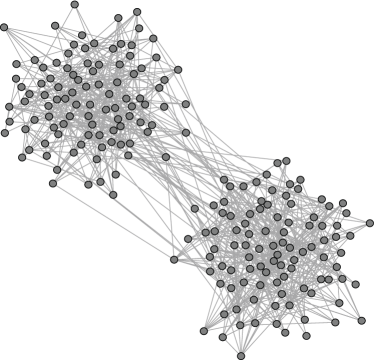
Figure 2. A network generated according to the stochastic block model $G(n,p,q)$ with $n=200$ nodes and connection probabilities $p=1/20$ and $q=1/200$.

Suppose we are shown one instance of a random graph generated according to a stochastic block model $G(n,p,q)$. How can we find which vertices belong to which community?

The spectral clustering algorithm we are going to explain will do precisely this. It will be based on the spectrum of the adjacency matrix $A$ of the graph, which is the $n\times n$ symmetric matrix whose entries $A_{ij}$ equal $1$ if the vertices $i$ and $j$ are connected by an edge, and $0$ otherwise.

The adjacency matrix $A$ is a random matrix. Let us compute its expectation first. This is easy, since the entires of $A$ are Bernoulli random variables. If $i$ and $j$ belong to the same community then $\operatorname{\mathbb{E}}A_{ij}=p$ and otherwise $\operatorname{\mathbb{E}}A_{ij}=q$. Thus $A$ has block structure: for example, if $n=4$ then $A$ looks like this:

$$\operatorname{\mathbb{E}}A=\left[\begin{array}[]{cc|cc}p&p&q&q\\ p&p&q&q\\ \hline\cr q&q&p&p\\ q&q&p&p\end{array}\right]$$

(For illustration purposes, we grouped the vertices from each community together.)

You will easily check that $A$ has rank $2$, and the non-zero eigenvalues and the corresponding eigenvectors are

(32) $$\lambda_{1}(\operatorname{\mathbb{E}}A)=\Big{(}\frac{p+q}{2}\Big{)}n,\quad v_{1}(\operatorname{\mathbb{E}}A)=\left[\begin{array}[]{c}1\\ 1\\ \hline\cr 1\\ 1\end{array}\right];\quad\lambda_{2}(\operatorname{\mathbb{E}}A)=\Big{(}\frac{p-q}{2}\Big{)}n,\quad v_{2}(\operatorname{\mathbb{E}}A)=\left[\begin{array}[]{r}1\\ 1\\ \hline\cr-1\\ -1\end{array}\right].$$

(Check!)

The eigenvalues and eigenvectors of $\operatorname{\mathbb{E}}A$ tell us a lot about the community structure of the underlying graph. Indeed, the first (larger) eigenvalue,

$$d:=\Big{(}\frac{p+q}{2}\Big{)}n,$$

is the expected degree of any vertex of the graph. The second eigenvalue tells us whether there is any community structure at all (which happens when $p\neq q$ and thus $\lambda_{2}(\operatorname{\mathbb{E}}A)\neq 0$). The first eigenvector $v_{1}$ is not informative of the structure of the network at all. It is the second eigenvector $v_{2}$ that tells us exactly how to separate the vertices into the two communities: the signs of the coefficients of $v_{2}$ can be used for this purpose.

Thus if we know $\operatorname{\mathbb{E}}A$, we can recover the community structure of the network from the signs of the second eigenvector. The problem is that we do not know $\operatorname{\mathbb{E}}A$. Instead, we know the adjacency matrix $A$. If, by some chance, $A$ is not far from $\operatorname{\mathbb{E}}A$, we may hope to use the $A$ to approximately recover the community structure. So is it true that $A\approx\operatorname{\mathbb{E}}A$? The answer is yes, and we can prove it using matrix Bernstein’s inequality.

Theorem 33 (Concentration of the stochastic block model).

Let $A$ be the adjacency matrix of a $G(n,p,q)$ random graph. Then

$$\operatorname{\mathbb{E}}\|A-\operatorname{\mathbb{E}}A\|\lesssim\sqrt{d\log n}+\log n.$$

Here $d=(p+q)n/2$ is the expected degree.

Proof.

Let us sketch the argument. To use matrix Bernstein’s inequality, let us break $A$ into a sum of independent random matrices

$$A=\sum_{i,j:\;i\leq j}X_{ij},$$

where each matrix $X_{ij}$ contains a pair of symmetric entries of $A$, or one diagonal entry. Matrix Bernstein’s inequality obviously applies for the sum

$$A-\operatorname{\mathbb{E}}A=\sum_{i\leq j}(X_{ij}-\operatorname{\mathbb{E}}X_{ij}).$$

Corollary 28 gives

(34) $$\operatorname{\mathbb{E}}\|A-\operatorname{\mathbb{E}}A\|\lesssim\sigma\sqrt{\log n}+K\log n$$

where $\sigma^{2}=\big{\|}\sum_{i\leq j}\operatorname{\mathbb{E}}(X_{ij}-\operatorname{\mathbb{E}}X_{ij})^{2}\big{\|}$ and $K=\max_{ij}\|X_{ij}-\operatorname{\mathbb{E}}X_{ij}\|$. It is a good exercise to check that

$$\sigma^{2}\lesssim d\quad\text{and}\quad K\leq 2.$$

(Do it!) Substituting into (34), we complete the proof. ∎

How useful is Theorem 33 for community recovery? Suppose that the network is not too sparse, namely

$$d\gg\log n.$$

Then

$$\|A-\operatorname{\mathbb{E}}A\|\lesssim\sqrt{d\log n}\quad\text{while}\quad\|\operatorname{\mathbb{E}}A\|=\lambda_{1}(\operatorname{\mathbb{E}}A)=d,$$

which implies that

$$\|A-\operatorname{\mathbb{E}}A\|\ll\|\operatorname{\mathbb{E}}A\|.$$

In other words, $A$ nicely approximates $\operatorname{\mathbb{E}}A$: the relative error or approximation is small in the operator norm.

At this point one can apply classical results from the perturbation theory for matrices, which state that since $A$ and $\operatorname{\mathbb{E}}A$ are close, their eigenvalues and eigenvectors must also be close. The relevant perturbation results are Weyl’s inequality for eigenvalues and Davis-Kahan’s inequality for eigenvectors, which we will not reproduce here. Heuristically, what they give us is

$$v_{2}(A)\approx v_{2}(\operatorname{\mathbb{E}}A)=\left[\begin{array}[]{r}1\\ 1\\ \hline\cr-1\\ -1\end{array}\right].$$

Then we should expect that most of the coefficients of $v_{2}(A)$ are positive on one community and negative on the other. So we can use $v_{2}(A)$ to approximately recover the communities. This method is called spectral clustering:

Spectral Clustering Algorithm. Compute $v_{2}(A)$, the eigenvector corresponding to the second largest eigenvalue of the adjacency matrix $A$ of the network. Use the signs of the coefficients of $v_{2}(A)$ to predict the community membership of the vertices.

We saw that spectral clustering should perform well for the stochastic block model $G(n,p,q)$ if it is not too sparse, namely if the expected degrees satisfy $d=(p+q)n/2\gg\log n$.

A more careful analysis along these lines, which you should be able to do yourself with some work, leads to the following more rigorous result.

Theorem 35 (Guarantees of spectral clustering).

Consider a random graph generated according to the stochastic block model $G(n,p,q)$ with $p>q$, and set $a=pn$, $b=qn$. Suppose that

(36) $$(a-b)^{2}\gg\log(n)(a+b).$$

Then, with high probability, the spectral clustering algorithm recovers the communities up to $o(n)$ misclassified vertices.

Note that condition (36) implies that the expected degrees are not too small, namely $d=(a+b)/2\gg\log(n)$ (check!). It also ensures that $a$ and $b$ are sufficiently different: recall that if $a=b$ the network is Erdös-Rényi graph without any community structure.

2.4. Notes

The idea to extend concentration inequalities like Bernstein’s to matrices goes back to R. Ahlswede and A. Winter [3]. They used Golden-Thompson inequality (22) and proved a slightly weaker form of matrix Bernstein’s inequality than we gave in Section 2.2. R. Oliveira [48, 49] found a way to improve this argument and gave a result similar to Theorem 20. The version of matrix Bernstein’s inequality we gave here (Theorem 20) and a proof based on Lieb’s inequality is due to J. Tropp [52].

The survey [53] contains a comprehensive introduction of matrix calculus, a proof of Lieb’s inequality (Theorem 23), a detailed proof of matrix Bernstein’s inequality (Theorem 20) and a variety of applications. A proof of Golden-Thompson inequality (22) can be found in [8, Theorem 9.3.7].

In Section 2.3 we scratched the surface of an interdisciplinary area of network analysis. For a systematic introduction into networks, refer to the book [47]. Stochastic block models (Definition 31) were introduced in [33]. The community recovery problem in stochastic block models, sometimes also called community detection problem, has been in the spotlight in the last few years. A vast and still growing body of literature exists on algorithms and theoretical results for community recovery, see the book [47], the survey [22], papers such as [61, 46, 32, 9, 37, 29, 30] and the references therein.

A concentration result similar to Theorem 33 can be found in [48]; the argument there is also based on matrix concentration. This theorem is not quite optimal. For dense networks, where the expected degree $d$ satisfies $d\gtrsim\log n$, the concentration inequality in Theorem 33 can be improved to

(37) $$\operatorname{\mathbb{E}}\|A-\operatorname{\mathbb{E}}A\|\lesssim\sqrt{d}.$$

This improved bound goes back to the original paper [21] which studies the simpler Erdös-Rényi model but the results extend to stochastic block models [17]; it can also be deduced from [6, 32, 37].

If the network is relatively dense, i.e. $d\gtrsim\log n$, one can improve the guarantee (36) of spectral clustering in Theorem 35 to

$$(a-b)^{2}\gg(a+b).$$

All one has to do is use the improved concentration inequality (37) instead of Theorem 33. Furthermore, in this case there exist algorithms that can recover the communities exactly, i.e. without any misclassified vertices, and with high probability, see e.g. [43, 32, 1, 17].

For sparser networks, where $d\ll\log n$ and possibly even $d=O(1)$, relativelyfew algorithms were known until recently, but now there exist many approaches that provably recover communities in sparse stochastic block models, see e.g. [46, 9, 17, 37, 29, 30, 61].

3. Lecture 3: Covariance estimation and matrix completion

In the last lecture, we proved matrix Bernstein’s inequality and gave an application for network analysis. We will spend this lecture discussing a couple of other interesting applications of matrix Bernstein’s inequality. In Section 3.1 we will work on covariance estimation, a basic problem in high-dimensional statistics. In Section 3.2, we will derive a useful bound on norms of random matrices, which unlike Bernstein’s inequality does not require any boundedness assumptions on the distribution. We will apply this bound in Section 3.3 for a problem of matrix completion, where we are shown a small sample of the entries of a matrix and asked to guess the missing entries.

3.1. Covariance estimation

Covariance estimation is a problem of fundamental importance in high-dimensional statistics. Suppose we have a sample of data points $X_{1},\ldots,X_{N}$ in $\mathbb{R}^{n}$. It is often reasonable to assume that these points are independently sampled from the same probability distribution (or “population”) which is unknown. We would like to learn something useful about this distribution.

Denote by $X$ a random vector that has this (unknown) distribution. The most basic parameter of the distribution is the mean $\operatorname{\mathbb{E}}X$. One can estimate $\operatorname{\mathbb{E}}X$ from the sample by computing the sample mean $\frac{1}{N}\sum_{i=1}^{N}X_{i}$. The law of large numbers guarantees that the estimate becomes tight as the sample size $N$ grows to infinity, i.e.

$$\frac{1}{N}\sum_{i=1}^{N}X_{i}\to\operatorname{\mathbb{E}}X\quad\text{as }N\to\infty.$$

The next most basic parameter of the distribution is the covariance matrix

$$\Sigma:=\operatorname{\mathbb{E}}(X-\operatorname{\mathbb{E}}X)(X-\operatorname{\mathbb{E}}X)^{\mathsf{T}}.$$

This is a higher-dimensional version of the usual notion of variance of a random variable $Z$, which is

$$\operatorname{Var}(Z)=\operatorname{\mathbb{E}}(Z-\operatorname{\mathbb{E}}Z)^{2}.$$

The eigenvectors of the covariance matrix of $\Sigma$ are called the principal components. Principal components that correspond to large eigenvalues of $\Sigma$ are the directions in which the distribution of $X$ is most extended, see Figure 3. These are often the most interesting directions in the data. Practitioners often visualize the high-dimensional data by projecting it onto the span of a few (maybe two or three) of such principal components; the projection may reveal some hidden structure of the data. This method is called Principal Component Analysis (PCA).

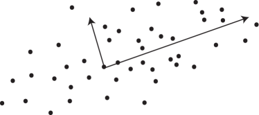
Figure 3. Data points $X_{1},\ldots,X_{N}$ sampled from a distribution in $\mathbb{R}^{n}$ and the principal components of the covariance matrix.

One can estimate the covariance matrix $\Sigma$ from the sample by computing the sample covariance

$$\Sigma_{N}:=\frac{1}{N}\sum_{i=1}^{N}(X_{i}-\operatorname{\mathbb{E}}X_{i})(X_{i}-\operatorname{\mathbb{E}}X_{i})^{\mathsf{T}}.$$

Again, the law of large numbers guarantees that the estimate becomes tight as the sample size $N$ grows to infinity, i.e.

$$\Sigma_{N}\to\Sigma\quad\text{as }N\to\infty.$$

But how large should the sample size $N$ be for covariance estimation? Generally, one can not have $N<n$ for dimension reasons. (Why?) We are going to show that

$$N\sim n\log n$$

is enough. In other words, covariance estimation is possible with just logarithmic oversampling.

For simplicity, we shall state the covariance estimation bound for mean zero distributions. (If the mean is not zero, we can estimate it from the sample and subtract. Check that the mean can be accurately estimated from a sample of size $N=O(n)$.)

Theorem 38 (Covariance estimation).

Let $X$ be a random vector in $\mathbb{R}^{n}$ with covariance matrix $\Sigma$. Suppose that

(39) $$\|X\|_{2}^{2}\lesssim\operatorname{\mathbb{E}}\|X\|_{2}^{2}=\operatorname{tr}\Sigma\quad\text{almost surely}.$$

Then, for every $N\geq 1$, we have

$$\operatorname{\mathbb{E}}\|\Sigma_{N}-\Sigma\|\lesssim\|\Sigma\|\;\Big{(}\sqrt{\frac{n\log n}{N}}+\frac{n\log n}{N}\Big{)}.$$

Before we pass to the proof, let us note that Theorem 38 yields the covariance estimation result we promised. Let $\varepsilon\in(0,1)$. If we take a sample of size

$$N\sim\varepsilon^{-2}n\log n,$$

then we are guaranteed covariance estimation with a good relative error:

$$\operatorname{\mathbb{E}}\|\Sigma_{N}-\Sigma\|\leq\varepsilon\|\Sigma\|.$$

Proof.

Apply matrix Bernstein’s inequality (Corollary 28) for the sum of independent random matrices $X_{i}X_{i}^{\mathsf{T}}-\Sigma$ and get

(40) $$\operatorname{\mathbb{E}}\|\Sigma_{N}-\Sigma\|=\frac{1}{N}\operatorname{\mathbb{E}}\Big{\|}\sum_{i=1}^{N}(X_{i}X_{i}^{\mathsf{T}}-\Sigma)\Big{\|}\lesssim\frac{1}{N}\big{(}\sigma\sqrt{\log n}+K\log n\big{)}$$

where

$$\sigma^{2}=\Big{\|}\sum_{i=1}^{N}\operatorname{\mathbb{E}}(X_{i}X_{i}^{\mathsf{T}}-\Sigma)^{2}\Big{\|}=N\big{\|}\operatorname{\mathbb{E}}(XX^{\mathsf{T}}-\Sigma)^{2}\big{\|}$$

and $K$ is chosen so that

$$\|XX^{\mathsf{T}}-\Sigma\|\leq K\quad\text{almost surely}.$$

It remains to bound $\sigma$ and $K$. Let us start with $\sigma$. We have

$$\operatorname{\mathbb{E}}(XX^{\mathsf{T}}-\Sigma)^{2} =\operatorname{\mathbb{E}}\|X\|_{2}^{2}XX^{\mathsf{T}}-\Sigma^{2}\quad\text{(check by expanding the square)}$$

$$\precsim\operatorname{tr}(\Sigma)\cdot\operatorname{\mathbb{E}}XX^{\mathsf{T}}\quad\text{(drop $\Sigma^{2}$ and use \eqref{eq: distribution bounded})}$$

$$=\operatorname{tr}(\Sigma)\cdot\Sigma.$$

Thus

$$\sigma^{2}\lesssim N\operatorname{tr}(\Sigma)\|\Sigma\|.$$

Next, to bound $K$, we have

$$\|XX^{\mathsf{T}}-\Sigma\| \leq\|X\|_{2}^{2}+\|\Sigma\|\quad\text{(by triangle inequality)}$$

$$\lesssim\operatorname{tr}\Sigma+\|\Sigma\|\quad\text{(using \eqref{eq: distribution bounded})}$$

$$\leq 2\operatorname{tr}\Sigma=:K.$$

Substitute the bounds on $\sigma$ and $K$ into (40) and get

$$\operatorname{\mathbb{E}}\|\Sigma_{N}-\Sigma\|\lesssim\frac{1}{N}\big{(}\sqrt{N\operatorname{tr}(\Sigma)\|\Sigma\|\log n}+\operatorname{tr}(\Sigma)\log n\big{)}$$

To complete the proof, use that $\operatorname{tr}\Sigma\leq n\|\Sigma\|$ (check this!) and simplify the bound. ∎

Remark 41 (Low-dimensional distributions).

Much fewer samples are needed for covariance estimation for low-dimensional, or approximately low-dimensional, distributions. To measure approximate low-dimensionality we can use the notion of the stable rank of $\Sigma^{2}$. The stable rank of a matrix $A$ is defined as the square of the ratio of the Frobenius to operator norms:

$$r(A):=\frac{\|A\|_{F}^{2}}{\|A\|^{2}}.$$

The stable rank is always bounded by the usual, linear algebraic rank,

$$r(A)\leq\operatorname{rank}(A),$$

and it can be much smaller. (Check both claims.)

Our proof of Theorem 38 actually gives

$$\operatorname{\mathbb{E}}\|\Sigma_{N}-\Sigma\|\leq\|\Sigma\|\;\Big{(}\sqrt{\frac{r\log n}{N}}+\frac{r\log n}{N}\Big{)}.$$

where

$$r=r(\Sigma^{1/2})=\frac{\operatorname{tr}\Sigma}{\|\Sigma\|}.$$

(Check this!) Therefore, covariance estimation is possible with

$$N\sim r\log n$$

samples.

Remark 42 (The boundedness condition).

It is a good exercise to check that if we remove the boundedness condition (39), a nontrivial covariance estimation is impossible in general. (Show this!) But how do we know whether the boundedness condition holds for data at hand? We may not, but we can enforce this condition by truncation. All we have to do is to discard $1\%$ of data points with largest norms. (Check this accurately, assuming that such truncation does not change the covariance significantly.)

3.2. Norms of random matrices

We have worked a lot with the operator norm of matrices, denoted $\|A\|$. One may ask if is there exists a formula that expresses $\|A\|$ in terms of the entires $A_{ij}$. Unfortunately, there is no such formula. The operator norm is a more difficult quantity in this respect than the Frobenius norm, which as we know can be easily expressed in terms of entries: $\|A\|_{F}=(\sum_{i,j}A_{ij}^{2})^{1/2}$.

If we can not express $\|A\|$ in terms of the entires, can we at least get a good estimate? Let us consider $n\times n$ symmetric matrices for simplicity. In one direction, $\|A\|$ is always bounded below by the largest Euclidean norm of the rows $A_{i}$:

(43) $$\|A\|\geq\max_{i}\|A_{i}\|_{2}=\max_{i}\Big{(}\sum_{j}A_{ij}^{2}\Big{)}^{1/2}.$$

(Check!) Unfortunately, this bound is sometimes very loose, and the best possible upper bound is

(44) $$\|A\|\leq\sqrt{n}\cdot\max_{i}\|A_{i}\|_{2}.$$

(Show this bound, and give an example where it is sharp.)

Fortunately, for random matrices with independent entries the bound (44) can be improved to the point where the upper and lower bounds almost match.

Theorem 45 (Norms of random matrices without boundedness assumptions).

Let $A$ be an $n\times n$ symmetric random matrix whose entries on and above the diagonal are independent, mean zero random variables. Then

$$\operatorname{\mathbb{E}}\max_{i}\|A_{i}\|_{2}\leq\operatorname{\mathbb{E}}\|A\|\leq C\log n\cdot\operatorname{\mathbb{E}}\max_{i}\|A_{i}\|_{2},$$

where $A_{i}$ denote the rows of $A$.

In words, the operator norm of a random matrix is almost determined by the norm of the rows.

Our proof of this result will be based on matrix Bernstein’s inequality – more precisely, Corollary 28. There is one surprising point. How can we use matrix Bernstein’s inequality, which applies only for bounded distributions, to prove a result like Theorem 45 that does not have any boundedness assumptions? We will do this using a trick based on conditioning and symmetrization. Let us introduce this technique first.

Lemma 46 (Symmetrization).

Let $X_{1},\ldots,X_{N}$ be independent, mean zero random vectors in a normed space and $\varepsilon_{1},\ldots,\varepsilon_{N}$ be independent Rademacher random variables. Then

$$\frac{1}{2}\operatorname{\mathbb{E}}\Big{\|}\sum_{i=1}^{N}\varepsilon_{i}X_{i}\Big{\|}\leq\operatorname{\mathbb{E}}\Big{\|}\sum_{i=1}^{N}X_{i}\Big{\|}\leq 2\operatorname{\mathbb{E}}\Big{\|}\sum_{i=1}^{N}\varepsilon_{i}X_{i}\Big{\|}.$$

Proof.

To prove the upper bound, let $(X^{\prime}_{i})$ be an independent copy of the random vectors $(X_{i})$, i.e. just different random vectors with the same joint distribution as $(X_{i})$ and independent from $(X_{i})$. Then

$$\operatorname{\mathbb{E}}\Big{\|}\sum_{i}X_{i}\Big{\|} =\operatorname{\mathbb{E}}\Big{\|}\sum_{i}X_{i}-\operatorname{\mathbb{E}}\Big{(}\sum_{i}X^{\prime}_{i}\Big{)}\Big{\|}\quad\text{(since $\operatorname{\mathbb{E}}\sum_{i}X^{\prime}_{i}=0$ by assumption)}$$

$$\leq\operatorname{\mathbb{E}}\Big{\|}\sum_{i}X_{i}-\sum_{i}X^{\prime}_{i}\Big{\|}\quad\text{(by Jensen's inequality)}$$

$$=\operatorname{\mathbb{E}}\Big{\|}\sum_{i}(X_{i}-X^{\prime}_{i})\Big{\|}.$$

The distribution of the random vectors $Y_{i}:=X_{i}-X^{\prime}_{i}$ is symmetric, which means that the distributions of $Y_{i}$ and $-Y^{\prime}_{i}$ are the same. (Why?) Thus the distribution of the random vectors $Y_{i}$ and $\varepsilon_{i}Y_{i}$ is also the same, for all we do is change the signs of these vectors at random and independently of the values of the vectors. Summarizing, we can replace $X_{i}-X^{\prime}_{i}$ in the sum above with $\varepsilon_{i}(X_{i}-X^{\prime}_{i})$. Thus

$$\operatorname{\mathbb{E}}\Big{\|}\sum_{i}X_{i}\Big{\|} \leq\operatorname{\mathbb{E}}\Big{\|}\sum_{i}\varepsilon_{i}(X_{i}-X^{\prime}_{i})\Big{\|}$$

$$\leq\operatorname{\mathbb{E}}\Big{\|}\sum_{i}\varepsilon_{i}X_{i}\Big{\|}+\operatorname{\mathbb{E}}\Big{\|}\sum_{i}\varepsilon_{i}X^{\prime}_{i}\Big{\|}\quad\text{(using triangle inequality)}$$

$$=2\operatorname{\mathbb{E}}\Big{\|}\sum_{i}\varepsilon_{i}X_{i}\Big{\|}\quad\text{(the two sums have the same distribution)}.$$

This proves the upper bound in the symmetrization inequality. The lower bound can be proved by a similar argument. (Do this!) ∎

Proof of Theorem 45..

We already mentioned in (43) that the bound in Theorem 45 is trivial. The proof of the upper bound will be based on matrix Bernstein’s inequality.

First, we decompose $A$ in the same way as we did in the proof of Theorem 33. Thus we represent $A$ as a sum of independent, mean zero, symmetric random matrices $Z_{ij}$ each of which contains a pair of symmetric entries of $A$ (or one diagonal entry):

$$A=\sum_{i,j:\;i\leq j}Z_{ij}.$$

Apply the symmetrization inequality (Lemma 46) for the random matrices $Z_{ij}$ and get

(47) $$\operatorname{\mathbb{E}}\|A\|=\operatorname{\mathbb{E}}\Big{\|}\sum_{i\leq j}Z_{ij}\Big{\|}\leq 2\operatorname{\mathbb{E}}\Big{\|}\sum_{i\leq j}X_{ij}\Big{\|}$$

where we set

$$X_{ij}:=\varepsilon_{ij}Z_{ij}$$

and $\varepsilon_{ij}$ are independent Rademacher random variables.

Now we condition on $A$. The random variables $Z_{ij}$ become fixed values and all randomness remains in the Rademacher random variables $\varepsilon_{ij}$. Note that $X_{ij}$ are (conditionally) bounded almost surely, and this is exactly what we have lacked to apply matrix Bernstein’s inequality. Now we can do it. Corollary 28 gives

(48) $$\operatorname{\mathbb{E}}_{\varepsilon}\Big{\|}\sum_{i\leq j}X_{ij}\Big{\|}\lesssim\sigma\sqrt{\log n}+K\log n,$$

where $\sigma^{2}=\big{\|}\sum_{i\leq j}\operatorname{\mathbb{E}}_{\varepsilon}X_{ij}^{2}\big{\|}$ and $K=\max_{i\leq j}\|X_{ij}\|$.

A good exercise is to check that

$$\sigma\lesssim\max_{i}\|A_{i}\|_{2}\quad\text{and}\quad K\lesssim\max_{i}\|A_{i}\|_{2}.$$

(Do it!) Substituting into (48), we get

$$\operatorname{\mathbb{E}}_{\varepsilon}\Big{\|}\sum_{i\leq j}X_{ij}\Big{\|}\lesssim\log n\cdot\max_{i}\|A_{i}\|_{2}.$$

Finally, we unfix $A$ by taking expectation of both sides of this inequality with respect to $A$ and using the law of total expectation. The proof is complete. ∎

We stated Theorem 45 for symmetric matrices, but it is simple to extend it to general $m\times n$ random matrices $A$. The bound in this case becomes

(49) $$\operatorname{\mathbb{E}}\|A\|\leq C\log(m+n)\cdot\big{(}\operatorname{\mathbb{E}}\max_{i}\|A_{i}\|_{2}+\operatorname{\mathbb{E}}\max_{j}\|A^{j}\|_{2}\big{)}$$

where $A_{i}$ and $A^{j}$ denote the rows and columns of $A$. To see this, apply Theorem 45 to the $(m+n)\times(m+n)$ symmetric random matrix

$$\begin{bmatrix}0&A\\ A^{\mathsf{T}}&0\end{bmatrix}.$$

(Do this!)

3.3. Matrix completion

Consider a fixed, unknown $n\times n$ matrix $X$. Suppose we are shown $m$ randomly chosen entries of $X$. Can we guess all the missing entries? This important problem is called matrix completion. We will analyze it using the bounds on the norms on random matrices we just obtained.

Obviously, there is no way to guess the missing entries unless we know something extra about the matrix $X$. So let us assume that $X$ has low rank:

$$\operatorname{rank}(X)=:r\ll n.$$

The number of degrees of freedom of an $n\times n$ matrix with rank $r$ is $O(rn)$. (Why?) So we may hope that

(50) $$m\sim rn$$

observed entries of $X$ will be enough to determine $X$ completely. But how?

Here we will analyze what is probably the simplest method for matrix completion. Take the matrix $Y$ that consists of the observed entries of $X$ while all unobserved entries are set to zero. Unlike $X$, the matrix $Y$ may not have small rank. Compute the best rank $r$ approximation of $Y$. The result, as we will show, will be a good approximation to $X$.

But before we show this, let us define sampling of entries more rigorously. Assume each entry of $X$ is shown or hidden independently of others with fixed probability $p$. Which entries are shown is decided by independent Bernoulli random variables

$$\delta_{ij}\sim\operatorname{Ber}(p)\quad\text{with}\quad p:=\frac{m}{n^{2}}$$

which are often called selectors in this context. The value of $p$ is chosen so that among $n^{2}$ entries of $X$, the expected number of selected (known) entries is $m$. Define the $n\times n$ matrix $Y$ with entries

$$Y_{ij}:=\delta_{ij}X_{ij}.$$

We can assume that we are shown $Y$, for it is a matrix that contains the observed entries of $X$ while all unobserved entries are replaced with zeros. The following result shows how to estimate $X$ based on $Y$.

Theorem 51 (Matrix completion).

Let $\hat{X}$ be a best rank $r$ approximation to $p^{-1}Y$. Then

(52) $$\operatorname{\mathbb{E}}\frac{1}{n}\|\hat{X}-X\|_{F}\leq C\log(n)\sqrt{\frac{rn}{m}}\;\|X\|_{\infty},$$

Here $\|X\|_{\infty}=\max_{i,j}|X_{ij}|$ denotes the maximum magnitude of the entries of $X$.

Before we prove this result, let us understand what this bound says about the quality of matrix completion. The recovery error is measured in the Frobenius norm, and the left side of (52) is

$$\frac{1}{n}\|\hat{X}-X\|_{F}=\Big{(}\frac{1}{n^{2}}\sum_{i,j=1}^{n}|\hat{X}_{ij}-X_{ij}|^{2}\Big{)}^{1/2}.$$

Thus Theorem 51 controls the average error per entry in the mean-squared sense. To make the error small, let us assume that we have a sample of size

$$m\gg rn\log^{2}n,$$

which is slightly larger than the ideal size we discussed in (50). This makes $C\log(n)\sqrt{rn/m}=o(1)$ and forces the recovery error to be bounded by $o(1)\|X\|_{\infty}$. Summarizing, Theorem 51 says that the expected average error per entry is much smaller than the maximal magnitude of the entries of $X$. This is true for a sample of almost optimal size $m$. The smaller the rank $r$ of the matrix $X$, the fewer entries of $X$ we need to see in order to do matrix completion.

Proof of Theorem 51.

Step 1: The error in the operator norm. Let us first bound the recovery error in the operator norm. Decompose the error into two parts using triangle inequality:

$$\|\hat{X}-X\|\leq\|\hat{X}-p^{-1}Y\|+\|p^{-1}Y-X\|.$$

Recall that $\hat{X}$ is a best approximation to $p^{-1}Y$. Then the first part of the error is smaller than the second part, i.e. $\|\hat{X}-p^{-1}Y\|\leq\|p^{-1}Y-X\|$, and we have

(53) $$\|\hat{X}-X\|\leq 2\|p^{-1}Y-X\|=\frac{2}{p}\|Y-pX\|.$$

The entries of the matrix $Y-pX$,

$$(Y-pX)_{ij}=(\delta_{ij}-p)X_{ij},$$

are independent and mean zero random variables. Thus we can apply the bound (49) on the norms of random matrices and get

(54) $$\operatorname{\mathbb{E}}\|Y-pX\|\leq C\log n\cdot\big{(}\operatorname{\mathbb{E}}\max_{i\in[n]}\|(Y-pX)_{i}\|_{2}+\operatorname{\mathbb{E}}\max_{j\in[n]}\|(Y-pX)^{j}\|_{2}\big{)}.$$

All that remains is to bound the norms of the rows and columns of $Y-pX$. This is not difficult if we note that they can be expressed as sums of independent random variables:

$$\|(Y-pX)_{i}\|_{2}^{2}=\sum_{j=1}^{n}(\delta_{ij}-p)^{2}X_{ij}^{2}\leq\sum_{j=1}^{n}(\delta_{ij}-p)^{2}\cdot\|X\|_{\infty}^{2},$$

and similarly for columns. Taking expectation and noting that $\operatorname{\mathbb{E}}(\delta_{ij}-p)^{2}=\operatorname{Var}(\delta_{ij})=p(1-p)$, we get

(55) $$\operatorname{\mathbb{E}}\|(Y-pX)_{i}\|_{2}\leq(\operatorname{\mathbb{E}}\|(Y-pX)_{i}\|_{2}^{2})^{1/2}\leq\sqrt{pn}\,\|X\|_{\infty}.$$

This is a good bound, but we need something stronger in (54). Since the maximum appears inside the expectation, we need a uniform bound, which will say that all rows are bounded simultaneously with high probability.

Such uniform bounds are usually proved by applying concentration inequalities followed by a union bound. Bernstein’s inequality (11) yields

$$\mathbb{P}\left\{\sum_{j=1}^{n}(\delta_{ij}-p)^{2}>tpn\rule{0.0pt}{8.53581pt}\right\}\leq\exp(-ctpn)\quad\text{for }t\geq 3.$$

(Check!) This probability can be further bounded by $n^{-ct}$ using the assumption that $m=pn^{2}\geq n\log n$. A union bound over $n$ rows leads to

$$\mathbb{P}\left\{\max_{i\in[n]}\sum_{j=1}^{n}(\delta_{ij}-p)^{2}>tpn\rule{0.0pt}{8.53581pt}\right\}\leq n\cdot n^{-ct}\quad\text{for }t\geq 3.$$

Integrating this tail, we conclude using (29) that

$$\operatorname{\mathbb{E}}\max_{i\in[n]}\sum_{j=1}^{n}(\delta_{ij}-p)^{2}\lesssim pn.$$

(Check!) And this yields the desired bound on the rows,

$$\operatorname{\mathbb{E}}\max_{i\in[n]}\|(Y-pX)_{i}\|_{2}\lesssim\sqrt{pn},$$

which is an improvement of (55) we wanted. We can do similarly for the columns. Substituting into (54), this gives

$$\operatorname{\mathbb{E}}\|Y-pX\|\lesssim\log(n)\sqrt{pn}\;\|X\|_{\infty}.$$

Then, by (53), we get

(56) $$\operatorname{\mathbb{E}}\|\hat{X}-X\|\lesssim\log(n)\sqrt{\frac{n}{p}}\;\|X\|_{\infty}.$$

Step 2: Passing to Frobenius norm. Now we will need to pass from the operator to Frobenius norm. This is where we will use for the first (and only) time the rank of $X$. We know that $\operatorname{rank}(X)\leq r$ by assumption and $\operatorname{rank}(\hat{X})\leq r$ by construction, so $\operatorname{rank}(\hat{X}-X)\leq 2r$. There is a simple relationship between the operator and Frobenius norms:

$$\|\hat{X}-X\|_{F}\leq\sqrt{2r}\|\hat{X}-X\|.$$

(Check it!) Take expectation of both sides and use (56); we get

$$\operatorname{\mathbb{E}}\|\hat{X}-X\|_{F}\leq\sqrt{2r}\operatorname{\mathbb{E}}\|\hat{X}-X\|\lesssim\log(n)\sqrt{\frac{rn}{p}}\;\|X\|_{\infty}.$$

Dividing both sides by $n$, we can rewrite this bound as

$$\operatorname{\mathbb{E}}\frac{1}{n}\|\hat{X}-X\|_{F}\lesssim\log(n)\sqrt{\frac{rn}{pn^{2}}}\;\|X\|_{\infty}.$$

But $pn^{2}=m$ by definition of the sampling probability $p$. This yields the desired bound (52). ∎

3.4. Notes

Theorem 38 on covariance estimation is a version of [58, Corollary 5.52], see also [36]. The logarithmic factor is in general necessary. This theorem is a general-purpose result. If one knows some additional structural information about the covariance matrix (such as sparsity), then fewer samples may be needed, see e.g. [12, 40, 16].

A version of Theorem 45 was proved in [51] in a more technical way. Although the logarithmic factor in Theorem 45 can not be completely removed in general, it can be improved. Our argument actually gives

$$\operatorname{\mathbb{E}}\|A\|\leq C\sqrt{\log n}\cdot\operatorname{\mathbb{E}}\max_{i}\|A_{i}\|_{2}+C\log n\cdot\operatorname{\mathbb{E}}\max_{ij}|A_{ij}|,$$

Using different methods, one can save an extra $\sqrt{\log n}$ factor and show that

$$\operatorname{\mathbb{E}}\|A\|\leq C\operatorname{\mathbb{E}}\max_{i}\|A_{i}\|_{2}+C\sqrt{\log n}\cdot\operatorname{\mathbb{E}}\max_{ij}|A_{ij}|$$

(see [6]) and

$$\operatorname{\mathbb{E}}\|A\|\leq C\sqrt{\log n\cdot\log\log n}\cdot\operatorname{\mathbb{E}}\max_{i}\|A_{i}\|_{2},$$

see [55]. (The results in [6, 55] are stated for Gaussian random matrices; the two bounds above can be deduced by using conditioning and symmetrization.) The surveys [58, 6] and the textbook [60] present several other useful techniques to bound the operator norm of random matrices.

The matrix completion problem, which we discussed in Section 3.3, has attracted a lot of recent attention. E. Candes and B. Recht [14] showed that one can often achieve exact matrix completion, thus computing the precise values of all missing values of a matrix, from $m\sim rn\log^{2}(n)$ randomly sampled entries. For exact matrix completion, one needs an extra incoherence assumption that is not present in Theorem 51. This assumption basically excludes matrices that are simultaneously sparse and low rank (such as a matrix whose all but one entries are zero – it would be extremely hard to complete it, since sampling will likely miss the non-zero entry). Many further results on exact matrix completion are known, e.g. [15, 56, 28, 18].

Theorem 51 with a simple proof is borrowed from [50]; see also the tutorial [59]. This result only guarantees approximate matrix completion, but it does not have any incoherence assumptions on the matrix.

4. Lecture 4: Matrix deviation inequality

In this last lecture we will study a new uniform deviation inequality for random matrices. This result will be a far reaching generalization of the Johnson-Lindenstrauss Lemma we proved in Lecture 1.

Consider the same setup as in Theorem 13, where $A$ is an $m\times n$ random matrix whose rows are independent, mean zero, isotropic and sub-gaussian random vectors in $\mathbb{R}^{n}$. (If you find it helpful to think in terms of concrete examples, let the entries of $A$ be independent $N(0,1)$ random variables.) Like in the Johnson-Lindenstrauss Lemma, we will be looking at $A$ as a linear transformation from $\mathbb{R}^{n}$ to $\mathbb{R}^{m}$, and we will be interested in what $A$ does to points in some set in $\mathbb{R}^{n}$. This time, however, we will allow for infinite sets $T\subset\mathbb{R}^{n}$.

Let us start by analyzing what $A$ does to a single fixed vector $x\in\mathbb{R}^{n}$. We have

$$\operatorname{\mathbb{E}}\|Ax\|_{2}^{2} =\operatorname{\mathbb{E}}\sum_{j=1}^{m}\left\langle A_{j},x\right\rangle^{2}\quad\text{(where $A_{j}^{\mathsf{T}}$ denote the rows of $A$)}$$

$$=\sum_{j=1}^{m}\operatorname{\mathbb{E}}\left\langle A_{j},x\right\rangle^{2}\quad\text{(by linearity)}$$

$$=m\|x\|_{2}^{2}\quad\text{(using isotropy of $A_{j}$).}$$

Further, if we assume that concentration about the mean holds here (and in fact, it does), we should expect that

(57) $$\|Ax\|_{2}\approx\sqrt{m}\,\|x\|_{2}$$

with high probability.

Similarly to Johnson-Lindenstrauss Lemma, our next goal is to make (57) hold simultaneously over all vectors $x$ in some fixed set $T\subset\mathbb{R}^{n}$. Precisely, we may ask – how large is the average uniform deviation:

(58) $$\operatorname{\mathbb{E}}\sup_{x\in T}\Big{|}\|Ax\|_{2}-\sqrt{m}\,\|x\|\Big{|}\,?$$

This quantity should clearly depend on some notion of the size of $T$: the larger $T$, the larger should the uniform deviation be. So, how can we quantify the size of $T$ for this problem? In the next section we will do precisely this – introduce a convenient, geometric measure of the sizes of sets in $\mathbb{R}^{n}$, which is called Gaussian width.

4.1. Gaussian width

Definition 59.

Let $T\subset\mathbb{R}^{n}$ be a bounded set, and $g$ be a standard normal random vector in $\mathbb{R}^{n}$, i.e. $g\sim N(0,I_{n})$. Then the quantities

$$w(T):=\operatorname{\mathbb{E}}\sup_{x\in T}\left\langle g,x\right\rangle\quad\text{and}\quad\gamma(T):=\operatorname{\mathbb{E}}\sup_{x\in T}|\left\langle g,x\right\rangle|$$

are called the Gaussian width of $T$ and the Gaussian complexity of $T$, respectively.

Gaussian width and Gaussian complexity are closely related. Indeed,

(60) $$w(T)=\frac{1}{2}w(T-T)=\frac{1}{2}\operatorname{\mathbb{E}}\sup_{x,y\in T}\left\langle g,x-y\right\rangle=\frac{1}{2}\operatorname{\mathbb{E}}\sup_{x,y\in T}|\left\langle g,x-y\right\rangle|=\frac{1}{2}\gamma(T-T).$$

(Check these identities!)

Gaussian width has a natural geometric interpretation. Suppose $g$ is a unit vector in $\mathbb{R}^{n}$. Then a moment’s thought reveals that $\sup_{x,y\in T}\left\langle g,x-y\right\rangle$ is simply the width of $T$ in the direction of $g$, i.e. the distance between the two hyperplanes with normal $g$ that touch $T$ on both sides as shown in Figure 4. Then $2w(T)$ can be obtained by averaging the width of $T$ over all directions $g$ in $\mathbb{R}^{n}$.

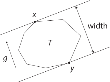
Figure 4. The width of a set $T$ in the direction of $g$.

This reasoning is valid except where we assumed that $g$ is a unit vector. Instead, for $g\sim N(0,I_{n})$ we have $\operatorname{\mathbb{E}}\|g\|_{2}^{2}=n$ and

$$\|g\|_{2}\approx\sqrt{n}\quad\text{with high probability.}$$

(Check both these claims using Bernstein’s inequality.) Thus, we need to scale by the factor $\sqrt{n}$. Ultimately, the geometric interpretation of the Gaussian width becomes the following: $w(T)$ is approximately $\sqrt{n}/2$ larger than the usual, geometric width of $T$ averaged over all directions.

A good exercise is to compute the Gaussian width and complexity for some simple sets, such as the unit balls of the $\ell_{p}$ norms in $\mathbb{R}^{n}$, which we denote $B_{p}^{n}=\{x\in\mathbb{R}^{n}:\;\|x\|_{p}\leq 1\}$. In particular, we have

(61) $$\gamma(B_{2}^{n})\sim\sqrt{n},\quad\gamma(B_{1}^{n})\sim\sqrt{\log n}.$$

For any finite set $T\subset B_{2}^{n}$, we have

(62) $$\gamma(T)\lesssim\sqrt{\log|T|}.$$

The same holds for Gaussian width $w(T)$. (Check these facts!)

A look a these examples reveals that the Gaussian width captures some non-obvious geometric qualities of sets. Of course, the fact that the Gaussian width of the unit Euclidean ball $B_{2}^{n}$ is or order $\sqrt{n}$ is not surprising: the usual, geometric width in all directions is $2$ and the Gaussian width is about $\sqrt{n}$ times that. But it may be surprising that the Gaussian width of the $\ell_{1}$ ball $B_{1}^{n}$ is much smaller, and so is the width of any finite set $T$ (unless the set has exponentially large cardinality). As we will see later, Gaussian width nicely captures the geometric size of “the bulk” of a set.

4.2. Matrix deviation inequality

Now we are ready to answer the question we asked in the beginning of this lecture: what is the magnitude of the uniform deviation (58)? The answer is surprisingly simple: it is bounded by the Gaussian complexity of $T$. The proof is not too simple however, and we will skip it (see the notes after this lecture for references).

Theorem 63 (Matrix deviation inequality).

Let $A$ be an $m\times n$ matrix whose rows $A_{i}$ are independent, isotropic and sub-gaussian random vectors in $\mathbb{R}^{n}$. Let $T\subset\mathbb{R}^{n}$ be a fixed bounded set. Then

$$\operatorname{\mathbb{E}}\sup_{x\in T}\Big{|}\|Ax\|_{2}-\sqrt{m}\|x\|_{2}\Big{|}\leq CK^{2}\gamma(T)$$

where $K=\max_{i}\|A_{i}\|_{\psi_{2}}$ is the maximal sub-gaussian norm of the rows of $A$.

Remark 64 (Tail bound).

It is often useful to have results that hold with high probability rather than in expectation. There exists a high-probability version of the matrix deviation inequality, and it states the following. Let $u\geq 0$. Then the event

(65) $$\sup_{x\in T}\Big{|}\|Ax\|_{2}-\sqrt{m}\|x\|_{2}\Big{|}\leq CK^{2}\left[\gamma(T)+u\cdot\operatorname{rad}(T)\right]$$

holds with probability at least $1-2\exp(-u^{2})$. Here $\operatorname{rad}(T)$ is the radius of $T$, defined as

$$\operatorname{rad}(T):=\sup_{x\in T}\|x\|_{2}.$$

Since $\operatorname{rad}(T)\lesssim\gamma(T)$ (check!) we can continue the bound (65) by

$$\lesssim K^{2}u\gamma(T)$$

for all $u\geq 1$. This is a weaker but still a useful inequality. For example, we can use it to bound all higher moments of the deviation:

(66) $$\Big{(}\operatorname{\mathbb{E}}\sup_{x\in T}\Big{|}\|Ax\|_{2}-\sqrt{m}\|x\|_{2}\Big{|}^{p}\Big{)}^{1/p}\leq C_{p}K^{2}\gamma(T)$$

where $C_{p}\leq C\sqrt{p}$ for $p\geq 1$. (Check this using Proposition 1.)

Remark 67 (Deviation of squares).

It is sometimes helpful to bound the deviation of the square $\|Ax\|_{2}^{2}$ rather than $\|Ax\|_{2}$ itself. We can easily deduce the deviation of squares by using the identity $a^{2}-b^{2}=(a-b)^{2}+2b(a-b)$ for $a=\|Ax\|_{2}$ and $b=\sqrt{m}\|x\|_{2}$. Doing this, we conclude that

(68) $$\operatorname{\mathbb{E}}\sup_{x\in T}\Big{|}\|Ax\|_{2}^{2}-m\|x\|_{2}^{2}\Big{|}\leq CK^{4}\gamma(T)^{2}+CK^{2}\sqrt{m}\operatorname{rad}(T)\gamma(T).$$

(Do this calculation using (66) for $p=2$.) We will use this bound in Section 4.4.

Matrix deviation inequality has many consequences. We will explore some of them now.

4.3. Deriving Johnson-Lindenstrauss Lemma

We started this lecture by promising a result that is more general than Johnson-Lindenstrauss Lemma. So let us show how to quickly derive Johnson-Lindenstrauss from the matrix deviation inequality. Theorem 13 from Theorem 63.

Assume we are in the situation of the Johnson-Lindenstrauss Lemma (Theorem 13). Given a set $\mathcal{X}\subset\mathbb{R}$, consider the normalized difference set

$$T:=\Big{\{}\frac{x-y}{\|x-y\|_{2}}:\;x,y\in\mathcal{X}\text{ distinct vectors}\Big{\}}.$$

Then $T$ is a finite subset of the unit sphere of $\mathbb{R}^{n}$, and thus (62) gives

$$\gamma(T)\lesssim\sqrt{\log|T|}\leq\sqrt{\log|\mathcal{X}|^{2}}\lesssim\sqrt{\log|\mathcal{X}|}.$$

Matrix deviation inequality (Theorem 63) then yields

$$\sup_{x,y\in\mathcal{X}}\Big{|}\frac{\|A(x-y)\|_{2}}{\|x-y\|_{2}}-\sqrt{m}\Big{|}\lesssim\sqrt{\log N}\leq\varepsilon\sqrt{m}.$$

with high probability, say $0.99$. (To pass from expectation to high probability, we can use Markov’s inequality. To get the last bound, we use the assumption on $m$ in Johnson-Lindenstrauss Lemma.)

Multiplying both sides by $\|x-y\|_{2}/\sqrt{m}$, we can write the last bound as follows. With probability at least $0.99$, we have

$$(1-\varepsilon)\|x-y\|_{2}\leq\frac{1}{\sqrt{m}}\|Ax-Ay\|_{2}\leq(1+\varepsilon)\|x-y\|_{2}\quad\text{for all }x,y\in\mathcal{X}.$$

This is exactly the consequence of Johnson-Lindenstrauss lemma.

The argument based on matrix deviation inequality, which we just gave, can be easily extended for infinite sets. It allows one to state a version of Johnson-Lindenstrauss lemma for general, possibly infinite, sets, which depends on the Gaussian complexity of $T$ rather than cardinality. (Try to do this!)

4.4. Covariance estimation

In Section 3.1, we introduced the problem of covariance estimation, and we showed that

$$N\sim n\log n$$

samples are enough to estimate the covariance matrix of a general distribution in $\mathbb{R}^{n}$. We will now show how to do better if the distribution is sub-gaussian. (Recall Section 1.5 for the definition of sub-gaussian random vectors.) In this case, we can get rid of the logarithmic oversampling and the boundedness condition (39).

Theorem 69 (Covariance estimation for sub-gaussian distributions).

Let $X$ be a random vector in $\mathbb{R}^{n}$ with covariance matrix $\Sigma$. Suppose $X$ is sub-gaussian, and more specifically

(70) $$\|\left\langle X,x\right\rangle\|_{\psi_{2}}\lesssim\|\left\langle X,x\right\rangle\|_{L^{2}}=\|\Sigma^{1/2}x\|_{2}\quad\text{for any }x\in\mathbb{R}^{n}.$$

Then, for every $N\geq 1$, we have

$$\operatorname{\mathbb{E}}\|\Sigma_{N}-\Sigma\|\lesssim\|\Sigma\|\;\Big{(}\sqrt{\frac{n}{N}}+\frac{n}{N}\Big{)}.$$

This result implies that if, for $\varepsilon\in(0,1)$, we take a sample of size

$$N\sim\varepsilon^{-2}n,$$

then we are guaranteed covariance estimation with a good relative error:

$$\operatorname{\mathbb{E}}\|\Sigma_{N}-\Sigma\|\leq\varepsilon\|\Sigma\|.$$

Proof.

Since we are going to use Theorem 63, we will need to first bring the random vectors $X,X_{1},\ldots,X_{N}$ to the isotropic position. This can be done by a suitable linear transformation. You will easily check that there exists an isotropic random vector $Z$ such that

$$X=\Sigma^{1/2}Z.$$

(For example, $\Sigma$ has full rank, set $Z:=\Sigma^{-1/2}X$. Check the general case.) Similarly, we can find independent and isotropic random vectors $Z_{i}$ such that

$$X_{i}=\Sigma^{1/2}Z_{i},\quad i=1,\ldots,N.$$

The sub-gaussian assumption (70) then implies that

$$\|Z\|_{\psi_{2}}\lesssim 1.$$

(Check!) Then

$$\|\Sigma_{N}-\Sigma\|=\|\Sigma^{1/2}R_{N}\Sigma^{1/2}\|\quad\text{where}\quad R_{N}:=\frac{1}{N}\sum_{i=1}^{N}Z_{i}Z_{i}^{\mathsf{T}}-I_{n}.$$

The operator norm of a symmetric $n\times n$ matrix $A$ can be computed by maximizing the quadratic form over the unit sphere: $\|A\|=\max_{x\in S^{n-1}}|\left\langle Ax,x\right\rangle|$. (To see this, recall that the operator norm is the biggest eigenvalue of $A$ in magnitude.) Then

$$\|\Sigma_{N}-\Sigma\|=\max_{x\in S^{n-1}}\left\langle\Sigma^{1/2}R_{N}\Sigma^{1/2}x,x\right\rangle=\max_{x\in T}\left\langle R_{N}x,x\right\rangle$$

where $T$ is the ellipsoid

$$T:=\Sigma^{1/2}S^{n-1}.$$

Recalling the definition of $R_{N}$, we can rewrite this as

$$\|\Sigma_{N}-\Sigma\|=\max_{x\in T}\Big{|}\frac{1}{N}\sum_{i=1}^{N}\left\langle Z_{i},x\right\rangle^{2}-\|x\|_{2}^{2}\Big{|}=\frac{1}{N}\max_{x\in T}\big{|}\|Ax\|_{2}^{2}-N\|x\|_{2}^{2}\big{|}.$$

Now we apply the matrix deviation inequality for squares (68) and conclude that

$$\|\Sigma_{N}-\Sigma\|\lesssim\frac{1}{N}\Big{(}\gamma(T)^{2}+\sqrt{N}\operatorname{rad}(T)\gamma(T)\Big{)}.$$

(Do this calculation!) The radius and Gaussian width of the ellipsoid $T$ are easy to compute:

$$\operatorname{rad}(T)=\|\Sigma\|^{1/2}\quad\text{and}\quad\gamma(T)\leq(\operatorname{tr}\Sigma)^{1/2}.$$

Substituting, we get

$$\|\Sigma_{N}-\Sigma\|\lesssim\frac{1}{N}\Big{(}\operatorname{tr}\Sigma+\sqrt{N\|\Sigma\|\operatorname{tr}\Sigma}\Big{)}.$$

To complete the proof, use that $\operatorname{tr}\Sigma\leq n\|\Sigma\|$ (check this!) and simplify the bound. ∎

Remark 71 (Low-dimensional distributions).

Similarly to Section 3.1, we can show that much fewer samples are needed for covariance estimation of low-dimensional sub-gaussian distributions. Indeed, the proof of Theorem 69 actually yields

(72) $$\operatorname{\mathbb{E}}\|\Sigma_{N}-\Sigma\|\leq\|\Sigma\|\;\Big{(}\sqrt{\frac{r}{N}}+\frac{r}{N}\Big{)}$$

where

$$r=r(\Sigma^{1/2})=\frac{\operatorname{tr}\Sigma}{\|\Sigma\|}$$

is the stable rank of $\Sigma^{1/2}$. This means that covariance estimation is possible with

$$N\sim r$$

samples.

4.5. Underdetermined linear equations

We will give one more application of the matrix deviation inequality – this time, to the area of high dimensional inference. Suppose we need to solve a severely underdetermined system of linear equations: say, we have $m$ equations in $n\gg m$ variables. Let us write it in the matrix form as

$$y=Ax$$

where $A$ is a given $m\times n$ matrix, $y\in\mathbb{R}^{m}$ is a given vector and $x\in\mathbb{R}^{n}$ is an unknown vector. We would like to compute $x$ from $A$ and $y$.

When the linear system is underdetermined, we can not find $x$ with any accuracy, unless we know something extra about $x$. So, let us assume that we do have some a-priori information. We can describe this situation mathematically by assuming that

$$x\in K$$

where $K\subset\mathbb{R}^{n}$ is some known set in $\mathbb{R}^{n}$ that describes anything that we know about $x$ a-priori. (Admittedly, we are operating on a high level of generality here. If you need a concrete example, we will consider it in Section 4.6.)

Summarizing, here is the problem we are trying to solve. Determine a solution $x=x(A,y,K)$ to the underdetermined linear equation $y=Ax$ as accurately as possible, assuming that $x\in K$.

A variety of approaches to this and similar problems were proposed during the last decade; see the notes after this lecture for pointers to some literature. The one we will describe here is based on optimization. To do this, it will be convenient to convert the set $K$ into a function on $\mathbb{R}^{n}$ which is called the Minkowski functional of $K$. This is basically a function whose level sets are multiples of $K$. To define it formally, assume that $K$ is star-shaped, which means that together with any point $x$, the set $K$ must contain the entire interval that connects $x$ with the origin; see Figure 5 for illustration. The Minkowski functional of $K$ is defined as

$$\|x\|_{K}:=\inf\big{\{}t>0:\;x/t\in K\big{\}},\quad x\in\mathbb{R}^{n}.$$

If the set $K$ is convex and symmetric about the origin, $\|x\|_{K}$ is actually a norm on $\mathbb{R}^{n}$. (Check this!)

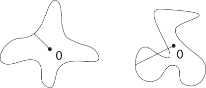
Figure 5. The set on the left (whose boundary is shown) is star-shaped, the set on the right is not.

Now we propose the following way to solve the recovery problem: solve the optimization program

(73) $$\min\|x^{\prime}\|_{K}\quad\text{subject to}\quad y=Ax^{\prime}.$$

Note that this is a very natural program: it looks at all solutions to the equation $y=Ax^{\prime}$ and tries to “shrink” the solution $x^{\prime}$ toward $K$. (This is what minimization of Minkowski functional is about.)

Also note that if $K$ is convex, this is a convex optimization program, and thus can be solved effectively by one of the many available numeric algorithms.

The main question we should now be asking is – would the solution to this program approximate the original vector $x$? The following result bounds the approximation error for a probabilistic model of linear equations. Assume that $A$ is a random matrix as in Theorem 63, i.e. $A$ is an $m\times n$ matrix whose rows $A_{i}$ are independent, isotropic and sub-gaussian random vectors in $\mathbb{R}^{n}$.

Theorem 74 (Recovery by optimization).

The solution $\hat{x}$ of the optimization program (73) satisfies

$$\operatorname{\mathbb{E}}\|\hat{x}-x\|_{2}\lesssim\frac{w(K)}{\sqrt{m}},$$

where $w(K)$ is the Gaussian width of $K$.

Proof.

Both the original vector $x$ and the solution $\hat{x}$ are feasible vectors for the optimization program (73). Then

$$\|\hat{x}\|_{K} \leq\|x\|_{K}\quad\text{(since $\hat{x}$ minimizes the Minkowski functional)}$$

$$\leq 1\quad\text{(since $x\in K$).}$$

Thus both $\hat{x},x\in K$.

We also know that $A\hat{x}=Ax=y$, which yields

(75) $$A(\hat{x}-x)=0.$$

Let us apply matrix deviation inequality (Theorem 63) for $T:=K-K$. It gives

$$\operatorname{\mathbb{E}}\sup_{u,v\in K}\Big{|}\|A(u-v)\|_{2}-\sqrt{m}\,\|u-v\|_{2}\Big{|}\lesssim\gamma(K-K)=2w(K),$$

where we used (60) in the last identity. Substitute $u=\hat{x}$ and $v=x$ here. We may do this since, as we noted above, both these vectors belong to $K$. But then the term $\|A(u-v)\|_{2}$ will equal zero by (75). It disappears from the bound, and we get

$$\operatorname{\mathbb{E}}\sqrt{m}\,\|\hat{x}-x\|_{2}\lesssim w(K).$$

Dividing both sides by $\sqrt{m}$ we complete the proof. ∎

Theorem 74 says that a signal $x\in K$ can be efficiently recovered from

$$m\sim w(K)^{2}$$

random linear measurements.

4.6. Sparse recovery

Let us illustrate Theorem 74 with an important specific example of the feasible set $K$.

Suppose we know that the signal $x$ is sparse, which means that only a few coordinates of $x$ are nonzero. As before, our task is to recover $x$ from the random linear measurements given by the vector

$$y=Ax,$$

where $A$ is an $m\times n$ random matrix. This is a basic example of sparse recovery problems, which are ubiquitous in various disciplines.

The number of nonzero coefficients of a vector $x\in\mathbb{R}^{n}$, or the sparsity of $x$, is often denoted $\|x\|_{0}$. This is similar to the notation for the $\ell_{p}$ norm $\|x\|_{p}=(\sum_{i=1}^{n}|x_{i}|^{p})^{1/p}$, and for a reason. You can quickly check that

(76) $$\|x\|_{0}=\lim_{p\to 0}\|x\|_{p}$$

(Do this!) Keep in mind that neither $\|x\|_{0}$ nor $\|x\|_{p}$ for $0<p<1$ are actually norms on $\mathbb{R}^{n}$, since they fail triangle inequality. (Give an example.)

Let us go back to the sparse recovery problem. Our first attempt to recover $x$ is to try the following optimization problem:

(77) $$\min\|x^{\prime}\|_{0}\quad\text{subject to}\quad y=Ax^{\prime}.$$

This is sensible because this program selects the sparsest feasible solution. But there is an implementation caveat: the function $f(x)=\|x\|_{0}$ is highly non-convex and even discontinuous. There is simply no known algorithm to solve the optimization problem (77) efficiently.

To overcome this difficulty, let us turn to the relation (76) for an inspiration. What if we replace $\|x\|_{0}$ in the optimization problem (77) by $\|x\|_{p}$ with $p>0$? The smallest $p$ for which $f(x)=\|x\|_{p}$ is a genuine norm (and thus a convex function on $\mathbb{R}^{n}$) is $p=1$. So let us try

(78) $$\min\|x^{\prime}\|_{1}\quad\text{subject to}\quad y=Ax^{\prime}.$$

This is a convexification of the non-convex program (77), and a variety of numeric convex optimization methods are available to solve it efficiently.

We will now show that $\ell_{1}$ minimization works nicely for sparse recovery. As before, we assume that $A$ is a random matrix as in Theorem 63.

Theorem 79 (Sparse recovery by optimization).

Assume that an unknown vector $x\in\mathbb{R}^{n}$ has at most $s$ non-zero coordinates, i.e. $\|x\|_{0}\leq s$. The solution $\hat{x}$ of the optimization program (78) satisfies

$$\operatorname{\mathbb{E}}\|\hat{x}-x\|_{2}\lesssim\sqrt{\frac{s\log n}{m}}\;\|x\|_{2}.$$

Proof.

Since $\|x\|_{0}\leq s$, Cauchy-Schwarz inequality shows that

(80) $$\|x\|_{1}\leq\sqrt{s}\,\|x\|_{2}.$$

(Check!) Denote the unit ball of the $\ell_{1}$ norm in $\mathbb{R}^{n}$ by $B_{1}^{n}$, i.e. $B_{1}^{n}:=\{x\in\mathbb{R}^{n}:\;\|x\|_{1}\leq 1\}$. Then we can rewrite (80) as the inclusion

$$x\in\sqrt{s}\,\|x\|_{2}\cdot B_{1}^{n}:=K.$$

Apply Theorem 74 for this set $K$. We noted the Gaussian width of $B_{1}^{n}$ in (61), so

$$w(K)=\sqrt{s}\,\|x\|_{2}\cdot w(B_{1}^{n})\leq\sqrt{s}\,\|x\|_{2}\cdot\gamma(B_{1}^{n})\leq\sqrt{s}\,\|x\|_{2}\cdot\sqrt{\log n}.$$

Substitute this in Theorem 74 and complete the proof. ∎

Theorem 79 says that an $s$-sparse signal $x\in\mathbb{R}^{n}$ can be efficiently recovered from

$$m\sim s\log n$$

random linear measurements.

4.7. Notes

For a more thorough introduction to Gaussian width and its role in high-dimensional estimation, refer to the tutorial [59] and the textbook [60]; see also [5]. Related to Gaussian complexity is the notion of Rademacher complexity of $T$, obtained by replacing the coordinates of $g$ by independent Rademacher (i.e. $\pm 1$ symmetric) random variables. Rademacher complexity of classes of functions plays an important role in statistical learning theory, see e.g. [44]

Matrix deviation inequality (Theorem 63) is borrowed from [41]. In the special case where $A$ is a Gaussian random matrix, this result follows from the work of G. Schechtman [57] and could be traced back to results of Gordon [24, 25, 26, 27].

In the general case of sub-gaussian distributions, earlier variants of Theorem 63 were proved by B. Klartag and S. Mendelson [35], S. Mendelson, A. Pajor and N. Tomczak-Jaegermann [45] and S. Dirksen [20].

Theorem 69 for covariance estimation can be proved alternatively using more elementary tools (Bernstein’s inequality and $\varepsilon$-nets), see [58]. However, no known elementary approach exists for the low-rank covariance estimation discussed in Remark 71. The bound (72) was proved by V. Koltchinskii and K. Lounici [36] by a different method.

In Section 4.5, we scratched the surface of a recently developed area of sparse signal recovery, which is also called compressed sensing. Our presentation there essentially follows the tutorial [59]. Theorem 79 can be improved: if we take

$$m\gtrsim s\log(n/s)$$

measurements, then with high probability the optimization program (78) recovers the unknown signal $x$ exactly, i.e.

$$\hat{x}=x.$$

First results of this kind were proved by J. Romberg, E. Candes and T. Tao [13] and a great number of further developments followed; refer e.g. to the book [23] and the chapter in [19] for an introduction into this research area.

References

- [1] E. Abbe, A. S. Bandeira, G. Hall. Exact recovery in the stochastic block model, IEEE Transactions on Information Theory 62 (2016), 471–487.
- [2] D. Achlioptas, Database-friendly random projections: Johnson-Lindenstrauss with binary coins, Journal of Computer and System Sciences, 66 (2003), 671–687.
- [3] R. Ahlswede, A. Winter, Strong converse for identification via quantum channels, IEEE Trans. Inf. Theory 48 (2002), 569–579.
- [4] N. Ailon, B. Chazelle, Approximate nearest neighbors and the fast Johnson-Lindenstrauss transform, Proceedings of the 38th Annual ACM Symposium on Theory of Computing. New York: ACM Press, 2006. pp. 557–563.
- [5] D. Amelunxen, M. Lotz, M. McCoy, J. Tropp, Living on the edge: phase transitions in convex programs with random data, Inf. Inference 3 (2014), 224–294.
- [6] A. Bandeira, R. van Handel, Sharp nonasymptotic bounds on the norm of random matrices with independent entries, Ann. Probab. 44 (2016), 2479–2506.
- [7] R. Baraniuk, M. Davenport, R. DeVore, M. Wakin, A simple proof of the restricted isometry property for random matrices, Constructive Approximation, 28 (2008), 253–263.
- [8] R. Bhatia, Matrix Analysis. Graduate Texts in Mathematics, vol. 169. Springer, Berlin, 1997.
- [9] C. Bordenave, M. Lelarge, L. Massoulie, |em Non-backtracking spectrum of random graphs: community detection and non-regular Ramanujan graphs, Annals of Probability, to appear.
- [10] S. Boucheron, G. Lugosi, P. Massart, Concentration inequalities. A nonasymptotic theory of independence. With a foreword by Michel Ledoux. Oxford University Press, Oxford, 2013.
- [11] O. Bousquet1, S. Boucheron, G. Lugosi, Introduction to statistical learning theory, in: Advanced Lectures on Machine Learning, Lecture Notes in Computer Science 3176, pp.169–207, Springer Verlag 2004.
- [12] T. Cai, R. Zhao, H. Zhou, Estimating structured high-dimensional covariance and precision matrices: optimal rates and adaptive estimation, Electron. J. Stat. 10 (2016), 1–59.
- [13] E. Candes, J. Romberg, T. Tao, Robust uncertainty principles: exact signal reconstruction from highly incomplete frequency information, IEEE Trans. Inform. Theory 52 (2006), 489–509.
- [14] E. Candes, B. Recht, Exact Matrix Completion via Convex Optimization, Foundations of Computational Mathematics 9 (2009), 717–772.
- [15] E. Candes, T. Tao, The power of convex relaxation: near-optimal matrix completion, IEEE Trans. Inform. Theory 56 (2010), 2053–2080.
- [16] R. Chen, A. Gittens, J. Tropp, The masked sample covariance estimator: an analysis using matrix concentration inequalities, Inf. Inference 1 (2012), 2–20.
- [17] P. Chin, A. Rao, and V. Vu, |em Stochastic block model and community detection in the sparse graphs: A spectral algorithm with optimal rate of recovery, preprint, 2015.
- [18] M. Davenport, Y. Plan, E. van den Berg, M. Wootters, 1-bit matrix completion, Inf. Inference 3 (2014), 189–223.
- [19] M. Davenport, M. Duarte, Yonina C. Eldar, Gitta Kutyniok, Introduction to compressed sensing, in: Compressed sensing. Edited by Yonina C. Eldar and Gitta Kutyniok. Cambridge University Press, Cambridge, 2012.
- [20] S. Dirksen, Tail bounds via generic chaining, Electron. J. Probab. 20 (2015), 1–29.
- [21] U. Feige, E. Ofek, Spectral techniques applied to sparse random graphs, Random Structures Algorithms 27 (2005), 251–275.
- [22] S. Fortunato, Santo; D. Hric, Community detection in networks: A user guide. Phys. Rep. 659 (2016), 1–44.
- [23] S. Foucart, H. Rauhut, A mathematical introduction to compressive sensing. Applied and Numerical Harmonic Analysis. Birkhäuser/Springer, New York, 2013.
- [24] Y. Gordon, Some inequalities for Gaussian processes and applications, Israel J. Math. 50 (1985), 265–289.
- [25] Y. Gordon, Elliptically contoured distributions, Prob. Th. Rel. Fields 76 (1987), 429–438.
- [26] Y. Gordon, On Milman’s inequality and random subspaces which escape through a mesh in , Geometric aspects of functional analysis (1986/87), Lecture Notes in Math., vol. 1317, pp. 84–106.
- [27] Y. Gordon, Majorization of Gaussian processes and geometric applications, Prob. Th. Rel. Fields 91 (1992), 251–267.
- [28] D. Gross, Recovering low-rank matrices from few coefficients in any basis, IEEE Trans. Inform. Theory 57 (2011), 1548–1566.
- [29] O. Guedon, R. Vershynin, Community detection in sparse networks via Grothendieck’s inequality, Probability Theory and Related Fields 165 (2016), 1025–1049.
- [30] A. Javanmard, A. Montanari, F. Ricci-Tersenghi, Phase transitions in semidefinite relaxations, PNAS, April 19, 2016, vol. 113, no.16, E2218–E2223.
- [31] W. B. Johnson, J. Lindenstrauss, Extensions of Lipschitz mappings into a Hilbert space. In Beals, Richard; Beck, Anatole; Bellow, Alexandra; et al. Conference in modern analysis and probability (New Haven, Conn., 1982). Contemporary Mathematics. 26. Providence, RI: American Mathematical Society, 1984. pp. 189–206.
- [32] B. Hajek, Y. Wu, J. Xu, Achieving exact cluster recovery threshold via semidefinite programming, IEEE Transactions on Information Theory 62 (2016), 2788–2797.
- [33] P. W. Holland, K. B. Laskey, S. Leinhardt, |em Stochastic blockmodels: first steps, Social Networks 5 (1983), 109–137.
- [34] D. Kane, J. Nelson, Sparser Johnson-Lindenstrauss Transforms, Journal of the ACM 61 (2014): 1.
- [35] B. Klartag, S. Mendelson, Empirical processes and random projections, J. Funct. Anal. 225 (2005), 229–245.
- [36] V. Koltchinskii, K. Lounici, Concentration inequalities and moment bounds for sample covariance operators, Bernoulli 23 (2017), 110–133.
- [37] C. Le, E. Levina, R. Vershynin, Concentration and regularization of random graphs, Random Structures and Algorithms, to appear.
- [38] M. Ledoux, The concentration of measure phenomenon. American Mathematical Society, Providence, RI, 2001.
- [39] M. Ledoux, M. Talagrand, Probability in Banach spaces. Isoperimetry and processes. Springer-Verlag, Berlin, 1991.
- [40] E. Levina, R. Vershynin, Partial estimation of covariance matrices, Probability Theory and Related Fields 153 (2012), 405–419.
- [41] C. Liaw, A. Mehrabian, Y. Plan, R. Vershynin, A simple tool for bounding the deviation of random matrices on geometric sets, Geometric Aspects of Functional Analysis, Lecture Notes in Mathematics, Springer, Berlin, to appear.
- [42] J. Matou ek, Lectures on discrete geometry. Graduate Texts in Mathematics, 212. Springer-Verlag, New York, 2002.
- [43] F. McSherry, Spectral partitioning of random graphs, Proc. 42nd FOCS (2001), 529–537.
- [44] S.Mendelson,S.Mendelson, A few notes on statistical learning theory, in: Advanced Lectures on Machine Learning, S. Mendelson, A.J. Smola (Eds.) LNAI 2600, pp. 1–40, 2003.
- [45] S. Mendelson, A. Pajor, N. Tomczak-Jaegermann, Reconstruction and subgaussian operators in asymptotic geometric analysis. Geom. Funct. Anal. 17 (2007), 1248–1282.
- [46] E. Mossel, J. Neeman, A. Sly, Belief propagation, robust reconstruction and optimal recovery of block models. Ann. Appl. Probab. 26 (2016), 2211–2256.
- [47] M. E. Newman, Networks. An introduction. Oxford University Press, Oxford, 2010.
- [48] R. I. Oliveira, Concentration of the adjacency matrix and of the Laplacian in random graphs with independent edges, unpublished (2010), arXiv:0911.0600.
- [49] R. I. Oliveira, Sums of random Hermitian matrices and an inequality by Rudelson, Electron. Commun. Probab. 15 (2010), 203–212.
- [50] Y. Plan, R. Vershynin, E. Yudovina, High-dimensional estimation with geometric constraints, Information and Inference 0 (2016), 1–40.
- [51] S. Riemer, C. Schütt, On the expectation of the norm of random matrices with non-identically distributed entries, Electron. J. Probab. 18 (2013), no. 29, 13 pp.
- [52] J. Tropp, User-friendly tail bounds for sums of random matrices. Found. Comput. Math. 12 (2012), 389–434.
- [53] J. Tropp, An introduction to matrix concentration inequalities. Found. Trends Mach. Learning 8 (2015), 10-230.
- [54] R. van Handel, Structured random matrices. in: IMA Volume “Discrete Structures: Analysis and Applications”, Springer, to appear.
- [55] R. van Handel, On the spectral norm of Gaussian random matrices, Trans. Amer. Math. Soc., to appear.
- [56] B. Recht, A simpler approach to matrix completion, J. Mach. Learn. Res. 12 (2011), 3413–3430.
- [57] G. Schechtman, Two observations regarding embedding subsets of Euclidean spaces in normed spaces, Adv. Math. 200 (2006), 125–135.
- [58] R. Vershynin, Introduction to the non-asymptotic analysis of random matrices. Compressed sensing, 210–268, Cambridge University Press, Cambridge, 2012.
- [59] R. Vershynin, Estimation in high dimensions: a geometric perspective. Sampling Theory, a Renaissance, 3–66, Birkhauser Basel, 2015.
- [60] R. Vershynin, High-Dimensional Probability. An Introduction with Applications in Data Science. Cambridge University Press, to appear.
- [61] H. Zhou, A. Zhang, Minimax Rates of Community Detection in Stochastic Block Models, Annals of Statistics, to appear.