One-dimensional Modelling of Electrostatic Generation and Detection of Bulk Acoustic Waves in layered structures

Abstract

This paper is devoted to the unidimensional analysis of a 2-ports silicon resonator vibrating in thickness–extensional mode. Both excitation and detection ports are capacitive transducers used to control the system of longitudinal elastic waves established along the thickness of a layered structure. The analysis consists of integrating the capacitive transduction of longitudinal elastic waves within a specific implementation of the general scheme of impedance methods largely used as standard tools for the modelling of RF-MEMS.

1 Position of problem

This short paper is devoted to the one–dimensional analysis of a silicon resonator vibrating in thickness–extensional mode with a 2–ports capacitive system for excitation and detection of the elastic waves. The device under study is schematically represented on Fig. 1.

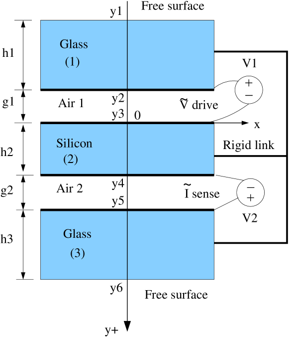
Figure 1: Schematic view of the structure under study.

The three layers of solid materials form a rigid assembly, leaving thin gaps $g_{1}$ and $g_{2}$ between the pairs of inner interfaces. Throughout the paper, we use bars and tilde to denote static and dynamic quantities, respectively. With these conventions, a driving voltage

$$V_{1}=\overline{V}_{1}+\widetilde{V}_{1}\cos\omega t$$ (1)

is applied across the first air gap (input port 1), whereas a purely static voltage $V_{2}\equiv\overline{V}_{2}$ is applied across the second air gap (output port 2). The thickness of the layered structure is oriented along the second axis $\vec{y}$ axis of the frame. The extension of the stacked structure along $\vec{x}$ and $\vec{z}$ is assumed large enough to justify the one-dimensionnal assumption, i.e. all quantities of interest only depend on the $y$ coordinate. Each air-solid inner interface is coated with an infinitely thin conductive electrode, and the thickness $h_{2}$ of the silicon layer is considered sufficient to neglect electrostatic influence between the electrodes located at $y_{3}$ and $y_{4}$.

Here-proposed analysis essentially follows a specific implementation of the general scheme of the impedance matrices approach [1], widely used to describe linear problems in the domains of ultrasonics and piezoelectricity. Since electrostatic excitation of MEMS devices is intrinsically non–linear, the very first step must consist in linearizing the excitation problem around the static bias point imposed by $\overline{V}_{1}$ and $\overline{V}_{2}$ prior integrating the whole problem within the formalism of laminar plate Green’s functions closely related to acoustic admittance matrices. The instantaneous value of the net electrostatic surface force is given by:

$$\vec{f}_{e}(t)=\frac{\varepsilon_{0}}{2}\,\frac{\left[{V_{1}(t)}\right]^{2}}{\left[g_{1}-u_{2}(y_{2})+u_{2}(y_{3})\right]^{2}}\,\vec{n},$$ (2)

where $u_{2}$ denotes the total (static + dynamic) out-of-plane component of the mechanical displacement along the interface, and $\vec{n}$ is the unit normal to the considered interface, outwardly oriented with respect to the solid. Since no fringing effect can be accounted for in the framework of the purely unidimensionnal analysis, the thickness extensional stress is identical on both sides of the thin electrostatic gap. With present notations, one obtains:

$$T_{2}(y_{2})=T_{2}(y_{3})=\frac{\varepsilon_{0}}{2}\frac{{V_{0}}^{2}+2\overline{V}_{1}\widetilde{V}_{1}\cos\omega t+\frac{{\widetilde{V}_{1}}^{2}}{2}\cos 2\omega t}{\left(g_{1}+u_{32}\right)^{2}},$$ (3)

where we introduced the notations:

$$\begin{array}[]{ccc}{V_{0}}=\sqrt{{\overline{V}_{1}}^{2}+\frac{{\widetilde{V}_{1}}^{2}}{2}}&\mbox{ and }&u_{32}=u_{2}(y_{3})-u_{2}(y_{2}).\end{array}$$ (4)

Using similar notations, the extensional stress on both banks of the capacitive transducer of port 2 is given by a simpler expression since the bias voltage $V_{2}$ applied to that port is constant:

$$T_{2}(y_{4})=T_{2}(y_{5})=\frac{\varepsilon_{0}}{2}\frac{{\overline{V}_{2}}^{2}}{\left(g_{2}+u_{54}\right)^{2}}$$ (5)

with

$$u_{54}=u_{2}(y_{5})-u_{2}(y_{4}).$$ (6)

At any point along the thickness of the layered structure, the normal displacement can be split into static and dynamic parts:

$$u_{2}(y,t)=\bar{u}_{2}(y)+\tilde{u}_{2}(y,t).$$ (7)

Furthermore, let us restrict our attention to the case $\widetilde{V}_{1}\ll\overline{V}_{1}$ at the input port. Then we can drop the second harmonic term ($\cos 2\omega t$) in (3). As long as the biasing voltage stays smaller than the pull–in threshold [2] in both gaps, causality and visco-elastic damping ruling the propagation of elastic waves in solids permit us to consider that the dynamic displacement is small but not negligible with respect to the finite dimensions of the biased structure, including the small gaps. Then the dynamic component of the mechanical strain and stress of interest, $S_{2}$ and $T_{2}$, respectively, remain infinitesimal in the entire structure, so that we can linearize the solution of the complete problem around its static solution:

$$\begin{array}[]{l}\tilde{S}_{2}(y,t)=\lim_{\tilde{V}_{1}/\bar{V}_{1}\rightarrow 0}\left(S_{2}(y,t)-\bar{S}_{2}(y)\right),\vspace{0.6em}\\ \tilde{T}_{2}(y,t)=\lim_{\tilde{V}_{1}/\bar{V}_{1}\rightarrow 0}\left(T_{2}(y,t)-\bar{T}_{2}(y)\right).\end{array}$$ (8)

Applying this procedure we obtain the following first-order expansions of the dynamic extensional stress at all interfaces of the structure:

$$\begin{array}[]{l}\widetilde{T}_{2}(y_{1},t)=0,\vspace{0.6em}\\ \displaystyle\widetilde{T}_{2}(y_{2},t)=\widetilde{T}_{2}(y_{3},t)=\varepsilon_{0}\left[\frac{\overline{V}_{1}\widetilde{V}_{1}\cos\omega t}{\left(g_{1}+\bar{u}_{32}\right)^{2}}-\frac{{V_{0}}^{2}\,\tilde{u}_{32}(t)}{\left(g_{1}+\bar{u}_{32}\right)^{3}}\right],\vspace{0.6em}\\ \displaystyle\widetilde{T}_{2}(y_{4},t)=\widetilde{T}_{2}(y_{5},t)=-\frac{\varepsilon_{0}{\overline{V}_{2}}^{2}\,\tilde{u}_{54}(t)}{\left(g_{2}+\bar{u}_{54}\right)^{3}},\vspace{0.6em}\\ \displaystyle\widetilde{T}_{2}(y_{6},t)=0.\end{array}$$ (9)

2 Solution by Green’s function treatment

The system of Eqs. (9) establishes a useful relationship between stresses, normal displacement and electric potential at all interfaces of the structure. Its linearity permits the use of the complex notation. Denoting the complex amplitudes of $\widetilde{T}_{2}(y_{i},t)$ and $\tilde{u}_{2}(y_{i},t)$ by $\tau_{i}$ and $\upsilon_{i}$, respectively, we easily turn (9) into a quite systematic form:

$$\left[\begin{array}[]{c}\tau_{1}\\ \tau_{2}\\ \tau_{3}\\ \tau_{4}\\ \tau_{5}\\ \tau_{6}\end{array}\right]=\left[\begin{array}[]{c}0\\ K\widetilde{V}_{1}\\ K\widetilde{V}_{1}\\ 0\\ 0\\ 0\end{array}\right]+\left[\begin{array}[]{cccccc}0&0&0&0&0&0\\ 0&L&-L&0&0&0\\ 0&L&-L&0&0&0\\ 0&0&0&M&-M&0\\ 0&0&0&M&-M&0\\ 0&0&0&0&0&0\end{array}\right]\left[\begin{array}[]{c}\upsilon_{1}\\ \upsilon_{2}\\ \upsilon_{3}\\ \upsilon_{4}\\ \upsilon_{5}\\ \upsilon_{6}\end{array}\right]$$ (10)

where:

$$\begin{array}[]{ccc}\displaystyle K=\frac{\varepsilon_{0}\overline{V}_{1}}{\left(g_{1}+\bar{u}_{32}\right)^{2}},&\displaystyle L=\frac{\varepsilon_{0}{V_{0}}^{2}}{\left(g_{1}+\bar{u}_{32}\right)^{3}},&\displaystyle M=\frac{\varepsilon_{0}{\overline{V}_{2}}^{2}}{\left(g_{2}+\bar{u}_{54}\right)^{2}}.\end{array}$$ (11)

The well-known theory of plane waves propagation along a given axis of a purely elastic solid permits to state the existence of definite transfer matrices for the acoustic propagation in all elastic layers of the structure[3]. In here-considered structure, we only consider cubic or isotropic solids. Then, the transfer matrices of interest are of dimensions $[2\times 2]$, as well as the acoustic impedance or admittance matrices and Green’s functions related to them[4]. Thus, the admittance form of Green’s function matrix[5] of the considered laminar plate forming the layer $(n)$ is well defined, according to the procedure summarized in the Appendix:

$$\left[\begin{array}[]{c}\upsilon_{(2n-1)}\vspace{0.6em}\\ \upsilon_{(2n)}\end{array}\right]=\left[\begin{array}[]{cc}G_{11}^{(n)}&G_{12}^{(n)}\vspace{0.6em}\\ G_{21}^{(n)}&G_{22}^{(n)}\end{array}\right]\left[\begin{array}[]{c}\tau_{(2n-1)}\vspace{0.6em}\\ \tau_{(2n)}\end{array}\right]$$ (12)

Accordingly, a simple assembly of the matrices obtained for the separate layers provides the detailed form of the Green’s function matrix characterizing the entire structure:

$$\left[\begin{array}[]{c}\upsilon_{1}\vspace{0.5em}\\ \upsilon_{2}\vspace{0.5em}\\ \upsilon_{3}\vspace{0.5em}\\ \upsilon_{4}\vspace{0.5em}\\ \upsilon_{5}\vspace{0.5em}\\ \upsilon_{6}\end{array}\right]=\left[\begin{array}[]{cccccc}G^{(1)}_{11}&G^{(1)}_{12}&0&0&0&0\vspace{0.4em}\\ G^{(1)}_{21}&G^{(1)}_{22}&0&0&0&0\vspace{0.4em}\\ 0&0&G^{(2)}_{11}&G^{(2)}_{12}&0&0\vspace{0.4em}\\ 0&0&G^{(2)}_{21}&G^{(2)}_{22}&0&0\vspace{0.4em}\\ 0&0&0&0&G^{(3)}_{11}&G^{(3)}_{12}\vspace{0.4em}\\ 0&0&0&0&G^{(3)}_{21}&G^{(3)}_{22}\end{array}\right]\left[\begin{array}[]{c}\tau_{1}\vspace{0.5em}\\ \tau_{2}\vspace{0.5em}\\ \tau_{3}\vspace{0.5em}\\ \tau_{4}\vspace{0.5em}\\ \tau_{5}\vspace{0.5em}\\ \tau_{6}\end{array}\right].$$ (13)

Substituting (13) into (10) yields a closed–form solution of the problem through basic linear algebra:

$$\vec{\bm{\upsilon}}=\left[{\bf I}_{(6\times 6)}-{\bf G}_{(6\times 6)}{\bf P}_{(6\times 6)}\right]^{-1}{\bf G}_{(6\times 6)}\left[\begin{array}[]{c}0\\ K\widetilde{V}_{1}\\ K\widetilde{V}_{1}\\ 0\\ 0\\ 0\end{array}\right]$$ (14)

where ${\bf G}_{(6\times 6)}$ is the $6\times 6$ matrix appearing in (13), ${\bf I}$ denotes the identity matrix, and ${\bf P}$ is the $6\times 6$ matrix appearing in the right hand member of (10).

3 Electrical response

Figure 2: Electrical representation of the studied structure.

Electromechanical analogies are frequently performed to model the MEMS resonators via equivalent electrical circuits [6]. Here-proposed approach permits to directly access the electrical response of thickness–extensional modes in stacked structures.

Let us assume that the silicon layer is electrically grounded. Then the device is an electrical quadripole as shown on Fig. 2. The charge borne by the output electrode at $y_{5}$ is easily obtained from Gauss’ theorem:

$$q=\varepsilon_{0}\int_{S}n_{2}E_{2}\,dS=-\varepsilon_{0}\int_{S}E_{2}\,dS.$$ (15)

The corresponding current delivered by the constant voltage source $\overline{V}_{2}$ to that electrode is:

$$I=\dot{q}=\varepsilon_{0}\overline{V}_{2}\int_{S}\frac{\partial}{\partial t}\left(\frac{1}{g_{2}+\bar{u}_{54}+\tilde{u}_{54}}\right)\,dS.$$ (16)

Performing a Taylor’s expansion of the locally–deformed gap with respect to the small incremental dynamic variation, one obtains the corresponding current, with the notations used throughout this paper

$$I\approx j\omega\varepsilon_{0}\overline{V}_{2}\int_{S}\frac{\upsilon_{4}-\upsilon_{5}}{\left(g_{2}+\bar{u}_{54}\right)^{2}}\,dS.$$ (17)

Then, the current is easily derived from the displacement solution established in (14).

4 Application

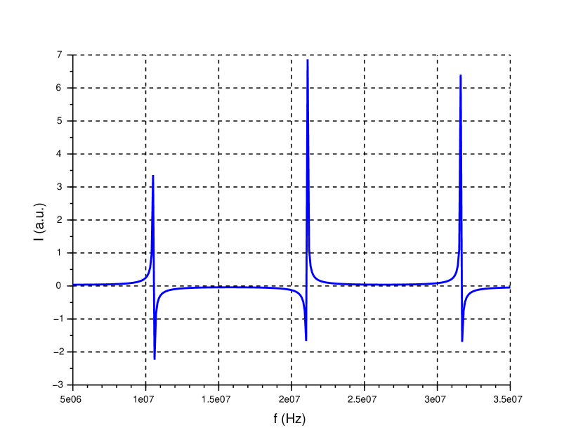
Figure 3: Computed imaginary part of current $Im(I)(\tilde{V}_{1})$ in the output port in terms of frequency.

Fig. 3 shows a plot of the current in the output port in terms of frequency, for the following parameters: $h^{(1)}=h^{(3)}=1\,mm$, $h^{(2)}=400\;\mu m$, $\overline{V}_{1}=\overline{V}_{2}=100\,V$, $\tilde{V}_{1}=1\,V$. One observes little influence of the resonances of the bottom layer (glass) onto the current output. For comparison, we provide on Fig. 4 a plot of the current delivered by the source at the input port. In that case, the contribution of vibration of the bottom glass wafer is clearly visible.

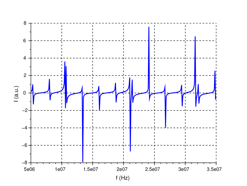
Figure 4: Computed imaginary part of the current $Im(I)(\tilde{V}_{1})$ in the input port in terms of frequency.

Since electrostatic driving is actually performed by an external mechanical force, either even and odd modes can be driven through the two-ports setup sown on Fig. 1. This also explains that the behavior of the phase observed on Fig. 3 is different from the behavior that would be observed upon operating thickness modes in a stack of solid layers with help of some piezoelectric layer, for instance. This ability to drive both symmetric and antismmetric modes is easily confirmed by analyzing the frequency dependence of the vector of mechanical displacements at all interfaces, provided by Eq. (14).

Acknowldegements

This work has been partially supported through the MEMS-RF project of the Laboratory of Excellence FIRST-TF.

Appendix A Detailed form of required matrices

A combination of longitudinal plane waves propagating along both positive and negative directions of $\vec{x}_{2}$ axis in one of the solid layer of the structure is represented by:

$$\tilde{u}_{2}(y)=\left(A^{+}e^{-j\omega sy}+A^{-}e^{j\omega sy}\right)\,e^{j\omega t}$$ (18)

where $s$ denotes the slowness of the elastic waves in the direction of interest.Then the longitudinal stress created by this elastic wave is given by:

$$\widetilde{T}_{2}(y)=-j\omega Z\left(A^{+}e^{-j\omega sy}-A^{-}e^{j\omega sy}\right)\,e^{j\omega t},$$ (19)

where $Z=\sqrt{\rho c_{22}}$ is the acoustic impedance of the layer, $c_{22}$ being the elastic constant ruling the propagation along the considered axis, and $\rho$ is the mass density of the layer.

Let $(n)$ denote this layer. The identification of $\tilde{u}_{2}$ and $\widetilde{T}_{2}$ at the coordinate $y_{2n-1}$ in the notations of this paper permits to obtain $A^{+}$ and $A^{-}$. Then a second identification of $\tilde{u}_{2}$ and $\widetilde{T}_{2}$ at the other end of the layer, i.e. $y_{2n}$ straightforwardly gives the expression of the transfer matrix between both surfaces of the said layer. With present notations, the forward transfer matrix, defined by

$$\left[\begin{array}[]{c}\upsilon_{(2n)}\vspace{0.4em}\\ \tau_{(2n)}\end{array}\right]={\bm{M}^{(n)}}\left[\begin{array}[]{c}\upsilon_{(2n-1)}\vspace{0.4em}\\ \tau_{(2n-1)}\end{array}\right]$$ (20)

has the following expressions:

$${\bm{M}^{(n)}}=\left[\begin{array}[]{cc}\displaystyle\cos\omega s^{(n)}h_{n}&\displaystyle\frac{\sin\omega s^{(n)}h_{n}}{Z^{(n)}\omega}\vspace{0.6em}\\ \displaystyle-Z^{(n)}\omega\sin\omega s^{(n)}h_{n}&\displaystyle\cos\omega s^{(n)}h_{n}\end{array}\right],\vspace{0.4em}$$ (21)

where the slowness $s^{(n)}$ of the wave in the solid layer $(n)$ is equal to $\sqrt{\rho/c_{22}^{(n)}}$. The backwards transfer matrix is defined by

$$\left[\begin{array}[]{c}\upsilon_{(2n)}\vspace{0.4em}\\ \tau_{(2n)}\end{array}\right]={\bm{N}^{(n)}}\left[\begin{array}[]{c}\upsilon_{(2n-1)}\vspace{0.4em}\\ \tau_{(2n-1)}\end{array}\right]$$ (22)

and ${\bm{N}^{(n)}}=\left(\bm{M}^{(n)}\right)^{-1}$ is actually equal to the transpose of $\bm{M}^{(n)}$ since $\mbox{det}({\bm{M}})=1$:

$${\bm{N}^{(n)}}=\left[\begin{array}[]{cc}\displaystyle\cos\omega s^{(n)}h_{n}&\displaystyle-\frac{\sin\omega s^{(n)}h_{n}}{Z^{(n)}\omega}\vspace{0.6em}\\ \displaystyle Z^{(n)}\omega\sin\omega s^{(n)}h_{n}&\displaystyle\cos\omega s^{(n)}h_{n}\end{array}\right].$$ (23)

The admittance form expression of Green’s function matrix of the considered laminar layer is defined by [5]:

$$\left[\begin{array}[]{c}\upsilon_{(2n-1)}\vspace{0.4em}\\ \upsilon_{(2n)}\end{array}\right]={\bm{G}^{(n)}}\left[\begin{array}[]{c}\tau_{(2n-1)}\vspace{0.4em}\\ \tau_{(2n)}\end{array}\right].$$ (24)

Basic matrix operations permit to obtain the elements of $\bm{G}^{(n)}$ from (23):

$${\bm{G}^{(n)}}=\left[\begin{array}[]{lc}\displaystyle{\frac{N_{11}^{(n)}}{N_{21}^{(n)}}}&\displaystyle N^{(n)}_{12}-\frac{N^{(n)}_{11}N^{(n)}_{22}}{N^{(n)}_{21}}\vspace{0.4em}\\ \displaystyle\frac{1}{N^{(n)}_{21}}&\displaystyle-\frac{N^{(n)}_{22}}{N^{(n)}_{21}}\end{array}\right].$$ (25)

References

• [1] W. P. Mason. Physical Acoustics and the properties of solid. D. Van Nostrand, Princeton, NJ, 1958.
• [2] R. A . Wickstrom H. Nathanson, W. E. Newell and J. R. Davis Jr. The resonant gate transistor. IEEE Trans. Electron Devices, ED-14:157–176, 1996.
• [3] A. H. Fahmy and E. Adler. Propagation of surface acoustic waves in multilayer: a matrix description. Appl. Phys. Lett., (22):495–497, 1973.
• [4] P. M. Smith. Dyadic Green’s function for multi-layer SAW substrates. IEEE Trans. on Ultrasonics, Ferroelectrics and Frequency Control, 48(1):171–179, 2001.
• [5] A. Khelif A. Reinhardt, V. Laude and S. Ballandras. Dyadic Green’s Function of a Laminar Plate. IEEE Trans. on Ultrasonics, Ferroelectrics and Frequency Control, 51(9):1157–1163, 2004.
• [6] J. R. Clark F. D. Bannon, III and T.-C. Nguyen. High-Q HF Microelectromechanical Filters. IEEE Journal of Solid-state circuits, 35(4):512–526, 2000.