Exploring Different Dimensions of Attention for Uncertainty Detection

Abstract

Neural networks with attention have proven effective for many natural language processing tasks. In this paper, we develop attention mechanisms for uncertainty detection. In particular, we generalize standardly used attention mechanisms by introducing external attention and sequence-preserving attention. These novel architectures differ from standard approaches in that they use external resources to compute attention weights and preserve sequence information. We compare them to other configurations along different dimensions of attention. Our novel architectures set the new state of the art on a Wikipedia benchmark dataset and perform similar to the state-of-the-art model on a biomedical benchmark which uses a large set of linguistic features.

1 Introduction

For many natural language processing (NLP) tasks, it is essential to distinguish uncertain (non-factual) from certain (factual) information. Such tasks include information extraction, question answering, medical information retrieval, opinion detection, sentiment analysis [Karttunen and Zaenen (2005, Vincze (2014a, Díaz et al. (2016] and knowledge base population (KBP). In KBP, we need to distinguish, e.g., “X may be Basque” and “X was rumored to be Basque” (uncertain) from “X is Basque” (certain) to decide whether to add the fact “Basque(X)” to a knowledge base. In this paper, we use the term uncertain information to refer to speculation, opinion, vagueness and ambiguity. We focus our experiments on the uncertainty detection (UD) dataset from the CoNLL2010 hedge cue detection task [Farkas et al. (2010]. It consists of two medium-sized corpora from different domains (Wikipedia and biomedical) that allow us to run a large number of comparative experiments with different neural networks and exhaustively investigate different dimensions of attention.

Convolutional and recurrent neural networks (CNNs and RNNs) perform well on many NLP tasks [Collobert et al. (2011, Kalchbrenner et al. (2014, Zeng et al. (2014, Zhang and Wang (2015]. CNNs are most often used with pooling. More recently, attention mechanisms have been successfully integrated into CNNs and RNNs [Bahdanau et al. (2015, Rush et al. (2015, Hermann et al. (2015, Rocktäschel et al. (2016, Yang et al. (2016, He and Golub (2016, Yin et al. (2016]. Both pooling and attention can be thought of as selection mechanisms that help the network focus on the most relevant parts of a layer, either an input or a hidden layer. This is especially beneficial for long input sequences, e.g., long sentences or entire documents. We apply CNNs and RNNs to uncertainty detection and compare them to a number of baselines. We show that attention-based CNNs and RNNs are effective for uncertainty detection. On a Wikipedia benchmark, we improve the state of the art by more than 3.5 $F_{1}$ points.

Despite the success of attention in prior work, the design space of related network architectures has not been fully explored. In this paper, we develop novel ways to calculate attention weights and integrate them into neural networks. Our models are motivated by the characteristics of the uncertainty task, yet they are also a first attempt to systematize the design space of attention. In this paper, we begin with investigating three dimensions of this space: weighted vs. unweighted selection, sequence-agnostic vs. sequence-preserving selection, and internal vs. external attention.

(1)	(2)	(3)	(4)

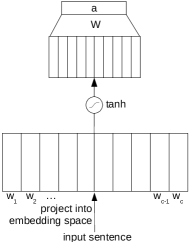
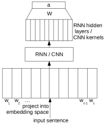
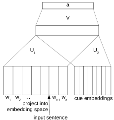
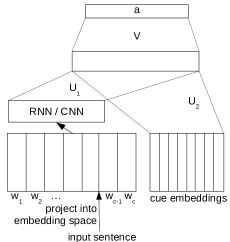
Figure 1: Internal attention on (1) input and (2) hidden representation. External attention on (3) input and (4) hidden representation. For the whole network structure, see Figure 3.

Weighted vs. Unweighted Selection. Pooling is unweighted selection: it outputs the selected values as is. In contrast, attention can be thought of as weighted selection: some input elements are highly weighted, others receive weights close to zero and are thereby effectively not selected. The advantage of weighted selection is that the model learns to decide based on the input how many values it should select. Pooling either selects all values (average pooling) or k values (k-max pooling). If there are more than k uncertainty cues in a sentence, pooling is not able to focus on all of them.

Sequence-agnostic vs. Sequence-preserving Selection. K-max pooling [Kalchbrenner et al. (2014] is sequence-preserving: it takes a long sequence as input and outputs a subsequence whose members are in the same order as in the original sequence. In contrast, attention is generally implemented as a weighted average of the input vectors. That means that all ordering information is lost and cannot be recovered by the next layer. As an alternative, we present and evaluate new sequence-preserving ways of attention. For uncertainty detection, this might help distinguishing phrases like “it is not uncertain that X is Basque” and “it is uncertain that X is not Basque”.

Internal vs. External Attention. Prior work calculates attention weights based on the input or hidden layers of the neural network. We call this internal attention. For uncertainty detection, it can be beneficial to give the model a lexicon of seed cue words or phrases. Thus, we provide the network with additional information to bear on identifying and summarizing features. This can simplify the training process by guiding the model to recognizing uncertainty cues. We call this external attention and show that it improves performance for uncertainty detection.

Previous work on attention and pooling has only considered a small number of the possible configurations along those dimensions of attention. However, the internal/external and un/weighted distinctions can potentially impact performance because external resources add information that can be critical for good performance and because weighting increases the flexibility and expressivity of neural network models. Also, word order is often critical for meaning and is therefore an important feature in NLP. Although our models are motivated by the characteristics of uncertainty detection, they could be useful for other NLP tasks as well.

Our main contributions are as follows. (i) We extend the design space of selection mechanisms for neural networks and conduct an extensive set of experiments testing various configurations along several dimensions of that space, including novel sequence-preserving and external attention mechanisms. (ii) To our knowledge, we are the first to apply convolutional and recurrent neural networks to uncertainty detection. We demonstrate the effectiveness of the proposed attention architectures for this task and set the new state of the art on a Wikipedia benchmark dataset. (iii) We publicly release our code for future research.

2 Models

Convolutional Neural Networks. CNNs have been successful for many NLP tasks since convolution and pooling can detect key features independent of their position in the sentence. Moreover, they can take advantage of word embeddings and their characteristics. Both properties are also essential for uncertainty detection since we need to detect cue phrases that can occur anywhere in the sentence; and since some notion of similarity improves performance if a cue phrase in the test data did not occur in the training data, but is similar to one that did. The CNN we use in this paper has one convolutional layer, 3-max pooling (see ?)), a fully connected hidden layer and a logistic output unit.

Recurrent Neural Networks. Different types of RNNs have been applied widely to NLP tasks, including language modeling [Bengio et al. (2000, Mikolov et al. (2010], machine translation [Cho et al. (2014, Bahdanau et al. (2015], relation classification [Zhang and Wang (2015] and entailment [Rocktäschel et al. (2016]. In this paper, we apply a bi-directional gated RNN (GRU) with gradient clipping and a logistic output unit. ?) showed that GRUs and LSTMs have similar performance, but GRUs are more efficient in training. The hidden layer $h$ of the GRU is parameterized by two matrices $W$ and $U$ and four additional matrices $W_{r}$, $U_{r}$ and $W_{z}$, $U_{z}$ for the reset gate $r$ and the update gate $z$ [Cho et al. (2014]:

$$r=\sigma(W_{r}x+U_{r}h^{t-1})$$ (1)

$$z=\sigma(W_{z}x+U_{z}h^{t-1})$$ (2)

$$h^{t}=z\odot h^{t-1}+(1-z)\odot\tilde{h}^{t}$$ (3)

$$\tilde{h}^{t}=\sigma(Wx+U(r\odot h^{t-1}))$$ (4)

$t$ is the index for the current time step, $\odot$ is element-wise multiplication and $\sigma$ is the sigmoid.

3 Attention

3.1 Architecture of the Attention Layer

We first define an attention layer $a$ for input $x$:

$$\alpha_{i} = \frac{\exp(f(x_{i}))}{\sum_{j}\exp(f(x_{j}))}$$ (5)

$$a_{i} = \alpha_{i}\cdot x_{i}$$ (6)

where $f$ is a scoring function, the $\alpha_{i}$ are the attention weights and each input $x_{i}$ is reweighted by its corresponding attention weight $\alpha_{i}$.

The most basic definition of $f$ is as a linear scoring function on the input $x$:

$$f(x_{i})=W^{T}x_{i}$$ (7)

$W$ are parameters that are learned in training.

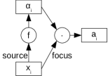
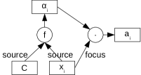
Figure 2: Schemes of focus and source: left: internal attention, right: external attention

3.2 Focus and Source of Attention

In this paper, we distinguish between focus and source of attention.

The focus of attention is the layer of the network that is reweighted by attention weights, corresponding to $x$ in Eq. 6. We consider two options for the application in uncertainty detection as shown in Figure 1: (i) the focus is on the input, i.e., the matrix of word vectors ((1) and (3)) and (ii) the focus is on the convolutional layer of the CNN or the hidden layers of the RNN ((2) and (4)). For focus on the input, we apply tanh to the word vectors (see part (1) of figure) to improve results.

The source of attention is the information source that is used to compute the attention weights, corresponding to the input of $f$ in Eq. 5.

Eq. 7 formalizes the case in which focus and source are identical (both are based only on $x$). We call this internal attention (see left part of Figure 2). An attention layer is called internal if both focus and source are based only on information internally available to the network (through input or hidden layers).

If we conceptualize attention in terms of source and focus, then a question that arises is whether we can make it more powerful by increasing the scope of the source beyond the input.

In this paper, we propose a way of expanding the source of attention by making an external resource $C$ available to the scoring function $f$:

$$f(x_{i})=f^{\prime}(x_{i},C)$$ (8)

We call this external attention (see right part of Figure 2). An attention layer is called external if its source includes an external resource.

The specific external-attention scoring function we use for uncertainty detection is parametrized by $U_{1}$, $U_{2}$ and $V$ and defined as follows:

$$f(x_{i})=\sum_{j}V^{T}\cdot\tanh(U_{1}\cdot x_{i}+U_{2}\cdot c_{j})$$ (9)

where $c_{j}$ is a vector representing a cue phrase $j$ of the training set. We compute $c_{j}$ as the average of the embeddings of the constituent words of $j$.

This attention layer scores an input word $x_{i}$ by comparing it with each cue vector $c_{j}$ and summing the results. The comparison is done using a fully connected hidden layer. Its weights $U_{1}$, $U_{2}$ and $V$ are learned during training. When using this scoring function in Eq. 5, each $\alpha_{i}$ is an assessment of how important $x_{i}$ is for uncertainty detection, taking into account our knowledge about cue phrases. Since we use embeddings to represent words and cues, uncertainty-indicating phrases that did not occur in training, but are similar to training cue phrases can also be recognized.

We use this novel attention mechanism for uncertainty detection, but it is also applicable to other tasks and domains as long as there is a set of vectors available that is analogous to our $c_{j}$ vectors, i.e., vectors that model relevance of embeddings to the task at hand (for an outlook, see Section 6).

3.3 Sequence-agnostic vs. Sequence-preserving Selection

So far, we have explained the basic architecture of an attention layer: computing attention weights and reweighting the input. We now turn to the integration of the attention layer into the overall network architecture, i.e., how it is connected to downstream components.

The most frequently used downstream connection of the attention layer is to take the average:

$$a=\sum_{i}a_{i}$$ (10)

We call this the average, not the sum, because the $\alpha_{i}$ are normalized to sum to 1 and the standard term for this is “weighted average”.

A variant is the k-max average:

$$a=\sum_{R(\alpha_{j})\leq k}a_{j}$$

where $R(\alpha_{j})$ is the rank of $\alpha_{j}$ in the list of activation weights $\alpha_{i}$ in descending order. This type of averaging is more similar to k-max pooling and may be more robust because elements with low weights (which may just be noise) will be ignored.

Averaging destroys order information that may be needed for NLP sequence classification tasks. Therefore, we also investigate a sequence-preserving method, k-max sequence:

$$a=[a_{j}|R(\alpha_{j})\leq k]$$ (11)

where $[a_{j}|P(a_{j})]$ denotes the subsequence of sequence $A=[a_{1},\ldots,a_{J}]$ from which members not satisfying predicate $P$ have been removed. Note that sequence $a$ is in the original order of the input, i.e., not sorted by value.

K-max sequence selects a subsequence of input vectors. Our last integration method is k-max pooling. It ranks each dimension of the vectors individually, thus the resulting values can stem from different input positions. This is the same as standard k-max pooling in CNNs except that each vector element in $a_{j}$ has been weighted (by its attention weight $\alpha_{j}$), whereas in standard k-max pooling it is considered as is. Below, we also refer to k-max sequence as “per-pos” and to k-max pooling as “per-dim” to clearly distinguish it from k-max pooling done by the CNN.

Combination with CNN and RNN Output.

Another question is whether we combine the attention result with the result of the convolutional or recurrent layer of the network. Since k-max pooling (CNN) and recurrent hidden layers with gates (RNN) have strengths complementary to attention, we experiment with concatenating the attention information to the neural sentence representations. The final hidden layer then has this form:

$$h=\mbox{tanh}(W_{1}a+W_{2}r+b)$$

with $r$ being either the CNN pooling result or the last hidden state of the RNN (see Figure 3).

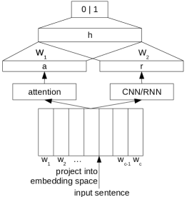
Figure 3: Network overview: combination of attention and CNN/RNN output. For details on attention, see Figure 1.

4 Experimental Setup and Results

4.1 Task and Setup

We evaluate on the two corpora of the CoNLL2010 hedge cue detection task [Farkas et al. (2010]: Wikipedia (11,111 sentences in train, 9634 in test) and Biomedical (14,541 train, 5003 test). It is a binary sentence classification task. For each sentence, the model has to decide whether it contains uncertain information.

For hyperparameter tuning, we split the training set into core-train (80%) and dev (20%) sets; see appendix for hyperparameter values. We use 400 dimensional word2vec [Mikolov et al. (2013] embeddings, pretrained on Wikipedia, with a special embedding for unknown words.

For evaluation, we apply the official shared task measure: $F_{1}$ of the uncertain class.

4.2 Baselines without Attention

Our baselines are a support vector machine (SVM) and two standard neural networks without attention, an RNN and a CNN. The SVM is a reimplementation of the top ranked system on Wikipedia in the CoNLL-2010 shared task [Georgescul (2010], with parameters set to ?)’s values; it uses bag-of-word (BOW) vectors that only include hedge cues. Our reimplementation is slightly better than the published result: 62.01 vs. 60.20 on wiki, 78.64 vs. 78.50 on bio.

	Model	wiki	bio
(1)	Baseline SVM	62.01$\star$	78.64$\star$
(2)	Baseline RNN	59.82$\star$	84.69
(3)	Baseline CNN	64.94	84.23

Table 1: $F_{1}$ results for UD. Baseline models without attention. $\star$ indicates significantly worse than best model (in bold).

	Model	wiki	bio
(2)	Baseline RNN	59.82$\star$	84.69
(4)	RNN attention-only	62.02$\star$	85.32
(5)	RNN combined	58.96$\star$	84.88
(3)	Baseline CNN	64.94$\star$	84.23
(6)	CNN attention-only	53.44$\star$	82.85
(7)	CNN combined	66.49	84.69

Table 2: $F_{1}$ results for UD. Attention-only vs. combined architectures. Sequence-agnostic weighted average for attention. $\star$ indicates significantly worse than best model (bold).

The results of the baselines are given in Table 1. The CNN (line 3) outperforms the SVM (line 1) on both datasets, presumably because it considers all words in the sentence – instead of only predefined hedge cues – and makes effective use of this additional information. The RNN (line 2) performs better than the SVM and CNN on biomedical data, but worse on Wikipedia. In Section 5.2, we investigate possible reasons for that.

4.3 Experiments with Attention Mechanisms

For the first experiments of this subsection, we use the sequence-agnostic weighted average for attention (see Eq. 10), the standard in prior work.

Attention-only vs. Combined Architecture. For the case of internal attention, we first remove the final pre-output layer of the standard RNN and the standard CNN to evaluate attention-only architectures. This architecture works well for RNNs but not for CNNs. The CNNs achieve better results when the pooling output (unweighted selection) is combined with the attention output (weighted selection). See Table 2 for $F_{1}$ scores.

The baseline RNN has the difficult task of remembering the entire sentence over long distances – the attention mechanism makes this task much easier. In contrast, the baseline CNN already has an effective mechanism for focusing on the key parts of the sentence: k-max pooling. Replacing k-max pooling with attention decreases the performance in this setup.

Since our main goal is to explore the benefits of adding attention to existing architectures (as opposed to developing attention-only architectures), we keep the standard pre-output layer of RNNs and CNNs in the remaining experiments and combine it with the attention layer as in Figure 3.

Focus and Source of Attention. We distinguish different focuses and sources of attention. For focus, we investigate two possibilities: the input to the network, i.e., word embeddings (F=W); or the hidden representations of the RNN or CNN (F=H). For source, we compare internal (S=I) and external attention (S=E). This gives rise to four configurations: (i) internal attention with focus on the first layer of the standard RNN/CNN (S=I, F=H), see lines (5) and (7) in Table 2, (ii) internal attention with focus on the input (S=I, F=W), (iii) external attention on the first layer of RNN/CNN (S=E, F=H) and (iv) external attention on the input (S=E, F=W). The results are provided in Table 3.

For both RNN (8) and CNN (13), the best result is obtained by focusing attention directly on the word embeddings. These results suggest that it is best to optimize the attention mechanism directly on the input, so that information can be extracted that is complementary to the information extracted by a standard RNN/CNN.

For focus on input (F=W), external attention (13) is significantly better than internal attention (11) for CNNs. Thus, by designing an architectural element – external attention – that makes it easier to identify hedge cue properties of words, the learning problem is apparently made easier.

For the RNN and F=W, external attention (10) is not better than internal attention (8): results are roughly tied for bio and wiki. Perhaps the combination of the external resource and the more indirect representation of the entire sentence produced by the RNN is difficult. In contrast, hedge cue patterns identified by convolutional filters of the CNN can be evaluated well based on external attention; e.g., if there is strong external-attention evidence for uncertainty, then the effect of a hedge cue pattern (hypothesized by a convolutional filter) on the final decision can be boosted.

In summary, the CNN with external attention achieves the best results overall. It is significantly better than the standard CNN that uses only pooling, both on Wikipedia and biomedical texts. This demonstrates that the CNN can make effective use of external information – a lexicon of uncertainty cues in our case.

	Model	S	F	wiki	bio
(2)	Baseline RNN	-	-	59.82$\star$	84.69
(5)	RNN combined	I	H	58.96$\star$	84.88
(8)	RNN combined	I	W	62.18$\star$	84.81
(9)	RNN combined	E	H	61.19$\star$	84.62
(10)	RNN combined	E	W	61.87$\star$	84.41
(3)	Baseline CNN	-	-	64.94$\star$	84.23$\star$
(7)	CNN combined	I	H	66.49	84.69
(11)	CNN combined	I	W	65.13$\star$	84.99
(12)	CNN combined	E	H	64.14$\star$	84.73
(13)	CNN combined	E	W	67.08	85.57

Table 3: $F_{1}$ results for UD. Focus (F) and source (S) of attention: Internal (I) vs external (E) attention; attention on word embeddings (W) vs. on hidden layers (H). Sequence-agnostic weighted average for attention. $\star$ indicates significantly worse than best model (bold).

Sequence-agnostic vs. Sequence-preserving. Commonly used attention mechanisms simply average the vectors in the focus of attention. This means that sequential information is not preserved. We use the term sequence-agnostic for this. In contrast, we propose to investigate sequence-preserving attention as presented in Section 3.3. We expect this to be important for many NLP tasks. Sequence-preserving attention is similar to k-max pooling which also selects an ordered subset of inputs. While traditional k-max pooling is unweighted, our sequence-preserving ways of attention still make use of the attention weights.

	average		k-max sequence
	all	k-max	per-dim	per-pos
Wiki	67.08	67.52	66.73	66.50
Bio	85.57	84.36	84.05	84.03

Table 4: $F_{1}$ results for UD. Model: CNN, S=E, F=W (13). Sequence-agnostic vs. sequence-preserving attention.

Table 4 compares k-max pooling, attention and two “hybrid” designs, as described in Section 3.3. We run these experiments only on the CNN with external attention focused on word embeddings (Table 3, line 13), the best performing configuration in the previous experiments.

First, we investigate what happens if we “discretize” attention and only consider the values with the top k attention weights. This increases performance on wiki (from 67.08 to 67.52) and decreases it on bio (from 85.57 to 84.36). We would not expect large differences since attention values tend to be peaked, so for common values of k ($k\geq 3$ in most prior work on k-max pooling) we are effectively comparing two similar weighted averages, one in which most summands get a weight of 0 (k-max average) and one in which most summands get weights close to 0 (average over all, i.e., standard attention).

Next, we compare sequence-agnostic with sequence-preserving attention. As described in Section 3.3, two variants are considered. In k-max pooling, we select the k largest weighted values per dimension (per-dim in Table 4). In contrast, k-max sequence (per-pos) selects all values of the k positions with the highest attention weights.

In Table 4, the sequence-preserving architectures are slightly worse than standard attention (i.e., sequence-agnostic averaging), but not significantly: performance is different by about half a point. This shows that k-max sequence and attention can similarly be used to select a subset of the information available, a parallel that has not been highlighted and investigated in detail before.

Although in this case, sequence-agnostic attention is better than sequence-preserving attention, we would not expect this to be true for all tasks. Our motivation for introducing sequence-preserving attention was that the semantic meaning of a sentence can vary depending on where an uncertainty cue occurs. However, the core of uncertainty detection is keyword and keyphrase detection; so, the overall sentence structure might be less important for this task. For tasks with a stronger natural language understanding component, such as summarization or relation extraction, on the other hand, we expect sequences of weighted vectors to outperform averaged vectors. In Section 6, we show that sequence-preserving attention indeed improves results on a sentiment analysis dataset.

4.4 Comparison to State of the Art

Table 5 compares our models with the state of the art on the uncertainty detection benchmark datasets. On Wikipedia, our CNN outperforms the state of the art by more than three points. On bio, the best model uses a large number of manually designed features and an exhaustive corpus preprocessing [Tang et al. (2010]. Our models achieve comparable results without preprocessing or feature engineering.

Model	wiki	bio
SVM [Georgescul (2010]	62.01	78.64
HMM [Li et al. (2014]	63.97	80.15
CRF + ling [Tang et al. (2010]	55.05	86.79
Our CNN with external attention	67.52	85.57

Table 5: Comparison of our best model with the state of the art

5 Analysis

5.1 Analysis of Attention

In an analysis of examples for which pooling alone (i.e., the standard CNN) fails, but attention correctly detects an uncertainty, two patterns emerge.

In the first pattern, we find that there are many cues that have more words than the filter size (which was 3 in our experiments), e.g., “it is widely expected”, “it has also been suggested”. The convolutional layer of the CNN is not able to detect phrases longer than the filter size while for attention there is no such restriction.

The second pattern consists of cues spread over the whole sentence, e.g., “Observations of the photosphere of 47 Ursae Majoris suggested that the periodicity could not be explained by stellar activity, making the planet interpretation more likely” where we have set the uncertainty cues that are distributed throughout the sentence in italics. Figure 4 shows the distribution of external attention weights computed by the CNN for this sentence. The CNN pays the most attention to the three words/phrases “suggested”, “not” and “more likely” that correspond almost perfectly to the true uncertainty cues. K-max pooling of standard CNNs, on the other hand, can only select the k maximum values per dimension, i.e., it can pick at most k uncertainty cues per dimension.

Figure 4: Attention weight heat map

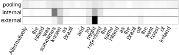
Figure 5: Pooling vs. internal vs. ext. attention

Pooling vs. Internal vs. External Attention.

Finally, we compare the information that pooling, internal and external attention extract. For pooling, we calculate the relative frequency that a value from an n-gram centered around a specific word is picked. For internal and external attention, we directly plot the attention weights $\alpha_{i}$. Figure 5 shows the results of the three mechanisms for an exemplary sentence. For a sample of randomly selected sentences, we observed similar patterns: Pooling forwards information from different parts all over the sentence. It has minor peaks at relevant n-grams (e.g. “was sometimes known as” or “so might represent”) but also at non-relevant parts (e.g. “Alternatively” or “the same island”). There is no clear focus on uncertainty cues. Internal attention is more focused on the relevant words. External attention finally has the clearest focus. (See appendix for more examples.)

5.2 Analysis of CNN vs RNN

While the results of the CNN and the RNN are comparable on bio, the CNN clearly outperforms the RNN on wiki. The datasets vary in several aspects, such as average sentence lengths (wiki: 21, bio: 27), size of vocabularies (wiki: 45.1k, bio: 25.3k), average number of out-of-vocabulary (OOV) words per sentence w.r.t. our word embeddings (wiki: 4.5, bio: 6.5), etc. All of those features can influence model performance, especially because of the different way of sentence processing: While the RNN merges all information into a single vector, the CNN extracts the most important phrases and ignores all the rest. In the following, we analyze the behavior of the two models w.r.t. sentence length and number of OOVs.

Figure 6 shows the $F_{1}$ scores on Wikipedia of the CNN and the RNN with external attention for different sentence lengths. The lengths have been accumulated, i.e., index 0 on the x-axis includes the scores for all sentences of length $l\in[0,10)$. Most sentences have lengths $l<50$. In this range, the CNN performs better than the RNN but the difference is small. For longer sentences, however, the CNN clearly outperforms the RNN. This could be one reason for the better overall performance.

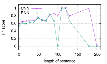
Figure 6: $F_{1}$ results for different sentence lengths

A similar plot for $F_{1}$ scores depending on the number of OOVs per sentence does not give additional insights into the model behaviors: The CNN performs better than the RNN independent of the number of OOVs (Figure in appendix).

Another important difference between CNN and RNN is the distribution of precision and recall. While on bio, precision and recall are almost equal for both models, the values vary on wiki:

	P	R
CNN	52.5	85.1
CNN + external attention	58.6	78.3
RNN	75.2	49.6
RNN + external attention	76.3	52.0

Those values suggest that the RNN predicts uncertainty more reluctantly than the CNN.

6 Outlook: Different Task

To investigate whether our attention methods are also applicable to other tasks, we evaluate them on the 2-class Stanford Sentiment Treebank (SST-2) dataset [Socher et al. (2013]. For a baseline model, we train a CNN similar to our uncertainty CNN but with convolutional filters of different widths, as proposed in [Kim (2014], and extend it with our attention layer. As cues for external attention, we use the most frequent positive phrases from the train set. Our model is much simpler than the state-of-the-art models for SST-2 but still achieves reasonable results.

Model	S	F	test set
Baseline CNN	-	-	84.84
CNN attention-only	I	H	83.56
CNN combined	I	H	85.22
CNN combined	I	W	86.11
CNN combined	E	H	86.06
CNN combined	E	W	86.89

Table 6: Accuracy on SST-2, different focus and source of attention.

average		k-max sequence
all	k-max	per-dim	per-pos
86.89	86.39	87.00	87.22

Table 7: Accuracy on SST-2, sequence-agnostic vs. sequence-preserving attention.

The results in Table 6 show the same trends as the CNN results in Table 3, suggesting that our methods are applicable to other tasks as well. Table 7 shows that the benefit of sequence-preserving attention is indeed task dependent. For sentiment analysis on SST-2, sequence-preserving methods outperform the sequence-agnostic ones.

7 Related Work

Uncertainty Detection. Uncertainty has been extensively studied in linguistics and NLP [Kiparsky and Kiparsky (1970, Karttunen (1973, Karttunen and Zaenen (2005], including modality [Saurí and Pustejovsky (2012, De Marneffe et al. (2012, Szarvas et al. (2012] and negation [Velldal et al. (2012, Baker et al. (2012]. ?), ?) and ?) conducted cross domain experiments. Domains studied include news [Saurí and Pustejovsky (2009], biomedicine [Vincze et al. (2008], Wikipedia [Ganter and Strube (2009] and social media [Wei et al. (2013]. Corpora such as FactBank [Saurí and Pustejovsky (2009] are annotated in detail with respect to perspective, level of factuality and polarity. ?) conducted uncertainty detection experiments on a version of FactBank extended by crowd sourcing. In this work, we use CoNLL 2010 shared task data [Farkas et al. (2010] since CoNLL provides larger train/test sets and the CoNLL annotation consists of only two labels (certain/uncertain) instead of various perspectives and degrees of uncertainty. When using uncertainty detection for information extraction tasks like KB population (Section 1), it is a reasonable first step to consider only two labels.

CNNs. Several studies showed that CNNs can handle diverse sentence classification tasks, including sentiment analysis [Kalchbrenner et al. (2014, Kim (2014], relation classification [Zeng et al. (2014, dos Santos et al. (2015] and paraphrase detection [Yin et al. (2016]. To our knowledge, we are the first to apply them to uncertainty detection.

RNNs. RNNs have mainly been used for sequence labeling or language modeling tasks with one output after each input token [Bengio et al. (2000, Mikolov et al. (2010]. Recently, it has been shown that they are also capable of encoding and restoring relevant information from a whole input sequence. This makes them applicable to machine translation [Cho et al. (2014, Bahdanau et al. (2015] and sentence classification tasks [Zhang and Wang (2015, Hermann et al. (2015, Rocktäschel et al. (2016]. In this study, we apply them to UD for the first time and compare their results with CNNs.

Attention has been mainly used for recurrent neural networks [Bahdanau et al. (2015, Rush et al. (2015, Hermann et al. (2015, Rocktäschel et al. (2016, Peng et al. (2015, Yang et al. (2016]. We integrate attention into CNNs and show that this is beneficial for uncertainty detection. Few studies in vision integrated attention into CNNs [Stollenga et al. (2014, Xiao et al. (2015, Chen et al. (2015] but this has not been used often in NLP so far. Exceptions are ?), ?) and ?). ?) used several layers of local and global attention in a complex machine translation model with a large number of parameters. Our reimplementation of their network performed poorly for uncertainty detection (51.51/66.57 on wiki/bio); we suspect that the reason is that ?)’s training set was an order of magnitude larger than ours. Our approach makes effective use of a much smaller training set. ?) compared attention based input representations and attention based pooling. Instead, our goal is to keep the convolutional and pooling layers unchanged and combine their strengths with attention. ?) applied a convolutional layer to compute attention weights. In this work, we concentrate on the commonly used feed forward layers for that. Comparing them to other options, such as convolution, is an interesting direction for future work.

Attention in the literature computes a weighted average with internal attention weights. In contrast, we investigate different strategies to incorporate attention information into a neural network. Also, we propose external attention. The underlying intuition is similar to attention for machine translation, which learns alignments between source and target sentences, or attention in question answering, which computes attention weights based on a question and a fact. However, these sources for attention are still internal information of the network (the input or previous output predictions). Instead, we learn weights based on an external source – a lexicon of cue phrases.

8 Conclusion

In this paper, we presented novel attention architectures for uncertainty detection: external attention and sequence-preserving attention. We conducted an extensive set of experiments with various configurations along different dimensions of attention, including different focuses and sources of attention and sequence-agnostic vs. sequence-preserving attention. For our experiments, we used two benchmark datasets for uncertainty detection and applied recurrent and convolutional neural networks to this task for the first time. Our CNNs with external attention improved state of the art by more than 3.5 $F_{1}$ points on a Wikipedia benchmark. Finally, we showed in an outlook that our architectures are applicable to sentiment classification as well. Investigations of other sequence classification tasks are future work. We made our code publicly available for future research (http://cistern.cis.lmu.de).

Appendix A Supplementary Material

A.1 Parameter Tuning

All parameters and learning rate schedule decisions are based on results on the development set (20% of the official training set). After tuning the hyperparameters (see Tables 8 and 9), the networks are re-trained on the whole training set.

We trained the CNNs with stochastic gradient descent and a fixed learning rate of 0.03. For the RNNs, we used Adagrad [Duchi et al. (2011] with an initial learning rate of 0.1. For all models, we used mini-batches of size 10 and applied L2 regularization with a weight of 1e-5. To determine the number of training epochs, we looked for epochs with peak performances on the development set.

	Model	# conv	filter	# hidden	# att
		filters	width	units	hidden
					units
CNN wiki	(3)	200	3	200	-
	(6)	100	3	500	-
	(7)	200	3	200	-
	(11)	200	3	200	-
	(12)	200	3	200	200
	(13)	100	3	200	200
CNN bio	(3)	200	3	500	-
	(6)	100	3	200	-
	(7)	100	3	500	-
	(11)	200	3	200	-
	(12)	200	3	500	100
	(13)	200	3	50	100

Table 8: Result of parameter tuning for CNN (“att hidden units” is the number of units in the hidden layer of the attention component); Model numbers refer to numbers in the main paper

	Model	# rnn	# hidden	# att
		hidden	units	hidden
		units		units
RNN wiki	(2)	10	100	-
	(4)	10	100	-
	(5)	10	200	-
	(8)	10	100	-
	(9)	30	200	200
	(10)	10	200	100
RNN bio	(2)	10	500	-
	(4)	10	500	-
	(5)	10	50	-
	(8)	10	50	-
	(9)	30	100	200
	(10)	10	50	200

Table 9: Result of parameter tuning for RNN

A.2 Additional Examples: Attention Weights

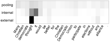
Figure 7: Pooling vs. internal attention vs. external attention

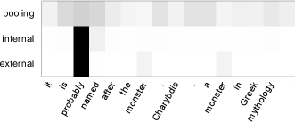
Figure 8: Pooling vs. internal attention vs. external attention

Figure 7 and Figure 8 compare pooling, internal attention and external attention for randomly picked examples from the test set. Again, pooling extracts values from all over the sentence while internal and external attention learn to focus on words which can indicate uncertainty (e.g. “thought” or “probably”).

A.3 Additional Figure for Analysis: Results Depending on Number of OOVs

Figure 9 plots the $F_{1}$ scores of the CNN and RNN with external attention w.r.t. the number of out-of-vocabulary (OOV) words in the sentences. The number of OOVs have been accumulated, i.e., index 0 on the x-axis includes the score for all sentences with a number of OOVs in [0,10), etc.

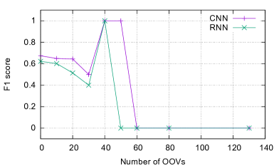
Figure 9: $F_{1}$ results for different numbers of OOVs in sentence

References

- [Allamanis et al. (2016] Miltiadis Allamanis, Hao Peng, and Charles Sutton. 2016. A convolutional attention network for extreme summarization of source code. In Proceedings of The 33rd International Conference on Machine Learning (ICML-16), ICML ’16, pages 2091–2100, New York City, NY, USA, June. ACM.
- [Bahdanau et al. (2015] Dzmitry Bahdanau, Kyunghyun Cho, and Yoshua Bengio. 2015. Neural machine translation by jointly learning to align and translate. In 3rd International Conference on Learning Representations (ICLR), San Diego, California, USA, May.
- [Baker et al. (2012] Kathryn Baker, Michael Bloodgood, Bonnie J Dorr, Chris Callison-Burch, Nathaniel W Filardo, Christine Piatko, Lori Levin, and Scott Miller. 2012. Use of modality and negation in semantically-informed syntactic MT. Computational Linguistics, 38:411–438.
- [Bengio et al. (2000] Yoshua Bengio, Réjean Ducharme, Pascal Vincent, and Christian Janvin. 2000. A neural probabilistic language model. Journal of Machine Learning Research, 3:1137–1155.
- [Chen et al. (2015] Kan Chen, Jiang Wang, Liang-Chieh Chen, Haoyuan Gao, Wei Xu, and Ram Nevatia. 2015. Abc-cnn: An attention based convolutional neural network for visual question answering. Technical Report. arXiv:1511.05960.
- [Cho et al. (2014] Kyunghyun Cho, Bart van Merrienboer, Caglar Gulcehre, Dzmitry Bahdanau, Fethi Bougares, Holger Schwenk, and Yoshua Bengio. 2014. Learning phrase representations using rnn encoder–decoder for statistical machine translation. In Proceedings of the 2014 Conference on Empirical Methods in Natural Language Processing (EMNLP), pages 1724–1734, Doha, Qatar, October. Association for Computational Linguistics.
- [Chung et al. (2014] Junyoung Chung, Caglar Gulcehre, KyungHyun Cho, and Yoshua Bengio. 2014. Empirical evaluation of gated recurrent neural networks on sequence modeling. arXiv preprint arXiv:1412.3555.
- [Collobert et al. (2011] Ronan Collobert, Jason Weston, Léon Bottou, Michael Karlen, Koray Kavukcuoglu, and Pavel Kuksa. 2011. Natural language processing (almost) from scratch. Journal of Machine Learning Research, 12:2493–2537.
- [De Marneffe et al. (2012] Marie-Catherine De Marneffe, Christopher D Manning, and Christopher Potts. 2012. Did it happen? the pragmatic complexity of veridicality assessment. Computational linguistics, 38:335–367.
- [Díaz et al. (2016] Noa P. Cruz Díaz, Maite Taboada, and Ruslan Mitkov. 2016. A machine-learning approach to negation and speculation detection for sentiment analysis. Journal of the Association for Information Science and Technology (JASIST), 67(9):2118–2136.
- [dos Santos et al. (2015] Cicero dos Santos, Bing Xiang, and Bowen Zhou. 2015. Classifying relations by ranking with convolutional neural networks. In Proceedings of the 53rd Annual Meeting of the Association for Computational Linguistics and the 7th International Joint Conference on Natural Language Processing (Volume 1: Long Papers), pages 626–634, Beijing, China, July. Association for Computational Linguistics.
- [Duchi et al. (2011] John Duchi, Elad Hazan, and Yoram Singer. 2011. Adaptive subgradient methods for online learning and stochastic optimization. Journal of Machine Learning Research, 12:2121–2159.
- [Farkas et al. (2010] Richárd Farkas, Veronika Vincze, György Móra, János Csirik, and György Szarvas. 2010. The conll-2010 shared task: Learning to detect hedges and their scope in natural language text. In Proceedings of the Fourteenth Conference on Computational Natural Language Learning, pages 1–12, Uppsala, Sweden, July. Association for Computational Linguistics.
- [Ganter and Strube (2009] Viola Ganter and Michael Strube. 2009. Finding hedges by chasing weasels: Hedge detection using wikipedia tags and shallow linguistic features. In Proceedings of the ACL-IJCNLP 2009 Conference Short Papers, pages 173–176, Suntec, Singapore, August. Association for Computational Linguistics.
- [Georgescul (2010] Maria Georgescul. 2010. A hedgehop over a max-margin framework using hedge cues. In Proceedings of the Fourteenth Conference on Computational Natural Language Learning, pages 26–31, Uppsala, Sweden, July. Association for Computational Linguistics.
- [He and Golub (2016] Xiaodong He and David Golub. 2016. Character-level question answering with attention. In Proceedings of the 2016 Conference on Empirical Methods in Natural Language Processing, pages 1598–1607, Austin, Texas, November. Association for Computational Linguistics.
- [Hermann et al. (2015] Karl Moritz Hermann, Tomáš Kočiský, Edward Grefenstette, Lasse Espeholt, Will Kay, Mustafa Suleyman, and Phil Blunsom. 2015. Teaching machines to read and comprehend. In NIPS’15 Proceedings of the 28th International Conference on Neural Information Processing Systems, pages 1693–1701, Montreal, Canada. MIT Press.
- [Kalchbrenner et al. (2014] Nal Kalchbrenner, Edward Grefenstette, and Phil Blunsom. 2014. A convolutional neural network for modelling sentences. In Proceedings of the 52nd Annual Meeting of the Association for Computational Linguistics (Volume 1: Long Papers), pages 655–665, Baltimore, Maryland, June. Association for Computational Linguistics.
- [Karttunen and Zaenen (2005] Lauri Karttunen and Annie Zaenen. 2005. Veridicity. In Graham Katz, James Pustejovsky, and Frank Schilder, editors, Annotating, Extracting and Reasoning about Time and Events, number 05151 in Dagstuhl Seminar Proceedings, Dagstuhl, Germany. Internationales Begegnungs- und Forschungszentrum für Informatik (IBFI), Schloss Dagstuhl, Germany.
- [Karttunen (1973] Lauri Karttunen. 1973. Presuppositions of compound sentences. Linguistic Inquiry, 4:169–196.
- [Kim (2014] Yoon Kim. 2014. Convolutional neural networks for sentence classification. In Proceedings of the 2014 Conference on Empirical Methods in Natural Language Processing (EMNLP), pages 1746–1751, Doha, Qatar, October. Association for Computational Linguistics.
- [Kiparsky and Kiparsky (1970] Paul Kiparsky and Carol Kiparsky. 1970. Fact. Progress in Linguistics, pages 143–173.
- [Li et al. (2014] Xiujun Li, Wei Gao, and Jude W Shavlik. 2014. Detecting semantic uncertainty by learning hedge cues in sentences using an hmm. In SIGIR 2014 Workshop on Semantic Matching in Information Retrieval, Queensland, Australia, July.
- [Manning et al. (2014] Christopher Manning, Mihai Surdeanu, John Bauer, Jenny Finkel, Steven Bethard, and David McClosky. 2014. The stanford corenlp natural language processing toolkit. In Proceedings of 52nd Annual Meeting of the Association for Computational Linguistics: System Demonstrations, pages 55–60, Baltimore, Maryland, June. Association for Computational Linguistics.
- [Meng et al. (2015] Fandong Meng, Zhengdong Lu, Mingxuan Wang, Hang Li, Wenbin Jiang, and Qun Liu. 2015. Encoding source language with convolutional neural network for machine translation. In Proceedings of the 53rd Annual Meeting of the Association for Computational Linguistics and the 7th International Joint Conference on Natural Language Processing (Volume 1: Long Papers), pages 20–30, Beijing, China, July. Association for Computational Linguistics.
- [Mikolov et al. (2010] Tomas Mikolov, Martin Karafiát, Lukás Burget, Jan Cernocký, and Sanjeev Khudanpur. 2010. Recurrent neural network based language model. In INTERSPEECH 2010, 11th Annual Conference of the International Speech Communication Association, pages 1045–1048, Makuhari, Chiba, Japan, September.
- [Mikolov et al. (2013] Tomas Mikolov, Kai Chen, Greg Corrado, and Jeffrey Dean. 2013. Efficient estimation of word representations in vector space. In Proceedings of Workshop at 1st International Conference on Learning Representations (ICLR), Scottsdale, Arizona, USA, May.
- [Peng et al. (2015] Baolin Peng, Zhengdong Lu, Hang Li, and Kam-Fai Wong. 2015. Towards neural network-based reasoning. In arXiv preprint arXiv:1508.05508.
- [Rocktäschel et al. (2016] Tim Rocktäschel, Edward Grefenstette, Karl Moritz Hermann, Tomáš Kočiskỳ, and Phil Blunsom. 2016. Reasoning about entailment with neural attention. In 4th International Conference on Learning Representations (ICLR), San Juan, Puerto Rico, May.
- [Rush et al. (2015] Alexander M. Rush, Sumit Chopra, and Jason Weston. 2015. A neural attention model for abstractive sentence summarization. In Proceedings of the 2015 Conference on Empirical Methods in Natural Language Processing, pages 379–389, Lisbon, Portugal, September. Association for Computational Linguistics.
- [Saurí and Pustejovsky (2009] Roser Saurí and James Pustejovsky. 2009. Factbank: A corpus annotated with event factuality. Language Resources and Evaluation, 43:227–268.
- [Saurí and Pustejovsky (2012] Roser Saurí and James Pustejovsky. 2012. Are you sure that this happened? Assessing the factuality degree of events in text. Computational Linguistics, 38:261–299.
- [Socher et al. (2013] Richard Socher, Alex Perelygin, Jean Wu, Jason Chuang, Christopher D. Manning, Andrew Ng, and Christopher Potts. 2013. Recursive deep models for semantic compositionality over a sentiment treebank. In Proceedings of the 2013 Conference on Empirical Methods in Natural Language Processing, pages 1631–1642, Seattle, Washington, USA, October. Association for Computational Linguistics.
- [Stollenga et al. (2014] Marijn F Stollenga, Jonathan Masci, Faustino Gomez, and Jürgen Schmidhuber. 2014. Deep networks with internal selective attention through feedback connections. In NIPS’14 Proceedings of the 27th International Conference on Neural Information Processing Systems, pages 3545–3553, Montreal, Canada, December.
- [Szarvas et al. (2012] György Szarvas, Veronika Vincze, Richárd Farkas, György Móra, and Iryna Gurevych. 2012. Cross-genre and cross-domain detection of semantic uncertainty. Computational Linguistics, 38:335–367.
- [Tang et al. (2010] Buzhou Tang, Xiaolong Wang, Xuan Wang, Bo Yuan, and Shixi Fan. 2010. A cascade method for detecting hedges and their scope in natural language text. In Proceedings of the Fourteenth Conference on Computational Natural Language Learning, pages 13–17, Uppsala, Sweden, July. Association for Computational Linguistics.
- [Velldal et al. (2012] Erik Velldal, Lilja Øvrelid, Jonathon Read, and Stephan Oepen. 2012. Speculation and negation: Rules, rankers, and the role of syntax. Computational linguistics, 38:369–410.
- [Vincze et al. (2008] Veronika Vincze, György Szarvas, Richárd Farkas, György Móra, and János Csirik. 2008. The bioscope corpus: biomedical texts annotated for uncertainty, negation and their scopes. BMC bioinformatics, 9:1–9.
- [Vincze (2014a] Veronika Vincze. 2014a. Uncertainty detection in hungarian texts. In Proceedings of COLING 2014, the 25th International Conference on Computational Linguistics: Technical Papers, pages 1844–1853, Dublin, Ireland, August. Dublin City University and Association for Computational Linguistics.
- [Vincze (2014b] Veronika Vincze. 2014b. Uncertainty Detection in Natural Language Texts. Ph.D. thesis, University of Szeged.
- [Wang et al. (2016] Linlin Wang, Zhu Cao, Gerard de Melo, and Zhiyuan Liu. 2016. Relation classification via multi-level attention cnns. In Proceedings of the 54th Annual Meeting of the Association for Computational Linguistics (Volume 1: Long Papers), pages 1298–1307, Berlin, Germany, August. Association for Computational Linguistics.
- [Wei et al. (2013] Zhongyu Wei, Junwen Chen, Wei Gao, Binyang Li, Lanjun Zhou, Yulan He, and Kam-Fai Wong. 2013. An empirical study on uncertainty identification in social media context. In Proceedings of the 51st Annual Meeting of the Association for Computational Linguistics (Volume 2: Short Papers), pages 58–62, Sofia, Bulgaria, August. Association for Computational Linguistics.
- [Xiao et al. (2015] Tianjun Xiao, Yichong Xu, Kuiyuan Yang, Jiaxing Zhang, Yuxin Peng, and Zheng Zhang. 2015. The application of two-level attention models in deep convolutional neural network for fine-grained image classification. In IEEE Conference on Computer Vision and Pattern Recognition, CVPR, pages 842–850, Boston, MA, USA, June.
- [Yang et al. (2016] Zichao Yang, Diyi Yang, Chris Dyer, Xiaodong He, Alex Smola, and Eduard Hovy. 2016. Hierarchical attention networks for document classification. In Proceedings of the 2016 Conference of the North American Chapter of the Association for Computational Linguistics: Human Language Technologies, pages 1480–1489, San Diego, California, June. Association for Computational Linguistics.
- [Yin and Schütze (2015] Wenpeng Yin and Hinrich Schütze. 2015. Multichannel variable-size convolution for sentence classification. In Proceedings of the Nineteenth Conference on Computational Natural Language Learning, pages 204–214, Beijing, China, July. Association for Computational Linguistics.
- [Yin et al. (2016] Wenpeng Yin, Hinrich Schütze, Bing Xiang, and Bowen Zhou. 2016. Abcnn: Attention-based convolutional neural network for modeling sentence pairs. Transactions of the Association for Computational Linguistics, 4:259–272.
- [Zeng et al. (2014] Daojian Zeng, Kang Liu, Siwei Lai, Guangyou Zhou, and Jun Zhao. 2014. Relation classification via convolutional deep neural network. In Proceedings of COLING 2014, the 25th International Conference on Computational Linguistics: Technical Papers, pages 2335–2344, Dublin, Ireland, August. Dublin City University and Association for Computational Linguistics.
- [Zhang and Wang (2015] Dongxu Zhang and Dong Wang. 2015. Relation classification via recurrent neural network. Technical Report. arXiv:1508.01006.
- [Zhou et al. (2015] Huiwei Zhou, Huan Yang, Long Chen, Zhenwei Liu, Jianjun Ma, and Degen Huang. 2015. Combining feature-based and instance-based transfer learning approaches for cross-domain hedge detection with multiple sources. In Social Media Processing, volume 568, pages 225–232. Springer.
- [Zhou et al. (2016] Peng Zhou, Zhenyu Qi, Suncong Zheng, Jiaming Xu, Hongyun Bao, and Bo Xu. 2016. Text classification improved by integrating bidirectional lstm with two-dimensional max pooling. In Proceedings of COLING 2016, the 26th International Conference on Computational Linguistics: Technical Papers, pages 3485–3495, Osaka, Japan, December. The COLING 2016 Organizing Committee.