The NuSTAR Serendipitous Survey: the 40 Month Catalog and the Properties of the Distant High Energy X-ray Source Population

Abstract

We present the first full catalog and science results for the NuSTAR serendipitous survey. The catalog incorporates data taken during the first 40 months of NuSTAR operation, which provide $\approx 20$ Ms of effective exposure time over $331$ fields, with an areal coverage of $13$ deg², and $497$ sources detected in total over the $3$–$24$ keV energy range. There are $276$ sources with spectroscopic redshifts and classifications, largely resulting from our extensive campaign of ground-based spectroscopic followup. We characterize the overall sample in terms of the X-ray, optical, and infrared source properties. The sample is primarily comprised of active galactic nuclei (AGNs), detected over a large range in redshift from $z=0.002$ to $3.4$ (median of $\left<z\right>=0.56$), but also includes $16$ spectroscopically confirmed Galactic sources. There is a large range in X-ray flux, from $\log(f_{\rm 3-24keV}/\mathrm{erg\ s^{-1}\ cm^{-2}})\approx-14$ to $-11$, and in rest-frame $10$–$40$ keV luminosity, from $\log(L_{\rm 10-40keV}/\mathrm{erg\ s^{-1}})\approx 39$ to $46$, with a median of $44.1$. Approximately $79\%$ of the NuSTAR sources have lower energy ($<10$ keV) X-ray counterparts from XMM-Newton, Chandra, and Swift XRT. The mid-infrared (MIR) analysis, using WISE all-sky survey data, shows that MIR AGN color selections miss a large fraction of the NuSTAR-selected AGN population, from $\approx 15\%$ at the highest luminosities ($L_{\rm X}>10^{44}$ erg s^-1) to $\approx 80\%$ at the lowest luminosities ($L_{\rm X}<10^{43}$ erg s^-1). Our optical spectroscopic analysis finds that the observed fraction of optically obscured AGNs (i.e., the Type 2 fraction) is $F_{\rm Type\ 2}=53^{+14}_{-15}\%$, for a well-defined subset of the $8$–$24$ keV selected sample. This is higher, albeit at a low significance level, than the Type 2 fraction measured for redshift- and luminosity-matched AGNs selected by $<10$ keV X-ray missions.

1. Introduction

Since the late 1970s, which saw the advent of focusing X-ray observatories in space (e.g., Giacconi et al. 1979), X-ray surveys have provided fundamental advances in our understanding of growing supermassive black holes (e.g., Fabian & Barcons 1992; Brandt & Hasinger 2005; Alexander & Hickox 2012; Brandt & Alexander 2015). X-rays provide the most direct and efficient means of identifying active galactic nuclei (AGNs; the sites of rapid mass accretion onto supermassive black holes), since the effects of both line-of-sight absorption and dilution by host-galaxy light are comparatively low at X-ray energies. The collection of X-ray surveys over the last few decades have ranged from wide-area all-sky surveys to deep pencil-beam surveys, allowing the evolution of AGN obscuration and the X-ray luminosity function to be measured for a wide range in luminosity and redshift (up to $z\approx 5$; e.g., see Brandt & Alexander 2015 for a review). The deepest surveys with Chandra and XMM-Newton have directly resolved the majority ($\approx 70$–$90\%$) of the $\lesssim 8$ keV cosmic X-ray background (CXB) into individual objects (e.g., Worsley et al. 2005; Hickox & Markevitch 2006; Xue et al. 2012).

Until very recently, the most sensitive X-ray surveys (e.g., with Chandra and XMM-Newton) have been limited to photon energies of $<10$ keV, and are therefore biased against the identification of heavily obscured AGNs (for which the line-of-sight column density exceeds $N_{\rm H}\sim\mathrm{a\ few}\times 10^{23}$ cm^-2). This bias is especially strong at $z\lesssim 1$, but becomes less so for higher redshifts where the spectral features of absorption, and the penetrating higher energy X-rays, are shifted into the observed-frame X-ray energy window. The result is a complicated AGN selection function, which is challenging to correct for without a full knowledge of the prevalence of highly absorbed systems. These photon energies are also low compared to the peak of the CXB (at $\approx 20$–$30$ keV), meaning that spectral extrapolations are required to characterize the AGN population responsible for the CXB peak. High energy ($>10$ keV) X-ray surveys with non-focusing X-ray observatories (e.g., Swift BAT and INTEGRAL) have directly resolved $\approx 1$–$2\%$ of the CXB peak into individual AGNs (Krivonos et al., 2007; Ajello et al., 2008; Bottacini et al., 2012). These surveys have been successful in characterizing the local high-energy emitting AGN population (e.g., Tueller et al., 2008; Burlon et al., 2011; Vasudevan et al., 2013; Ricci et al., 2015) but, being largely confined to $z\lesssim 0.1$, there is limited scope for evolutionary studies.

A great breakthrough in studying the high-energy X-ray emitting population is the Nuclear Spectroscopic Telescope Array (NuSTAR; Harrison et al. 2013), the first orbiting observatory with the ability to focus X-ray light at energies $>10$ keV, resulting in a two orders of magnitude increase in sensitivity over previous non-focusing missions. This has opened up the possibility to study large, cleanly selected samples of high-energy emitting AGNs in the distant universe for the first time. The NuSTAR extragalactic survey program has provided the first measurements of the $>10$ keV AGN luminosity functions at $z>0.1$ (Aird et al., 2015b), and has directly resolved a large fraction ($35\pm 5\%$) of the CXB at $8$–$24$ keV (Harrison et al., 2016). In addition, both the survey program and targetted NuSTAR campaigns have demonstrated the importance of high-energy coverage for accurately constraining the intrinsic properties of distant AGNs (e.g., Del Moro et al., 2014; Lansbury et al., 2014; Luo et al., 2014; Civano et al., 2015; Lansbury et al., 2015; LaMassa et al., 2016), especially in the case of the most highly absorbed Compton-thick (CT) systems (where $N_{\rm H}>1.5\times 10^{24}$ cm^-2).

The NuSTAR extragalactic survey is the largest scientific program, in terms of time investment, undertaken with NuSTAR and is one of the highest priorities of the mission. There are two main “blind survey” components. Firstly, deep blank-field NuSTAR surveys have been performed in the following well-studied fields: the Extended Chandra Deep Field South (ECDFS; Lehmer et al. 2005), for which the total areal coverage with NuSTAR is $\approx 0.33$ $\mathrm{deg}^{2}$ (Mullaney et al. 2015, hereafter M15); the Cosmic Evolution Survey field (COSMOS; Scoville et al. 2007), which has $\approx 1.7$ $\mathrm{deg}^{2}$ of NuSTAR coverage (Civano et al. 2015, hereafter C15); the Extended Groth Strip (EGS; Groth et al. 1994), with $\approx 0.25$ $\mathrm{deg}^{2}$ of coverage (Aird et al., in prep.); the northern component of the Great Observatories Origins Deep Survey North (GOODS-N; Dickinson et al. 2003), with $\approx 0.07$ $\mathrm{deg}^{2}$ of coverage (Del Moro et al., in prep.); and the Ultra Deep Survey field (UDS; Lawrence et al. 2007), with $\approx 0.4$ $\mathrm{deg}^{2}$ of coverage (Masini et al., in prep.). Secondly, a wide-area “serendipitous survey” has been performed by searching the majority of NuSTAR pointings for chance background sources. An initial look at $10$ serendipitous survey sources was presented in Alexander et al. (2013). Serendipitous surveys represent an efficient and economical way to sample wide sky areas, and provide substantial data sets with which to examine the X-ray emitting population and search for extreme sources. They have been undertaken with many X-ray missions over the last few decades (e.g., Gioia et al. 1990; Comastri et al. 2001; Fiore et al. 2001; Harrison et al. 2003; Nandra et al. 2003; Gandhi et al. 2004; Kim et al. 2004; Ueda et al. 2005; Watson et al. 2009; Evans et al. 2010, 2014).

In this paper, we describe the NuSTAR serendipitous survey and present the first catalog, compiled from data which span the first $40$ months of NuSTAR operation. The serendipitous survey is a powerful component of the NuSTAR survey programme, with the largest overall sample size, the largest areal coverage ($\approx 13$ $\mathrm{deg}^{2}$), and regions with comparable sensitivity to the other NuSTAR surveys in well-studied fields. Section 2 details the NuSTAR observations, data reduction, source detection, and photometry. We match to counterparts at lower X-ray energies (from Chandra, XMM-Newton, and Swift XRT; Section 3.1), and at optical and infrared (IR) wavelengths (Section 3.2). We have undertaken an extensive campaign of ground-based spectroscopic followup, crucial for obtaining source redshifts and classifications, which is described in Section 3.3. Our results for the X-ray, optical, and IR properties of the overall sample are presented in Sections 4.1, 4.2, and 4.3, respectively. We summarize the main results in Section 5. All uncertainties and limits are quoted at the $90\%$ confidence level, unless otherwise stated. We assume the flat $\Lambda$CDM cosmology from WMAP7 (Komatsu et al., 2011).

2. The NuSTAR Data

The NuSTAR observatory (launched in 2012 June; Harrison et al. 2013) is comprised of two independent telescopes (A and B), identical in design, the focal plane modules of which are hereafter referred to as FPMA and FPMB. The modules have fields-of-view (FoVs) of $\approx 12\arcmin\times 12\arcmin$, which overlap in sky coverage. The observatory is sensitive between $3$ keV and $78$ keV. The main energy band that we focus on here is the $3$–$24$ keV band; this is the most useful band for the relatively faint sources detected in the NuSTAR extragalactic surveys, since the combination of instrumental background and a decrease in effective area with increasing energy means that source photons are unlikely to be detected at higher energies (except for the brightest sources). NuSTAR provides over an order of magnitude improvement in angular resolution compared to previous generation hard X-ray observatories: the point-spread function (PSF) has a full width at half maximum (FWHM) of $18\arcsec$ and a half-power diameter of $58\arcsec$, and is relatively constant across the FoV. The astrometric accuracy of NuSTAR is $8\arcsec$ for the brightest targets ($90\%$ confidence; Harrison et al. 2013). This worsens with decreasing photon counts, reaching a positional accuracy of $\approx 20\arcsec$ for the faintest sources (as we demonstrate in Section 3.1).

Here we describe the observations, data reduction and data-analysis procedures used for the NuSTAR serendipitous survey: Section 2.1 describes the NuSTAR observations which have been incorporated as part of the survey; Section 2.2 details the data reduction procedures used to generate the NuSTAR science data; Section 2.3 provides details of the source detection approach; Section 2.4 outlines the photometric measurements for source counts, band ratios, fluxes and luminosities; and Section 2.5 describes the final source catalog.

2.1. The serendipitous survey observations

The serendipitous survey is the largest area blind survey undertaken with NuSTAR. The survey is achieved by searching the background regions of almost every non-survey NuSTAR pointing for background sources unassociated with the original science target. The survey approach is well-suited to NuSTAR since there are generally large regions of uncontaminated background. We exclude from the survey NuSTAR fields with bright science targets, identified as fields with $>10^{6}$ counts within $120^{\prime\prime}$ of the on-axis position. We also exclude the dedicated extragalactic (COSMOS, ECDFS, EGS, GOODS-N, UDS) and Galactic survey fields (the Galactic center survey; Mori et al. 2015; Hong et al. 2016; and the Norma Arm survey; Fornasini et al., in prep.).

Over the period from 2012 July to 2015 November, which is the focus of the current study, there are $510$ individual NuSTAR exposures which have been incorporated into the serendipitous survey. These exposures were performed over $331$ unique fields (i.e., $331$ individual sky regions, each with contiguous coverage comprised of one or more NuSTAR exposures), yielding a total sky area coverage of $13$ deg². Table 1 lists the fields chronologically, and provides the following details for each field: the name of the primary NuSTAR science target; the number of NuSTAR exposures; the individual NuSTAR observation ID(s); the observation date(s); the pointing coordinates; the exposure time(s); the number of serendipitous sources detected; and flags to indicate the NuSTAR fields which were used in the Aird et al. (2015b) and Harrison et al. (2016) studies.

Table 1Details of the individual NuSTAR observations which make up the serendipitous survey

Field ID	Science Target	$N_{\rm obs}$	Obs. ID	Obs. Date	R.A. (∘)	Decl. (∘)	$t_{\rm exp}$ (ks)	$N_{\rm serendips}$	A15	H16
(1)	(2)	(3)	(4)	(5)	(6)	(7)	(8)	(9)	(10)	(11)
1	2MASX J05081967+1721483	1	60006011002	2012-07-23	77.08	17.36	16.6	0	0	0
2	Bkgd BII -11.2	1	10060003001	2012-07-24	71.11	28.38	8.9	0	0	0
3	2MASX J04234080+0408017	2	$\cdots$	$\cdots$	$\cdots$	$\cdots$	12.3	2	1	1
3a		$\cdots$	60006005002	2012-07-25	65.92	4.13	6.4	$\cdots$	$\cdots$	$\cdots$
3b		$\cdots$	60006005003	2012-07-25	65.92	4.13	5.9	$\cdots$	$\cdots$	$\cdots$
4	IC 4329A	1	60001045002	2012-08-12	207.33	-30.31	177.3	2	0	1
5	Mrk 231	2	$\cdots$	$\cdots$	$\cdots$	$\cdots$	74.9	4	1	1
5a		$\cdots$	60002025002	2012-08-26	194.06	56.87	44.3	$\cdots$	$\cdots$	$\cdots$
5b		$\cdots$	60002025004	2013-05-09	194.06	56.87	30.6	$\cdots$	$\cdots$	$\cdots$
6	NGC 7582	2	$\cdots$	$\cdots$	$\cdots$	$\cdots$	33.4	2	0	1
6a		$\cdots$	60061318002	2012-08-31	349.60	-42.37	17.7	$\cdots$	$\cdots$	$\cdots$
6b		$\cdots$	60061318004	2012-09-14	349.60	-42.37	15.7	$\cdots$	$\cdots$	$\cdots$
7	AE Aqr	4	$\cdots$	$\cdots$	$\cdots$	$\cdots$	134.2	2	1	1
7a		$\cdots$	30001120002	2012-09-04	310.04	-0.87	7.2	$\cdots$	$\cdots$	$\cdots$
7b		$\cdots$	30001120003	2012-09-05	310.04	-0.87	40.5	$\cdots$	$\cdots$	$\cdots$
7c		$\cdots$	30001120004	2012-09-05	310.04	-0.87	76.6	$\cdots$	$\cdots$	$\cdots$
7d		$\cdots$	30001120005	2012-09-07	310.04	-0.87	9.8	$\cdots$	$\cdots$	$\cdots$
8	NGC 612	1	60061014002	2012-09-14	23.49	-36.49	17.9	0	0	1
9	3C 382	1	60061286002	2012-09-18	278.76	32.70	18.0	1	0	0
10	PBC J1630.5+3924	1	60061271002	2012-09-19	247.64	39.38	17.1	1	1	1
⋮	⋮	⋮	⋮	⋮	⋮	⋮	⋮	⋮	⋮	⋮

Notes. (1): ID assigned to each field. For fields with multiple NuSTAR exposures (i.e., $N_{\rm obs}>1$), each individual component exposure is listed with a letter suffixed to the field ID (e.g., 3a and 3b). (2): Object name for the primary science target of the NuSTAR observation(s). (3): The number of individual NuSTAR exposures for a given field ($N_{\rm obs}$). (4): NuSTAR observation ID. (5): Observation start date. (6) and (7): Approximate R.A. and decl. (J2000) coordinates for the aim-point, in decimal degrees. (8): Exposure time (“ONTIME”; ks), for a single FPM (i.e., averaged over FPMA and FPMB). (9): The number of serendipitous NuSTAR sources detected in a given field. (10) and (11): Binary flags to highlight the serendipitous survey fields used for the Aird et al. (2015b) and Harrison et al. (2016) studies, respectively. This table shows the first ten (out of $331$) fields only.

Figure 1 shows an all-sky map of the serendipitous survey fields.

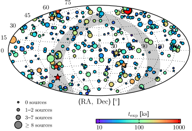
Figure 1.— Aitoff projection showing the distribution of NuSTAR serendipitous survey fields on the sky, in equatorial coordinates (R.A., decl.). The circle sizes correspond to the number of sources detected in a given field, and the colors correspond to the cumulative exposure time (per FPM) for a given field. The locations of the dedicated NuSTAR surveys in well-studied fields (COSMOS, ECDFS, EGS, GOODS-N, UDS, the Galactic center, and the Norma Arm), which are not included in the serendipitous survey, are marked with star symbols (with the colors representing the maximum unvignetted exposures). Also excluded from the serendipitous survey are NuSTAR fields containing bright targets (not shown on this figure; see Section 2.1). The gray area highlights the region $\pm 10$^∘ of the Galactic plane.

The fields have a cumulative exposure time of $20.4$ Ms. For comparison, the NuSTAR surveys of COSMOS and ECDFS have cumulative exposure times of $3.1$ Ms and $1.5$ Ms (C15 and M15, respectively). The serendipitous survey fields cover a wide range in individual exposure times (from $\sim 10$ ks to $1$ Ms), and have a median exposure of $28$ ks (these values correspond to a single NuSTAR FPM). For $76\%$ of the fields there is a single NuSTAR exposure, and for the remainder there are multiple (from two to $15$) exposures which are combined together for the science analyses (see Section 2.2).

An important contributor of fields to the NuSTAR serendipitous survey is the NuSTAR “snapshot survey” (Baloković et al. 2014; Baloković et al. 2017, in prep.), a dedicated NuSTAR program targetting Swift BAT-selected AGNs (the Swift BAT AGNs themselves are not included in the serendipitous survey, only the background regions of the NuSTAR observations). For this work we include $154$ snapshot survey fields observed during the first $40$ months of NuSTAR operation. These yield $21\%$ of the total serendipitous survey source detections, and make up a large fraction of the survey area (accounting for $47\%$ of the fields incorporated, in total).

2.2. Data processing

For data reduction, we use HEASoft v. 6.15, the NuSTAR Data Analysis Software (NuSTARDAS) v. 1.3.0, and CIAO v. 4.8. For each of the $510$ obsIDs incorporated in the survey, the raw, unfiltered event files for FPMA and FPMB were processed using the nupipeline program to yield calibrated, cleaned event files. For source detection and photometry (see Sections 2.3 and 2.4), we adopt the observed-frame energy bands which have been utilized for the NuSTAR extragalactic survey programme in general, and other recent NuSTAR studies: $3$–$8$, $3$–$24$, and $8$–$24$ keV (hereafter referred to as the soft, full, and hard bands; e.g., Alexander et al., 2013; Luo et al., 2014; Aird et al., 2015b; Lansbury et al., 2015; Harrison et al., 2016). To produce individual energy band images from the NuSTAR event lists we used the CIAO program dmcopy (Fruscione et al., 2006).

To produce exposure maps, which account for the natural dither of the observatory and regions of lower sensitivity (e.g., chip gaps), we follow the procedure outlined in detail in Section 2.2.3 of M15. Vignetting in the optics results in a decrease in the effective exposure with increasing distance from the optical axis. We produce both vignetting-corrected and non-vignetting-corrected exposure maps. The former allow us to determine the effective exposure at source positions within the FoV and correctly determine count rates, while the latter are more appropriate for the scaling of background counts since the NuSTAR aperture background component dominates the background photon counts at $\lesssim 30$ keV (e.g., Wik et al., 2014).

In order to increase sensitivity, we perform source detection (see Section 2.3) and photometry (see Section 2.4) on the coadded FPMA+FPMB (hereafter “A+B”) data, produced by combining the FPMA and FPMB science data with the HEASoft package ximage. For fields with multiple obsIDs, we use ximage to combine the data from individual observations, such that each field has a single mosaic on which source detection and photometry are performed.

2.3. Source detection

In general, the source-detection procedure follows that adopted in the dedicated blank-field surveys (e.g., see C15 and M15). A significant difference with the serendipitous survey, compared to the blank-field surveys, is the existence of a science target at the FoV aim-point. We account for the background contribution from such science targets by incorporating them in the background map generation, as described below. We also take two steps to exclude sources associated with the science target: (1) in cases where the target has an extended counterpart in the optical or IR bands (e.g., a low-redshift galaxy or galaxy cluster), we mask out custom-made regions which are conservatively defined to be larger than the extent of the counterpart in the optical imaging coverage (from the SDSS or DSS), accounting for spatial smearing of emission due to the NuSTAR PSF; (2) for all point-source detections with spectroscopic identifications, we assign an “associated” flag to those which have a velocity offset from the science target [$\Delta(cz)$] smaller than $5\%$ of the total science target velocity.

Here we summarize the source detection procedure, which is applied separately for each of the individual NuSTAR energy bands (soft, full, and hard) before the individual band source lists are merged to form the final catalog. For every pixel position across the NuSTAR image, a “false probability” is calculated to quantify the chance that the counts measured in a source detection aperture around that position are solely due to a background fluctuation. In this calculation we adopt a circular source detection aperture of radius $20\arcsec$, which is justified by the tight core of the NuSTAR PSF (FWHM$=18\arcsec$), and was also adopted for the dedicated blank-field surveys (e.g., C15; M15). To measure the background level at each pixel position, background counts are first measured from the NuSTAR image using an annular aperture of inner radius $45\arcsec$ and outer radius $90\arcsec$, centered on that position. These background counts are then re-scaled to the $20\arcsec$ source detection aperture according to the ratio of effective areas (as determined from non-vignetting-corrected exposure maps). This approach allows the local background to be sampled without significant contamination from the serendipitous source counts (since the background annulus has a relatively large inner radius). The background measurement also accounts for any contaminating photons from the aim-point science target which, due to the broad wings of the NuSTAR PSF, can contribute to the background (if the science target is comparatively bright and offset by $\lesssim 200^{\prime\prime}$ from the serendipitous source position). The Poisson false probability ($P_{\rm False}$) is assessed at each pixel, using the source and scaled background counts (e.g., Lehmer et al., 2005; Nandra et al., 2005; Laird et al., 2009), to yield a $P_{\rm False}$ map. From this map we exclude areas within $30\arcsec$ of the low-exposure ($<10\%$ of the maximum exposure) peripheral regions close to the FoV edge, where there is a steep drop-off in exposure and the background is poorly characterized.

We then perform source detection on the $P_{\rm False}$ map to identify sources. For a full, detailed description of this source detection procedure we refer the reader to Section 2.3 of M15. In brief, the SExtractor algorithm (Bertin & Arnouts, 1996) is used to identify regions of each $P_{\rm False}$ map which fall below a threshold of $\log(P_{\rm False})<-6$ (the approximate average of the thresholds adopted for the NuSTAR-COSMOS and NuSTAR-ECDFS surveys; C15; M15), producing source lists for each individual energy band. The coordinates for each detected source are measured at the local minimum in $P_{\rm False}$. Finally, we merge the sources detected in the different energy bands to yield a final source list. To achieve this band-merging, the soft ($3$–$8$ keV) and hard ($8$–$24$ keV) band detected sources are matched to the full ($3$–$24$ keV) band source list using a matching radius of $35\arcsec$. The adopted NuSTAR source coordinates correspond to the position of the source in the full band, if there is a detection in this band. Otherwise the coordinates correspond to the soft band, if there is a detection in this band, or the hard band if there is no full or soft band detection. The analyses described below (e.g., photometry and multiwavelength counterpart matching) are performed using these adopted source coordinates. After the above source detection has been performed, we exclude any sources within $90\arcsec$ of the central science target position (for comparison, the half-power diameter of the NuSTAR PSF is $58\arcsec$).

To determine the overall sky coverage of the survey as a function of flux sensitivity, we sum the sensitivity curves for the $331$ individual fields. For each field the sensitivity curve is determined by calculating, for every point in the NuSTAR image (excluding the low-exposure peripheral regions), the flux limit corresponding to $\log(P_{\rm False})=-6$ (the detection threshold), given the background and exposure maps described above and the count-rate to flux conversion factors listed in Section 2.4. Figure 2 shows the total, summed sensitivity curves for the serendipitous survey, for the three main energy bands.

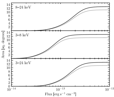
Figure 2.— Sky coverage (solid angle) of the NuSTAR serendipitous survey as a function of (aperture-corrected) flux sensitivity, for the three main energy bands. The black line shows the area curve for the full survey, and the gray line shows that for the survey regions outside the Galactic plane ($|b|>10$^∘).

Figure 3 shows the logarithmic version, compared to the other components of the NuSTAR extragalactic surveys program. The serendipitous survey has the largest solid angle coverage for most fluxes, and a similar areal coverage to the deepest blank-field survey (the NuSTAR-EGS survey) at the lowest flux limits. In both Figure 2 and Figure 3 we also show the area curves for the subset of the serendipitous survey which lies outside of the Galactic plane ($|b|>10$^∘) and is thus relatively free of Galactic sources. We note that the recent works of Aird et al. (2015b) and Harrison et al. (2016), which presented the luminosity functions and source number counts for the NuSTAR extragalactic survey program, only incorporated serendipitous survey fields at $|b|>20$^∘ (and at $\mathrm{decl.}>-5$^∘ for Aird et al. 2015b).

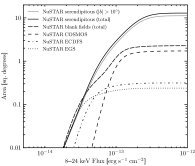
Figure 3.— Sky coverage (solid angle) of the NuSTAR serendipitous survey as a function of flux sensitivity, for the hard ($8$–$24$ keV) energy band, at which NuSTAR is uniquely sensitive. I.e., the sky coverage for which sources above a given hard band flux will be detected in the hard band. The black and gray solid lines show the area curves for the overall and the $|b|>10$^∘ serendipitous survey, respectively. We compare with the other completed components of the NuSTAR extragalactic surveys program, which include the following dedicated blank-field surveys: NuSTAR-COSMOS (dashed line; C15), NuSTAR-ECDFS (dash-dotted line; M15), and NuSTAR-EGS (dotted line; Aird et al., in prep.). The total area for these blank-field surveys (which are not included as part of the serendipitous survey) is shown as a long-dashed line.

2.4. Photometry

For each source detected using the above procedure we measure the net counts, count rates and fluxes, and for sources with spectroscopic redshifts we calculate rest-frame luminosities. For the aperture photometry, we adopt a circular aperture of $30\arcsec$ radius to measure the gross (i.e., source plus background) counts ($S$). The scaled background counts ($B_{\rm src}$) are determined using the same procedure as for the source detection (Section 2.3), and are subtracted from $S$ to obtain the net source counts ($S_{\rm net}$). The errors on $S_{\rm net}$ are computed as $1+\sqrt{S+0.75}$ ($84\%$ confidence level; e.g., Gehrels 1986). For sources undetected in a given band, upper limits for $S_{\rm net}$ are calculated using the Bayesian approach outlined in Kraft et al. (1991). To determine the net count rate, we divide $S_{\rm net}$ by the exposure time drawn from the vignetting-corrected exposure map (mean value within the $30^{\prime\prime}$ aperture).

Deblending is performed following the procedure outlined in detail in Section 2.3.2 of M15. In short, for a given source, the contributions from neighboring detections (within a $90\arcsec$ radius) to the source aperture counts are accounted for using knowledge of their separation and brightness. The false probabilities and photometric quantities (e.g., counts, flux) are all recalculated post-deblending, and included in the catalog in separate columns. Out of the total $498$ sources in the source catalog, only one is no longer significant (according to our detection threshold) post-deblending.

NuSTAR hard-to-soft band ratios ($\mathrm{BR}_{\mathrm{Nu}}$) are calculated as the ratio of the $8$–$24$ to $3$–$8$ keV count rates. For sources with full band counts of $S_{\rm net}>100$, and with a detection in at least one of the soft or hard bands, we derive an effective photon index ($\Gamma_{\rm eff}$); i.e., the spectral slope of a power law spectrum that is required to produce a given band ratio.

To measure fluxes, we convert from the deblended $30\arcsec$ count rates using the following conversion factors: $6.7\times 10^{-11}$, $9.4\times 10^{-11}$ and $13.9\times 10^{-11}$ $\mathrm{erg\ cm^{-2}\ cts^{-1}}$ for the soft, full and hard bands, respectively. These conversion factors were derived to account for the NuSTAR response, and assume an unabsorbed power-law with a photon index of $\Gamma_{\rm eff}=1.8$ (typical of AGN detected by NuSTAR; e.g., Alexander et al. 2013). The conversion factors return aperture-corrected fluxes; i.e., they are corrected to the $100\%$ encircled-energy fraction of the PSF. The general agreement between our NuSTAR fluxes and those from Chandra and XMM-Newton (see Section 3.1) indicates that the NuSTAR flux measurements are reliable. For sources with spectroscopic redshifts, we determine the rest-frame $10$–$40$ keV luminosity by extrapolating from a measured observed-frame flux, assuming a photon index of $\Gamma_{\rm eff}=1.8$. To ensure that the adopted observed-frame flux energy band corresponds to the rest-frame $10$–$40$ keV energy band, we use the observed-frame $8$–$24$ and $3$–$8$ keV bands for sources with redshifts of $z<1.35$ and $z\geq 1.35$, respectively. For cases with a non-detection in the relevant band (i.e., $8$–$24$ or $3$–$8$ keV), we instead extrapolate from the full band ($3$–$24$ keV).

2.5. The source catalog

The serendipitous survey source catalog is available as an electronic table. In Section A.1 we give a detailed description of the $106$ columns that are provided in the catalog. In total, the catalog contains $497$ sources which are significantly detected (according to the definition in Section 2.3) post-deblending, in at least one energy band. Table 2 provides source detection statistics, broken down for the different combinations of energy bands, and the number of sources with spectroscopic redshift measurements.

Table 2Source statistics for the NuSTAR serendipitous survey

Band	$N$	$N_{z}$
(1)	(2)	(3)
Any band	$497$	$276$
F + S + H	$104$ ($21\%$)	$77$
F + S	$116$ ($23\%$)	$82$
F + H	$35$ ($7\%$)	$21$
S + H	$0$ ($0\%$)	$0$
F	$165$ ($33\%$)	$77$
S	$53$ ($11\%$)	$16$
H	$24$ ($5\%$)	$3$

Notes. (1): F, S, and H refer to sources detected in the full ($3$–$24$ keV), soft ($3$–$8$ keV), and hard ($8$–$24$ keV) energy bands. E.g.: “F + H” refers to sources detected in the full and hard bands only, but not in the soft band; and “S” refers to sources detected exclusively in the soft band. (2): The number of sources detected post-deblending, for a given band or set of bands. (3): The number of sources with spectroscopic redshift measurements.

In addition to the primary source detection approach (Section 2.3), which has been used to generate the above main catalog, in Section A.6 we provide a “secondary catalog” containing sources that do not appear in the main catalog (for reasons described therein). However, all results in this work are limited to the main catalog only (the secondary catalog is thus briefer in content).

3. The Multiwavelength Data

The positional accuracy of NuSTAR ranges from $\approx 8^{\prime\prime}$ to $\approx 20^{\prime\prime}$, depending on the source brightness (the latter is demonstrated in the following section). For matching to unique counterparts at other wavelengths (e.g., optical and IR), a higher astrometric accuracy is required, especially toward the Galactic plane where the sky density of sources increases dramatically. We therefore first match to soft X-ray (Chandra, XMM-Newton, and Swift XRT) counterparts, which have significantly higher positional accuracy (Section 3.1), before proceeding to identify optical and IR counterparts (Section 3.2), and undertaking optical spectroscopy (Section 3.3)

3.1. Soft X-ray counterparts

The NuSTAR serendipitous survey is mostly composed of fields containing well-known extragalactic and Galactic targets. This means that the large majority of the serendipitous survey sources also have lower-energy (or “soft”) X-ray coverage from Chandra, XMM-Newton, or Swift XRT, thanks to the relatively large FoVs of these observatories. In addition, short-exposure coordinated Swift XRT observations have been obtained for the majority of the NuSTAR observations. Overall, $81\%$ ($401/497$) of the NuSTAR detections have coverage with Chandra or XMM-Newton, and this increases to $99\%$ ($493/497$) if Swift XRT coverage is included. Only $1\%$ ($4/497$) lack any form of coverage from all of these three soft X-ray observatories.

We crossmatch with the third XMM-Newton serendipitous source catalog (3XMM; Watson et al. 2009; Rosen et al. 2016) and the Chandra Source Catalog (CSC; Evans et al. 2010) using a $30\arcsec$ search radius from each NuSTAR source position; the errors in the source matching are dominated by the NuSTAR positional uncertainty (as quantified below). Based on the sky density of X-ray sources with $f_{\rm 2-10keV}\gtrsim 10^{-14}$ erg s^-1 cm^-2 found by Mateos et al. (2008; for $|b|>20$^∘ sources in the XMM-Newton serendipitous survey), we estimate that the $30\arcsec$ radius matching results in a typical spurious match fraction of $\approx 7\%$ for this flux level and latitude range. Overall, we find multiple matches for $\approx 20\%$ of the cases where there is at least one match. In these multiple match cases we assume that the 3XMM or CSC source with the brightest hard-band ($4.5$–$12$ keV and $2$–$7$ keV, respectively) flux is the correct counterpart. We provide the positions and Chandra/XMM-Newton $3$–$8$ keV fluxes ($F_{\mathrm{soft}}$) for these counterparts in the source catalog (see Section A.1). To assess possible flux contributions from other nearby Chandra/XMM-Newton sources, we also determine the total combined flux of all 3XMM or CSC sources contained within the $30\arcsec$ search aperture ($F_{\mathrm{soft}}^{\mathrm{30}}$). For the $284$ sources which are successfully matched to 3XMM or CSC, $29$ ($10\%$) have $F_{\mathrm{soft}}^{\mathrm{30}}$ values which exceed $F_{\mathrm{soft}}$ by a factor of $>1.2$, and there are only four cases where this factor is $>2$. In other words, there are few cases where additional nearby X-ray sources appear to be contributing substantially to the NuSTAR detected emission.

In addition to the aforementioned catalog matching, we identify archival Chandra, XMM-Newton and Swift XRT data that overlap in sky coverage with the NuSTAR data. Using these archival data sets, we manually identify and measure positions for soft X-ray counterparts which are not already included in the 3XMM and CSC catalogs. For Chandra we process the archival data using chandra_repro, for XMM-Newton we analyze data products from the Pipeline Processing System, and for Swift XRT we use screened event files (as provided on HEASARC). We perform source detection on the archival soft X-ray ($\approx 0.5$–$8$ keV) counts images using the CIAO source detection algorithm $\mathtt{wavdetect}$ (Freeman et al., 2002), which identifies $111$ new soft X-ray counterparts. $88\%$ of these have high detection significances (false probabilities of $<10^{-6}$), and $12\%$ have moderate detection significances (false probabilities of $10^{-6}$–$10^{-4}$).

In total, soft X-ray counterparts are successfully identified for $79\%$ ($395/497$) of the NuSTAR detections: $284$ are existing counterparts in the 3XMM and CSC catalogs, with $269$ and $82$ counterparts from the individual 3XMM and CSC catalogs, respectively. Of the remaining $213$ NuSTAR detections that lack 3XMM and CSC counterparts, we have manually identified soft X-ray counterparts in archival data (using $\mathtt{wavdetect}$ as described above) for $111$ sources, of which $27$, $60$, and $24$ are from Chandra, Swift XRT, and XMM-Newton data, respectively. In addition, we manually determine new Chandra positions for $12$ sources which appear in 3XMM and not CSC, but have Chandra coverage, thus improving the X-ray position constraints for these sources. For four of these sources, the newly measured Chandra positions were obtained through our own Chandra observing program aimed at localizing the X-ray emission for Galactic-candidate NuSTAR serendipitous sources (Tomsick et al., in prep.). For the soft X-ray counterparts which are detected with multiple soft X-ray observatories, we adopt the position with the highest accuracy: for $31\%$ ($121/395$) the adopted position is from Chandra, which has the best positional accuracy; for $54\%$ ($214/395$) the adopted position is from XMM-Newton; and for $15\%$ ($60/395$) the adopted counterpart is from Swift XRT.

Overall, $21\%$ ($102/497$) of the NuSTAR detections lack soft X-ray counterparts. This can largely be explained as a result of insufficient-depth soft X-ray coverage, or zero coverage. However, for the sources with sufficient-depth soft X-ray coverage this may indicate either a spurious NuSTAR detection, a transient detection, or the detection of an unidentified contaminating feature such as stray light (e.g., Mori et al. 2015). We estimate that there are $34$ (out of $102$) such sources, that lack a soft X-ray counterpart but have sufficiently deep soft X-ray data (from Chandra or XMM-Newton) that we would expect a detection (given the NuSTAR source flux in the overlapping $3$–$8$ keV band). We retain these sources in the sample, but note that their inclusion (or exclusion) has a negligible impact on the results presented herein which are primarily based on the broader subsample with successful counterpart identifications and spectroscopic redshift measurements.

The upper panel of Figure 4 shows the distribution of positional offsets (in R.A. and decl.) for the NuSTAR sources relative to their soft X-ray (Chandra, XMM-Newton, and Swift XRT) counterparts. We find no evidence for systematic differences in the astrometry between observatories, since the mean positional offsets are all consistent with zero: the mean values of $\Delta\mathrm{RA}\cdot\cos(\mathrm{Dec})$ and $\Delta\mathrm{Dec}$ are $0.41\pm 1.45^{\prime\prime}$ and $0.18\pm 1.28^{\prime\prime}$ for Chandra, $-0.19\pm 1.11^{\prime\prime}$ and $0.50\pm 0.95^{\prime\prime}$ for XMM-Newton, and $-0.34\pm 1.97^{\prime\prime}$ and $1.70\pm 2.09^{\prime\prime}$ for Swift XRT.

The lower panel of Figure 4 shows the radial separation (in arcseconds) of NuSTAR sources from their well-localized soft X-ray counterparts (for those sources with Chandra or XMM-Newton counterparts) as a function of $P_{\rm False}$, thus illustrating the positional accuracy of NuSTAR as a function of source-detection significance. To reliably assess the positional accuracy of NuSTAR, we limit this particular analysis to sources with unique matches at soft X-ray energies, and thus with higher likelihoods of being correctly matched. Assuming zero uncertainty on the Chandra and XMM-Newton positions, the $90\%$ confidence limit on the NuSTAR positional uncertainty is $22\arcsec$ for the least-significant detections, and $14\arcsec$ for the most-significant detections. If we instead only consider the Chandra positions, which are in general more tightly constrained (positional accuracy $\lesssim 1\arcsec$; e.g., see Section 3.2), then the inferred $90\%$ positional accuracy of NuSTAR improves to $20\arcsec$ and $12\arcsec$ for the least-significant and most-significant sources, respectively.

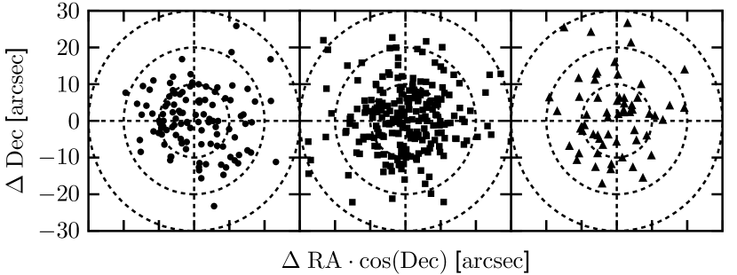
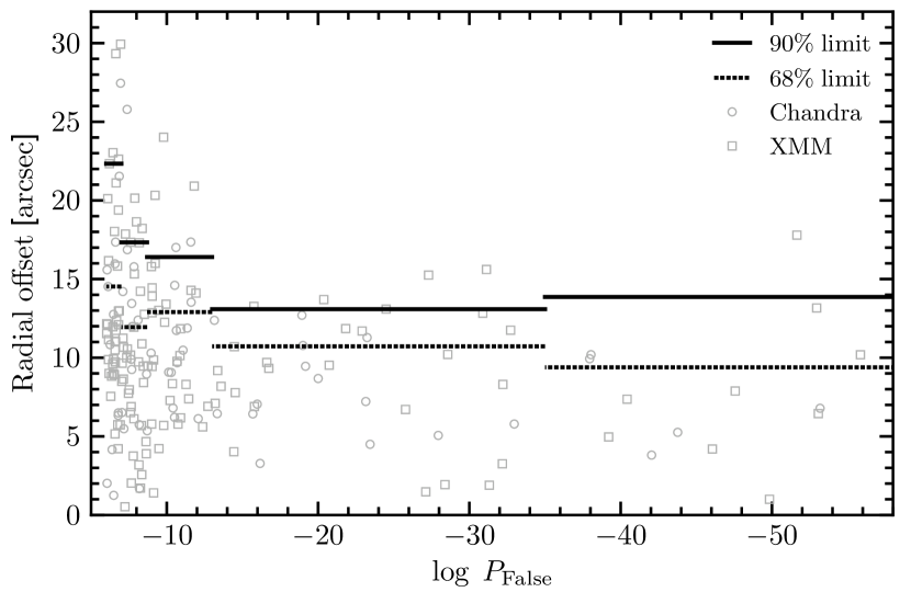
Figure 4.— Upper panel: astrometric offsets between the NuSTAR coordinates and lower-energy X-ray counterpart coordinates as identified with Chandra (circles, left panel), XMM-Newton (squares, center panel), and Swift XRT (triangles, right panel). Lower panel: the angular separation between NuSTAR and Chandra/XMM-Newton coordinates, as a function of $P_{\rm False}$ (source detection significance increases towards the right). The solid and dotted lines show the limits in angular offset enclosing $90\%$ and $68\%$ of sources, for bins in $P_{\rm False}$. Each bin contains $\approx 40$–$50$ sources, except the rightmost bin which contains $23$ sources (and extends beyond the x-axis upper limit, including all sources with $P_{\rm False}<-35$). This figure illustrates the positional accuracy of NuSTAR as a function of source significance.

Figure 5 compares the $3$–$8$ keV fluxes, as measured by NuSTAR, with those measured by Chandra and XMM-Newton for the sources with 3XMM or CSC counterparts. The small flux corrections from the 3XMM and CSC energy bands ($4.5$–$12$ keV and $2$–$7$ keV, respectively) to the $3$–$8$ keV energy band are described in Section A.1. The majority of sources ($92\%$ and $89\%$ for Chandra and XMM-Newton, respectively) are consistent with lying within a factor of three of the 1:1 relation, given the uncertainties, and thus show reasonable agreement between observatories. Given that the NuSTAR and the lower-energy X-ray observations are not contemporaneous, intrinsic source variability is expected to contribute to the observed scatter. A number of sources at the lowest X-ray fluxes lie above the relation, due to Eddington bias. This effect has been observed in the NuSTAR-ECDFS and NuSTAR-COSMOS surveys (M15; C15), and is predicted from simulations (C15).

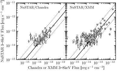
Figure 5.— Comparison of the NuSTAR and soft X-ray mission flux ($F_{\mathrm{soft}}$; from Chandra or XMM-Newton), at $3$–$8$ keV, for those serendipitous survey sources with matched CSC or 3XMM counterparts. The empty symbols show upper limits. The 1:1 relation is shown by a solid line, and the dotted lines show values a factor of three from this relation.

Two relatively high-flux 3XMM sources lie significantly below the 1:1 relation, suggesting that they have experienced a large decrease in flux (by a factor of $\gtrsim 5$). The first, NuSTAR J183452-0845.6, is a known Galactic magnetar for which the NuSTAR (2015) flux is lower than the XMM-Newton (2005 and 2011 combined) flux by a factor of $\approx 15$. This is broadly consistent with the known properties of the source, which varies in X-ray flux by orders of magnitude over multi-year timescales (e.g., Younes et al., 2012). The second outlying source is extragalactic in origin: NuSTAR J133311-3406.8 (hereafter J1333; $z=0.091$; $L_{\rm 10-40keV}=8\times 10^{42}$ erg s^-1). Our NTT (ESO New Technology Telescope) spectrum for J1333 reveals a NLAGN, with an apparently asymmetric, blue wing component to the H$\alpha$$+$[N II] complex, and our NTT $R$-band imaging shows a well-resolved, undisturbed host galaxy. Modeling the XMM-Newton ($14$ ks exposure; $\approx 1100$ EPIC source counts at $0.5$–$10$ keV) and NuSTAR ($17$ ks exposure; $\approx 75$ source counts at $3$–$24$ keV) spectra, the former of which precedes the latter by $\approx 9$ years, the X-ray spectral flux has decreased by a factor of $\approx 5$ in the energy band where the observatories overlap in sensitivity ($3$–$10$ keV). While this is an outlier, it is not unexpected to observe one AGN with this level of variability, given the range of AGN variability observed on decade timescales in deep $<10$ keV X-ray surveys such as CDFS (e.g., Yang et al., submitted). The variability could be due to a change in the intrinsic X-ray continuum, or the line-of-sight column density (e.g., Risaliti et al. 2005; Markowitz et al. 2014). However, it is not possible to place informative constraints on spectral shape variability of J1333, since the NuSTAR spectral shape is poorly constrained at $3$–$10$ keV ($\Gamma_{\rm eff}=1.2^{+1.3}_{-1.7}$). Deeper, simultaneous broad-band X-ray coverage would be required to determine whether a variation in spectral shape accompanies the relatively large variation in AGN flux. There is Swift XRT coverage contemporaneous with the 2014 NuSTAR data, but J1333 is undetected by Swift XRT. The Swift XRT flux upper limit is consistent with the NuSTAR flux, and is a factor of $\approx 4.2$ lower than the XMM-Newton flux (and thus in agreement with a factor of $\approx 5$ variation in the X-ray flux). This source represents the maximum variation in AGN flux identified in the survey.

3.2. IR and optical counterparts

Here we describe the procedure for matching between the $395$ (out of $497$) NuSTAR sources with soft X-ray counterparts (identified in Section 3.1), and counterparts at IR and optical wavelengths. The results from this matching are summarized in Table 3 (for the sources with Galactic latitudes of $|b|>10$^∘). We adopt matching radii which are a compromise between maximizing completeness and minimizing spurious matches, and take into account the additional uncertainty (at the level of $1^{\prime\prime}$) between the X-ray and the optical/IR positions. For Chandra positions we use a matching radius of $2.5\arcsec$, which is well-motivated based on the known behaviour of the positional uncertainty as a function of off-axis angle (the majority of NuSTAR serendipitous sources lie significantly off-axis) and source counts (e.g., Alexander et al. 2003; Lehmer et al. 2005; Xue et al. 2011). For Swift XRT positions we use a matching radius of $6\arcsec$, justified by the typical positional uncertainty (statistical plus systematic) which is at the level of $\approx 5.5\arcsec$ ($90\%$ confidence level; e.g., Moretti et al. 2006; Evans et al. 2014). For XMM-Newton positions we use a matching radius of $5\arcsec$, which is motivated by the typical positional uncertainties of X-ray sources in the XMM-Newton serendipitous survey (e.g., $\approx 4\arcsec$ at the $90\%$ confidence level for XMM-Newton bright serendipitous survey sources; Caccianiga et al. 2008).

Table 3Summary of the optical and IR counterpart matching statistics and photometric magnitudes

Catalog / Band	$N$	Fraction	$m_{\rm max}$	$m_{\rm min}$	$\bar{m}$	$\left<m\right>$
(1)	(2)	(3)	(4)	(5)	(6)	(7)
Total optical + IR	$290$	$87.9\%$	$\cdots$	$\cdots$	$\cdots$	$\cdots$
WISE (all)	$252$	$76.4\%$	$\cdots$	$\cdots$	$\cdots$	$\cdots$
WISE / W1	$249$	$75.5\%$	$18.4$	$7.8$	$15.3$	$15.5$
WISE / W2	$248$	$75.2\%$	$17.1$	$7.9$	$14.4$	$14.6$
WISE / W3	$194$	$58.8\%$	$13.3$	$4.5$	$11.2$	$11.4$
WISE / W4	$131$	$39.7\%$	$9.9$	$1.8$	$8.1$	$8.4$
Optical (all)	$249$	$75.5\%$	$\cdots$	$\cdots$	$\cdots$	$\cdots$
SDSS / $r$	$121$	$36.7\%$	$24.5$	$11.7$	$19.6$	$19.9$
USNOB1 / $R$	$198$	$60.0\%$	$20.9$	$10.5$	$18.5$	$19.1$

Notes. Summary of the optical and IR counterpart matching for the $330$ NuSTAR serendipitous survey sources with high Galactic latitudes ($|b|>10$^∘) and soft X-ray telescope (Chandra, Swift XRT, or XMM-Newton) counterpart positions (see Section 3.2). (1): The catalog and photometric band (where magnitude statistics are provided). (2): The number of the NuSTAR sources successfully matched to a counterpart in a given catalog. For the WISE all-sky survey catalog, this is broken down for the four photometric WISE bands. (3): The fraction of the NuSTAR sources which are matched. (4): The maximum (i.e., faintest) magnitude for the counterparts in a given catalog and photometric band. (5): The minimum (i.e., brightest) magnitude. (6): The mean magnitude. (7): The median magnitude.

To identify IR counterparts, we match to the WISE all-sky survey catalog (Wright et al., 2010). Of the $395$ sources with soft X-ray counterparts, $274$ ($69\%$) have WISE matches. In $100\%$ of these cases there is a single unique WISE match (detected in at least one WISE band). To identify optical counterparts, we match to the SDSS DR7 catalog (York et al., 2000) and the USNOB1 catalog (Monet et al. 2003). If both contain matches, we adopt optical source properties from the former catalog. Of the $395$ sources with soft X-ray counterparts, $252$ ($64\%$) have a match in at least one of these optical catalogs: $121$ have an SDSS match and $131$ without SDSS matches have a USNOB1 match. In $77\%$ ($193/252$) of cases there is a single optical match. In the case of multiple matches within the search radius we adopt the closest source. Figure 6 shows the distribution of astrometric offsets between the soft X-ray counterparts and the WISE and optical (SDSS and USNOB1) counterparts.

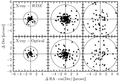
Figure 6.— Astrometric offsets between the soft X-ray counterpart coordinates and the WISE (top row) and optical (bottom row) coordinates. The soft X-ray counterparts are from Chandra (left column), XMM-Newton (middle column) and Swift XRT (right column). The dashed circles correspond to the search radii for each telescope ($2.5\arcsec$, $5\arcsec$ and $6\arcsec$ for Chandra, XMM-Newton and Swift XRT, respectively).

For Galactic latitudes of $|b|>10$^∘, which we focus on for the analysis of NuSTAR serendipitous survey source properties (Section 4), the spurious matching fractions are low ($\lesssim 10\%$; see Section A.3).

For the $143$ (out of $395$) soft X-ray counterparts without SDSS and USNOB1 matches, we determine whether there are detections within the existing optical coverage, which is primarily photographic plate coverage (obtained through the DSS) but also includes dedicated $R$-band and multi-band imaging from our own programs with the ESO-NTT (EFOSC2) and ESO-2.2m (GROND), respectively. This identifies an additional $33$ optical counterparts. For the $110$ non-detections, we estimate $R$-band magnitude lower limits from the data (all cases have coverage, at least from photographic plate observations). These optical non-detections do not rule out follow-up spectroscopy; for $21$ of them we have successfully performed optical spectroscopy, obtaining classifications and redshifts, either by identifying an optical counterpart in pre-imaging or by positioning the spectroscopic slit on a WISE source within the X-ray error circle. In Figure 7 we show histograms of the WISE and $R$-band magnitudes for the NuSTAR sources with soft X-ray counterparts.

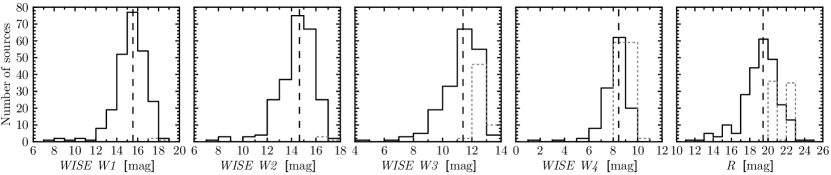
Figure 7.— Distributions of the MIR and optical magnitudes for the NuSTAR serendipitous survey sources with high Galactic latitudes ($|b|>10$^∘) and soft X-ray telescope (Chandra, Swift XRT, or XMM-Newton) counterparts. Left four panels: magnitude distributions for the four photometric WISE bands, for the sources with successful matches to the WISE all-sky survey catalog. For each band, the solid line shows the magnitude distribution for detected sources, the dashed line marks the median magnitude of the detections, and the dotted line shows the distribution of magnitude lower limits for sources undetected in that band (but detected in other bands). Right panel: the $R$-band magnitudes (primarily from matching to the SDSS and USNOB1 catalogs) for all the sources.

For the $102$ (out of $497$) sources without soft X-ray counterparts, the X-ray positional error circle (from NuSTAR) is comparatively large (see Section 3.1), so unique counterparts cannot be identified with high confidence. To identify possible counterparts for these sources, for the purposes of optical spectroscopic followup, we consider the properties of nearby WISE sources. Matching to the WISE all-sky survey, we identify AGN candidates within a $25^{\prime\prime}$ radius of the NuSTAR position, using the following two criteria: a WISE color of $W{\rm 1}$–$W{\rm 2}>0.8$ (and $W{\rm 2}<15$; Vega mag; Stern et al. 2012) or a $W{\rm 4}$ band detection. The WISE $W{\rm 1}$, $W{\rm 2}$, $W{\rm 3}$, and $W{\rm 4}$ bands are are centered at $3.4$ µm, $4.6$ µm, $12$ µm, and $22$ µm, respectively. We limit this matching to the $85$ (out of $102$) sources at Galactic latitudes above $|b|=10$^∘. Given the sky densities of WISE sources which satisfy these criteria, ($\approx 46$ deg^-2 and $\approx 730$ deg^-2, respectively, for $|b|>10$^∘), the probabilities of chance matches are $\approx 1\%$ and $\approx 11\%$, respectively. Where multiple such WISE sources are identified, we prioritize those which satisfy both criteria, then those which satisfy the former criterion. For $24$ (out of $102$) of these sources there is a WISE AGN candidate within the NuSTAR error circle, the position of which we match to optical counterparts. The optical and IR counterparts identified in this manner (for NuSTAR sources without soft X-ray counterparts) are primarily used for the purposes of undertaking spectroscopic followup (Section 3.3), and we exclude them from our analysis of the IR properties of the NuSTAR serendipitous survey AGNs (Section 4.3), to avoid biasing the results. For the remaining $78$ (out of $102$) sources at $|b|<10$^∘ or without matches to WISE AGN candidates, we use the available $R$-band information to obtain magnitude constraints: in cases where there is at least one optical source within the NuSTAR error circle, we adopt the lowest (i.e., brightest) $R$-band magnitude as a lower limit; and in cases with no optical source within the NuSTAR error circle, we adopt the magnitude limit of the imaging data.

For a large fraction of the sources discussed in this section, the spectroscopic followup (Section 3.3) shows evidence for an AGN, which provides additional strong support for correct counterpart identification (given the low sky density of AGNs). Furthermore, the optical and IR photometric properties of the NuSTAR serendipitous survey counterparts are in agreement with AGNs (see Sections 4.2.1 and 4.3.1).

3.3. Optical Spectroscopy

Optical identifications and source redshifts, obtained through spectroscopy, are a prerequisite to the measurement of intrinsic source properties such as luminosity and the amount of obscuration. A small fraction ($\approx 11\%$; $57/497$) of the NuSTAR serendipitous survey sources have pre-existing spectroscopic coverage, primarily from the SDSS. However, the majority ($\approx 89\%$) of the serendipitous survey sources do not have pre-existing spectroscopy. For that reason, we have undertaken a campaign of dedicated spectroscopic followup in the optical–IR bands (Section 3.3.1), obtaining spectroscopic identifications for a large fraction ($56\%$) of the total sample. For the high Galactic latitude ($|b|>10$^∘) samples selected in individual bands, this has resulted in a spectroscopic completeness of $\approx 70\%$. The analysis of and classifications obtained from these new spectroscopic data, and those from pre-existing spectroscopy, are described in Section 3.3.2.

3.3.1 Dedicated followup campaign

Since NuSTAR performs science pointings across the whole sky, a successful ground-based followup campaign requires the use of observatories at a range of geographic latitudes, and preferably across a range of dates throughout the sidereal year. This has been achieved through observing programmes with, primarily, the following telescopes over a multi-year period: the Hale Telescope at Palomar Observatory ($5.1$ m; Decl. $\gtrsim-21$^∘; PIs F. A. Harrison and D. Stern); Keck I and II at the W. M. Keck Observatory ($10$ m; $-35$^∘ $\lesssim$ Decl. $\lesssim 75$^∘; PIs F. A. Harrison and D. Stern); the New Technology Telescope (NTT) at La Silla Observatory ($3.6$ m; Decl. $\lesssim 25$^∘; PI G. B. Lansbury); the Magellan I (Baade) and Magellan II (Clay) Telescopes at Las Campanas Observatory ($6.5$ m; Decl. $\lesssim 25$^∘; PIs E. Treister and F. E. Bauer); and the Gemini-South observatory ($8.1$ m; Decl. $\lesssim 25$^∘; PI E. Treister). Table 4 provides a list of the observing runs undertaken. In each case we provide the observing run starting date (UT), number of nights, telescope, instrument, and total number of spectroscopic redshifts obtained for NuSTAR serendipitous survey sources.

Table 4Chronological list of ground-based observing runs for spectroscopic followup of the NuSTAR serendipitous survey

Run ID	UT start date	Telescope	Instrument	Spectra
(1)	(2)	(3)	(4)	(5)
1	2012 Oct 10	Palomar	DBSP	$1$
2	2012 Oct 13	Keck	DEIMOS	$1$
3	2012 Nov 09	Keck	LRIS	$1$
4	2012 Nov 20	Palomar	DBSP	$2$
5	2012 Dec 12	Gemini-South	GMOS	$1$
6	2013 Jan 10	Keck	LRIS	$1$
7	2013 Feb 12	Palomar	DBSP	$2$
8	2013 Mar 11	Palomar	DBSP	$6$
9	2013 Jul 07	Palomar	DBSP	$2$
10	2013 Oct 03	Keck	LRIS	$9$
11	2013 Dec 05	Magellan	MagE	$2$
12	2013 Dec 10	Keck	DEIMOS	$6$
13	2014 Feb 22	Palomar	DBSP	$4$
14	2014 Apr 22	Palomar	DBSP	$6$
15	2014 Jun 25	Keck	LRIS	$12$
16	2014 Jun 30	NTT	EFOSC2	$8$
17	2014 Jul 21	Palomar	DBSP	$3$
18	2014 Sep 25	Magellan	MagE	$5$
19	2014 Oct 20	Keck	LRIS	$4$
20	2014 Dec 23	Palomar	DBSP	$4$
21	2015 Feb 17	Palomar	DBSP	$5$
22	2015 Mar 14	NTT	EFOSC2	$17$
23	2015 Mar 18	Magellan	IMACS	$6$
24	2015 May 19	NTT	EFOSC2	$14$
25	2015 Jun 09	Palomar	DBSP	$1$
26	2015 Jun 15	Palomar	DBSP	$1$
27	2015 Jul 17	Keck	LRIS	$3$
28	2015 Jul 21	Palomar	DBSP	$4$
29	2015 Aug 09	Palomar	DBSP	$6$
30	2015 Aug 12	Keck	LRIS	$6$
31	2015 Dec 04	Keck	LRIS	$28$
32	2015 Dec 06	NTT	EFOSC2	$25$
33	2016 Jan 11	Palomar	DBSP	$8$
34	2016 Feb 05	Palomar	DBSP	$2$
35	2016 Feb 08	Magellan	MagE	$6$
36	2016 Feb 13	Keck	LRIS	$17$
37	2016 Jul 05	Keck	LRIS	$10$
38	2016 Jul 10	Palomar	DBSP	$6$

Notes. (1): ID assigned to each observing run. (2): Observing run start date. (3) and (4): The telescope and instrument used. (5): The number of spectra from a given observing run which have been adopted, in this work, as the analysed optical spectrum for a NuSTAR serendipitous survey source. These correspond to the individual sources listed in Table LABEL:specTable of Section A.2, and are primarily ($\approx 93\%$) sources with successful redshift measurements and spectroscopic classifications. These source numbers exclude the $35$ sources in the secondary catalog for which we have obtained new spectroscopic identifications (see Section A.6).

The total number of sources with spectroscopic redshift measurements and classifications is $276$. The large majority of spectroscopic identifications in the northern hemisphere were obtained using a combination of Palomar and Keck, with the former being efficient for brighter targets and the latter for fainter targets. These account for $51\%$ ($141/276$) of the spectroscopically identified sample. Similarly, for the southern hemisphere the majority of spectroscopic identifications were obtained using the ESO NTT while complementary Magellan observations were used to identify the fainter optical sources. These account for $28\%$ ($76/276$) of the overall spectroscopically identified sample.

Conventional procedures were followed for spectroscopic data reduction, using IRAF routines. Spectrophotometric standard star observations, from the same night as the science observations, were used to flux calibrate the spectra.

3.3.2 Spectral Classification and Analysis

All flux-calibrated optical spectra from this work are provided in Section A.2. For our instrument setups, the typical observed-frame wavelength range covered is $\lambda\approx 3500$–$9000$Å. At lower redshifts, for example $z=0.3$, this results in coverage for the following emission lines common to AGNs and quasars: Mg II $\lambda 2800$, [Ne V] $\lambda 3346$ and $\lambda 3426$, [O II] $\lambda 3728$, [Ne III] $\lambda 3869$, H$\mathrm{\delta}$ $\lambda 4102$, H$\mathrm{\gamma}$ $\lambda 4340$, H$\mathrm{\beta}$ $\lambda 4861$, [O III] $\lambda 4959$ and $\lambda 5007$, [O I] $\lambda 6300$ and $\lambda 6364$, [N II] $\lambda 6548$ and $\lambda 6584$, H$\mathrm{\alpha}$ $\lambda 6563$, and [S II] $\lambda 6716$ and $\lambda 6731$. At higher redshifts, for example $z=2$, the lines covered are: Ly$\mathrm{\alpha}$ $\lambda 1216$, Si IV $\lambda 1398$, C IV $\lambda 1549$, He II $\lambda 1640$, C III] $\lambda 1909$, C II] $\lambda 2326$, and Mg II $\lambda 2800$.

To measure spectroscopic redshifts, we identify emission and absorption lines, and measure their observed-frame wavelengths using Gaussian profile fitting. To determine the redshift solution, we crossmatch the wavelength ratios of the identified lines with a look-up table of wavelength ratios based on the emission and absorption lines observed in AGN and galaxy spectra. The final, precise redshift measurement is then obtained from the Gaussian profile fit to the strongest line. For the large majority of cases there are multiple lines detected, and there is only one valid redshift solution. The lines identified for each individual NuSTAR source are tabulated in Section A.2. There are only five sources where the redshift is based on a single line identification (marked with “quality B” flags in Section A.2). For four of these, the single emission line detected is identified as Mg II $\lambda 2800$. In all cases this is well justified: Mg II is a dominant broad line in quasar spectra, and there is a relatively large separation in wavelength between the next strong line bluewards of Mg II (C III] $\lambda 1909$) and that redwards of Mg II (H$\mathrm{\beta}$ $\lambda 4861$). This means that Mg II can be observed in isolation for redshifts of $z\sim 0.8$ in cases where our wavelength coverage is slightly narrower than usual, or if the other lines (e.g., C III] and H$\mathrm{\beta}$) are below the detection threshold. Mg II can also be clearly identifiable in higher $S/N$ data due to the shape of the neighboring Fe II pseudo-continuum.

We perform optical classifications visually, based on the spectral lines observed. For the extragalactic sources with available optical spectra and with identified lines ($253$ sources), emission lines are detected for all but one source (where multiple absorption lines are identified). Both permitted emission lines (e.g., the Balmer series and Mg II) and forbidden (e.g., [O III] and [N II]) emission lines are identified for $183$ (out of $253$) sources. For these sources, if any permitted line is broader than the forbidden lines we assign a BLAGN classification, otherwise we assign a NLAGN classification. There are $58$ (out of $253$) sources where only permitted (or semi-forbidden) emission lines are identified. For the majority of these ($56$ sources) the line profiles are visually broad, and we assign a BLAGN classification (these sources predominantly lie at higher redshifts, with $51$ at $z\gtrsim 1$, and have quasar-like continuum-dominated spectra). For $24$ sources where there is a level of ambiguity as to whether the permitted lines are broad or not, we append the optical classification (i.e., “NL” or “BL” in Table LABEL:specTable) with a “?” symbol. For the remaining $11$ sources (out of $253$) with only forbidden line detections, and the single source with absorption line detections only, we assign NLAGN classifications.

In total we have spectroscopic classifications for $276$ of the NuSTAR serendipitous survey sources, including the $253$ extragalactic sources mentioned above, an additional BL Lac type object, $16$ Galactic ($z=0$) objects, and six additional (BLAGN and NLAGN) classifications from the literature. $222$ of these classifications were assigned using data from the dedicated observing runs (Table 4), and $54$ using existing data (primarily SDSS) or literature. Considering the total classified sample, the majority of the sources ($162$, or $58.7\%$) are BLAGNs, $97$ ($35.1\%$) are NLAGNs, one ($0.4\%$) is a BL Lac type object, and the remaining $16$ ($5.8\%$) are Galactic objects (e.g., cataclysmic variables and high mass X-ray binaries). Tomsick et al. (in prep.) will present a detailed analysis of the Galactic subsample. The current spectroscopic completeness (i.e., the fraction of sources with successful spectroscopic identifications) is $\approx 70\%$ for the overall serendipitous survey (for the $|b|>10$^∘ individual band-selected samples), although the completeness is a function of X-ray flux (see Section 4.2).

In Table LABEL:specTable (see Section A.2) we provide the following for all NuSTAR serendipitous survey sources with optical spectra: the spectroscopic redshift, the optical classification, the identified emission and absorption lines, individual source notes, and the observing run ID (linking to Table 4).

4. Results and Discussion

Here we describe the properties of the NuSTAR serendipitous survey sources, with a focus on the high energy X-ray (Section 4.1), optical (Section 4.2) and infrared (Section 4.3) wavelength regimes. We compare and contrast with other relevant samples, including: the blank-field NuSTAR surveys in well-studied fields (COSMOS and ECDFS); non-survey samples of extreme objects targetted with NuSTAR; the Swift BAT all-sky survey, one of the most sensitive high energy X-ray surveys to precede NuSTAR; and lower energy ($<10$ keV; e.g., Chandra and XMM-Newton) X-ray surveys.

4.1. X-ray properties

4.1.1 Basic NuSTAR properties

Overall there are $497$ sources with significant detections (post-deblending) in at least one band. Section 2.5 details the source-detection statistics, broken down by energy band. In the $8$–$24$ keV band, which is unique to NuSTAR amongst focusing X-ray observatories, there are $163$ detections, i.e. $33\%$ of the sample. The NuSTAR-COSMOS and NuSTAR-ECDFS surveys found fractions of $8$–$24$ keV detected sources which are consistent with this: $35\%$ ($32/91$ sources; C15) and $39\%$ ($19/49$ sources post-deblending; M15), respectively.

The net (cleaned, vignetting-corrected) exposure times per source ($t_{\rm net}$; for the combined FPMA+B data) have a large range, from $10$–$1500$ ks, with a median of $60$ ks. For the $3$–$8$, $8$–$24$, and $3$–$24$ keV bands, the lowest net source counts ($S_{\rm net}$) for sources with detections in these bands are $12$, $15$, and $18$, respectively. The highest $S_{\rm net}$ values are $9880$, $5853$, and $15693$, respectively, and correspond to one individual source NuSTAR J043727–4711.5, a BLAGN at $z=0.051$. The median $S_{\rm net}$ values are $56$, $62$, and $75$, respectively. The count rates range from $0.17$–$52$, $0.11$–$36$, and $0.13$–$94$ ks^-1, respectively, and the median count rates are $0.77$, $0.84$, and $1.1$ ks^-1, respectively.

Figure 8 shows the distribution of fluxes for the full sample, for each energy band. The distributions for detected and undetected sources (for a given band) are shown separately. For sources which are detected in the $3$–$8$, $8$–$24$, and $3$–$24$ keV bands, the faintest fluxes measured are $1.17$, $1.53$, and $1.22\times 10^{-14}$ erg s^-1 cm^-2, respectively. The brightest fluxes are $3.5$, $5.0$, and $8.8\times 10^{-12}$ erg s^-1 cm^-2, respectively, and correspond to one individual source NuSTAR J075800+3920.4, a BLAGN at $z=0.095$. The median fluxes are $5.2$, $11.6$, and $10.5\times 10^{-14}$ erg s^-1 cm^-2, respectively. The dynamic range of the serendipitous survey exceeds the other NuSTAR extragalactic survey components. For comparison, the blank-field ECDFS and COSMOS components span $3$–$24$ keV flux ranges of $\approx(2$–$10)$ and $(5$–$50)\times 10^{-14}$ erg s^-1 cm^-2, respectively (C15 and M15). The serendipitous survey pushes to fluxes (both flux limits and median fluxes) $\sim$ two orders of magnitude fainter than those achieved by previous-generation hard X-ray observatories such as Swift BAT (e.g., Baumgartner et al., 2013) and INTEGRAL (e.g., Malizia et al., 2012).

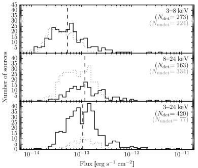
Figure 8.— Flux distributions in the soft, hard, and full energy bands (top, middle, and bottom panels, respectively) for the NuSTAR serendipitous survey sample. For each band, the solid line shows the flux distribution for sources independently detected in that band (the number of these sources, $N_{\rm det}$, is shown in black font), and the median flux of the detected sources is marked by a dashed line. For each band, the dotted line shows the distribution of flux upper limits for sources undetected in that band, but independently detected in at least one other band (the number of these sources, $N_{\rm undet}$, is shown in grey font).

4.1.2 Band ratios

Figure 9.— The NuSTAR $8$–$24$ to $3$–$8$ keV band ratio ($\mathrm{BR}_{\mathrm{Nu}}$) versus full-band ($3$–$24$ keV) count rate for the full NuSTAR serendipitous survey sample. Constrained $\mathrm{BR}_{\mathrm{Nu}}$ values are shown in black, and those with upper or lower limits are shown in gray. The dotted horizontal lines indicate spectral slopes ($\Gamma_{\rm eff}$) to which the band ratios correspond. The overplotted red circles show numerical means (binning in full-band count rate), for a subset of extragalactic sources with $\log(P_{\rm False})<-14$. The overplotted blue triangles show “stacked” means obtained from summing the net count-rates of all sources, including non-detections, and bootstrapping errors.

Figure 9 shows the $8$–$24$ to $3$–$8$ keV band ratios ($\mathrm{BR}_{\mathrm{Nu}}$) for the full sample of NuSTAR serendipitous survey sources, as a function of full-band ($3$–$24$ keV) count rate. In order to examine the results for extragalactic sources only, we remove sources which are spectroscopically confirmed as having $z=0$ (see Section 3.3) and exclude sources with Galactic latitudes below $|b|=10$^∘, for which there is significant contamination to the non-spectroscopically identified sample from Galactic sources. A large and statistically significant variation in $\mathrm{BR}_{\mathrm{Nu}}$ is observed across the sample, with some sources exhibiting extreme spectral slopes ($\Gamma_{\rm eff}\approx 3$ at the softest values; $\Gamma_{\rm eff}\approx 0$ at the hardest values).

In Figure 9, we overlay mean band ratios and corresponding errors (in bins of full-band count rate, with an average of $13$ sources per bin) for a subset of the extragalactic serendipitous sample with $\log(P_{\rm False})<-14$ in the full band. This cut in source significance reduces the fraction of sources with upper or lower limits in $\mathrm{BR}_{\mathrm{Nu}}$ to only $7\%$, allowing numerical means to be estimated. The results are consistent with a flat relation in the average band ratio versus count rate, and a constant average effective photon index of $\Gamma_{\rm eff}\approx 1.5$. This value is consistent with the average effective photon index found from spectral analyses of sources detected in the dedicated NuSTAR surveys of the ECDFS, EGS and COSMOS fields ($\Gamma_{\rm eff}=1.59\pm 0.14$; Del Moro et al. 2016, in prep). This hard average spectral slope suggests numerous obscured AGNs within the sample. The mean band ratios disfavor an increase toward lower count rates. This is in apparent disagreement with the recent results of M15 for the NuSTAR-ECDFS survey, which show an increase towards lower count rates, albeit for small source numbers with constrained band ratios. Deep surveys at lower X-ray energies have previously found an anticorrelation between band ratio and count rate for the $0.5$–$8$ keV band (e.g., Della Ceca et al., 1999; Ueda et al., 1999; Mushotzky et al., 2000; Tozzi et al., 2001; Alexander et al., 2003), interpreted as being driven by an increase in the number of absorbed AGNs toward lower count rates. We find no evidence for such an anticorrelation in the higher energy $3$–$24$ keV band. This may be understood partly as a result of the X-ray spectra of AGNs being less strongly affected by absorption in the high energy NuSTAR band.

To incorporate the full serendipitous sample, including weak and non-detections, we also calculate “stacked” means in $\mathrm{BR}_{\mathrm{Nu}}$ (also shown in Figure 9), by summing the net count-rates of all sources. The stacked means are also consistent with a flat trend in band ratio as function of count-rate.

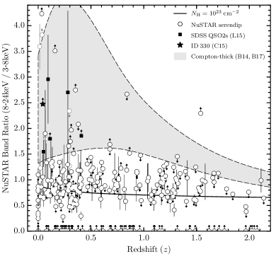
Figure 10.— NuSTAR band ratio ($\mathrm{BR}_{\mathrm{Nu}}$) versus redshift ($z$) for the full NuSTAR serendipitous survey sample (black circles). Sources which are associated with the primary science targets of the NuSTAR observations (according to the $\Delta(cz)$ criterion in Section 2.3) are shown as lighter gray circles. We compare to other NuSTAR-observed sources targetted for other programs (i.e., not part of the serendipitous survey). The black star shows a CT AGN identified in the NuSTAR-COSMOS survey (C15). The black squares show heavily obscured SDSS-selected Type 2 quasars observed with NuSTAR, for which there is evidence for either CT or close to CT absorption (Lansbury et al., 2014; Gandhi et al., 2014; Lansbury et al., 2015). The gray shaded region highlights the parameter space expected for CT (i.e., $N_{\rm H}>1.5\times 10^{24}$ cm^-2) AGNs, considering all populations (including reflection- and transmission-dominated CT AGNs), based on results from the NuSTAR snapshot survey (Baloković et al. 2014; Baloković et al. 2017, in prep.). This gray region was obtained by redshifting the best-fit spectral models of local CT snapshot AGNs, for which the X-ray spectra are relatively well constrained. The upper and lower extents (dashed lines) represent the $68\%$ percentiles (i.e., $84\%$ of the CT snapshot AGNs lie above the lower dashed line). Serendipitous sources lying at $\mathrm{BR}_{\mathrm{Nu}}$ values within or higher than this gray region are good candidates for being CT. The black track shows a MYTorus model prediction for $\mathrm{BR}_{\mathrm{Nu}}$ as a function of redshift, for a more moderate column density of $N_{\rm H}=10^{23}$ cm^-2.

While obscured AGNs can be crudely identified using $\mathrm{BR}_{\mathrm{Nu}}$ alone, an estimate of obscuring columns requires additional knowledge of the source redshifts, which shift key spectral features (e.g., the photoelectric absorption cut-off) across the observed energy bands. Here we use the combination of $\mathrm{BR}_{\mathrm{Nu}}$ and the source redshifts to identify potentially highly obscured objects. Figure 10 shows $\mathrm{BR}_{\mathrm{Nu}}$ versus $z$ for the spectroscopically-identified serendipitous survey sample. We compare with the band ratios measured for CT, or near-CT, SDSS-selected Type 2 quasars observed with NuSTAR in a separate targetted program (Lansbury et al., 2014; Gandhi et al., 2014; Lansbury et al., 2015), and with tracks (gray region) predicted for CT absorption based on redshifting the best-fit spectra of local CT AGNs from the NuSTAR snapshot survey of Swift BAT AGNs (Baloković et al. 2014; Baloković et al. 2017, in prep.). A number of sources stand out as CT-candidates based on this analysis. While $\mathrm{BR}_{\mathrm{Nu}}$ can only provide a crude estimate of the absorbing columns, a more detailed investigation of the NuSTAR spectra and multiwavelength properties of the CT-candidates can strengthen the interpretation of these high-$\mathrm{BR}_{\mathrm{Nu}}$ sources as highly absorbed systems (Lansbury et al., in prep.).

4.1.3 Redshifts and Luminosities

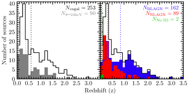
Figure 11.— The distribution of spectroscopic redshifts for the spectroscopically identified NuSTAR serendipitous survey sample. Galactic ($z=0$) sources have been excluded. In addition to the total distribution (black line), the left panel shows the distribution for the subset which are independently detected in the hard band ($8$–$24$ keV; gray filled histogram, left panel) and the right panel shows the distribution separated by optical classification: BLAGNs are shown in blue; NLAGNs are shown in red. The vertical lines mark the median redshifts.

Of the NuSTAR serendipitous survey sources with optical spectroscopic coverage and spectroscopic redshift measurements (described in Section 3.3), there are $262$ identified as extragalactic. Figure 11 shows the redshift distribution for the extragalactic sources, excluding nine sources with evidence for being associated to the NuSTAR targets for their respective observations (see Section 2.3). The redshifts cover a large range, from $z=0.002$ to $3.43$, with a median of $\left<z\right>=0.56$. For the $90$ extragalactic objects with independent detections in the high-energy band ($8$–$24$ keV), to which NuSTAR is uniquely sensitive, the median redshift is $\left<z\right>=0.34$. Roughly comparable numbers of NLAGNs and BLAGNs are identified for lower redshifts ($z\lesssim 1$), but there is a significant bias towards BLAGNs at higher redshifts. This was also found for the NuSTAR surveys in well-studied fields (e.g., C15), and for surveys with sensitive lower energy ($<10$ keV) X-ray observatories such as Chandra and XMM-Newton (e.g., Barger et al. 2003; Eckart et al. 2006; Barcons et al. 2007). This effect is largely due to selection biases against the detection of highly absorbed AGNs, and against the spectroscopic identification of the optically fainter NLAGNs (e.g., Treister et al. 2004).

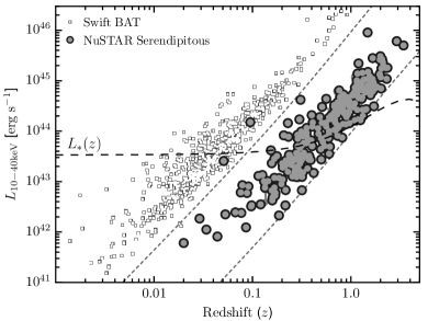
Figure 12.— Rest-frame $10$–$40$ keV luminosity ($L_{\mathrm{10-40\ keV}}$) versus redshift. We compare the NuSTAR serendipitous survey sample (circles) with the Swift BAT 70-month all-sky survey catalog (squares; Baumgartner et al. 2013; blazar and BL Lac types have been excluded). $L_{\mathrm{10-40\ keV}}$ values for the Swift BAT sample are calculated from the $14$–$195$ keV values, assuming $\Gamma_{\rm eff}=2.0$ for the $K$-correction factor (consistent with the median spectral slope for the Swift BAT sources shown). The gray short-dashed lines highlight an observed-frame X-ray flux range spanning two orders of magnitude, from $2\times 10^{-14}$ to $2\times 10^{-12}$ erg s^-1 cm^-2. The black long-dashed line shows the evolution of the knee of the X-ray luminosity function ($L_{*}$) with redshift, as measured by Aird et al. (2015a). The NuSTAR serendipitous survey probes below $L_{*}$ at $z\lesssim 1$.

Figure 12 shows the redshift–luminosity plane for the rest-frame $10$–$40$ keV band. The luminosities are calculated from the observed frame NuSTAR fluxes, assuming an effective photon index of $\Gamma_{\rm eff}=1.8$ (as detailed in Section 2.4). The NuSTAR serendipitous survey covers a large range in $10$–$40$ keV luminosity; the large majority ($99.6\%$; $238/239$) of the unassociated sources lie in the range of $L_{\rm 10-40keV}\approx 10^{42}$ to $10^{46}$ erg s^-1. The median luminosity of $1.2\times 10^{44}$ erg s^-1 is just above the “X-ray quasar” threshold. There is a single outlying source at very low luminosity and redshift, NuSTAR J115851+4243.2 (hereafter J1158; NLAGN; $z=0.0023$; $L_{\rm 10-40keV}=1.0\times 10^{39}$ erg s^-1), hosted by the galaxy IC750. In this case, the SDSS optical spectrum shows a narrow line AGN superimposed over the galaxy spectrum. The source is discussed in detail in a work focusing on the NuSTAR-selected AGNs with dwarf galaxy hosts (Chen et al., submitted). At the other extreme end in luminosity is NuSTAR J052531-4557.8 (hereafter J0525; BLAGN; $z=1.479$; $L_{\rm 10-40keV}=9.0\times 10^{45}$ erg s^-1), also referred to as PKS 0524-460 in the literature. J0525 has an effective NuSTAR photon index of $\Gamma_{\rm eff}=1.9^{+0.3}_{-0.2}$, and a Swift XRT spectrum which is consistent with zero X-ray absorption. The optical spectrum of Stickel et al. (1993) shows a broad line quasar with strong He II, C III], and Mg II emission lines. The source is also radio-bright (e.g., $f_{\rm 1.4GHz}=1.7$ Jy; Tingay et al. 2003) and has been classified as a blazar in the literature (e.g., Massaro et al. 2009).

The most distant source detected is an optically unobscured quasar, NuSTAR J232728+0849.3 (hereafter J2327; BLAGN; $z=3.430$; $L_{\rm 10-40keV}=5.0\times 10^{45}$ erg s^-1), which represents the highest-redshift AGN identified in the NuSTAR survey program to-date. Our Keck optical spectrum for J2327 shows a quasar spectrum with strong Ly$\mathrm{\alpha}$, C IV, and C III] emission lines, and a well-detected Ly$\mathrm{\alpha}$ forest. The source is consistent with having an observed X-ray spectral slope of $\Gamma_{\rm eff}=2$ for both the NuSTAR spectrum and the XMM-Newton counterpart spectrum, and is thus in agreement with being unobscured at X-ray energies. The most distant optically obscured quasar detected is NuSTAR J125657+5644.6 (hereafter J1256; NLAGN; $z=2.073$; $L_{\rm 10-40keV}=2.7\times 10^{45}$ erg s^-1). Our Keck optical spectrum for J1256 reveals strong narrow Ly$\mathrm{\alpha}$, C IV, He II, and C III] emission lines. Analysing the NuSTAR spectrum in combination with a deep archival Chandra spectrum ($\approx 360$ ks of exposure in total), we measure a moderately large line of sight column density of $N_{\rm H}=(1.3\pm 0.4)\times 10^{23}$ cm^-2. This distant quasar is thus obscured in both the optical and X-ray regimes.

In Figure 12 we compare with the 70-month Swift BAT all-sky survey (Baumgartner et al., 2013). The two surveys are highly complementary; the Swift BAT all-sky survey provides a statistical hard X-ray-selected sample of AGNs in the nearby universe (primarily $z<0.1$), while the NuSTAR serendipitous survey provides an equivalent sample (with comparable source statistics) for the distant universe. We compare with the redshift evolution of the knee of the X-ray luminosity function ($L_{\star}$), as determined by Aird et al. (2015a). The Swift BAT all-sky survey samples the population below $L_{\star}$ for redshifts up to $z\approx 0.05$, while the NuSTAR serendipitous survey can achieve this up to $z\approx 1$. There is almost no overlap between the two surveys, which sample different regions of the parameter space. However, there are two NuSTAR sources, outlying in Figure 12, which have very high fluxes approaching the detection threshold of Swift BAT: NuSTAR J043727-4711.5 ($z=0.051$; $L_{\rm 10-40keV}=2.6\times 10^{43}$ erg s^-1) and NuSTAR J075800+3920.4 ($z=0.095$; $L_{\rm 10-40keV}=1.5\times 10^{44}$ erg s^-1). Both are BLAGNs (based on our Keck and NTT spectra), and are unobscured at X-ray energies ($\Gamma_{\rm eff}\approx 1.9$). The former is detected in the 70 month Swift BAT catalog of Baumgartner et al. (2013), and the latter is only detected with Swift BAT at the $\approx 2\sigma$ level, based on the direct examination of the 104 month BAT maps (following the procedures in Koss et al. 2013).

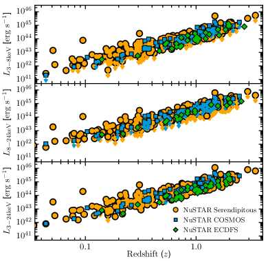
Figure 13.— Luminosity versus redshift for the three NuSTAR energy bands: $3$–$8$ (top), $8$–$24$ (middle), and $3$–$24$ keV (bottom). We compare the NuSTAR serendipitous survey sample (orange circles) with the blank-field NuSTAR surveys of COSMOS (blue squares; C15) and ECDFS (green diamonds; M15).

In Figure 13 we compare the luminosity–redshift source distribution with other NuSTAR extragalactic survey samples: the NuSTAR-ECDFS survey (M15) and the NuSTAR-COSMOS survey (C15). Rest-frame luminosities are shown for the standard three NuSTAR bands ($3$–$8$ keV, $3$–$24$ keV, and $8$–$24$ keV). The serendipitous survey fills out the broadest range of luminosities and redshifts, due to the nature of the coverage (a relatively large total area, but with deep sub-areas that push to faint flux limits).

4.2. Optical properties

4.2.1 The X-ray–optical flux plane

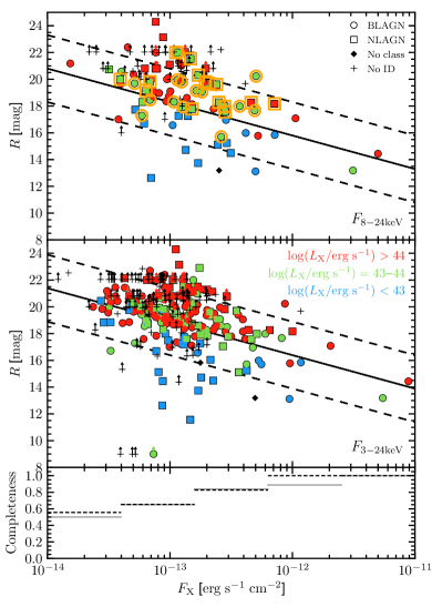
Figure 14.— $R$-band optical magnitude ($R$) versus X-ray flux ($f_{\mathrm{X}}$) for the hard band ($8$–$24$ keV; top panel) and full band ($3$–$24$ keV; middle panel) selected NuSTAR serendipitous survey samples. The blue, green, and red colors highlight three X-ray luminosity ranges, from low to high luminosity, respectively. The solid and dashed lines indicate constant X-ray-to-optical flux ratios of $\log(f_{\rm X}/f_{\rm opt})=0$ and $\pm 1$, respectively. The hard band subsample for which we calculate a reliable Type 2 fraction (see Section 4.2.2) measurement is highlighted with orange outlines. In the bottom panel we show the optical spectroscopic completeness of both the $8$–$24$ (dashed lines) and $3$–$24$ keV (solid lines) samples as a function of $f_{\mathrm{X}}$, calculated as the number of sources with successful optical spectroscopic classifications (see Section 3.3.2) divided by the total number of sources in a given $f_{\mathrm{X}}$ bin.

The X-ray–optical flux plane is a classic diagnostic diagram for sources detected in X-ray surveys (e.g., Maccacaro et al., 1988). This plane has recently been explored for the NuSTAR-COSMOS sample, using the $i$-band (C15). Here we investigate the plane using the optical $R$-band for the NuSTAR serendipitous survey, which provides a relatively large hard X-ray selected sample spanning a comparatively wide flux range. The X-ray-to-$R$-band flux ratio ($f_{\rm X}/f_{\rm opt}$) diagnostic has been widely applied in past Chandra and XMM-Newton surveys of well-known blank fields (e.g., Hornschemeier et al., 2001; Barger et al., 2003; Fiore et al., 2003; Xue et al., 2011). Figure 14 shows the optical $R$-band magnitude ($R$) against X-ray flux ($f_{\mathrm{X}}$) for the NuSTAR serendipitous survey sources which are detected in the hard band ($8$–$24$ keV) and full band ($3$–$24$ keV). We exclude $|b|<10$^∘ and $z=0$ sources, thus minimizing contamination from Galactic sources. We subdivide the NuSTAR sample according to X-ray luminosity and optical spectroscopic classification: objects with successful identifications as either NLAGNs or BLAGNs; objects with redshift constraints, but no classification; and objects with no redshift constraint or classification. For $R>20$, the sources shown with lower limits in $R$ generally correspond to a non-detection in the optical coverage, within the X-ray positional error circle. For sources where it is not possible to obtain an $R$-band constraint (e.g., due to contamination from a nearby bright star), we plot lower limits at the lower end of the y-axis.

We compare with the range of X-ray to optical flux ratios typically observed for AGNs identified in soft X-ray surveys, $-1<\log(f_{\rm X}/f_{\rm opt})<1$ (e.g., Schmidt et al., 1998; Akiyama et al., 2000; Lehmann et al., 2001). To illustrate constant X-ray-to-optical flux ratios, we adopt the relation of McHardy et al. (2003) and correct to the NuSTAR energy bands assuming $\Gamma_{\rm eff}=1.8$. The large majority of sources lie at $\log(f_{\rm X}/f_{\rm opt})>-1$, in agreement with them being AGNs. At least $\approx 25\%$ of the hard-band ($8$–$24$ keV) selected sources lie at $\log(f_{\rm X}/f_{\rm opt})>1$, in agreement with the findings for the lower energy selected X-ray sources detected in the Chandra and XMM-Newton surveys (e.g., Comastri et al., 2002; Fiore et al., 2003; Brandt & Hasinger, 2005). Such high $f_{\rm X}/f_{\rm opt}$ values are interpreted as being driven by a combination of relatively high redshifts and obscuration (e.g., Alexander et al., 2001; Hornschemeier et al., 2001; Del Moro et al., 2008).

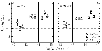
Figure 15.— The X-ray-to-$R$-band flux ratio ($f_{\rm X}/f_{\rm opt}$), as a function of luminosity, for hard band ($8$–$24$ keV) selected sources (left); and full band ($3$–$24$ keV) selected sources (right). The luminosity bins follow those adopted in Figure 14. We show results for the overall spectroscopically identified population (triangles), BLAGN only (circles), and NLAGN only (squares). The solid and dashed horizontal gray lines indicate $\log(f_{\rm X}/f_{\rm opt})=0$ and $\pm 1$, respectively. The horizontal offsets of the data points, within each luminosity bin, are arbitrary and for visualization purposes only.

To demonstrate the dependence on X-ray luminosity and on spectral type, Figure 15 shows median $f_{\rm X}/f_{\rm opt}$ values for bins of X-ray luminosity, and for the NLAGN and BLAGN subsamples separately. The low, medium, and high luminosity bins correspond to $\log(L_{\rm X}/\mathrm{erg\ s^{-1}})<43$, $43<\log(L_{\rm X}/\mathrm{erg\ s^{-1}})<44$, and $\log(L_{\rm X}/\mathrm{erg\ s^{-1}})>44$, respectively. The observed dependence on luminosity and on spectral type is consistent between the hard band and the full band selected samples (left and right panels of Figure 15, respectively). Overall, $f_{\rm X}/f_{\rm opt}$ increases with X-ray luminosity. The increase between the low and medium luminosity bins is highly significant; for the hard-band selected sample, the median $\log(f_{\rm X}/f_{\rm opt})$ value increases from $\approx-0.8$ to $\approx 0.5$. There is a marginally significant overall increase in $f_{\rm X}/f_{\rm opt}$ between the medium and high luminosity bins, which is driven by a significant increase in the $f_{\rm X}/f_{\rm opt}$ values of NLAGNs. A positive correlation between $f_{\rm X}/f_{\rm opt}$ and $L_{\mathrm{X}}$ has previously been identified for Chandra and XMM-Newton samples of optically obscured AGNs selected at $<10$ keV, over the same luminosity range (Fiore et al. 2003). Here we have demonstrated a strong positive correlation for high energy ($\gtrsim 10$ keV) selected AGNs.

In general, the NLAGNs span a wider range in $f_{\rm X}/f_{\rm opt}$ than the BLAGNs, which mostly lie within the range expected for BLAGNs based on soft X-ray surveys, $-1<\log(f_{\rm X}/f_{\rm opt})<1$. The most notable difference between the two classes is in the high-luminosity bin (which represents the “X-ray quasar” regime; $L_{\rm X}>10^{44}$ erg s^-1), where the NLAGNs lie significantly higher than the BLAGNs, with a large fraction at $\log(f_{\rm X}/f_{\rm opt})>1$. This effect can be understood as a consequence of extinction of the nuclear AGN emission. For the BLAGNs the nuclear optical–UV emission contributes strongly to the $R$-band flux, while for the NLAGNs the nuclear optical emission is strongly suppressed by intervening dust (the corresponding absorption by gas at X-ray energies is comparatively weak). The effect is augmented for the high-luminosity bin, where the higher source redshifts ($\left<z\right>\approx 0.9$) result in the observed-frame optical band sampling a more heavily extinguished part of the AGN spectrum, while the observed-frame X-ray band samples a less absorbed part of the spectrum (e.g., Del Moro et al. 2008). The other main difference between the two classes is seen for the lowest luminosity bin where, although the median flux ratios are consistent, the NLAGNs extend to lower values of $f_{\rm X}/f_{\rm opt}$ than the BLAGNs, with a handful of the NLAGNs lying at $\log(f_{\rm X}/f_{\rm opt})<-1$.

4.2.2 The type 2 fraction

Here we investigate the relative numbers of the optically obscured (i.e., NLAGN) and optically unobscured (i.e., BLAGN) populations within the NuSTAR serendipitous survey sample. To provide meaningful constraints on the Type 2 fraction (i.e., the observed number of NLAGNs divided by the total number of NLAGNs+BLAGNs), it is important to understand the sample completeness. We therefore investigate a specific subset of the overall sample for which completeness is well understood: hard band ($8$–$24$ keV) selected sources with $0.1<z<0.5$, $2\times 10^{43}<L_{\rm 10-40\ keV}<2\times 10^{44}$ erg s^-1, and $|b|>10$^∘ (highlighted with orange outlines in the upper panel of Figure 14). The redshift limit ensures that the subsample has high spectroscopic completeness (i.e., the majority of sources have redshifts and classifications from optical spectroscopy; see below), the lower luminosity limit ensures “X-ray completeness” (i.e., the AGN population within this $L_{\mathrm{X}}$–$z$ parameter space has fluxes which lie above the NuSTAR detection limit; e.g., see Figure 12), and the upper luminosity limit is applied to allow comparisons with luminosity-matched comparison samples (see below). The luminosity range samples around the knee of the X-ray luminosity function ($L_{*}$) for these redshifts, $L_{\rm 10-40\ keV}\approx(4$–$7)\times 10^{43}$ erg s^-1 (Aird et al. 2015a). In total, there are $30$ spectroscopically identified sources (all NLAGNs or BLAGNs) within this subsample, which have a median redshift of $\left<z\right>=0.3$. Accounting for sources which are not spectroscopically identified, we estimate an effective spectroscopic completeness of $97$–$100\%$ for this subsample (details are provided in Section A.4).

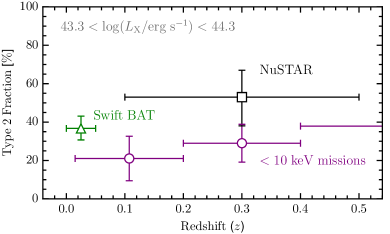
Figure 16.— Observed Type 2 fraction versus redshift for various luminosity-matched ($2\times 10^{43}<L_{\rm X}<2\times 10^{44}$ erg s^-1), X-ray selected AGN samples: the black square shows a hard band ($8$–$24$ keV) selected subset of the NuSTAR serendipitous survey sample with $0.1<z<0.5$; the green triangle shows a subset of the 70-month Swift BAT all-sky survey sample ($z<0.05$; Baumgartner et al. 2013); and the purple circles correspond to a $<10$ keV selected AGN sample, compiled from multiple X-ray surveys (including ASCA, Chandra and XMM-Newton surveys; Hasinger 2008). The horizontal error bars show the redshift limits of each subsample.

The observed Type 2 fraction for the NuSTAR hard band-selected subsample described above is $F_{\rm Type\ 2}=53^{+14}_{-15}\%$ (binomial uncertainties). If we instead use the sources selected in the full band ($3$–$24$ keV), a similar fraction is obtained ($F_{\rm Type\ 2}=48\pm 11\%$). In Figure 16 we compare with the Type 2 fraction for nearby ($z<0.05$) AGNs similarly selected at high X-ray energies ($>10$ keV). To obtain this data point we calculate the observed Type 2 fraction for the 70-month Swift BAT all-sky survey. Importantly, we use a luminosity-matched subsample of the Swift BAT survey ($2\times 10^{43}<L_{\rm 10-40\ keV}<2\times 10^{44}$ erg s^-1, as for the NuSTAR subsample), since the Type 2 fraction likely varies with luminosity. We apply a redshift cut of $z<0.05$ to ensure X-ray completeness (redshifts above this threshold push below the flux limit of Swift BAT for the adopted $L_{\rm 10-40\ keV}$ range; see Figure 12). For consistency with our approach for the NuSTAR sample, we class Swift BAT AGNs with intermediate types of $1.9$ or below as BLAGNs, those with NL Sy1 type spectra as BLAGNs, and those with galaxy type optical spectra as NLAGNs. The observed Type 2 fraction for this luminosity-matched Swift BAT sample at $z<0.05$ is $F_{\rm Type\ 2}=37\pm 6\%$, slightly lower than our NuSTAR-measured Type 2 fraction at $z\approx 0.3$, but consistent within the uncertainties. A caveat to this comparison is that the spectroscopic completeness of the Swift BAT subsample is unknown; overall there are $\approx 100$ sources in the Baumgartner et al. (2013) catalog which are consistent with being AGNs but lack an optical spectroscopic redshift and classification, some of which could potentially lie within the luminosity and redshift ranges adopted above. Making the extreme assumption that these $\approx 100$ sources all lie in the above luminosity and redshift ranges, and are all NLAGNs, the maximum possible Swift BAT $F_{\rm Type\ 2}$ value is $66\%$ (which would still be in agreement with the NuSTAR-measured fraction). Depending on the full duration of the NuSTAR mission, the source numbers for the NuSTAR serendipitous survey may feasibly increase by a factor of two or more, which will reduce the uncertainties on the Type 2 fraction. However, to determine reliably whether there is evolution in the Type 2 fraction of high energy selected AGNs between $z<0.05$ and $z>0.1$, future studies should systematically apply the same optical spectroscopic classification methodologies to both samples. An early indication that the obscured fraction of AGN might increase with redshift was given by La Franca et al. (2005), and this has been further quantified in subsequent works (e.g., Ballantyne et al., 2006; Treister & Urry, 2006; Hasinger, 2008; Merloni et al., 2014). The slope of the increase with redshift is consistent with that found by Treister & Urry (2006).

The Type 2 fraction has been thoroughly investigated for the AGN population selected by lower energy ($<10$ keV) X-ray missions such as Chandra and XMM-Newton. Hasinger (2008) presented a relatively complete $2$–$10$ keV selected sample, compiled from a variety of surveys with $<10$ keV missions (also see Merloni et al. 2014 for a more recent study of XMM-Newton-selected sources at $0.3<z<3.5$). We consider the $0.2<z<0.4$ subset of the Hasinger (2008) sample, in order to match to our NuSTAR subsample in redshift as closely as possible, and we limit to the luminosity range explored above ($2\times 10^{43}<L_{\rm 10-40\ keV}<2\times 10^{44}$ erg s^-1; we assume a luminosity band correction of $L_{\rm 10-40\ keV}/L_{\rm 2-10\ keV}=1$). The Type 2 fraction for this subset of the Hasinger (2008) sample is $F_{\rm Type\ 2}=29\pm 10\%$, which is lower than our NuSTAR-measured Type 2 fraction (see Figure 16), but only at a significance level of $\approx 2\sigma$. This could be explained as a result of the different selection functions of different X-ray missions, with the high energy ($>8$ keV) selection of NuSTAR being less biased against obscured sources. Another factor to consider is the different classification methodologies applied. In addition to optical spectroscopic constraints, Hasinger (2008) use additional X-ray hardness information to classify ambiguous sources as NLAGNs or BLAGNs. Hasinger (2008) do assess the extent to which the Type 2 fraction measurements change if, instead, only the pure optical spectroscopic classification is adopted (i.e., a similar approach to our spectroscopic classification for the NuSTAR sources) and find that, for the redshift and luminosity ranges explored here, the Type 2 fraction would be somewhat higher but unlikely to increase by more than a factor of $\approx 1.2$.

In Figure 16 we compare with additional luminosity-matched subsamples for the adjacent redshift bins studied by Hasinger (2008). The high-energy selected AGN samples (NuSTAR and Swift BAT) appear to lie systematically higher in Type 2 fraction than the luminosity-matched lower energy ($<10$ keV) selected AGNs, for the redshift ranges covered. We note that the Type 2 fraction constraints of Merloni et al. (2014) for $<10$ keV selected AGNs are broadly consistent with the values shown in Figure 16 (we primarily compare with the Hasinger 2008 sample since the source redshifts and luminosities sampled facilitate a direct comparison of results). The apparently small numbers of CT AGNs identified (e.g., see Figure 10) suggest that the offset in Type 2 fraction is not primarily driven by the uncovering of a new CT population, but more likely by the selection functions of NuSTAR and Swift BAT being generally less biased against significantly obscured AGNs.

4.3. Infrared properties

4.3.1 WISE colors

Mid-infrared (MIR; $\gtrsim 5$ µm) emission from AGNs is primary emission that has been reprocessed by circumnuclear dust, and suffers little extinction relative to other (e.g., optical and soft X-ray) wavelengths. Color selections using the WISE telescope bands (e.g., Assef et al., 2010; Jarrett et al., 2011; Stern et al., 2012; Mateos et al., 2012, 2013; Assef et al., 2013) can separate bright AGNs from host-galaxy light (from stars and the interstellar medium) through the identification of a red MIR spectral slope, and have thus become widely applied. These selections have the potential to identify large samples of AGNs with less bias against heavily obscured systems. However, their effectiveness worsens toward lower AGN luminosities, where identifying the AGN component of the MIR spectrum is more problematic. Here we investigate the MIR properties of our NuSTAR serendipitous survey sample, and consider the results with respect to these AGN selection criteria.

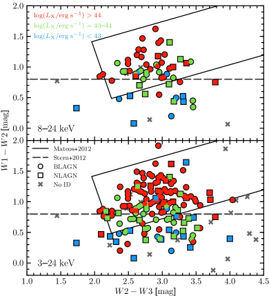
Figure 17.— WISE color–color diagram of NuSTAR serendipitous survey AGNs as a function of X-ray luminosity ($L_{\mathrm{X}}$) and source classification, for hard-band ($8$–$24$ keV) selected sources (top) and full-band ($3$–$24$ keV) selected sources (bottom). BLAGN and NLAGN are shown as circles and squares, respectively, while sources without a spectroscopic identification are shown as gray crosses. The blue, green, and red colors highlight three X-ray luminosity ranges, from low to high luminosity, respectively. The luminosities correspond to the selection bands used for this analysis (i.e., $L_{\mathrm{8-24\ keV}}$ and $L_{\mathrm{3-24\ keV}}$ for the upper and lower panels, respectively). We compare with the AGN ‘wedge’ of Mateos et al. (2012) and the AGN color cut of Stern et al. (2012; $W{\rm 1}$–$W{\rm 2}\geq 0.8$).

Figure 17 shows a WISE color–color diagram ($W{\rm 1}$–$W{\rm 2}$ versus $W{\rm 2}$–$W{\rm 3}$) for the NuSTAR serendipitous survey subsamples which are selected (i.e., independently detected) in the hard band ($8$–$24$ keV; upper panel) and full band ($3$–$24$ keV; lower panel). In general, the sources which lie at higher (i.e., redder) $W{\rm 1}$–$W{\rm 2}$ values have stronger AGN contributions to their MIR SEDs. We exclude low Galactic latitude sources ($|b|<10$^∘), and sources which are spectroscopically confirmed as Galactic. In addition, we only consider sources with well constrained X-ray positions (i.e., with Chandra, Swift XRT, or XMM-Newton positions), and we limit the analysis to the fraction of these sources ($70\%$ and $61\%$ for the hard and full band, respectively) with significant detections in all three of the relevant, shorter wavelength WISE bands ($W{\rm 1}$, $W{\rm 2}$, and $W{\rm 3}$; which are centered at $3.4$ µm, $4.6$ µm, and $12$ µm, respectively). Figure 17 shows the sample subdivided according to X-ray luminosity and optical spectral classification. In Figure 18 we show the fraction ($f_{\mathrm{wedge}}$ hereafter) of sources which are selected as AGNs based on MIR colors alone, according to the selection “wedge” of Mateos et al. (2012), as a function of X-ray luminosity and optical classification.

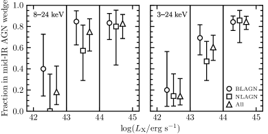
Figure 18.— The fraction of extragalactic NuSTAR serendipitous survey sources which are selected as AGNs based on MIR colors alone (i.e., they lie in the WISE color wedge of Mateos et al. 2012), as a function of luminosity, for hard-band ($8$–$24$ keV) selected sources (left) and full-band ($3$–$24$ keV) selected sources (right). The luminosity bins follow those adopted in Figure 17. We show results for the overall spectroscopically identified population (triangles), BLAGN only (circles), and NLAGN only (squares). The error bars show binomial uncertainties. The horizontal offsets of the data points, within each luminosity bin, are arbitrary and for visualization purposes only.

For the NuSTAR AGNs selected in the full band (lower panel of Figure 17 and right panel of Figure 18) the overall fraction of sources identified as AGNs in the MIR is $f_{\rm wedge}=64.9^{+5.7}_{-6.2}\%$ ($111/171$). Considering sources with optical spectroscopic classifications, the fractions for the overall BLAGN and NLAGN samples are $f_{\rm wedge}=77.6^{+5.9}_{-7.2}\%$ ($83/107$) and $48.9^{+11.9}_{-11.8}\%$ ($22/45$), respectively. NLAGNs are therefore significantly less likely to be identified as AGNs based on MIR colors alone. This is largely driven by the lower luminosity, on average, of the NLAGNs (median of $4\times 10^{43}$ erg s^-1) compared to the BLAGNs (median of $3\times 10^{44}$ erg s^-1), in combination with the fact that $f_{\mathrm{wedge}}$ decreases toward lower luminosities (see Figure 18). Matching the NLAGNs and BLAGNs in luminosity, we do not find statistically significant differences in $f_{\rm wedge}$ between the two classes.

For the remainder of our overall sample which lack optical spectroscopic classifications (gray crosses in Figure 17), the WISE colors are informative of their likely properties. A low fraction of these sources lie within the wedge, $f_{\rm wedge}=27.8^{+19.3}_{-13.5}$ ($5/18$). This suggests that, statistically, the unidentified sources are likely to be less luminous AGNs. In combination with the poor success rate for optical spectroscopy of these sources, we expect that they are likely to be dominated by optically obscured, low luminosity systems.

The results in Figure 18 show that MIR selections miss a significant fraction of the NuSTAR-selected AGN population, with the missed fraction increasing from $\approx 15\%$ at high luminosities, to $\approx 80\%$ at the lower luminosity end. The dependence of MIR selections on AGN luminosity has been identified for lower energy X-ray selected AGN samples (e.g., Cardamone et al. 2008; Eckart et al. 2010), and is likely primarily driven by a stronger contribution to the SED from the host galaxy for lower X-ray luminosities, which results in bluer MIR colors. The MIR AGN selection wedge of Mateos et al. (2012) was defined using the Bright Ultrahard XMM-Newton survey (BUXS) sample, selected at $4.5$–$10$ keV, for comparable numbers of spectroscopically identified AGNs ($114$ BLAGNs and $81$ NLAGNs) as the full-band selected NuSTAR serendipitous survey sources incorporated here ($107$ BLAGNs and $45$ NLAGNs), and for a similar redshift and luminosity distribution. For the NLAGNs, our results for $f_{\rm wedge}$ as a function of X-ray luminosity and optical classification are consistent (given the uncertainties) with those found for the BUXS sample. Our BLAGNs have marginally lower $f_{\rm wedge}$ values than the BUXS BLAGNs. For instance, Mateos et al. (2012) find that the MIR selection is essentially complete for BLAGNs at $L_{\rm X}>10^{43}$ erg s^-1 (e.g., $f_{\rm wedge}=100_{-6.6}\%$ and $96.1^{+3.0}_{-6.3}\%$ for $L_{\rm 2-10keV}=10^{43}$–$10^{44}$ and $10^{44}$–$10^{45}$ erg s^-1, respectively), while even at the highest luminosities ($L_{\rm 3-24keV}>10^{44}$ erg s^-1) we find $f_{\rm wedge}=84.2^{+5.7}_{-8.0}\%$.

It is notable that the MIR selection fails for $12$ (i.e., $15.8\%$) of the high luminosity NuSTAR-selected BLAGNs, since MIR selections are typically expected to be close to complete for high luminosity, unobscured sources. To assess why these sources in particular are not MIR-selected, we compare their source properties (e.g., NuSTAR detection significance, redshift, $10$–$40$ keV luminosity, $2$–$10$ keV luminosity, brightness, optical spectra, Galactic latitude) with the $64$ (i.e., the $84.2\%$) high luminosity BLAGNs which are MIR-selected. There are no clear statistically significant differences, with a possible exception: the optical $R$-band magnitude distributions of the two subsets are different at a moderate significance level (KS-test p-value of $p=0.037$), with the $12$ MIR-unselected sources skewed to fainter $R$ values (median of $\left<R\right>=19.9$) than their MIR-selected counterparts ($\left<R\right>=19.4$). This result increases in significance (to $p=0.0075$) if we limit the comparison to the eight (out of $12$) MIR-unselected sources which are additionally missed by the Stern et al. (2012) $W{\rm 1}$–$W{\rm 2}$ color AGN selection. Comparing the distribution of $f_{\rm X}/f_{\rm opt}$ versus $W{\rm 1}$–$W{\rm 2}$ for these eight sources with the overall serendipitous sample (see Figure 19), they overlap with lower luminosity AGNs where we expect that the relatively blue $W{\rm 1}$–$W{\rm 2}$ colors are driven by a stronger (relative) contribution to the MIR SED from the host galaxy.

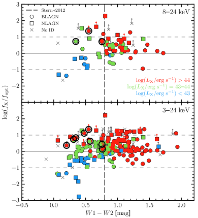
Figure 19.— The X-ray-to-$R$-band flux ratio ($f_{\rm X}/f_{\rm opt}$) versus the WISE $W{\rm 1}$–$W{\rm 2}$ color, for hard band ($8$–$24$ keV) selected sources (top); and full band ($3$–$24$ keV) selected sources (bottom). The luminosity bins and the marker labelling follow those adopted in Figures 14 and 17. Eight high luminosity BLAGNs which are not selected as AGNs in the MIR (see Section 4.3.1) are highlighted with large black circles.

The latter could also be true for the eight MIR-unselected high-$L_{\mathrm{X}}$ BLAGNs if their MIR AGN luminosities are relatively low compared to the $64$ MIR-selected counterparts (which are matched in X-ray luminosity). Estimating the rest-frame $6$ $\mu$m luminosities ($L_{\rm 6\mu m}$) by interpolating between the relevant observed-frame WISE band magnitudes, we find that the eight MIR-unselected BLAGNs have a different $L_{\rm 6\mu m}$ distribution to the MIR-selected counterparts ($p=0.046$), and are indeed skewed to lower MIR luminosities ($\left<L_{\rm 6\mu m}\right>=3.4\times 10^{44}$ erg s^-1) than the MIR-selected sources ($\left<L_{\rm 6\mu m}\right>=1.3\times 10^{45}$ erg s^-1). In summary, the incompleteness of MIR selections for unobscured high-$L_{\mathrm{X}}$ AGNs appears to be related to scatter in the intrinsic AGN properties. The luminous MIR-unselected sources could potentially represent AGNs which are lacking in hot dust emission (i.e., “hot-dust-poor” AGNs; e.g., Hao et al. 2010), although the inferred hot-dust-poor fraction ($\sim 10$–$15\%$) would be unexpectedly high compared to that observed for optically selected quasars ($\sim 1\%$; Jun & Im 2013).

For the NuSTAR serendipitous survey sources selected in the hard band (upper panel of Figure 17 and left panel of Figure 18), for which NuSTAR is uniquely sensitive, the results are consistent with those for the full-band sample, but with greater uncertainties due to the smaller source numbers. For instance, $f_{\rm wedge}=67.6^{+8.5}_{-9.8}\%$ ($46/68$) for the overall hard band selected sample. We conclude that, while there are some small differences, the MIR color distribution of the NuSTAR serendipitous survey sample is largely consistent with that expected based on the results for lower-energy ($<10$ keV) selected AGNs.

4.3.2 X-ray–MIR luminosity plane

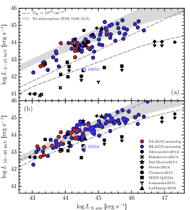
Figure 20.— Observed (i.e., uncorrected for absorption) rest-frame $2$–$10$ keV [$L_{\mathrm{2-10\ keV}}$; (a)] and $10$–$40$ keV X-ray luminosity [$L_{\mathrm{10-40\ keV}}$; (b)] versus rest-frame $6$ $\mu$m luminosity ($L_{\rm 6\mu m}$, in $\mathrm{\nu}L_{\mathrm{\nu}}$ units). Filled circles show the NuSTAR serendipitous survey sources. We only show sources that have detections in the WISE bands necessary to estimate $L_{\rm 6\mu m}$ (through interpolation), and which are AGN-dominated at MIR wavelengths according to their WISE colors (based on satisfying either the Mateos et al. 2012 or Stern et al. 2012 criteria), and thus where we believe $L_{\rm 6\mu m}$ to have minimal contamination from the host galaxy. The apparently X-ray weak source J0650 (see Sections 4.3.2 and A.5) is shown as an empty circle and labelled. We compare with other samples: NuSTAR-observed SDSS-selected heavily obscured Type 2 quasars (squares; $z=0.05$–$0.49$; Lansbury et al. 2014; Gandhi et al. 2014; Lansbury et al. 2015); three CT Seyfert 2 AGNs from the NuSTAR snapshot survey (“$\times$” symbols; $z\approx 0.01$; Baloković et al. 2014); luminous and heavily obscured WISE-selected AGNs targetted with NuSTAR (diamonds; $z\approx 2$; Stern et al., 2014); a heavily obscured quasar identified in the NuSTAR-ECDFS survey (star; $z\approx 2$; Del Moro et al., 2014); a CT AGN identified in the NuSTAR-COSMOS survey (pentagon; ID 330; $z=0.044$; C15); a candidate heavily CT AGN identified in the COSMOS field (triangle; $z=0.35$; Lanzuisi et al. 2015); and NuSTAR-observed FIRST-2MASS red quasars (triangle; $z=0.14$–$0.41$; LaMassa et al. 2016). All of the data are compared with the luminosity ratios expected in the case of zero line-of-sight absorption (gray region). This region shows the range of intrinsic luminosity ratios predicted by three different intrinsic relations in the literature: Gandhi et al. (2009), Fiore et al. (2009) and Stern (2015). The dashed lines illustrate the observed X-ray luminosity suppression expected if the zero absorption region is absorbed by gas with a column density of $N_{\rm H}=10^{24}$ cm^-2.

There is a remarkably tight correlation between the X-ray luminosities and the MIR luminosities of unobscured AGNs, with both providing estimates of the intrinsic AGN power (e.g., Lutz et al., 2004; Fiore et al., 2009; Gandhi et al., 2009; Lanzuisi et al., 2009; Ichikawa et al., 2012; Matsuta et al., 2012; Asmus et al., 2015; Mateos et al., 2015; Stern, 2015). Low X-ray to MIR luminosity ratios are interpreted as being due to either X-ray absorption or intrinsic X-ray weakness.

In Figure 20 we show the observed (i.e., uncorrected for absorption) rest-frame X-ray luminosities ($L_{\rm X}^{\rm obs}$) versus the rest-frame $6$ $\mu$m luminosities ($L_{\rm 6\mu m}$, in $\nu L_{\nu}$ units) for NuSTAR serendipitous survey sources. We only include sources which are AGN-dominated at MIR wavelengths according to the WISE colors (based on either of the criteria in Section 4.3.1), and thus where we believe the rest-frame $6$ $\mu$m flux to be dominated by the AGN rather than host-galaxy light. Additionally, we require the sources to be detected in the two observed-frame WISE bands which are interpolated between to estimate $L_{\rm 6\mu m}$ (e.g., $W{\rm 2}$ and $W{\rm 3}$ for $z<1$). For the high energy ($10$–$40$ keV) rest-frame X-ray band (bottom panel of Figure 20), the X-ray luminosities are from NuSTAR photometry (as described in Section 2.4). For the low energy ($2$–$10$ keV) rest-frame X-ray band (top panel of Figure 20), the X-ray luminosities are estimated from CSC or 3XMM counterpart fluxes (for the top panel, we only show sources with counterparts in these catalogs). We compare with other NuSTAR-observed samples, including a number of heavily obscured AGNs. To demonstrate the approximate X-ray to MIR luminosity ratios expected in the cases of zero absorption and high absorption, we show the intrinsic X-ray–MIR relation (as measured by multiple studies; Fiore et al. 2009; Gandhi et al. 2009; Stern 2015) and the same relation after absorption by $N_{\rm H}=10^{24}$ cm^-2 gas, respectively.

At $10$–$40$ keV, the serendipitous survey sources are generally consistent with both the intrinsic and the highly absorbed X-ray–MIR relations (which are close together for these energies). The most outlying source, J0650 (highlighted in Figure 20), has a very low upper limit in X-ray to MIR luminosity ratio. Notably, for this source the Keck optical spectroscopy reveals a narrow line Seyfert 1 (NL Sy1) spectrum, and we measure a very steep $0.5$–$10$ keV X-ray spectrum ($\Gamma_{\rm eff}=3.1$). Given these properties, we interpret the low X-ray to MIR ratio as likely being driven by intrinsic X-ray weakness (in combination with the steep X-ray spectrum), rather than being driven by extreme absorption levels. Intrinsic X-ray weakness has previously been identified for objects in the NL Sy1 class (e.g., Miniutti et al. 2012; Leighly et al. 2007b, a). A detailed discussion of J0650 is provided in Section A.5.

At $2$–$10$ keV, the sample shows evidence for significant downwards deviations from the intrinsic relations, although there is little overlap with the known heavily absorbed and CT sources which have been observed in targetted NuSTAR programs. We note however that this analysis is currently limited to a specific subset of the serendipitous survey (i.e., sources which are AGN-dominated at MIR wavelengths, and which are detected in the relevant WISE bands). Future SED modelling of the broader spectroscopically identified sample would allow reliable $L_{\rm 6\mu m}$ measurements (disentangling AGN and host galaxy MIR emission) for a more complete subset of the serendipitous survey sample.

5. Summary

The high sensitivity of NuSTAR at $\gtrsim 10$ keV has provided access to large samples of high-energy X-ray emitting AGNs in the distant universe, whereas previous observatories were largely restricted to the local universe ($z\lesssim 0.1$). In this paper we have presented the first full catalog for the NuSTAR serendipitous survey, the largest survey undertaken with NuSTAR, which incorporates data from the first 40 months of telescope operation. The data include $331$ unique fields, with a total areal coverage of $13\ \mathrm{deg}^{2}$, and a cumulative exposure time of $\approx 20$ Ms. We have characterized the NuSTAR detected AGNs in terms of their X-ray, optical, and IR properties. Below we summarize the main results:

• Overall, we detect $497$ sources which are significant post-deblending (i.e., after accounting for contamination of the photon counts from nearby sources). Of these, $163$ are independently detected in the hard ($8$–$24$ keV) energy band; see Section 2.5.

• The median vignetting-corrected exposure time per source (for the combined FPMA+FPMB data) is $\left<t_{\rm net}\right>=60$ ks, and the maximum is $1500$ ks. The X-ray fluxes span from $f_{\rm 3-24keV}\approx 10^{-14}$ to $10^{-11}$ erg s^-1 cm^-2, with a median value of $\left<f_{\rm 3-24keV}\right>=1.1\times 10^{-13}$ erg s^-1 cm^-2; see Section 4.1.1. The survey reaches flux depths similar to the NuSTAR surveys in well-studied fields (COSMOS, ECDFS, EGS, GOODS-N, and UDS) over comparable areas (see Section 2.3), and is $\approx$two orders of magnitude fainter than the Swift BAT surveys; e.g., see Section 4.1.3.

• There is a large range in the observed band ratios of AGNs at $3$–$24$ keV, which imply a range of effective photon indices going from very soft ($\Gamma_{\rm eff}\approx 3$) to very hard ($\Gamma_{\rm eff}\approx 0$); see Section 4.1.2. We find no evidence for an anticorrelation between band ratio and count rate, as has previously been found for lower energy X-ray bands; see Section 4.1.2.

• A large fraction $79\%$ ($395/497$) of the sources have soft ($<10$ keV) X-ray counterparts detected in surveys or archival data from XMM-Newton, Chandra, and Swift XRT. The NuSTAR fluxes and the soft X-ray counterpart fluxes show good agreement for the $3$–$8$ keV energy band, and the maximum identified variation in AGN flux between the soft X-ray and NuSTAR observations is a factor of $\approx$five; see Section 3.1. The higher positional accuracies of the soft X-ray observatories relative to NuSTAR allow us to reliably match to optical and IR counterparts; see Section 3.2.

• Optical spectroscopic identifications (i.e., redshift measurements and source classifications) have been successfully obtained for $276$ sources. For the large majority of the sample ($222$ sources) this was achieved through our extensive campaign of ground-based spectroscopic followup, using a range of observatories at multiple geographic latitudes; see Section 3.3. $16$ sources are spectroscopically confirmed as Galactic. Of the $260$ extragalactic sources (AGNs), $162$ ($62.3\%$) are classified as BLAGNs, $97$ ($37.3\%$) are NLAGNs, and one ($0.4\%$) is a BL Lac; see Section 3.3.2. While similar numbers of NLAGNs and BLAGNs are identified at lower redshifts ($z\lesssim 1$) there is a bias towards detections of BLAGNs at higher redshifts; this bias has been well established for other X-ray missions (e.g., Chandra and XMM-Newton); see Section 4.1.3.

• The serendipitous survey AGNs have redshifts covering a wide range, from $z=0.002$ to $3.4$, with a median of $\left<z\right>=0.56$. The rest-frame $10$–$40$ keV luminosities also span a wide range, from $L_{\rm 10-40keV}\approx 10^{39}$ to $10^{46}$ erg s^-1, with a median value of $\left<L_{\rm 10-40keV}\right>=10^{44.1}$ erg s^-1. Previous X-ray missions with sensitivity at $>10$ keV were able to sample the AGN population below the knee of the X-ray luminosity function ($L_{\star}$) for redshifts up to $z\approx 0.05$, and NuSTAR extends this to $z\approx 1$; see Section 4.1.3.

• We present the X-ray–optical flux plane for the optical $R$ band, and the $8$–$24$ keV and $3$–$24$ keV NuSTAR bands. The majority of sources have $f_{\rm X}/f_{\rm opt}$ values consistent with those expected for AGNs based on the findings of previous low energy ($<10$ keV) X-ray observatories. We find a strong, positive correlation between $f_{\rm X}/f_{\rm opt}$ and X-ray luminosity, in agreement with results at $<10$ keV. We also find evidence for significant differences in $f_{\rm X}/f_{\rm opt}$ between the BLAGNs and NLAGNs; see Section 4.2.1.

• We measure a Type 2 AGN fraction of $53^{+14}_{-15}\%$ for an effectively spectroscopically complete subset of the hard band ($8$–$24$ keV) selected sample at $0.1<z<0.5$ and with $2\times 10^{43}<L_{\rm 10-40keV}<2\times 10^{44}$ erg s^-1. Comparing with luminosity-matched $z<0.05$ AGNs selected by the Swift BAT survey, the NuSTAR-measured Type 2 fraction for distant AGNs is higher, but consistent within the uncertainties. However, the NuSTAR-measured and Swift BAT-measured Type 2 fractions appear to be systematically higher than those measured for redshift- and luminosity-matched AGNs selected by $<10$ keV X-ray missions (e.g., Chandra and XMM-Newton); see Section 4.2.2.

• We compare the distribution of WISE $W{\rm 1}$–$W{\rm 2}$ and $W{\rm 2}$–$W{\rm 3}$ colors for NuSTAR AGNs with commonly applied MIR color-selection techniques. The fraction of NuSTAR AGNs which would be selected as AGNs based on the MIR colors alone is a strong function of X-ray luminosity, in agreement with findings for low energy ($<10$ keV) X-ray selected samples. The fraction of NuSTAR AGNs missed by MIR color-selections is large, ranging between $\approx 15\%$ and $\approx 80\%$ for the highest luminosities ($L_{\rm X}>10^{44}$ erg s^-1) and the lowest luminosities ($L_{\rm X}<10^{43}$ erg s^-1), respectively; see Section 4.3.1. It is notable that a number of luminous NuSTAR-selected BLAGNs are not selected in the MIR, and that this appears to be driven by the intrinsic AGN properties; see Section 4.3.1.

• We present the X-ray–MIR luminosity plane for sources which are AGN-dominated at MIR wavelengths. For both the rest-frame $2$–$10$ keV and $10$–$40$ keV bands the large majority of the sources are consistent with being scattered around the intrinsic $L_{\rm X}$–$L_{\rm 6\mu m}$ relation; see Section 4.3.2. One source is highlighted as having an extremely low $L_{\rm 10-40keV}/L_{\rm 6\mu m}$ ratio (J0650; $z=0.32$; $L_{\rm 6\mu m}\approx 4\times 10^{44}$ erg s^-1; $L_{\rm 10-40keV}<2\times 10^{43}$ erg s^-1). A detailed investigation reveals a narrow-line Seyfert 1, likely to be intrinsically X-ray weak as opposed to heavily obscured; see Section 4.3.2.

The NuSTAR serendipitous survey presented herein is the largest sample of distant AGNs selected with a focusing high energy ($\gtrsim 10$ keV) X-ray observatory. As the NuSTAR science operations continue into the future, the serendipitous survey will continue to grow at a similar rate, and is likely to eventually achieve a sample size on the order of $\gtrsim 1000$ sources. This will result in improved statistical constraints on the overall properties of the hard X-ray emitting source population, and will facilitate the discovery of rare and extreme sources not sampled as effectively by the smaller-area dedicated NuSTAR surveys (e.g., in the COSMOS, ECDFS, EGS, GOODS-N, and UDS fields). A continued program of followup observations will be necessary to maximize the effectiveness of the serendipitous survey.

Appendix A A.1. Description of the NuSTAR Serendipitous Survey Source Catalog

The NuSTAR serendipitous survey source catalog, containing $498$ sources in total, is available as an electronic table. Here we describe the columns of the catalog, which are summarized in Table 5.

Table 5Column Descriptions for the Primary NuSTAR Serendipitous Source Catalog

Column number	Description
1	Unique source identification number (ID).
2	Unique NuSTAR source name.
3, 4	Right ascension (R.A.) and declination (decl.).
5–7	Flags indicating the energy bands for which the source is detected.
8–10	Same as columns 5–7, post-deblending.
11–13	Logarithm of the false probabilities for the three standard energy bands.
14–16	Same as columns 11–13, post-deblending.
17	Flag indicating whether the source is significant post-deblending, for at least one energy band.
18–32	Total, background, and net source counts for the three standard energy bands, and associated errors.
33–44	Same as columns 18–32, post-deblending.
45–47	Net vignetting-corrected exposure times at the source position, for the combined A+B data.
48–62	Total, background, and net source count rates for the three standard energy bands, and associated errors.
63–68	Deblended net source count rates for the three standard energy bands, and associated errors.
69–71	Band ratio and upper and lower errors.
72–74	Effective photon index and upper and lower errors.
75–80	Deblended fluxes in the three standard bands and associated errors.
81	Reference for the adopted lower-energy X-ray (Chandra, XMM-Newton or Swift XRT) counterpart.
82, 83	R.A. and decl. of the lower-energy X-ray counterpart.
84	Angular separation between the NuSTAR and lower-energy X-ray counterpart positions.
85	$3$–$8$ keV (3XMM or CSC) flux of the lower-energy X-ray counterpart.
86	Total $3$–$8$ keV flux of all (3XMM or CSC) sources within $30\arcsec$ of the NuSTAR position.
87, 88	R.A. and decl. of the adopted WISE counterpart.
89	Angular separation between the NuSTAR and WISE counterpart positions.
90–97	WISE magnitudes in the four standard bands and associated errors.
98	Reference for the adopted optical counterpart.
99, 100	R.A. and decl. of the optical counterpart.
101	Angular separation between the NuSTAR and optical counterpart positions.
102	$R$-band magnitude for the optical counterpart.
103	Spectroscopic redshift.
104	Non-absorption-corrected, rest-frame $10$–$40$ keV luminosity.
105	Binary flag to indicate sources associated with the primary science targets of their respective NuSTAR fields.
106	Binary flag to indicate the sources used for the Aird et al. (2015b) study.

Notes. The full catalog is available as a machine readable electronic table.

Column 1: the unique source identification numbers (ID), in order of increasing right ascension (R.A.).

Column 2: the unique NuSTAR source names, following the IAU-approved format: NuSTAR JHHMMSS$\pm$DDMM.m, where m is the truncated fraction of one arcminute for the arcseconds component of the declination (decl.).

Columns 3, 4: the NuSTAR R.A. and decl. coordinates (J2000), as described in Section 2.3.

Columns 5–7: a binary flag indicating whether the source is detected with a false probability lower than our threshold of $\log(P_{\rm False})=-6$, for the soft ($3$–$8$ keV), hard ($8$–$24$ keV), and full ($3$–$24$ keV) bands. These three bands are abbreviated as SB, HB, and FB, respectively, throughout the source catalog.

Columns 8–10: the same as columns 5–7, after deblending has been performed to account for contamination of the source counts from very nearby sources (see Section 2.4 of this paper, and Section 2.3.2 of M15. Deblending only affects a very small fraction of the overall sample (e.g., see Section 2.4).

Columns 11–13: the logarithm of the false probabilities ($P_{\rm False}$) of the NuSTAR detected sources, for the three standard energy bands (see Section 2.3).

Columns 14–16: the same as columns 11–13, after deblending has been performed.

Column 17: a binary flag indicating whether the NuSTAR detected source remains significant after deblending, in at least one of the three standard energy bands.

Columns 18–32: photometric quantities, calculated at the source coordinates in columns 3 and 4, and using a source aperture of $30^{\prime\prime}$ radius (see Section 2.4). The values are non-aperture-corrected; i.e., they correspond to the $30^{\prime\prime}$ values, and have not been corrected to the full PSF values. We provide the total counts (i.e., all counts within the source aperture) and associated errors ($84\%$ CL), the background counts scaled to the source aperture, and the net source counts (i.e., total minus background) and associated errors. For the net source counts, we give $90\%$ CL upper limits for sources not detected in a given band. Throughout the table, upper limits are flagged with a $-99$ value in the error column.

Columns 33–44: the same as columns 18–32, after deblending has been performed.

Columns 45–47: the average net, vignetting-corrected exposure time at the source coordinates (columns 3 and 4), for each energy band. These correspond to the A+B data, so should be divided by two to obtain the average exposure per FPM. Units: $\mathrm{s}$.

Columns 48–62: the non-aperture-corrected total, background, and net count rates (and associated errors; $84\%$ CL) determined from the photometric values in columns 18–32, and the exposure times in columns 45–47. Units: $\mathrm{s^{-1}}$.

Columns 63–68: the deblended net count rates, and associated errors, determined from the photometric values in columns 33–44, and the exposure times in columns 45–47. Units: $\mathrm{s^{-1}}$.

Columns 69–71: the NuSTAR band ratio ($\mathrm{BR}_{\mathrm{Nu}}$) and associated errors, as described in Section 2.4. Upper limits, lower limits, and sources with no constraints are flagged with $-99$, $-88$, and $-77$ values, respectively, in the error columns.

Columns 72–74: the effective photon index ($\Gamma_{\rm eff}$), and associated errors, estimated from the band ratio values in columns 69–71 (see Section 2.4).

Columns 75–80: the observed-frame fluxes and associated errors ($84\%$ CL) for the three standard energy bands, after deblending has been performed. These are aperture corrected values (i.e., they correspond to the full NuSTAR PSF), and are calculated from the count rates in columns 63–68 using the conversion factors listed in Section 2.4. Units: $\mathrm{erg\ s^{-1}\ cm^{-2}}$.

Column 81: an abbreviated code indicating the origin of the adopted soft (i.e., low energy; $<10$ keV) X-ray counterpart. CXO_CSC indicates counterparts from the Chandra Source Catalog (CSC; Evans et al. 2010). XMM_3XMM indicates counterparts from the third XMM-Newton serendipitous source catalog (3XMM; Watson et al. 2009; Rosen et al. 2016). CXO_MAN, XMM_MAN, and XRT_MAN indicate sources manually identified using archival Chandra, XMM-Newton, and Swift XRT data, respectively. Section 3.1 details the counterpart matching.

Columns 82, 83: the R.A. and decl. coordinates (J2000) of the soft X-ray counterpart.

Column 84: the angular offset between the NuSTAR position (columns 3 and 4) and the soft X-ray counterpart position (columns 82 and 83). Units: $\mathrm{arcsec}$.

Column 85: the observed-frame $3$–$8$ keV flux of the soft X-ray counterpart, for sources with counterparts in the CSC and 3XMM catalogs. For CSC sources we convert to the $3$–$8$ keV flux from the $2$–$7$ keV flux using a conversion factor of $0.83$, and for the 3XMM sources we convert from the $4.5$–$12$ keV flux using a conversion factor of $0.92$. Units: $\mathrm{erg\ s^{-1}\ cm^{-2}}$.

Column 86: the total combined $3$–$8$ keV flux of all (3XMM or CSC) sources within $30^{\prime\prime}$ of the NuSTAR position. Units: $\mathrm{erg\ s^{-1}\ cm^{-2}}$.

Columns 87, 88: the R.A. and decl. coordinates (J2000) of the WISE counterpart, if there is a match in the WISE all-sky survey catalog (Wright et al., 2010). Section 3.2 details the WISE counterpart matching.

Column 89: the angular offset between the NuSTAR position (columns 3 and 4) and the WISE counterpart position (columns 87 and 88). Units: $\mathrm{arcsec}$.

Columns 90–97: the WISE profile-fit magnitudes (and associated errors), for the four standard WISE bands: $W{\rm 1}$ ($\lambda\approx 3.4$ $\mu$m), $W{\rm 2}$ ($\approx 4.6$ $\mu$m), $W{\rm 3}$ ($\approx 12$ $\mu$m), and $W{\rm 4}$ ($\approx 22$ $\mu$m). NaN error values indicate WISE upper limits. Units: Vega $\mathrm{mag}$.

Column 98: an abbreviated code indicating the origin of the adopted optical counterpart to the NuSTAR source. The code SDSS indicates sources with soft X-ray counterparts and successful matches in the SDSS DR7 catalog (York et al., 2000). The code USNO indicates sources with soft X-ray counterparts and successful matches in the USNOB1 catalog (Monet et al., 2003). MAN indicates sources with a soft X-ray counterpart and a corresponding optical counterpart manually identified in the available optical coverage. SDSS_WISE and USNO_WISE indicate the cases where there is no soft X-ray counterpart to the NuSTAR position, but a WISE AGN candidate is identified within the NuSTAR error circle and successfully matched to the SDSS DR7 or USNOB1 catalog (these are mainly used as candidates for spectroscopic followup). We give a detailed description of the procedure used to identify optical counterparts in Section 3.2.

Columns 99, 100: the R.A. and decl. coordinates (J2000) of the optical counterpart, for the sources with SDSS DR7 and USNOB1 matches.

Column 101: the angular offset between the NuSTAR position (columns 3 and 4) and the optical counterpart position (columns 99 and 100). Units: $\mathrm{arcsec}$.

Column 102: the $R$-band magnitude of the optical counterpart. For the SDSS DR7 matches, this is calculated as $R=r-0.16$. For the USNOB1 matches, this is taken as the mean of the two independent photographic plate measurements, R1mag and R2mag. For the manual identifications, the magnitude is taken from another optical catalog or manually determined from the imaging data. Units: Vega $\mathrm{mag}$.

Column 103: the spectroscopic redshift of the NuSTAR source. The large majority of the redshifts were obtained through our own campaign of ground-based spectroscopic followup of NuSTAR serendipitous survey sources (see Section 3.3.1).

Column 104: the rest-frame $10$–$40$ keV luminosity, estimated from the fluxes in columns 75–80, following the procedure outlined in Section 2.4. Negative values indicate upper limits. The luminosities are observed values, uncorrected for any absorption along the line of sight. The intrinsic luminosities may therefore be higher, for highly absorbed AGNs. Units: $\mathrm{erg\ s^{-1}}$.

Column 105: a binary flag indicating the few sources which show evidence for being associated with the primary science targets of their respective NuSTAR observations, according to the definition in Section 2.3 [$\Delta(cz)<0.05cz$].

Column 106: a binary flag highlighting the sources used in the Aird et al. (2015b) study.

Appendix B A.2. Optical spectroscopic properties of individual objects

Here we provide details of the optical spectroscopic properties of individual sources from the NuSTAR serendipitous survey. As described in Section 3.3, these largely result from our dedicated followup campaign using the Keck, Magellan, NTT, and Palomar facilities, and also from existing publically available spectroscopy (primarily SDSS spectroscopy). Individual source spectra ($F_{\mathrm{\nu}}$ versus $\lambda$) are shown in Figure 21, and details for individual sources are tabulated in Table LABEL:specTable, the columns of which are as follows: columns 1 and 2 give the unique source identification number and the unique NuSTAR source name, as listed in source catalog; columns 3 and 4 give the source redshift and classification (see Section 3.3.2); column 5 lists the emission or absorption lines identified (the latter are marked with $\mathrm{\dagger}$ symbols), which are additionally highlighted in the individual panels of Figure 21; column 6 gives individual object notes, including references for literature spectra; and column 7 gives the unique observing run identification number, as defined in Table 4 (“S” and “L” mark spectra obtained from the SDSS and from elsewhere in the literature, respectively).

Table 6Summary of the optical spectroscopy for the NuSTAR serendipitous survey sources. The columns are described in Section A.2.

ID	NuSTAR Name	$z$	Type	Lines	Notes	Run
(1)	(2)	(3)	(4)	(5)	(6)	(7)
1	NuSTARJ000011-7652.5	0.053	$\cdot$$\cdot$$\cdot$	$\cdot$$\cdot$$\cdot$	Jones et al. (2004, 2009)	L
2	NuSTARJ001130+0057.8	1.492	BL	C IV He II C III] Mg II [O II] [Ne III] H$\mathrm{\delta}$	$\cdot$$\cdot$$\cdot$	S
3	NuSTARJ001442+8131.9	0.365	BL	Mg II [Ne V] [O II] H$\mathrm{\beta}$ [O III] H$\mathrm{\alpha}$ [N II]	$\cdot$$\cdot$$\cdot$	28
4	NuSTARJ001542+8134.4	$\cdot$$\cdot$$\cdot$	$\cdot$$\cdot$$\cdot$	$\cdot$$\cdot$$\cdot$	Continuum detected	33
6	NuSTARJ001852-1026.1	0.332	BL	[Ne V] [O II] [Ne III] H$\mathrm{\delta}$ H$\mathrm{\gamma}$ H$\mathrm{\beta}$ [O III] H$\mathrm{\alpha}$ [N II] [S II]	$\cdot$$\cdot$$\cdot$	31
7	NuSTARJ001858-1022.7	1.172	NL	C III] Mg II [Ne V] [O II] [Ne III] H$\mathrm{\delta}$ H$\mathrm{\gamma}$	$\cdot$$\cdot$$\cdot$	31
13	NuSTARJ002227-1854.7	0.287	NL	Mg II [Ne V] [O II] [Ne III] H$\mathrm{\delta}$ H$\mathrm{\beta}$ [O III] H$\mathrm{\alpha}$ [N II]	$\cdot$$\cdot$$\cdot$	29
14	NuSTARJ002544+6818.8	0.012	NL	[O III] H$\mathrm{\alpha}$ [N II] [S II]	$\cdot$$\cdot$$\cdot$	17
16	NuSTARJ005332+7304.0	1.403	NL	[Ne V] [O II] [Ne III]	$\cdot$$\cdot$$\cdot$	38
17	NuSTARJ005408+7303.2	0.321	BL	Mg II [O II] [Ne III] H$\mathrm{\delta}$ H$\mathrm{\gamma}$ H$\mathrm{\beta}$ [O III] H$\mathrm{\alpha}$ [N II]	$\cdot$$\cdot$$\cdot$	31
21	NuSTARJ011042-4604.3	1.073	BL	C III] Mg II	$\cdot$$\cdot$$\cdot$	5
23	NuSTARJ011103-4602.7	0.495	NL	Ca${}_{\mathrm{H,K}}^{\mathrm{\dagger}}$ H$\mathrm{\gamma}$ H$\mathrm{\beta}$ [O III]	$\cdot$$\cdot$$\cdot$	11
25	NuSTARJ012215+5002.2	0.021	$\cdot$$\cdot$$\cdot$	$\cdot$$\cdot$$\cdot$	Huchra et al. (2012)	L
28	NuSTARJ012809-1851.6	0.303	BL	Mg II [Ne V] [O II] H$\mathrm{\beta}$ [O III] H$\mathrm{\alpha}$ [N II]	$\cdot$$\cdot$$\cdot$	29
32	NuSTARJ020932-1011.7	0.144	NL	[O II] [Ne III] Ca${}_{\mathrm{H,K}}^{\mathrm{\dagger}}$ G-band† H$\mathrm{\beta}$ [O III] Mg Ib† Na${}_{\mathrm{D1,D2}}^{\mathrm{\dagger}}$ [O I]	$\cdot$$\cdot$$\cdot$	32
35	NuSTARJ022454+1842.4	0.380	NL	[O II] H$\mathrm{\beta}$ [O III] H$\mathrm{\alpha}$ [N II] [S II]	$\cdot$$\cdot$$\cdot$	29
36	NuSTARJ022744+3121.2	1.488	NL	[O II]	Quality B	36
37	NuSTARJ023229+2023.7	0.029	BL	[Ne V] [O II] [Ne III] H$\mathrm{\beta}$ [O III] [O I] H$\mathrm{\alpha}$ [N II] [S II] [Ar III] CaT†	$\cdot$$\cdot$$\cdot$	10
38	NuSTARJ023454-2934.5	0.679	BL	$\cdot$$\cdot$$\cdot$	Pietsch et al. (1998)	L
39	NuSTARJ023536-2938.6	$\cdot$$\cdot$$\cdot$	$\cdot$$\cdot$$\cdot$	$\cdot$$\cdot$$\cdot$	Continuum detected	32
40	NuSTARJ024219-0004.7	$\cdot$$\cdot$$\cdot$	$\cdot$$\cdot$$\cdot$	$\cdot$$\cdot$$\cdot$	Continuum detected	31
41	NuSTARJ024259-0003.9	2.351	BL	Ly$\mathrm{\alpha}$ Si IV C IV He II C III] C II] Mg II	$\cdot$$\cdot$$\cdot$	S
42	NuSTARJ024429-2604.7	1.395	BL	C IV C III] Mg II [Ne V] [O II] [Ne III]	$\cdot$$\cdot$$\cdot$	31
43	NuSTARJ024434-2612.9	$\cdot$$\cdot$$\cdot$	$\cdot$$\cdot$$\cdot$	$\cdot$$\cdot$$\cdot$	Continuum detected	31
45	NuSTARJ024459-2603.6	0.519	BL?	H$\mathrm{\beta}$ H$\mathrm{\alpha}$	H$\alpha$ affected by strong cosmic ray	20
47	NuSTARJ024507-2605.7	0.751	NL	[O II] H$\mathrm{\beta}$ [O III]	$\cdot$$\cdot$$\cdot$	18
48	NuSTARJ025031+5432.6	0.218	BL	Mg II [Ne V] [O II] [Ne III] H$\mathrm{\delta}$ H$\mathrm{\gamma}$ H$\mathrm{\beta}$ [O III] H$\mathrm{\alpha}$ [N II]	$\cdot$$\cdot$$\cdot$	36
50	NuSTARJ030356-0109.1	1.520	BL	C IV He II C III] C II] Mg II	$\cdot$$\cdot$$\cdot$	S
51	NuSTARJ030749-2255.0	$\cdot$$\cdot$$\cdot$	$\cdot$$\cdot$$\cdot$	$\cdot$$\cdot$$\cdot$	Continuum detected; tentative [O II] detection at $z=0.601$	12
53	NuSTARJ030828-2253.6	0.394	BL	Mg II [O II] H$\mathrm{\beta}$ [O III] H$\mathrm{\alpha}$	$\cdot$$\cdot$$\cdot$	10
54	NuSTARJ031548-0218.9	0.679	BL	Mg II [O II] [Ne III] H$\mathrm{\gamma}$ H$\mathrm{\beta}$ [O III]	$\cdot$$\cdot$$\cdot$	34
55	NuSTARJ031558-0227.9	0.255	BL?	[Ne V] [O II] G-band† H$\mathrm{\gamma}$ H$\mathrm{\beta}$ [O III] Mg Ib† H$\mathrm{\alpha}$ [N II] [S II]	$\cdot$$\cdot$$\cdot$	32
56	NuSTARJ031602-0224.1	0.730	BL	Mg II [Ne V] [O II] [Ne III] H$\mathrm{\gamma}$ H$\mathrm{\beta}$ [O III]	$\cdot$$\cdot$$\cdot$	31
57	NuSTARJ031611-0224.8	1.066	BL	C III] Mg II [Ne V] [O II] [Ne III] H$\mathrm{\delta}$ H$\mathrm{\gamma}$ H$\mathrm{\beta}$	$\cdot$$\cdot$$\cdot$	31
58	NuSTARJ031901-6629.7	1.180	BL	Mg II	Quality B	11
59	NuSTARJ031924-6629.9	0.391	NL	[O III] H$\mathrm{\alpha}$	$\cdot$$\cdot$$\cdot$	18
60	NuSTARJ031925-6635.0	0.281	NL	[O II] [Ne III] Ca${}_{\mathrm{H,K}}^{\mathrm{\dagger}}$ H$\mathrm{\delta}$ G-band† H$\mathrm{\gamma}$ H$\mathrm{\beta}$ [O III] He I [O I] H$\mathrm{\alpha}$ [N II] [S II]	$\cdot$$\cdot$$\cdot$	32
64	NuSTARJ032459-0256.2	0.020	BL	H$\mathrm{\beta}$ [O III] [O I] H$\mathrm{\alpha}$ [N II] [S II]	$\cdot$$\cdot$$\cdot$	10
65	NuSTARJ034404-4439.7	0.561	BL	Mg II [Ne V] [O II] [Ne III] H$\mathrm{\delta}$ H$\mathrm{\gamma}$ H$\mathrm{\beta}$ [O III]	$\cdot$$\cdot$$\cdot$	32
66	NuSTARJ034439-4433.3	1.217	BL	C III] C II] Mg II [O II] [Ne III]	$\cdot$$\cdot$$\cdot$	32
67	NuSTARJ034632-3026.8	0.239	BL	[O II] [Ne III] H$\mathrm{\beta}$ [O III] H$\mathrm{\alpha}$ [N II] [S II]	$\cdot$$\cdot$$\cdot$	10
68	NuSTARJ034646-3026.9	0.267	BL	Mg II [Ne V] [O II] [Ne III] H$\mathrm{\delta}$ H$\mathrm{\gamma}$ H$\mathrm{\beta}$ [O III] H$\mathrm{\alpha}$ [N II]	$\cdot$$\cdot$$\cdot$	31
69	NuSTARJ034912-1158.1	0.314	BL?	[O II] [Ne III] H$\mathrm{\gamma}$ H$\mathrm{\beta}$ [O III] H$\mathrm{\alpha}$ [N II] [S II]	$\cdot$$\cdot$$\cdot$	32
71	NuSTARJ035002-5014.5	0.794	BL	Mg II [O II] H$\mathrm{\gamma}$ H$\mathrm{\beta}$ [O III]	$\cdot$$\cdot$$\cdot$	32
72	NuSTARJ035009-5018.5	1.344	BL	C IV He II O III] C III] Mg II	$\cdot$$\cdot$$\cdot$	32
74	NuSTARJ035636-4041.7	0.869	BL	Mg II [O II] G-band† H$\mathrm{\beta}$	$\cdot$$\cdot$$\cdot$	32
75	NuSTARJ035829+1030.4	$\cdot$$\cdot$$\cdot$	$\cdot$$\cdot$$\cdot$	$\cdot$$\cdot$$\cdot$	Continuum detected	36
77	NuSTARJ035911+1031.4	0.167	NL	[O II] H$\mathrm{\alpha}$ [N II] [S II]	$\cdot$$\cdot$$\cdot$	19
82	NuSTARJ042538-5714.5	0.000	Gal	H$\mathrm{\delta}$ H$\mathrm{\gamma}$ H$\mathrm{\beta}$ H$\mathrm{\alpha}$	$\cdot$$\cdot$$\cdot$	32
83	NuSTARJ042612-5715.0	0.098	BL	[Ne V] [O II] Ca${}_{\mathrm{H,K}}^{\mathrm{\dagger}}$ G-band† H$\mathrm{\beta}$ [O III] Mg Ib† Fe IE2† Na${}_{\mathrm{D1,D2}}^{\mathrm{\dagger}}$ H$\mathrm{\alpha}$	$\cdot$$\cdot$$\cdot$	32
84	NuSTARJ042711-1202.4	0.838	BL	Mg II [Ne V] H$\mathrm{\gamma}$ H$\mathrm{\beta}$ [O III]	$\cdot$$\cdot$$\cdot$	32
85	NuSTARJ042723-1207.0	0.289	NL	[O II] Ca${}_{\mathrm{H,K}}^{\mathrm{\dagger}}$ G-band† H$\mathrm{\beta}$ [O III] Mg Ib† Fe IE2† [O I] [N II]	$\cdot$$\cdot$$\cdot$	32
86	NuSTARJ043326+0517.1	0.866	NL?	Mg II [O II] H$\mathrm{\beta}$ [O III]	$\cdot$$\cdot$$\cdot$	10
88	NuSTARJ043705-4713.7	$\cdot$$\cdot$$\cdot$	$\cdot$$\cdot$$\cdot$	$\cdot$$\cdot$$\cdot$	Continuum detected	35
90	NuSTARJ043727-4711.5	0.051	BL	H$\mathrm{\delta}$ H$\mathrm{\gamma}$ H$\mathrm{\beta}$ [O III] [Fe VII] H$\mathrm{\alpha}$ [S II]	$\cdot$$\cdot$$\cdot$	22
91	NuSTARJ043734-4716.7	0.362	NL	H$\mathrm{\gamma}$ H$\mathrm{\beta}$ [O III] H$\mathrm{\alpha}$	$\cdot$$\cdot$$\cdot$	22
92	NuSTARJ043750-4715.0	0.731	NL	$\cdot$$\cdot$$\cdot$	Continuum detected	32
94	NuSTARJ050559-2349.9	0.036	NL	Ca${}_{\mathrm{H,K}}^{\mathrm{\dagger}}$ G-band† H$\mathrm{\beta}$ [O III] Mg Ib† Na${}_{\mathrm{D1,D2}}^{\mathrm{\dagger}}$ H$\mathrm{\alpha}$ [N II] [S II]	Jones et al. (2004, 2009)	L
95	NuSTARJ050608-2348.3	0.333	BL?	[O II] H$\mathrm{\beta}$ [O III] H$\mathrm{\alpha}$ [N II]	$\cdot$$\cdot$$\cdot$	19
96	NuSTARJ051556-0012.6	0.927	BL	C III] Mg II	$\cdot$$\cdot$$\cdot$	8
97	NuSTARJ051617-0013.7	0.201	NL	[O II] [O III] H$\mathrm{\alpha}$	$\cdot$$\cdot$$\cdot$	8
98	NuSTARJ051626-0012.2	0.000	Gal	H$\mathrm{\beta}$ H$\mathrm{\alpha}$	$\cdot$$\cdot$$\cdot$	8
99	NuSTARJ052100-2528.8	1.666	BL	C IV C III] Mg II	$\cdot$$\cdot$$\cdot$	8
100	NuSTARJ052109-2519.1	1.196	BL	C IV C III] Mg II	$\cdot$$\cdot$$\cdot$	8
101	NuSTARJ052531-4557.8	1.479	BL	$\cdot$$\cdot$$\cdot$	Stickel et al. (1993)	L
102	NuSTARJ054259+6309.0	0.079	BL	[Ne V] [O II] [Ne III] H$\mathrm{\delta}$ H$\mathrm{\gamma}$ H$\mathrm{\beta}$ [O III] [O I] H$\mathrm{\alpha}$ [N II] [S II]	$\cdot$$\cdot$$\cdot$	31
103	NuSTARJ061452+7105.0	1.714	BL	C IV C III] Mg II	$\cdot$$\cdot$$\cdot$	21
106	NuSTARJ061607+7106.8	1.705	BL	Ly$\mathrm{\alpha}$ C IV C III] Mg II	$\cdot$$\cdot$$\cdot$	20
107	NuSTARJ061639+7108.2	0.203	NL	[O II] Ca${}_{\mathrm{H,K}}^{\mathrm{\dagger}}$ H$\mathrm{\alpha}$ [N II] [S II]	$\cdot$$\cdot$$\cdot$	20
110	NuSTARJ063358+1742.4	0.891	NL	[O II] Ca${}_{\mathrm{H,K}}^{\mathrm{\dagger}}$	$\cdot$$\cdot$$\cdot$	6
113	NuSTARJ065003+6046.8	0.319	BL	Mg II [Ne V] [O II] [Ne III] H$\mathrm{\delta}$ H$\mathrm{\gamma}$ H$\mathrm{\beta}$ [O III] H$\mathrm{\alpha}$ [N II]	$\cdot$$\cdot$$\cdot$	31
114	NuSTARJ065010+6048.6	0.396	BL	Mg II [O III] H$\mathrm{\alpha}$ [N II]	$\cdot$$\cdot$$\cdot$	14
116	NuSTARJ065318+7424.8	0.170	NL	[Ne V] [O II] [O III] H$\mathrm{\alpha}$ [N II]	$\cdot$$\cdot$$\cdot$	31
117	NuSTARJ065751-5559.0	1.537	BL	C IV C III] Mg II	$\cdot$$\cdot$$\cdot$	22
118	NuSTARJ065759-5550.2	2.310	BL	Ly$\mathrm{\alpha}$ Si IV C IV C III]	$\cdot$$\cdot$$\cdot$	22
119	NuSTARJ065805-5601.2	0.296	NL?	[Ne V] [O II] [Ne III] G-band† [O III] Mg Ib† H$\mathrm{\alpha}$ [N II] [S II]	$\cdot$$\cdot$$\cdot$	32
120	NuSTARJ065843-5550.2	0.297	NL	[O III] H$\mathrm{\alpha}$	$\cdot$$\cdot$$\cdot$	18
124	NuSTARJ065947+1412.6	0.500	NL?	[Ne V] [O III] H$\mathrm{\alpha}$ [N II]	$\cdot$$\cdot$$\cdot$	31
125	NuSTARJ070004+1414.6	0.134	NL	[O II] [Ne III] G-band† H$\mathrm{\gamma}$ He II H$\mathrm{\beta}$ [O III] Mg Ib† Na${}_{\mathrm{D1,D2}}^{\mathrm{\dagger}}$ [O I] H$\mathrm{\alpha}$ [N II]	$\cdot$$\cdot$$\cdot$	32
127	NuSTARJ070014+1416.8	0.000	Gal	Ca${}_{\mathrm{H,K}}^{\mathrm{\dagger}}$ H$\mathrm{\delta}$ G-band† H$\mathrm{\gamma}$ He II H$\mathrm{\beta}$ Mg Ib† Fe IE2† Na${}_{\mathrm{D1,D2}}^{\mathrm{\dagger}}$ H$\mathrm{\alpha}$	$\cdot$$\cdot$$\cdot$	32
129	NuSTARJ070810-4933.2	0.186	NL	[O II] Ca${}_{\mathrm{H,K}}^{\mathrm{\dagger}}$ G-band† Mg Ib† Na${}_{\mathrm{D1,D2}}^{\mathrm{\dagger}}$ H$\mathrm{\alpha}$	$\cdot$$\cdot$$\cdot$	32
130	NuSTARJ070825-4937.8	1.654	BL	C IV C III] Mg II	$\cdot$$\cdot$$\cdot$	22
131	NuSTARJ070829-4645.4	1.176	BL	C III] Mg II [Ne V] H$\mathrm{\delta}$	$\cdot$$\cdot$$\cdot$	32
133	NuSTARJ070859-4937.9	1.412	BL	C III] Mg II	$\cdot$$\cdot$$\cdot$	18
134	NuSTARJ071109+5907.4	1.966	BL	Mg II	Quality B	36
135	NuSTARJ071345+4542.1	0.126	NL	[Ne V] [O II] [Ne III] H$\mathrm{\delta}^{\mathrm{\dagger}}$ H$\mathrm{\beta}$ H$\mathrm{\alpha}$ [N II] [S II]	$\cdot$$\cdot$$\cdot$	31
136	NuSTARJ071404+4541.0	0.167	NL	[Ne V] [O II] [Ne III] [O III] H$\mathrm{\alpha}$ [N II] [S II]	H$\mathrm{\alpha}$ affected by A-band telluric feature	31
137	NuSTARJ071422+3523.9	0.015	NL	[O II] [O III] H$\mathrm{\alpha}$ [N II]	$\cdot$$\cdot$$\cdot$	13
138	NuSTARJ071422+4538.4	0.157	BL	[Ne V] [O II] [Ne III] H$\mathrm{\delta}$ H$\mathrm{\gamma}$ [O III] H$\mathrm{\alpha}$ [N II] [S II]	H$\mathrm{\alpha}$ affected by A-band telluric feature	31
139	NuSTARJ071430+4540.2	0.159	NL	[Ne V] [O II] [Ne III] [O III]	H$\mathrm{\alpha}$ lost to A-band telluric feature	31
140	NuSTARJ071432+3515.0	0.596	NL	Mg II [O II] [Ne III] H$\mathrm{\gamma}$ H$\mathrm{\beta}$ [O III]	$\cdot$$\cdot$$\cdot$	13
141	NuSTARJ073730+5846.1	0.357	NL?	[O II] [Ne III] H$\mathrm{\beta}$ [O III] H$\mathrm{\alpha}$ [N II] [S II]	$\cdot$$\cdot$$\cdot$	12
142	NuSTARJ073938-3146.4	$\cdot$$\cdot$$\cdot$	$\cdot$$\cdot$$\cdot$	$\cdot$$\cdot$$\cdot$	Continuum detected; tentative H$\mathrm{\alpha}$ detection at $z\approx 0$	32
144	NuSTARJ073959-3147.8	0.000	Gal	Ca${}_{\mathrm{H,K}}^{\mathrm{\dagger}}$ H$\mathrm{\delta}$ H$\mathrm{\gamma}$ H$\mathrm{\beta}$ Mg Ib† Fe IE2† Na${}_{\mathrm{D1,D2}}^{\mathrm{\dagger}}$ H$\mathrm{\alpha}$ He I	$\cdot$$\cdot$$\cdot$	24
146	NuSTARJ075611-4133.9	0.000	Gal	Ca${}_{\mathrm{H,K}}^{\mathrm{\dagger}}$ G-band† H$\mathrm{\beta}$ Mg Ib† Na${}_{\mathrm{D1,D2}}^{\mathrm{\dagger}}$ H$\mathrm{\alpha}$ CaT†	$\cdot$$\cdot$$\cdot$	24
148	NuSTARJ075800+3920.4	0.095	BL	He I [Fe VII] [O I] H$\mathrm{\alpha}$ [N II] [S II] [Ar III]	$\cdot$$\cdot$$\cdot$	19
149	NuSTARJ080359+0513.0	0.167	NL	Ca${}_{\mathrm{H,K}}^{\mathrm{\dagger}}$ Mg Ib†	$\cdot$$\cdot$$\cdot$	22
150	NuSTARJ080421+0504.9	0.000	Gal	H$\mathrm{\delta}$ H$\mathrm{\gamma}$ H$\mathrm{\beta}$ Mg Ib† Na${}_{\mathrm{D1,D2}}^{\mathrm{\dagger}}$ H$\mathrm{\alpha}$	Counterpart uncertainty	35
152	NuSTARJ081003-7527.2	$\cdot$$\cdot$$\cdot$	BL Lac?	$\cdot$$\cdot$$\cdot$	$\cdot$$\cdot$$\cdot$	22
153	NuSTARJ081900+7037.2	1.276	BL?	C IV C III] Mg II [Ne V] [O II] [Ne III] H$\mathrm{\delta}$	$\cdot$$\cdot$$\cdot$	31
154	NuSTARJ081910+7039.3	1.278	NL	Mg II [O II] [Ne III]	$\cdot$$\cdot$$\cdot$	31
155	NuSTARJ082004+7037.2	1.319	BL	C IV C III] Mg II [Ne V] [O II] [Ne III] H$\mathrm{\delta}$	$\cdot$$\cdot$$\cdot$	31
157	NuSTARJ082031+7038.3	0.419	BL	Mg II [Ne V] [O II] [Ne III] H$\mathrm{\delta}$ H$\mathrm{\gamma}$ H$\mathrm{\beta}$ [O III] H$\mathrm{\alpha}$ [N II]	$\cdot$$\cdot$$\cdot$	31
158	NuSTARJ082303-0502.7	0.313	NL	[O II] [O III] H$\mathrm{\alpha}$ [N II]	$\cdot$$\cdot$$\cdot$	23
160	NuSTARJ084034+3834.7	0.217	NL	Mg II [O II] H$\mathrm{\beta}$ [O III] H$\mathrm{\alpha}$ [N II] [S II]	$\cdot$$\cdot$$\cdot$	19
163	NuSTARJ090016+3902.8	0.862	BL	C II] Mg II [O II] [Ne III] H$\mathrm{\gamma}$ H$\mathrm{\beta}$ [O III]	$\cdot$$\cdot$$\cdot$	S
164	NuSTARJ090028+3901.7	0.963	BL	Mg II H$\mathrm{\gamma}$	$\cdot$$\cdot$$\cdot$	S
165	NuSTARJ090053+3856.3	0.229	NL	[O II] [Ne III] H$\mathrm{\delta}$ H$\mathrm{\gamma}$ H$\mathrm{\beta}$ [O III] [O I] H$\mathrm{\alpha}$ [N II] [S II] [Ar III]	$\cdot$$\cdot$$\cdot$	S
166	NuSTARJ091058+4532.3	0.245	NL	[O II] H$\mathrm{\beta}$ H$\mathrm{\alpha}$ [N II]	$\cdot$$\cdot$$\cdot$	33
167	NuSTARJ091104+4528.0	0.295	BL	[O II] [Ne III] H$\mathrm{\delta}$ H$\mathrm{\gamma}$ H$\mathrm{\beta}$ [O III] He I [O I] H$\mathrm{\alpha}$ [N II] [S II]	$\cdot$$\cdot$$\cdot$	S
169	NuSTARJ092018+3706.4	0.235	NL	[O II] Ca${}_{\mathrm{H,K}}^{\mathrm{\dagger}}$ G-band† H$\mathrm{\beta}$ [O III] Mg Ib† Na${}_{\mathrm{D1,D2}}^{\mathrm{\dagger}}$ [O I] H$\mathrm{\alpha}$ [N II] [S II]	$\cdot$$\cdot$$\cdot$	S
170	NuSTARJ092042-0808.9	1.495	BL	C IV C III] Mg II	$\cdot$$\cdot$$\cdot$	20
171	NuSTARJ093534+6119.3	0.202	BL	[O II] [Ne III] Ca${}_{\mathrm{H,K}}^{\mathrm{\dagger}}$ G-band† H$\mathrm{\beta}$ [O III] Mg Ib† Na${}_{\mathrm{D1,D2}}^{\mathrm{\dagger}}$ [O I] H$\mathrm{\alpha}$ [N II] [S II]	$\cdot$$\cdot$$\cdot$	S
173	NuSTARJ094010+0330.6	0.616	BL	[Ne IV] Mg II [Ne V] [O II] H$\mathrm{\delta}$ H$\mathrm{\gamma}$ H$\mathrm{\beta}$ [O III]	$\cdot$$\cdot$$\cdot$	S
174	NuSTARJ094031+0331.4	$\cdot$$\cdot$$\cdot$	$\cdot$$\cdot$$\cdot$	$\cdot$$\cdot$$\cdot$	Continuum detected	36
175	NuSTARJ094052+0331.6	0.552	NL	C II] Mg II [O II] [Ne III] H$\mathrm{\delta}$ H$\mathrm{\gamma}$ H$\mathrm{\beta}$ [O III] He I [O I] H$\mathrm{\alpha}$ [N II]	$\cdot$$\cdot$$\cdot$	S
182	NuSTARJ095503+6944.7	1.249	BL	C IV C III] Mg II	$\cdot$$\cdot$$\cdot$	21
183	NuSTARJ095507+6935.8	1.324	BL	C IV C III] Mg II	$\cdot$$\cdot$$\cdot$	31
184	NuSTARJ095512+6947.6	0.675	BL	Mg II H$\mathrm{\beta}$ [O III]	$\cdot$$\cdot$$\cdot$	14
190	NuSTARJ095735+6900.0	0.612	BL	Mg II [O II] H$\mathrm{\beta}$ [O III]	$\cdot$$\cdot$$\cdot$	13
194	NuSTARJ095838+6909.2	0.000	Gal	Mg Ib† CaT†	$\cdot$$\cdot$$\cdot$	13
195	NuSTARJ095848+6905.7	1.288	BL	C III] C II] Mg II	$\cdot$$\cdot$$\cdot$	S
199	NuSTARJ100153+0300.7	0.044	NL?	[O II] Ca${}_{\mathrm{H,K}}^{\mathrm{\dagger}}$ G-band† [O III] Mg Ib† Na${}_{\mathrm{D1,D2}}^{\mathrm{\dagger}}$ [O I] H$\mathrm{\alpha}$ [N II] [S II] CaT†	$\cdot$$\cdot$$\cdot$	S
200	NuSTARJ100206+5542.9	1.153	BL	C III] C II] Mg II [O II] [Ne III] H$\mathrm{\delta}$	$\cdot$$\cdot$$\cdot$	S
201	NuSTARJ100417+0517.4	0.268	NL	[O II] Ca${}_{\mathrm{H,K}}^{\mathrm{\dagger}}$ G-band† Mg Ib†	$\cdot$$\cdot$$\cdot$	22
203	NuSTARJ100714+1253.7	0.586	BL	Mg II [O II] [Ne III] Ca${}_{\mathrm{H,K}}^{\mathrm{\dagger}}$ H$\mathrm{\gamma}$ H$\mathrm{\beta}$ [O III] He I [O I] H$\mathrm{\alpha}$ [N II]	$\cdot$$\cdot$$\cdot$	S
204	NuSTARJ100717+1245.7	1.284	BL	C IV He II C III] C II] Mg II [O II] [Ne III] Ca${}_{\mathrm{H,K}}^{\mathrm{\dagger}}$ H$\mathrm{\delta}$ H$\mathrm{\gamma}$	$\cdot$$\cdot$$\cdot$	S
205	NuSTARJ100751+1245.5	0.214	BL	[O II] [Ne III] Ca${}_{\mathrm{H,K}}^{\mathrm{\dagger}}$ G-band† H$\mathrm{\gamma}$ H$\mathrm{\beta}$ [O III] Mg Ib† Na${}_{\mathrm{D1,D2}}^{\mathrm{\dagger}}$ [O I] H$\mathrm{\alpha}$ [N II] [S II]	$\cdot$$\cdot$$\cdot$	S
206	NuSTARJ101609-3328.9	0.562	BL	Mg II [Ne V] [O II] [Ne III] H$\mathrm{\gamma}$ [O III]	$\cdot$$\cdot$$\cdot$	22
211	NuSTARJ102318+0036.5	0.000	Gal	H$\mathrm{\beta}$ Fe IE2† Na${}_{\mathrm{D1,D2}}^{\mathrm{\dagger}}$ H$\mathrm{\alpha}$	Counterpart uncertainty	35
213	NuSTARJ102345+0044.1	0.300	NL	[O II] Ca${}_{\mathrm{H,K}}^{\mathrm{\dagger}}$ G-band† H$\mathrm{\beta}^{\mathrm{\dagger}}$ [O III] Mg Ib† Na${}_{\mathrm{D1,D2}}^{\mathrm{\dagger}}$ [O I] H$\mathrm{\alpha}$ [N II] [S II]	$\cdot$$\cdot$$\cdot$	S
214	NuSTARJ102622+2545.2	0.326	BL?	Mg II [Ne V] [O II] [Ne III] Ca${}_{\mathrm{H,K}}^{\mathrm{\dagger}}$ [O III] H$\mathrm{\alpha}$	$\cdot$$\cdot$$\cdot$	7
215	NuSTARJ102628+2544.2	0.827	BL	C III] Mg II [Ne V] [O II] [Ne III] H$\mathrm{\gamma}$	$\cdot$$\cdot$$\cdot$	7
217	NuSTARJ102710-4352.5	0.498	BL	[O II] H$\mathrm{\beta}$ [O III] H$\mathrm{\alpha}$ [N II]	$\cdot$$\cdot$$\cdot$	23
218	NuSTARJ102735-4351.0	1.096	BL	C III] Mg II	$\cdot$$\cdot$$\cdot$	24
219	NuSTARJ102802-4351.0	1.784	BL	Si IV C IV C III] Mg II	$\cdot$$\cdot$$\cdot$	32
220	NuSTARJ103410+6006.7	0.258	BL	[O II] [Ne III] H$\mathrm{\beta}$ [O III] H$\mathrm{\alpha}$	$\cdot$$\cdot$$\cdot$	12
222	NuSTARJ103813+5331.3	1.225	BL	C IV C III] Mg II	$\cdot$$\cdot$$\cdot$	21
224	NuSTARJ104339+7025.5	0.086	NL	[O II] H$\mathrm{\alpha}$ [N II]	$\cdot$$\cdot$$\cdot$	33
227	NuSTARJ105931+2429.8	0.908	BL	C II] Mg II [O II] [Ne III] H$\mathrm{\delta}$ H$\mathrm{\gamma}$ H$\mathrm{\beta}$	$\cdot$$\cdot$$\cdot$	S
228	NuSTARJ110403+3813.8	1.096	BL	C III] Mg II	$\cdot$$\cdot$$\cdot$	8
229	NuSTARJ110414+3807.2	0.725	NL	[O II] Ca${}_{\mathrm{H,K}}^{\mathrm{\dagger}}$ [O III]	$\cdot$$\cdot$$\cdot$	12
230	NuSTARJ110418+3820.8	2.046	BL	Ly$\mathrm{\alpha}$ C IV C III] Mg II	$\cdot$$\cdot$$\cdot$	31
234	NuSTARJ110728+7228.7	0.403	NL?	H$\mathrm{\alpha}$ [N II]	$\cdot$$\cdot$$\cdot$	21
235	NuSTARJ110740+7232.5	2.111	BL	Ly$\mathrm{\alpha}$ C IV C III] Mg II	$\cdot$$\cdot$$\cdot$	34
236	NuSTARJ110752+7230.7	0.901	BL	C III] Mg II [Ne V] [O II] [Ne III] H$\mathrm{\gamma}$ H$\mathrm{\beta}$ [O III]	$\cdot$$\cdot$$\cdot$	36
237	NuSTARJ111320+0934.7	1.103	BL	Mg II	Quality B	22
239	NuSTARJ111417+3242.8	0.208	BL	[Ne V] [O II] Ca${}_{\mathrm{H,K}}^{\mathrm{\dagger}}$ G-band† H$\mathrm{\beta}^{\mathrm{\dagger}}$ [O III] Mg Ib† Na${}_{\mathrm{D1,D2}}^{\mathrm{\dagger}}$ [O I] H$\mathrm{\alpha}$ [N II] [S II]	$\cdot$$\cdot$$\cdot$	S
243	NuSTARJ112829+5831.8	0.410	NL	[O II] H$\mathrm{\beta}$ [O III] H$\mathrm{\alpha}$	$\cdot$$\cdot$$\cdot$	12
244	NuSTARJ113202+2744.0	0.171	NL	[Ne V] Ca${}_{\mathrm{H,K}}^{\mathrm{\dagger}}$ H$\mathrm{\delta}^{\mathrm{\dagger}}$ G-band† H$\mathrm{\gamma}^{\mathrm{\dagger}}$ H$\mathrm{\beta}^{\mathrm{\dagger}}$ [O III] Mg Ib† Na${}_{\mathrm{D1,D2}}^{\mathrm{\dagger}}$ [O I] [N II]	$\cdot$$\cdot$$\cdot$	S
245	NuSTARJ113235+2735.6	0.691	NL	Mg II [O II] [Ne III] H$\mathrm{\delta}$ H$\mathrm{\gamma}$ H$\mathrm{\beta}$ [O III]	$\cdot$$\cdot$$\cdot$	36
246	NuSTARJ113900+5913.8	0.115	BL	[O II] [Ne III] H$\mathrm{\delta}$ H$\mathrm{\gamma}$ H$\mathrm{\beta}$ [O III] He I [O I] H$\mathrm{\alpha}$ [N II] [S II] [Ar III]	$\cdot$$\cdot$$\cdot$	S
247	NuSTARJ114004+3147.3	0.781	NL	Mg II [Ne V] [O II] [Ne III] H$\mathrm{\beta}$ [O III]	$\cdot$$\cdot$$\cdot$	31
249	NuSTARJ115745+6005.0	2.923	BL?	Ly$\mathrm{\alpha}$ C III]	$\cdot$$\cdot$$\cdot$	4
250	NuSTARJ115833+4237.7	1.036	NL	[O II] [Ne III] H$\mathrm{\delta}$	$\cdot$$\cdot$$\cdot$	27
252	NuSTARJ115851+4243.2	0.002	NL	Ca${}_{\mathrm{H,K}}^{\mathrm{\dagger}}$ G-band† H$\mathrm{\beta}$ [O III] Mg Ib† Na${}_{\mathrm{D1,D2}}^{\mathrm{\dagger}}$ [O I] H$\mathrm{\alpha}$ [N II] [S II] CaT†	$\cdot$$\cdot$$\cdot$	S
254	NuSTARJ115912+4232.7	0.177	NL	[Ne V] [O II] [O III] H$\mathrm{\alpha}$	$\cdot$$\cdot$$\cdot$	4
256	NuSTARJ120242+4437.2	0.296	NL?	Mg II [O II] H$\mathrm{\beta}$ [O III] H$\mathrm{\alpha}$ [N II]	$\cdot$$\cdot$$\cdot$	33
257	NuSTARJ120308+4437.0	0.679	NL	[O II] H$\mathrm{\gamma}$ H$\mathrm{\beta}$ [O III]	$\cdot$$\cdot$$\cdot$	33
258	NuSTARJ120331+4431.4	1.669	BL	C IV Mg II	$\cdot$$\cdot$$\cdot$	14
259	NuSTARJ120348+4428.0	1.994	BL	C IV Mg II	$\cdot$$\cdot$$\cdot$	12
260	NuSTARJ120610-3157.1	0.234	NL?	[Ne V] [O II] [Ne III] H$\mathrm{\delta}$ H$\mathrm{\gamma}$ H$\mathrm{\beta}$ [O III] H$\mathrm{\alpha}$ [N II] [S II]	$\cdot$$\cdot$$\cdot$	36
261	NuSTARJ120613+4957.2	0.784	BL	C II] Mg II [O II] H$\mathrm{\delta}$ H$\mathrm{\gamma}$ H$\mathrm{\beta}$ [O III]	$\cdot$$\cdot$$\cdot$	S
263	NuSTARJ120647-3154.4	1.665	BL	C IV C III] Mg II	$\cdot$$\cdot$$\cdot$	36
265	NuSTARJ121355+1404.4	0.154	BL	[O II] [Ne III] Ca${}_{\mathrm{H,K}}^{\mathrm{\dagger}}$ G-band† H$\mathrm{\gamma}$ H$\mathrm{\beta}$ [O III] Mg Ib† He I Na${}_{\mathrm{D1,D2}}^{\mathrm{\dagger}}$ [O I] H$\mathrm{\alpha}$ [N II] [S II]	$\cdot$$\cdot$$\cdot$	S
266	NuSTARJ121357+1407.3	0.245	NL	Ca${}_{\mathrm{H,K}}^{\mathrm{\dagger}}$ [O III] H$\mathrm{\alpha}$ [N II]	$\cdot$$\cdot$$\cdot$	35
267	NuSTARJ121358+2936.1	0.131	BL	[O II] [Ne III] Ca${}_{\mathrm{H,K}}^{\mathrm{\dagger}}$ H$\mathrm{\delta}$ G-band† H$\mathrm{\gamma}$ H$\mathrm{\beta}$ [O III] He I [O I] H$\mathrm{\alpha}$ [N II] [S II] [Ar III]	$\cdot$$\cdot$$\cdot$	S
268	NuSTARJ121405+1407.0	1.843	BL	Ly$\mathrm{\alpha}$ C IV C III] Mg II	$\cdot$$\cdot$$\cdot$	15
269	NuSTARJ121407+1409.5	0.300	BL	Mg II [O II] [Ne III] Ca${}_{\mathrm{H,K}}^{\mathrm{\dagger}}$ H$\mathrm{\delta}$ G-band† H$\mathrm{\gamma}$ H$\mathrm{\beta}$ [O III] Mg Ib† Na${}_{\mathrm{D1,D2}}^{\mathrm{\dagger}}$ [O I] H$\mathrm{\alpha}$ [N II] [S II]	$\cdot$$\cdot$$\cdot$	S
270	NuSTARJ121411+1359.0	0.377	BL	Mg II [O II] H$\mathrm{\beta}$ [O III] H$\mathrm{\alpha}$ [N II] [S II]	$\cdot$$\cdot$$\cdot$	15
272	NuSTARJ121415+1408.1	0.318	NL	[O II] H$\mathrm{\beta}$ [O III] H$\mathrm{\alpha}$ [N II]	$\cdot$$\cdot$$\cdot$	33
273	NuSTARJ121425+2936.1	0.308	BL	[O II] [Ne III] H$\mathrm{\delta}$ H$\mathrm{\gamma}$ H$\mathrm{\beta}$ [O III] He I [O I] H$\mathrm{\alpha}$ [N II] [S II]	$\cdot$$\cdot$$\cdot$	S
274	NuSTARJ121426+1405.9	$\cdot$$\cdot$$\cdot$	$\cdot$$\cdot$$\cdot$	$\cdot$$\cdot$$\cdot$	Continuum detected	36
275	NuSTARJ121426+1403.1	1.277	BL	C III] C II] Mg II [O II] [Ne III] Ca${}_{\mathrm{H,K}}^{\mathrm{\dagger}}$	$\cdot$$\cdot$$\cdot$	S
276	NuSTARJ121427+1410.8	$\cdot$$\cdot$$\cdot$	$\cdot$$\cdot$$\cdot$	[O II] Ca${}_{\mathrm{H,K}}^{\mathrm{\dagger}}$ G-band† H$\mathrm{\beta}$ [O III] Mg Ib† Na${}_{\mathrm{D1,D2}}^{\mathrm{\dagger}}$ H$\mathrm{\alpha}$ [N II] [S II] [Ar III]	Counterpart uncertainty	S
277	NuSTARJ121430+1406.4	0.216	NL	[O II] Ca${}_{\mathrm{H,K}}^{\mathrm{\dagger}}$ G-band† H$\mathrm{\beta}$ [O III] Mg Ib† Na${}_{\mathrm{D1,D2}}^{\mathrm{\dagger}}$ H$\mathrm{\alpha}^{\mathrm{\dagger}}$ [N II] [S II] [Ar III]	$\cdot$$\cdot$$\cdot$	S
278	NuSTARJ121435+1404.5	$\cdot$$\cdot$$\cdot$	$\cdot$$\cdot$$\cdot$	$\cdot$$\cdot$$\cdot$	Possible Balmer lines at $z=0$; counterpart uncertainty	35
280	NuSTARJ121849+2945.9	1.318	BL	C IV C III] Mg II	$\cdot$$\cdot$$\cdot$	36
281	NuSTARJ121849+2954.6	0.962	BL	C II] Mg II [O II] Ca${}_{\mathrm{H,K}}^{\mathrm{\dagger}}$	$\cdot$$\cdot$$\cdot$	S
284	NuSTARJ122733+3210.7	0.961	NL	C III] Mg II [Ne V] [O II] H$\mathrm{\gamma}$ H$\mathrm{\beta}$ [O III]	$\cdot$$\cdot$$\cdot$	38
285	NuSTARJ122751+3212.2	0.733	BL	Mg II [Ne V] [O II] [Ne III] H$\mathrm{\delta}$ H$\mathrm{\gamma}$ H$\mathrm{\beta}$ [O III]	$\cdot$$\cdot$$\cdot$	27
287	NuSTARJ123041+5752.9	0.745	BL	[O II] H$\mathrm{\gamma}$ H$\mathrm{\beta}$ [O III]	$\cdot$$\cdot$$\cdot$	38
288	NuSTARJ124043-3645.5	1.475	BL	C IV C III] Mg II	$\cdot$$\cdot$$\cdot$	22
292	NuSTARJ124347-0228.9	1.206	BL	C III] Mg II [Ne V]	$\cdot$$\cdot$$\cdot$	22
293	NuSTARJ124946+2629.0	0.407	BL	Mg II [Ne V] [O II] [Ne III] H$\mathrm{\gamma}$ H$\mathrm{\beta}$ [O III] H$\mathrm{\alpha}$ [N II]	$\cdot$$\cdot$$\cdot$	33
294	NuSTARJ124954+2633.1	0.831	BL	C III] Mg II [Ne V] [O II] [Ne III] H$\mathrm{\gamma}$ H$\mathrm{\beta}$ [O III]	$\cdot$$\cdot$$\cdot$	33
295	NuSTARJ125609+5649.0	1.161	BL	C III] C II] Mg II [O II] [Ne III] H$\mathrm{\delta}$ H$\mathrm{\gamma}$ [O III]	$\cdot$$\cdot$$\cdot$	S
296	NuSTARJ125617-0543.8	1.764	BL	Ly$\mathrm{\alpha}$ C IV C III] Mg II	$\cdot$$\cdot$$\cdot$	36
297	NuSTARJ125623-0545.6	0.934	BL	C III] Mg II	$\cdot$$\cdot$$\cdot$	14
298	NuSTARJ125631+5652.1	2.275	BL	Ly$\mathrm{\alpha}$ C IV He II C III] C II] Mg II	$\cdot$$\cdot$$\cdot$	S
299	NuSTARJ125636-0543.7	1.439	BL	C IV C III] Mg II [O II]	$\cdot$$\cdot$$\cdot$	15
300	NuSTARJ125644+5647.4	1.966	BL	C IV He II C III] C II] Mg II	$\cdot$$\cdot$$\cdot$	S
302	NuSTARJ125657+5644.6	2.073	NL	Ly$\mathrm{\alpha}$ C IV He II C III]	$\cdot$$\cdot$$\cdot$	15
305	NuSTARJ130906+1133.3	0.840	NL	Mg II [Ne V] [O II] [Ne III] H$\mathrm{\delta}$ H$\mathrm{\beta}$ [O III]	$\cdot$$\cdot$$\cdot$	22
306	NuSTARJ130915+1140.5	0.324	NL	[O II] H$\mathrm{\beta}$ [O III] H$\mathrm{\alpha}$	$\cdot$$\cdot$$\cdot$	22
308	NuSTARJ131513-5513.2	$\cdot$$\cdot$$\cdot$	$\cdot$$\cdot$$\cdot$	$\cdot$$\cdot$$\cdot$	Continuum detected; likely line at $\approx 4870$Å	16
309	NuSTARJ131539-5512.6	0.136	NL	Ca${}_{\mathrm{H,K}}^{\mathrm{\dagger}}$ G-band† [O III] Mg Ib† H$\mathrm{\alpha}$ [N II]	$\cdot$$\cdot$$\cdot$	24
310	NuSTARJ132903+5827.0	2.026	BL	Ly$\mathrm{\alpha}$ C IV C III] Mg II	$\cdot$$\cdot$$\cdot$	36
311	NuSTARJ132916+5827.8	0.817	BL?	Mg II [O II] [Ne III] H$\mathrm{\beta}$	$\cdot$$\cdot$$\cdot$	9
312	NuSTARJ132934+5828.7	0.592	BL	Mg II [O II] [Ne III] H$\mathrm{\beta}$ [O III]	$\cdot$$\cdot$$\cdot$	9
313	NuSTARJ133311-3406.8	0.091	NL?	H$\mathrm{\beta}$ [O III] H$\mathrm{\alpha}$ [N II] [S II]	$\cdot$$\cdot$$\cdot$	22
316	NuSTARJ133628-3414.1	0.000	Gal	$\cdot$$\cdot$$\cdot$	$\cdot$$\cdot$$\cdot$	16
317	NuSTARJ134447+5546.8	0.936	BL	Mg II [O II] [Ne III] H$\mathrm{\delta}$ H$\mathrm{\gamma}$ [O III]	$\cdot$$\cdot$$\cdot$	S
318	NuSTARJ134513+5547.8	1.167	BL	C III] C II] Mg II [O II] [Ne III] H$\mathrm{\delta}$	$\cdot$$\cdot$$\cdot$	S
319	NuSTARJ134906-3023.1	1.304	BL	C III] Mg II	$\cdot$$\cdot$$\cdot$	16
320	NuSTARJ134934-3025.5	0.163	NL	[O II] Ca${}_{\mathrm{H,K}}^{\mathrm{\dagger}}$ G-band† Mg Ib†	$\cdot$$\cdot$$\cdot$	22
321	NuSTARJ134937+0208.8	0.317	BL	Mg II H$\mathrm{\delta}$ H$\mathrm{\gamma}$ H$\mathrm{\beta}$ [O III] H$\mathrm{\alpha}$ [N II]	$\cdot$$\cdot$$\cdot$	24
324	NuSTARJ135358+3328.1	0.077	NL	[O II] Ca${}_{\mathrm{H,K}}^{\mathrm{\dagger}}$ G-band† H$\mathrm{\gamma}$ H$\mathrm{\beta}$ [O III] Mg Ib† Na${}_{\mathrm{D1,D2}}^{\mathrm{\dagger}}$ [O I] H$\mathrm{\alpha}$ [N II] [S II]	$\cdot$$\cdot$$\cdot$	S
325	NuSTARJ140515+4326.4	0.135	BL	[O II] Ca${}_{\mathrm{H,K}}^{\mathrm{\dagger}}$ G-band† [O III] Mg Ib† He I Na${}_{\mathrm{D1,D2}}^{\mathrm{\dagger}}$ [O I] H$\mathrm{\alpha}$ [N II] [S II]	$\cdot$$\cdot$$\cdot$	S
328	NuSTARJ141056-4230.0	0.067	NL	[O II] Ca${}_{\mathrm{H,K}}^{\mathrm{\dagger}}$ G-band† [O III] Na${}_{\mathrm{D1,D2}}^{\mathrm{\dagger}}$ H$\mathrm{\alpha}$ [N II]	Radburn-Smith et al. (2006)	L
333	NuSTARJ141338-6524.8	0.088	BL?	H$\mathrm{\delta}$ H$\mathrm{\gamma}$ H$\mathrm{\beta}$ [O III] H$\mathrm{\alpha}$	$\cdot$$\cdot$$\cdot$	24
334	NuSTARJ141809+2500.7	0.723	BL?	Mg II [O II] H$\mathrm{\beta}$ [O III]	$\cdot$$\cdot$$\cdot$	14
335	NuSTARJ143026+4159.9	0.352	BL	[O II] [Ne III] H$\mathrm{\delta}$ H$\mathrm{\gamma}$ H$\mathrm{\beta}$ [O III] He I H$\mathrm{\alpha}$ [N II]	$\cdot$$\cdot$$\cdot$	S
336	NuSTARJ143035+4159.9	1.529	BL	C IV C III] Mg II [Ne V] [O II] [Ne III]	$\cdot$$\cdot$$\cdot$	27
338	NuSTARJ143543+5846.9	0.632	NL	Mg II [O II] [Ne III] H$\mathrm{\delta}$ H$\mathrm{\gamma}$ H$\mathrm{\beta}$ [O III]	$\cdot$$\cdot$$\cdot$	36
339	NuSTARJ143602+5850.9	0.379	NL?	[Ne V] [O II] [Ne III] H$\mathrm{\gamma}$ H$\mathrm{\beta}$ [O III] H$\mathrm{\alpha}$ [N II] [S II]	$\cdot$$\cdot$$\cdot$	36
340	NuSTARJ143636+5843.0	0.000	Gal	$\cdot$$\cdot$$\cdot$	Agüeros et al. (2009)	L
341	NuSTARJ144238-1709.8	$\cdot$$\cdot$$\cdot$	$\cdot$$\cdot$$\cdot$	$\cdot$$\cdot$$\cdot$	Continuum detected	15
342	NuSTARJ144336+2459.1	2.136	BL	Ly$\mathrm{\alpha}$ C IV C III] Mg II	$\cdot$$\cdot$$\cdot$	37
343	NuSTARJ144405+2500.2	0.600	NL	[O II] Ca${}_{\mathrm{H,K}}^{\mathrm{\dagger}}$ H$\mathrm{\delta}^{\mathrm{\dagger}}$ H$\mathrm{\gamma}^{\mathrm{\dagger}}$ H$\mathrm{\beta}^{\mathrm{\dagger}}$ [O III]	$\cdot$$\cdot$$\cdot$	37
344	NuSTARJ144406+2506.3	1.539	NL?	C IV C III]	$\cdot$$\cdot$$\cdot$	30
345	NuSTARJ144528+2702.2	0.469	BL	Mg II H$\mathrm{\gamma}$ H$\mathrm{\beta}$ [O III] H$\mathrm{\alpha}$ [N II]	$\cdot$$\cdot$$\cdot$	14
346	NuSTARJ144618-6415.0	0.355	BL	H$\mathrm{\beta}$ [O III] H$\mathrm{\alpha}$	$\cdot$$\cdot$$\cdot$	16
347	NuSTARJ145439-5135.3	0.186	NL	H$\mathrm{\beta}$ [O III] H$\mathrm{\alpha}$ [N II] [S II]	$\cdot$$\cdot$$\cdot$	35
349	NuSTARJ145824-3143.5	1.434	BL	C IV He II C III] Mg II	$\cdot$$\cdot$$\cdot$	24
351	NuSTARJ145836-3142.1	0.601	BL	Mg II [O II]	$\cdot$$\cdot$$\cdot$	24
353	NuSTARJ145857-3135.5	1.045	BL	$\cdot$$\cdot$$\cdot$	Caccianiga et al. (2008)	L
354	NuSTARJ150333+1024.5	1.127	BL	C IV C III] Mg II [O II] H$\mathrm{\gamma}$	$\cdot$$\cdot$$\cdot$	38
355	NuSTARJ150645+0346.2	0.034	NL	[O II] Ca${}_{\mathrm{H,K}}^{\mathrm{\dagger}}$ G-band† H$\mathrm{\beta}^{\mathrm{\dagger}}$ [O III] Mg Ib† Na${}_{\mathrm{D1,D2}}^{\mathrm{\dagger}}$ H$\mathrm{\alpha}$ [N II] [S II] CaT†	$\cdot$$\cdot$$\cdot$	S
356	NuSTARJ151253-8124.3	0.069	NL	[O III] H$\mathrm{\alpha}$ [N II]	$\cdot$$\cdot$$\cdot$	16
358	NuSTARJ151440+4200.5	0.373	NL	Mg II [O II] [Ne III] H$\mathrm{\alpha}$ [N II]	$\cdot$$\cdot$$\cdot$	26
359	NuSTARJ151508+4208.6	0.289	NL	Mg II [Ne V] [O II] [Ne III] H$\mathrm{\beta}$ [O III] [O I] H$\mathrm{\alpha}$ [N II] [S II]	$\cdot$$\cdot$$\cdot$	15
360	NuSTARJ151549+5610.4	0.294	BL	Mg II [O III] H$\mathrm{\alpha}$ [N II]	$\cdot$$\cdot$$\cdot$	29
361	NuSTARJ151610+5613.7	0.969	NL	C III] [Ne V] [O II] Ca${}_{\mathrm{H,K}}^{\mathrm{\dagger}}$ [O III]	$\cdot$$\cdot$$\cdot$	15
362	NuSTARJ151627+5612.9	0.540	BL	Mg II [O II] H$\mathrm{\beta}$ [O III]	$\cdot$$\cdot$$\cdot$	15
363	NuSTARJ151654+5617.6	1.310	BL	C III] Mg II [O II] [Ne III]	$\cdot$$\cdot$$\cdot$	15
364	NuSTARJ153443+2323.7	$\cdot$$\cdot$$\cdot$	$\cdot$$\cdot$$\cdot$	$\cdot$$\cdot$$\cdot$	Continuum detected	30
365	NuSTARJ153445+2331.5	0.160	NL	Ca${}_{\mathrm{H,K}}^{\mathrm{\dagger}}$ G-band† Mg Ib† Na${}_{\mathrm{D1,D2}}^{\mathrm{\dagger}}$ [O I] H$\mathrm{\alpha}$ [N II]	$\cdot$$\cdot$$\cdot$	S
366	NuSTARJ153548+5747.0	0.314	NL?	Mg II [O II] [Ne III] Ca${}_{\mathrm{H,K}}^{\mathrm{\dagger}}$ G-band† H$\mathrm{\beta}$ [O III] Mg Ib† Na${}_{\mathrm{D1,D2}}^{\mathrm{\dagger}}$ [O I] H$\mathrm{\alpha}$ [N II] [S II]	$\cdot$$\cdot$$\cdot$	S
367	NuSTARJ153638+5750.2	0.336	NL	[O II] [O III] H$\mathrm{\alpha}$ [N II]	$\cdot$$\cdot$$\cdot$	15
369	NuSTARJ162055+8108.1	1.149	BL	C IV C III] Mg II	$\cdot$$\cdot$$\cdot$	29
370	NuSTARJ163017+3920.7	1.191	BL	C III] C II] Mg II [O II]	$\cdot$$\cdot$$\cdot$	S
371	NuSTARJ164327+7034.0	0.560	BL	Mg II [Ne V] [O II] H$\mathrm{\beta}$ [O III]	$\cdot$$\cdot$$\cdot$	10
372	NuSTARJ165105-0129.4	0.041	NL	[O II] Ca${}_{\mathrm{H,K}}^{\mathrm{\dagger}}$ H$\mathrm{\delta}$ G-band† H$\mathrm{\beta}$ [O III] Mg Ib† Na${}_{\mathrm{D1,D2}}^{\mathrm{\dagger}}$ H$\mathrm{\alpha}$ [N II] [S II]	$\cdot$$\cdot$$\cdot$	24
374	NuSTARJ165312+0224.4	1.970	BL	Si IV C IV He II C III] Mg II	$\cdot$$\cdot$$\cdot$	22
375	NuSTARJ165346+3953.7	0.354	NL	Mg II [O II] Ca${}_{\mathrm{H,K}}^{\mathrm{\dagger}}$ H$\mathrm{\beta}^{\mathrm{\dagger}}$ [O III] H$\mathrm{\alpha}$ [N II]	$\cdot$$\cdot$$\cdot$	37
376	NuSTARJ165351+3938.5	0.000	Gal	CaT†	$\cdot$$\cdot$$\cdot$	36
379	NuSTARJ170114+2927.8	0.259	BL	[Ne V] [O II] [Ne III] H$\mathrm{\delta}$ H$\mathrm{\gamma}$ H$\mathrm{\beta}$ [O III] H$\mathrm{\alpha}$ [N II]	$\cdot$$\cdot$$\cdot$	25
380	NuSTARJ170132+5144.5	2.012	BL	Ly$\mathrm{\alpha}$ C IV C III] Mg II	$\cdot$$\cdot$$\cdot$	36
382	NuSTARJ171309+5734.3	0.243	BL	[O II] [Ne III] Ca${}_{\mathrm{H,K}}^{\mathrm{\dagger}}$ G-band† H$\mathrm{\gamma}$ H$\mathrm{\beta}$ [O III] Mg Ib† He I [O I] H$\mathrm{\alpha}$ [N II] [S II] [Ar III]	$\cdot$$\cdot$$\cdot$	S
387	NuSTARJ172326-2836.4	$\cdot$$\cdot$$\cdot$	$\cdot$$\cdot$$\cdot$	CaT†	Counterpart uncertainty	37
388	NuSTARJ172750-1414.8	0.279	BL	H$\mathrm{\beta}$ H$\mathrm{\alpha}$	$\cdot$$\cdot$$\cdot$	16
390	NuSTARJ172803-1423.0	1.555	BL	C III] Mg II	$\cdot$$\cdot$$\cdot$	23
391	NuSTARJ172805-1416.5	1.582	BL	C IV C III] Mg II	$\cdot$$\cdot$$\cdot$	15
392	NuSTARJ172805-1420.9	0.197	NL	[O III] H$\mathrm{\alpha}$ [N II]	$\cdot$$\cdot$$\cdot$	23
394	NuSTARJ172807-1418.2	$\cdot$$\cdot$$\cdot$	$\cdot$$\cdot$$\cdot$	$\cdot$$\cdot$$\cdot$	Possibly two sources contributing to NuSTAR detection	23
399	NuSTARJ175323-0132.5	0.760	NL	H$\mathrm{\delta}$ H$\mathrm{\gamma}$ H$\mathrm{\beta}$ [O III]	$\cdot$$\cdot$$\cdot$	30
400	NuSTARJ175538-3314.9	$\cdot$$\cdot$$\cdot$	$\cdot$$\cdot$$\cdot$	$\cdot$$\cdot$$\cdot$	Two spectra obtained, both showing CaT absorption at $z=0$	37
401	NuSTARJ181429+3410.8	0.763	BL	C III] C II] Mg II	$\cdot$$\cdot$$\cdot$	3
408	NuSTARJ182604-0707.9	0.000	Gal	H$\mathrm{\alpha}$	$\cdot$$\cdot$$\cdot$	30
409	NuSTARJ182615+7209.7	1.225	BL	C III] Mg II	$\cdot$$\cdot$$\cdot$	21
417	NuSTARJ183443+3237.8	0.510	BL	Mg II [Ne V] [O II] [Ne III] H$\mathrm{\beta}$ [O III]	$\cdot$$\cdot$$\cdot$	1
421	NuSTARJ183639-2851.2	$\cdot$$\cdot$$\cdot$	$\cdot$$\cdot$$\cdot$	H$\mathrm{\alpha}^{\mathrm{\dagger}}$ CaT†	Counterpart uncertainty	37
428	NuSTARJ184135-0502.3	$\cdot$$\cdot$$\cdot$	$\cdot$$\cdot$$\cdot$	$\cdot$$\cdot$$\cdot$	Extremely red continuum; likely Galactic	38
429	NuSTARJ185900-7828.1	0.076	BL	H$\mathrm{\beta}$ [O III] H$\mathrm{\alpha}$ [N II]	$\cdot$$\cdot$$\cdot$	16
431	NuSTARJ191311-5008.0	0.157	NL	[O II] H$\mathrm{\delta}^{\mathrm{\dagger}}$ G-band† H$\mathrm{\gamma}^{\mathrm{\dagger}}$ [O III] H$\mathrm{\alpha}$	H$\mathrm{\alpha}$ affected by telluric absorption	24
432	NuSTARJ192607+4134.1	0.777	BL	C III] Mg II H$\mathrm{\beta}$ [O III]	$\cdot$$\cdot$$\cdot$	15
433	NuSTARJ193114-7241.8	0.723	BL	Mg II	Quality B	16
435	NuSTARJ193241-7242.4	0.599	NL	[O II] [O III]	$\cdot$$\cdot$$\cdot$	23
436	NuSTARJ193246-7233.8	0.287	NL	[O II] Ca${}_{\mathrm{H,K}}^{\mathrm{\dagger}}$ G-band† H$\mathrm{\beta}$ [O III] Mg Ib†	Caccianiga et al. (2004)	L
438	NuSTARJ195204+0234.6	1.173	BL	C III] Mg II	$\cdot$$\cdot$$\cdot$	24
444	NuSTARJ202339+3347.7	$\cdot$$\cdot$$\cdot$	Gal	CaT†	Counterpart uncertainty	17
445	NuSTARJ202351+3354.3	$\cdot$$\cdot$$\cdot$	Gal	CaT†	Counterpart uncertainty	17
447	NuSTARJ202420+3347.7	$\cdot$$\cdot$$\cdot$	Gal	Ca${}_{\mathrm{H,K}}^{\mathrm{\dagger}}$ CaT†	Possibly incorrect counterpart due to high source density	31
448	NuSTARJ202421+3350.9	$\cdot$$\cdot$$\cdot$	$\cdot$$\cdot$$\cdot$	H$\mathrm{\delta}^{\mathrm{\dagger}}$ H$\mathrm{\gamma}^{\mathrm{\dagger}}$ H$\mathrm{\beta}^{\mathrm{\dagger}}$ H$\mathrm{\alpha}^{\mathrm{\dagger}}$	Counterpart uncertainty	37
449	NuSTARJ202828+2543.4	0.014	NL	$\cdot$$\cdot$$\cdot$	Koss et al. (2016)	L
450	NuSTARJ203956-0054.6	0.319	NL	[O II] H$\mathrm{\beta}$ [O III] H$\mathrm{\alpha}$ [N II] [S II]	$\cdot$$\cdot$$\cdot$	37
451	NuSTARJ204020-0056.1	0.601	NL	[O II] [O III]	$\cdot$$\cdot$$\cdot$	2
455	NuSTARJ204342-1040.4	0.816	NL	Mg II [Ne V] [O II] [Ne III] H$\mathrm{\beta}$ [O III]	$\cdot$$\cdot$$\cdot$	29
459	NuSTARJ205829-4236.6	0.232	BL	$\cdot$$\cdot$$\cdot$	Caccianiga et al. (2008)	L
460	NuSTARJ211459+0606.3	$\cdot$$\cdot$$\cdot$	$\cdot$$\cdot$$\cdot$	$\cdot$$\cdot$$\cdot$	Continuum detected	38
461	NuSTARJ211506+0607.6	0.689	BL	Mg II [Ne V] [O II] [Ne III] H$\mathrm{\delta}$ H$\mathrm{\gamma}$ H$\mathrm{\beta}$ [O III]	$\cdot$$\cdot$$\cdot$	31
462	NuSTARJ211517+0608.7	0.400	BL	Mg II [O II] H$\mathrm{\delta}$ H$\mathrm{\gamma}$ H$\mathrm{\beta}$ [O III] H$\mathrm{\alpha}$ [N II]	$\cdot$$\cdot$$\cdot$	37
465	NuSTARJ212800+5651.8	$\cdot$$\cdot$$\cdot$	$\cdot$$\cdot$$\cdot$	H$\mathrm{\beta}$ H$\mathrm{\alpha}$	Possibly incorrect counterpart due to high source density	10
469	NuSTARJ215218-3027.0	0.379	BL?	Mg II [O II] [Ne III] H$\mathrm{\gamma}$ H$\mathrm{\beta}$ [O III] H$\mathrm{\alpha}$ [N II]	$\cdot$$\cdot$$\cdot$	37
472	NuSTARJ220135-3153.3	0.097	$\cdot$$\cdot$$\cdot$	$\cdot$$\cdot$$\cdot$	de Carvalho et al. (1997)	L
473	NuSTARJ220530-0157.6	1.619	BL	$\cdot$$\cdot$$\cdot$	Barcons et al. (2007)	L
474	NuSTARJ220633+1011.3	0.291	NL	Mg II [O II] H$\mathrm{\beta}$ [O III] H$\mathrm{\alpha}$ [N II] [S II]	$\cdot$$\cdot$$\cdot$	10
475	NuSTARJ220714+1014.6	0.484	NL?	Mg II [Ne V] [O II] H$\mathrm{\beta}$ [O III] H$\mathrm{\alpha}$	$\cdot$$\cdot$$\cdot$	10
476	NuSTARJ220901-4716.4	0.976	BL	C III] Mg II	$\cdot$$\cdot$$\cdot$	24
477	NuSTARJ220926-4715.2	0.405	BL	[Ne V] [O II] H$\mathrm{\gamma}$ H$\mathrm{\beta}$ [O III] H$\mathrm{\alpha}$	$\cdot$$\cdot$$\cdot$	24
479	NuSTARJ222657+3614.4	0.873	BL	C III] Mg II [Ne V] [O II] [Ne III] H$\mathrm{\delta}$ H$\mathrm{\gamma}$ H$\mathrm{\beta}$ [O III]	$\cdot$$\cdot$$\cdot$	31
481	NuSTARJ223738+3422.6	1.099	BL	C III] Mg II [Ne V] [O II] [Ne III] H$\mathrm{\delta}$ H$\mathrm{\gamma}$	$\cdot$$\cdot$$\cdot$	28
483	NuSTARJ224225+2942.0	0.304	BL	Mg II [Ne V] [O II] [Ne III] H$\mathrm{\delta}$ H$\mathrm{\beta}$ [O III] H$\mathrm{\alpha}$ [N II] [S II]	$\cdot$$\cdot$$\cdot$	28
484	NuSTARJ224231+2939.3	0.121	NL	[Ne V] [O II] H$\mathrm{\alpha}$ [N II] [S II]	$\cdot$$\cdot$$\cdot$	28
486	NuSTARJ225433-1732.6	0.229	BL	$\cdot$$\cdot$$\cdot$	Continuum detected	32
490	NuSTARJ231410+1449.8	0.289	NL	Mg II [Ne V] [O II] [Ne III] H$\mathrm{\delta}$ H$\mathrm{\gamma}$ H$\mathrm{\beta}$ [O III] H$\mathrm{\alpha}$ [N II] [S II]	Companion NLAGN galaxy at $2.8\arcsec$ offset and $z=0.291$	30
492	NuSTARJ231840-4223.0	0.464	NL	[O II] Ca${}_{\mathrm{H,K}}^{\mathrm{\dagger}}$ H$\mathrm{\beta}$ [O III]	$\cdot$$\cdot$$\cdot$	18
494	NuSTARJ232728+0849.3	3.430	BL	Ly$\mathrm{\alpha}$ C IV C III]	Lyman alpha forest; highest redshift	31
495	NuSTARJ232744+0850.1	$\cdot$$\cdot$$\cdot$	$\cdot$$\cdot$$\cdot$	$\cdot$$\cdot$$\cdot$	Continuum detected	30
496	NuSTARJ233408-2345.5	0.507	BL	Mg II [Ne V] [O II] [Ne III] H$\mathrm{\gamma}$ He II H$\mathrm{\beta}$ [O III]	$\cdot$$\cdot$$\cdot$	32
497	NuSTARJ233426-2343.9	0.000	Gal	Ca${}_{\mathrm{H,K}}^{\mathrm{\dagger}}$ G-band† Mg Ib† Fe IE2† Na${}_{\mathrm{D1,D2}}^{\mathrm{\dagger}}$ H$\mathrm{\alpha}$	$\cdot$$\cdot$$\cdot$	32
498	NuSTARJ235924-6056.1	1.295	BL	He II C III] C II] Mg II	$\cdot$$\cdot$$\cdot$	24

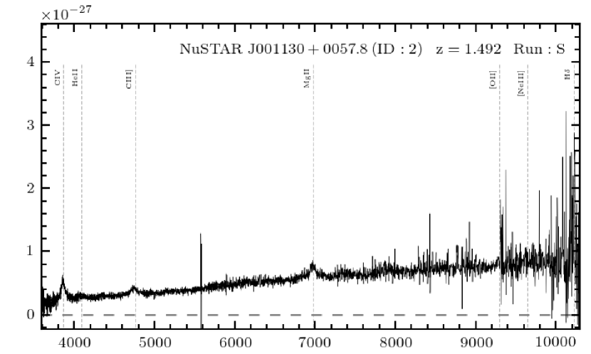
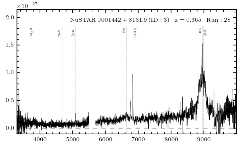
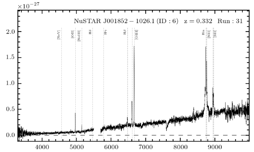
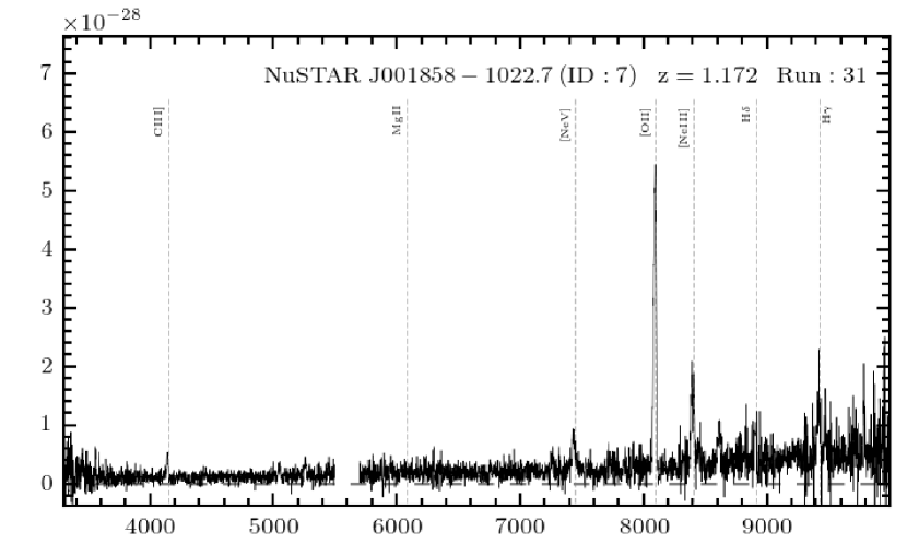
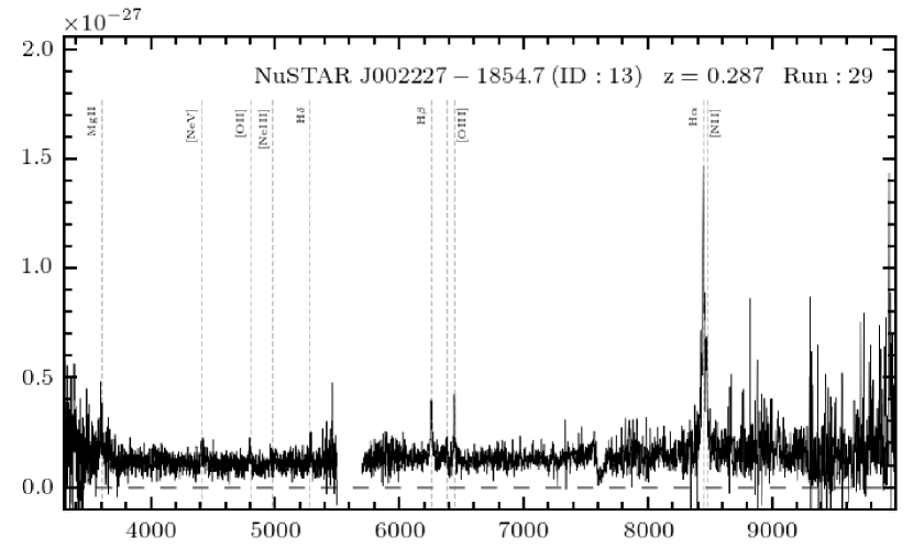
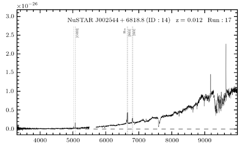
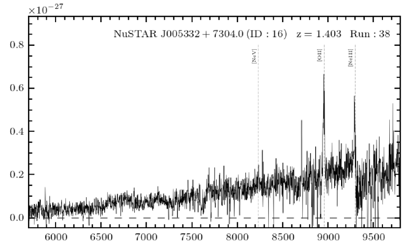
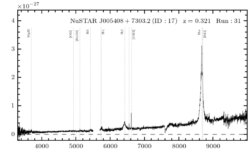
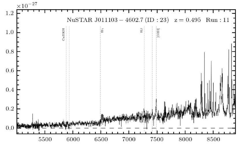
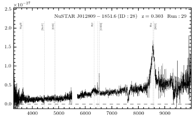
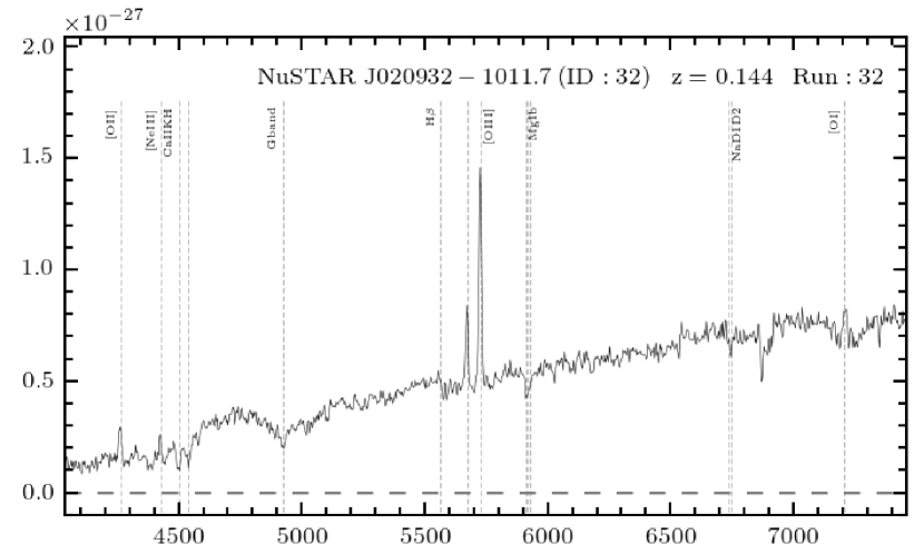
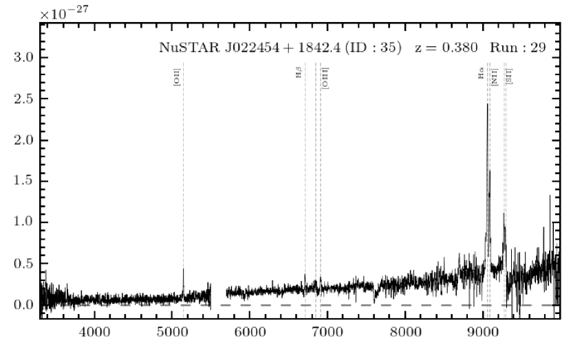
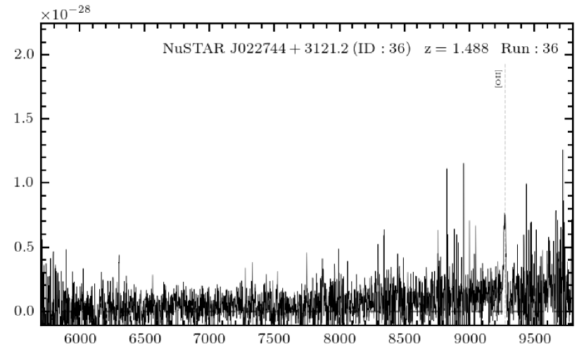
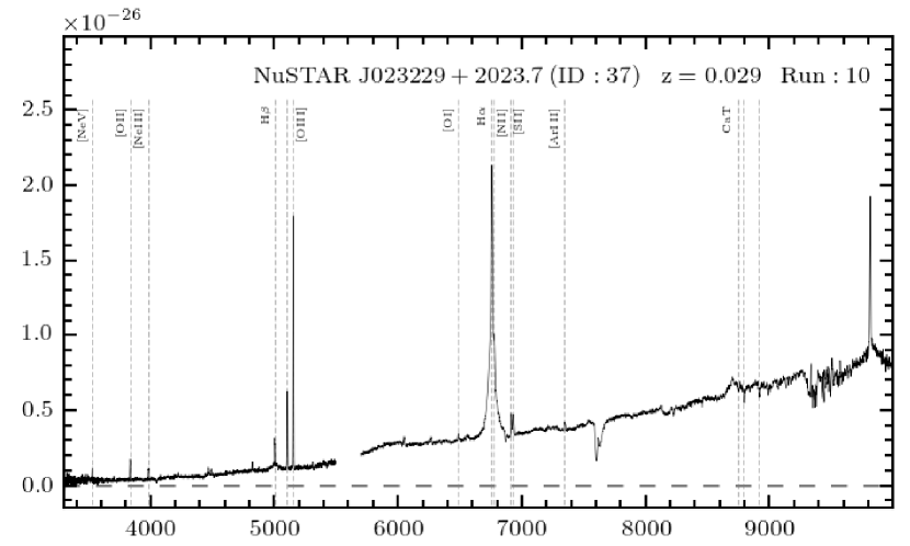
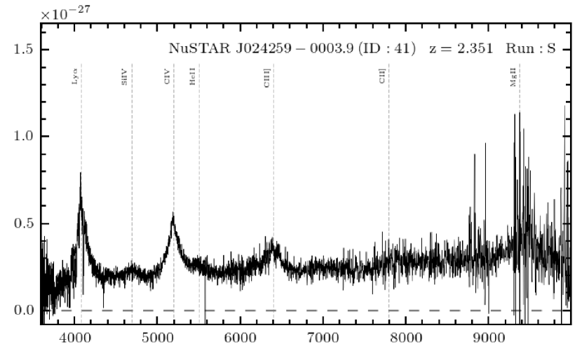
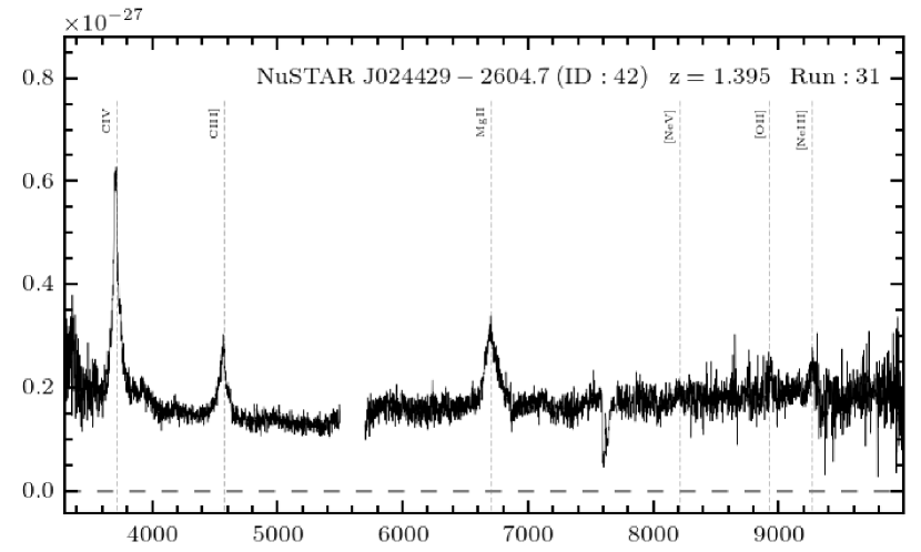
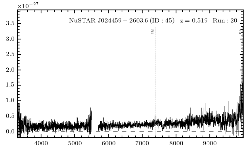
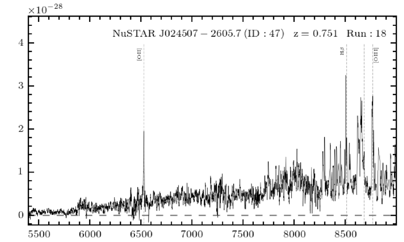
Figure 21.— Optical spectra for the NuSTAR serendipitous survey sources (continued on the following pages). The horizontal axis shows the wavelength in units of Å, and the vertical axis shows the flux ($f_{\mathrm{\nu}}$) in units of erg s^-1 cm^-2 Hz^-1. Shown in the upper right corner are the unique NuSTAR source name, the unique source ID, the source redshift, and the observing run identification number (corresponding to Tables 4 and LABEL:specTable; “S” indicates SDSS spectra). The identified emission and absorption lines are labelled and marked with vertical dashed gray lines. Full resolution figures are available online.

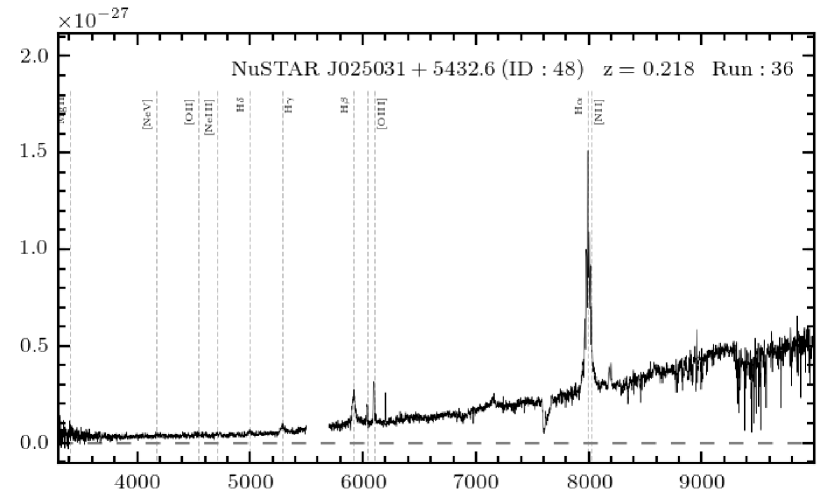
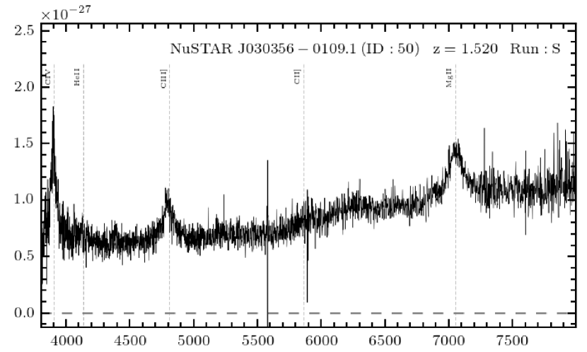
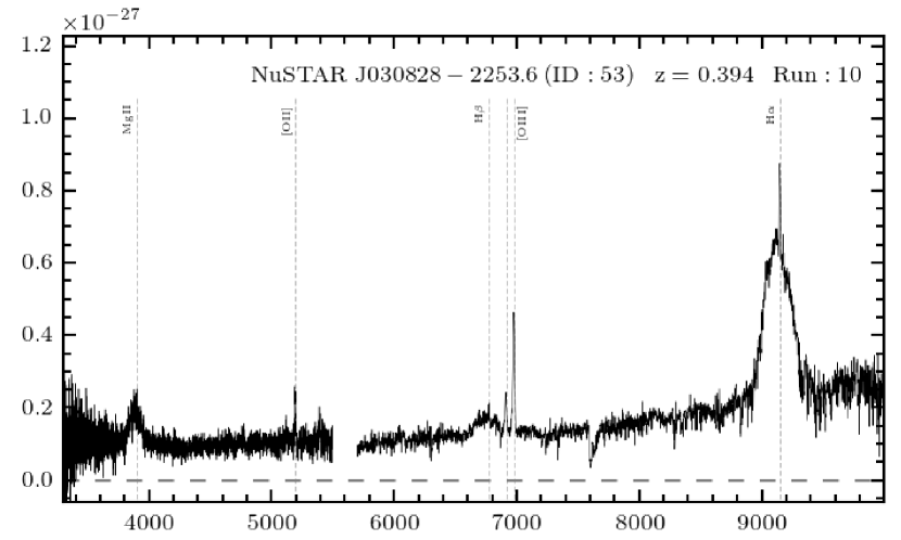
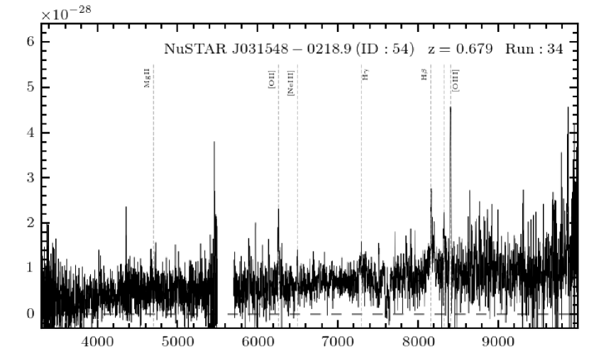
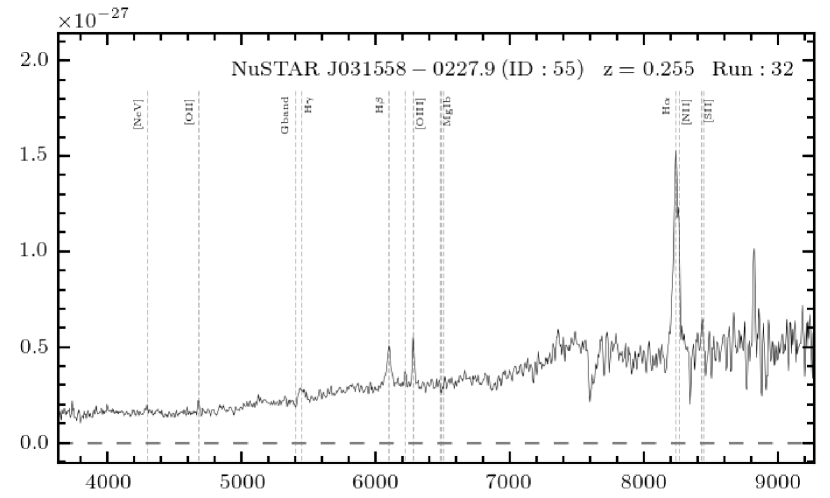
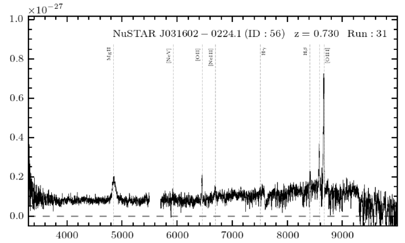
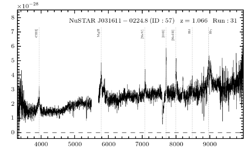
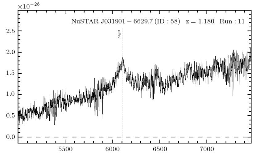
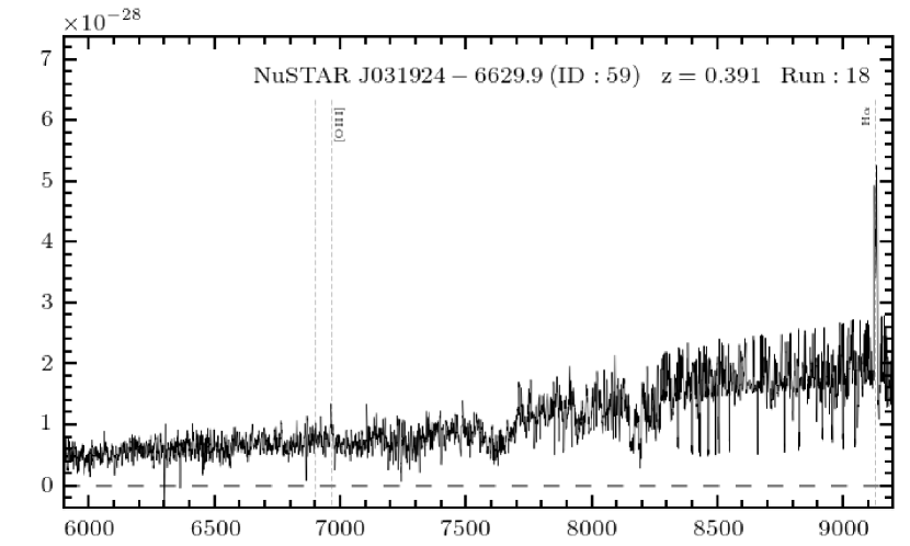
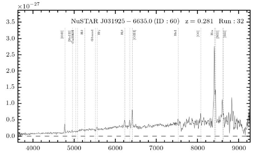
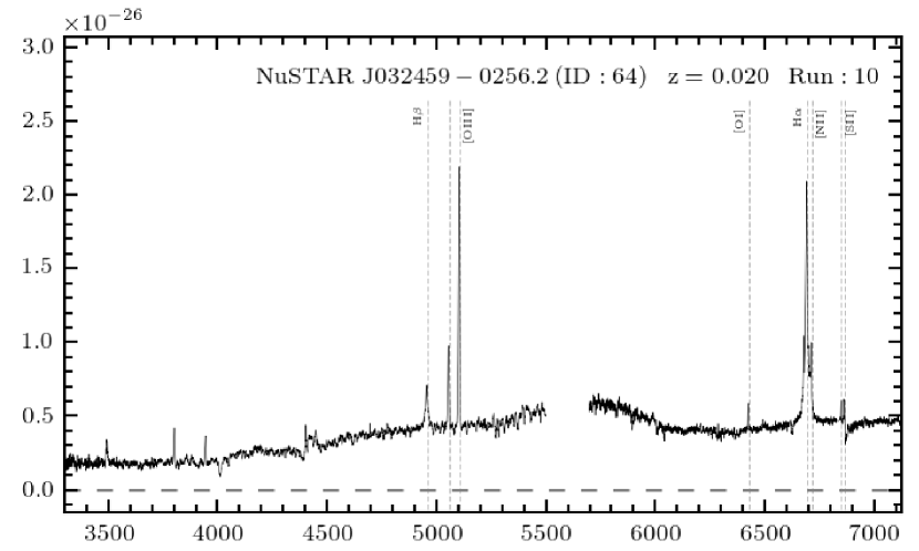
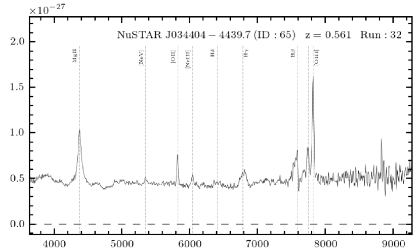
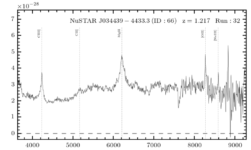
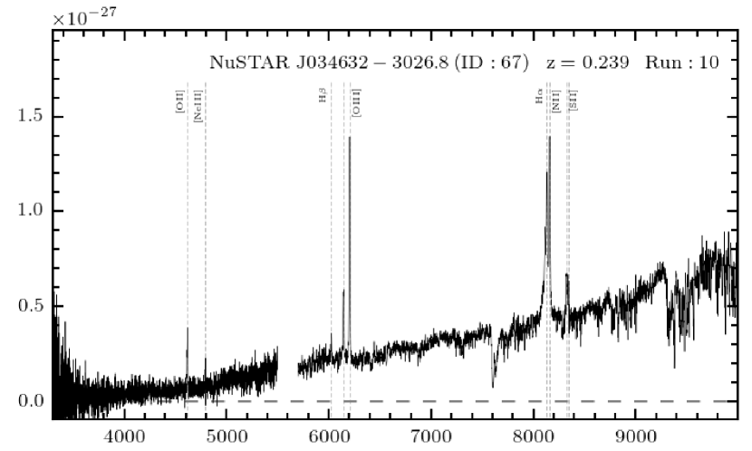
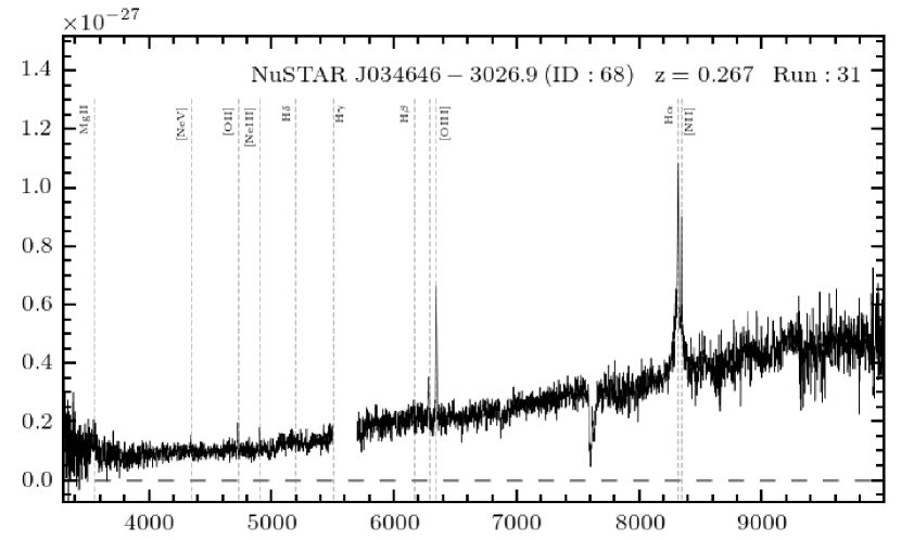
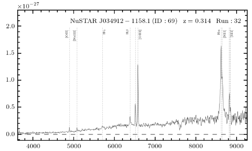
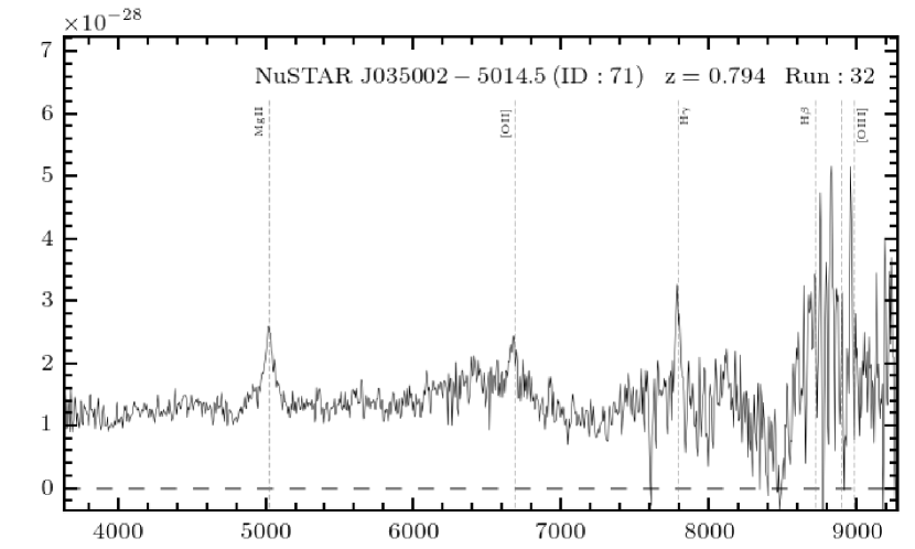
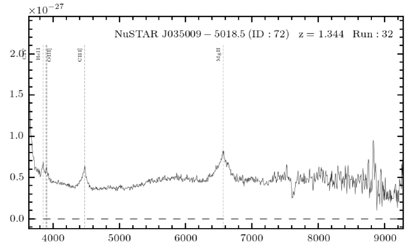
Figure 21.— Continued.

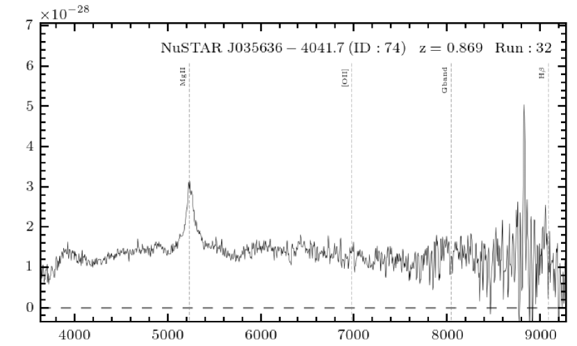
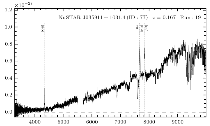
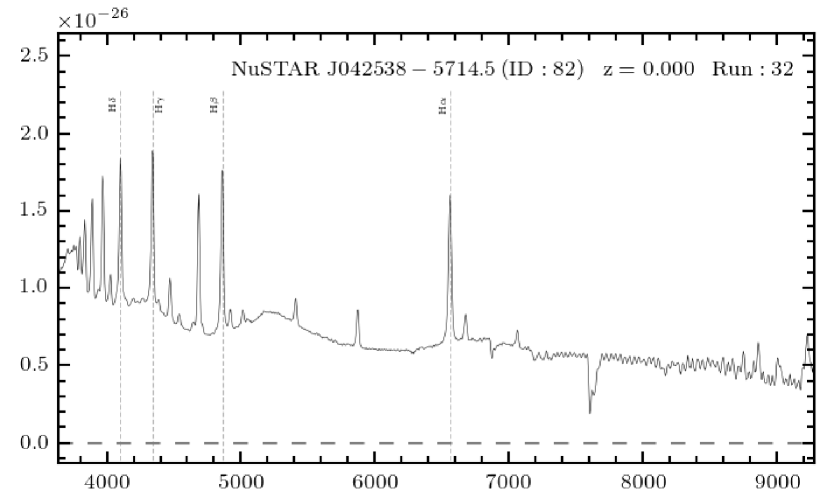
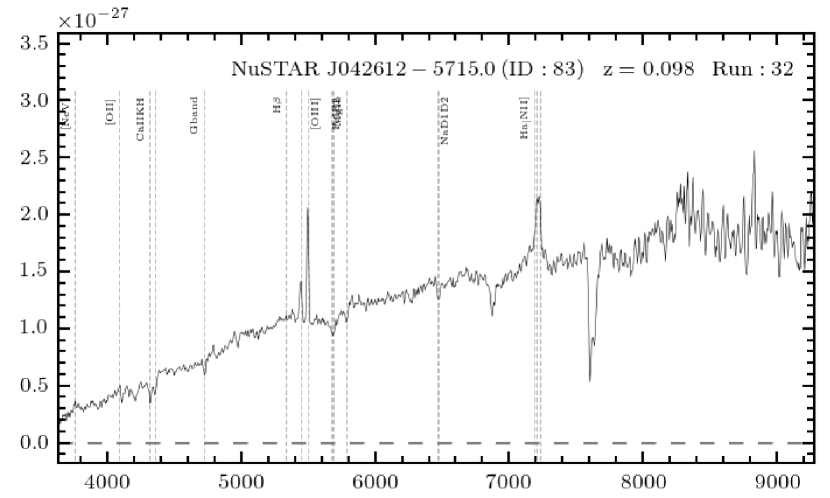
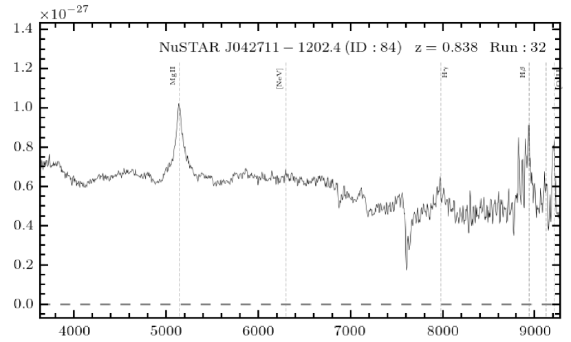
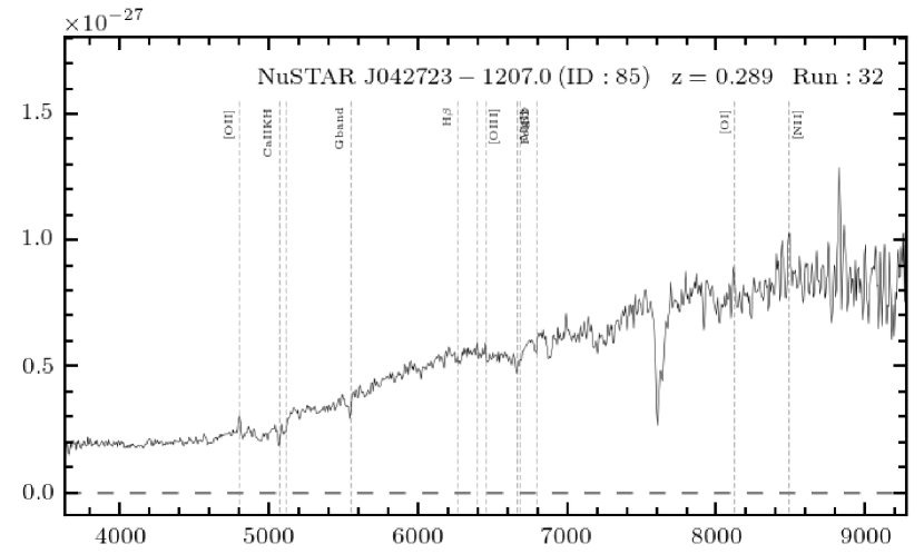
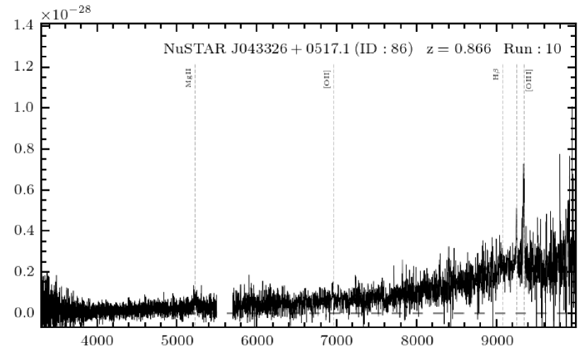
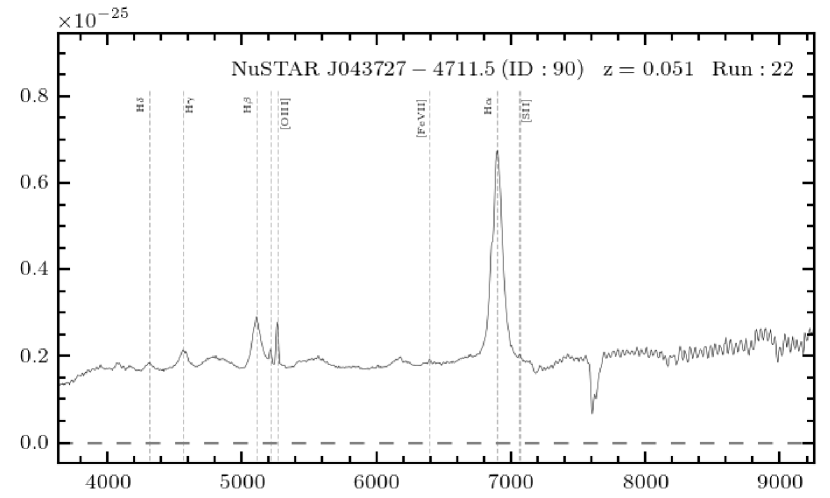
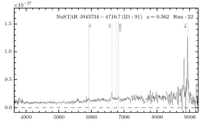
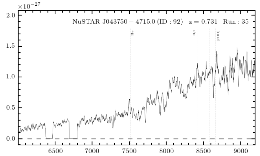
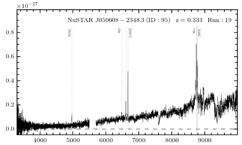
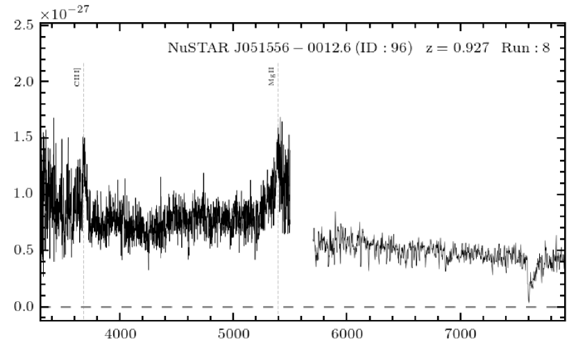
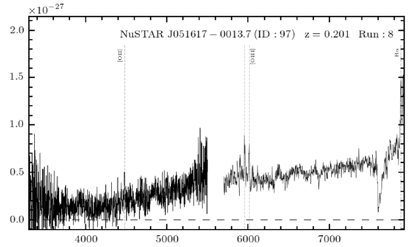
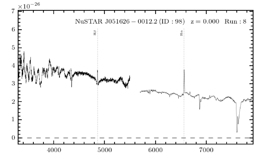
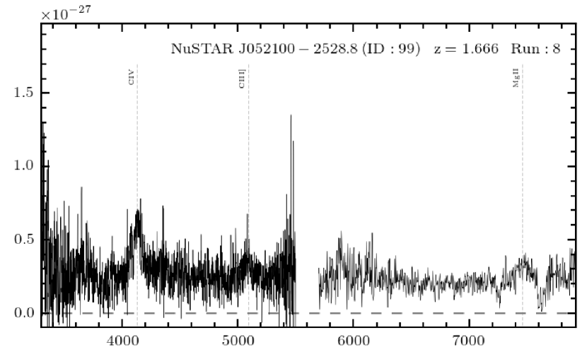
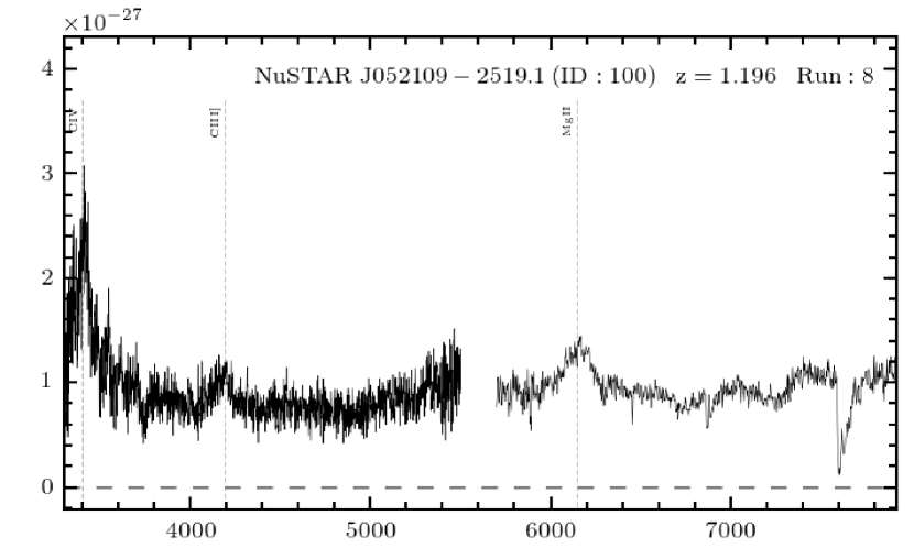
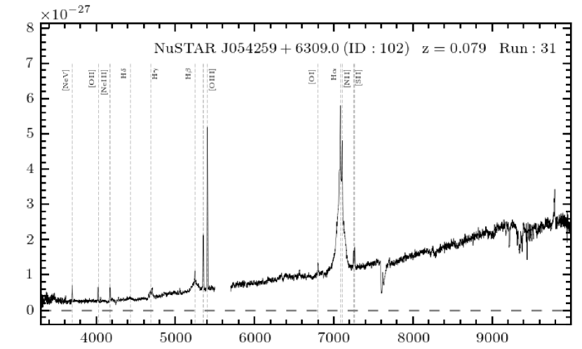
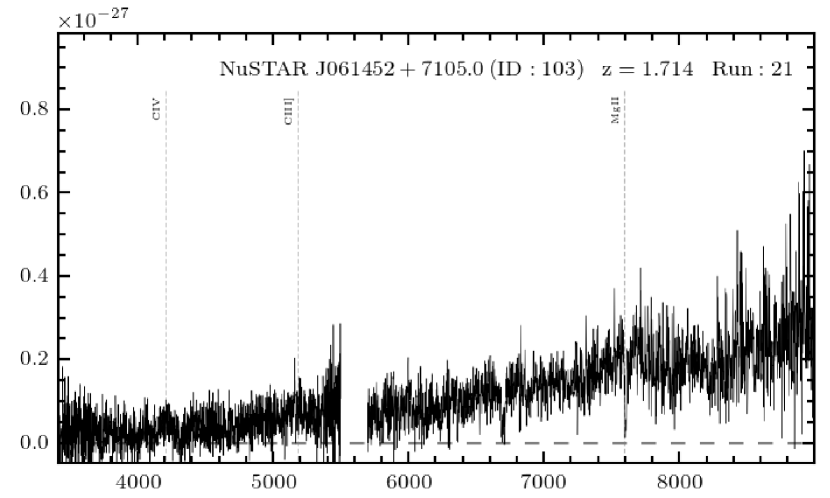
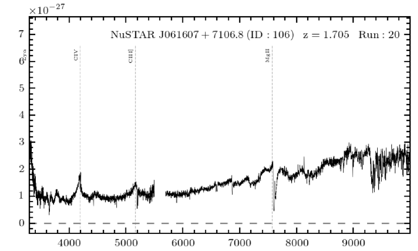
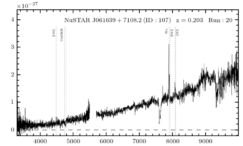
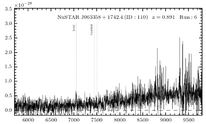
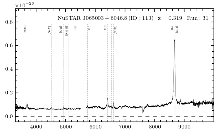
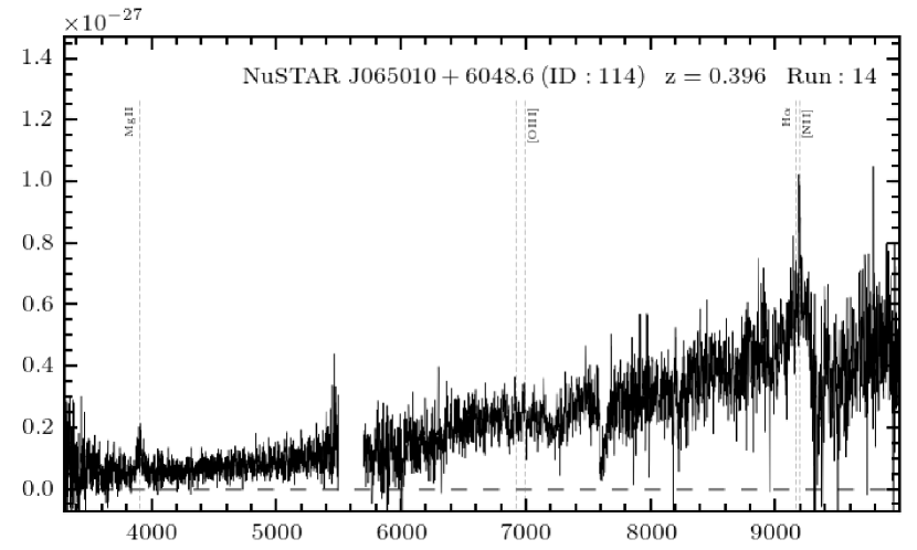
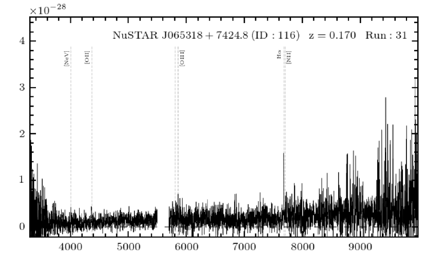
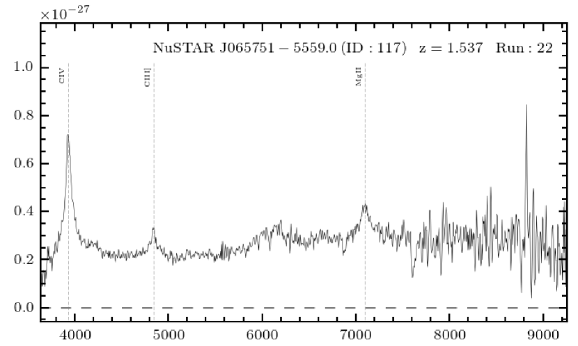
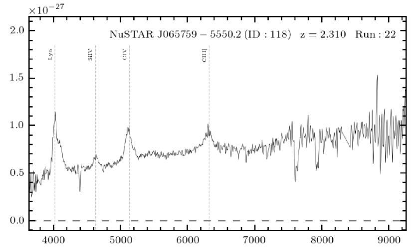
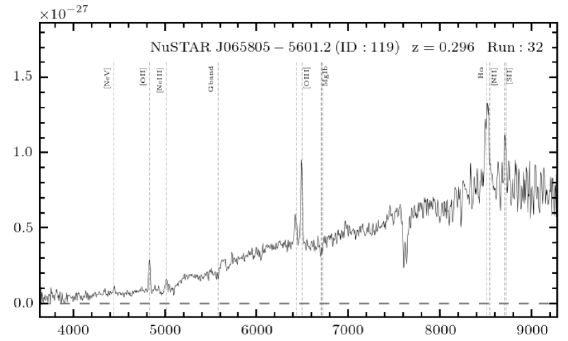
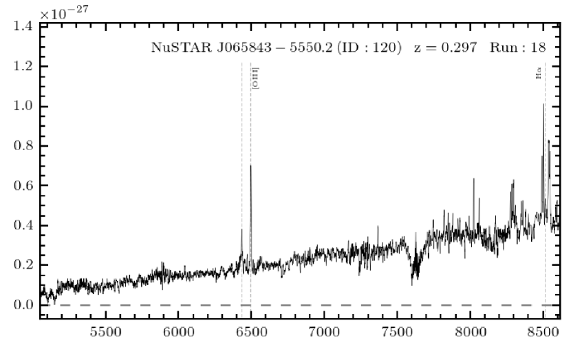
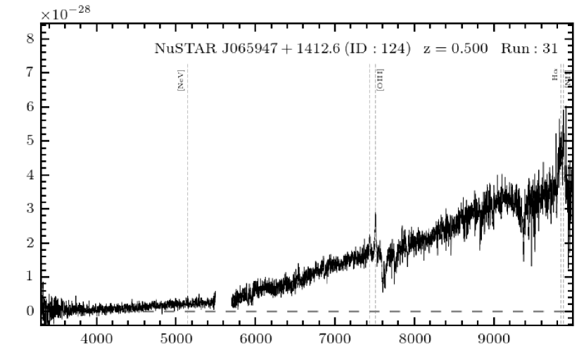
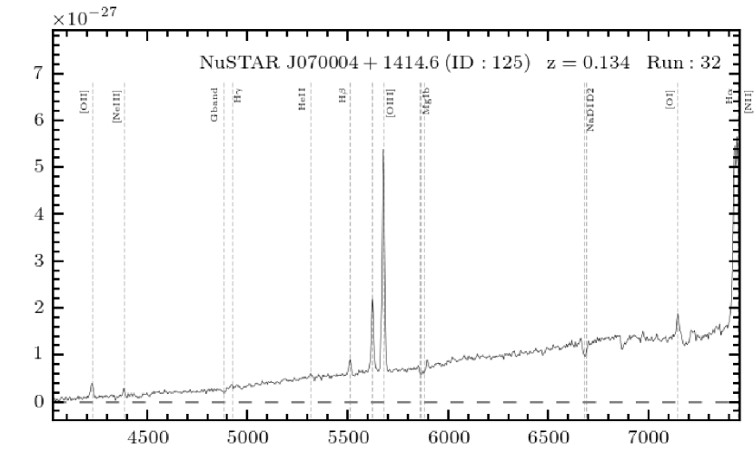
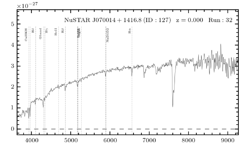
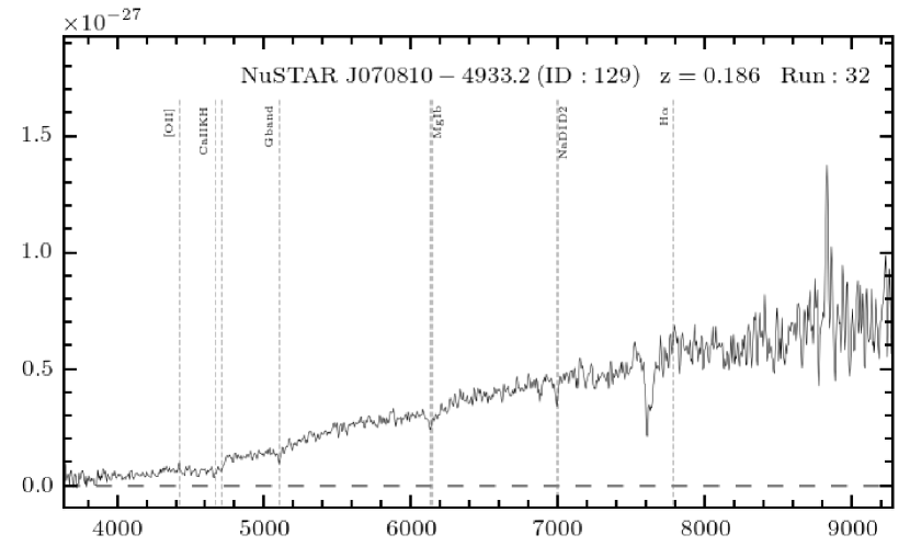
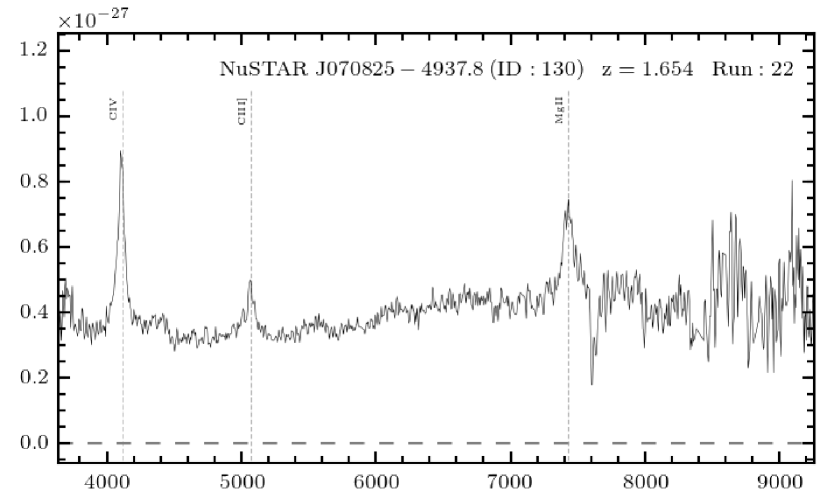
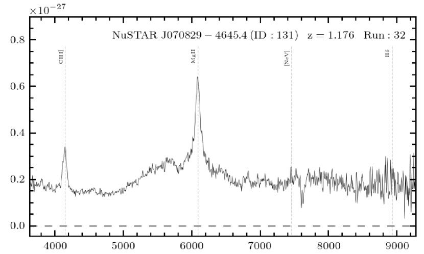
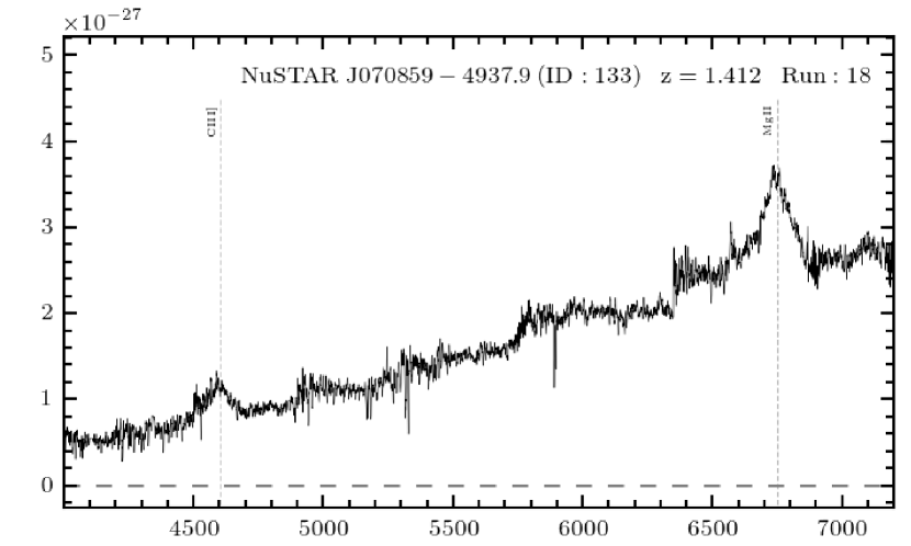
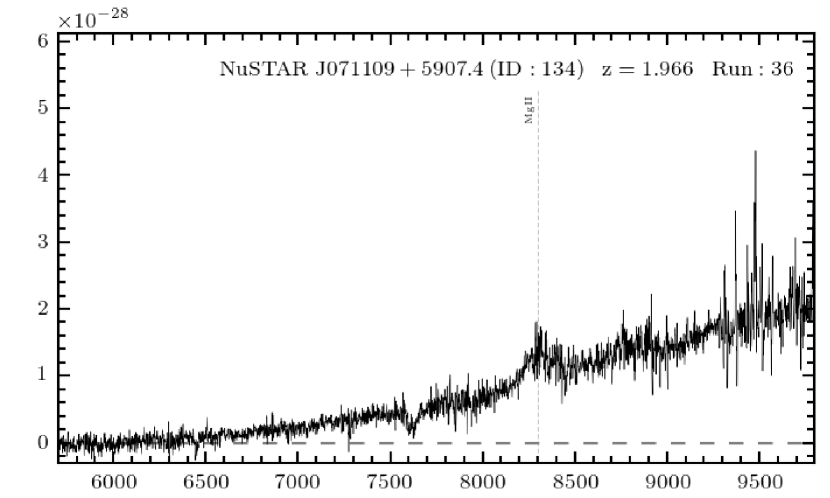
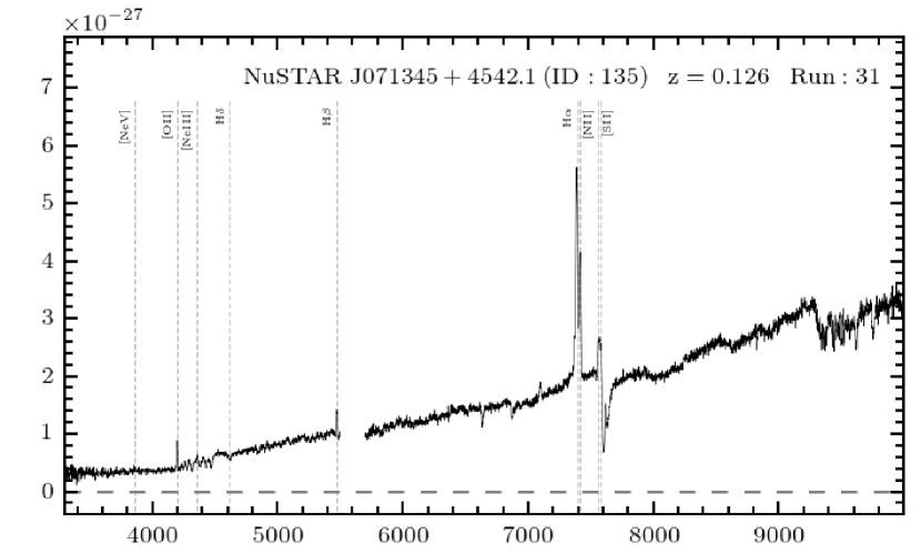
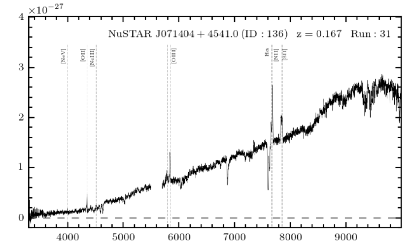
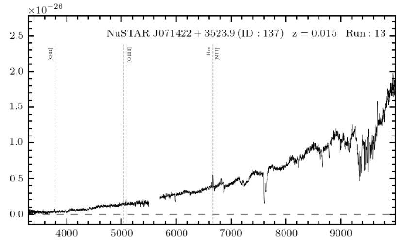
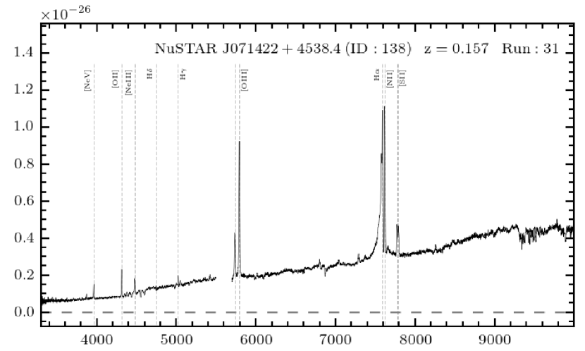
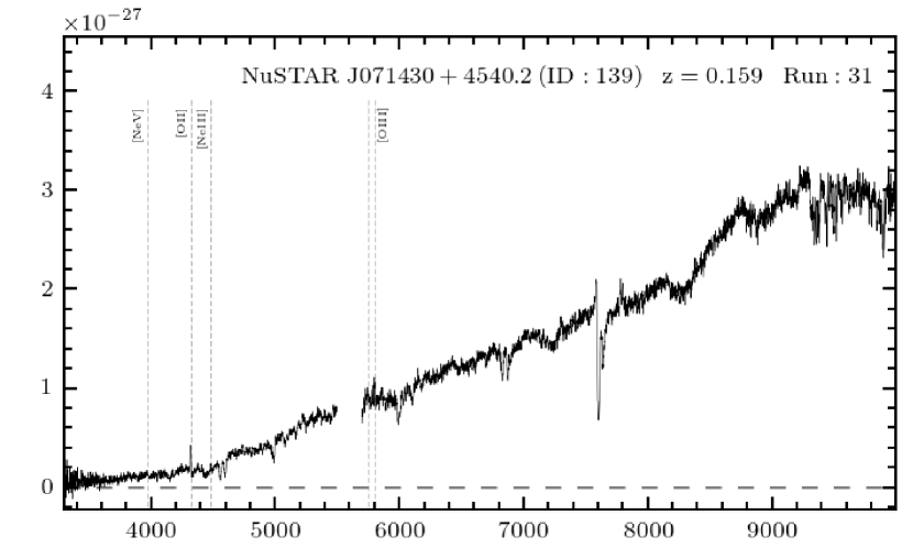
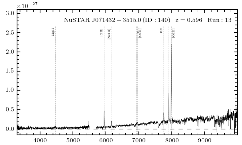
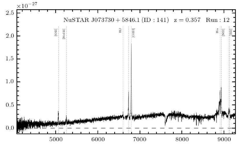
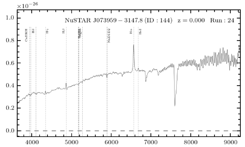
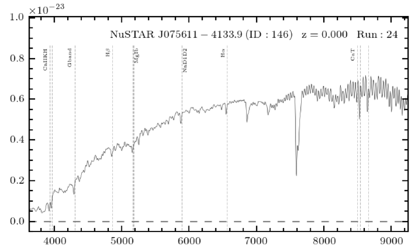
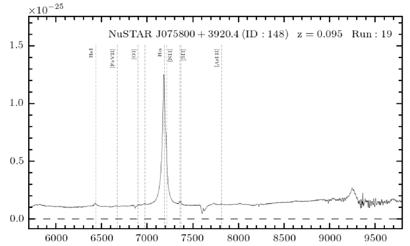
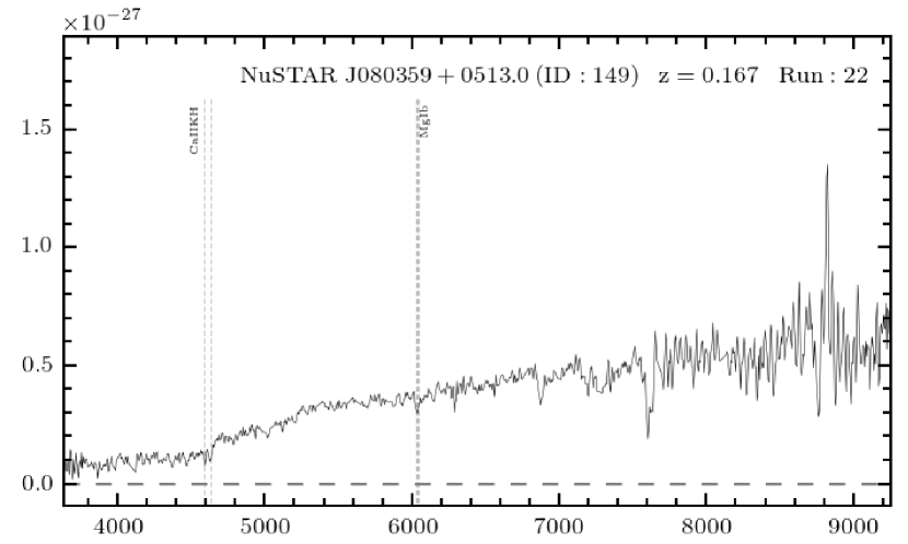
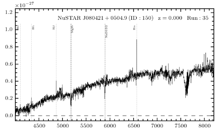
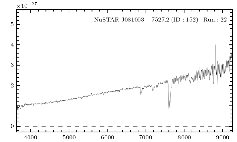
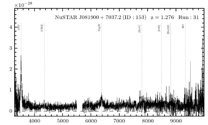
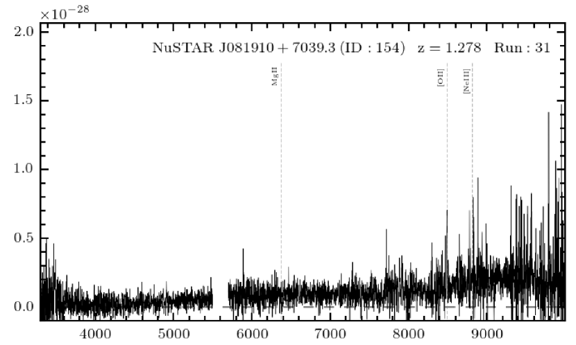
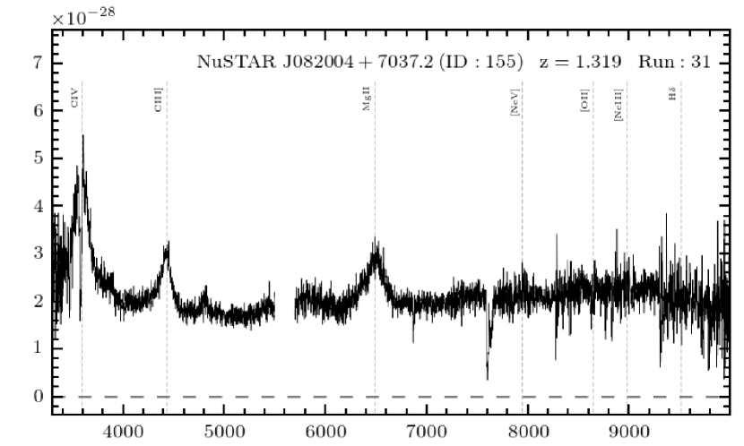
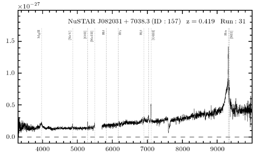
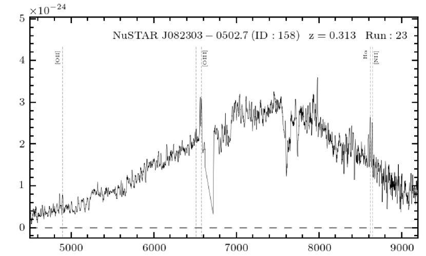
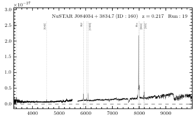
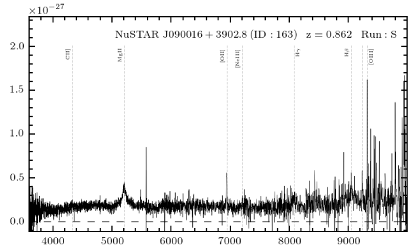
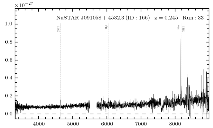
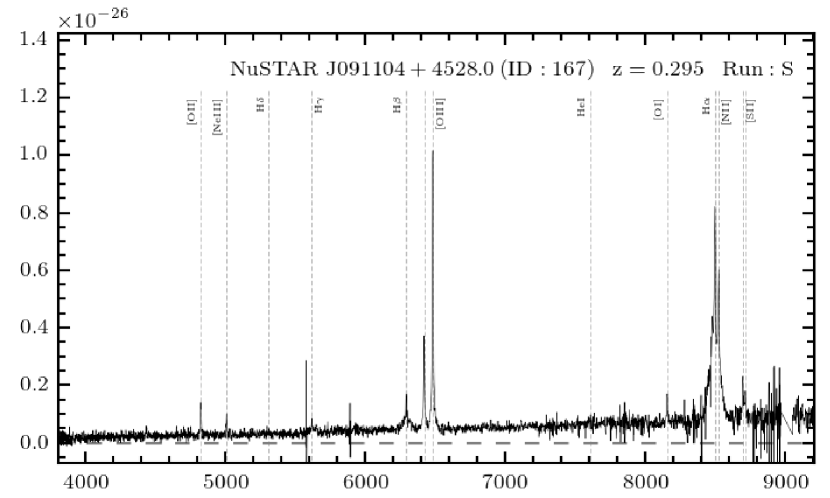
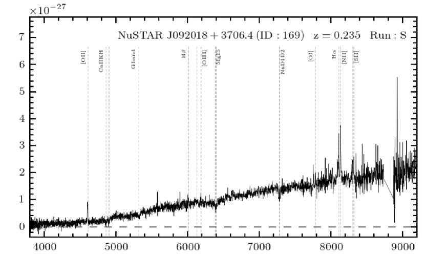
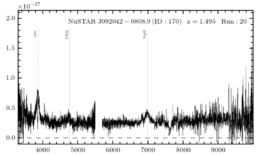
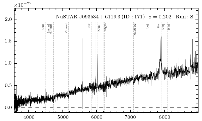
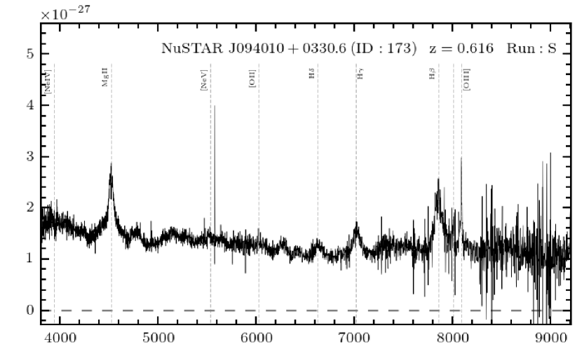
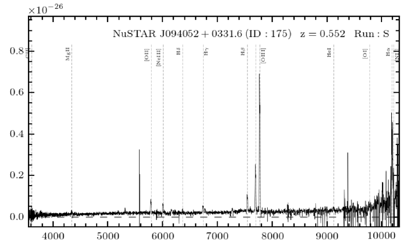
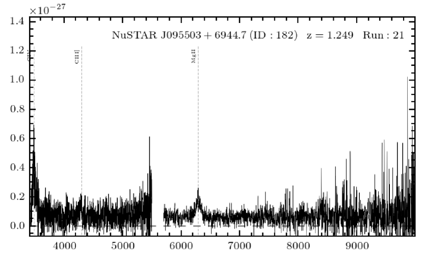
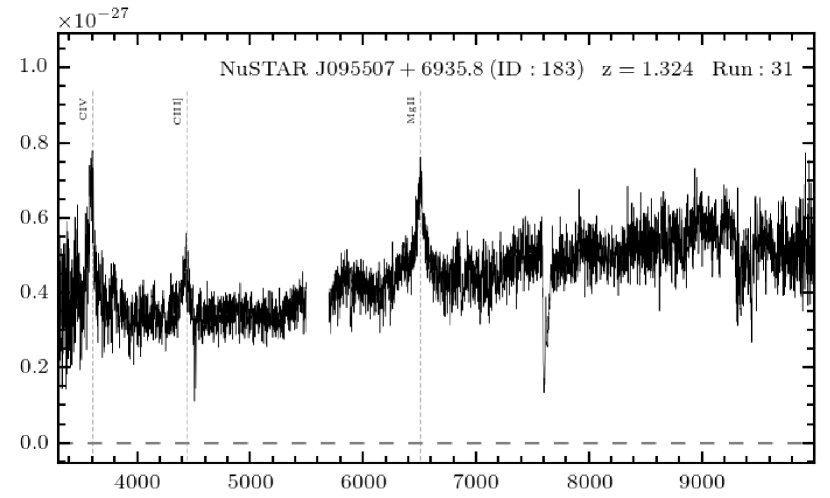
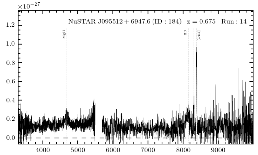
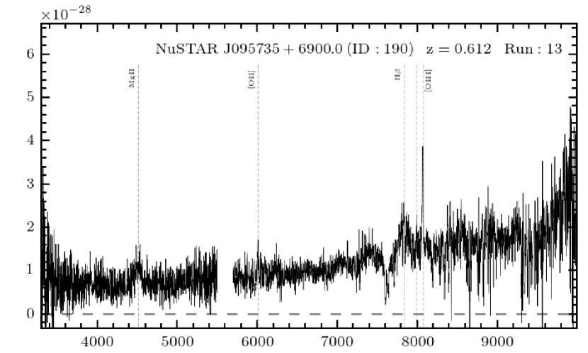
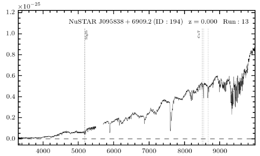
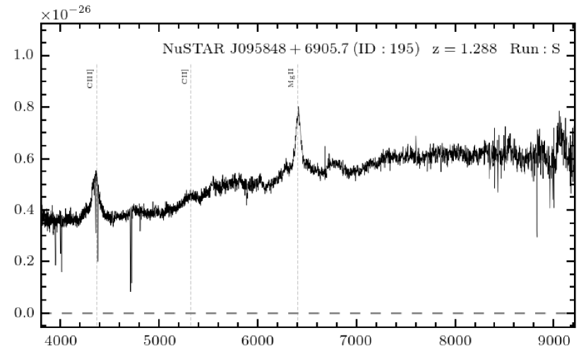
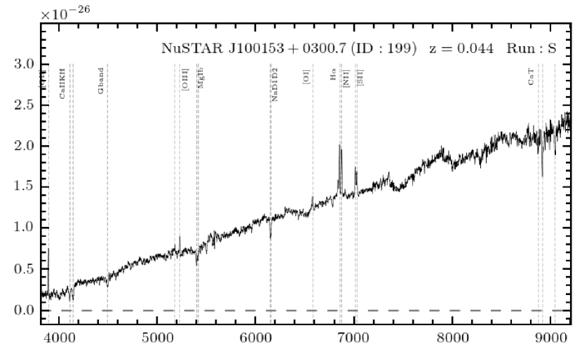
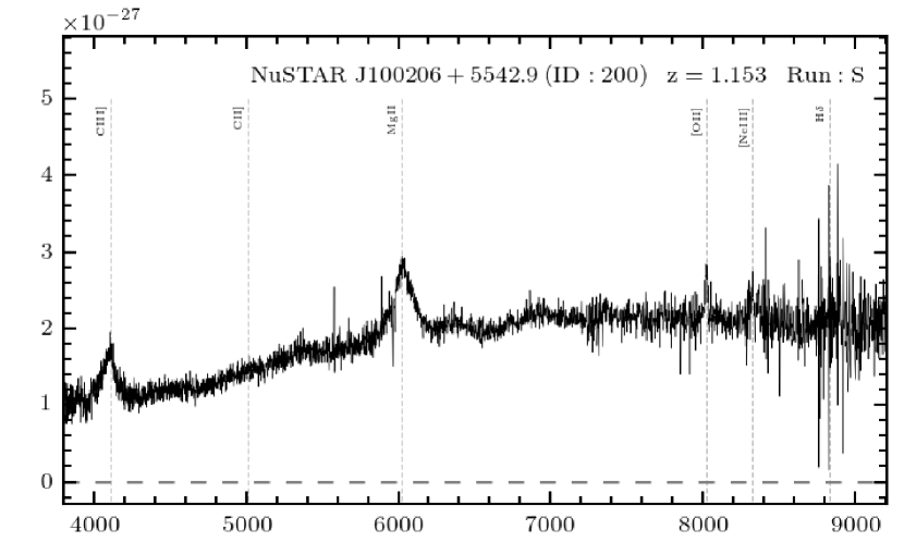
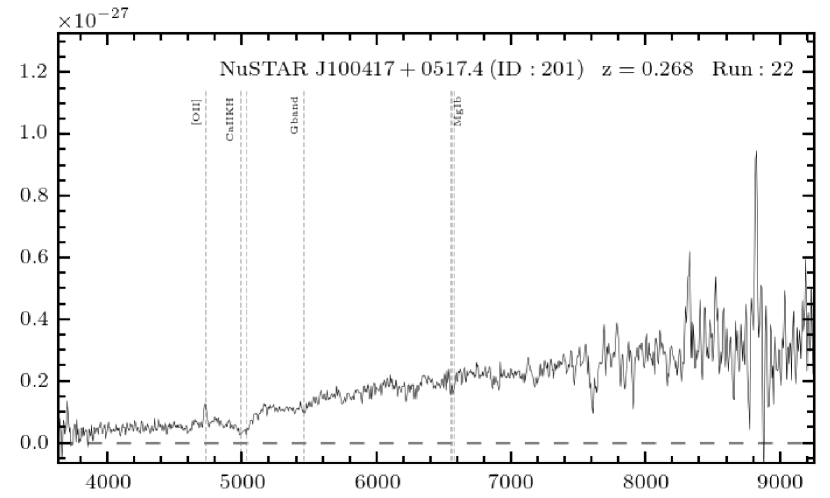
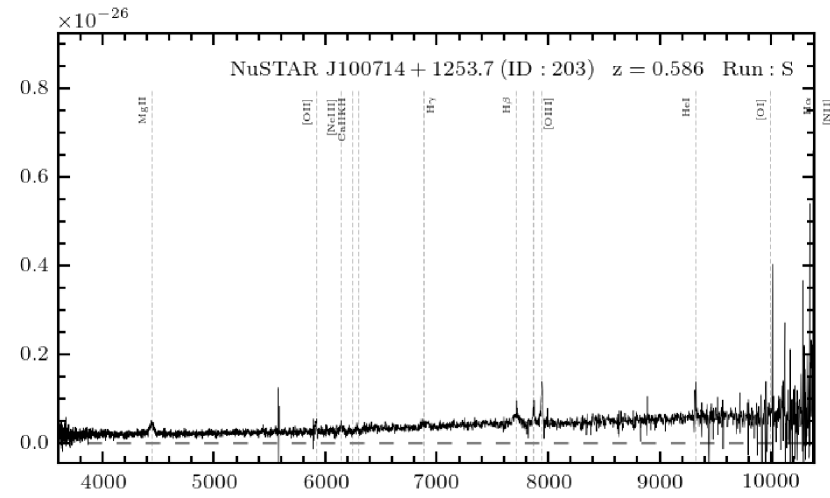
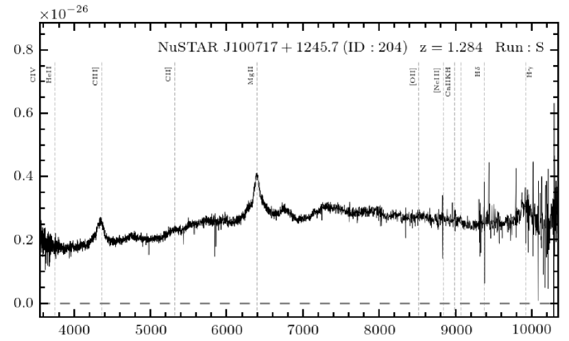
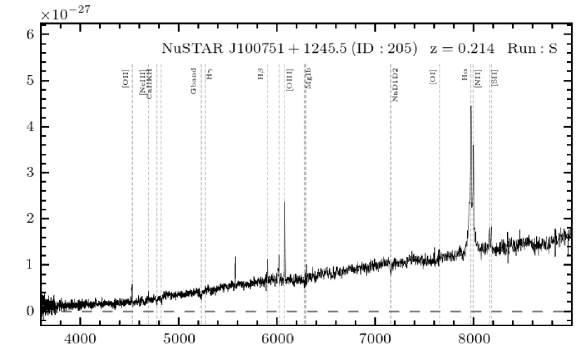
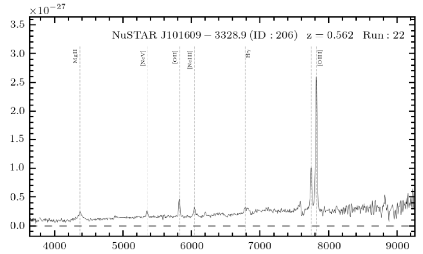
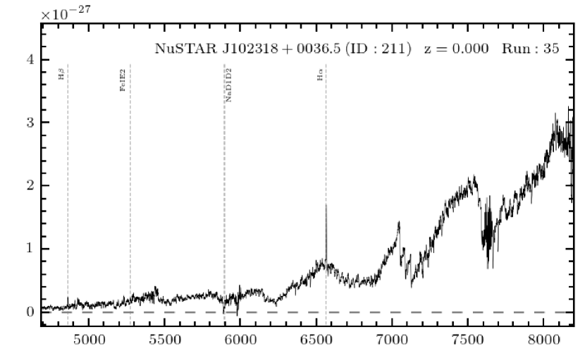
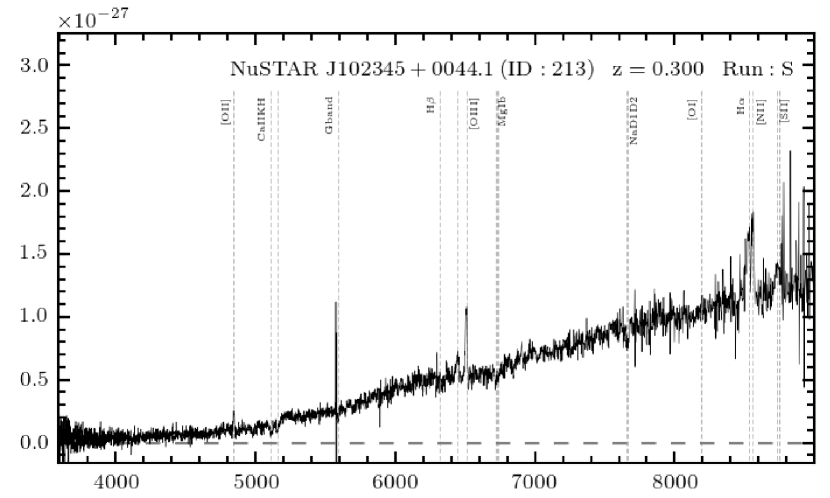
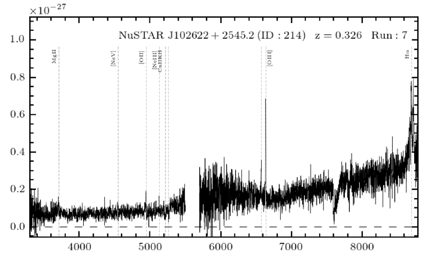
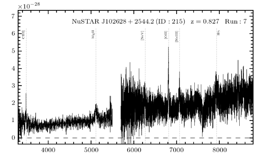
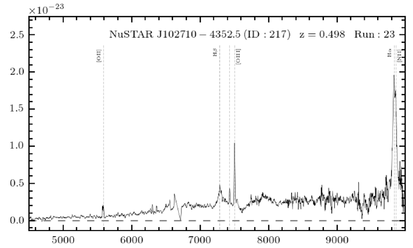
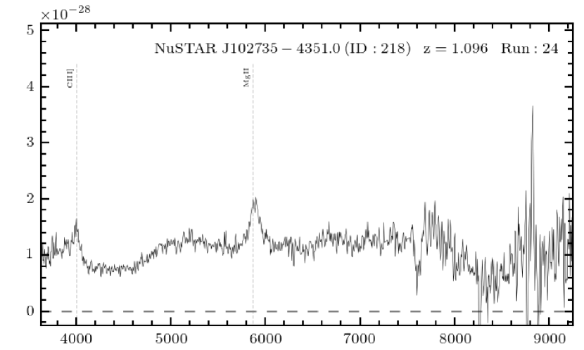
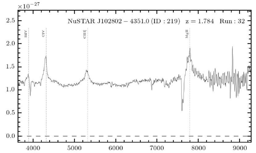
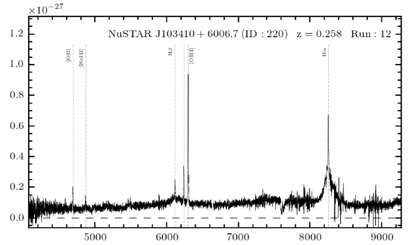
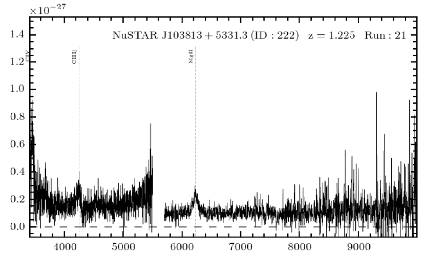
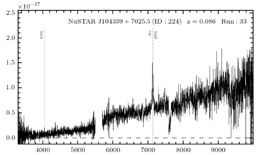
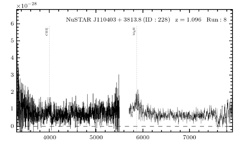
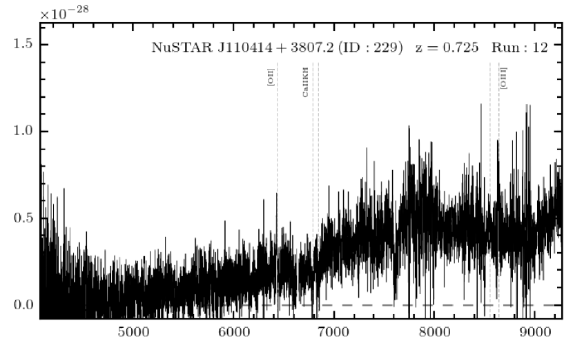
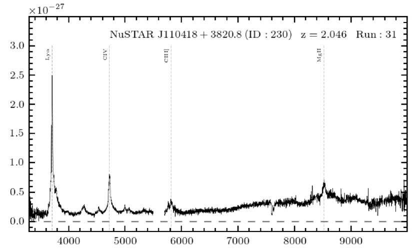
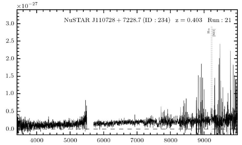
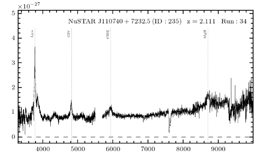
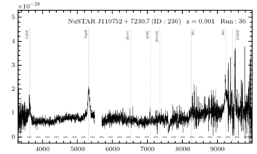
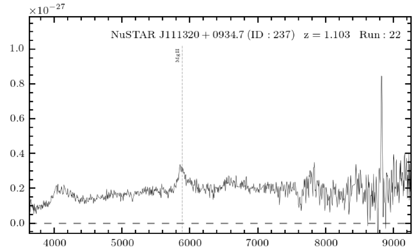
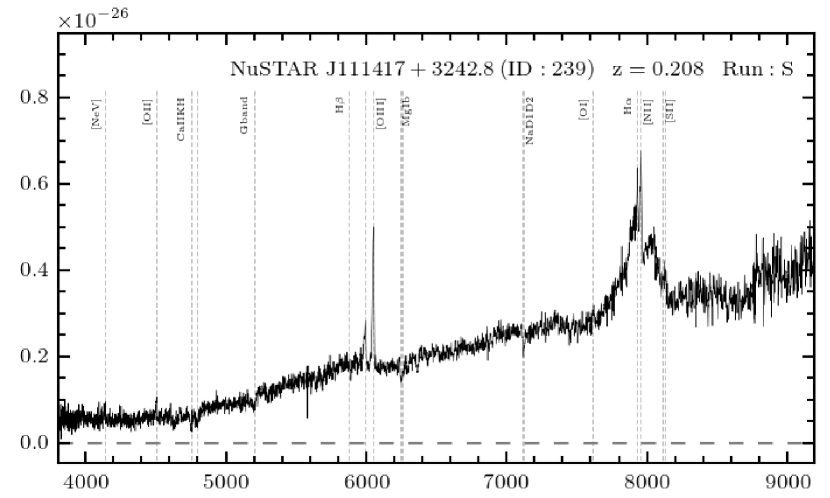
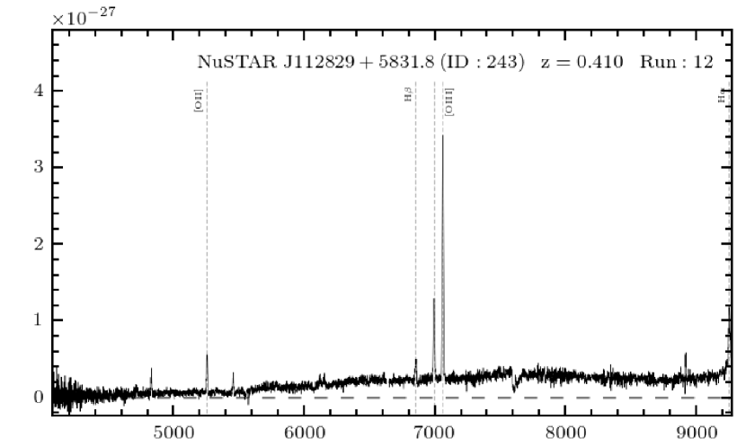
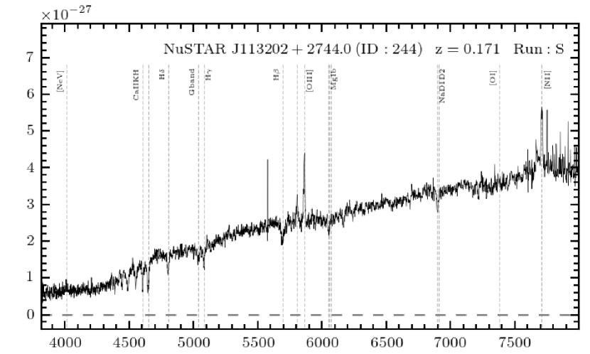
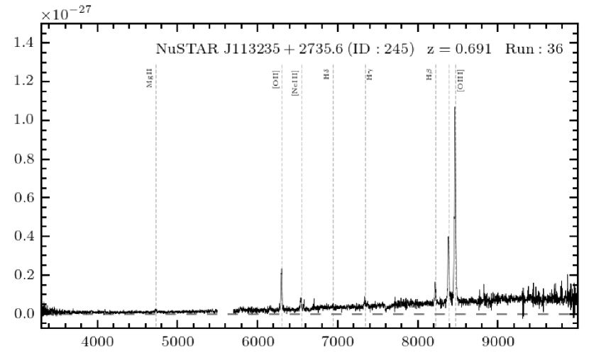
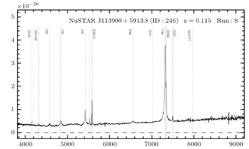
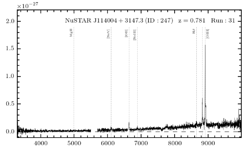
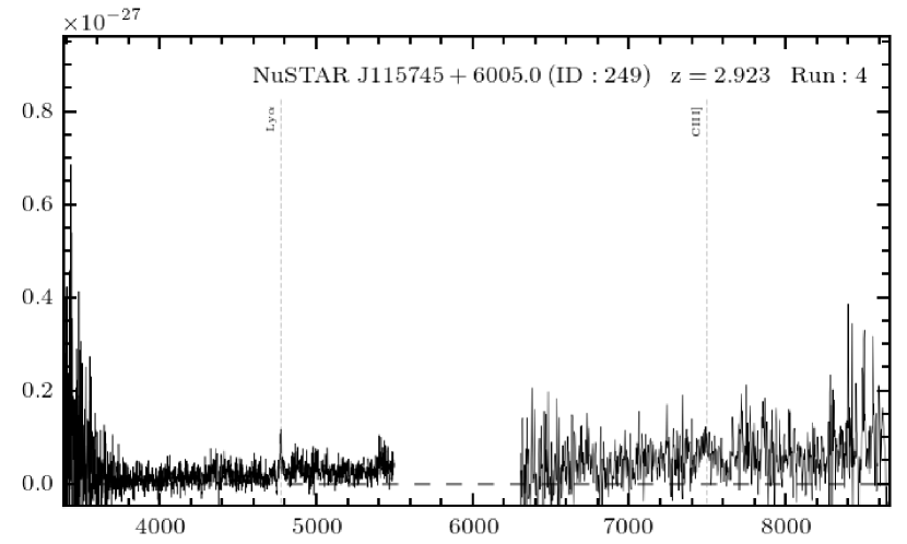
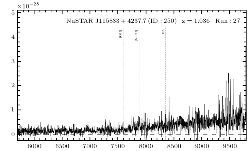
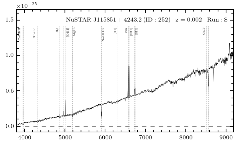
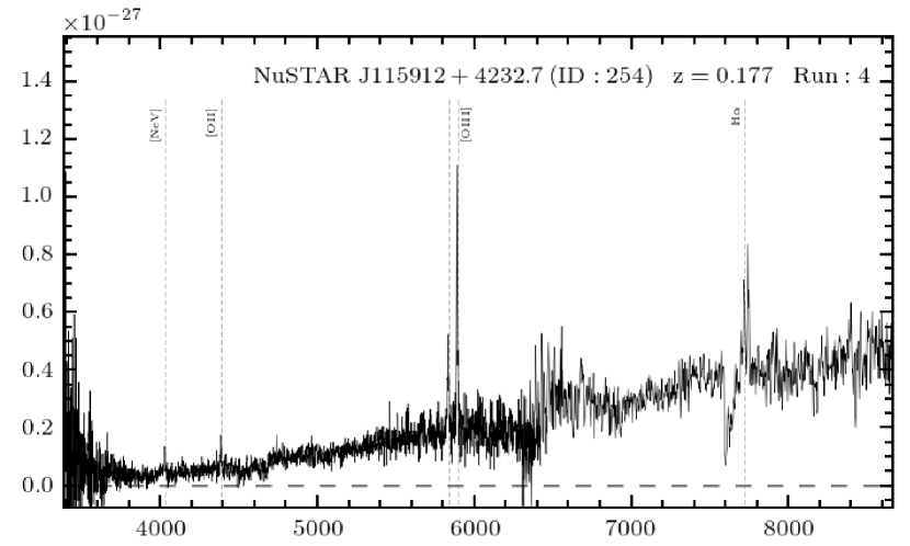
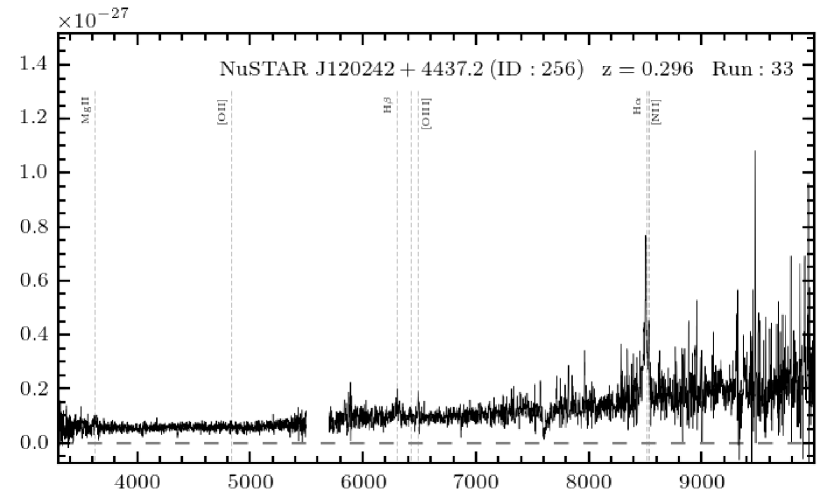
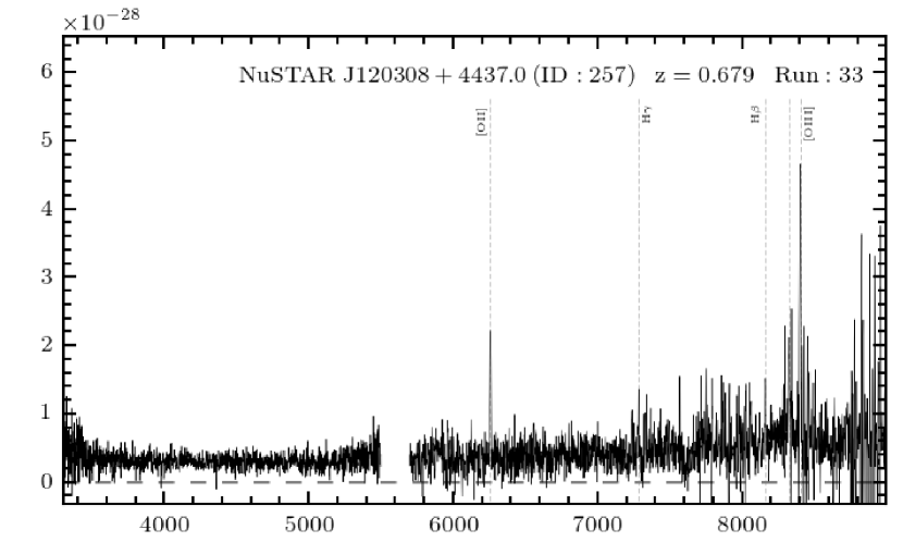
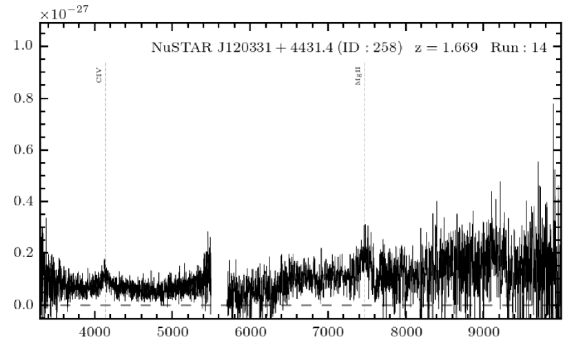
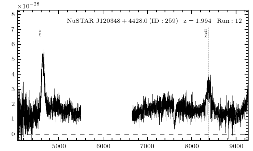
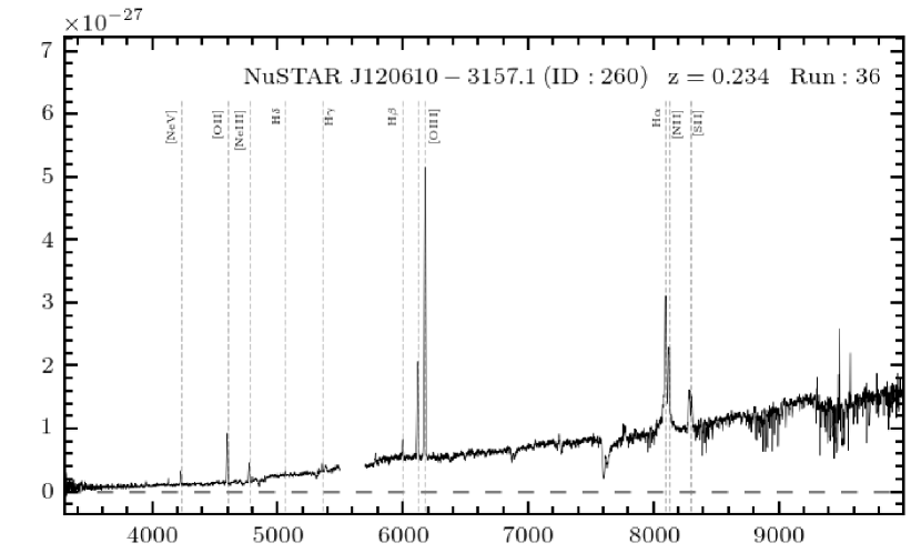
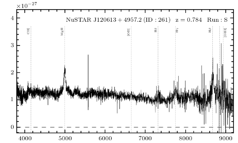
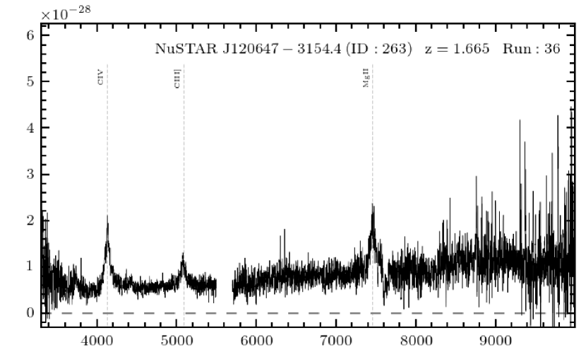
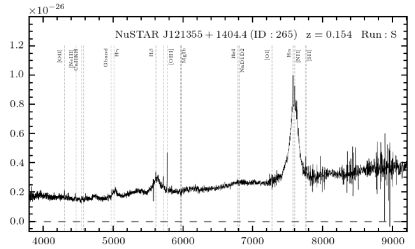
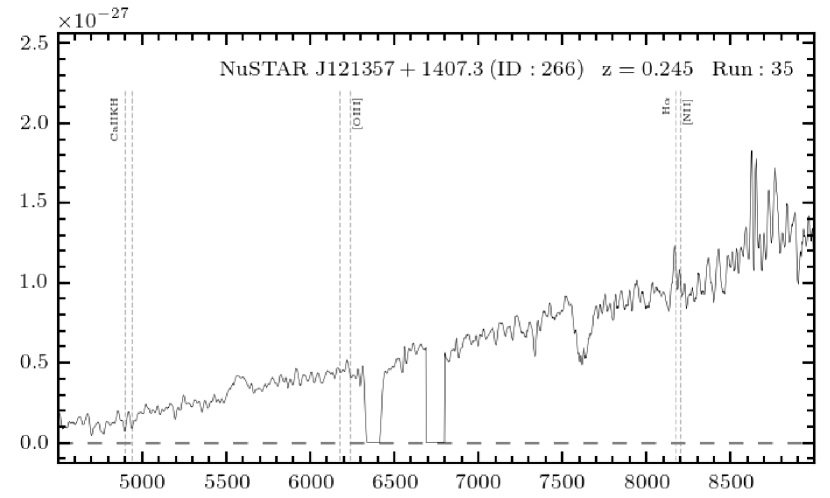
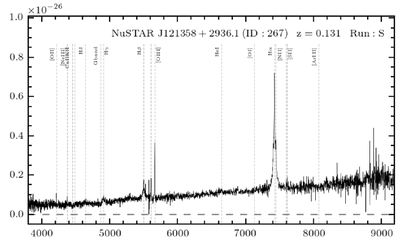
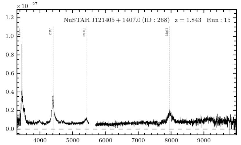
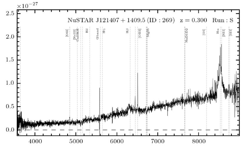
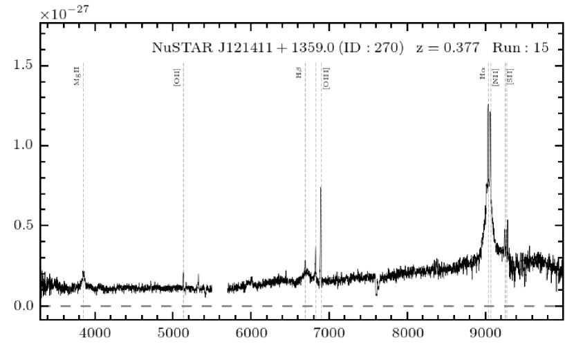
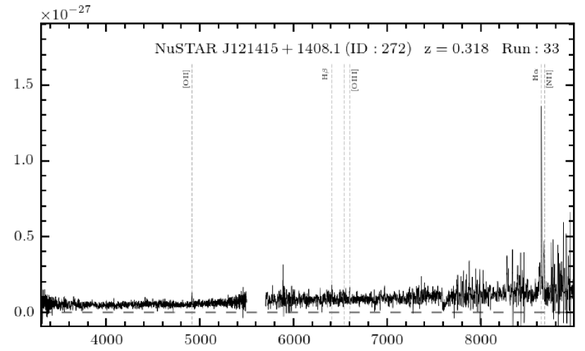
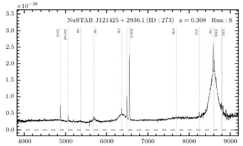
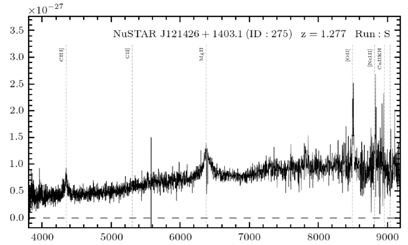
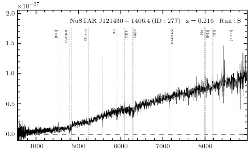
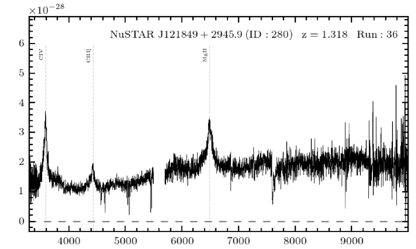
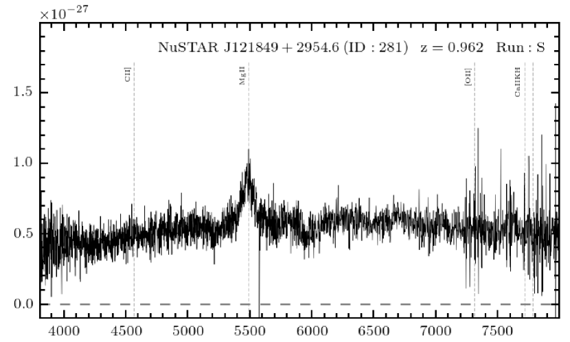
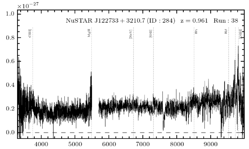
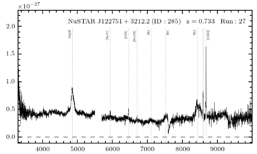
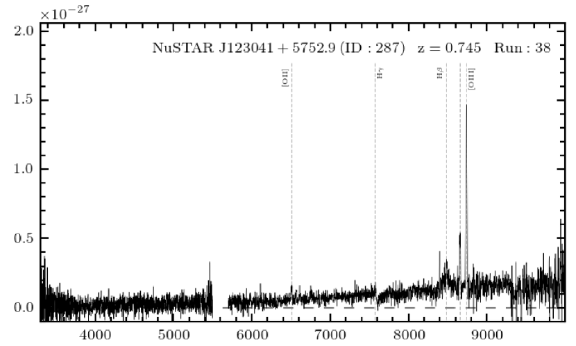
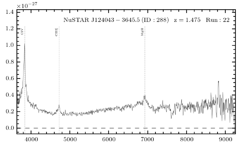
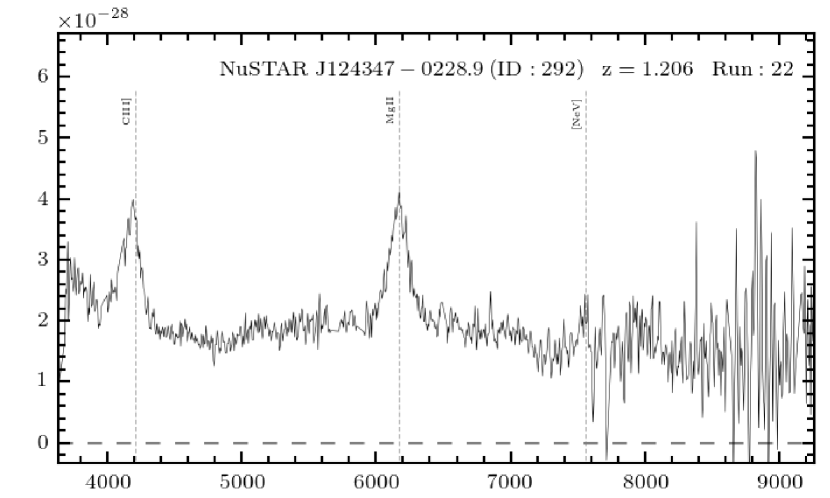
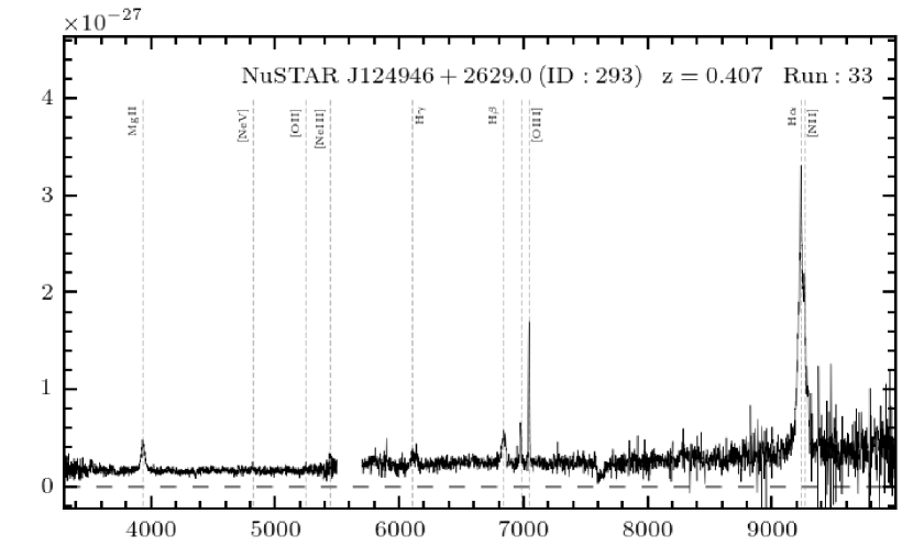
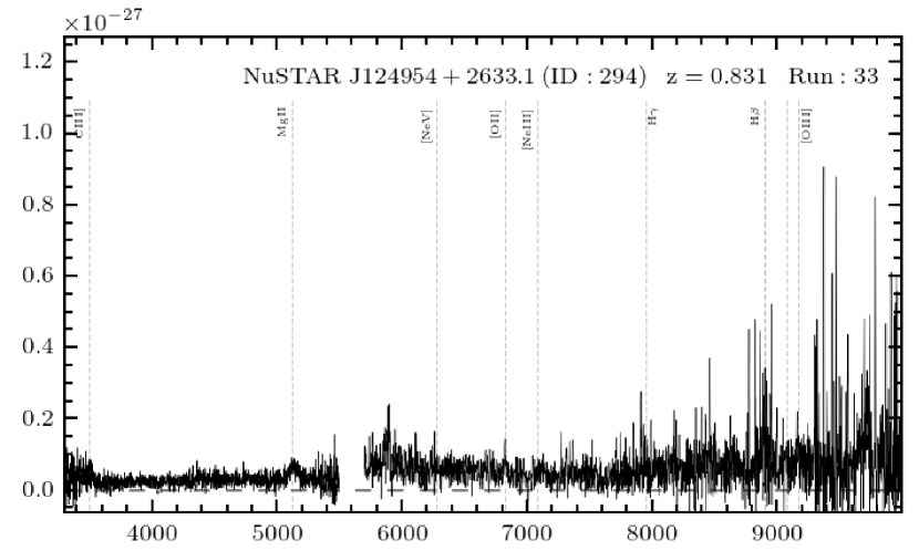
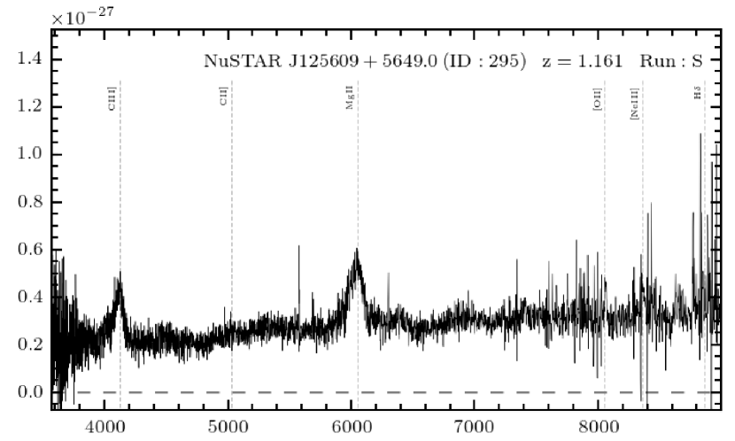
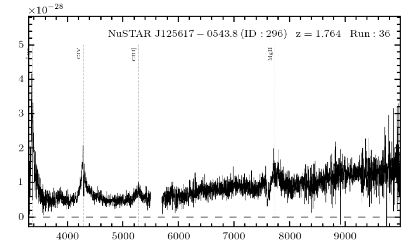
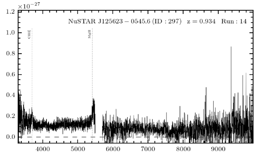
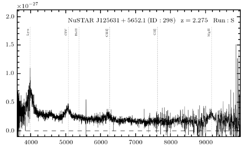
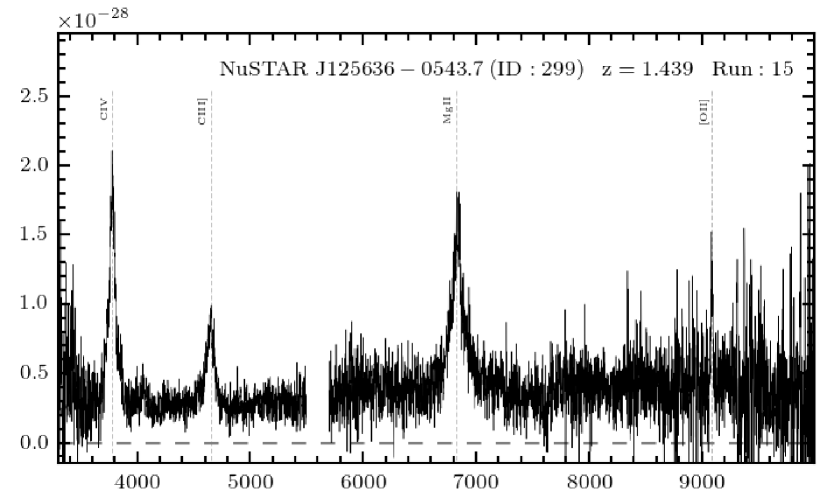
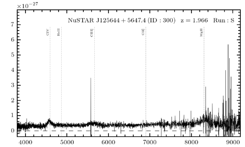
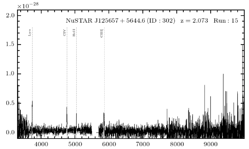
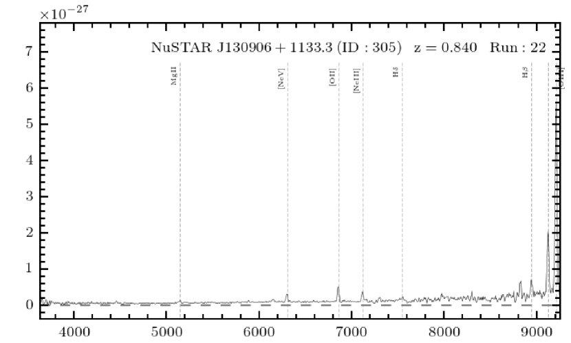
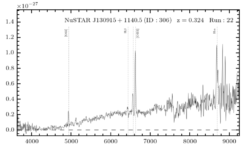
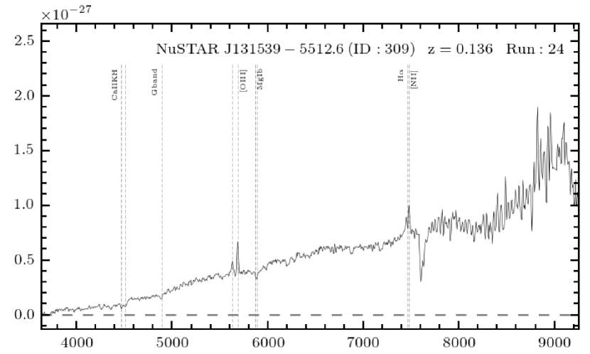
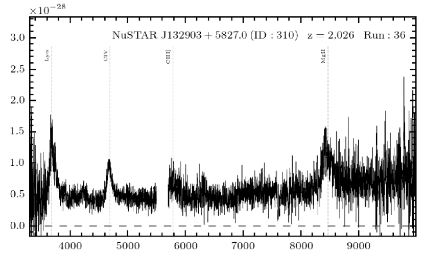
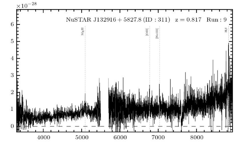
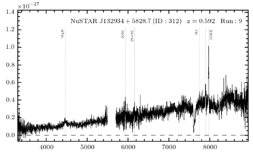
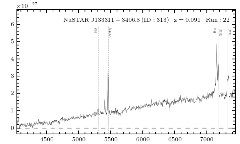
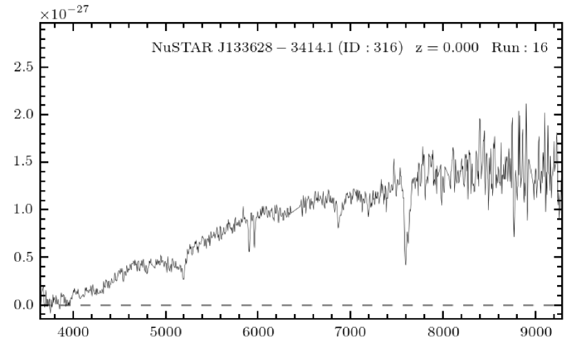
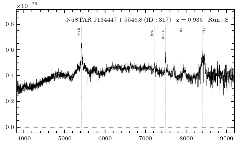
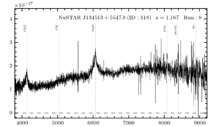
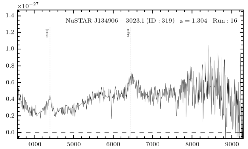
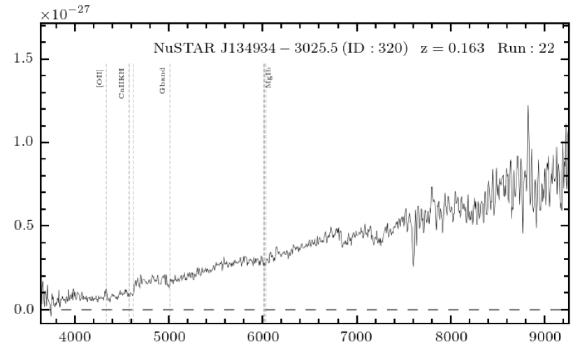
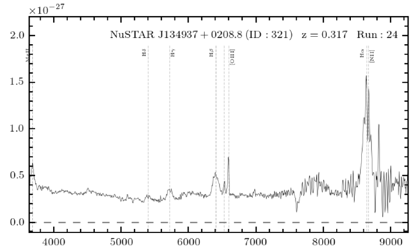
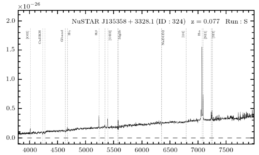
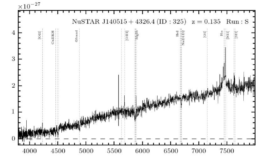
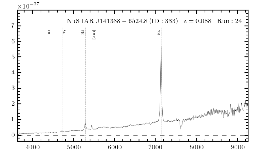
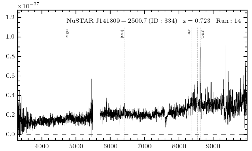
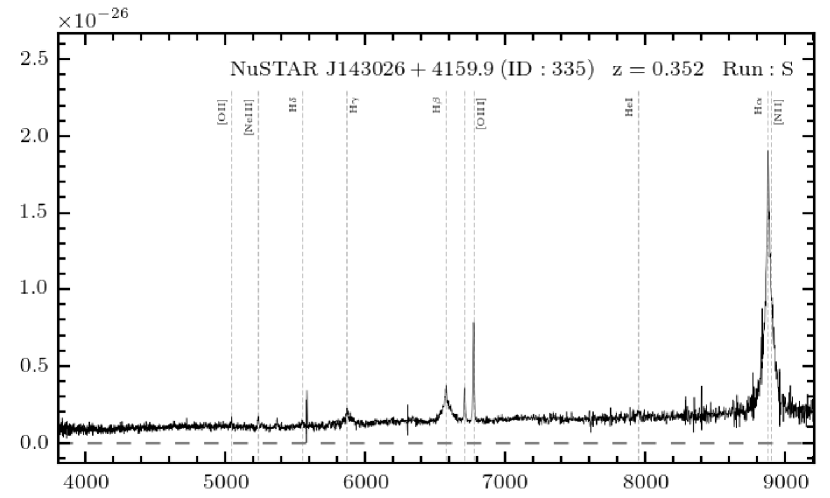
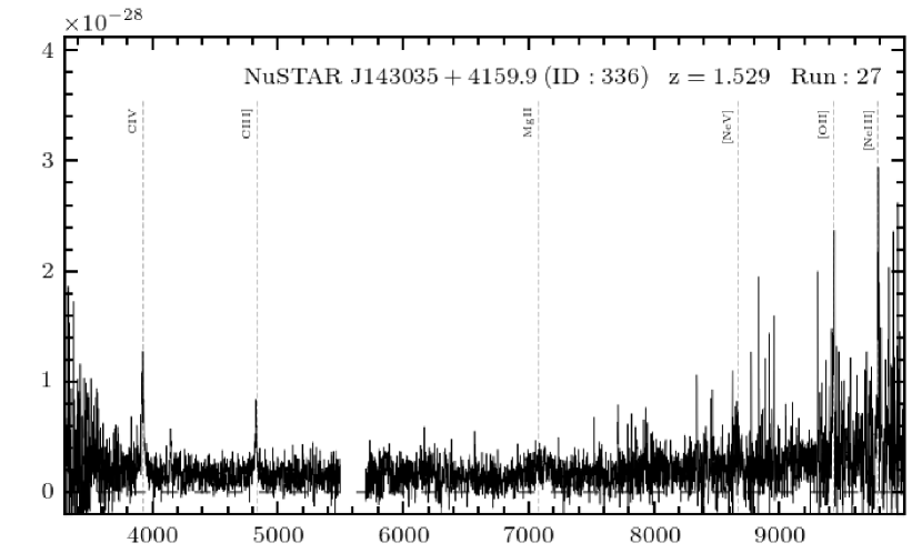
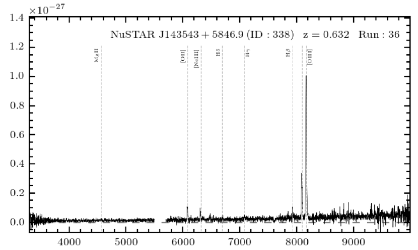
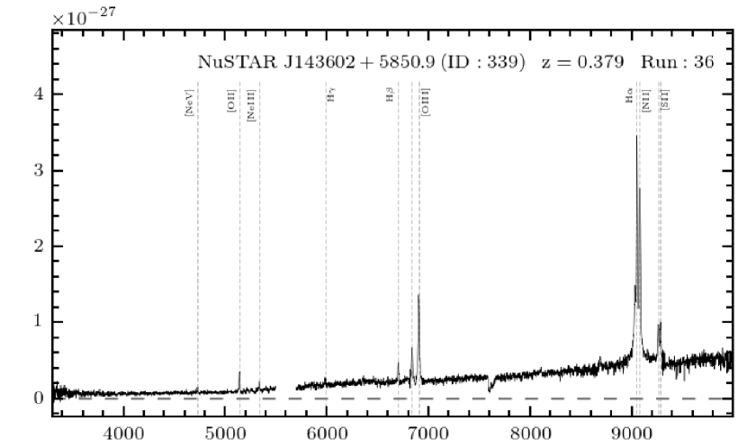
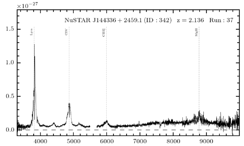
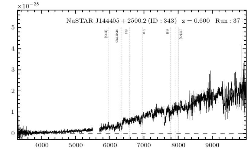
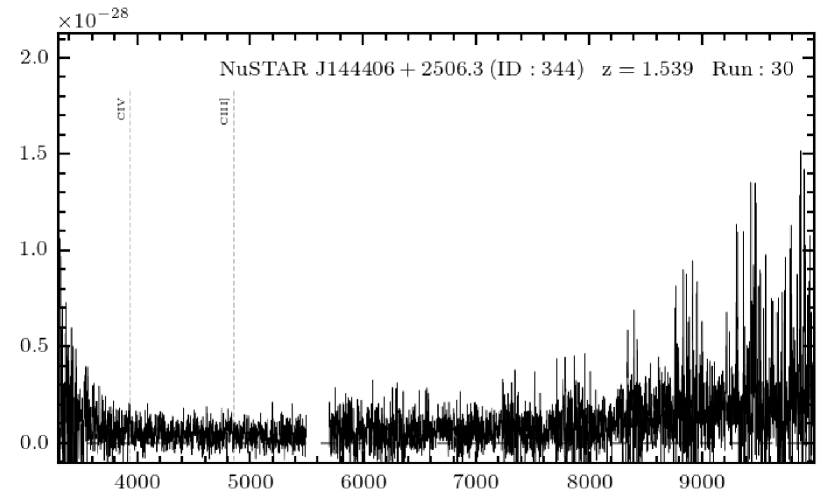
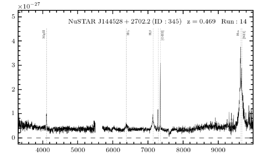
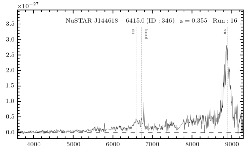
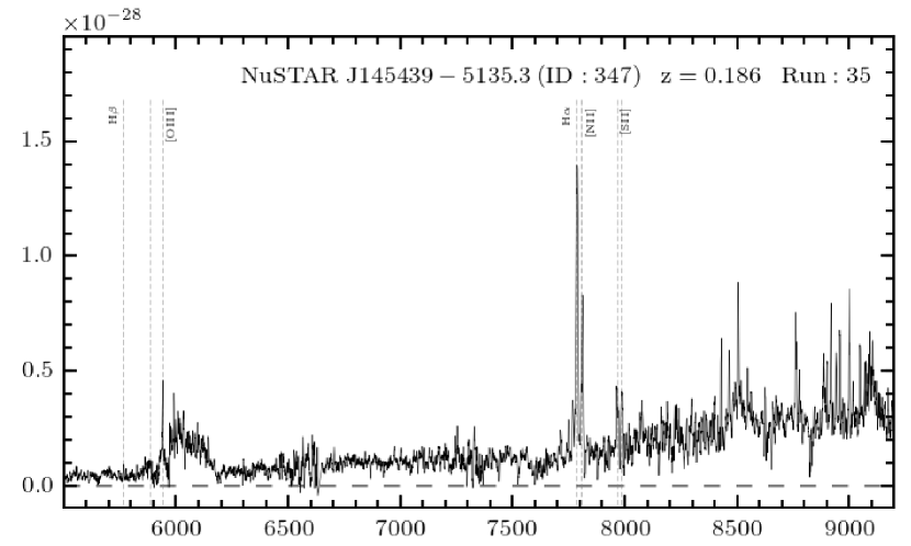
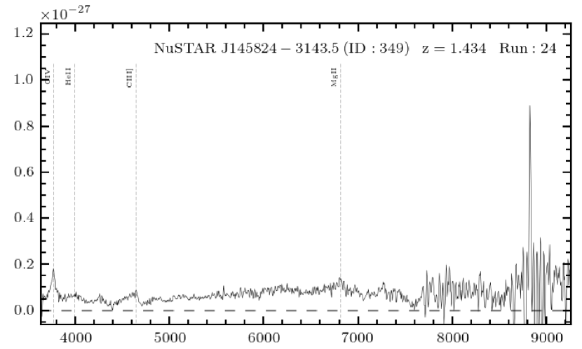
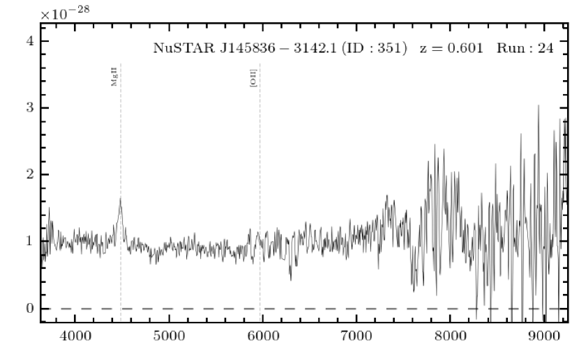
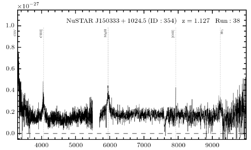
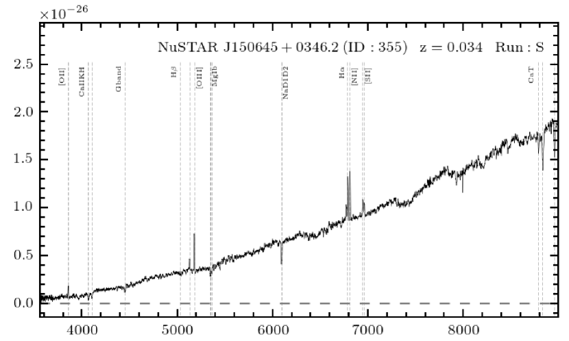
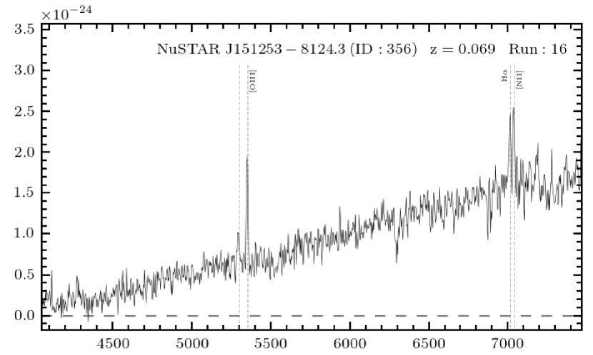
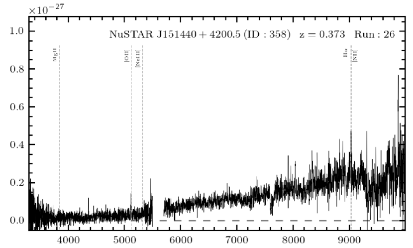
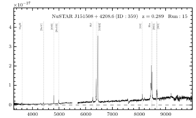
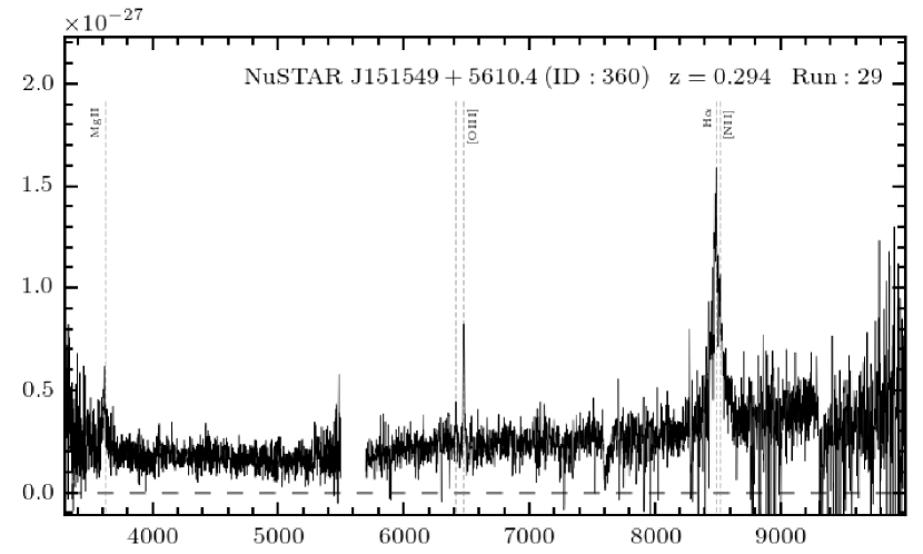
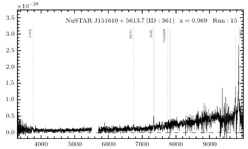
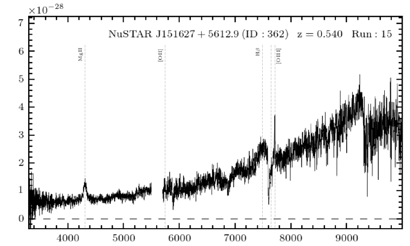
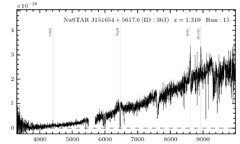
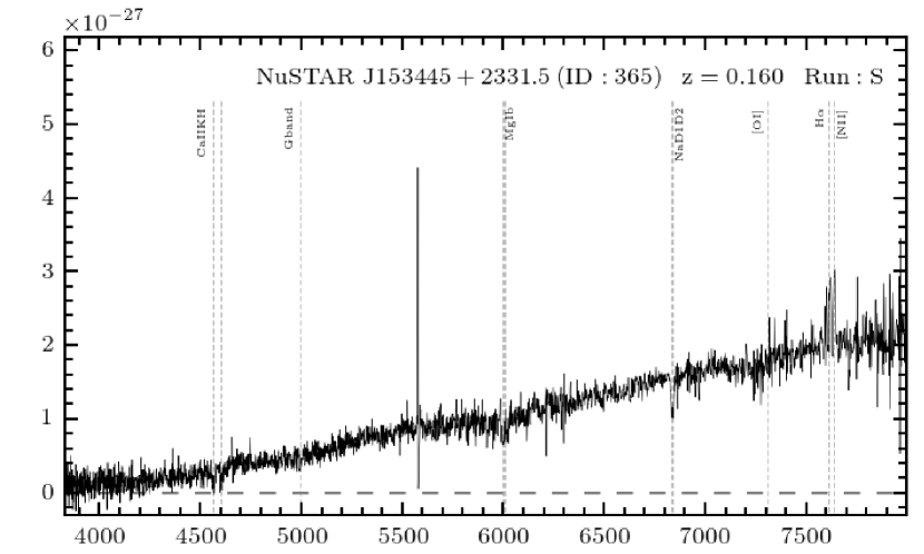
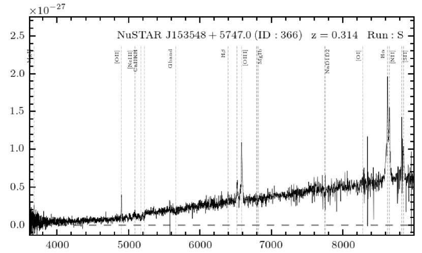
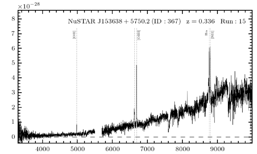
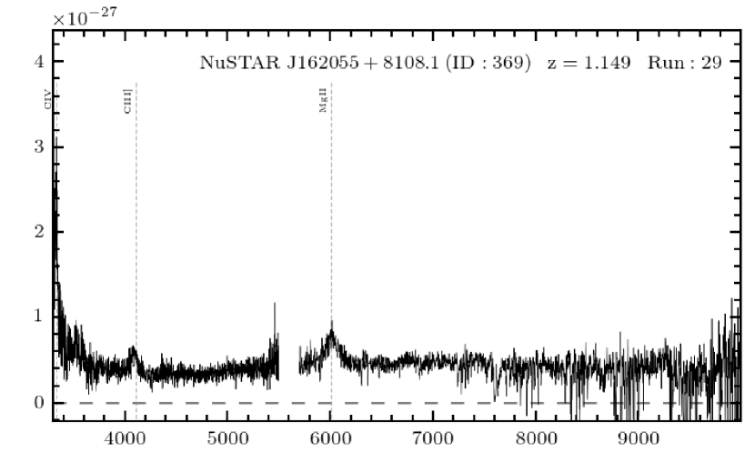
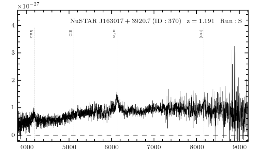
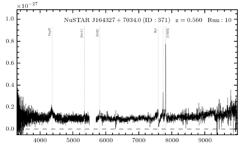
Figure 21.— Continued.

Figure 21.— Continued.

Figure 21.— Continued.

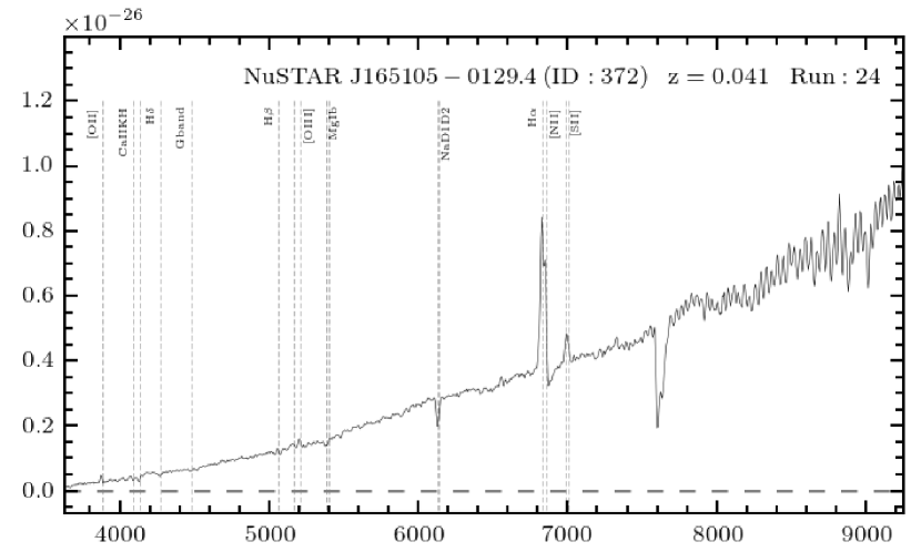
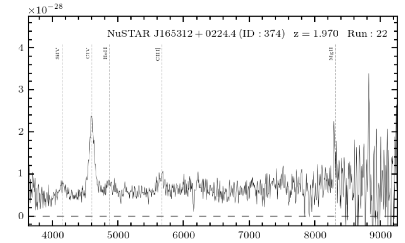
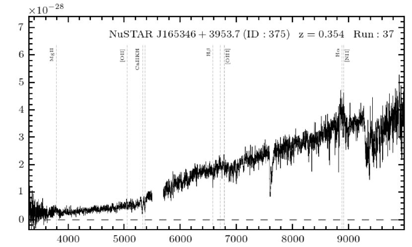
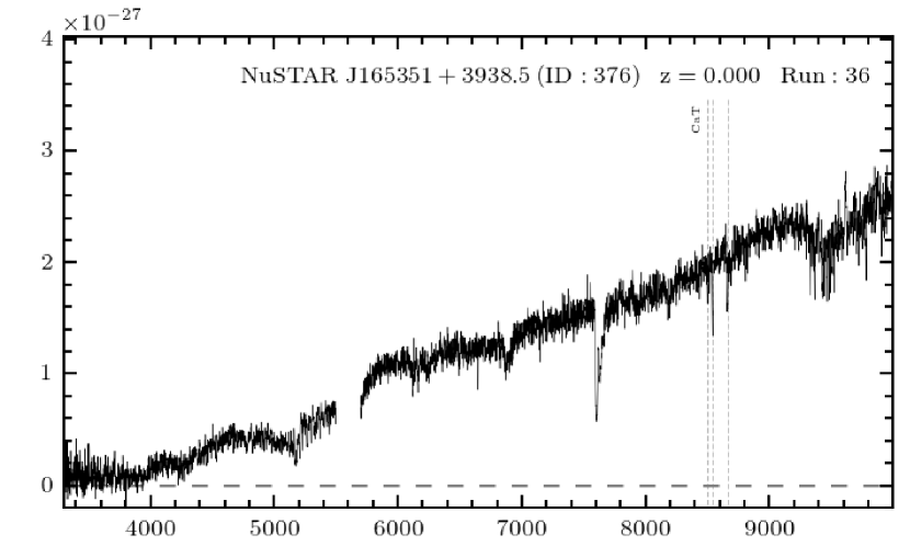
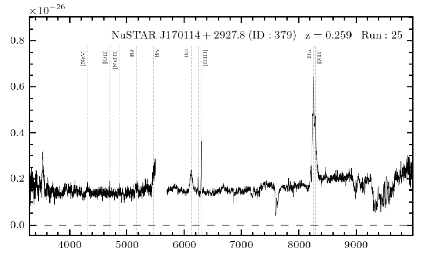
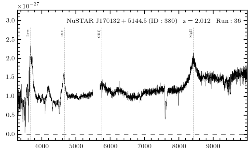
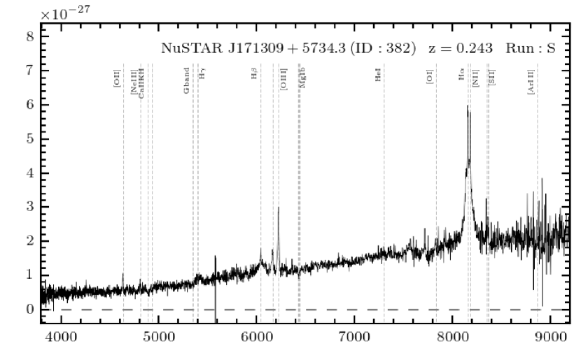
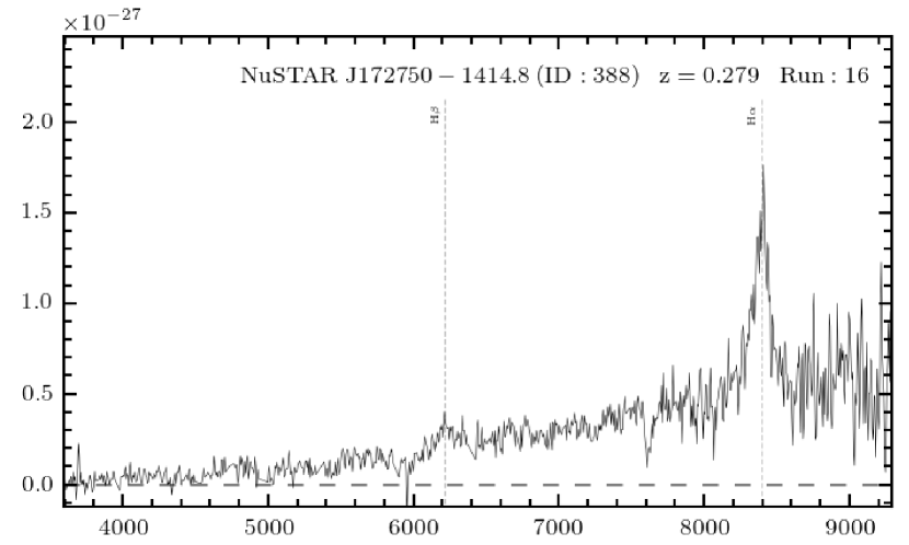
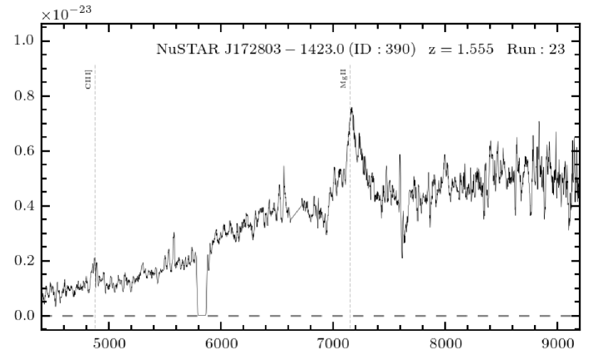
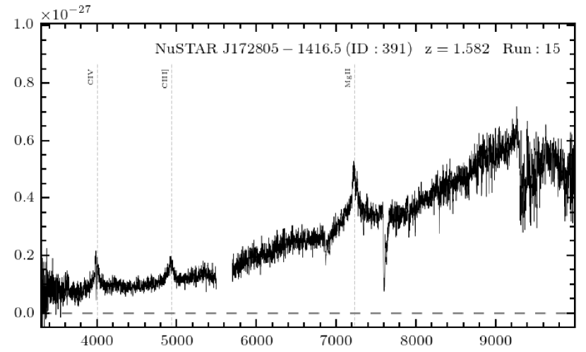
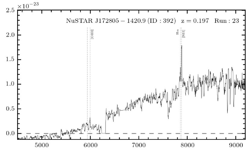
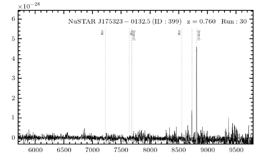
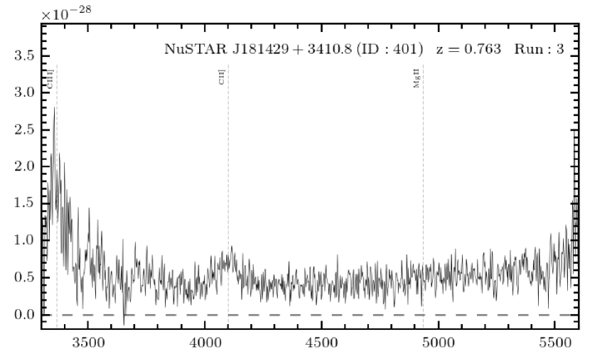
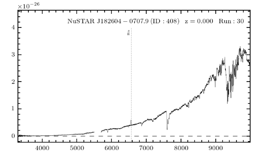
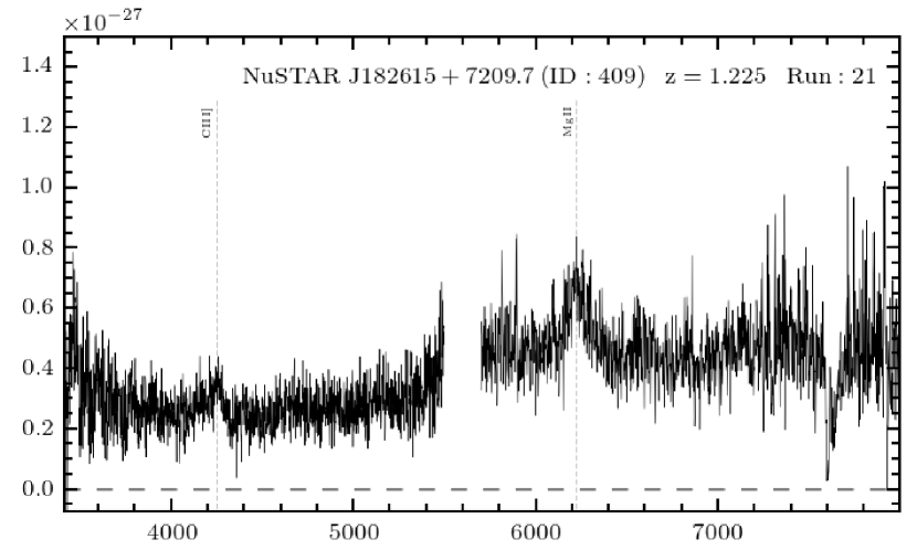
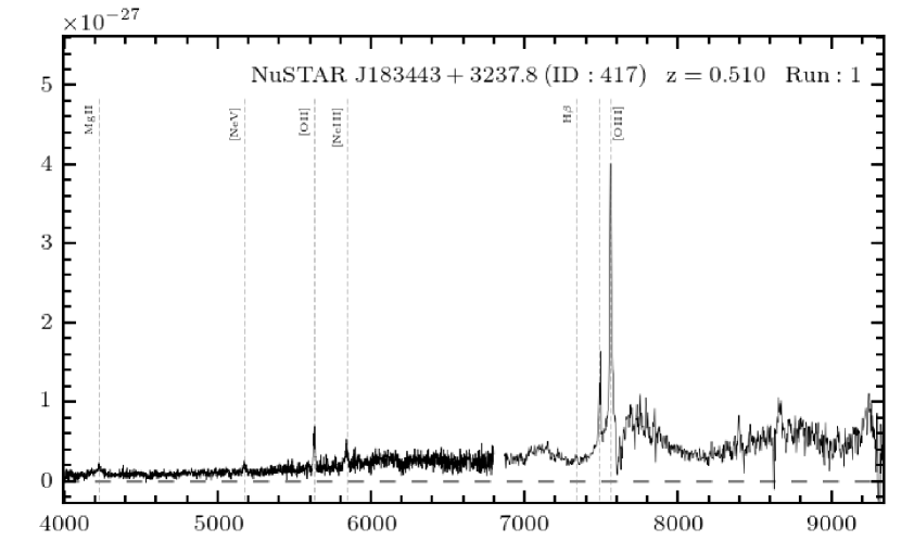
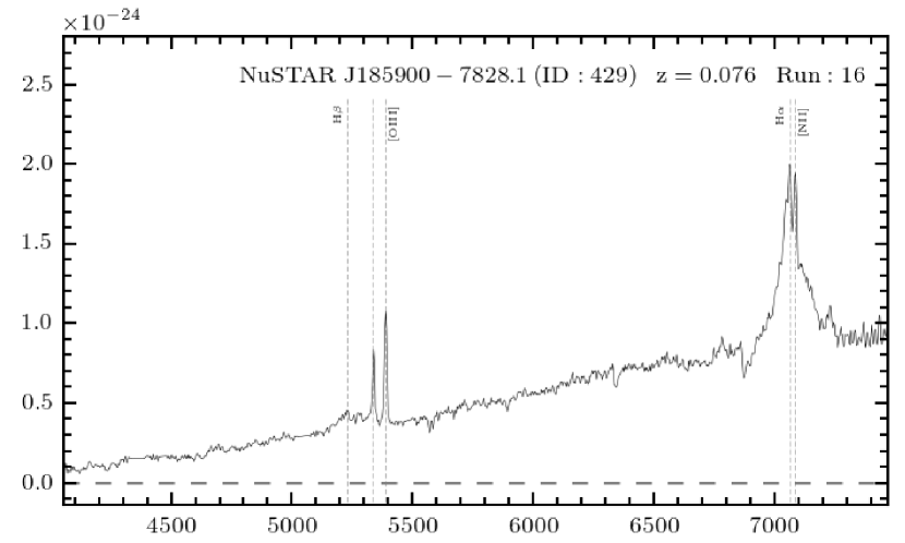
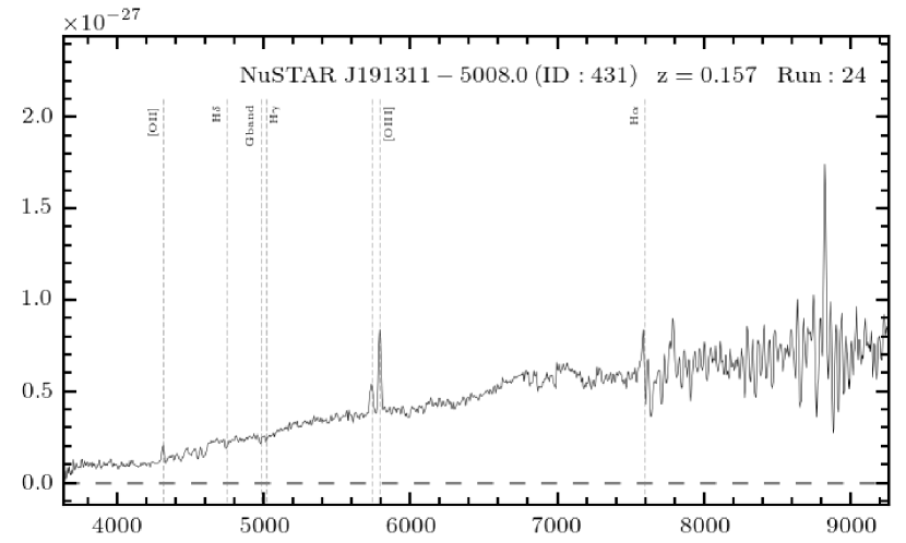
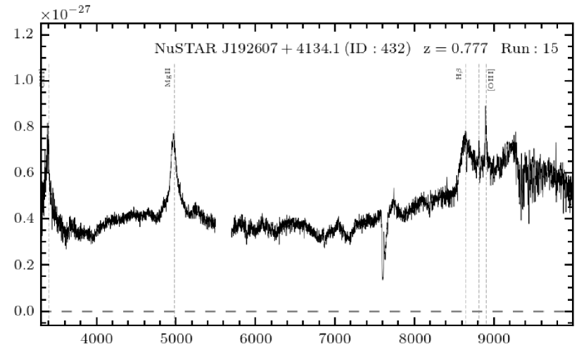
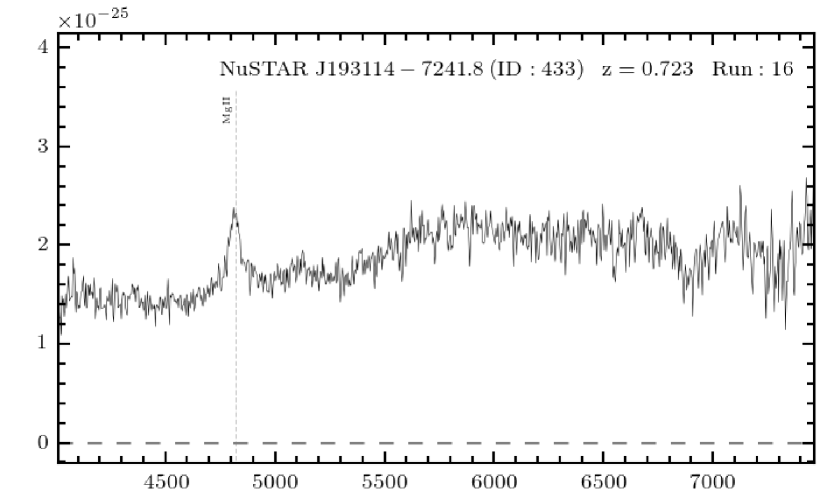
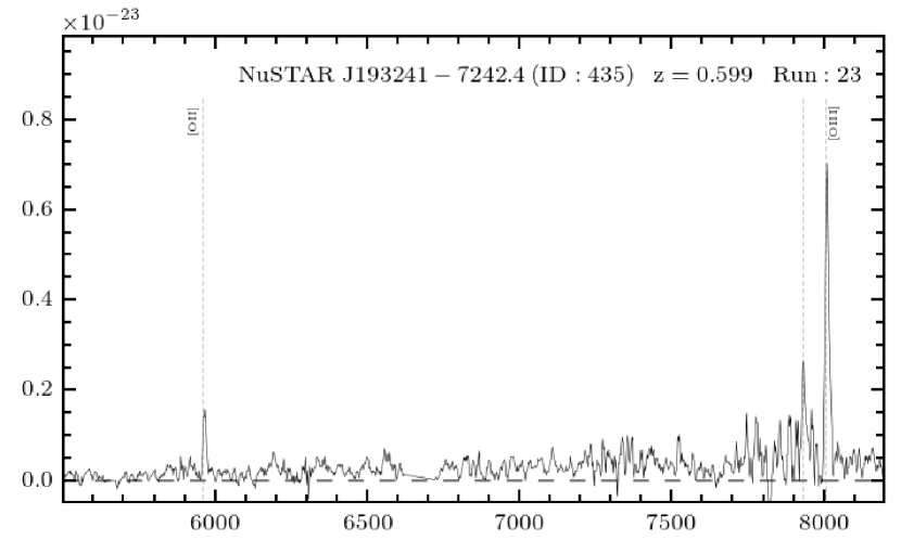
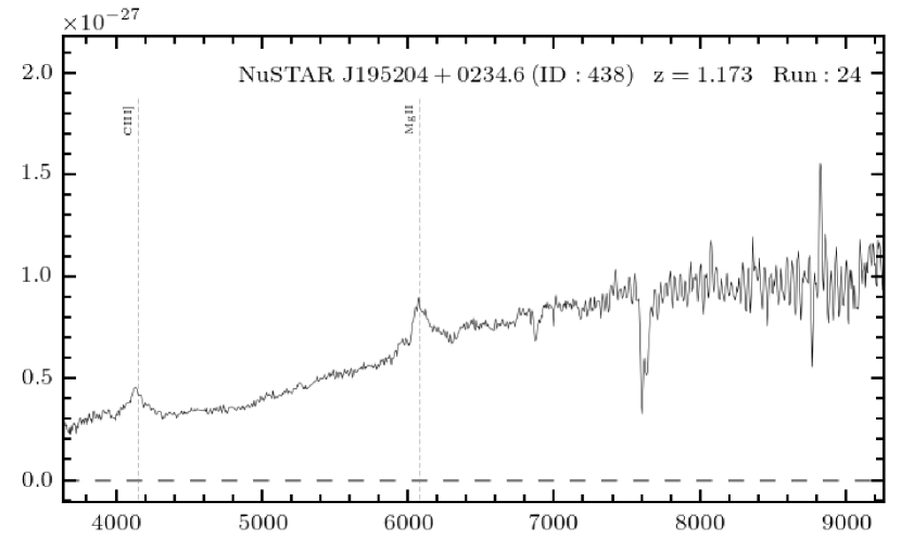
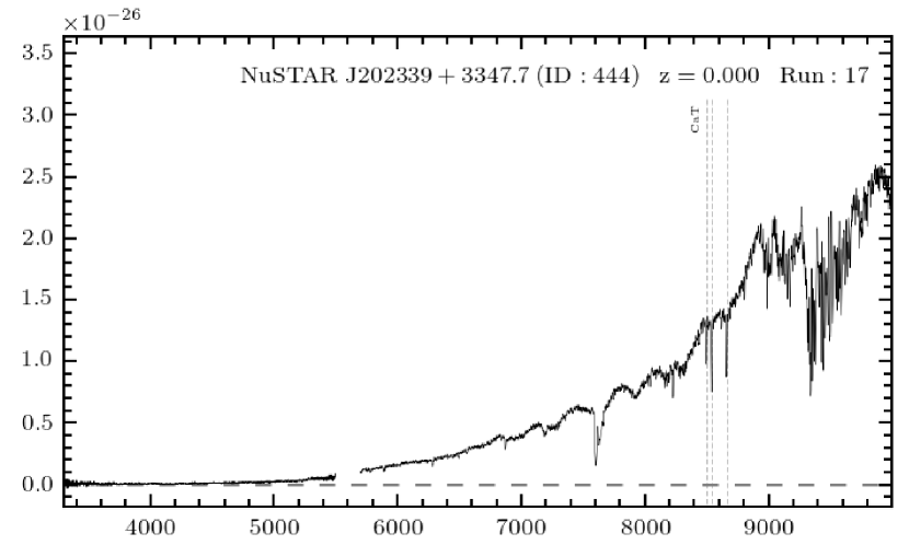
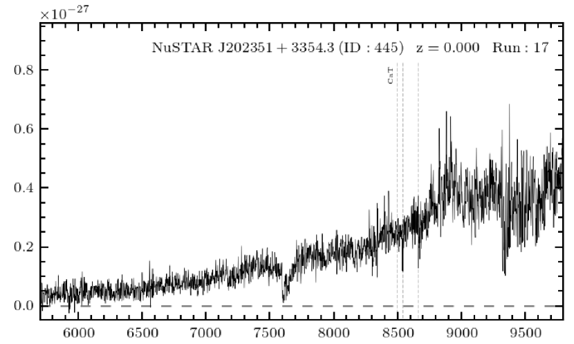
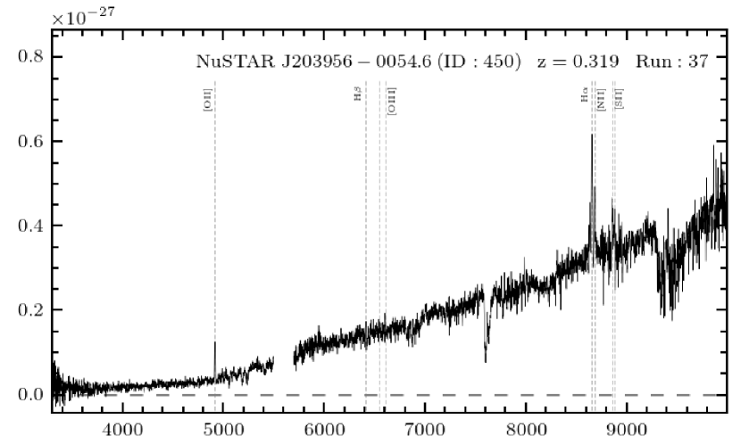
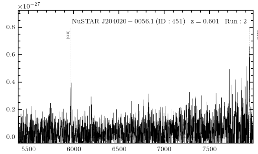
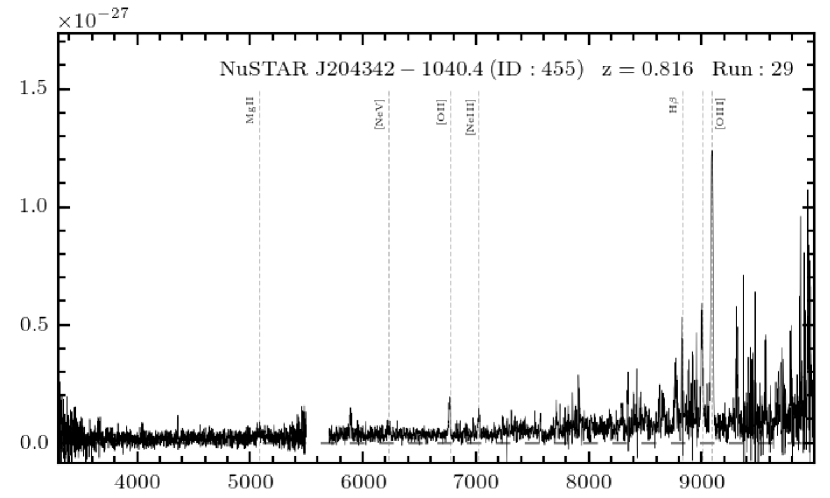
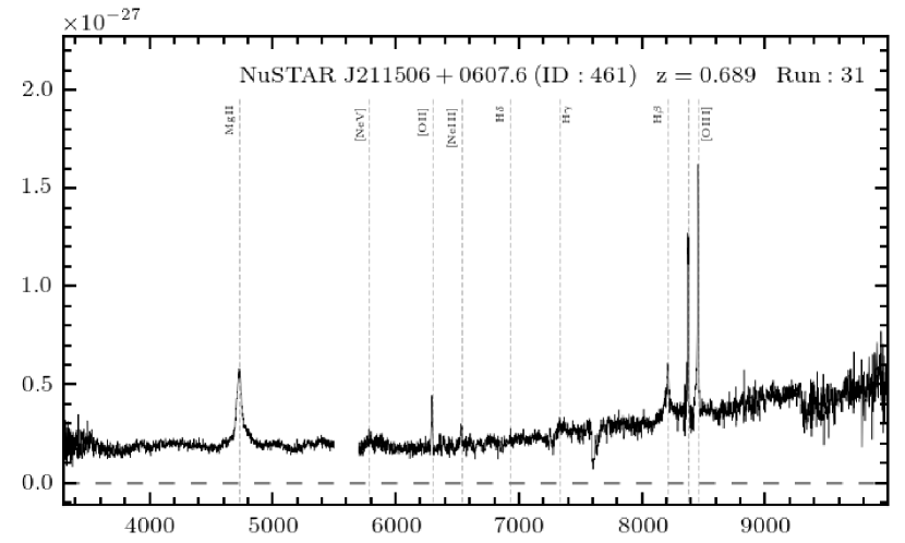
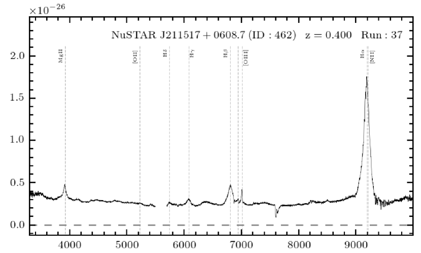
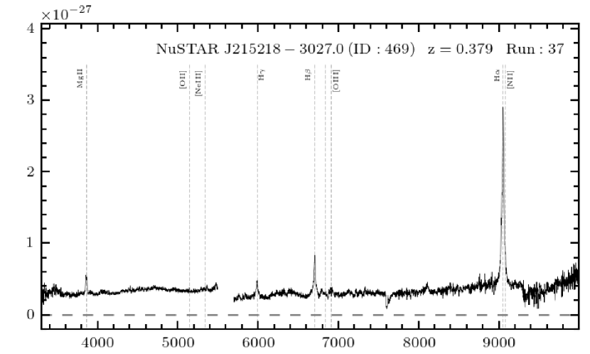
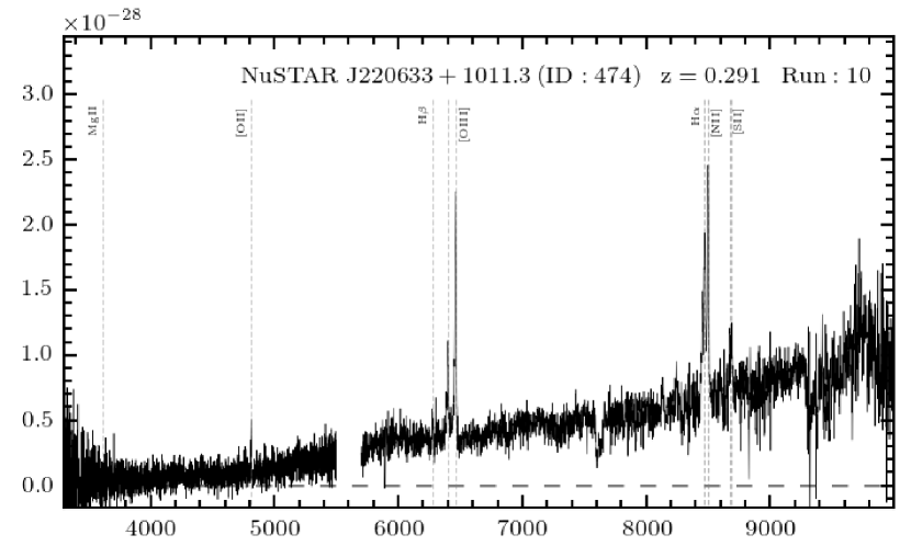
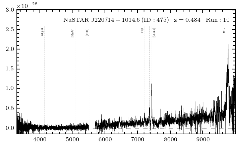
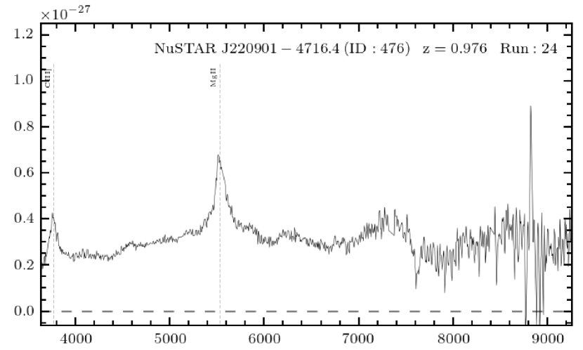
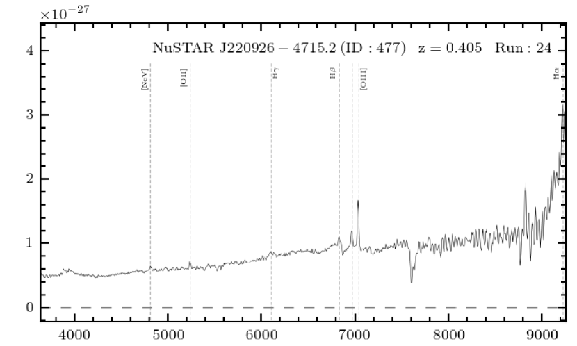
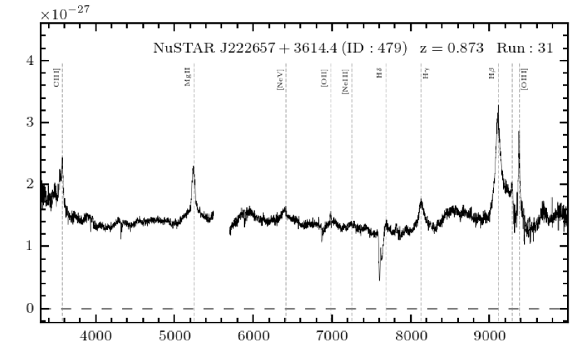
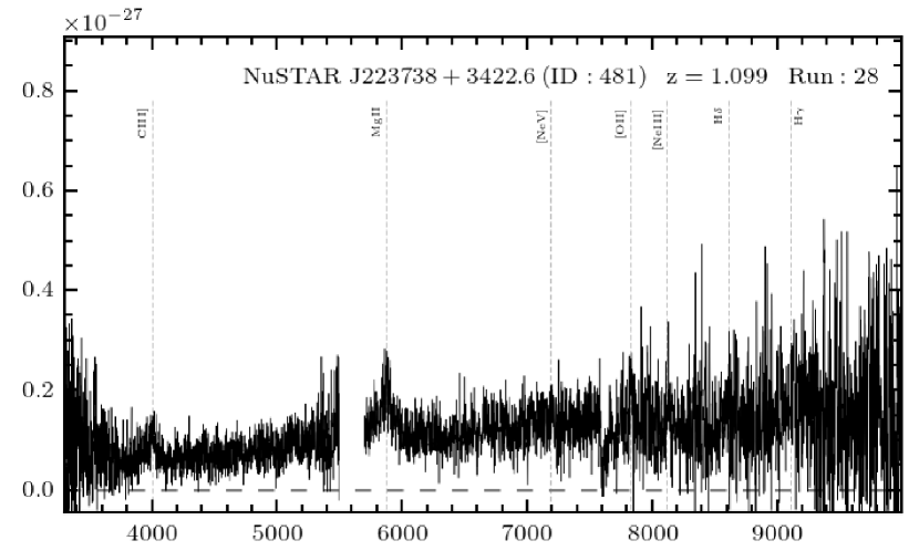
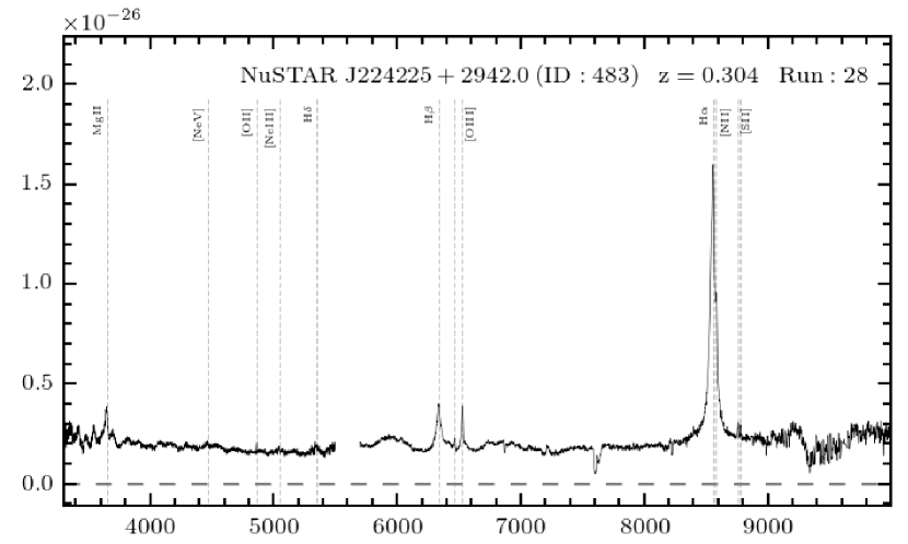
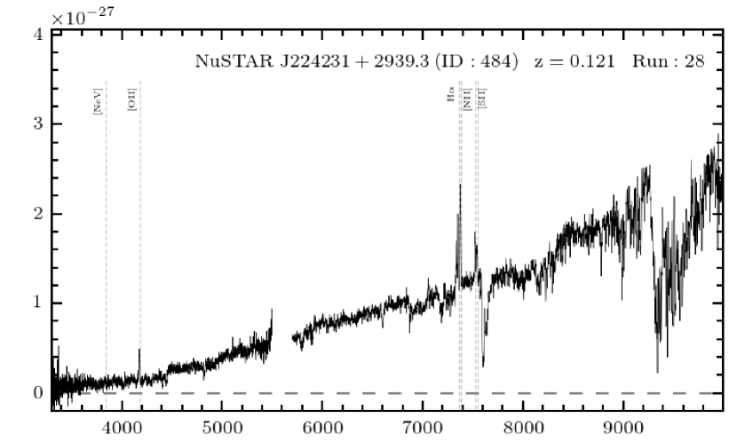
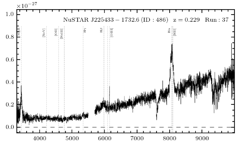
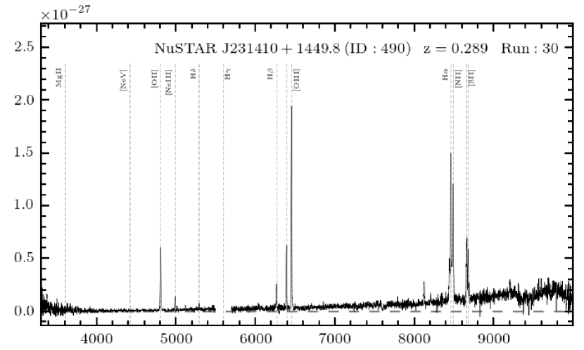
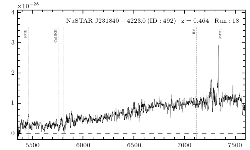
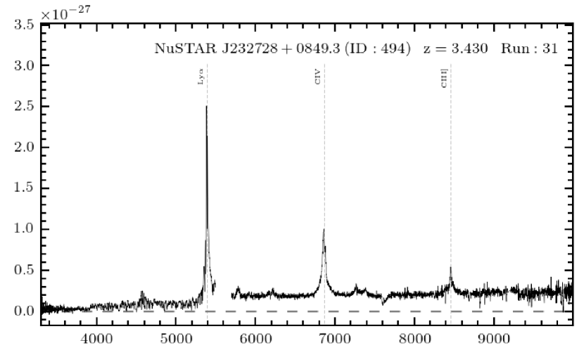
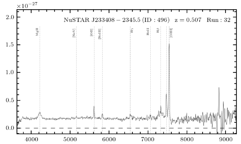
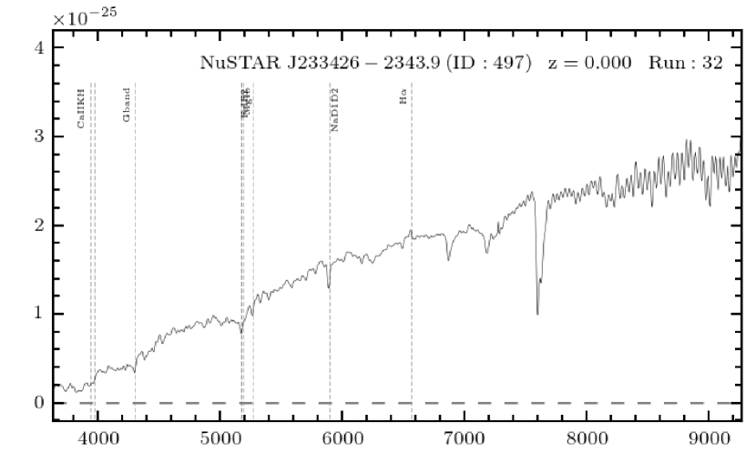
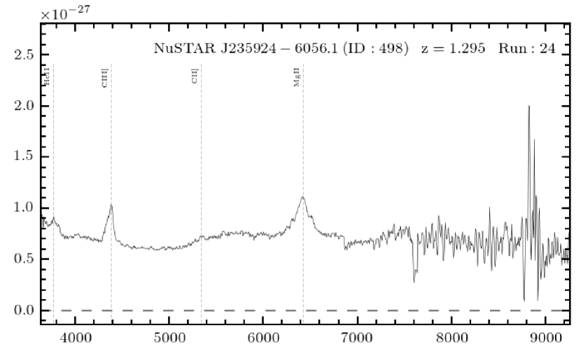
Figure 21.— Continued.

Figure 21.— Continued.

Figure 21.— Continued.

Figure 21.— Continued.

Figure 21.— Continued.

Figure 21.— Continued.

Figure 21.— Continued.

Figure 21.— Continued.

Figure 21.— Continued.

Figure 21.— Continued.

Appendix C A.3. Assessment of spurious optical and IR counterpart matches

Figure 22 shows histograms of the radial offsets between soft X-ray counterpart (Chandra, Swift XRT, and XMM-Newton) positions and the optical (SDSS and USNOB1) and IR (WISE) matches. We compare to the radial offset distributions expected for spurious matches, given the sky density of sources in the IR and optical surveys, in order to estimate spurious matching fractions.

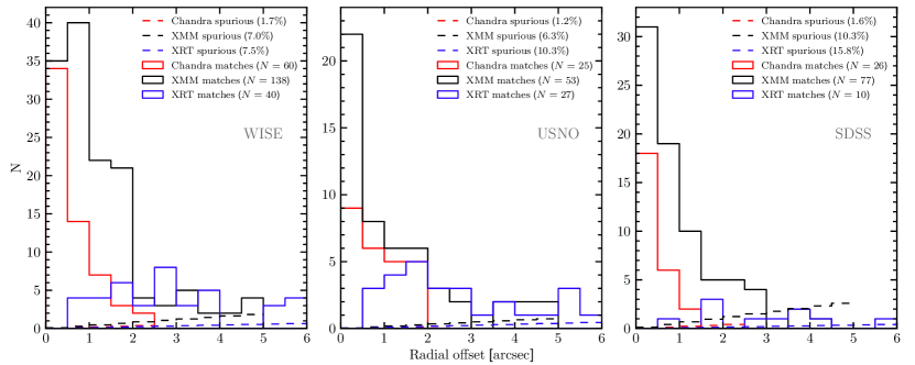
Figure 22.— Histograms showing the distributions of positional offsets between the soft X-ray (Chandra, XMM-Newton, and Swift XRT; red, black, and blue solid lines, respectively) positions and the matched WISE (left panel), USNOB1 (middle panel), and SDSS (right panel) counterparts, for the NuSTAR serendipitous survey sources with $|b|>10$^∘. The dashed lines show the distributions expected for spurious matches (i.e., assuming there are no true IR or optical counterparts to the X-ray sources); these are calculated using the IR and optical source densities, taking median values across the range of sky positions for the NuSTAR serendipitous survey sources: $3.2$ $\mathrm{arcmin}^{-2}$ for WISE; $3.3$ $\mathrm{arcmin}^{-2}$ for USNOB1; and $8.1$ $\mathrm{arcmin}^{-2}$ for SDSS. The bracketed percentages show the inferred spurious fraction (i.e., the fraction of the X-ray sources with false IR or optical matches) for each subsample.

Appendix D A.4. Assessment of spectroscopic completeness for the Type 2 fraction subsample

Here we assess the effective spectroscopic completeness of the subset of the NuSTAR serendipitous survey sample used to measure the Type 2 fraction (see Section 4.2.2). The subset is limited to hard band ($8$–$24$ keV) selected sources at redshifts of $0.1<z<0.5$ and luminosities of $2\times 10^{43}<L_{\rm 10-40keV}<2\times 10^{44}$ erg s^-1, and includes $30$ spectroscopically identified sources (all NLAGNs or BLAGNs). To assess the completeness, we must also consider the unidentified sources which may or may not lie within these redshift and luminosity ranges (i.e., sources labeled as crosses in Figure 14), and their reasons for lacking successful spectroscopic followup. Since the majority of the spectroscopically identified sources in this subsample lie at $R<20$, we consider all unidentified sources with $R<20$ (we conservatively include sources with lower limits in $R$) as potentially lying within the redshift and luminosity ranges stated above. There are $10$ such unidentified sources in total. This includes one likely BL Lac type object which we exclude due to the possibility of beaming. A further four of the unidentified sources can be safely excluded without biasing the Type 2 fraction measurement: one of these has an unambiguous optical counterpart, and simply has not yet been targetted with ground-based facilities; two have not been targetted due to the lack of Chandra or XMM-Newton coverage, required to distinguish between multiple optical counterparts within the large NuSTAR positional error circle; and for one obtaining spectroscopy is problematic due to the close proximity of brighter optical sources. There are five remaining unidentified sources to consider, where followup has not been performed due to the lack of a detection in the available Chandra and/or XMM-Newton coverage (and therefore the lack of an accurate X-ray position). Four of these have high $P_{\rm False}$ values at $8$–$24$ keV ($\log P_{\rm False}=-6.5$ to $-6.0$; i.e., close to our detection threshold of $\log P_{\rm False}=-6.0$) and comparably deep Chandra or XMM-Newton coverage, which indicates that they are likely to be spurious sources. The remaining single source is strongly detected at $8$–$24$ keV ($\log P_{\rm False}=-9.6$), and has relatively low quality Chandra and XMM-Newton coverage, so is consistent with being a genuine astrophysical source. We therefore consider the effective spectroscopic completeness of this subsample to be $97$–$100\%$ (i.e., $30/31$ or $30/30$, depending on whether the final source lies above or below $R=20$, since there is only a lower limit in $R$).

Appendix E A.5. J0650– A low $L_{\rm X}/L_{\rm MIR}$, likely X-ray weak NLSy1

Here we consider an outlier in X-ray to MIR luminosity ratio, NuSTAR J065003+6046.8 (hereafter J0650; $z=0.319$). For this source, the upper limit of $L_{\rm 10-40keV}/L_{\rm 6\mu m}<0.05$ lies below the CT AGN threshold (as shown in Figure 20). In other words, the hard X-ray luminosity is very weak compared to that expected based on the MIR luminosity ($L_{\rm 6\mu m}=3.7\times 10^{44}$ erg s^-1). The source is not detected in the full and hard NuSTAR bands, but is weakly detected in the soft band ($\log P_{\rm False}=-6.9$; $\approx 25$ net source counts, for an effective exposure time of $16$ ks), suggesting a relatively steep spectral slope. The properties of the counterparts at X-ray, IR, and optical wavelengths (see below) add confidence that the NuSTAR detection is not spurious. J0650 has a strongly detected XMM-Newton counterpart, the $0.5$–$10$ keV spectrum of which has $107$ net source counts (for an $8$ ks exposure). A power law fit provides a statistically acceptable fit to the XMM-Newton spectrum ($C/n=139/159$), and the photon index is constrained to be $\Gamma_{\rm eff}=3.1\pm 0.6$, which is very steep and above the typical range observed for AGNs. For the $3$–$10$ keV band, where NuSTAR and XMM-Newton overlap in sensitivity, the source is undetected with XMM-Newton, with $<19.5$ EPIC counts overall and a $3$–$8$ keV flux upper limit of $<1.5\times 10^{-14}$ erg s^-1 cm^-2 ($99\%$ CL). This is significantly lower than our photometric NuSTAR flux of $4.8\pm 1.6\times 10^{-14}$ erg s^-1 cm^-2 in the $3$–$8$ keV band. The disagreement could in part result from X-ray variability (between the 2003 XMM-Newton observation and the 2014 NuSTAR observation), which is especially likely in this case given the NLSy1 optical classification (see below). The NuSTAR flux is also likely boosted by the Eddington bias, which we have established to be significant at this low $3$–$8$ keV flux level (see Figure 5, and C15).

The X-ray luminosities measured at high and low energies are $L_{\mathrm{10-40\ keV}}^{\rm obs}<2.0\times 10^{43}$ erg s^-1 (from NuSTAR photometry) and $L_{\mathrm{2-10\ keV}}^{\rm obs}=2.6\times 10^{42}$ erg s^-1 (from the XMM-Newton spectrum), respectively. Given the AGN $6$ $\mu$m luminosity measured from WISE photometry ($L_{\rm 6\mu m}=3.7\times 10^{44}$ erg s^-1; the source is AGN-dominated at this wavelength based on the WISE colors), these suggest comparatively low X-ray to MIR luminosity ratios, with the $2$–$10$ keV and $10$–$40$ keV X-ray luminosities potentially suppressed by factors of $\approx 50$ and $\gtrsim 7$, respectively, with respect to the intrinsic relations for AGNs (see Figure 20). In the case of the $2$–$10$ keV luminosity, the low value is in part due to the relatively steep soft X-ray spectral slope. If the apparent X-ray suppression were due to AGN absorption we would expect a flat X-ray spectral slope ($\Gamma_{\rm eff}<1$), but the observed spectral slope is comparatively steep ($\Gamma_{\rm eff}\approx 3$). One possibility is that the source is an intrinsically X-ray weak, unobscured AGN. As described below, the source shows the properties of a NLSy1 in the optical, and intrinsic X-ray weakness has been identified for some objects in this class (e.g., Miniutti et al. 2012; Leighly et al. 2007b, a).

Further evidence for the presence of an AGN in J0650 is given by the WISE colors, which place it firmly within the MIR AGN selection regions ($W{\rm 1}$–$W{\rm 2}=1.2$; $W{\rm 2}$–$W{\rm 3}=3.2$). The source is also comparatively bright in the longer wavelength WISE bands ($W{\rm 3}=9.50\pm 0.03$ and $W{\rm 4}=7.24\pm 0.07$). On the basis of our results for WISE colors as a function of X-ray luminosity (Section 4.3.1) J0650 is statistically highly likely to have an intrinsic X-ray luminosity of $L_{\mathrm{10-40\ keV}}^{\rm int}>10^{44}$ erg s^-1. The fact that the observed X-ray luminosity is so much lower may be explained by a combination of intrinsic X-ray weakness and the steep spectral slope at low energies, the latter of which may result in a relative increase in the dust-heating photons which are reprocessed into the MIR waveband.

Key information for this object is provided by our Keck spectrum, which reveals a likely NLSy1 AGN. We detect multiple strong emission lines, from Mg II at the blue end to H$\mathrm{\alpha}$ and [N II] at the red end. The source satisfies the conventional NLSy1 definition, with a relatively narrow H$\mathrm{\beta}$ line ($\mathrm{FWHM}\approx 1710$ km s^-1), and a low [O III] $\lambda$5007$/$H$\mathrm{\beta}$ flux ratio (e.g., Goodrich, 1989). There are also multiple strong Fe II emission lines, another characteristic feature of NLSy1s (e.g., Zhou et al., 2006). Notably, the [O III] $\lambda$5007 line is contaminated by strong Fe emission. NLSy1s are associated with low black hole masses and high accretion rates (e.g., Pounds et al., 1995; Boller et al., 1996; Mathur, 2000), and typically have significantly steeper X-ray spectral slopes than normal unobscured AGNs (e.g., Boller et al., 1996; Brandt et al., 1997). The latter property is congruous with our measurement of an extremely steep X-ray photon index for J0650 ($\Gamma_{\rm eff}\approx 3$).

Appendix F A.6. Description of the Secondary Source Catalog

Here we provide a secondary catalog of $64$ NuSTAR sources identified using an independent source detection approach. This independent (or “secondary”) method uses $\mathtt{wavdetect}$ to search for significant emission peaks in the FPMA and FPMB data separately (see Section 2.1.1 of Alexander et al. 2013) and in the combined A+B data. The method was developed alongside the primary one (Section 2.3 of this paper) in order to investigate the optimum source detection methodologies for NuSTAR, and to identify sources in regions of the NuSTAR coverage which are automatically excluded in the primary source detection. We emphasise that these secondary sources are not used in any of the science analyses presented in this paper. The results in this work therefore correspond to a single, well-defined sample. Nevertheless, these secondary sources are robust NuSTAR detections, some of which will be incorporated in future NuSTAR studies (e.g., Chen et al., submitted; Tomsick et al., in prep.), and many for which ($35$ out of the $43$ sources with spectroscopic identifications) we have obtained new spectroscopic redshifts and classifications through our followup program.

The columns for the secondary source catalog are summarized in Table 7. The NuSTAR columns are equivalent to the primary catalog columns described in Section A.1, with the exception that the count rates (columns 20–25) are aperture-corrected values. The photometric columns are blank where the A+B data prohibit reliable photometric constraints. The final column assigns a character to each source, indicating the reason for not being included in the primary catalog. These are categorised into four groups: (E) the source is within or very close to the peripheral region of the NuSTAR mosaic, which is excluded from the primary source detection ($33\%$ of cases); (T) the source is narrowly offset from the central science target position for the NuSTAR observation (and thus automatically excluded; see Section 2.3), or from another bright source in the field ($11\%$); (X) the source lies in a region which is masked out, or in a NuSTAR field which is excluded, from the primary source detection ($44\%$; e.g., due to highly contaminating stray light or a bright science target); or (L) the source has a comparatively low detection significance ($12\%$).

Table 7Column Descriptions for the Secondary NuSTAR Serendipitous Source Catalog

Column number	Description
1	Unique source identification number (ID).
2	Unique NuSTAR source name.
3, 4	Right ascension (R.A.) and declination (decl.).
5–16	Total, background, and net source counts for the three standard energy bands, and associated errors.
17–19	Net vignetting-corrected exposure times at the source position, for the combined A+B data.
20–25	Net source count rates for the three standard energy bands, and associated errors.
26–31	Fluxes in the three standard bands and associated errors.
32–34	Observatory name and coordinates (R.A. and decl.) for the lower-energy X-ray counterpart.
35–37	Reference and coordinates (R.A. and decl.) for the optical or WISE counterpart.
38	Spectroscopic redshift.
39	Non-absorption-corrected, rest-frame $10$–$40$ keV luminosity.
40	Character indicating the reason for not appearing in the primary catalog.

Notes. The full catalog is available as a machine readable electronic table.

In Table 8 we tabulate details of the optical spectroscopic properties of individual sources from the secondary catalog with spectroscopic coverage. The columns are equivalent to those in Table LABEL:specTable, with the exception of an additional observing run label (“G”) to mark sources followed up with Gemini-South in January and February of 2016. For $78\%$ of the sources in Table 8 the spectroscopic constraints are from our dedicated followup program (with Keck, Palomar, NTT, Magellan, and Gemini), and for $22\%$ they are from the SDSS or the literature. Individual source spectra ($F_{\mathrm{\nu}}$ versus $\lambda$) are shown in Figure 23.

Table 8Summary of the optical spectroscopy for the secondary catalog sources.

ID	NuSTAR Name	$z$	Type	Lines	Notes	Run
(1)	(2)	(3)	(4)	(5)	(6)	(7)
1	NuSTARJ001639+8139.8	0.000	Gal	$\cdot$$\cdot$$\cdot$	Bright star	28
3	NuSTARJ001844-1022.6	0.076	NL	[O II] Ca${}_{\mathrm{H,K}}^{\mathrm{\dagger}}$ G-band† H$\mathrm{\beta}^{\mathrm{\dagger}}$ Mg Ib† Na${}_{\mathrm{D1,D2}}^{\mathrm{\dagger}}$ H$\mathrm{\alpha}$ [N II] [S II]	$\cdot$$\cdot$$\cdot$	S
4	NuSTARJ011018-4612.1	$\cdot$$\cdot$$\cdot$	$\cdot$$\cdot$$\cdot$	$\cdot$$\cdot$$\cdot$	Continuum detected	11
5	NuSTARJ011053-4602.6	0.626	NL	[O II] H$\mathrm{\gamma}$ H$\mathrm{\beta}$ [O III]	$\cdot$$\cdot$$\cdot$	18
6	NuSTARJ022801+3115.9	1.857	BL	Ly$\mathrm{\alpha}$ C IV C III] Mg II	$\cdot$$\cdot$$\cdot$	31
7	NuSTARJ023448-2936.6	0.313	NL	H$\mathrm{\beta}$ [O III] H$\mathrm{\alpha}$ [N II]	$\cdot$$\cdot$$\cdot$	G
8	NuSTARJ023459-2944.6	0.446	BL	$\cdot$$\cdot$$\cdot$	Caccianiga et al. (2008)	L
9	NuSTARJ031602-0221.0	0.821	NL	[O II] H$\mathrm{\beta}$ [O III]	$\cdot$$\cdot$$\cdot$	31
10	NuSTARJ033313-3612.0	$\cdot$$\cdot$$\cdot$	$\cdot$$\cdot$$\cdot$	$\cdot$$\cdot$$\cdot$	Two possible counterparts at $z\approx 1$; Wong et al. (2008)	L
11	NuSTARJ033342-3613.9	0.559	NL	[O II] H$\mathrm{\beta}$ [O III]	$\cdot$$\cdot$$\cdot$	11
12	NuSTARJ033406-3603.9	0.910	BL	Mg II	$\cdot$$\cdot$$\cdot$	11
13	NuSTARJ034403-4441.0	0.275	NL?	Ca${}_{\mathrm{H,K}}^{\mathrm{\dagger}}$ G-band† [O III] Mg Ib† Na${}_{\mathrm{D1,D2}}^{\mathrm{\dagger}}$ [O I] H$\mathrm{\alpha}$ [N II] [S II]	$\cdot$$\cdot$$\cdot$	32
15	NuSTARJ043754-4716.0	0.337	NL	[O II] H$\mathrm{\beta}$ H$\mathrm{\alpha}$ [N II]	$\cdot$$\cdot$$\cdot$	23
17	NuSTARJ081911+7046.6	0.720	NL	[O II] H$\mathrm{\beta}$ [O III]	[O III] asymmetry	13
18	NuSTARJ090223-4039.4	0.087	BL	H$\mathrm{\beta}$ [O III] [O I] H$\mathrm{\alpha}$ [N II]	$\cdot$$\cdot$$\cdot$	11
20	NuSTARJ092418-3142.2	0.000	Gal	$\cdot$$\cdot$$\cdot$	Continuum detected	22
21	NuSTARJ094734-3104.2	$\cdot$$\cdot$$\cdot$	$\cdot$$\cdot$$\cdot$	$\cdot$$\cdot$$\cdot$	Continuum detected	24
22	NuSTARJ101600-3329.6	0.231	NL	[O II] [O III] H$\mathrm{\alpha}$ [N II]	$\cdot$$\cdot$$\cdot$	22
27	NuSTARJ105008-5958.8	0.000	Gal	H$\mathrm{\delta}$ H$\mathrm{\gamma}$ H$\mathrm{\beta}$ Na${}_{\mathrm{D1,D2}}^{\mathrm{\dagger}}$ H$\mathrm{\alpha}$	$\cdot$$\cdot$$\cdot$	11
28	NuSTARJ110445+3811.1	0.144	NL	[O II] [Ne III] Ca${}_{\mathrm{H,K}}^{\mathrm{\dagger}}$ H$\mathrm{\delta}^{\mathrm{\dagger}}$ H$\mathrm{\beta}$ [O III] Mg Ib† Na${}_{\mathrm{D1,D2}}^{\mathrm{\dagger}}$ [O I] H$\mathrm{\alpha}$ [N II] [S II]	$\cdot$$\cdot$$\cdot$	S
30	NuSTARJ120259+4430.4	0.465	NL	H$\mathrm{\beta}$ [O III]	$\cdot$$\cdot$$\cdot$	14
31	NuSTARJ120711+3348.4	0.135	BL	[O II] [Ne III] Ca${}_{\mathrm{H,K}}^{\mathrm{\dagger}}$ H$\mathrm{\gamma}$ H$\mathrm{\beta}$ [O III] H$\mathrm{\alpha}$ [N II]	$\cdot$$\cdot$$\cdot$	S
32	NuSTARJ120930-0500.1	0.391	NL	H$\mathrm{\delta}^{\mathrm{\dagger}}$ H$\mathrm{\beta}$ [O III] [O I]	$\cdot$$\cdot$$\cdot$	G
33	NuSTARJ121027+3929.1	0.615	BL Lac	Ca${}_{\mathrm{H,K}}^{\mathrm{\dagger}}$ H$\mathrm{\delta}^{\mathrm{\dagger}}$ G-band† H$\mathrm{\gamma}^{\mathrm{\dagger}}$ H$\mathrm{\beta}^{\mathrm{\dagger}}$ [O III] Mg Ib†	Morris et al. (1991)	S
34	NuSTARJ121038+3930.7	1.033	NL	C III] C II] [Ne IV] Mg II [Ne V] [O II] [Ne III] H$\mathrm{\beta}$ [O III]	$\cdot$$\cdot$$\cdot$	15
35	NuSTARJ121049+3928.5	0.023	NL	[O II] Ca${}_{\mathrm{H,K}}^{\mathrm{\dagger}}$ G-band† H$\mathrm{\gamma}$ H$\mathrm{\beta}$ [O III] Mg Ib† Na${}_{\mathrm{D1,D2}}^{\mathrm{\dagger}}$ [O I] H$\mathrm{\alpha}$ [N II] [S II] CaT†	$\cdot$$\cdot$$\cdot$	S
36	NuSTARJ121854+2958.0	0.175	NL?	[O II] [Ne III] H$\mathrm{\delta}$ H$\mathrm{\gamma}$ H$\mathrm{\beta}$ [O III] [O I] H$\mathrm{\alpha}$ [N II] [S II] [Ar III]	$\cdot$$\cdot$$\cdot$	S
37	NuSTARJ123559-3951.9	0.000	Gal	$\cdot$$\cdot$$\cdot$	Star	L
38	NuSTARJ125021+2635.9	0.751	BL	Mg II [Ne V] [O II] [Ne III] H$\mathrm{\beta}$ [O III]	$\cdot$$\cdot$$\cdot$	27
39	NuSTARJ125605+5643.8	0.984	NL	Mg II [O II] [Ne III]	$\cdot$$\cdot$$\cdot$	12
40	NuSTARJ125711+2748.1	0.306	NL	[O II] Ca${}_{\mathrm{H,K}}^{\mathrm{\dagger}}$ [O III] H$\mathrm{\alpha}$ [N II]	$\cdot$$\cdot$$\cdot$	15
41	NuSTARJ125715+2746.6	$\cdot$$\cdot$$\cdot$	$\cdot$$\cdot$$\cdot$	CaT†	Counterpart uncertainty	15
42	NuSTARJ125744+2751.2	0.325	NL	[O II] Ca${}_{\mathrm{H,K}}^{\mathrm{\dagger}}$ [O III] H$\mathrm{\alpha}$ [N II]	$\cdot$$\cdot$$\cdot$	15
43	NuSTARJ130157-6358.1	0.000	Gal	$\cdot$$\cdot$$\cdot$	Krivonos et al. (2015)	L
45	NuSTARJ130616-4930.8	0.284	BL?	H$\mathrm{\beta}$ [O III] H$\mathrm{\alpha}$ [N II]	$\cdot$$\cdot$$\cdot$	16
46	NuSTARJ134447+5554.0	0.458	BL?	Mg II H$\mathrm{\beta}$ [O III]	$\cdot$$\cdot$$\cdot$	14
48	NuSTARJ143256-4419.3	0.119	NL	Ca${}_{\mathrm{H,K}}^{\mathrm{\dagger}}$ G-band† H$\mathrm{\beta}^{\mathrm{\dagger}}$ Mg Ib† Na${}_{\mathrm{D1,D2}}^{\mathrm{\dagger}}$	Cluster ABELL 3602	24
49	NuSTARJ155520-3315.1	0.551	NL	[O II] H$\mathrm{\beta}$ [O III]	$\cdot$$\cdot$$\cdot$	23
50	NuSTARJ165050-0126.6	0.791	BL	Mg II H$\mathrm{\beta}$	$\cdot$$\cdot$$\cdot$	24
51	NuSTARJ165104-0127.2	0.852	NL	[Ne V] [O II] [Ne III] [O III]	$\cdot$$\cdot$$\cdot$	30
52	NuSTARJ170016+7840.7	0.778	BL	Mg II [O II] [O III]	$\cdot$$\cdot$$\cdot$	9
53	NuSTARJ172822-1421.4	0.688	NL	[O II] H$\mathrm{\gamma}$ H$\mathrm{\beta}$ [O III]	$\cdot$$\cdot$$\cdot$	23
55	NuSTARJ175307-0123.7	0.451	NL?	[O II] [Ne III] H$\mathrm{\beta}$ [O III]	$\cdot$$\cdot$$\cdot$	24
56	NuSTARJ181417+3411.6	0.714	BL	Mg II [Ne V] [O II] H$\mathrm{\beta}$ [O III]	$\cdot$$\cdot$$\cdot$	30
63	NuSTARJ223654+3423.4	0.148	NL	[O II] [O III] H$\mathrm{\alpha}$ [N II]	$\cdot$$\cdot$$\cdot$	31
64	NuSTARJ224037+0802.6	1.418	BL	C IV C III] Mg II [O II]	$\cdot$$\cdot$$\cdot$	30

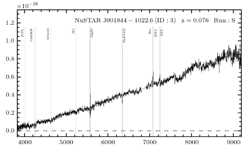
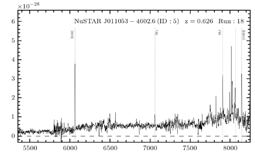
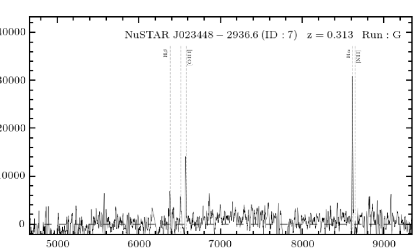
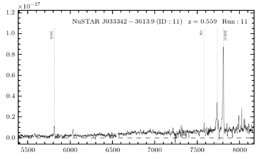
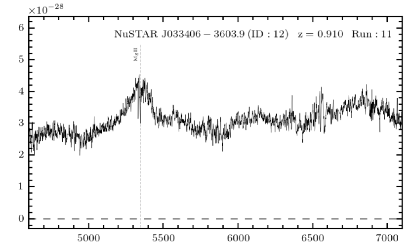
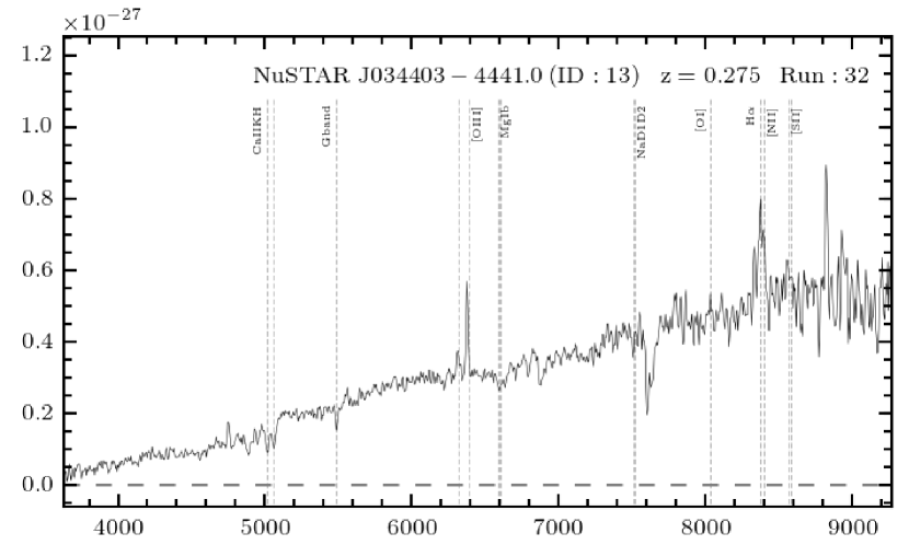
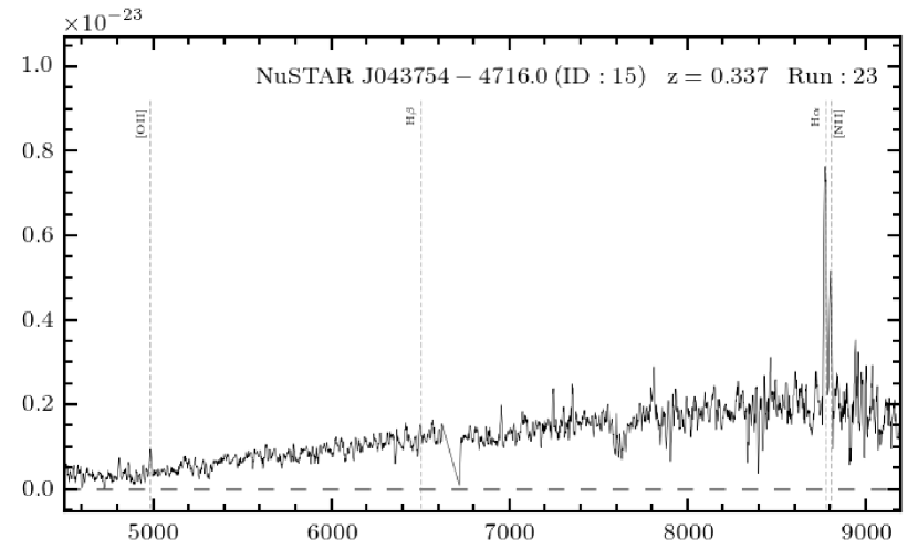
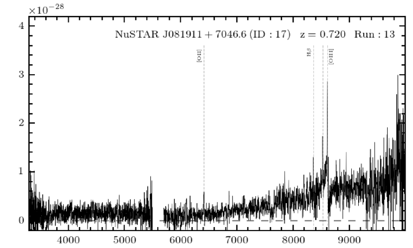
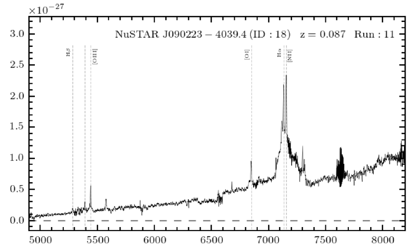
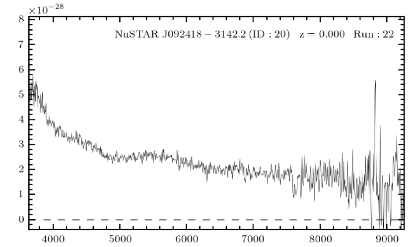
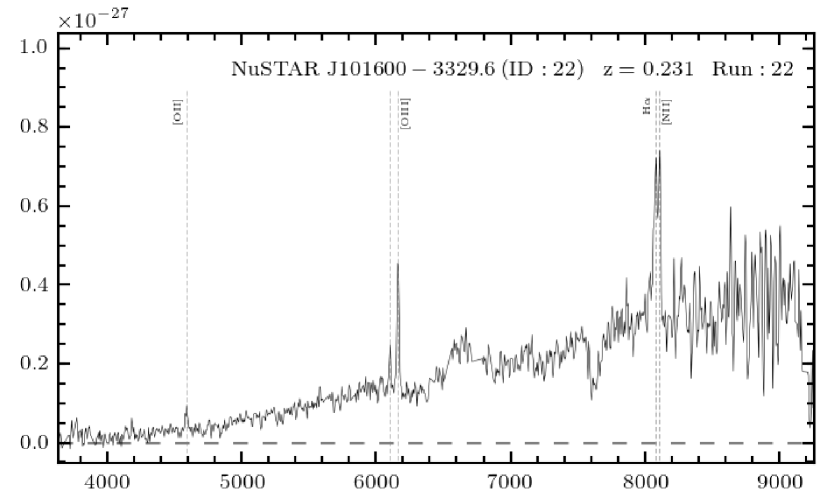
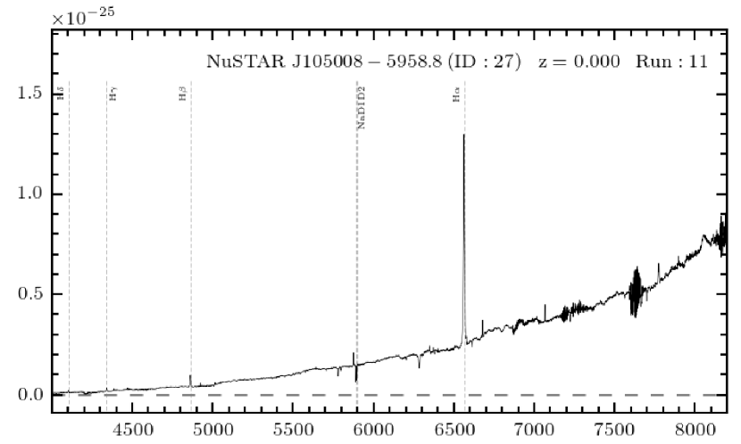
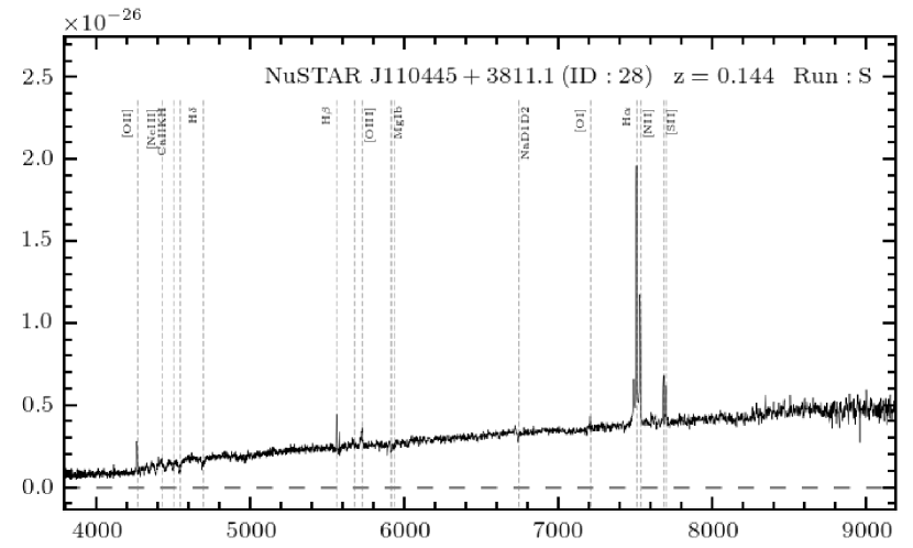
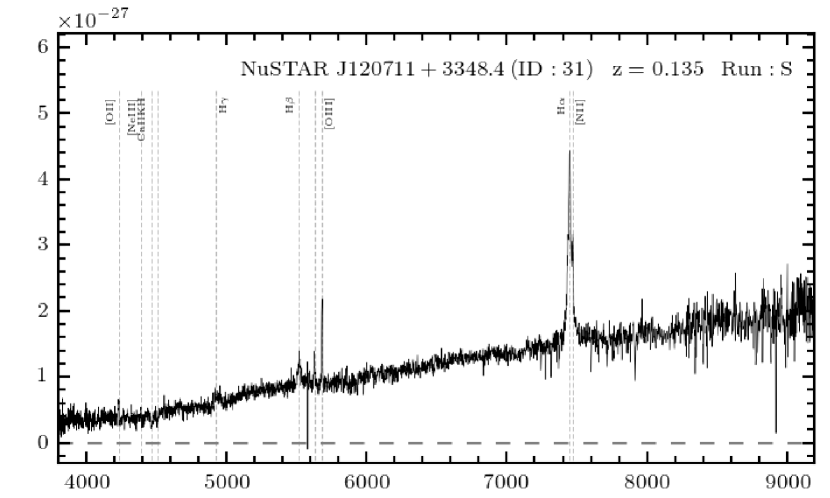
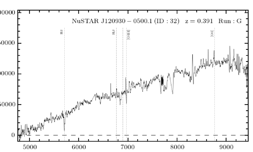
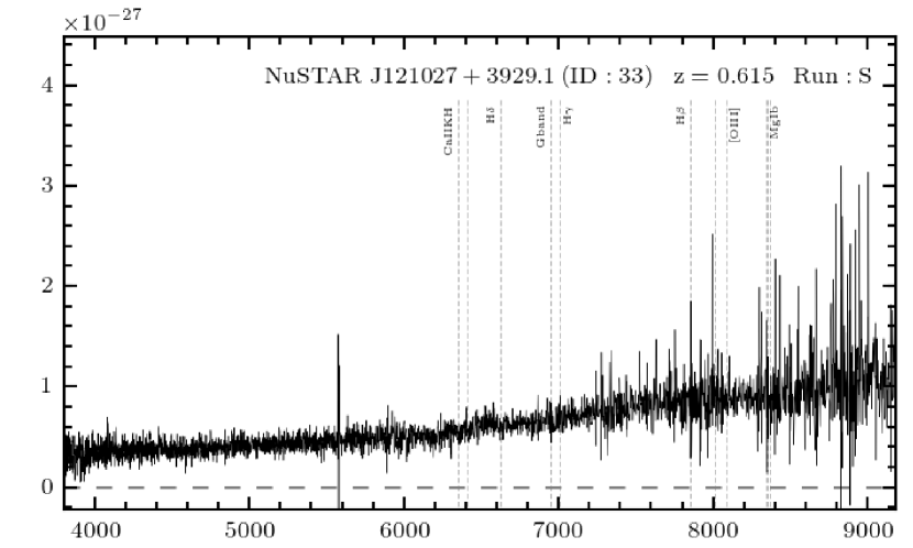
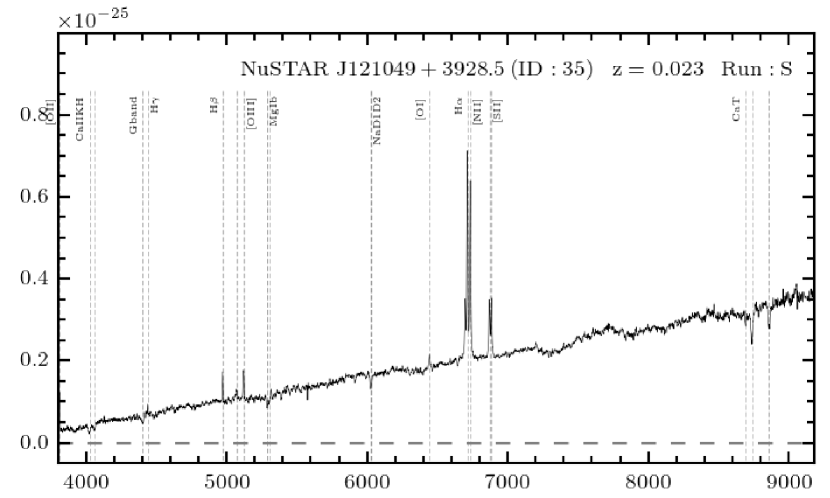
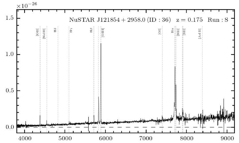
Figure 23.— Optical spectra for the secondary catalog sources (continued on the following pages). The axes and labelling are the same as for Figure 21. Full resolution figures are available online.

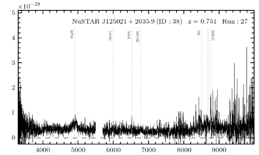
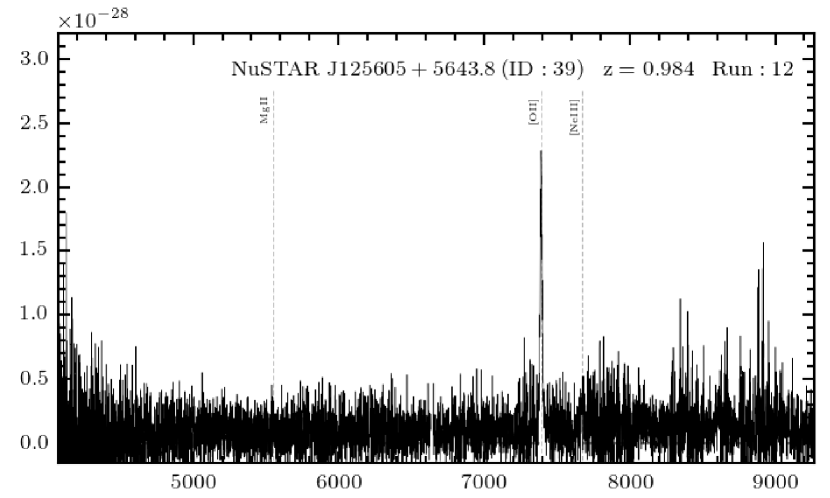
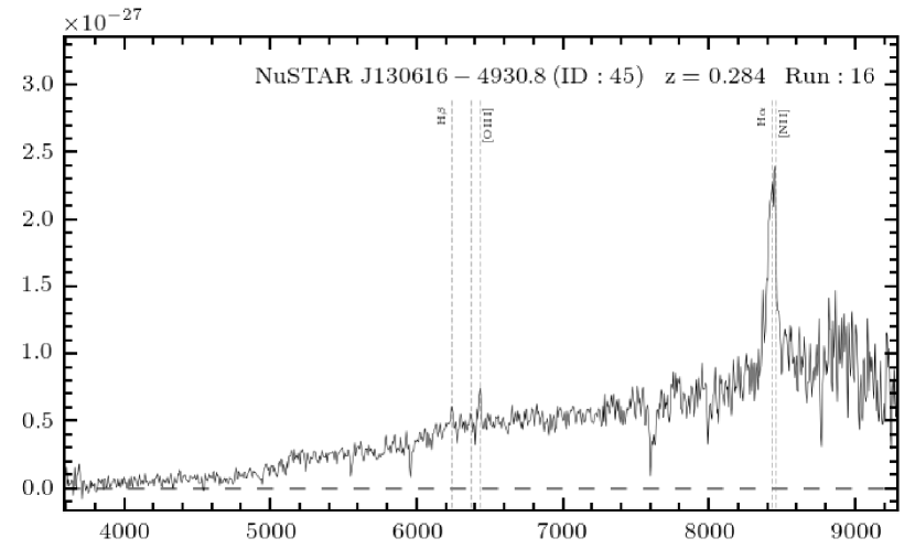
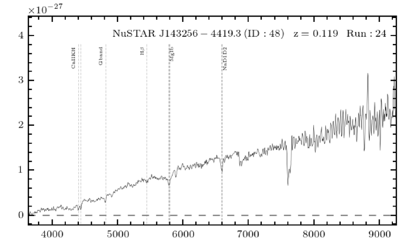
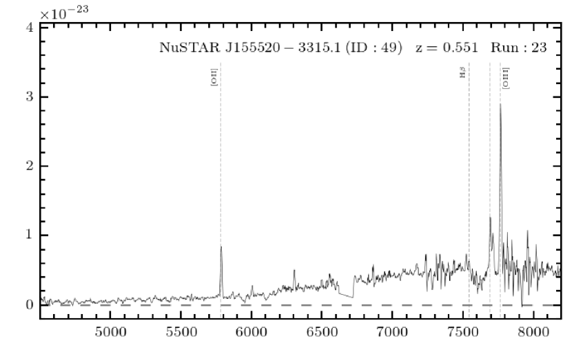
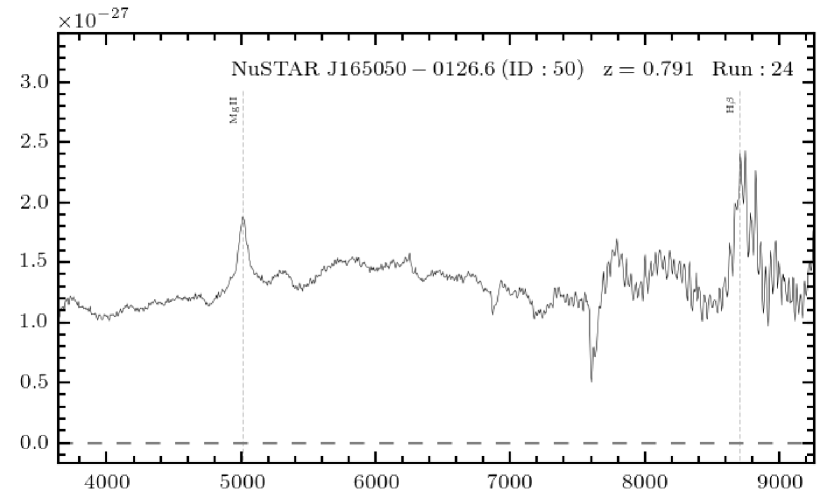
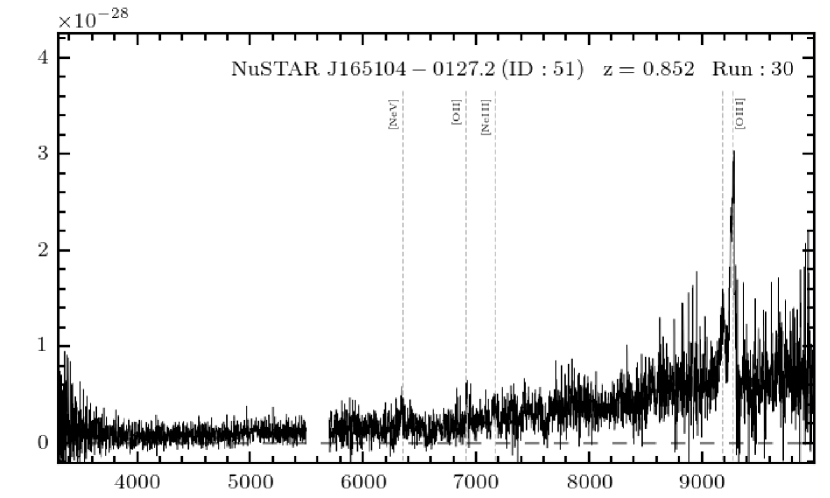
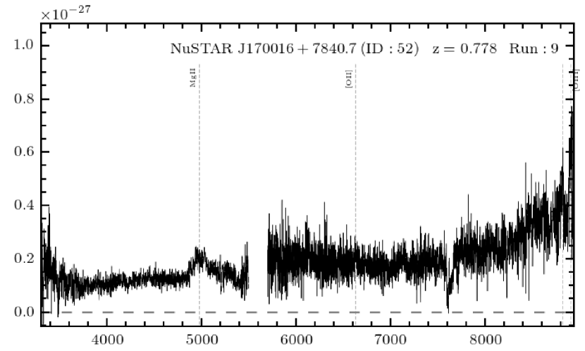
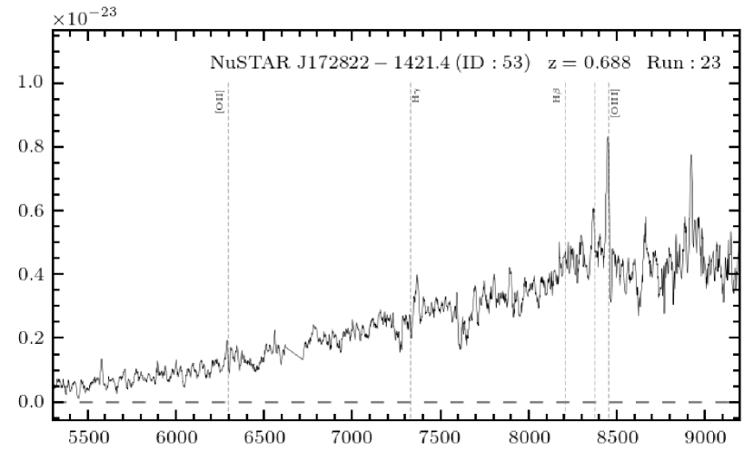
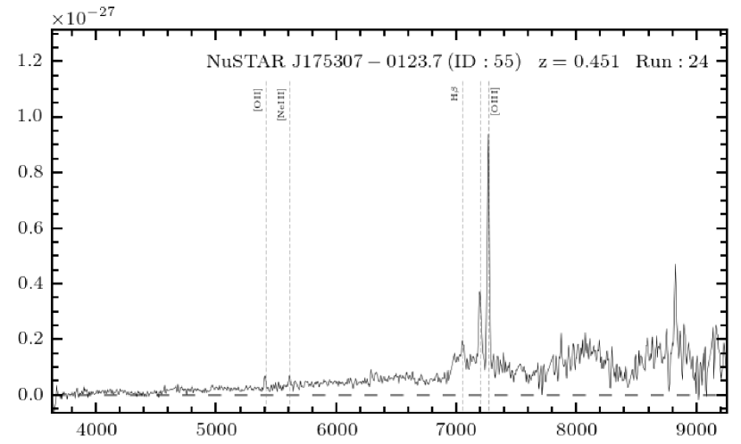
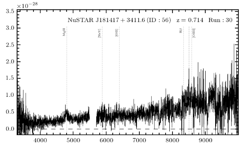
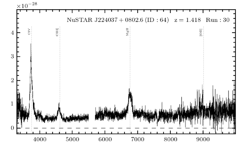
Figure 23.— Continued.

References

- Agüeros et al. (2009) Agüeros, M. A., Anderson, S. F., Covey, K. R., et al. 2009, ApJS, 181, 444
- Aird et al. (2015a) Aird, J., Coil, A. L., Georgakakis, A., et al. 2015a, MNRAS, 451, 1892
- Aird et al. (2015b) Aird, J., Alexander, D. M., Ballantyne, D. R., et al. 2015b, ApJ, 815, 66
- Ajello et al. (2008) Ajello, M., Greiner, J., Kanbach, G., et al. 2008, ApJ, 678, 102
- Akiyama et al. (2000) Akiyama, M., Ohta, K., Yamada, T., et al. 2000, ApJ, 532, 700
- Alexander et al. (2001) Alexander, D. M., Brandt, W. N., Hornschemeier, A. E., et al. 2001, AJ, 122, 2156
- Alexander & Hickox (2012) Alexander, D. M., & Hickox, R. C. 2012, New A Rev., 56, 93
- Alexander et al. (2003) Alexander, D. M., Bauer, F. E., Brandt, W. N., et al. 2003, AJ, 126, 539
- Alexander et al. (2013) Alexander, D. M., Stern, D., Del Moro, A., et al. 2013, ApJ, 773, 125
- Asmus et al. (2015) Asmus, D., Gandhi, P., Hönig, S. F., Smette, A., & Duschl, W. J. 2015, MNRAS, 454, 766
- Assef et al. (2010) Assef, R. J., Kochanek, C. S., Brodwin, M., et al. 2010, ApJ, 713, 970
- Assef et al. (2013) Assef, R. J., Stern, D., Kochanek, C. S., et al. 2013, ApJ, 772, 26
- Ballantyne et al. (2006) Ballantyne, D. R., Everett, J. E., & Murray, N. 2006, ApJ, 639, 740
- Baloković et al. (2014) Baloković, M., Comastri, A., Harrison, F. A., et al. 2014, ApJ, 794, 111
- Barcons et al. (2007) Barcons, X., Carrera, F. J., Ceballos, M. T., et al. 2007, A&A, 476, 1191
- Barger et al. (2003) Barger, A. J., Cowie, L. L., Capak, P., et al. 2003, AJ, 126, 632
- Baumgartner et al. (2013) Baumgartner, W. H., Tueller, J., Markwardt, C. B., et al. 2013, ApJS, 207, 19
- Bertin & Arnouts (1996) Bertin, E., & Arnouts, S. 1996, A&AS, 117, 393
- Boller et al. (1996) Boller, T., Brandt, W. N., & Fink, H. 1996, A&A, 305, 53
- Bottacini et al. (2012) Bottacini, E., Ajello, M., & Greiner, J. 2012, ApJS, 201, 34
- Brandt & Alexander (2015) Brandt, W. N., & Alexander, D. M. 2015, A&A Rev., 23, 1
- Brandt & Hasinger (2005) Brandt, W. N., & Hasinger, G. 2005, ARA&A, 43, 827
- Brandt et al. (1997) Brandt, W. N., Mathur, S., & Elvis, M. 1997, MNRAS, 285, L25
- Burlon et al. (2011) Burlon, D., Ajello, M., Greiner, J., et al. 2011, ApJ, 728, 58
- Caccianiga et al. (2004) Caccianiga, A., Severgnini, P., Braito, V., et al. 2004, A&A, 416, 901
- Caccianiga et al. (2008) Caccianiga, A., Severgnini, P., Della Ceca, R., et al. 2008, A&A, 477, 735
- Cardamone et al. (2008) Cardamone, C. N., Urry, C. M., Damen, M., et al. 2008, ApJ, 680, 130
- Civano et al. (2015) Civano, F., Hickox, R. C., Puccetti, S., et al. 2015, ApJ, 808, 185
- Comastri et al. (2001) Comastri, A., Fiore, F., Vignali, C., et al. 2001, MNRAS, 327, 781
- Comastri et al. (2002) Comastri, A., Vignali, C., Brusa, M., Hellas, & Hellas2XMM Consortia. 2002, in Astronomical Society of the Pacific Conference Series, Vol. 284, IAU Colloq. 184: AGN Surveys, ed. R. F. Green, E. Y. Khachikian, & D. B. Sanders, 235
- de Carvalho et al. (1997) de Carvalho, R. R., Ribeiro, A. L. B., Capelato, H. V., & Zepf, S. E. 1997, ApJS, 110, 1
- Del Moro et al. (2008) Del Moro, A., Mateos, S., Watson, M. G., & Akiyama, M. 2008, in 8th National Conference on AGN, ed. L. Lanteri, C. M. Raiteri, A. Capetti, & P. Rossi
- Del Moro et al. (2014) Del Moro, A., Mullaney, J. R., Alexander, D. M., et al. 2014, ApJ, 786, 16
- Della Ceca et al. (1999) Della Ceca, R., Castelli, G., Braito, V., Cagnoni, I., & Maccacaro, T. 1999, ApJ, 524, 674
- Dickinson et al. (2003) Dickinson, M., Giavalisco, M., & GOODS Team. 2003, in The Mass of Galaxies at Low and High Redshift, ed. R. Bender & A. Renzini, 324
- Eckart et al. (2010) Eckart, M. E., McGreer, I. D., Stern, D., Harrison, F. A., & Helfand, D. J. 2010, ApJ, 708, 584
- Eckart et al. (2006) Eckart, M. E., Stern, D., Helfand, D. J., et al. 2006, ApJS, 165, 19
- Evans et al. (2010) Evans, I. N., Primini, F. A., Glotfelty, K. J., et al. 2010, ApJS, 189, 37
- Evans et al. (2014) Evans, P. A., Osborne, J. P., Beardmore, A. P., et al. 2014, ApJS, 210, 8
- Fabian & Barcons (1992) Fabian, A. C., & Barcons, X. 1992, ARA&A, 30, 429
- Fiore et al. (2001) Fiore, F., Giommi, P., Vignali, C., et al. 2001, MNRAS, 327, 771
- Fiore et al. (2003) Fiore, F., Brusa, M., Cocchia, F., et al. 2003, A&A, 409, 79
- Fiore et al. (2009) Fiore, F., Puccetti, S., Brusa, M., et al. 2009, ApJ, 693, 447
- Freeman et al. (2002) Freeman, P. E., Kashyap, V., Rosner, R., & Lamb, D. Q. 2002, ApJS, 138, 185
- Fruscione et al. (2006) Fruscione, A., McDowell, J. C., Allen, G. E., et al. 2006, in Society of Photo-Optical Instrumentation Engineers (SPIE) Conference Series, Vol. 6270, Society of Photo-Optical Instrumentation Engineers (SPIE) Conference Series
- Gandhi et al. (2004) Gandhi, P., Crawford, C. S., Fabian, A. C., & Johnstone, R. M. 2004, MNRAS, 348, 529
- Gandhi et al. (2009) Gandhi, P., Horst, H., Smette, A., et al. 2009, A&A, 502, 457
- Gandhi et al. (2014) Gandhi, P., Lansbury, G. B., Alexander, D. M., et al. 2014, ApJ, 792, 117
- Gehrels (1986) Gehrels, N. 1986, ApJ, 303, 336
- Giacconi et al. (1979) Giacconi, R., Bechtold, J., Branduardi, G., et al. 1979, ApJ, 234, L1
- Gioia et al. (1990) Gioia, I. M., Maccacaro, T., Schild, R. E., et al. 1990, ApJS, 72, 567
- Goodrich (1989) Goodrich, R. W. 1989, ApJ, 342, 224
- Groth et al. (1994) Groth, E. J., Kristian, J. A., Lynds, R., et al. 1994, in Bulletin of the American Astronomical Society, Vol. 26, American Astronomical Society Meeting Abstracts, 1403
- Hao et al. (2010) Hao, H., Elvis, M., Civano, F., et al. 2010, ApJ, 724, L59
- Harrison et al. (2003) Harrison, F. A., Eckart, M. E., Mao, P. H., Helfand, D. J., & Stern, D. 2003, ApJ, 596, 944
- Harrison et al. (2013) Harrison, F. A., Craig, W. W., Christensen, F. E., et al. 2013, ApJ, 770, 103
- Harrison et al. (2016) Harrison, F. A., Aird, J., Civano, F., et al. 2016, ApJ, 831, 185
- Hasinger (2008) Hasinger, G. 2008, A&A, 490, 905
- Hasinger et al. (2005) Hasinger, G., Miyaji, T., & Schmidt, M. 2005, A&A, 441, 417
- Hickox & Markevitch (2006) Hickox, R. C., & Markevitch, M. 2006, ApJ, 645, 95
- Hong et al. (2016) Hong, J., Mori, K., Hailey, C. J., et al. 2016, ApJ, 825, 132
- Hornschemeier et al. (2001) Hornschemeier, A. E., Brandt, W. N., Garmire, G. P., et al. 2001, ApJ, 554, 742
- Huchra et al. (2012) Huchra, J. P., Macri, L. M., Masters, K. L., et al. 2012, ApJS, 199, 26
- Ichikawa et al. (2012) Ichikawa, K., Ueda, Y., Terashima, Y., et al. 2012, ApJ, 754, 45
- Jarrett et al. (2011) Jarrett, T. H., Cohen, M., Masci, F., et al. 2011, ApJ, 735, 112
- Jones et al. (2004) Jones, D. H., Saunders, W., Colless, M., et al. 2004, MNRAS, 355, 747
- Jones et al. (2009) Jones, D. H., Read, M. A., Saunders, W., et al. 2009, MNRAS, 399, 683
- Jun & Im (2013) Jun, H. D., & Im, M. 2013, ApJ, 779, 104
- Kim et al. (2004) Kim, D.-W., Cameron, R. A., Drake, J. J., et al. 2004, ApJS, 150, 19
- Komatsu et al. (2011) Komatsu, E., Smith, K. M., Dunkley, J., et al. 2011, ApJS, 192, 18
- Koss et al. (2013) Koss, M., Mushotzky, R., Baumgartner, W., et al. 2013, ApJ, 765, L26
- Koss et al. (2016) Koss, M. J., Glidden, A., Baloković, M., et al. 2016, ApJ, 824, L4
- Kraft et al. (1991) Kraft, R. P., Burrows, D. N., & Nousek, J. A. 1991, ApJ, 374, 344
- Krivonos et al. (2007) Krivonos, R., Revnivtsev, M., Lutovinov, A., et al. 2007, A&A, 475, 775
- Krivonos et al. (2015) Krivonos, R. A., Tsygankov, S. S., Lutovinov, A. A., et al. 2015, ApJ, 809, 140
- La Franca et al. (2005) La Franca, F., Fiore, F., Comastri, A., et al. 2005, ApJ, 635, 864
- Laird et al. (2009) Laird, E. S., Nandra, K., Georgakakis, A., et al. 2009, ApJS, 180, 102
- LaMassa et al. (2016) LaMassa, S. M., Ricarte, A., Glikman, E., et al. 2016, ApJ, 820, 70
- Lansbury et al. (2014) Lansbury, G. B., Alexander, D. M., Del Moro, A., et al. 2014, ApJ, 785, 17
- Lansbury et al. (2015) Lansbury, G. B., Gandhi, P., Alexander, D. M., et al. 2015, ApJ, 809, 115
- Lanzuisi et al. (2009) Lanzuisi, G., Piconcelli, E., Fiore, F., et al. 2009, A&A, 498, 67
- Lanzuisi et al. (2015) Lanzuisi, G., Ranalli, P., Georgantopoulos, I., et al. 2015, A&A, 573, A137
- Lawrence et al. (2007) Lawrence, A., Warren, S. J., Almaini, O., et al. 2007, MNRAS, 379, 1599
- Lehmann et al. (2001) Lehmann, I., Hasinger, G., Schmidt, M., et al. 2001, A&A, 371, 833
- Lehmer et al. (2005) Lehmer, B. D., Brandt, W. N., Alexander, D. M., et al. 2005, ApJS, 161, 21
- Leighly et al. (2007a) Leighly, K. M., Halpern, J. P., Jenkins, E. B., & Casebeer, D. 2007a, ApJS, 173, 1
- Leighly et al. (2007b) Leighly, K. M., Halpern, J. P., Jenkins, E. B., et al. 2007b, ApJ, 663, 103
- Luo et al. (2014) Luo, B., Brandt, W. N., Alexander, D. M., et al. 2014, ApJ, 794, 70
- Lutz et al. (2004) Lutz, D., Maiolino, R., Spoon, H. W. W., & Moorwood, A. F. M. 2004, A&A, 418, 465
- Maccacaro et al. (1988) Maccacaro, T., Gioia, I. M., Wolter, A., Zamorani, G., & Stocke, J. T. 1988, ApJ, 326, 680
- Malizia et al. (2012) Malizia, A., Bassani, L., Bazzano, A., et al. 2012, MNRAS, 426, 1750
- Markowitz et al. (2014) Markowitz, A. G., Krumpe, M., & Nikutta, R. 2014, MNRAS, 439, 1403
- Massaro et al. (2009) Massaro, E., Giommi, P., Leto, C., et al. 2009, A&A, 495, 691
- Mateos et al. (2013) Mateos, S., Alonso-Herrero, A., Carrera, F. J., et al. 2013, MNRAS, 434, 941
- Mateos et al. (2008) Mateos, S., Warwick, R. S., Carrera, F. J., et al. 2008, A&A, 492, 51
- Mateos et al. (2012) Mateos, S., Alonso-Herrero, A., Carrera, F. J., et al. 2012, MNRAS, 426, 3271
- Mateos et al. (2015) Mateos, S., Carrera, F. J., Alonso-Herrero, A., et al. 2015, MNRAS, 449, 1422
- Mathur (2000) Mathur, S. 2000, MNRAS, 314, L17
- Matsuta et al. (2012) Matsuta, K., Gandhi, P., Dotani, T., et al. 2012, ApJ, 753, 104
- McHardy et al. (2003) McHardy, I. M., Gunn, K. F., Newsam, A. M., et al. 2003, MNRAS, 342, 802
- Merloni et al. (2014) Merloni, A., Bongiorno, A., Brusa, M., et al. 2014, MNRAS, 437, 3550
- Miniutti et al. (2012) Miniutti, G., Brandt, W. N., Schneider, D. P., et al. 2012, MNRAS, 425, 1718
- Monet et al. (2003) Monet, D. G., Levine, S. E., Canzian, B., et al. 2003, AJ, 125, 984
- Moretti et al. (2006) Moretti, A., Perri, M., Capalbi, M., et al. 2006, A&A, 448, L9
- Mori et al. (2015) Mori, K., Hailey, C. J., Krivonos, R., et al. 2015, ApJ, 814, 94
- Morris et al. (1991) Morris, S. L., Stocke, J. T., Gioia, I. M., et al. 1991, ApJ, 380, 49
- Mullaney et al. (2015) Mullaney, J. R., Del-Moro, A., Aird, J., et al. 2015, ApJ, 808, 184
- Mushotzky et al. (2000) Mushotzky, R. F., Cowie, L. L., Barger, A. J., & Arnaud, K. A. 2000, Nature, 404, 459
- Nandra et al. (2003) Nandra, K., Georgantopoulos, I., Ptak, A., & Turner, T. J. 2003, ApJ, 582, 615
- Nandra et al. (2005) Nandra, K., Laird, E. S., Adelberger, K., et al. 2005, MNRAS, 356, 568
- Pietsch et al. (1998) Pietsch, W., Bischoff, K., Boller, T., et al. 1998, A&A, 333, 48
- Pounds et al. (1995) Pounds, K. A., Done, C., & Osborne, J. P. 1995, MNRAS, 277, L5
- Radburn-Smith et al. (2006) Radburn-Smith, D. J., Lucey, J. R., Woudt, P. A., Kraan-Korteweg, R. C., & Watson, F. G. 2006, MNRAS, 369, 1131
- Ricci et al. (2015) Ricci, C., Ueda, Y., Koss, M. J., et al. 2015, ApJ, 815, L13
- Risaliti et al. (2005) Risaliti, G., Elvis, M., Fabbiano, G., Baldi, A., & Zezas, A. 2005, ApJ, 623, L93
- Rosen et al. (2016) Rosen, S. R., Webb, N. A., Watson, M. G., et al. 2016, A&A, 590, A1
- Schmidt & Green (1983) Schmidt, M., & Green, R. F. 1983, ApJ, 269, 352
- Schmidt et al. (1998) Schmidt, M., Hasinger, G., Gunn, J., et al. 1998, A&A, 329, 495
- Scoville et al. (2007) Scoville, N., Aussel, H., Brusa, M., et al. 2007, ApJS, 172, 1
- Stern (2015) Stern, D. 2015, ApJ, 807, 129
- Stern et al. (2012) Stern, D., Assef, R. J., Benford, D. J., et al. 2012, ApJ, 753, 30
- Stern et al. (2014) Stern, D., Lansbury, G. B., Assef, R. J., et al. 2014, ApJ, 794, 102
- Stickel et al. (1993) Stickel, M., Kuehr, H., & Fried, J. W. 1993, A&AS, 97, 483
- Tingay et al. (2003) Tingay, S. J., Jauncey, D. L., King, E. A., et al. 2003, PASJ, 55, 351
- Tozzi et al. (2001) Tozzi, P., Rosati, P., Nonino, M., et al. 2001, ApJ, 562, 42
- Treister & Urry (2006) Treister, E., & Urry, C. M. 2006, ApJ, 652, L79
- Treister et al. (2004) Treister, E., Urry, C. M., Chatzichristou, E., et al. 2004, ApJ, 616, 123
- Tueller et al. (2008) Tueller, J., Mushotzky, R. F., Barthelmy, S., et al. 2008, ApJ, 681, 113
- Ueda et al. (2005) Ueda, Y., Ishisaki, Y., Takahashi, T., Makishima, K., & Ohashi, T. 2005, ApJS, 161, 185
- Ueda et al. (1999) Ueda, Y., Takahashi, T., Inoue, H., et al. 1999, ApJ, 518, 656
- Vasudevan et al. (2013) Vasudevan, R. V., Brandt, W. N., Mushotzky, R. F., et al. 2013, ApJ, 763, 111
- Watson et al. (2009) Watson, M. G., Schröder, A. C., Fyfe, D., et al. 2009, A&A, 493, 339
- Wik et al. (2014) Wik, D. R., Hornstrup, A., Molendi, S., et al. 2014, ApJ, 792, 48
- Wong et al. (2008) Wong, D. S., Chornock, R., & Filippenko, A. V. 2008, PASP, 120, 266
- Worsley et al. (2005) Worsley, M. A., Fabian, A. C., Bauer, F. E., et al. 2005, MNRAS, 357, 1281
- Wright et al. (2010) Wright, E. L., Eisenhardt, P. R. M., Mainzer, A. K., et al. 2010, AJ, 140, 1868
- Xue et al. (2011) Xue, Y. Q., Luo, B., Brandt, W. N., et al. 2011, ApJS, 195, 10
- Xue et al. (2012) Xue, Y. Q., Wang, S. X., Brandt, W. N., et al. 2012, ApJ, 758, 129
- York et al. (2000) York, D. G., Adelman, J., Anderson, Jr., J. E., et al. 2000, AJ, 120, 1579
- Younes et al. (2012) Younes, G., Kouveliotou, C., Kargaltsev, O., et al. 2012, ApJ, 757, 39
- Zhou et al. (2006) Zhou, H., Wang, T., Yuan, W., et al. 2006, ApJS, 166, 128