On the influence of a Hybrid Thermal-Non thermal distribution in the Internal Shocks model for blazars

Abstract

Internal shocks occurring in blazars may accelerate both thermal and non-thermal electrons. In this paper we examine the consequences that such a hybrid (thermal/non-thermal) EED has on the spectrum of blazars. Since the thermal component of the EED may extend to very low energies. We replace the standard synchrotron process by the more general magneto-bremsstrahlung (MBS). Significant differences in the energy flux appear at low radio frequencies when considering MBS instead of the standard synchrotron emission. A drop in the spectrum appears in the all the radio band and a prominent valley between the infrared and soft X-rays bands when a hybrid EED is considered, instead of a power-law EED. In the $\gamma$-ray band an EED of mostly thermal particles displays significant differences with respect to the one dominated by non-thermal particles. A thermally-dominated EED produces a synchrotron self-Compton (SSC) peak extending only up to a few MeV, and the valley separating the MBS and the SSC peaks is much deeper than if the EED is dominated by non-thermal particles. The combination of these effects modifies the Compton dominance of a blazar, suggesting that the vertical scatter in the distribution of FSRQs and BL Lac objects in the peak synchrotron frequency - Compton dominance parameter space could be attributed to different proportions of thermal/non-thermal particles in the EED of blazars. Finally, the temperature of the electrons in the shocked plasma is shown to be a degenerated quantity for different magentizations of the ejected material.

1 Introduction

In this work we study the emission mechanisms in blazars, a subclass of radio-loud active galactic nuclei (AGN) in which a relativistic jet is propagating in the direction very close to the line of sight towards us (e.g., Urry & Padovani, 1995). An important observed component of the blazar radiation is produced by the non-thermal emission from the relativistic jet they are assumed to host. Its spectrum shows two broad peaks. The first one is located between radio and X-rays and the second one between X-rays and $\gamma$-rays (e.g., Fossati et al., 1998). Depending on the peak frequencies and the strength of the emission lines blazars can be further subdivided into BL Lac objects and flat spectrum radio-quasars (FSRQS; e.g. Giommi et al., 2012). There is a broad consensus that the low frequency peak is due to the synchrotron emission from the relativistic electrons gyrating in a magnetic field. As for the high frequency peak, currently there are two contending models. In the leptonic model the high-energy emission is produced by the relativistic electrons that inverse-Compton upscatter both the external low-frequency photons (external inverse-Compton; EIC), as well as the synchrotron photons produced in the jet (synchrotron self-Compton; SSC). In the hadronic model there are relativistic protons in the jet that, in the presence of very strong magnetic fields, are able to produce the high energy emission both directly (via proton-synchrotron radiation), as well as via electromagnetic cascades (see e.g., Boettcher, 2010, and references therein for a detailed discussion of both models). In this work we limit our discussion to the leptonic model.

The blazar emitted radiation results from the dissipation of the jet kinetic and Poynting flux. In our work we consider the internal shocks (IS) model, in which the aforementioned dissipation is produced by the collision of cold and dense blobs (’shells’) within the jet (e.g., Rees & Meszaros, 1994; Spada et al., 2001; Mimica et al., 2004). Each shell collision can produce IS that accelerate electrons that are ultimately responsible for the observed emission.

In the previous papers on this topic we investigated the influence of the magnetic field on the IS dynamics (Mimica & Aloy, 2010) and emission (Mimica et al., 2007; Mimica & Aloy, 2012; Rueda-Becerril et al., 2014, hereafter, the latter two papers will be referred as MA12 and RMA14, respectively). In this paper we shift our focus to the influence of the properties of the electron energy distribution (EED) on the observed emission. Giannios & Spitkovsky (2009) proposed a mixed Maxwellian/non-thermal EED (’hybrid distribution’ or HD hereafter) as an explanation of some of the features of the gamma-ray burst prompt and afterglow emission. In this paper we introduce a HD into our numerical code and study how it affects the blazar light curves and spectra.

Since the HD thermal component extends to subrelativistic electron energies, we need to reconsider the emission mechanism (synchrotron) we employed in previous works. The radiation from charged particles traversing a magnetic field is known as magnetobremsstrahlung (MBS). Depending on the speed $\beta c$ of the particles, this radiation is categorized into cyclotron radiation if $(\beta\ll 1)$ and synchrotron radiation $(\beta\sim 1)$. Both regimes have been studied broadly and accurate analytical expressions for each have been developed (e.g., Ginzburg & Syrovatskii, 1965; Rybicki & Lightman, 1979; Pacholczyk, 1970). However, the cyclo-synchrotron radiation, i.e., the transrelativistic regime, has no simple analytic description. Therefore, here we implement a cyclo-synchrotron (MBS) emission model in our code, to be able to accurately deal with the emission at all energies of the EED.

In the next section we briefly summarize the dynamics of shell collisions and the resulting IS. In Secs. 3 and 4 we explain how the HD and MBS are included in our numerical models. The spectral differences between the standard synchrotron and MBS, and between a HD and a power-law EED are presented in Sec. 5. In Sec. 6 we describe the results from the parameter study of our model. In Sec. 7 we present the electrons temperature behavior in different IS scenarios. In Sec. 8 we discuss our results and present our conclusions.

2 Shell dynamics and emission in the internal shock model

We model the shell dynamics and the shock properties in blazar jets as in MA12. Assuming a cylindrical outflow and neglecting the jet lateral expansion (it plays a negligible role in blazar jets, see e.g., Mimica et al., 2004) we can simplify the problem of colliding shells to a one-dimensional interaction of two cylindrical shells with cross-sectional radius $R$ and thickness $\Delta r$. The slower (right) shell Lorentz factor is denoted by $\Gamma_{\rm R}$, while the faster (left) shell moves with $\Gamma_{\rm L}=(1+\Delta g)\Gamma_{\rm R}$. In the previous expression $\Delta g$ stands for the relative Lorentz factor between the interacting shells. We assume that the shells are initially cold, so that the fluid thermal pressure ($P$) to rest-mass energy density ratio $\chi:=P/\rho c^{2}\ll 1$, where $\rho$ is the fluid rest-mass density. The shell magnetization is controlled by a parameter $\sigma:=B^{2}/(4\pi\Gamma^{2}\rho c^{2})$, where $B$ is the strength of the large-scale magnetic field (measured in the laboratory frame), that in our model is assumed to be perpendicular to the shell propagation direction. Note that the decay of poloidal fields (i.e., parallel to the shell propagation direction) with distance to the blazar central engine will be faster than that of toroidal fields (perpendicular to the shell propagation direction). Certainly, the rate at which the magnetic field strength may vary with the distance from the blazar central engine depends on the geometry adopted by the jet. If the jet undergoes a conical expansion, a decaying power-law with the distance to the central engine is theoretically expected for the poloidal magnetic field (see e.g., Blandford & Rees, 1974; Königl, 1981). Pure power-law expressions for the decay of the magnetic field are roughly adequate until distances $\sim 1\,$pc from the origin (see e.g., Krichbaum et al., 2006; Beskin & Nokhrina, 2006; McKinney, 2006; Asada & Nakamura, 2012; Nakamura & Asada, 2013; Mohan et al., 2015). Furthermore, any pre-existing magnetic field component perpendicular to the IS will be amplified by the standard MHD shock compression. Thus, we expect that the shells shall possess a magnetic field whose dominant component be perpendicular to the propagation of shell and, hence, our approximation is justified.

The number density in an unshocked shell is given by (see equation 3 of MA12):

$$n_{i}=\displaystyle{\frac{\cal L}{\pi R^{2}m_{p}c^{3}\left[\Gamma_{i}^{2}(1+\epsilon+\chi+\sigma_{i})-\Gamma_{i}\right]\sqrt{1-\Gamma_{i}^{-2}}}}\ ,$$ (1)

where $m_{p}$ and $c$ are the proton mass and the speed of light, $\epsilon$ is the specific internal energy (see equation 2 of MA12), ${\cal L}$ the kinetic luminosity of the shells and the index $i={\rm L,R}$ indicates which shell we are referring to.

Once the number density, the thermal pressure, the magnetization, and the Lorentz factor of both shells have been determined, we use the exact Riemann solver of Romero et al. (2005), suitably modified to account for arbitrarily large magnetizations by Aloy & Mimica (2008), to compute the evolution of the shell collision. In particular, we calculate the properties of the shocked shell fluid (shock velocity, compression factor, magnetic field) which we then use to obtain the synthetic observational signature (see the following section). Both in MA12 and RMA14 it is assumed that a non-thermal EED is injected behind each IS (see e.g., Sec. 3 of MA12), and the code computes the light curve by taking into account the synchrotron, SSC and (if needed) EIC processes (Sec. 4 of MA12). The main modifications introduced by this work are in the hybrid EED injection spectrum and in the replacement of the pure synchrotron by the MBS emission.

3 Hybrid distribution

Most IS models for blazars assume that the radiation is produced by a power-law energy distribution of non-thermal electrons accelerated behind the shock (Spada et al., 2001; Mimica et al., 2004; Böttcher & Dermer, 2010). More specifically, the number density of non-thermal particles per unit time and unit Lorentz factor (both quantities measured in the rest frame of the fluid) is

$$\frac{dn_{{\rm nth}}}{dt\,d\gamma}=Q_{0}\gamma^{-q}H(\gamma;\gamma_{\rm min}^{\rm nth},\gamma_{\rm max}^{\rm nth}),$$ (2)

where $q$ is the power-law index, $\gamma_{\rm min}^{\rm nth}$ and $\gamma_{\rm max}^{\rm nth}$ are lower and upper cut-offs for the Lorentz factor of the injected electrons, respectively, and $Q_{0}$ the normalization coefficient. The interval function is defined as

$$H(x;a,b):=\left\{\begin{array}[]{ll}1,&a\leq x\leq b\\ 0,&\text{elsewhere}\end{array}\right..$$ (3)

As in previous works (Mimica et al. 2010; MA12), $\gamma_{\rm max}^{\rm nth}$ is obtained by assuming that the synchrotron cooling time-scale is proportional to the gyration time-scale,

$$\gamma_{\rm max}^{\rm nth}={\left(\frac{3m_{\rm e}^{2}c^{4}}{4\pi a_{\rm acc}e^{3}B_{\rm S}}\right)}^{1/2},$$ (4)

where $e$ is the electron charge, $m_{\rm e}$ is the electron mass, $B_{\rm S}$ is the total magnetic field in the shock and $a_{\rm acc}\geq 1$ is the acceleration efficiency parameter (Böttcher & Dermer, 2010; Joshi & Böttcher, 2011).

As in MA12 and RMA14, we assume that there exists a stochastic magnetic field, $B_{\rm{S,st}}$, which is created by the shocks produced due to the collision of the shells. By definition its strength is a fraction $\epsilon_{\rm B}$ of the internal energy density of the shocked shell $u_{\rm S}$ (obtained, in our case, by the exact Riemann solver):

$$B_{\rm S,st}=\sqrt{8\pi\epsilon_{\rm B}u_{\rm S}}.$$ (5)

Since we allow for arbitrarily magnetized shells, there is also a macroscopic magnetic field component, $B_{\rm S,mac}$, which is a direct output of the exact Riemann solver. The total magnetic field is then $B:=\sqrt{B^{2}_{\rm S,st}+B^{2}_{\rm S,mac}}$.

The motivation for a HD comes from recent PIC simulations of weakly magnetized relativistic shocks (e.g., Sironi et al., 2013). These simulations find that the energy distribution of particles follows a thermal distribution plus a high energy power-law tail. To describe the energy distribution of relativistic thermal particles we use the normalized Maxwell-Jüttner distribution function (Chandrasekhar, 1939, p. 394) so that the number density of thermal particles per unit time and unit Lorentz factor (both quantities measured in the rest frame of the fluid) reads

$$\frac{dn_{\rm th}}{dt\,d\gamma}=Q_{\rm th}\frac{\gamma^{2}\beta}{\Theta_{\rm e}K_{2}(1/\Theta_{\rm e})}e^{-\gamma/\Theta_{\rm e}},$$ (6)

where $Q_{\rm th}$ is the thermal normalization factor in units of the number density per unit of proper time, $\gamma$ is the Lorentz factor of the electrons, $\beta:={(1-\gamma^{-2})}^{-1/2}$ their velocity, $\Theta_{\rm e}:=k_{\rm B}T/m_{\rm e}c^{2}$ is the dimensionless electron temperature, $k_{\rm B}$ is the Boltzmann constant and $K_{2}(x)$ is the modified Bessel function of second kind. Though the Maxwell-Jütner distribution is valid for any Lorentz factor $\gamma\in[1,\infty]$, for numerical purposes we limit the previous interval to $[\gamma_{\rm min}^{\rm th},\gamma_{\rm max}^{\rm th}]$. We typically employ $\gamma_{\rm min}^{\rm th}=\gamma(\beta=0.01)\simeq 1.00005$ and $\gamma_{\rm max}^{\rm th}\sim 10^{3}$. Giannios & Spitkovsky (2009) proposed an approximation to a HD (in the GRB context) consisting of a thermal distribution below a threshold Lorentz factor and a power-law tail above it. The value of the threshold and the number of particles in each part is determined by a parameter: the proportion of non-thermal particles. A similar approach has been used before by Zdziarski et al. (1990) and Li et al. (1996), splitting the distribution at the mean Lorentz factor of the Maxwell-Jüttner distribution,

$$\langle{\gamma}\rangle=3\Theta_{\rm e}+\frac{K_{1}(1/\Theta_{\rm e})}{K_{2}(1/\Theta_{\rm e})}.$$ (7)

In the standard IS model a fraction $\epsilon_{\rm e}$ of the energy dissipated at the shock accelerates the electrons into a pure power-law distribution. In our study we avoid both finding a break Lorentz factor and estimating the value of $\epsilon_{\rm e}$. Instead we compute the normalization coefficients of each component by assuming that all thermal energy dissipated at the shock is used to accelerate particles. A fraction $\zeta_{\rm e}$ of the energy goes into a non-thermal distribution (the rest going into the thermal part) i.e.,

$$\zeta_{\rm e}\frac{dE_{{\rm inj}}}{dt}=m_{\rm e}c^{2}V_{\rm acc}Q_{0}P(q-1;\gamma_{\rm min}^{\rm nth},\gamma_{\rm max}^{\rm nth}),$$ (8)

where $V_{\rm acc}=\pi R^{2}\Delta r_{\rm acc}$ is the volume where the acceleration takes place (see Sec. 3.2 of MA 12 for more details), $R$ the cross-sectional radius of the cylindrical shells (which we assume for simplicity that have the same diameter as the relativistic jet in which they move), and $Q_{0}$ is the non-thermal normalization factor in units of number density per unit of time. Equation (8) is obtained by integrating equation (2) multiplied by $\gamma m_{\rm e}c^{2}$ in the interval $[\gamma_{\rm min}^{\rm nth},\gamma_{\rm max}^{\rm nth}]$. The function $P$ is defined as

$$P(s;a,b):=\int_{a}^{b}dx\,x^{-s}.$$ (9)

In a similar way, the fraction of energy injected into the thermal part is

$$(1-\zeta_{\rm e})\frac{dE_{{\rm inj}}}{dt}=m_{\rm e}c^{2}V_{\rm acc}Q_{\rm th}\langle{\gamma}\rangle.$$ (10)

Analogously to the injected energy density, the total number density of injected particles per unit of proper time is

$$\frac{dn_{\rm inj}}{dt}=Q_{\rm th}+Q_{0}P(q;\gamma_{\rm min}^{\rm nth},\gamma_{\rm max}^{\rm nth}).$$ (11)

In analogy to equations (10) and (14) in MA12, the total energy and number of particles injection rates into the acceleration region are

$$\frac{dE_{\rm inj}}{dt}= \pi R^{2}u_{\rm S}\beta_{\rm S,CD}c,$$ (12)

$$\frac{dN_{\rm inj}}{dt}= \pi R^{2}n_{i}\Gamma_{i,{\rm CD}}\,\beta_{\rm S,CD}c,$$ (13)

where $u_{\rm S}$ is the internal energy density of the shocked shell, $n_{i}$ is the number density in the shells given by equation (1), $\beta_{\rm S,CD}$ is the speed of the shock (see equation (5) in MA12) and $\Gamma_{i,{\rm CD}}$ is the bulk Lorentz factor of each of the shells measured in the contact discontinuity (CD) frame (see footnote 1).

Assuming that the partition of the number of injected particles is the same as that of the injected energy we set the following relations for the normalization coefficients in equation (11)

$$Q_{0}P(q;\gamma_{\rm min}^{\rm nth},\gamma_{\rm max}^{\rm nth}) :=\zeta_{\rm e}\frac{dn_{\rm inj}}{dt}$$ (14)

$$Q_{th} :=(1-\zeta_{\rm e})\frac{dn_{\rm inj}}{dt}$$ (15)

From equations (14) and (15) we find that

$$Q_{0}=\frac{\zeta_{\rm e}Q_{th}}{(1-\zeta_{\rm e})P(q;\gamma_{\rm min}^{\rm nth},\gamma_{\rm max}^{\rm nth})}.$$ (16)

Finally, from equations (8), (10) and (16) we get the following expression:

$$P(q-1;\gamma_{\rm min}^{\rm nth},\gamma_{\rm max}^{\rm nth})=\langle{\gamma}\rangle P(q;\gamma_{\rm min}^{\rm nth},\gamma_{\rm max}^{\rm nth}),$$ (17)

from which we compute the lower cut-off of the non-thermal distribution $\gamma_{\rm min}^{\rm nth}$ using an iterative procedure. For numerical reasons, we do not allow $\gamma_{\rm min}^{\rm nth}$ to be smaller than $\gamma_{\rm min}^{\rm th}$.

Finally, we define the global bounds bracketing both the thermal and non-thermal EED by

$$\gamma_{1}=\min{(\gamma_{\rm min}^{\rm nth},\gamma_{\rm min}^{\rm th})}\quad\text{and}\quad\gamma_{M}=\max{(\gamma_{\rm max}^{\rm nth},\gamma_{\rm max}^{\rm th})}.$$ (18)

4 Cyclo-synchrotron emission

Including a thermal distribution of particles implies that low-energy electrons will also contribute to the emissivity. Here we develop a formalism that covers the cyclo-synchrotron or MBS emission of both non-relativistic and relativistic electrons.

For an isotropic distribution of electrons $n(\gamma)$ the emissivity takes the form (Rybicki & Lightman, 1979)

$$j_{\nu}=\frac{1}{4\pi}\int_{1}^{\infty}d\gamma\,n(\gamma)P_{\nu}(\gamma)$$ (19)

where $P_{\nu}(\gamma)$ is the radiated power of an electron having a Lorentz factor $\gamma$ and the factor $1/4\pi$ comes from the angular normalization of the isotropic particle distribution function. These electrons will spiral around the magnetic field lines, moving with a pitch angle $\alpha$. The radiated power $P_{\nu}(\gamma)$, in the comoving frame (see footnote 1) is

$$P_{\nu}(\gamma)=\int_{0}^{2\pi}\int_{-1}^{1}d\phi_{\alpha}\,d\mu_{\alpha}\int_{0}^{2\pi}\int_{-1}^{1}d\phi\,d\mu\,\eta_{\nu}(\gamma,\vartheta,\alpha),$$ (20)

where $\phi_{\alpha}$ is the azimuthal pitch angle, $\vartheta$ is the emission angle (the angle between the emitted photon and the magnetic field), $\phi$ the azimuthal emission angle, $\mu=\cos\vartheta$, $\mu_{\alpha}=\cos\alpha$ and the function $\eta_{\nu}$ is (see e.g., Bekefi, 1966; Oster, 1961; Melrose & McPhedran, 1991),

$$\eta_{\nu}(\gamma,\mu,\mu_{\alpha}) = \frac{2\pi e^{2}\nu^{2}}{c}\sum_{m=1}^{\infty}\delta(y_{m})\left[\frac{{(\mu-\beta\mu_{\alpha})}^{2}}{1-\mu^{2}}J^{2}_{m}(z)\right.+$$ (21)

$$+ \left.\beta^{2}(1-\mu_{\alpha}^{2})J^{\prime 2}_{m}(z)\right],$$

where $m$ is an integer index annotating the number of the contributing harmonic,

$$y_{m}:=\frac{m\nu_{b}}{\gamma}-\nu(1-\beta\mu_{\alpha}\mu),$$ (22)

$$z:=\frac{\nu\gamma\beta\sqrt{1-\mu^{2}}\sqrt{1-\mu_{\alpha}^{2}}}{\nu_{b}},$$ (23)

$\nu_{b}:=eB/2\pi m_{\rm e}c$ is the non-relativistic gyrofrequency, $J_{m}(x)$ is the Bessel function of the first kind of order $m$, and $\gamma=1/\sqrt{1-\beta^{2}}$. When the argument in the $\delta$-function $y_{m}$ equals zero we met the so-called resonance condition (also known as the Doppler condition, e.g. Leung et al., 2011; Melrose & McPhedran, 1991)

$$\frac{m\nu_{b}}{\gamma}-\nu(1-\beta\mu_{\alpha}\mu)=0.$$ (24)

The fulfilment of this condition represents the largest contribution to the power emitted. For slow electrons $(\beta\ll 1)$, the terms with small values of $m$ will dominate (manifesting as emission lines), while for ultrarelativistic ones $(\beta\sim 1)$ the peak of the power radiated shifts to larger values and the spectrum turns into a continuum. In Fig. 1 we can observe these features along with the transrelativistic regime. Since $\eta_{\nu}(\gamma,\vartheta,\alpha)$ depends neither on $\phi_{\alpha}$ nor on $\phi$, the corresponding integration is straightforward. The final expression for $P_{\nu}(\gamma)$ is then,

$$P_{\nu}(\gamma) = \frac{8\pi^{3}e^{2}\nu^{2}}{c}\int_{-1}^{1}\int_{-1}^{1}d\mu_{\alpha}d\mu\sum_{m=1}^{\infty}\delta(y_{m})\times$$ (25)

$$\times \left[\frac{{\left(\mu-\beta\mu_{\alpha}\right)}^{2}}{1-\mu^{2}}J^{2}_{m}(z)+\beta^{2}(1-\mu_{\alpha}^{2})J^{\prime 2}_{m}(z)\right].$$

4.1 The numerical treatment

The numerical evaluation of the MBS emission (Eq. (25)) is very challenging because an integral over an infinite sum of functions $J_{m}$ and their derivatives $J_{m}^{\prime}$ needs to be performed. Several techniques have been used to compute such integral. An approximate analytic formula was found by Petrosian (1981) using the steepest-descent method to achieve good accuracy in the cyclotron and synchrotron regimes, but the relative errors in the intermediate regime were between $20$% and $30$%. In the subsequent works an effort has been made to accurately compute the MBS emissivity over the whole frequency range (for a short review see, e.g. Leung et al., 2011).

The method we follow consists in first integrating Eq. (25) trivially over $\mu_{\alpha}$, exploiting the presence of the $\delta$-function. This is the same first step as employed in Leung et al. (2011), but for the Lorentz factors $\gamma$. Then, from the resonance condition (Eq. 24) we find upper and lower boundaries for the summation over harmonics. To be more precise, if $\mu\neq 0$, we solve the resonance condition for $\mu_{\alpha}$,

$$\mu_{\alpha}=\frac{\gamma\nu-m\nu_{b}}{\gamma\nu\beta\mu}=\frac{\gamma{\cal X}-m}{\gamma{\cal X}\beta\mu},$$ (26)

where ${\cal X}:=\nu/\nu_{b}$ is the frequency of the emitted photon in units of the gyrofrequency (also known as the harmonic number). The case $\mu=0$ can be explicitly avoided by performing a numerical integration of Eq. (20) in which none of the quadrature points falls on zero (see below). Since $|\mu_{\alpha}|<1$, the upper and lower boundaries for the summation in Eq. (21) read:

$$m>\gamma{\cal X}(1-\beta\mu),$$ (27)

$$m<\gamma{\cal X}(1+\beta\mu).$$ (28)

Since the values of $m$ must be integer, from equations (27) and (28) we define $m_{+}:=\lfloor\gamma{\cal X}(1+\beta\mu)\rfloor$ and $m_{-}:=\lceil\gamma{\cal X}(1-\beta\mu)\rceil$, obtaining then from Eq. (25),

$$P_{\nu}(\gamma) =\frac{8\pi^{3}e^{2}\nu_{b}{\cal X}^{2}}{c}\int_{-1}^{1}d\mu\,\left(\frac{1}{{\cal X}\beta|\mu|}\right)\times$$

$$\times \sum_{m=m_{-}}^{m_{+}}\left[\frac{{\left(\mu-\beta\mu_{\alpha}\right)}^{2}}{1-\mu^{2}}J^{2}_{m}(z)+\beta^{2}(1-\mu_{\alpha}^{2})J^{\prime 2}_{m}(z)\right].$$ (29)

where the term in parenthesis before the summation symbol is $|dy_{m}/d\mu_{\alpha}|^{-1}$, which comes from the integration of the $\delta$-function. Note that the value of $\mu_{\alpha}$ in Eq. (29) must be replaced by the relation (26).

Let us now define the following functions:

$$I_{1}({\cal X},\gamma) :=\int_{-1}^{1}d\mu\frac{1}{{\cal X}\beta|\mu|}\times$$

$$\times \sum_{m=m_{-}}^{m_{+}}\left[\frac{{\left(\mu-\beta\mu_{\alpha}\right)}^{2}}{1-\mu^{2}}J^{2}_{m}(z)+\beta^{2}(1-\mu_{\alpha}^{2})J^{\prime 2}_{m}(z)\right],$$ (30)

and

$$\tilde{I}_{2}({\cal X},\gamma_{a},\gamma_{b}):=\int_{\gamma_{a}}^{\gamma_{b}}d\gamma\,n(\gamma){\cal X}^{2}I_{1}({\cal X},\gamma).$$ (31)

where $\gamma_{a}$ and $\gamma_{b}$ are generic input values corresponding to the upper and lower values of Lorentz factor interval in which the calculation of equations (30) and (31) will be performed.

In order to compute the emissivity (Eq. (19)) we calculate first ${\cal X}^{2}I_{1}({\cal X},\gamma)$ and store it in a two-dimensional array. To minimize the numerical problems caused by a sharp drop in the power radiated at low Lorentz factors (keeping ${\cal X}$ constant), a cut-offs array $\{\hat{\gamma}_{\min}\}$ is built (see Appendix B). The integration over $\mu$ in Eq. (30) is performed using a Gauss-Legendre quadrature and considering the emission to be isotropic. At this stage the evaluation $\mu=0$ was avoided by taking an even number of nodal points (specifically, 120 nodes). To complete the array, we compute the Chebyshev coefficients in the $\gamma$ direction of ${\cal X}^{2}I_{1}({\cal X},\gamma)$.

The numerical computation of ${\cal X}^{2}I_{1}({\cal X},\gamma)$ can be made more efficient taking advantage of the developments by Schlickeiser & Lerche (2007, hereafter SL07) in order to simplify the computation of the pitch-angle averaged synchrotron power of an electron having Lorentz factor $\gamma$, which can be written in the synchrotron limit $({\cal X}\gg 1)$ as (Crusius & Schlickeiser, 1986):

$$P_{\nu}^{\rm SL07}(\gamma)=1.315\times 10^{-28}\nu_{b}\,x\,CS[x]\>\>\text{erg\, sec}^{-1}\text{cm}^{-3},$$ (32)

where $x:=2{\cal X}/(3\gamma^{2})$. Comparing the previous expression to Eq. (29) and taking into account Eq. (19) one obtains for sufficiently relativistic electrons

$$x\,CS[x]\approx{\cal X}^{2}I_{1}({\cal X},\gamma).$$ (33)

The function $CS[x]$ is approximated by (SL07)

$$CS[x]\simeq\frac{x^{-2/3}}{0.869+x^{1/3}e^{x}},$$ (34)

which can be computed much faster than the function $I_{1}({\cal X},\gamma)$. We can use this fact to replace the evaluation of the latter function by the simpler computation of $CS[x]$ where the appropriate conditions are satisfied. To determine the region of the parameter space $({\cal X},\gamma)$ where Eq. (34) holds with sufficient accuracy we must consider two restrictions. On the one hand, for the first harmonic, which sets the lower limit where the emissivity is non-zero, we find that ${\cal X}_{1}(\gamma)=1/\gamma$. On the other hand, the synchrotron limit (ultrarelativistic limit) happens for $\gamma\gg 1$. For numerical convenience we take $\gamma_{\rm up}=20$ as a threshold to use Eq. (34). For $\gamma>\gamma_{\rm up}$ the evaluation of $I_{1}$ slows down dramatically since the number of harmonic terms needed to accurately compute it (Eq. (30)) rapidly increases. To show the accuracy of the approximations employed in the calculation of $I_{1}$ we consider the following function (see App. A):

$$RMA[x]:=\begin{cases}x\,CS[x]&x>0.53/\gamma^{3}\\ 0&\text{otherwise}\end{cases},$$ (35)

so that, the resulting electron power becomes

$$P_{\nu}^{\rm RMA}(\gamma)=1.315\times 10^{-28}\nu_{b}\,RMA[x]\>\>\text{erg\, sec}^{-1}\text{cm}^{-3},$$ (36)

In Fig. 1 we show the power radiated by single electrons with different velocities or, equivalently, Lorentz factors. In the non-relativistic limit (e.g., for $\beta=0.2$; Fig. 1 violet solid line) the spectrum is dominated by the first few harmonics (first terms in the sum of Eq. (25)), which results in a number of discrete peaks flanked by regions of almost no radiated power. The first harmonic ($m=1$) peaks at ${\cal X}\simeq 1$ (a consequence of the resonance condition, as mentioned above). As the electron velocity increases ($\beta=0.6,0.9$ and $\gamma=5$; Fig. 1 orange, green and blue solid lines, respectively) the gaps between the peaks of the emitted power are progressively filled. In addition, the spectrum broadens towards ever smaller and larger values of ${\cal X}$, and an increasing number of harmonics shows up. At higher Lorentz factors it makes sense to compare the continuum synchrotron approximation for the electron emitting power with the MBS calculation. For that we display the cases with $\gamma=10,\,40$ and 100 in Fig. 1 with lines colored in red, black and brown, respectively. The different line styles of the latter cases correspond to distinct approximations for the computation of the MBS power. Solid lines correspond to the numerical evaluation of Eq. (25) (the most accurate result). Dashed lines depict the computation of the synchrotron power as in SL07 (Eq. (32)). Dotted lines correspond to the emitted power calculated according to Eq. (36). The difference between the three approximations to compute the radiated power decreases as the Lorentz factor increases. Effectively, for $\gamma>\gamma_{\rm up}$, both the exact calculation and the approximation given by $P_{\nu}^{\rm RMA}(\gamma)$ match rather well. Indeed, the difference becomes fairly small for ${\cal X}\gg 1$. The computation of the function $I_{1}$ becomes extremely expensive for large values of ${\cal X}$, because the number of harmonics needed to be taken into account for the emitted power to be computed accurately enough increases dramatically. Thus, in the following we restrict the more precise numerical evaluation of $P_{\nu}(\gamma)$ employing $I_{1}$ (Eq. (30)) to cases in which ${\cal X}\leq 100$ and $\gamma\leq\gamma_{\rm up}$. For ${\cal X}>100$ and $\gamma>\gamma_{\rm up}$ we resort to the $RMA$ function (Eq. (35)) to fill in the tabulated values of $I_{1}$ (see App. B). We note that Eq. (33) can be generalized to $RMA[x]\approx{\cal X}^{2}I_{1}({\cal X},\gamma)$, from which it is obvious that

$$I_{1}({\cal X},\gamma)\approx RMA[x]/{\cal X}^{2}\qquad\text{if}\quad{\cal X}>100.$$ (37)

We also point to the large quantitative and qualitative effect of the cut-off in the emitted power resulting from the use of the $RMA[x]$ function (Eq. (35)) in the evaluation of $P_{\nu}^{\rm RMA}(\gamma)$ (Eq. (36)). This cut-off is in contrast to the non-zero emitted power at low frequencies, a characteristic of the synchrotron (continuum) approximation.

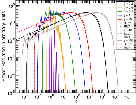
Figure 1: Single electron radiated power as a function of normalized frequency computed for different energies (coloured lines) and with varying degrees of accuracy.

4.2 Numerical evaluation of the emissivity

In this section we describe how an interpolation table is built and afterwards used to compute the emissivity (Eq. (19)) numerically. We discretize the HD by tessellating it in a large number of Lorentz-factor intervals whose boundaries we annotate with ${\{\gamma_{i}\}}_{i=1}^{M}$. Note that the smallest and largest value of the Lorentz factor tessellation coincide with the definitions given in Eq. (18). For numerical convenience and efficiency, in every interval we approximate the EED by a power-law function (with a power-law index $q_{i}$) since, for this particular form it is possible to analytically perform a part of the calculation, which drastically reduces the computational time. Then we use the new interpolation table to compute the emissivity at arbitrary frequency as described below.

4.2.1 The construction of the interpolation table

Performing a direct numerical integration of Eq. (31) may lead to numerical noise in the final result due to the extremely large amplitude oscillations of the integrand in the limits ${\cal X}\ll 1$ and $\gamma\simeq 1$. Therefore, assuming a power-law distribution, we reformulated $\tilde{I}_{2}$ in the following manner

$$I_{2}({\cal X},q,\gamma_{i},\gamma_{i+1}; \gamma_{\rm max}^{\rm th})={\left(\gamma_{\rm max}^{\rm th}\right)}^{1-q}\times$$

$$\times\int_{\gamma_{i}/\gamma_{\rm max}^{\rm th}}^{\gamma_{i+1}/\gamma_{\rm max}^{\rm th}}\mathrm{d}\xi\,\xi^{-q}{\cal X}^{2}I_{1}({\cal X},\xi\gamma_{\rm max}^{\rm th})$$ (38)

where $q$ is the index of the power-law approximation to the EED within the interval $[\gamma_{i},\gamma_{i+1}]$ and $\xi:=\gamma/\gamma_{\rm max}^{\rm th}$. When calculating $\tilde{I}_{2}$ (Eq. (31)), an integral with this shape suggests the definition of

$$I_{3}(\xi,{\cal X},q):=\int_{\xi}^{1}\mathrm{d}\hat{\xi}\,\hat{\xi}^{-q}{\cal X}^{2}I_{1}({\cal X},\hat{\xi}\gamma_{\rm max}^{\rm th}),$$ (39)

where $\hat{\xi}$ is an ancillary variable. Rewriting $I_{2}$ in terms of $I_{3}$ we get

$$\displaystyle I_{2}({\cal X},q,\gamma_{i},\gamma_{i+1}; \,\gamma_{\rm max}^{\rm th})={\left(\gamma_{\rm max}^{\rm th}\right)}^{1-q}\,\times$$

$$\times\left[I_{3}\left(\frac{\gamma_{i}}{\gamma_{\rm max}^{\rm th}},{\cal X},q\right)-I_{3}\left(\frac{\gamma_{i+1}}{\gamma_{\rm max}^{\rm th}},{\cal X},q\right)\right].$$ (40)

We calculate the integral that depends on the three parameters in Eq. (39) resorting to a standard Romberg quadrature method for each value of the triplet $(\xi,{\cal X},q)$. In the same manner as with Eq. (30), a three dimensional array is built for $I_{3}(\xi,{\cal X},q)$ with the Chebyshev coefficients in the $\xi$ direction in order to construct an interpolation table for $I_{2}$ (hereafter disTable).

The integral over Lorentz factors was performed for all values of ${\cal X}$ and $q$ using a Romberg integration routine. Analogously to $\tilde{I}_{1}$ (see App. B.4), the Chebyshev polynomials were constructed in the $\xi$ direction.

4.2.2 Computation of emissivity using an interpolation table

In terms of $I_{2}$ (Eq. 40), the evaluation of the emissivity (Eq. (19)) in any of the power-law segments in which the original distribution has been discretized, e.g., extending between $\gamma_{i}$ and $\gamma_{i+1}$ and having a power-law index $q_{i}$, reads

$$j_{\nu,i}=\frac{\pi e^{2}\nu_{b}}{2c}n(\gamma_{i})\gamma_{i}^{q_{i}}I_{2}\left({\cal X},q_{i},\gamma_{i},\gamma_{i+1};\gamma_{\rm max}^{\rm th}\right).$$ (41)

Then, the total emissivity from an arbitrary EED can efficiently be computed by adding up the contributions from all power-law segments (see e.g. Sec. 4 in Mimica et al., 2009).

The discretization of disTable in the $({\cal X},\xi)$-plane is not uniform. Many more points are explicitly computed in the regime corresponding to low electron energies and emission frequencies than in the rest of the table. In this regime harmonics dominate the emissivity and accurate calculations demand a higher density of tabular points. In the ultrarelativistic regime the emission is computed also numerically. For that we resort to the table produced in MA12 (hereafter uinterp) that includes only the synchrotron process computed with relative errors smaller than $10^{-5}$. Note that in the ultrarelativistic regime the errors made by not including the contribution of the MBS harmonics are negligible. We use both tables in order to cover a wider range of frequencies and Lorentz factors than would be possible if only disTable were to be used (due to the prohibitively expensive calculation for high frequencies and Lorentz factors). In Fig. 2 we sketch the different regions of the ${\cal X}-\xi$ space spanned by our method to assemble a single (large) table. Whenever our calculations require the combination of ${\cal X}$ and $\xi$ that falls in the blue region, we employ disTable to evaluate the emissivity, otherwise we use uinterp. In the particular case when $\gamma_{i}<\gamma_{\rm max}^{\rm th}<\gamma_{i+1}$, the emissivity is computed using both tables as follows:

$$j_{\nu,i}=\frac{\pi e^{2}\nu_{b}}{2c}n(\gamma_{i})\gamma_{i}^{q_{i}}\times \left(I_{2}^{\mathtt{disTable}}({\cal X},q_{i},\gamma_{i},\gamma_{\rm max}^{\rm th};\gamma_{\rm max}^{\rm th})+\right.$$

$$\left.I_{2}^{\mathtt{uinterp}}({\cal X},q_{i},\gamma_{\rm max}^{\rm th},\gamma_{i+1};\gamma_{\rm max}^{\rm th})\right).$$ (42)

Figure 2: Illustration of the different regions of the ${\cal X}-\xi$ space spanned by the distinct approximations employed to compute the values of emissivity according to Eq. (41). ${\cal X}_{\min}$ and ${\cal X}_{\max}$ are generic values for upper and lower limits of ${\cal X}$ for the table disTable and $\xi_{\min}\equiv\gamma_{\rm min}^{\rm th}/\gamma_{\rm max}^{\rm th}$. For a given $q$, a combination of $\xi$ and ${\cal X}$ in the blue region means that disTable is employed. The red area corresponds to the physically forbidden regime where $\gamma<1$ and, therefore, there is no MBS emission. The thin orange strap corresponds to the area of low speeds $1\leq\gamma<\gamma_{1}$ excluded from the table.

5 Differences between MBS and standard synchrotron spectra

In this section we show the importance of the introduction of the new MBS method into our blazar model. We will first show the differences that arise from using different approximations for the emission process assuming the same HD with a dominant non-thermal component (Sect. 5.1) for each test. In the second test we compare the spectra produced by a non-thermally dominated HD with that of a pure power-law extending towards $\gamma_{1}\simeq 1$ (Sect. 5.2) by computing both MBS and pure synchrotron emission.

For the evolution of the particles injected at shocks, we assume that the dominant processes are the synchrotron cooling and the inverse-Compton scattering off the photons produced by the MBS processes (SSC). We note that, in many cases, SSC cooling may be stronger than synchrotron cooling, as we shall see in Sect. 6. To compute synthetic time-dependent multiwavelength spectra and light curves, we include synchrotron and synchrotron self-Compton emission processes resulting from the shocked plasma. We further consider that the observer’s line of sight makes an angle $\theta$ with the jet axis. A detailed description of how the integration of the radiative transfer equation along the line of sight is performed can be found in Section 4 of MA12.

To avoid repeated writing of the parameter values when referring to our models, we introduce a naming scheme in which the magnetization is denoted by the letters S, M and W, referring to the following families of models:

• weakly magnetized, $\sigma_{\rm L}=10^{-6},\sigma_{\rm R}=10^{-6}$,

• moderately magnetized, $\sigma_{\rm L}=10^{-2},\sigma_{\rm R}=10^{-2}$, and

• strongly magnetized, $\sigma_{\rm L}=10^{-1},\sigma_{\rm R}=10^{-1}$.

The remaining four parameters ${\cal L}$, $\Gamma_{\rm R}$, $\Delta g$ and $\zeta_{\rm e}$ can take any of the values shown in Table 1. When we refer to a particular model we label it by appending values of each of these parameters to the model letter. For the parameter $\zeta_{\rm e}$ we use Zm2, Zm1 and Z09 to refer to the values $\zeta_{\rm e}=10^{-2},10^{-1}$ and $0.9$, respectively. Similarly, for the luminosity we write $\boldsymbol{\mathcal{L}}$1, $\boldsymbol{\mathcal{L}}$5, and $\boldsymbol{\mathcal{L}}$50 to denote the values $10^{47}\,\mathrm{erg}\,\mathrm{s}^{-1}$, $5\times 10^{47}\,\mathrm{erg}\,\mathrm{s}^{-1}$ and $5\times 10^{48}\,\mathrm{erg}\,\mathrm{s}^{-1}$, respectively. In this notation, W-G10-D1.0-Zm1-$\boldsymbol{\mathcal{L}}$5 corresponds to the weakly magnetized model with $\Gamma_{\rm R}=10$ (G10), $\Delta g=1.0$ (D1.0), $\zeta_{\rm e}=0.1$ (Zm1) and ${\cal L}=5\times 10^{47}\,\mathrm{erg}\,\mathrm{s}^{-1}$ ($\boldsymbol{\mathcal{L}}$5).

5.1 Spectral differences varying the emissivity for a fixed HD

In Fig. 3 we display the instantaneous spectra of a weakly magnetized model containing a HD where 90% of the particles populate the non-thermal tail of the EED (model W-G10-D1.0-Z09-$\boldsymbol{\mathcal{L}}$1) taken at $10$, $10^{2}$, $10^{3}$, $10^{4}$ and $10^{5}$ seconds after the start of the shell collision. Solid, dotted and dashed lines show the emission computed using the full MBS method (Sec. 4.1) and the direct numerical integration of the analytic approximations $RMA[x]$ (Eq. 35) and the numerical integration of the Crusius & Schlickeiser (1986) function employed in MA12 and RMA14 (referred hereafter as the standard synchrotron), respectively. The difference between the first two and the third is in the presence of a low-frequency cut-off which causes appreciable differences at early times. The purely synchrotron emission (dot-dashed lines) always produces an excess of emission with respect to the other two. This is explained by the fact that there is always a portion of the EED whose energy is too low for it to be emitting in the observed frequencies in a more realistic MBS model (see Fig. 1). The approximate formula $RMA[x]$ performs quite well and its spectra mostly overlap the MBS ones, except close to the first turnover in the spectrum (corresponding to the maximum of the emission from the lowest-energy electrons). Despite the presence of a cutoff in $RMA[x]$, it still overestimates the low-frequency emission just below the first harmonic, which explains the observed slight mismatch.

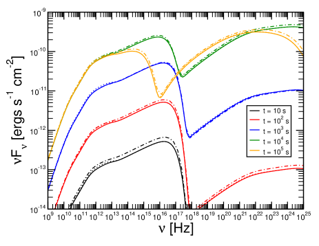
Figure 3: Instantaneous spectra for a model including a HD in which 90% of the particles populate the non-thermal tail of the EED computed employing our new MBS numerical method (full lines), using the direct numerical integration of $RMA[x]$ function (dotted lines, see Eq. 35), and using the direct numerical integration of the Crusius & Schlickeiser (1986) function (dot-dashed lines). The dynamical model employed corresponds to a collision of weakly magnetized shells.

5.2 Spectral differences between an HD and a pure power-law EED

In the previous section we have seen that the differences between the MBS emissivity and the pure synchrotron emissivity are relatively mild if we consider a hybrid, non-thermally dominated EED. To a large extend this happens because a HD is flanked by a monotonically decaying tail at low electron energies (which indeed goes to zero as the electron Lorentz factor approaches 1, see inset of Fig. 4). Here we are interested in outlining the spectral differences when the lower boundary of the EED is varied. For that we consider two different EEDs, namely, a non-thermally dominated HD (corresponding to model W-G10-D1.0-Z09-$\boldsymbol{\mathcal{L}}$1) and a pure power-law EED extending to $\gamma_{1}\simeq 1$. The rest of the parameters of our model, including the MBS emissivity are fixed. To set up the pure power-law EED we cannot follow exactly the same procedure as outlined in Sect. 3 because we must fix $\gamma_{1}$ instead of obtaining it numerically solving Eq. 17. Furthermore, we employ the same non-thermal normalization factor $Q_{0}$ for both the pure power-law EED and the HD.

In Fig. 4 we show the spectral energy distribution corresponding to both the HD and pure power-law EED cases. It is evident that there are substantial differences at frequencies below the GHz range and in the infrared-to-X-rays band. On the other hand, the synchrotron tails above $\sim 10^{13}$ Hz are almost identical for both EED. Correspondingly, the cyclo-synchrotron photons there produced are inverse Compton upscattered forming nearly identical SSC tails above $\sim 10^{20}$ Hz.

5.3 Spectral differences between MBS and pure synchrotron for the same power-law distribution

In the previous section we pointed out how different the SEDs may result for different distributions. Let us now fix the same injected power-law EED starting from $\gamma_{1}\approx 1$ and evaluate the emissivities corresponding to MBS and pure synchrotron processes. In both cases the SSC is also computed. In Fig. 4 we included the averaged SED from a simulation with the same configuration as the pure power-law EED model mentioned above but the radiation treatment was numerical standard synchrotron (green lines). From $10^{10}$ Hz to $10^{22}\,\mathrm{Hz}$ the MBS spectrum is quite similar to that of a pure synchrotron one, so that both emission models are observationally indistinguishable in the latter broad frequecy range. On the other hand, if we look into the MHz band, we will find what we call the cyclotron break, which is the diminishing of the emissivity from each electron due to the cut-off that happens at frequencies below $\nu_{b}$.

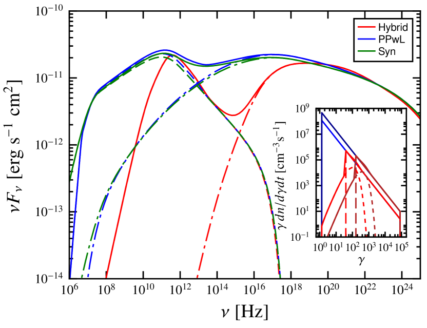
Figure 4: Comparison between the same hybrid model as in Fig. 3 and a pure power-law distribution with $\gamma_{\rm min}^{\rm nth}\simeq 1$. The red lines correspond to the former model while the green and blue lines correspond to simulations with the latter distributions using our MBS numerical method and numerical integration of Crusius & Schlickeiser (1986), respectively. Dashed and dot dashed lines show the synchtron and SSC spectral contributions to each of the respective models. Inset: the injected EEDs in each shock. Blue and dark blue colors correspond to the EED for a pure power-law distribution injected at the FS and at the RS, respectively. Red and dark red colors correspond to the HD distribution injected at the FS and at the RS, respectively.

6 Parameter study

In order to assess the impact of the presence of a hybrid distribution composed by thermal and non-thermal electrons we have performed a parametric study varying a number of intrinsic properties of the shells. In the following subsections we examine the most important results of our parametric study. In the Tab. 1 we show the values of the parameters used in the present work. Some of them are fixed in the following and are shown with a single value in Tab. 1. Among such parameters, we find the fraction of the internal energy density of the shocked shell converted into stochastic magnetic field energy density, $\epsilon_{\rm B}$, the size of the acceleration zone, $\Delta_{\rm acc}$, and the number of turns around magnetic field lines in the acceleration zone that electrons undergo before they cool down, $a_{\rm acc}$ (see Mimica & Aloy, 2012, for further details). The cross-sectional radius and longitudinal size of the shells are given by the parameters $R$ and $\Delta r$, respectively.

One of the parameters kept constant in the previous studies is the total jet luminosity ${\cal L}$, which we now vary. We performed a number of test calculations to compute the lower and upper limits of ${\cal L}$ that produce a spectrum qualitatively similar to that of the source Mrk 421 (Krawczynski & Treister, 2013). In the Table 1 we show the range of variations of this and other parameters.

We perform our parametric scan for the typical redshift value of Mrk 421, namely, $z=0.031$. The viewing angle is fixed to $5^{\circ}$ in all our models. The SEDs in this work were computed by averaging over a time interval of $10^{7}\,\mathrm{s}$.

Parameter	value
$\Gamma_{\rm R}$	$2,\ 10,\ 20$
$\Delta g$	$1.0,\ 2.0,\ 3.0,\ 5.0$
$\sigma_{\rm L}$	$10^{-6},\ 10^{-2},\ 10^{-1}$
$\sigma_{\rm R}$	$10^{-6},\ 10^{-2},\ 10^{-1}$
$\epsilon_{\rm B}$	$10^{-3}$
$\zeta_{\rm e}$	$10^{-2},\ 10^{-1},\ 0.9$
$q$	$2.6$
$\Delta_{\rm acc}$	$10$
$a_{\rm acc}$	$10^{6}$
${\cal L}$	$10^{47},\ 5\times 10^{47},\$ $5\times 10^{48}\,\mathrm{erg}\,\mathrm{s}^{-1}$
$R$	$3\times 10^{16}$ cm
$\Delta r$	$6\times 10^{13}$ cm
$z$	$0.031$
$\theta$	$5^{\circ}$

Table 1: Model parameters. $\Gamma_{\rm R}$ is the Lorentz factor of the slow shell, $\Delta g:=\Gamma_{\rm L}/\Gamma_{\rm R}-1$ ($\Gamma_{\rm L}$ is the Lorentz factor of the fast shell), $\sigma_{\rm L}$ and $\sigma_{\rm R}$ are the fast and slow shell magnetizations, $\epsilon_{\rm B}$ is the fraction of the internal energy density at shocks that it is assumed to be converted into stochastic magnetic field energy density (Eq. (5)), $\zeta_{e}$ and $q$ are the fraction of electrons accelerated into power-law Lorentz factor (or energy) distribution and its corresponding power-law index${}^{\ref{foot:qval}}$, $\Delta_{\rm acc}$ and $a_{\rm acc}$ are the parameters controlling the shock acceleration efficiency (see Section 3.2 of MA12 for details), ${\cal L}$, $R$ and $\Delta r$ are the jet luminosity, jet radius and the initial width of the shells, $z$ is the redshift of the source and $\theta$ is the viewing angle. Note that $\Gamma_{\rm R}$, $\Delta g$, $\sigma_{\rm L}$, $\sigma_{\rm R}$ and $\zeta_{\rm e}$ can take any of the values indicated.

6.1 The presence of the non-thermal population

The influence of the parameter $\zeta_{\rm e}$ on the blazar emission was examined in Böttcher & Dermer (2010), and is an essential model parameter in MA12 and RMA14 as well (though in the latter two papers it was not varied). In this section we explore its influence it by studying three different fractions of non-thermal particles: $\zeta_{\rm e}=0.9,0.1,0.01$. In Fig. 5 we show the averaged SEDs of the models with the aforementioned values of $\zeta_{\rm e}$ for the weakly (left panel) and moderately (right panel) magnetized shells. In both panels we can appreciate that an EED dominated by non-thermal particles produces a broader SSC component. The SSC component of a thermally-dominated EED (W-G10-D1.0-Z09-$\boldsymbol{\mathcal{L}}$5 and M-G10-D1.0-Z09-$\boldsymbol{\mathcal{L}}$5) displays a steeper synchrotron-SSC valley, and the modelled blazar becomes $\gamma$-rays quiet. The synchrotron peak frequency $\nu_{\rm syn}$ is only very weakly dependent on $\zeta_{\rm e}$. According to their synchrotron peak frequency these models resemble low synchrotron peaked blazars (LSP) (Giommi et al., 2012; Giommi et al., 2013).

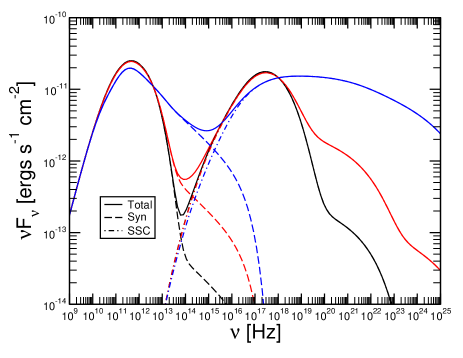
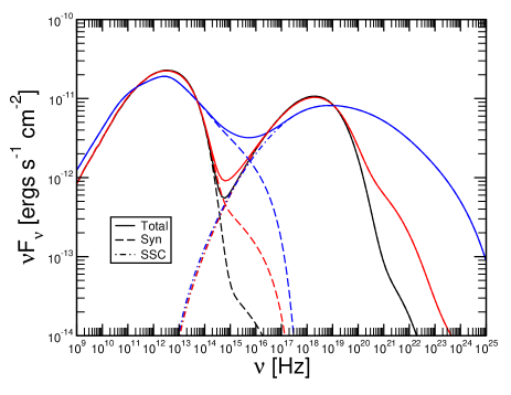
Figure 5: Averaged spectra of the weakly (left panel) and moderately (right panel) magnetized models for $\zeta_{\rm e}=0.9,0.1$ and $0.01$ in blue, red and black lines respectively. Dashed lines show the synchrotron component while the dot-dashed lines show the SSC component.

6.2 Magnetization

In Fig. 6 we show the average spectra produced by the IS model with different combinations of the faster and slower shells magnetizations for a fixed EED with $\zeta_{\rm e}=0.9$. In black, red and blue we represent the models with faster shell magnetization $\sigma_{\rm L}=10^{-6},10^{-2}\mbox{ and }10^{-1}$, respectively. The solid, dotted and dashed lines correspond to a slower shell magnetization $\sigma_{\rm R}=10^{-6},10^{-2}\mbox{ and }10^{-1}$ respectively. Consistent with the results in RMA14, the collision of strongly magnetized shells produces a SSC component dimmer than the synchrotron component. A double bump outline is reproduced by the model M-G10-D1.0-Z09-$\boldsymbol{\mathcal{L}}$1 (dashed, red line) and all the models with $\sigma_{\rm L}=10^{-6}$. For most models $\nu_{\rm syn}$ is situated at $\sim 10^{12}\,$Hz. However, for the cases with $\sigma_{\rm L}=10^{-2},10^{-1}\mbox{ and }\sigma_{\rm R}=10^{-2}$, $\nu_{\rm syn}\sim 10^{13}\,$Hz. In both cases, these frequencies reside in the LSP regime. Remarkably, a change of 4 orders of magnitude in $\sigma_{\rm R}$ results in an increase of $\lesssim 2$ in the observed flux in models with an EED dominated by non-thermal electrons ($\zeta_{\rm e}=0.9$; Fig. 6 left panel). In the case of models with a thermally-dominated EED ($\zeta_{\rm e}=0.1$; Fig. 6 right panel), the change in flux under the same variation of the magnetization of the slower shell is a bit larger, but still by a factor $\lesssim 6$. In both cases the larger differences when changing $\sigma_{\rm R}$ happen in the decaying side of the spectrum occurring to the right of either the synchrotron or the SSC peaks. The variation of the magnetization of the faster shell yields, as expected (MA12; RMA14) larger spectral changes, especially in the SSC part of the spectrum.

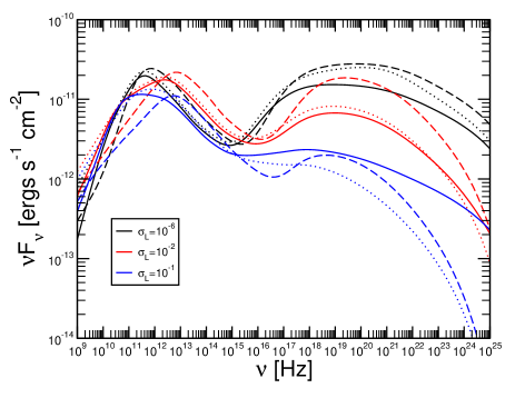
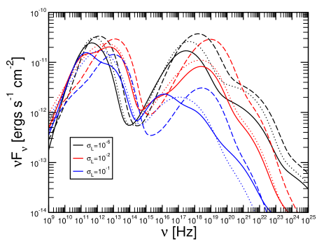
Figure 6: Averaged spectra for different fast shell magnetization, $\sigma_{\rm L}$, with non-thermal particles population fraction $\zeta_{e}=0.9$ and $0.1$ (left and right panels, respectively). The solid, dotted and dashed lines correspond to a magnetization of the slower shell $\sigma_{\rm R}=10^{-6},10^{-2},10^{-1}$, respectively. As was shown in RMA14, the strongly magnetized fast shells do not display a prominent second bump at high frequencies. The synchrotron peak in all cases and in both panels, does not surpass $\sim 10^{13}\,$Hz.

6.3 Relative Lorentz factor $\Delta g$Dg

In Fig. 7 we show the variation of the relative Lorentz factor, $\Delta g$, for $\zeta_{\rm e}=0.1\mbox{ and }0.9$ (W-G10-D(1.0, $\ldots$, 5.0)-Zm1-$\boldsymbol{\mathcal{L}}$1 and W-G10-D(1.0, $\ldots$, 5.0)-Z09-$\boldsymbol{\mathcal{L}}$1). The dashed and dot-dashed lines depict the energy flux coming from the FS and RS, respectively. The model with $\Delta g=1.0$ results from the collision with a fast shell having $\Gamma_{\rm L}=20$, whereas the case $\Delta g=5.0$ assumes that the fast shell moves with $\Gamma_{\rm L}=60$ (i.e., slightly above the upper end of the Lorentz factor distribution for parsec-scale jets; Lister et al. 2016). Both panels show that the larger the $\Delta g$, the higher the SSC bump. The colliding shells with relative Lorentz factor $\Delta g=5.0$ produced a spectrum with an SSC component one order of magnitude larger than its synchrotron component. On the other hand, the colliding shells with relative Lorentz factor $\Delta g=1.0$ produced a SSC component less intense than the synchrotron component. Another important feature in these spectra is the emergence of a second bump in the synchrotron component at the near infrared ($\sim 10^{14}\,\mathrm{Hz}$), which corresponds to emission coming from the reverse shock. The effect of changing $\zeta_{\rm e}$ at high frequencies is that the larger the non-thermal population of electrons the broader the SSC component. Moreover, it can be seen that the forward shock (FS) cannot by itself reproduce the double bump structure of the SED for blazars, and that the emission coming from the reverse shock (RS) dominates and clearly shapes the overall spectrum. More specifically, the emission due to the RS is $\gamma$-ray louder than that of the FS.

The inclusion of a thermal population in the EED combined with a variation of the relative shell Lorentz factor has a potentially measurable impact on the blazar spectra modelling. If narrower SSC peaks and a much steeper decay post-maximum are observed, that could identify the presence of a dominant thermal emission (Fig. 7; right). The slope of the $\gamma$-to-TeV spectrum becomes steeper and more monotonically decaying as $\Delta g$ increases for thermally-dominated EEDs.

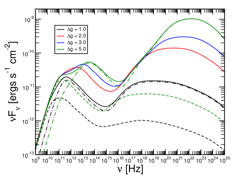
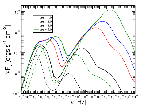
Figure 7: Averaged spectra for different relative Lorentz factors and fractions of non-thermal particles. On the left panel we present the SED from a particle distribution with $\zeta_{\rm e}=0.9$ while on the right panel we show the SED for the same conditions, but with $\zeta_{\rm e}=0.1$. For the models with $\Delta g=1.0$ (black lines) and $\Delta g=5.0$ (green lines) the FS and the RS individual contributions are depicted in dashed and dot-dashed lines, respectively. The models depicted are W-G10-D(1.0, $\ldots$, 5.0)-Z09-$\boldsymbol{\mathcal{L}}$1 (left panel) and W-G10-D(1.0, $\ldots$, 5.0)-Zm1-$\boldsymbol{\mathcal{L}}$1 (right panel).

6.4 Lorentz factor of the slower shell

In Fig. 8 we depict the SEDs resulting from the collision of weakly magnetized shells with different $\Gamma_{\rm R}$ and $\zeta_{\rm e}$. The solid lines correspond to $\zeta_{\rm e}=0.9$ (models W-G(2, 10, 20)-D1.0-Z09-$\boldsymbol{\mathcal{L}}$1) while the dashed lines correspond to $\zeta_{\rm e}=0.1$ (modelsW-G(2, 10, 20)-D1.0-Zm1-$\boldsymbol{\mathcal{L}}$1). The general trend is that the brightness of the source suffers an attenuation as $\Gamma_{\rm R}$ increases, regardless of $\zeta_{\rm e}$. From Eq. (1) we can see that an increase of the bulk Lorentz factor of a shell at constant luminosity implies a lower particle density number. Therefore, less particles are accelerated at the moment of the collision, which explains the overall flux decrease as $\Gamma_{\rm R}$ increases. Over almost the whole frequency range the brightness of models depends monotonically on $\Gamma_{\rm R}$, brighter models corresponding to smaller values of $\Gamma_{\rm R}$. However, the relative importance of the SSC component does not follow a monotonic dependence. At the lowest value of $\Gamma_{\rm R}$ the SSC component is brighter than the synchrotron component by one order of magnitude; with a steeper decay at high frequencies, though. This monotonic behavior is only broken in the vicinity of the synchrotron peak when the beaming cone half-opening angle ($\sim 1/\Gamma_{\rm R}$) falls below the angle to the line of sight ($\theta=5^{\circ}$). This explains the larger synchrotron peak flux when $\Gamma_{R}=10$ than when $\Gamma_{R}=2$. In addition, models with $\Gamma_{R}=20$ (W-G20-D1.0-Z(09,m1)-$\boldsymbol{\mathcal{L}}$1) suffer a greater attenuation due to Doppler deboosting (see Rueda-Becerril et al., 2014). In these models the half-opening angle of the beamed radiation is smaller than the observer viewing angle, therefore the apparent luminosity decreases.

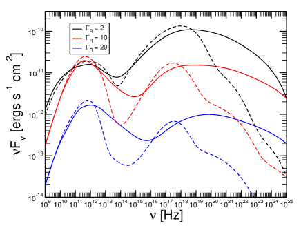
Figure 8: Averaged spectra for weakly magnetized shells with varying slower shell bulk Lorentz factor, $\Gamma_{\rm R}$, and two different non-thermal particles fractions: $\zeta_{\rm e}=0.9,0.1$, solid and dashed lines respectively.

6.5 Total luminosity

The number of particles accelerated by the internal shocks is an important quantity in our treatment of EEDs. The number of particles in each shell is dictated by Eq. (1). Such a direct influence of the luminosity on the number of particles motivates us to study the behaviour of the SEDs when this parameter is changed. In Fig. 9 we show the SEDs produced by the IS model with different total jet luminosities and values of $\zeta_{\rm e}$ (models W-G10-D1.0-Z(09, m1)-$\boldsymbol{\mathcal{L}}$(1, 5, 50)). With solid and dashed lines we differentiate the HDs with $\zeta_{\rm e}=0.9,0.1$, respectively, and in black, red and blue the luminosities $\boldsymbol{\mathcal{L}}=10^{47},5\times 10^{47},5\times 10^{48}$, respectively. The increase in flux of the thermally or non-thermally dominated cases is rather similar, and follows the expectations. An increase by 50 in the total luminosity $\boldsymbol{\mathcal{L}}$ implies an overall increase of 100 in the particle density according to Eq. (1). Hence, the expected increase in flux in the synchrotron component is proportional to $n_{i}\sim 100$, while in the SSC component it is proportional to $n_{i}^{2}\sim 10^{4}$.

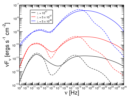
Figure 9: Averaged spectra for different jet total luminosity. Solid and dashed lines display the models with $\zeta_{\rm e}=0.9,0.1$, respectively. Different color lines correspond to different values of the jet luminosity (see legend).

7 Temperature vs. magnetization

The fluid temperature $\chi$ is calculated by the exact Riemann solver for each shell collision. Assuming that the jet is composed of protons and electrons, the temperature of the electrons in the plasma is $\Theta_{\rm e}=\chi m_{\rm p}/m_{\rm e}$, where $m_{\rm p}$ is the proton mass. In order to systematically explore the dependence of the temperature on the properties of the shells we solved a large number of Riemann problems for different magnetizations and relative Lorentz factor. Here we present the behaviour of $\Theta_{\rm e}$ in the ISs model in order to obtain insight into the temperature of the thermal component of the EED in the shocks. In Fig. 10 we show the value of $\Theta_{\rm e}$ as a function of the magnetizations $\sigma_{\rm L}\mbox{ and }\sigma_{\rm R}$ for both FS and RS (left and right panels, respectively).

The hottest region of the RS plane ($\sigma_{\rm L}<1$ and $\sigma_{\rm R}>0.1$) corresponds to the coldest region in the FS plane. Indeed, comparing both figures we observe that the RS is hotter than the FS wherever $\sigma_{\rm L}\lesssim 0.2$ or $\sigma_{\rm R}>0.1$. As a result, in most of the moderately and weakly magnetized models, the radiation produced by the population of injected electrons that are thermally dominated could come from the RS. However, for $\sigma_{\rm R}\lesssim 0.2$ and $\sigma_{\rm L}\gtrsim 0.2$ the oposite true: the FS is hotter than the RS.

Figure 10: Dependence of the electron temperature on shell magnetization. The top and bottom panels show the behaviour of $\Theta_{\rm e}$ in the FS and RS, respectively. Contour lines of selected temperatures are overlaid in both panels.

In Fig. 11 we show the behavior of the electron temperature $\Theta_{\rm e}$ in terms of the relative Lorentz factor $\Delta g$ between the colliding shells for the FS and RS. In accordance with figures 10, the reverse shock is hotter than the forward shock. As the relative Lorentz factor $\Delta g$ grows the temperature of the reverse shock tends to grow while the forward shock seems to be approaching asymptotically to a value, which depends slightly on the magnetization (the larger the magnetization the smaller the asymptotic temperature). Values $\Delta g>5$ are inconsistent with the blazar scenario, for a fixed value $\Gamma_{\rm R}=10$, since they would imply that the faster shell was moving at $\Gamma_{\rm L}>60$ (in excess of the maximum values of the Lorentz factor for the bulk motion inferred for blazars).

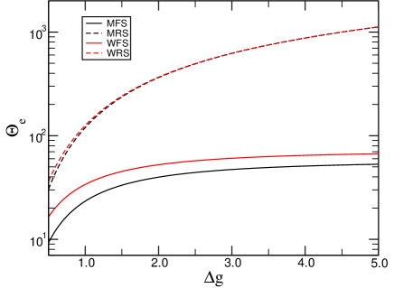
Figure 11: Temperature as a function of the relative Lorentz factor. In this figure we show the temperature of both forward (full lines) and reverse (dashed lines) shocks for the weakly (red lines) and moderately (black lines) magnetized models. The value of the bulk Lorentz factor of the slower shell for both magnetization is $\Gamma_{\rm R}=10$.

From figures 10 and 11 we can infer that $\Theta_{\rm e}$ does not only depend on the velocity of the fluid but also on its magnetization. Therefore, we conclude that this degeneracy makes the determination of $\Theta_{e}$ a very difficult task.

8 Discussion and conclusions

In this work we introduce a hybrid thermal-non-thermal electron distribution into the internal shock model for blazars. To account for the fact that the thermal component of the HD extends to very low electron Lorentz factors, we also introduce a cyclo-synchrotron code that enables us to compute the non-thermal emission from electrons with arbitrary Lorentz factor. We show that our method for treating the temporal evolution of the HD and the calculation of MBS emission can be performed efficiently and with sufficient accuracy. The method is implemented as a generalization of the numerical code of MA12.

To test the influence of the fraction of non-thermal particles $\zeta_{\rm e}$ in the overall HD we apply the new method to the case of a blazar with $\boldsymbol{\mathcal{L}}=10^{47}\,\mathrm{erg}\,\mathrm{s}^{-1}$ (Fig. 5). Considering only MBS and SSC emission processes we see that increasing $\zeta_{\rm e}$ (i.e., the distribution becoming more non-thermal) has as a consequence a shallower valley between the two spectral peaks, while the SSC emission extends to higher energies. In other words, a HD of mostly thermal particles emits only up to MeV (except when $\Delta g\sim 5$; see Fig. 7). This would mean that the emission in the GeV range for the thermally-dominated HD cannot come from the SSC and would have to be produced by the EIC (not considered here). Furthermore, Fig. 5 confirms that also for low $\zeta_{\rm e}$ highly-magnetized blazar jets seem to be observationally excluded because their SSC peak is too dim.

Another effect of decreasing $\zeta_{\rm e}$ is the shift of the SSC peak to lower frequencies and the narrowing of the high-frequency spectral bump, while at the same time the synchrotron peak and flux do not change appreciably. This means that (excluding possible effects from varying EIC) the Compton dominance (ratio of internal Compton and cyclosynchrotron luminosity) can be changed by varying $\zeta_{\rm e}$, while the peak MBS frequency remains constant. In other words, for all other parameters remaining constant, the variations in $\zeta_{\rm e}$ may explain the vertical scatter in the distribution of FSRQs and BL Lacs in the peak synchrotron frequency- Compton dominance parameter space (see e.g., Fig. 5 in Finke, 2013). Changing $\zeta_{\rm e}$ appears to not be able to change the blazar class.

Regarding the variations of the shell magnetization (Sec. 6.2), relative Lorentz factor (Sec. 6.3) and the bulk Lorentz factor (Sec. 6.4), the results are consistent with those of RMA14. In this work we performed a more detailed study of the influence of the magnetization than in the previous paper since now we study $9$ possible combinations of faster and slower shell magnetizations, instead of only three in RMA14. The truly novel result of this work is that the RMA14 trend generally holds for the thermally-dominated HD as well (right panel in Fig. 6), with the difference that the collision of $(\sigma_{\rm L}=0.1,\sigma_{\rm R}=0.1)$ shells produces a double-peaked spectrum for $\zeta_{e}=0.1$, while its non-thermally dominated equivalent does not (blue dashed lines in Fig. 6). Even so, the SSC component remains very dim for very magnetized shells.

Regarding $\Delta g$, the RS emission (dot-dashed lines in Fig. 7) is crucial for reproducing the blazar spectrum. Therefore, in the case of $\zeta_{e}\ll 1$ the temperature of the RS is one of the most important parameters. Since this temperature increases with $\Delta g$ (Fig. 11), the effect of $\Delta g$ on the MBS and the SSC peak frequencies and fluxes is qualitatively similar to that of the non-thermal electron distribution (Fig. 7; see also RMA14). The changes induced by variations of $\Gamma_{\rm R}$ (Fig. 8) are independent of the thermal/non-thermal EED content and agree with RMA14. The effects of the increase in total jet luminosity are visible both for $\zeta_{\rm e}=0.1$ and $\zeta_{\rm e}=0.9$. Varying the luminosity by a factor $50$ increases the MBS flux by $\sim 10^{2}$ and the SSC flux by $\sim 10^{4}$. The relation between spectral components is very similar to the variations of $\Gamma_{\rm R}$, i.e. the increase in ${\cal L}$ is similar to a decrease in $\Gamma_{\rm R}$.

Overall, we show that the inclusion of the full cyclo-synchrotron treatment, motivated by the significant low-energy component of the HD, has a moderate effect on the blazar spectrum at optical-to-$\gamma$ ray frequencies. However, at lower frequencies (e.g., below 1 GHz) where the self-absorption may play a role the differences between the synchrotron and the MBS will be more severe. We plan to include the effect of absorption in a future work as well as the effects by EIC emission.

Appendix A The RMA function

The formula for the pitch-angle averaged synchrotron power of a single ultrarelativistic electron was derived in e.g., Crusius & Schlickeiser (1986) and afterwards, an accurate approximation of it was discovered by Schlickeiser & Lerche (2007). Both expressions assume a continuum spectrum for all $\gamma$, so that they cannot be applied directly to the calculation of the discrete low-frequency, low-$\gamma$ cyclotron emission. In particular, these formulae do not take into account the fact that for slow electrons there is no emission below the gyrofrequency $\nu_{b}$. Nevertheless, the expression in Schlickeiser & Lerche (2007) is analytic, which makes it very convenient for a fast numerical implementation. We use the Eq. (16) in Schlickeiser & Lerche (2007) to define the function

$$RMA[x]:=\begin{cases}x\,CS[x]&x>2a/(3\gamma^{3})\\ 0&\text{otherwise}\end{cases},$$ (43)

where $a$ is a numerical constant. The location of the cut-off; i.e., the value of $a$ in Eq. (43), is very important. In Fig. 12 we show the relative error of the emissivity using $RMA[x]$ compared to full MBS treatment. We assume a pure power-law distribution of electrons with different power-law indices and use two different values of the cut-off constant: $a=0.8$ and $a=1$. The magnetic field for this test was $B=10\,\mathrm{G}$ and the minimum and maximum Lorentz factors $\gamma_{\rm min}^{\rm nth}=5,\gamma_{\rm max}^{\rm nth}=500$, respectively. At low frequencies the errors are large because there the emission is dominated by harmonics and is thus not well represented by a continuous $RMA[x]$ function. Nevertheless, choosing an appropriate value for $a$ can decrease the errors in that region from $\sim 350$% ($a=1$, right panel) to $\sim 25$% ($a=0.8$, left panel). The relative error of the cases with power-law indices $q<0$ are always below 1, and is somewhat lower for $a=1$ than for $a=0.8$. However, since we want the relative error to be the lowest for all power-law indices, we choose the cut-off constant $a=0.8$.

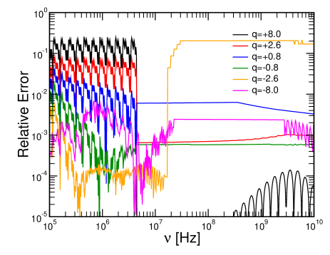
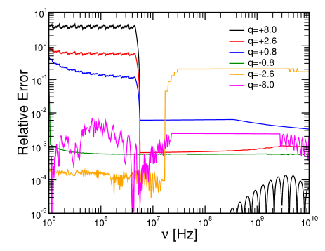
Figure 12: The relative error between emissivity for a power-law distribution of electrons computed from the MBS interpolation tables and performing numerical integration of the RMA function. Each of the different colours represent cases with different power-law indices, $q$, of the non-thermal EED. In the left and right panels we show the relative error considering $a=0.8$ and $a=1$ in Eq. 43, respectively.

Appendix B The ${\cal X}^{2}I_{1}$X_2 I_1 interpolation table

The interpolation table of $\tilde{I}_{1}(\gamma,{\cal X}):={\cal X}^{2}I_{1}({\cal X},\gamma)$ was built integrating Eq. (30) using the Gauss-Legendre quadrature with 120 nodal points for values of $\gamma\leq\gamma_{\rm up}$ and ${\cal X}\leq 10^{2}$. For ${\cal X}>10^{2}$ and $\gamma>\gamma_{\rm up}$ we employ the approximate expression $\tilde{I}_{1}(\gamma,{\cal X})\simeq RMA[x]$ (see Eq. (37)). The numerical calculations of the Bessel functions were performed using the tool my_Bessel_J developed in Leung et al. (2011). Computing $\tilde{I}_{1}(\gamma,{\cal X})$ for $\gamma$ and ${\cal X}$ outside this region is computationally challenging. Fortunately, in the ultrarelativistic regime we can approximate $\tilde{I}_{1}(\gamma,{\cal X})$ using the $RMA$ function (see App. A). In the $\gamma$ direction $\tilde{I}_{1}$ is approximated using Chebyshev interpolation (for each ${\cal X}$ separately).

Figure 13: ${\cal X}^{2}I_{1}$ as a function of ${\cal X}$ and $\gamma$. The emission is zero in the light blue region. We also note that for arbitrary $\gamma$ there is a sufficiently low ${\cal X}$ so that the emission is in the form of harmonics.

Special care has to be devoted to the zero emission regions below ${\cal X}_{1}(\gamma)$ and above ${\cal X}=100$ (light blue triangular zones in Fig. 13), since including those regions can cause a bad numerical behaviour of Chebyshev interpolation. In order to avoid this, we constructed a Lorentz factors array $\{\hat{\gamma}_{\min}({\cal X})\}$ containing the minimum Lorentz factor above which the emission is non-negligible for every value of ${\cal X}$; i.e., $\{\hat{\gamma}_{\min}({\cal X})\}$ is a set of lower interval limits for the Chebyshev interpolation (instead of $\gamma=1$).

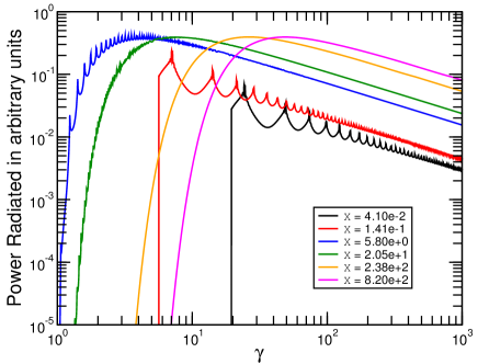
Figure 14: Similar to Fig. 1 but for a fixed ${\cal X}$. The black and red lines depict the radiated power for ${\cal X}<{\cal X}_{1}$. The break at low $\gamma$ is set by hand considering the cut-off criteria described in Sec. A. The blue and green lines correspond to ${\cal X}_{1}\leq{\cal X}<100$. The orange and magenta lines correspond to ${\cal X}\geq 100$.

B.1 Minimum Lorentz factors for ${\cal X}<{\cal X}_{1}$X ¡ X1

Numerical calculations of the cyclo-synchrotron radiated power show that the frequency of the first harmonic behaves as ${\cal X}_{1}(\gamma)=1/\gamma$. In App. A we show the cut-off criterion chosen to include as much power radiated as possible while avoiding the zero emission frequencies below ${\cal X}_{1}(\gamma)$. We follow a similar procedure to construct the array $\{\hat{\gamma}_{\min}({\cal X})\}$; i.e., $\hat{\gamma}_{\min}({\cal X})=0.8/{\cal X}$.

B.2 Minimum Lorentz factors for ${\cal X}\geq 100$X ¿= 100

Finding $\hat{\gamma}_{\min}({\cal X})$ for this side of the spectrum requires of a two-step procedure:

1. For every ${\cal X}$ the bisection method was employed to find the value of $\gamma$ at which $\tilde{I}_{1}$ is well below its maximum value.

2. A linear fit (in logarithmic space) was performed with the values of $\gamma$ found in the previous step.

We used the formula obtained from the fit to estimate the values of $\hat{\gamma}_{\min}({\cal X})$ in this region.

B.3 Minimum Lorentz factors for ${\cal X}_{1}\leq{\cal X}<100$X_1 ¡= 100

Our calculations showed that in the region where $1\leq{\cal X}<100$ there is practically no zero radiation region in the $\gamma$ direction (see Fig. 13). Since this region is above the first harmonic ${\cal X}_{1}$, neither the criterion used in App. B.1 nor the bisection procedure employed in App. B.2 can be used here since the profile of $\tilde{I}_{1}$ is too steep at $\gamma\sim 1$ (see Fig. 14). Applying a bisection method leads to an oscillating $\hat{\gamma}_{\min}({\cal X})$ which, produces numerical problems when interpolating from the table. We verified that a constant Lorentz factor minimum threshold close to 1 produces good results in this region. Thus, we employ the input parameter $\gamma_{\rm min}^{\rm th}$ for this purpose. Normally we use the numerical value $\gamma_{\rm min}^{\rm th}\approx 1.005037815$ which corresponds to the Lorentz factor of a particle with $\beta=0.1$. The exact value $\gamma=1$ cannot be used as threshold because it corresponds to $\beta=0$, causing problems in e.g., the resonance condition (Eq. (24)) and the subsequent equations.

B.4 Calculation of ${\cal X}^{2}I_{1}({\cal X},\gamma)$X2 I1(X, g) using the interpolation table

The usage of $\tilde{I}_{1}$ requires a two-step procedure: (1) Chebyshev interpolation from the Chebyshev coefficients in the $\gamma$ direction and (2) a linear interpolation in the ${\cal X}$ direction using the values obtained in the first step. The accuracy of the reconstruction routine can be seen in Fig. 15. The test was performed on a grid of $1024\times 1024$. The relative error in most of the points is $\lesssim 1$%.

Figure 15: Similar to Fig. 13, but showing the relative error between the data obtained using numerical integration and the values interpolated from the table. The resolution of the plot is $1024\times 1024$ points.

References

- Aloy & Mimica (2008) Aloy M. A., Mimica P., 2008, \hrefhttp://dx.doi.org/10.1086/588605 ApJ, \hrefhttp://adsabs.harvard.edu/abs/2008ApJ…681…84A 681, 84
- Asada & Nakamura (2012) Asada K., Nakamura M., 2012, \hrefhttp://dx.doi.org/10.1088/2041-8205/745/2/L28 ApJL, \hrefhttp://adsabs.harvard.edu/abs/2012ApJ…745L..28A 745, L28
- Bekefi (1966) Bekefi G., 1966, Radiation processes in plasmas. Wiley series in plasma physics, Wiley
- Beskin & Nokhrina (2006) Beskin V. S., Nokhrina E. E., 2006, \hrefhttp://dx.doi.org/10.1111/j.1365-2966.2006.09957.x MNRAS, \hrefhttp://adsabs.harvard.edu/abs/2006MNRAS.367..375B 367, 375
- Blandford & Rees (1974) Blandford R. D., Rees M. J., 1974, \hrefhttp://dx.doi.org/10.1093/mnras/169.3.395 MNRAS, \hrefhttp://adsabs.harvard.edu/abs/1974MNRAS.169..395B 169, 395
- Boettcher (2010) Boettcher M., 2010, preprint (\hrefhttp://arxiv.org/abs/1006.5048 arXiv:1006.5048)
- Böttcher & Dermer (2002) Böttcher M., Dermer C. D., 2002, \hrefhttp://dx.doi.org/10.1086/324134 ApJ, \hrefhttp://adsabs.harvard.edu/abs/2002ApJ…564…86B 564, 86
- Böttcher & Dermer (2010) Böttcher M., Dermer C. D., 2010, \hrefhttp://dx.doi.org/10.1088/0004-637X/711/1/445 ApJ, \hrefhttp://adsabs.harvard.edu/abs/2010ApJ…711..445B 711, 445
- Chandrasekhar (1939) Chandrasekhar S., 1939, An introduction to the study of stellar structure; 1st ed.. Dover books on advanced mathematics, Dover, New York, NY
- Crusius & Schlickeiser (1986) Crusius A., Schlickeiser R., 1986, A&A, 164, L16
- Finke (2013) Finke J. D., 2013, \hrefhttp://dx.doi.org/10.1088/0004-637X/763/2/134 ApJ, \hrefhttp://adsabs.harvard.edu/abs/2013ApJ…763..134F 763, 134
- Finke et al. (2008) Finke J. D., Dermer C. D., Böttcher M., 2008, \hrefhttp://dx.doi.org/10.1086/590900 ApJ, 686, 181
- Fossati et al. (1998) Fossati G., Maraschi L., Celotti A., Comastri A., Ghisellini G., 1998, \hrefhttp://dx.doi.org/10.1046/j.1365-8711.1998.01828.x MNRAS, \hrefhttp://cdsads.u-strasbg.fr/abs/1998MNRAS.299..433F 299, 433
- Ghisellini et al. (1998) Ghisellini G., Celotti A., Fossati G., Maraschi L., Comastri A., 1998, \hrefhttp://dx.doi.org/10.1046/j.1365-8711.1998.02032.x MNRAS, \hrefhttp://cdsads.u-strasbg.fr/abs/1998MNRAS.301..451G 301, 451
- Giannios & Spitkovsky (2009) Giannios D., Spitkovsky A., 2009, \hrefhttp://dx.doi.org/10.1111/j.1365-2966.2009.15454.x MNRAS, \hrefhttp://adsabs.harvard.edu/abs/2009MNRAS.400..330G 400, 330
- Ginzburg & Syrovatskii (1965) Ginzburg V. L., Syrovatskii S. I., 1965, \hrefhttp://dx.doi.org/10.1146/annurev.aa.03.090165.001501 ARA&A, \hrefhttp://adsabs.harvard.edu/abs/1965ARA
- Giommi et al. (2012) Giommi P., Padovani P., Polenta G., Turriziani S., D’Elia V., Piranomonte S., 2012, \hrefhttp://dx.doi.org/10.1111/j.1365-2966.2011.20044.x MNRAS, \hrefhttp://adsabs.harvard.edu/abs/2012MNRAS.420.2899G 420, 2899
- Giommi et al. (2013) Giommi P., Padovani P., Polenta G., 2013, \hrefhttp://dx.doi.org/10.1093/mnras/stt305 MNRAS, \hrefhttp://adsabs.harvard.edu/abs/2013MNRAS.431.1914G 431, 1914
- Joshi & Böttcher (2011) Joshi M., Böttcher M., 2011, ApJ, 727, 21
- Kardashev (1962) Kardashev N. S., 1962, SvA, \hrefhttp://adsabs.harvard.edu/abs/1962SvA…..6..317K 6, 317
- Königl (1981) Königl A., 1981, \hrefhttp://dx.doi.org/10.1086/158638 ApJ, \hrefhttp://adsabs.harvard.edu/abs/1981ApJ…243..700K 243, 700
- Krawczynski & Treister (2013) Krawczynski H., Treister E., 2013, \hrefhttp://dx.doi.org/10.1007/s11467-013-0310-3 Frontiers of Physics, \hrefhttp://adsabs.harvard.edu/abs/2013FrPhy…8..609K 8, 609
- Krichbaum et al. (2006) Krichbaum T. P., Agudo I., Bach U., Witzel A., Zensus J. A., 2006, in Proceedings of the 8th European VLBI Network Symposium. p. 2 (\hrefhttp://arxiv.org/abs/astro-ph/0611288 arXiv:astro-ph/0611288)
- Leung et al. (2011) Leung P. K., Gammie C. F., Noble S. C., 2011, \hrefhttp://dx.doi.org/10.1088/0004-637X/737/1/21 ApJ, \hrefhttp://adsabs.harvard.edu/abs/2011ApJ…737…21L 737, 21
- Li et al. (1996) Li H., Kusunose M., Liang E. P., 1996, \hrefhttp://dx.doi.org/10.1086/309960 ApJL, \hrefhttp://adsabs.harvard.edu/abs/1996ApJ…460L..29L 460, L29
- Lister et al. (2016) Lister M. L., et al., 2016, \hrefhttp://dx.doi.org/10.3847/0004-6256/152/1/12 AJ, \hrefhttp://adsabs.harvard.edu/abs/2016AJ….152…12L 152, 12
- McKinney (2006) McKinney J. C., 2006, \hrefhttp://dx.doi.org/10.1111/j.1365-2966.2006.10256.x MNRAS, \hrefhttp://adsabs.harvard.edu/abs/2006MNRAS.368.1561M 368, 1561
- Melrose & McPhedran (1991) Melrose D. B., McPhedran R. C., 1991, Electromagnetic Processes in Dispersive Media. Cambridge University Press, Cambridge
- Mimica (2004) Mimica P., 2004, PhD thesis, Max-Planck-Institut für Astrophysik
- Mimica & Aloy (2010) Mimica P., Aloy M. A., 2010, MNRAS, 401, 525
- Mimica & Aloy (2012) Mimica P., Aloy M. A., 2012, \hrefhttp://dx.doi.org/10.1111/j.1365-2966.2012.20495.x MNRAS, 421, 2635
- Mimica et al. (2004) Mimica P., Aloy M. A., Müller E., Brinkmann W., 2004, A&A, 418, 947
- Mimica et al. (2007) Mimica P., Aloy M. A., Müller E., 2007, A&A, 466, 93
- Mimica et al. (2009) Mimica P., Aloy M. A., Agudo I., Marti J. M., Gómez J.-L., Miralles J. A., 2009, ApJ, 696, 1142
- Mimica et al. (2010) Mimica P., Giannios D., Aloy M. A., 2010, MNRAS, 407, 2501
- Mohan et al. (2015) Mohan P., et al., 2015, \hrefhttp://dx.doi.org/10.1093/mnras/stv1412 MNRAS, \hrefhttp://adsabs.harvard.edu/abs/2015MNRAS.452.2004M 452, 2004
- Nakamura & Asada (2013) Nakamura M., Asada K., 2013, \hrefhttp://dx.doi.org/10.1088/0004-637X/775/2/118 ApJ, \hrefhttp://adsabs.harvard.edu/abs/2013ApJ…775..118N 775, 118
- Oster (1961) Oster L., 1961, \hrefhttp://dx.doi.org/10.1103/PhysRev.121.961 Physical Review, \hrefhttp://adsabs.harvard.edu/abs/1961PhRv..121..961O 121, 961
- Pacholczyk (1970) Pacholczyk A. G., 1970, Radio astrophysics. Nonthermal processes in galactic and extragalactic sources. Series of Books in Astronomy and Astrophysics, Freeman, San Francisco
- Petrosian (1981) Petrosian V., 1981, \hrefhttp://dx.doi.org/10.1086/159517 ApJ, \hrefhttp://adsabs.harvard.edu/abs/1981ApJ…251..727P 251, 727
- Rees & Meszaros (1994) Rees M. J., Meszaros P., 1994, ApJL, 430, L93
- Romero et al. (2005) Romero R., Marti J., Pons J. A., Ibáñez J. M., Miralles J. A., 2005, JFM, 544, 323
- Rueda-Becerril et al. (2014) Rueda-Becerril J. M., Mimica P., Aloy M. A., 2014, \hrefhttp://dx.doi.org/10.1093/mnras/stt2335 MNRAS, \hrefhttp://adsabs.harvard.edu/abs/2014MNRAS.438.1856R 438, 1856
- Rybicki & Lightman (1979) Rybicki G. B., Lightman A. P., 1979, Radiative processes in astrophysics. Wiley-Interscience, New York
- Schlickeiser & Lerche (2007) Schlickeiser R., Lerche I., 2007, \hrefhttp://dx.doi.org/10.1051/0004-6361:20078088 A&A, 476, 1
- Sironi et al. (2013) Sironi L., Spitkovsky A., Arons J., 2013, \hrefhttp://dx.doi.org/10.1088/0004-637X/771/1/54 ApJ, \hrefhttp://adsabs.harvard.edu/abs/2013ApJ…771…54S 771, 54
- Spada et al. (2001) Spada M., Ghisellini G., Lazzati D., Celotti A., 2001, MNRAS, 325, 1559
- Urry & Padovani (1995) Urry C. M., Padovani P., 1995, \hrefhttp://dx.doi.org/10.1086/133630 PASP, \hrefhttp://adsabs.harvard.edu/abs/1995PASP..107..803U 107, 803
- Zacharias & Schlickeiser (2010) Zacharias M., Schlickeiser R., 2010, \hrefhttp://dx.doi.org/10.1051/0004-6361/201015284 A&A, 524, A31
- Zdziarski et al. (1990) Zdziarski A. A., Coppi P. S., Lamb D. Q., 1990, \hrefhttp://dx.doi.org/10.1086/168901 ApJ, \hrefhttp://adsabs.harvard.edu/abs/1990ApJ…357..149Z 357, 149