Prospect for observing a light charged Higgs through the decay $H^{+}\to c\bar{b}+c.c.$ at the LHeC

Abstract:

We study the production and decay of a light charged Higgs boson at the future Large Hadron electron Collider (LHeC) in the framework of the Two Higgs Doublet Type III, assuming a four-zero texture in the Yukawa matrices and a general Higgs potential. We analyze the charge current production processes $e^{-}p\to\nu_{e}qH^{+}$ considering the signature $H^{+}\to c\bar{b}+c.c.$ of the final state. We take this signature and we compare it to the irreducible background from Standard Model (SM) interactions. We consider scenarios of the model which are consistent with current experimental data from Higgs and flavor physics.

1 Introduction

Once discovered, a neutral Higgs boson at the Large Hadron Collider (LHC), by the ATLAS [1] and CMS [2] experiments, the SM is well established. However, the SM-like limit exists for several extensions of the Higgs sector, e.g., the 2-Higgs Doublet Model (2HDM) in its versions Type I, II, III (or Y) and IV (or X), wherein Flavor Changing Neutral Currents (FCNCs) mediated by (pseudo)scalars can be eliminated under discrete symmetries [3]. Another, very interesting kind of 2HDM is the one where FCFNs can be controlled by a particular texture in the Yukawa matrices [3]. In particular, we have implemented a four zero-texture in a scenario which we have called 2HDM Type III (2HDM-III). This model has a phenomenology which is very rich, which we studied at colliders some years ago [4, 5], and some very interesting aspects, like flavor-violating quarks decays $\phi\to b\bar{s}$ ($\phi=h,\,H$), which can be enhanced for neutral Higgs bosons with intermediate mass (i.e., below the top quark mass) [6]. Similarly, in this model, the parameter space can avoid the current experimental constraints of flavor and Higgs physics and a light charged Higgs boson is allowed [4], so that the decay $H^{+}\to c\bar{b}$ is enhanced and its Branching Ratio ($BR$) could be dominant. In fact, this channel has been also studied in a variety of Multi-Higgs Doublet Models (MHDMs) [7, 8], wherein the $BR(H^{+}\to c\bar{b})\approx 0.7-0.8$ and could afford one with a considerable gain in sensitivity to the presence of a $H^{\pm}$ by tagging the $b$ quark. In this work, we focus on the feasibility of finding at the future LHeC the charged Higgs boson of the 2HDM-III.

2 The Higgs-Yukawa sector in the 2HDM-III

As we have shown previously, in the 2HDM-II, when the four-zero-texture is implemented and FCNCs are controlled, the discrete symmetry in the model is not necessary. Then the most general $SU(2)_{L}\times U(1)_{Y}$ invariant scalar potential for two scalar doublets, $\Phi_{i}^{\dagger}=(\phi_{i}^{-},\phi_{i}^{0*})$ ($i=1,\,2$), must be considered, which is:

$$V(\Phi_{1},\Phi_{2}) = \mu_{1}^{2}(\Phi_{1}^{\dagger}\Phi_{1})+\mu_{2}^{2}(\Phi_{2}^{\dagger}\Phi_{2})-\Big{(}\mu_{12}^{2}(\Phi_{1}^{\dagger}\Phi_{2})+h.c.\Big{)}+\frac{1}{2}\lambda_{1}(\Phi_{1}^{\dagger}\Phi_{1})^{2}+\frac{1}{2}\lambda_{2}(\Phi_{2}^{\dagger}\Phi_{2})^{2}$$ (1)

$$+\lambda_{3}(\Phi_{1}^{\dagger}\Phi_{1})(\Phi_{2}^{\dagger}\Phi_{2})+\lambda_{4}(\Phi_{1}^{\dagger}\Phi_{2})(\Phi_{2}^{\dagger}\Phi_{1})+\left[\frac{1}{2}\lambda_{5}(\Phi_{1}^{\dagger}\Phi_{2})^{2}+\Big{(}\lambda_{6}(\Phi_{1}^{\dagger}\Phi_{1})\right.$$

$$\left.+\lambda_{7}(\Phi_{2}^{\dagger}\Phi_{2})\Big{)}(\Phi_{1}^{\dagger}\Phi_{2})+h.c.\right],$$

where all parameters of the Higgs potential are assumed to be real, including the Vacuum Expectation Values (VEVs) of the scalar fields (i.e., the CP violation case is not considered). Hence, in the 2HDM-III, both doublets are coupled with the same fermions, so the Yukawa Lagrangian is given by:

$${\cal L}_{Y}=-\Big{(}Y_{1}^{u}\bar{Q}_{L}\tilde{\Phi}_{1}u_{R}+Y_{2}^{u}\bar{Q}_{L}\tilde{\Phi}_{2}u_{R}+Y_{1}^{d}\bar{Q}_{L}\Phi_{1}d_{R}+Y_{2}^{d}\bar{Q}_{L}\Phi_{2}d_{R}+Y_{1}^{l}\bar{L}\Phi_{1}l_{R}+Y_{2}^{l}\bar{L}_{L}\Phi_{2}l_{R}\Big{)},$$ (2)

where $\tilde{\Phi}_{1,2}=i\sigma_{2}\Phi_{1,2}^{*}$. Since, in this equation, the fermion mass matrices after Electro-Weak Symmetry Breaking (EWSB) are expressed by: $M_{f}=\frac{1}{2}(v_{1}Y_{1}^{f}+v_{2}Y_{2}^{f})$, $f=u,\,d,\,l$, assuming that both Yukawa matrices $Y_{1}$ and $Y_{2}$ have the four zero-texture form and are Hermitian [9]. Once we diagonalize the mass matrices, one can get the rotated matrix $Y_{n}^{f}$ with the following generic expression:

$$[\tilde{Y}_{n}^{f}]_{ij}=\frac{\sqrt{m_{i}^{f}m_{j}^{f}}}{v}[\tilde{\chi}_{n}^{f}]_{ij}=\frac{\sqrt{m_{i}^{f}m_{j}^{f}}}{v}[\chi_{n}^{f}]_{ij}e^{i\theta_{ij}^{f}},$$ (3)

where the $\chi^{\prime}s$ are unknown dimensionless parameters of the model, with $v=\sqrt{v_{1}^{2}+v_{2}^{2}}$. Following the procedure of Ref. [4], we can obtain a generic expression for the couplings of the Higgs bosons with the fermions, by means of

$${\cal L}^{\bar{f}_{i}f_{j}\phi} = -\left\{\frac{\sqrt{2}}{v}\bar{u}_{i}(m_{d_{j}}X_{ij}P_{R}+m_{u_{i}}Y_{ij}P_{l})d_{j}H^{+}+\frac{\sqrt{2}m_{l_{j}}}{v}Z_{ij}\bar{v_{L}}l_{R}H^{+}+h.c.\right\}$$ (4)

$$-\frac{1}{v}\Big{\{}\bar{f}_{i}m_{f_{i}}h_{ij}^{f}f_{j}h^{0}+\bar{f}_{i}m_{f_{i}}H_{ij}^{f}f_{j}H^{0}-i\bar{f}_{i}m_{f_{i}}A_{ij}^{f}f_{j}\gamma_{5}A^{0}\Big{\}},$$

where $\phi_{ij}^{f}$ ($\phi=h$, $H$, $A$), $X_{ij}$, $Y_{ij}$, $Z_{ij}$ are defined in [4], a structure that can be related to various incarnations of the 2HDM with additional flavor physics in the Yukawa matrices, in such a way that the Higgs-fermion-antifermion coupling can be written as $g^{\phi ff}_{\rm 2HDM-III}=g^{\phi ff}_{\rm 2HDM-any}+\Delta g$, where $g^{\phi ff}_{\rm 2HDM-any}$ is the coupling $\phi f\bar{f}$ in 2HDMs with a $Z_{2}$ discrete symmetry and $\Delta g$ is the contribution of the four-zero texture.

Now, we consider three different realisations of the 2HDM-III, which give an enhancement to the decay channel $H^{+}\to c\bar{b}+h.c.$, in fact, this $BR$ could be the leading one.

3 Benchmark scenarios of the 2HDM-III

We perform a parameter scan of the 2HDM-III similar to that of Ref. [6], where all recent experimental bounds from flavor and Higgs physics (including EW Precision Observables (EWPOs)) were taken into account, alongside perturbativity, vacuum stability and unitarity constraints [4, 10]. Then, we choose the same benchmark scenarios given in [6], because in these cases the charged Higgs mass is light (110 GeV $\leq m_{H^{\pm}}\leq 200$ GeV). From the parameter space that survives current theoretical requirements and experimental data, we take the points that present a substantial enhancement of the decay $H^{+}\to c\bar{b}+h.c.$, whose $BR(H^{+}\to c\bar{b}+h.c.)\approx 1$. Thus, the following benchkmark scenarios are considered:

• Scenario Ia: $\cos(\beta-\alpha)=0.1$, $\chi^{u}_{kk}=1.5$ ($k=2$, 3), $\chi_{22}^{d}=1.8$, $\chi_{33}^{d}=1.2$, $\chi_{23}^{u,d}=0.2$, $\chi_{22}^{\ell}=0.5$, $\chi_{33}^{\ell}=1.2$, $\chi_{23}^{\ell}=0.1$, $M_{A}=100$ GeV, $m_{H^{\pm}}=$ 110 GeV, taking $Y=-X=-Z=\cot\beta$.

• Scenario Ib: the same of Scenario Ia, but with $\cos(\beta-\alpha)=0.5$.

• Scenario IIa: $\cos(\beta-\alpha)=0.1$, $\chi^{u}_{22}=0.5$, $\chi^{u}_{33}=1.4$, $\chi_{22}^{d}=2$, $\chi_{33}^{d}=1.3$, $\chi_{23}^{u}=-0.53$, $\chi_{23}^{d}=0.2$, $\chi_{22}^{\ell}=0.4$, $\chi_{33}^{\ell}=1.2$, $\chi_{23}^{\ell}=0.1$, $M_{A}=100$ GeV, $m_{H^{\pm}}=$ 110 GeV, taking $X=Z=\tan\beta=1/Y$.

• Scenario Ya: $\cos(\beta-\alpha)=0.1$, $\chi^{u}_{22}=0.5$, $\chi^{u}_{33}=1.4$, $\chi_{22}^{d}=2$, $\chi_{33}^{d}=1.3$, $\chi_{23}^{u}=-0.53$, $\chi_{23}^{d}=0.2$, $\chi_{22}^{\ell}=0.4$, $\chi_{33}^{\ell}=1.1$, $\chi_{23}^{\ell}=0.1$, $M_{A}=100$ GeV, $m_{H^{\pm}}=$ 110 GeV, taking $X=1/Y=\tan\beta=-1/Z$.

4 Numerical analysis

We study the process $e^{-}p\to\nu_{e}H^{-}b$ proceeding via two subprocesses: $e^{-}\bar{b}\to\nu_{e}\bar{t}\to\nu_{e}H^{-}\bar{b}$ (single top quark production and decay) and $e^{-}\bar{b}\to\nu_{e}W^{\pm*}\phi^{*}\to\nu_{e}H^{-}\bar{b}$ (vector-scalar fusion) [11]. We assume that $H^{-}\to\bar{c}b$ is dominant. Our signal contains three jets (one is forward and two are central), missing transverse energy and no lepton. Out of the two central jets, one is $b$-tagged. We estimate the parton level signal cross section and $BR(H^{+}\to c\bar{b}+h.c.)$ using CalcHEP [12]. For this study at the LHeC, we consider an electron beam with energy $E_{e^{-}}=60$ GeV while the energy of the proton beam is $E_{p}=7000$ GeV, which correspond to a center-of mass energy $\sqrt{s}=1.3$ TeV. The integrated luminosity is 100 fb^-1. In order to estimate the event rates at parton level we implement the following basic preselections:

$$p_{T}^{q}>15~{}{\rm GeV},\,\,\,\,\,\,\,\,\,\,\,\,\Delta R(q,q)>0.4,$$ (5)

with $\Delta R(q,q)=\Delta\eta^{2}+\delta\phi^{2}$, where $\eta$ and $\phi$ are the rapidity and azimuthal angle, respectively. Under these considerations, we calculate in our benchmark scenarios the events rates ($\sigma.BR.L$). In Figs. 1 and 2, we show the event rates ($\sigma.BR.L$) at parton level for a charged Higgs $H^{\pm}$ in Scenarios Ia-Ib and IIa-Ya. respectively. One can see that blue regions contain the most optimistic benchmark points for all scenarios and the events rates are very spectacular numbers, at times well above the background. In Tab. 1, one can see the products of cross section times the relevant BRs ($\sigma.cb$).

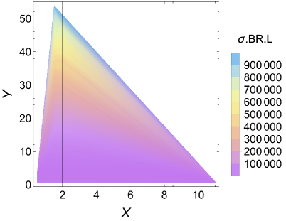
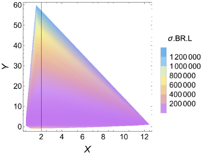
Figure 1: The allowed region in the plane $X$ vs $Y$, using the constraint from the radiative inclusive decay $B\to X_{s}\gamma$. We show the event rates $(\sigma.BR.L)$ at parton level for Scenario Ia (left panel) and Scenario Ib (right panel), where $L$ is the integrated luminosity. We show both scenarios for $L=100$ fb^-1 and taking $m_{H^{\pm}}=110$ GeV.

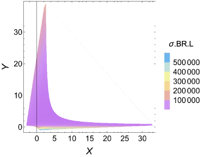
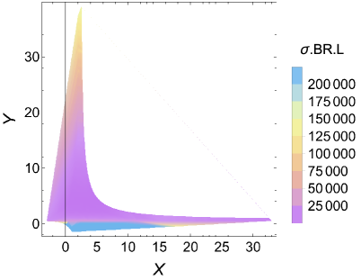
Figure 2: The same as the previous plot for Scenario IIa (left panel) and Scenario Ya (right panel).

5 Backgrounds

There are two groups of SM backgrounds for our signal: the charged-current backgrounds, $\nu t\bar{b}$, $\nu b\bar{b}j$, and photo-production, $e^{-}b\bar{b}j$, $e^{-}t\bar{t}j$. In order to estimate the cross sections of these SM backgrounds, we have used the same preselection as in eq. (5). The expected numbers of events for 100 fb^-1 of integrated luminosity are given in Ref. [6]. Then, we ought to consider, still at parton level (the hadron level analysis is in progress), that the $b$-jets in both signal and background can only be tagged with probability $\epsilon_{b}=0.5$. In the same way, we also adopted mistagging of non-$b$ jets, i.e., treated gluon/light-flavor jets as well as $c$-jets with a probability of $\epsilon_{j}=0.01$ (for $j=u,\,d,\,s,\,g$) and $\epsilon_{c}=0.1$, respectively. With this information, we can apply the tagging probability $\epsilon_{b}^{2}.\epsilon_{c}$ to the signal $S$ and $\epsilon_{b}^{2}.\epsilon_{j}$ to the background $B$. Taking in account these probabilities, we can get the significance at parton level for our benchmark points, which are shown in Tab. 2. With these results one can obtain a significance of 3–4 $\sigma$, with 100 fb^-1 of integrated luminosity for a charged Higgs mass $m_{H^{\pm}}=110$ GeV, $X=Y=5$ in Scenario Ia and Ib. In fact, the same happens for Scenarios IIa and Ya when $X=32$ and $Y=0.5$.

2HDM	$X$	$Y$	$Z$	$m_{H}^{\pm}=110\ {\rm GeV}$
				$cb$	$\sigma.cb$
Ia	5	5	5	0.99	97.36
Ib	5	5	5	0.99	99.80
IIa	32	0.5	32	0.99	92.00
Ya	32	0.5	0.5	0.99	75.12

Table 1: Parameters for a few optimistic benchmark points in the 2HDM-III as a 2HDM-I, -II and -Y configuration. Here cb stands for BR($H^{+}\to c\bar{b}+h.c.$) while $\sigma$.$cb$ stands for the cross section multiplied by the above $BR$ as obtained at the LHeC in units of fb. We have analyzed only the benchmarks where $\sigma.cb$ is greater than 0.15 fb, so that at least 15 events are produced for 100 fb^-1.

(Here, $\epsilon_{b}=0.50,\epsilon_{c}=0.1\ {\rm and}\ \epsilon_{j}=0.01$, where $j=u,d,s,g$) $S$ $B$ $\mathcal{S}=S/B^{1/2}$ Ia ($X=5,Y=5$) $243.4$ $3835.1$ $3.9$ Ib ($X=5,Y=5$) $249.5$ $3835.1$ $4.0$ II ($X=32,Y=0.5$) $230$ $3835.1$ $3.7$ Y ($X=32,Y=0.5$) $187.8$ $3835.1$ $3.0$

Table 2: Significances after 100 fb^-1 for a few optimistic benchmark points in the 2HDM-III as a 2HDM-I, -II and -Y configuration. Here we have considered at parton level the signal reduced by the factor $\epsilon_{b}^{2}.\epsilon_{c}$ while the background from the SM is scaled by $\epsilon_{b}^{2}.\epsilon_{j}$.

6 Conclusions

At the future LHeC, with a integrated luminosity of 100 fb^-1, we found at parton level that a charged Higgs boson of the 2HDM-III would be observed with approximately a 3–4 $\sigma$ significance. At the end of the LHeC era, with $1000$ fb^-1 of data, the detection of such a charged Higgs boson would be certain.

References

- [1] G. Aad et. al. [ATLAS Collaboration], ”Observation of a new particle in the search for the Standard Model Higgs boson with the ATLAS detector at the LHC”, Phys. Lett. B 716, 1 (2012).
- [2] S. Chatchyan et. al. [CMS Colllaboration], ”Observation of a new boson at mass of 125 GeV with the CMS experiment at the LHC”, Phys. Lett. B 716, 30 (2012).
- [3] G. C. Branco, P. M. Ferreira, L. Lavoura, M. N. Rebelo, M. Sher and J. P. Silva, Phys. Rept. 516, 1 (2012) [arXiv:1106.0034 [hep-ph]].
- [4] J. Hernandez-Sanchez, S. Moretti, R. Noriega-Papaqui and A. Rosado, JHEP 1307, 044 (2013)
- [5] J. L. Diaz-Cruz, J. Hernandez–Sanchez, S. Moretti, R. Noriega-Papaqui and A. Rosado, Phys. Rev. D 79, 095025 (2009) [arXiv:0902.4490 [hep-ph]].
- [6] S. P. Das, J. Hernandez-Sanchez, S. Moretti, A. Rosado and R. Xoxocotzi, Phys. Rev. D 94, no. 5, 055003 (2016) [arXiv:1503.01464 [hep-ph]].
- [7] A. G. Akeroyd et al., arXiv:1607.01320 [hep-ph].
- [8] A. G. Akeroyd, S. Moretti and J. Hernandez-Sanchez, Phys. Rev. D 85, 115002 (2012) [arXiv:1203.5769 [hep-ph]].
- [9] H. Fritzsch and Z. z. Xing, Phys. Lett. B 555, 63 (2003) [hep-ph/0212195].
- [10] A. Cordero-Cid et al. ”Impact of a four zero Yukawa texture on and in the framework of the Two Higgs Doublet Model Type III”, JHEP 1407, 057 (2014).
- [11] S. Moretti and K. Odagiri, Phys. Rev. D 57, 5773 (1998) [hep-ph/9709458].
- [12] A. Belyaev, N. D. Christensen and A. Pukhov, “CalcHEP 3.4 for collider physics within and beyond the Standard Model,” Comput. Phys. Commun. 184, 1729 (2013).