A $C^{1}$-continuous finite element formulation for solving the Jeffery-Hamel boundary value problem

Abstract

The third-order Jeffery-Hamel ODE governing the flow of an incompressible fluid in a two-dimensional wedge is briefly derived, and a $C^{1}$ finite element formulation of the equation is developed. This formulation has several advantages, including a natural framework for enforcing the boundary conditions, a numerically efficient solution procedure, and suitability for implementation within well-established, open, scientific computing tools. The finite element formulation is shown to be non-coercive, and therefore not ideal for proving existence, uniqueness, or a priori error estimates, but the numerical solutions computed with quartic Hermite elements are nevertheless found to converge to reference solutions at nearly optimal rates ($\mathcal{O}(h^{4})$ in both $L^{2}$ and $H^{1}$ norms). Further work is required to better understand the cause of the suboptimal convergence rates, and a linear model problem which exhibits analogous characteristics is also discussed as a possible starting point for future theoretical analyses.

1 Introduction

Viscous, incompressible flow in a two-dimensional wedge, frequently referred to as Jeffery-Hamel flow, is described in many references dating back to the original works by Jeffery [1] and Hamel [2], the comprehensive discussion of the various possible configurations of the flow field and a general solution method in terms of elliptic functions by Rosenhead [3], and the modern treatment in fluid mechanics textbooks [4, 5, 6]. Recent research [7] has focused on performing nonlinear stability analyses, computing bifurcation diagrams, and classifying non-unique, stable solutions in various parameter regimes.

In addition to fundamental fluid mechanics research, the Jeffery-Hamel flow solutions are also of great utility as validation tools for finite difference, finite element, and related numerical codes designed to solve the incompressible Navier-Stokes equations under more general conditions. Although a closed-form analytical solution to the Jeffery-Hamel equations is known, it is typically more convenient to work with the solution in a “semi-analytical” form, that is, a form which can be obtained to any desired accuracy using (yet another) numerical method. In this short note, we describe a numerical method based on a $C^{1}$ finite element formulation for efficiently and accurately approximating solutions to the Jeffery-Hamel equations, and compare it to other established techniques in terms of computational expense and implementation difficulty.

The rest of the paper is arranged as follows: the governing equations and the assumptions leading up to them are described in §2. The classical procedure which leads to the semi-analytical form of the solution is described in §3. In §4, the $C^{1}$ finite element method is described. Theoretical aspects related to the existence and uniqueness of solutions to the finite element formulation are discussed in §5. The numerical results are presented in §6, and their accuracy is compared to established methods. Finally, in §7, we summarize the conclusions of this research, and some directions for future work are listed and described.

2 Governing equations

The Jeffery-Hamel solution corresponds to flow constrained to a wedge-shaped region: $r_{1}\leq r\leq r_{2}$, $-\alpha\leq\theta\leq\alpha$. The origin ($r=0$) is a singular point of the flow, and is always excluded from numerical computations. The governing equations are the incompressible Navier-Stokes mass and momentum conservation equations in cylindrical polar coordinates. It is assumed that the flow is purely radial ($u_{\theta}=0$), and the boundary conditions are no slip on the solid walls ($u_{r}(r,\pm\alpha)=0$) and symmetry about the centerline ($\theta=0$) of the channel. Under these assumptions, the incompressible Navier-Stokes equations simplify to:

$$\frac{1}{r}\frac{\partial(ru_{r})}{\partial r} =0$$ (1)

$$u_{r}\frac{\partial u_{r}}{\partial r} =-\frac{1}{\rho}\frac{\partial p}{\partial r}+\nu\left(\frac{\partial^{2}u_{r}}{\partial r^{2}}+\frac{1}{r}\frac{\partial u_{r}}{\partial r}-\frac{u_{r}}{r^{2}}+\frac{1}{r^{2}}\frac{\partial^{2}u_{r}}{\partial\theta^{2}}\right)$$ (2)

$$0 =-\frac{1}{\rho}\frac{\partial p}{\partial\theta}+\frac{2\nu}{r}\frac{\partial u_{r}}{\partial\theta}$$ (3)

where the dynamic viscosity, $\mu$, density $\rho$, and kinematic viscosity $\nu\equiv\frac{\mu}{\rho}$ are given constants which depend on the fluid.

3 Semi-analytical solution strategy

The solution to (1) is particularly simple, and inspires the non-dimensionalization and the form of the eventual solution to the problem. Integrating (1) gives:

$$ru_{r}=F(\theta)$$ (4)

where $F(\theta)$ is a function that depends only on the angular coordinate, $\theta$. Eqn. (4) states that the quantity $ru_{r}$ is constant along any fixed angular direction $\theta=\text{const}$. Since we expect the maximum velocity to occur along the centerline (due to the no-slip boundary conditions on the solid walls), we define the quantity $u_{\text{max}}(r)\equiv u_{r}(r,0)$. This lets us define the constant

$$\lambda\equiv ru_{\text{max}}(r)=\text{const}$$ (5)

That is, the centerline velocity varies with $r$ throughout the domain, but the product $ru_{\text{max}}(r)$ remains fixed. The quantity $\lambda$ has physical units of $\frac{L^{2}}{T}$, and allows us to define the dimensionless Reynolds number for this problem as

$$\text{Re}\equiv\frac{\lambda\alpha}{\nu}$$ (6)

The quantity $\lambda$ can always be computed once Re, $\alpha$, and the fluid property $\nu$ have been specified. Finally, normalizing the angular coordinate according to $\eta\equiv\frac{\theta}{\alpha}$, we obtain the non-dimensional form of (4) as

$$\frac{ru_{r}}{\lambda}=f(\eta)$$ (7)

where $f$ is still an unknown, dimensionless function that depends only on $\eta$, and must satisfy several boundary conditions to be described later. We can rearrange (7) as:

$$u_{r}=\frac{\lambda}{r}f(\eta)$$ (8)

and then, after making the following substitutions

$$\frac{\partial u_{r}}{\partial r} =-\frac{\lambda}{r^{2}}f$$ (9)

$$\frac{\partial^{2}u_{r}}{\partial r^{2}} =\frac{2\lambda}{r^{3}}f$$ (10)

$$\frac{\partial u_{r}}{\partial\theta} =\frac{\lambda}{r}\frac{\partial f}{\partial\eta}\frac{\partial\eta}{\partial\theta}\equiv\frac{\lambda}{r\alpha}f^{\prime}$$ (11)

$$\frac{\partial^{2}u_{r}}{\partial\theta^{2}} =\frac{\lambda}{r\alpha^{2}}f^{\prime\prime}$$ (12)

in (2) and (3), we obtain:

$$-\frac{\lambda^{2}}{r^{3}}f^{2} =-\frac{1}{\rho}\frac{\partial p}{\partial r}+\frac{\nu\lambda}{r^{3}\alpha^{2}}f^{\prime\prime}$$ (13)

$$0 =-\frac{1}{\rho\alpha}\frac{\partial p}{\partial\eta}+\frac{2\nu\lambda}{r^{2}\alpha}f^{\prime}$$ (14)

Multiplying (13) and (14) by $\rho$ and rearranging gives:

$$\frac{\partial p}{\partial r} =\frac{\lambda\mu}{\alpha^{2}r^{3}}\left(f^{\prime\prime}+\alpha\text{Re}f^{2}\right)$$ (15)

$$\frac{\partial p}{\partial\eta} =\frac{2\mu\lambda}{r^{2}}f^{\prime}$$ (16)

The next step is to eliminate $p$ from (15) and (16) in order to solve for $f$. This is accomplished by differentiating (15) with respect to $\eta$, and (16) with respect to $r$, and subtracting. The result is:

$$f^{\prime\prime\prime}+2\text{Re}\,\alpha f\!f^{\prime}+4\alpha^{2}f^{\prime}=0$$ (17)

Equation (17) is a third-order boundary value problem whose description is completed by the specification of the following three boundary conditions:

$$f(0) =1\quad\text{(centerline velocity)}$$ (18)

$$f^{\prime}(0) =0\quad\text{(centerline symmetry)}$$ (19)

$$f(1) =0\quad\text{(no slip)}$$ (20)

Equation (17) has an analytical solution which is given in terms of elliptic integrals, but it is more common (and in many respects simpler) to instead compute a highly-accurate approximate solution to (17) using a numerical method. One possible numerical approach is to rewrite (17) as a system of three first-order ODEs, and use a “shooting method” to iteratively compute solutions until the initial data which produces the desired end condition at $\eta=1$ is obtained. Another possibility is to solve (17) as a boundary value problem using any of a number of numerical procedures which have been developed for this class of problem. The $C^{1}$ finite element solution pursued in the present work falls into this category, and is discussed in further detail in §4.

Once $f$ has been computed numerically, $u_{r}$ follows directly but there is an additional step required to find $p$. Integrating (15) with respect to $r$ yields

$$p=p^{\ast}-\frac{\lambda\mu}{2\alpha^{2}r^{2}}\left(f^{\prime\prime}+\alpha\text{Re}f^{2}\right)+T(\theta)$$ (21)

where $p^{\ast}$ is an arbitrary constant, and $T(\theta)$ is a function of $\theta$ only. Similarly, integrating (16) with respect to $\eta$ gives:

$$p=p^{\ast}+\frac{2\mu\lambda}{r^{2}}f+R(r)$$ (22)

where $R(r)$ is a function of $r$ only. If we make the particular choices

$$T(\theta) \equiv 0$$ (23)

$$R(r) \equiv\frac{2\mu\lambda K}{r^{2}}$$ (24)

where $K$ is a constant, then the pressure fields defined by (21) and (22) are the same if and only if:

$$-\frac{\lambda\mu}{2\alpha^{2}r^{2}}\left(f^{\prime\prime}+\alpha\text{Re}f^{2}\right)=\frac{2\mu\lambda}{r^{2}}(f+K)$$ (25)

or, solving for $K$ in terms of the (now) known function $f$:

$$K=-\frac{1}{4\alpha^{2}}\left(f^{\prime\prime}+\alpha\text{Re}f^{2}\right)-f$$ (26)

Multiplying (26) by $f^{\prime}$ and integrating from 0 to 1 gives:

$$K\int_{0}^{1}f^{\prime}\text{d}\eta=-\frac{1}{4\alpha^{2}}\int_{0}^{1}\left[f^{\prime}\left(f^{\prime\prime}+\alpha\text{Re}f^{2}\right)+4\alpha^{2}ff^{\prime}\right]\text{d}\eta$$ (27)

Applying integration by parts to (27) then results in

$$K\left.f\right|_{0}^{1}=-\frac{1}{4\alpha^{2}}\left[\frac{1}{2}\left.(f^{\prime})^{2}\right|_{0}^{1}+\frac{\alpha\text{Re}}{3}\left.f^{3}\right|_{0}^{1}+2\alpha^{2}\left.f^{2}\right|_{0}^{1}\right]$$ (28)

Finally, substituting in the boundary conditions (18)–(20) gives

$$K=\frac{1}{4\alpha^{2}}\left(\frac{1}{2}f^{\prime}(1)^{2}-\frac{\alpha\text{Re}}{3}-2\alpha^{2}\right)$$ (29)

that is, the value of $K$ depends only on the known constants of the problem and the gradient $f^{\prime}(1)$ at the right-hand boundary. Once $f$, and consequently $K$, are known, the pressure is given (up to an arbitrary constant) by:

$$p=p^{\ast}+\frac{2\mu\lambda}{r^{2}}(f+K)$$ (30)

In a numerical simulation, the arbitrary pressure constant can be selected by “pinning” a single value of the pressure wherever it is convenient, typically on the boundary. Numerically computed $K$ values for some representative (Re, $\alpha$) values are given in Table 1.

Table 1: Values of $K$ for some representative $(\text{Re},\alpha)$ combinations. When the product $\text{Re}\,\alpha>0$, there is an increasingly strong adverse pressure gradient (represented by larger negative $K$ values), and for $\text{Re}\,\alpha>10.31$ the profiles are linearly unstable [3]. When the product $\text{Re}\,\alpha<0$ (hence $\lambda<0$), there is “converging” flow (toward the origin) and the solutions are linearly stable.

$(\text{Re},\alpha)$	$K$
$(30,15^{\circ})$	$-9.7822146449$
$(110,3^{\circ})$	$-1.4387160807\times 10^{2}$
$(-80,5^{\circ})$	$\phantom{-}2.5439853775\times 10^{2}$

4 Finite element formulation

The numerical solution component of the Jeffery-Hamel equations has been tackled by a wide variety of approximation methods over the years. The reasons for the popularity of the equations are quite varied, and include their utility as code verification tools, the ease with which results can be verified against tabulated values in the literature, and the interesting mathematical characteristics—including nonlinearity and higher derivatives—possessed by the equations.

Solution techniques include boundary value problem solvers [8, 9], the modified decomposition method [10, 11], the reproducing kernel Hilbert space method [12], homotopy methods [13, 14, 15], integral transform methods [16], and mixed analytical/numerical solution methods based on computer algebra software [17]. In this work, we pursue a $C^{1}$ finite element solution of (17) in order to show that this variational approach is capable of achieving accurate results in a computationally efficient manner. The prevalence of open source, customizable, and high-quality finite element libraries [18, 19, 20] greatly simplifies the task of implementing such solution algorithms, and helps ensure correct code and the propagation of reproducible, curated results.

The finite element method proceeds by multiplying (17) by a test function $v\in H^{2}(\Omega)$, the Hilbert space of functions with square-integrable second derivatives on $\Omega=(0,1)$, and integrating over the domain to obtain:

$$\int_{0}^{1}\left(f^{\prime\prime\prime}+2\text{Re}\,\alpha f\!f^{\prime}+4\alpha^{2}f^{\prime}\right)v\;\text{d}x=0$$ (31)

Integrating by parts twice on the first term produces:

$$\int_{0}^{1}f^{\prime}\left(v^{\prime\prime}+2\text{Re}\,\alpha fv+4\alpha^{2}v\right)\text{d}x+\left.f^{\prime\prime}v\right|_{0}^{1}-\left.f^{\prime}v^{\prime}\right|_{0}^{1}=0$$ (32)

We then incorporate the boundary conditions (18)–(20) into the test and trial spaces by defining

$$V_{0} =\{v:v\in H^{2}(\Omega),v(0)=v^{\prime}(0)=v(1)=0\}\subset H^{2}(\Omega)$$ (33)

$$S =\{u:u\in H^{2}(\Omega),u(0)=1,u^{\prime}(0)=u(1)=0\}\subset H^{2}(\Omega)$$ (34)

and seek $f\in S$ satisfying:

$$\int_{0}^{1}f^{\prime}\left(v^{\prime\prime}+2\text{Re}\,\alpha fv+4\alpha^{2}v\right)\text{d}x-f^{\prime}(1)v^{\prime}(1)=0\quad\forall\,v\in V_{0}$$ (35)

Introducing a mesh and the finite-dimensional subspaces $V_{0}^{h}\subset V_{0}$, $S^{h}\subset S$ spanned by the basis $\{\phi_{i}\},i=1..N$ leads to the discrete residual statement: find $f_{h}\in S^{h}$ such that $R_{i}(f_{h})=0$ for $i=1..N$, where

$$R_{i}(f_{h})\equiv\int_{0}^{1}f_{h}^{\prime}\left(\phi_{i}^{\prime\prime}+2\text{Re}\,\alpha f_{h}\phi_{i}+4\alpha^{2}\phi_{i}\right)\text{d}x-f_{h}^{\prime}(1)\phi_{i}^{\prime}(1)$$ (36)

The associated Jacobian contribution is given by:

$$J_{ij}(f_{h})\equiv\int_{0}^{1}\left[f_{h}^{\prime}\left(2\text{Re}\,\alpha\phi_{j}\phi_{i}\right)+\phi_{j}^{\prime}\left(\phi_{i}^{\prime\prime}+2\text{Re}\,\alpha f_{h}\phi_{i}+4\alpha^{2}\phi_{i}\right)\right]\text{d}x-\phi_{j}^{\prime}(1)\phi_{i}^{\prime}(1)$$ (37)

The nonlinear system of equations defined by (36) can be solved for $f_{h}$ using e.g. an inexact Newton method which employs high-performance sparse preconditioned Krylov solvers at each iteration.

The simplest and most natural family of finite element shape functions which satisfies the requirements of (36) are the Hermite elements, which are composed of $C^{1}$-continuous polynomials for any order $p\geq 3$. The first four element shape functions (shown in Fig. 1) correspond to the value and gradient degrees of freedom at the left and right nodes, while the higher-order basis functions are “bubbles.” The degrees of freedom associated to the bubble functions could be statically-condensed out of the linear systems before solution, but we do not pursue this optimization in the present work. Finally, we note that the residual (36) and Jacobian (37) contributions require a quadrature rule capable of evaluating polynomials of order $3p-1$ exactly when the underlying basis is of order $p$. For $p=3$, this corresponds to a five point Gauss quadrature rule, while for $p=4$, a six point rule is required.

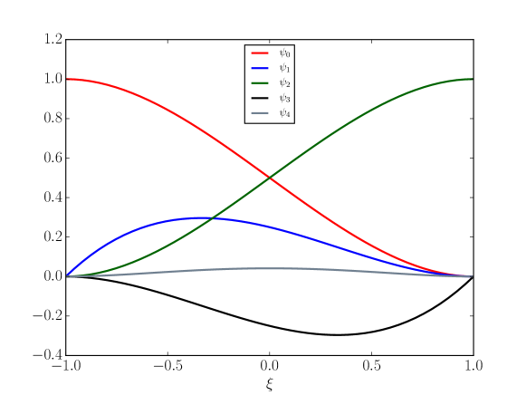
Figure 1: Hermite basis functions up to order $p=4$ in 1D.

5 Existence and uniqueness of solutions

It is reasonable to ask whether a solution to the nonlinear variational problem (35) exists, and if so, whether it is unique. One related theorem is discussed in [21], pg. 472. In abstract notation, the nonlinear problem

$$A(f)=0,\quad f\in X$$ (38)

where $X$ is a reflexive Banach space, has a solution if

1. The operator $A:X\rightarrow X^{\ast}$ is monotone, i.e.

   $$\langle A(f)-A(g),f-g\rangle\geq 0\quad\forall\,f,g\in X$$ (39)

2. $A$ is hemicontinuous, i.e. $A(f+tg)$ converges weakly to $A(f)$ $\forall f,g\in X$ as $t\rightarrow 0^{+}$.

3. $A$ is coercive, i.e.

   $$\lim_{\|f\|_{X}\rightarrow\infty}\frac{\langle A(f),f\rangle}{\|f\|_{X}}=\infty$$ (40)

where the duality pairing is defined in terms of (32) as

$$\langle A(f),v\rangle\equiv\int_{0}^{1}f^{\prime}\left(v^{\prime\prime}+2\text{Re}\,\alpha fv+4\alpha^{2}v\right)\text{d}x+\left.f^{\prime\prime}v\right|_{0}^{1}-\left.f^{\prime}v^{\prime}\right|_{0}^{1}$$ (41)

Unfortunately, it is easy to see that $A(f)$ does not satisfy preconditions 1 and 3 above. For example, to show that $A(f)$ is not coercive, we can directly compute

$$\langle A(f),f\rangle =\int_{0}^{1}f^{\prime}\left(f^{\prime\prime}+2\text{Re}\,\alpha f^{2}+4\alpha^{2}f\right)\text{d}x+\left.f^{\prime\prime}f\right|_{0}^{1}-\left.(f^{\prime})^{2}\right|_{0}^{1}$$

$$=\int_{0}^{1}\left(\frac{1}{2}\left[(f^{\prime})^{2}\right]^{\prime}+\frac{2\text{Re}\,\alpha}{3}(f^{3})^{\prime}+2\alpha^{2}(f^{2})^{\prime}\right)\text{d}x+\left.f^{\prime\prime}f\right|_{0}^{1}-\left.(f^{\prime})^{2}\right|_{0}^{1}$$

$$=-\frac{1}{2}\left.(f^{\prime})^{2}\right|_{0}^{1}+\frac{2\text{Re}\,\alpha}{3}\left.f^{3}\right|_{0}^{1}+2\alpha^{2}\left.f^{2}\right|_{0}^{1}+\left.f^{\prime\prime}f\right|_{0}^{1}$$

$$=-\frac{1}{2}f^{\prime}(1)^{2}-\frac{2\text{Re}\,\alpha}{3}-2\alpha^{2}-f^{\prime\prime}(0)$$ (42)

where the last line follows by imposing the boundary conditions (18)–(20). Thus $\langle A(f),f\rangle$ is not bounded from below by any multiple of $\|f\|_{H^{2}}$, and we conclude that the duality pairing (41) is not coercive.

To show that $A(f)$ is not monotone, let $q\equiv f-g$ for brevity, and directly compute:

$$\langle A(f)-A(g),q\rangle =\int_{0}^{1}\left(q^{\prime}q^{\prime\prime}+2\text{Re}\,\alpha(f-g)(ff^{\prime}-gg^{\prime})+4\alpha^{2}qq^{\prime}\right)\text{d}x+\left.q^{\prime\prime}q\right|_{0}^{1}-\left.(q^{\prime})^{2}\right|_{0}^{1}$$

$$=2\text{Re}\,\alpha\int_{0}^{1}(f-g)(ff^{\prime}-gg^{\prime})\;\text{d}x+\left.q^{\prime\prime}q\right|_{0}^{1}-\frac{1}{2}\left.(q^{\prime})^{2}\right|_{0}^{1}+\left.2\alpha^{2}q^{2}\right|_{0}^{1}$$ (43)

To show lack of monotonicity, we need only find a single $f^{\ast}$ and $g^{\ast}$ for which (39) does not hold. For simplicity, assume that $f^{\ast}=g^{\ast}$ on the boundary, and therefore the boundary terms vanish in (43) vanish, leaving

$$\langle A(f^{\ast})-A(g^{\ast}),f^{\ast}-g^{\ast}\rangle =2\text{Re}\,\alpha\int_{0}^{1}(f^{\ast}-g^{\ast})(f^{\ast}f^{\ast\prime}-g^{\ast}g^{\ast\prime})\;\text{d}x$$ (44)

Next, assume that for this specific choice of $f^{\ast}$ and $g^{\ast}$, the operator is strictly monotone, i.e.

$$\langle A(f^{\ast})-A(g^{\ast}),f^{\ast}-g^{\ast}\rangle>0$$ (45)

Letting $u=-f^{\ast}$ and $v=-g^{\ast}$ in (44) then gives

$$\langle A(u)-A(v),u-v\rangle =-2\text{Re}\,\alpha\int_{0}^{1}(f^{\ast}-g^{\ast})(f^{\ast}f^{\ast\prime}-g^{\ast}g^{\ast\prime})\;\text{d}x$$

$$<0$$ (46)

and therefore the operator $A(f)$ is not monotone.

An existence and uniqueness proof is possible if we instead formulate the problem as a system of nonlinear first-order ODEs by defining: $y_{0}\equiv f$, $y_{1}\equiv f^{\prime}$, and $y_{2}\equiv f^{\prime\prime}$. The third-order ODE (17) can then be written as

$$y_{0}^{\prime} =y_{1}$$ (47)

$$y_{1}^{\prime} =y_{2}$$ (48)

$$y_{2}^{\prime} =-2\text{Re}\,\alpha y_{0}y_{1}-4\alpha^{2}y_{1}$$ (49)

for $\eta\in[0,1]$ (since $f(\eta)$ is symmetric about $\eta=0$) subject to the initial conditions:

$$y_{0}(0) =1$$ (50)

$$y_{1}(0) =0$$ (51)

$$y_{2}(0) =s$$ (52)

where $s$ is unknown, and must be determined iteratively to ensure that the end condition $y_{0}(1)=0$ is satisfied, for example via the shooting method. We can then write equations (47)–(49), (50)–(52) as

$$\vec{y}^{\,\prime} =\vec{F}(\vec{y})$$ (53)

$$\vec{y}(0) =\vec{y}_{0}$$ (54)

By the Picard-Lindelöf theorem [22], if $\vec{F}(\vec{y})$ is Lipschitz continuous in $B_{r}(\vec{y}_{0})$ (a closed ball of radius $r$ centered at $\vec{y}_{0}$), then a unique solution to (53) exists for $t\in[0,\alpha]$, where $\alpha=\min(1,\frac{r}{M})$, and

$$M\equiv\max_{\vec{y}\in B_{r}}\|\vec{F}(\vec{y})\|$$ (55)

In this case, $\vec{F}$ actually has continuously differentiable component functions, which implies Lipschitz continuity, and therefore existence and uniqueness of the solution. Therefore, despite the lack of continuity and monotonicity of the weak formulation of the problem, the ODE formulation suggests there will be a unique solution. Lack of continuity and monotonicity also implies that one cannot prove optimal a priori error estimates for the weak formulation. We will see possible evidence of the effects of non-continuity and non-monotonicity in the convergence results discussed in §6.

6 Results

In this section, convergence results are presented for an implementation of the finite element formulation described in §4 which is based on the libMesh library [23]. Three representative cases are investigated: $(\text{Re},\alpha)=(30,15^{\circ})$, $(110,3^{\circ})$, and $(-80,5^{\circ})$. We also compute a “reference” solution using a custom Python code [24] based on the open source, freely-available scikits.bvp_solver package [8, 9]. This package adaptively controls the amount of error in the numerical solution by increasing the number of subintervals used in the calculation until a user-defined “tolerance” is met. In the present work we set the tolerance to $10^{-14}$, which requires approximately 3200 subintervals in the most expensive case.

We remark that the scikits.bvp_solver implementation is portable, runs in under one second on a reasonably modern laptop, and requires only about 100 lines of Python (including extensive comments). While nearly all authors of new solution techniques for the Jeffery-Hamel equations compare their results to a “reference” solver of some type, they typically do not provide the source code for the reference solver, and/or base it on non-free software such as Matlab, which makes reproducing their results difficult. Therefore, although the code itself is straightforward, we feel that making it readily available is, in itself, an important contribution to the larger field.

Values of $f(\eta)$ at evenly-spaced increments in $\eta$ computed with the $C^{1}$ finite element method described in §4 are given for comparison purposes in Table 2 for the three reference cases. These results, which were computed using a mesh of fourth-order Hermite elements with $h=\frac{1}{320}$, compare favorably with other tabulated values [13, 12] as well as with the reference code used in the present work. The numerical scheme itself performed nearly identically in each of the cases (requiring approximately the same number of nonlinear and linear iterations) and therefore does not appear to be particularly sensitive to the parameters Re and $\alpha$. Since the problem has such modest memory requirements, a direct solver was actually used to precondition the linear subproblems via PETSc’s command line interface.

Table 2: Tabulated values of $f(\eta)$ for several different $(\text{Re},\alpha)$ combinations on a mesh of 320 4th-order Hermite elements.

$\eta$	$(30,15^{\circ})$	$(110,3^{\circ})$	$(-80,5^{\circ})$
0.0	$1.0$	$1.0$	$1.0$
0.1	$9.7312740682\times 10^{-1}$	$9.7923570652\times 10^{-1}$	$9.9596062766\times 10^{-1}$
0.2	$8.9663878283\times 10^{-1}$	$9.1926588558\times 10^{-1}$	$9.8327553811\times 10^{-1}$
0.3	$7.8170458993\times 10^{-1}$	$8.2653361228\times 10^{-1}$	$9.6017991246\times 10^{-1}$
0.4	$6.4348113118\times 10^{-1}$	$7.1022118323\times 10^{-1}$	$9.2352159094\times 10^{-1}$
0.5	$4.9758671435\times 10^{-1}$	$5.8049945880\times 10^{-1}$	$8.6845887923\times 10^{-1}$
0.6	$3.5738880303\times 10^{-1}$	$4.4693506704\times 10^{-1}$	$7.8809092167\times 10^{-1}$
0.7	$2.3268829344\times 10^{-1}$	$3.1740842757\times 10^{-1}$	$6.7314363566\times 10^{-1}$
0.8	$1.2967274302\times 10^{-1}$	$1.9764109452\times 10^{-1}$	$5.1199108961\times 10^{-1}$
0.9	$5.1642634908\times 10^{-2}$	$9.1230421098\times 10^{-2}$	$2.9155874262\times 10^{-1}$
1.0	$0.0$	$0.0$	$0.0$

Convergence results for the cubic and quartic Hermite elements for the three representative cases are given in Fig. 2. Optimal convergence rates for these elements are given by a priori error estimation theory as $p+1$ for $\|e\|_{L^{2}}$ and $p$ for $\|e\|_{H^{1}}$, where $p$ is the polynomial degree. Unfortunately, we observe suboptimal convergence rates in all cases except for the $H^{1}$ error on quartic elements which converges at $\mathcal{O}(h^{4})$. Furthermore, using fifth-order Hermite elements (not shown here) also produces fourth-order accurate results in both $L^{2}$ and $H^{1}$, reductions of 2 and 1 powers of $h$, respectively, from the optimal rates and analogous to the observed reductions for third-order Hermite elements. In summary, we make the following specific observations about the rates of convergence:

• The cubic elements (blue lines in Fig. 2) converge at $\mathcal{O}(h^{2})$ (see Fig. 2(a)) in some cases and $\mathcal{O}(h^{3})$ (see Fig. 2(b)) in others in the $L^{2}$ norm. The rate of convergence therefore seems to depend on the parameters (Re, $\alpha$) which define the problem.

• The cubic elements converge at $\mathcal{O}(h^{2})$ in the $H^{1}$ norm (blue, dashed lines) for all cases.

• The quartic elements converge at $\mathcal{O}(h^{4})$ for both the $L^{2}$ and $H^{1}$ norms for all cases, with the $L^{2}$ norm having a smaller constant.

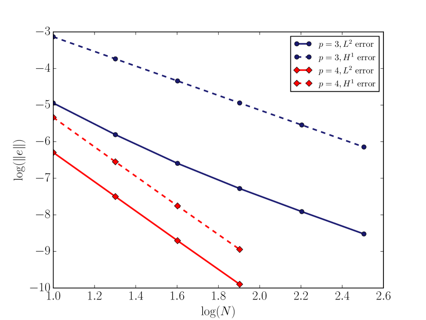
(a) $(30,15^{\circ})$

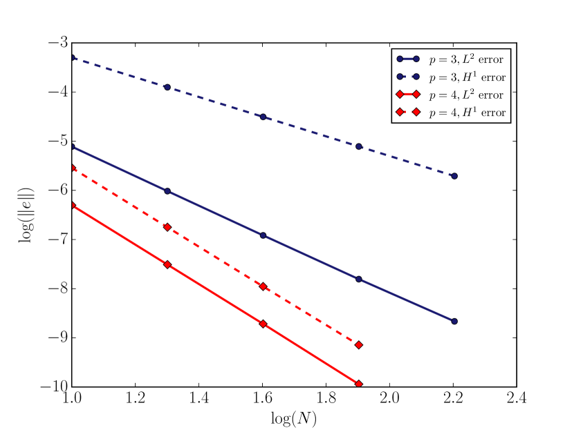
(b) $(110,3^{\circ})$

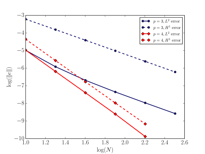
(c) $(-80,5^{\circ})$

Figure 2: Convergence rates for representative cases $(\text{Re},\alpha)=(30,15^{\circ})$, $(110,3^{\circ})$, and $(-80,5^{\circ})$ for cubic and quartic Hermite elements in the $L^{2}$ and $H^{1}$ norms. On the $x$-axis, $N$ is equal to the number of nodes in the finite element mesh, and is therefore proportional to $h^{-1}$.

We currently do not have a complete explanation for the non-optimality in the rates of convergence observed, or the discrepancy between the rates of convergence for the even and odd approximation orders. For linear problems, it is well-known that finite element formulations with non-coercive bilinear forms and mixed formulations that don’t satisfy the inf-sup condition are unstable in the sense that they may produce reasonable results provided that certain conditions are met ($h$ small enough, true solution which does not excite unstable modes, etc.) but they may also produce completely unsatisfactory (numerical oscillations, checkerboard modes, etc.) results. Other than the suboptimal rates of convergence described above, we saw no evidence of unstable modes in the third-order problem discussed here, regardless of (Re, $\alpha$).

In non-coercive problems, stabilizing effects are sometimes achieved by adding bubble functions to the finite element space on each element. Examples include the so-called MINI element [25] for Stokes flow in which cubic bubbles are added to linear triangles in order to satisfy the discrete inf-sup condition, and the addition of cubic bubble functions to stabilize convection-dominated Galerkin discretizations of the convection-diffusion equation [26]. It has also been observed that these bubbles typically have no effect on either the stability or rate of convergence for coercive problems [27].

In the present application, although the formulation is not unstable in the same way that the inf-sup violating and convection-dominated applications are unstable, adding bubbles does have a disproportionate effect on rates of convergence in some cases ($p=3\rightarrow 4$) but not in others ($p=4\rightarrow 5$), and may in some sense be said to have a “stabilizing” effect on the non-coercive formulation. More research, especially on simplified linear model problems, is required in order for this behavior to be fully understood. In §6.1 we briefly discuss additional numerical results for a model problem which exhibits a similar even/odd order convergence rate discrepancy, and might serve as the basis for further theoretical investigations.

6.1 First-order non-coercive problem

To help place the different convergence rates of the even/odd order finite element discretizations of the third-order non-coercive problem into context, we now consider a related problem which is also non-coercive, but is simpler to analyze due to being linear, admits a simpler $C^{0}$ finite element discretization due to having only first-order derivatives, and is trivial to compute the discretization error for. Specifically, we consider the ODE:

$$u^{\prime}+u =g$$ (56)

$$u(0) =1$$ (57)

on $\Omega=(0,1)$, where the forcing function

$$g\equiv\cos\left(\frac{5\pi x}{2}\right)-\frac{5\pi}{2}\sin\left(\frac{5\pi x}{2}\right)$$ (58)

is chosen to produce the exact solution $u=\cos\left(\frac{5\pi x}{2}\right)$, as may be easily verified. The weak formulation proceeds by multiplying (56) by a test function $v\in H^{1}(\Omega)$, integrating over the domain, and integrating by parts on the leading term to obtain:

$$\int_{0}^{1}\left(-uv^{\prime}+uv-gv\right)\text{d}x+\left.uv\right|_{0}^{1}=0$$ (59)

We then incorporate the boundary conditions into the test and trial spaces by defining

$$V_{0} =\{v:v\in H^{1}(\Omega),v(0)=0\}$$ (60)

$$S =\{u:u\in H^{1}(\Omega),u(0)=1\}$$ (61)

and seek $u\in S$ satisfying:

$$\int_{0}^{1}\left(-uv^{\prime}+uv-gv\right)\text{d}x+u(1)v(1)=0\quad\forall\,v\in V_{0}$$ (62)

Introducing a mesh and the finite-dimensional subspaces $V_{0}^{h}\subset V_{0}$, $S^{h}\subset S$ spanned by the basis $\{\phi_{i}\},i=1..N$ leads to the discrete residual statement: find $u_{h}\in S^{h}$ such that $R_{i}(u_{h})=0$ for $i=1..N$, where

$$R_{i}(u_{h})\equiv\int_{0}^{1}\left(-u_{h}\phi_{i}^{\prime}+u_{h}\phi_{i}-g\phi_{i}\right)\text{d}x+u_{h}(1)\phi_{i}(1)$$ (63)

The associated Jacobian contribution is independent of $u_{h}$ for this linear problem, and is given by:

$$J_{ij}\equiv\int_{0}^{1}\left(-\phi_{j}\phi_{i}^{\prime}+\phi_{j}\phi_{i}\right)\text{d}x+\phi_{j}(1)\phi_{i}(1)$$ (64)

We employ the “hierarchic” $C^{0}$ finite element basis functions, which consist of the well-known linear “hat” functions plus bubble functions of increasing order (see Fig. 3), to solve (62) for different polynomial approximation orders $1\leq p\leq 5$. The error between the finite element solution and the known exact solution on a sequence of uniformly-refined grids is plotted in Fig. 4. The results show an odd/even discrepancy in the convergence rates similar to what was seen for the non-coercive third-order problem, however in this case it turns out that the odd-order discretizations are optimal, while it was the even-order discretizations which were pseudo-optimal for the third-order problem.

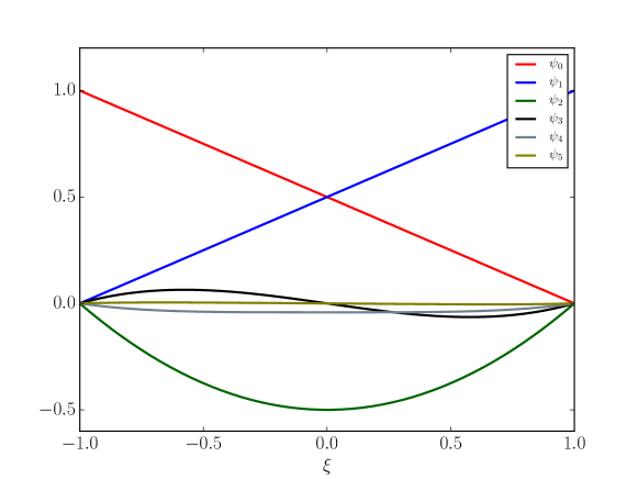
Figure 3: Hierarchic basis functions up to order $p=5$ in 1D.

Finally, we note that pursuing a standard least-squares finite element formulation of (56)–(57) produces a coercive bilinear form, and solutions based on hierarchic finite elements converge to the exact solution at optimal rates in the $L^{2}$ and $H^{1}$ norms regardless of $p$. It therefore seems reasonable that the lack of coercivity is somehow to blame for the suboptimal convergence rates observed in the finite element method, although we do not attempt to develop a theoretical justification of this observation here.

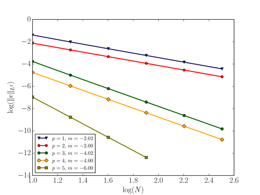
(a) $L^{2}$ error

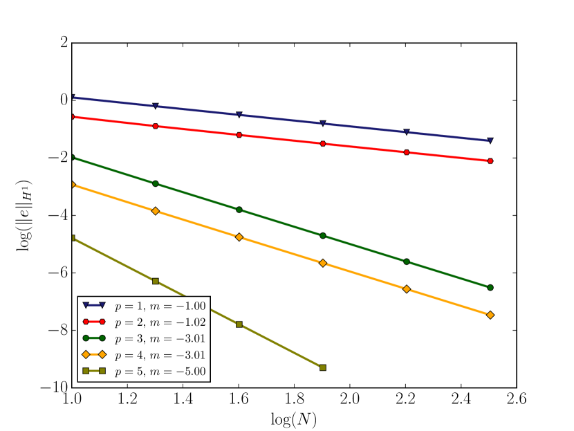
(b) $H^{1}$ error

Figure 4: Convergence rates, $m$, for the non-coercive first-order problem discretized with hierarchic finite elements of order $1\leq p\leq 5$. The odd-order elements exhibit optimal convergence rates while the even-order elements are suboptimal by a factor of $h$ in both the $L^{2}$ and $H^{1}$ norms of the error. Even-order elements of degree $p$ have a slightly better error constant (hence are more accurate) than the corresponding odd-order element of degree $p-1$.

7 Conclusions and future work

Despite the non-optimal rates of convergence observed, the $C^{1}$ finite element formulation for the third-order ODE governing Jeffery-Hamel flow was determined to be a straightforward and numerically efficient solution scheme. Using $C^{1}$ finite elements allows the boundary conditions to be enforced exactly within the finite element basis, and avoids the need to iterate to determine unknown starting conditions as is required in other boundary value problem solution methods such as the shooting method.

The nonlinear systems of equations arising from the finite element formulation are amenable to solution via most common linear algebra packages, and the $C^{1}$ elements themselves are available in several well-established and well-supported finite element libraries, making the method attractive from an implementation standpoint. The finite element solutions have comparable accuracy to a reference boundary value problem solution method in both the $L^{2}$ and $H^{1}$ norms of the error on meshes of $N=160$ elements, regardless of the value of the problem parameters (Re, $\alpha$).

The finite element formulation of the Jeffery-Hamel ODE was shown to be non-coercive, and therefore difficult to demonstrate existence and uniqueness for. Based on ODE existence and uniqueness arguments, however, we do expect such a solution to exist. Additional theoretical investigations, perhaps involving simpler, linear model problems, are warranted to develop a more thorough explanation for the even/odd-order discrepancy observed in the convergence rates for the third-order problem.

A candidate problem demonstrating a similar even/odd order convergence rate discrepancy was described and investigated numerically, but further work is needed to develop both a convergence theory for it, and to apply that theory to the original problem. Finally, since third-order ODEs arise in a number of different semi-analytical and boundary layer solutions of the Navier-Stokes equations, the $C^{1}$ finite element formulation developed here represents another valuable tool in the arsenal of solution methods for such problems, and should be easily extendable to other cases of practical interest.

References

- [1] G. B. Jeffery, “The two-dimensional steady motion of a viscous fluid,” Philosophical Magazine Series 6, vol. 29, no. 172, pp. 455–465, 1915. http://dx.doi.org/10.1080/14786440408635327.
- [2] G. Hamel, “Spiralförmige Bewegungen zäher Flüssigkeiten,” Jahresbericht der Deutschen Mathematiker Vereinigung, vol. 25, pp. 34–60, 1916.
- [3] L. Rosenhead, “The steady two-dimensional radial flow of viscous fluid between two inclined plane walls,” Proceedings of the Royal Society of London A: Mathematical, Physical and Engineering Sciences, vol. 175, no. 963, pp. 436–467, 1940. http://dx.doi.org/10.1098/rspa.1940.0068.
- [4] F. M. White, Viscous Fluid Flow. McGraw-Hill, 2nd ed., 1991.
- [5] R. L. Panton, Incompressible Flow. John Wiley & Sons, 2006.
- [6] W. E. Langlois and M. O. Deville, Slow Viscous Flow. Springer, 2nd ed., 2014.
- [7] P. Haines, R. E. Hewitt, and A. L. Hazel, “The Jeffery-Hamel similarity solution and its relation to flow in a diverging channel,” Journal of Fluid Mechanics, vol. 687, pp. 404–430, Nov. 2011. https://doi.org/10.1017/jfm.2011.362.
- [8] L. F. Shampine, P. H. Muir, and H. Xu, “A User-Friendly Fortran BVP Solver,” Journal of Numerical Analysis, Industrial and Applied Mathematics, vol. 1, no. 2, pp. 201–217, 2006. http://tinyurl.com/jn2zst4.
- [9] J. J. Boisvert, P. H. Muir, and R. J. Spiteri, “A Numerical Study of Global Error and Defect Control Schemes for BVODEs,” Tech. Rep. 2012_001, Department of Mathematics and Computing Science, St. Mary’s University, 2012. http://cs.smu.ca/tech_reports/txt2012_001.pdf.
- [10] M. Kezzar and M. R. Sari, “Application of the generalized decomposition method for solving the nonlinear problem of Jeffery–Hamel flow,” Computational Mathematics and Modeling, vol. 26, pp. 284–297, Apr. 2015. http://dx.doi.org/10.1007/s10598-015-9273-2.
- [11] M. Kezzar, M. R. Sari, R. Adjabi, and A. Haiahem, “A modified decomposition method for solving nonlinear problem of flow in converging-diverging channel,” Journal of Engineering Science and Technology, vol. 10, pp. 1035–1053, Aug. 2015. http://tinyurl.com/pquxb4r.
- [12] M. Inc, A. Akgül, and A. Kiliçman, “A new application of the reproducing kernel Hilbert space method to solve MHD Jeffery-Hamel flows problem in nonparallel walls,” Abstract and Applied Analysis, vol. 2013, p. 239454 (12 pages), 2013. http://dx.doi.org/10.1155/2013/239454.
- [13] S. S. Motsa, P. Sibanda, G. T. Marewo, and S. Shateyi, “A note on Improved Homotopy Analysis Method for solving the Jeffery-Hamel flow,” Mathematical Problems in Engineering, vol. 2010, p. 359297 (11 pages), 2010. http://dx.doi.org/10.1155/2010/359297.
- [14] M. Esmaeilpour and D. D. Ganji, “Solution of the Jeffery–Hamel flow problem by optimal homotopy asymptotic method,” Computers & Mathematics with Applications, vol. 59, pp. 3405–3411, June 2010. http://dx.doi.org/10.1016/j.camwa.2010.03.024.
- [15] A. A. Joneidi, G. Domairry, and M. Babaelahi, “Three analytical methods applied to Jeffery-Hamel flow,” Communications in Nonlinear Science and Numerical Simulation, vol. 15, pp. 3423–3434, Nov. 2010. http://dx.doi.org/10.1016/j.cnsns.2009.12.023.
- [16] Sushila, J. Singh, and Y. S. Shishodia, “A modified analytical technique for Jeffery–Hamel flow using sumudu transform,” Journal of the Association of Arab Universities for Basic and Applied Sciences, vol. 16, pp. 11–15, Oct. 2014. http://dx.doi.org/10.1016/j.jaubas.2013.10.001.
- [17] R. M. Corless and D. Assefa, “Jeffery-Hamel flow with Maple: A case study of integration of elliptic functions in a CAS,” in Proceedings of the 2007 International Symposium on Symbolic and Algebraic Computation (ISSAC’07), pp. 108–115, 2007. http://dx.doi.org/10.1145/1277548.1277564.
- [18] B. S. Kirk, J. W. Peterson, R. H. Stogner, and G. F. Carey, “libMesh: A C++ Library for Parallel Adaptive Mesh Refinement/Coarsening Simulations,” Engineering with Computers, vol. 22, no. 3–4, pp. 237–254, 2006. http://dx.doi.org/10.1007/s00366-006-0049-3.
- [19] W. Bangerth, R. Hartmann, and G. Kanschat, “Deal.II—A general-purpose object-oriented finite element library,” ACM Transactions on Mathematical Software, vol. 33, Aug. 2007. http://doi.acm.org/10.1145/1268776.1268779.
- [20] A. Logg, K.-A. Mardal, and G. Wells, Automated solution of differential equations by the finite element method: The FEniCS book, vol. 84. Springer Science & Business Media, 2012.
- [21] E. Zeidler and L. F. Boron, Nonlinear functional analysis and its applications II/B, Nonlinear monotone operators. New York: Springer-Verlag, 1990.
- [22] E. A. Coddington and N. Levinson, Theory of ordinary differential equations. Tata McGraw-Hill Education, 1955.
- [23] J. W. Peterson, “jeffery_hamel.cc.” GitHub Gist, Dec. 2016. https://gist.github.com/jwpeterson/556be31c41114a41075832c72b3c1616.
- [24] J. W. Peterson, “jeffery_hamel.py.” GitHub Gist, Dec. 2016. https://gist.github.com/jwpeterson/b7381cbd84113bc623185cb552919738.
- [25] D. N. Arnold, F. Brezzi, and M. Fortin, “A stable finite element for the Stokes equations,” CALCOLO, vol. 21, pp. 337–344, Dec. 1984. http://dx.doi.org/10.1007/BF02576171.
- [26] F. Brezzi, M.-O. Bristeau, L. P. Franca, M. Mallet, and G. Rogé, “A relationship between stabilized finite element methods and the Galerkin method with bubble functions,” Computer Methods in Applied Mechanics and Engineering, vol. 96, pp. 117–129, Apr. 1992. http://dx.doi.org/10.1016/0045-7825(92)90102-P.
- [27] L. P. Franca and C. Farhat, “On the limitations of bubble functions,” Computer Methods in Applied Mechanics and Engineering, vol. 117, pp. 225–230, July 1984. http://dx.doi.org/10.1016/0045-7825(94)90085-X.