The Topology of Inter-industry Relations from the Portuguese National Accounts

Abstract

In last years, the Portuguese economy has gone through a severe adjustment process, affecting almost all industrial sectors, the building blocks of economic structures. Research on economic structural changes has made use of input/output tables to define networks of industrial relations. Here, these networks are induced from output tables of the Portuguese national accounting system, being each inter-industry relation defined by the output made by any two industries for the products that they both produce. The topological analysis of these networks allows to uncover a particular structure that comes out during the Portuguese adjustment program. The evolution of the industrial networks shows an important structural change in 2011-2014, confirming the usefulness of inducting similarity networks from output tables and the consequent promising power of the graph formulation for the analysis of inter-industry relations.

Keywords:

Industry/product Output Table, Network Analysis, Minimal Spanning Trees, Industrial Clusters, National Accounting Systems, Proximity Networks

* Corresponding author (tanya@iseg.ulisboa.pt)

Financial support from national funds by FCT (Fundação para a Ciência e a Tecnologia). This article is part of the Strategic Project: UID/ECO/00436/2013.

1 Introduction

As most complex systems, economic structures may be described in many different ways. The simplest descriptions are usually built on top-down decompositions, where aggregation of economic concerns can be either driven by institutional sectors: households, firms and government or by economic outputs as in the three approaches of GDP measurement: the production, expenditure and income approaches.

The economic outputs used in the calculation of GDP by the production approach are collected, validated and reported by national statistical systems. In so doing, these systems organize production by products (goods and services) which are produced by industries. Because each industry is able to produce several goods and since a given good can be the output of various industries, the top-down decomposing chain (sector $\rightarrow$ industry $\rightarrow$ product) may be conveniently replaced by a bottom-up description, where economic structures are built on inter-industry relations. In this setting, it is possible to define each inter-industry relation as the output made by any two industries for the products that they both produce. In so doing, the strength of an inter-industry relation - between any two industries - depends on the number of common products that they share.

The adoption of a bottom-up perspective and the availability of year-based data allows for analyzing the time evolution of inter-industry relations from a network approach. Moreover, such a relational setting provides the basis for evaluating the degree of specialization of the economy from the distribution of its industrial production.

Network approaches are the natural setting for representing and analysing relational linkages. There has been an increasing interest in applying network approaches to economic problems, from the reconstruction of artificial financial markets to the analysis of international trade, there is a great number of successful and inspiring applications ([1]-[9]).The first step in the adoption of a network approach concerns the definition of the network nodes and links. As there are many ways to relate the elementary units of a system, the choices may depend strongly on the questions that a network analysis aims to address [10].

The main objective of this paper is to investigate the extent to which the Portuguese economic performance from 2000 to 2014 had some bearing on the Portuguese inter-industry relations. Given the recent process of strong economic adjustment suffered by the Portuguese economy from 2011 to 2014, we focus on the impact of this process on the Portuguese economic structure which is herein represented by bipartite networks of inter-industry relations.

In many economic networks - and specially in those induced from empirical data - the adoption of a network representation intuitively emerge. It happens because these systems are characterized by a low abstraction level, being the network representation the most obvious solution, as in the case of air-traffic, power-grid, and trade networks.

It also happens with the specific field of input/output (I/O) tables, an important part of the national accounting systems. Because I/O tables are quite similar to adjacency matrices there has been an increased interest in applying network theory to represent money flows between industrial sectors [11]-[17].

In the pioneering work of Slater [12], 75 industries are clustered according to the USA inter-industry flow table of 1967. Later, Schnabl [13] applies Minimal Flow Analysis to induce networks from the German I/O tables reporting data in between 1978 and 1988. There, centrality measures allow for classifying industries into three different sectors (source, sink and center). More recently, Blöchl and co-authors [11], using I/O tables of 37 OECD countries, induce networks of industries to which measures of random walk centrality and counting betweenness are applied. Their results have shown the suitability of those measures in the identification of groups of countries according to their development status.

The present study also falls into the broad category of data-driven investigation on industrial relations using a network approach. Nevertheless, we follow a different perspective. Instead of considering I/O tables, we take the output of each industry distributed by the set of products that this industry produces. Inter-industry relations are then defined by the production of common products. Industries are linked whenever they share at least one mutual product, being the strength of each inter-industry link defined by the output made by the involved industries for the products that they both produce. In so doing, the intensity of a link between any two industries depends on the number of mutual products weighted by their relative (output) values in each linked industry.

The networks we work with are proximity (and bipartite) networks. In proximity networks, the links are defined from shared features, correlation coefficients or other well-defined similarity measures. Like in many other economic networks, the elementary units do not have to be explicitly linked by any concrete relation existing in the real world except for a well-defined measure of distance in between them. Although the induction of proximity networks is less intuitive than those obtained from the air-traffic, power-grid or I/O table examples, they provide useful analytical settings, being found in a multitude of applications. Examples of proximity networks in Economics can be found in references [18] ,[19] and [20]. A detailed discussion on proximity networks is presented in reference [10].

The paper is organized as follows. Section two presents the data we work with. Section three is targeted at presenting the methodological aspects and a brief discussion on the first results. Section four discuss the evolution of the Portuguese industrial networks, focussing on the topological analysis of different time periods . Finally, Section five presents the concluding remarks.

2 The data

Our data source is the year-based Industry/Product output tables ($OT^{t}$ $t=2000,2001,...,2014$) compiled by the Portuguese national accounting agency (INE [21]). The output tables consist of data on production values (at market prices) organized by industry and related products. In this context, industries (I) refer to firms and other business, and the products (P) refer to goods and services. Moreover, while the classification of a given business into a specific industrial category (I) is determined by its economic activity classification (NACE code) by taking into account the main activity of the firm; products (P) are classified by activity according to a statistical coding (CPA code).

There are international standards for the industry (and product) classification sets provided by the United Nations (UN) and adopted by most of countries. The UN System of National Accounts (SNA) provides the basis for uniformity among the various data sets, while the OECD industry classifying into 10, 21 and 38 industries makes the international comparisons possible [22].

Table 1 shows a snapshot of the classifying list of industries and products according to NACE and CPA codes at the resolution of 38 industries and 38 products (I38 & P38). Table A (in the appendix) provides a complete presentation of the industries and products at the same resolution.

Because the classification of each industry is determined by its main economic activity, which in turn is determined by the type of goods or services it produces, the classification of industries happens to be identical to the classification of products, as the last two columns of Table 1 show. Moreover, except for the public administration industry (O), the production of every industry relies mainly on a specific product whose code is naturally inherited from the industry itself. Even though, industries do produce several other products, besides the main (self-coded) products, each of which happens to be the output of various industries.

NACE and	Description	I38	P38
CPA code
01-03	Agriculture, forestry and fishing	A	A
05-09	Mining and quarrying	B	B
10-12	Food products, beverages and tobacco products	CA	CA
13-15	Textiles, wearing apparel, leather and related products	CB	CB
16-18	Wood and paper products, and printing	CC	CC
…	…	…	…
41-43	Construction	F	F
45-47	Wholesale and retail trade	G	G
…	…	…	…
64-66	Financial and Insurance	K	K
68	Real estate	L	L
…	…	…	…
97	Households as employers of domestic personnel	T	T
99	Activities of extraterritorial organizations and bodies	U	U

Table 1: A snapshot of the list of industries and products according to NACE and CPA codes at the resolution I38 & P38.

Our approach is applied to a data set comprising 15 output tables ($OT_{38}^{t}$ $t=2000,2001,...,2014$) at the resolution of 38 industries and 38 products (I38 & P38) reported by INE. Table 2 shows part of the Industry/Product output table of 2000 ($OT_{38}^{2000}$), a framework where each industry is associated with the set of products it produces. Each cell in $OT_{38}^{2000}$ represents the value $v^{{}^{2000}}(i,p)$ of the output $p$ produced by industry $i$ in 2000.

	I38/P38	P1	P2	…	P36	P37	P38
		A	B	…	S	T	U
I1	A	6375238	96	…			-
I2	B	0	837319	…			-
…	…	…	…	…	…	0	-
I36	S	0	0	…	1513029	0	-
I37	T	0	0	0	0	494448	-
I38	U	-	-	-	-	-	-

Table 2: Part of the industry/product output table at the resolution I38 & P38 (values in 10³ euros).

Since our main focus relies on the analysis of the most recent years, Table 3 shows the number of products ($\#p$) by industry in 2010 and 2014. Because some products are not produced at a significant level, we added columns (#$p$>10⁶) with the number of products whose output values are above one million euros. When considering the significant levels of production, the vast majority of industries produced between 6 and 15 products. In opposing situations are the industries G (Wholesale trade) and T (Goods and services producing activities of households for own use) presented at the last row of Table 3. The former produces just one product while the latter, produces more than 30 products, both in 2010 and 2014.

Industry	2010		2014		Industry	2010		2014
	$\#p$	#$p$>106	$\#p$	#$p$>106		$\#p$	#$p$>106	$\#p$	#$p$>106
A	16	10	15	10	H	15	14	15	12
B	11	7	10	7	I	12	10	13	9
CA	12	9	12	7	JA	16	10	15	8
CB	20	14	17	12	JB	12	10	12	10
CC	19	16	19	13	JC	11	7	12	7
CD	7	6	6	6	K	7	7	6	6
CE	16	13	15	12	L	10	8	8	6
CF	11	6	10	6	MA	14	10	12	9
CG	20	15	20	16	MB	14	5	15	7
CH	20	14	20	14	MC	13	6	12	8
CI	16	12	15	12	N	10	6	10	6
CJ	17	12	16	13	O	28	20	27	21
CK	17	12	16	12	P	24	13	21	13
CL	17	14	16	13	QA	19	11	17	12
CM	20	18	20	17	QB	24	9	19	9
D	10	6	10	6	R	18	10	17	10
E	16	11	15	11	S	11	7	11	7
F	15	15	18	15	T	1	1	1	1
G	32	32	32	32	U	0	0	0	0

Table 3: Number of products by industry and number of products produced at a significant level, at the resolution I38 & P38.

Figure 1 shows the distribution of the number of products by industry in 2010 and 2014, together with the information provided in Table 3, those distributions suggest that:

1. there is a slight increase in diversification of production from 2010 to 2014

2. the number of products produced by industries G (Wholesale trade) and CC, CG, CF, CH and CM (manufacturing industries) remains almost unchanged (Figure 1(a))

3. the number of products produced by industries F (Construction) increases significantly from 2010 to 2014 but the number of those produced at a significant level remain unchanged

4. the strongest difference between the number of products and those produced at a significant level relies on the industries O (Public administration), P (Education), QA (Human health) and QB (Social work)

5. the highest decreases from 2010 to 2014 in the number of products produced at a significant level (Figure 1(b)) occurs in industries CB (Textiles) and L (Real state)

6. among the few industries that display an increase in the number of products produced at a significant level are MB (R&D) and MC (Other professional, scientific and technical services)

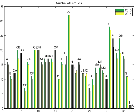
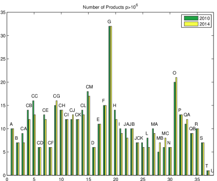
Figure 1: a: The number of products by industry at the resolution of 38 industries and 38 products in 2010 and 2014 and b: The number of products produced at a significant level, at the resolution of 38 industries and 38 products in 2010 and 2014.

3 Networks

As earlier mentioned, in defining any network, there are many different design decisions to be taken. The choice of a given set of nodes and the definition of the links between them is only one out of several other ways to look at a given system. Here we define year-based bipartite networks where similarities between industries are used to set the existence of every link in each network. Being weighted graphs, the weight of each link is proportional to the intensity of the similarity between the linked pair of industries, relative to the overall output value of each involved industry.

Because those bipartite networks have a large number of links, we compute their corresponding Minimal Spanning Trees (MST). In fact, it happens that when networks are induced from similarity measures, the issue of deriving a sparse network from a dense or even a complete one becomes meaningful. The less arbitrary choices (or the most endogenously based ones) usually relies on the construction of a MST. In so doing, we ensure the connectivity is preserved (the resulting network is necessarily connected) while moving from a dense network to a sparse one. Moreover, we are able to emphasize the main topological patterns that emerge from the network representations. Beyond the MST analysis, we evaluate and discuss the amount of redundancy in the network links and the values of the residuality coefficient computed for each year-based network of industries. These coefficients - redundancy and residuality - help to characterize the main differences in the behavior of those networks in the latest years.

3.1 Bipartite Graphs

A bipartite network $N$ consists of two partitions of nodes $I$ and $P$, such that edges connect nodes from different partitions, but never those in the same partition. A projection of such a bipartite network onto $I$ is a network consisting of the nodes in $I$ such that two nodes $i$ and $i\prime$ are connected, if and only if there exist a node $p\in P$ such that $(i,p)$ and $(i\prime,p)$ are edges in the corresponding bipartite network ($N$).

Here, the two partitions of nodes $I$ and $P$ are the set of industries and the set of products, respectively, both at the resolution of 36 elements, as presented in Table A1 (and partially displayed in Table 2). The links between any two industries $(i,i\prime)$ in  the network $N$ are defined by the existence of products ($p\in P$) such that $(i,p)\in$ $N$ and $(i\prime,p)\in$ $N.$

In the following, we explore bipartite networks and their corresponding projections $N_{36}^{t}(i,p)$ where $t=2000,2001,...,2014$ with $i$ $\in$ {I₁,I₂ ,…, I₃₆} and $p\in$ {P₁,P₂ ,…, P₃₆}.

3.2 Networks of Industries

Given that each industry can produce many products and that each product can be produced by several industries, from each output table, the values $v^{t}(i,p)$ $t=\{2000,2001,...,2014\}$ with $i$ $\in$ {I₁,I₂ ,…, I₃₆} and $p\in$ {P₁,P₂ ,…, P₃₆} relating industries to products are taken and the proximity networks $N_{36}^{t}$ are induced. There, nodes are industries (I_i $i$ $\in$ {I₁,I₂ ,…, I₃₆} and links $n_{(a,b)}$ are defined by:

$$n_{(a,b)}=\sum_{k=1}^{36}p_{ak}p_{bk}$$ (1)

where the $p_{ik}$ and $p_{jk}$ are the normalized values of the outputs of industries $i$ and $j$ for the product $k$, respectively.

The values $v(a,k)$ of the product $k$ produced by industry $a$ are normalized by industry, summing up the output values of all the products ($k)$ that industry $a$ produces:

$$p_{ak}=\frac{v(a,k)}{\sum\limits_{k=1}^{k=36}v(a,k)}10^{3}$$ (2)

Therefore, the higher is the value of the mutual production of two industries (nodes $I_{a}$ and $I_{b}$), the greater is the strength of the connection ($n_{(a,b)}$) between industries $a$ and $b$.

As an example, and taking from the output table $OT_{38}^{2014}$ the normalized values (Eq.2) of each mutual product produced by industries QA (Human health) and QB (Social work) in 2014 yields (Eq.1) $n_{QA,QB}=0.84$ while, for instance, $n_{CI,CJ}=94.65$, since the normalized values (Eq.2) of each mutual product produced by industries CI (Manufacture of computer, electronic and optical products) and CJ (Manufacture of electrical equipment) in 2014 gives (Eq.1) $94.65$ . Not surprisingly, the link between industries CI (Manufacture of computer, electronic and optical products) and CJ (Manufacture of electrical equipment) is around 100 times stronger than the connection between industries QA (Human health activities) and QB (Social work activities), as the second graph in Figure 2 shows.

A multitude of different connection strengths can be observed in the networks N${}_{36}^{2000}$ and N${}_{36}^{2014}$ presented in Figure 2. They are weighted networks where the width of the links is proportional to the strength of the connection between the involved nodes, and the size of the nodes is proportional to their Gross Value Added (GVA).

The first graph in Figure 2 (Figure 2(a)) shows that industries G (Wholesale trade), O (Public administration), F (Construction) and L (Real state) are those with the highest GVA (the largest nodes) in the entire graph. The network at the right side of Figure 2 (Figure 2(b)) shows that industries MB (R&D)  and N (Education) display increased sizes (larger GVA) when compared with their situation in 2000. Moreover, the industries F (Construction) and K (Financial services) are among those with the highest decrease of GVA in 2014. It happens together with the significant decrease in the number of products of industry F in 2014 when compared with 2000. Figure 2 also shows that the link between industries CI (Manufacture of computer, electronic and optical products) and CJ (Manufacture of electrical equipment) is largely reinforced in 2014, while the connection between CF (Pharmaceuticals) and G (Wholesale trade) loses weight when compared with 2000.

The overloaded graphs presented in Figure 2 do not favor the observation of any particular pattern besides those associated with the size of the nodes and links in each of those years.

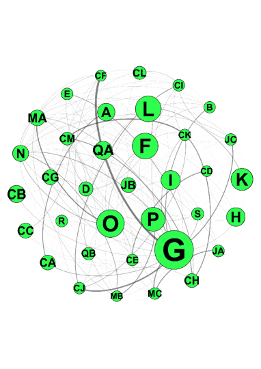
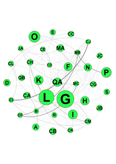
Figure 2: The networks of industries $N_{36}^{2000}$ and $N_{36}^{2014}$.

Undoubtedly, the networks above presented are not very informative about any emerging structure in the network of industries. As earlier mentioned, when networks are induced from similarity measures, in deriving a sparse network from a dense one, the less arbitrary choices (or the most endogenously based ones) usually rely on filtering the complete network with the threshold distance value used in the last step of the hierarchical clustering process of the construction of a Minimum Spanning Tree (MST). In so doing, we ensure the connectivity is preserved since the resulting network is necessarily connected.

3.3 Minimum Spanning Trees

A MST of a connected and weighted graph can be constructed by taking its nodes and links and applying the nearest neighbor method. The first step in this direction is the computation of the distances $d_{ij}$ between each pair of nodes $i$ and $j$ as the inverse of the weight of the link between them:

$$d_{ij}=\frac{1}{n_{ij}}$$ (3)

From the distance matrix $D_{36}^{t}$ a hierarchical clustering is then performed. Initially $36$ clusters corresponding to the 36 industries are considered. Then, at each step, two clusters $c_{i}$ and $c_{j}$ are clumped into a single cluster if

$d\{c_{i},c_{j}\}=\min\{d\{c_{i},c_{j}\}\}$

with the distance between clusters being defined by

$d\{c_{i},c_{j}\}=\min\{d_{pq}\}$ with $p\in c_{i}$ and $q\in c_{j}$

This process is continued until there is a single cluster. In a connected graph with $n$ nodes, the MST is a tree of $n-1$ edges that minimizes the sum of the edge distances. In a network with $36$ nodes, the hierarchical clustering process takes $35$ steps to be completed, and uses, at each step, a particular distance $d_{i,j}$ $\in$ $D_{36}^{t}$ to clump two clusters into a single one.

Let $C=\{d_{q}\}$, $q=1,...,m$, be the set of distances $d_{ij}\in D_{36}^{t}$ used at each step of the clustering and the threshold distance $L_{36}^{t}=\max\{d_{q}\}$. After the last step, we are able to define a representation of $D_{36}^{t}$ with sparseness replacing high-connectivity in a suitable way. In the next section, we analyze the evolution of the threshold distance $L_{36}^{t}$ $\ t=2000,2001,...,2014$ with particular attention to the behavior of $L_{36}^{t}$ after 2010.

4 Results

Figure 3 shows the MST of the networks N${}_{36}^{2000}$, N${}_{36}^{2005}$ where the size of the nodes remain defined as in Figure 2, being proportional to the yearly amount of GVA of each industry. Here, nodes are colored according to their partition clusters, computed by a community detection algorithm [23] available at Gephi, an open source software for exploring and manipulating networks (https://gephi.org).

Four partition clusters are defined, they are:

1. Trade (green): is the larger cluster, comprising industries A (Agriculture and fishing), CA (Food products and beverages), and CB (Textiles).

2. Construction (red): is the most adversely affected cluster after 2005. Besides industry F (Construction), it comprises L (Real estate) and K (Financial services).

3. Manufacture (blue): is the most stable cluster, comprising CH (Basic metals), CK (Machinery) and CM (Furniture).

4. Arts (yellow): is the less stable cluster. It is made of  industries R (Arts), JA (Publishing) and MC (Scientific and technical services).

In the networks presented in Figures 3 and 4, white nodes represent those whose inclusion into a specific cluster is largely unstable over the 15 years period 2000-2014. They are made by industries CG (Rubber and plastics), CE (Manufacture of chemical services) and CD (Petroleum, mineral and chemical products). After 2010, industries A (Agriculture and fishing) and CA (Food products and beverages) join this weakly related group of industries while industry CG (Rubber and plastics) leaves it.

Table 4 shows the four partition clusters and the main nodes in each cluster. Despite of the structural evolution of the networks over the 15 years, these are the nodes whose clustering membership remains unchanged.

Cluster		Color	Main Nodes
1	Trade	green	G	A	CA
2	Construction	red	F	L	K
3	Manufacture	blue	CH	CK	CM
4	Arts	yellow	R	JA

Table 4: Industrial Clusters.

The order these clusters are ranked in Table 4 is in line with the results presented in reference [11] where two measures of node centrality are defined and applied to data from I/O tables of 37 countries, Portugal included. The authors showed that, near the year of 2000, Trade is most frequently the sector with the highest random walk centrality, being replaced by the Construction cluster in countries like France and Ireland.

The trees in Figure 3 show that the inter-industry relations suffer a small change from 2000 to 2005.

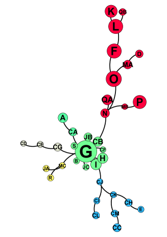
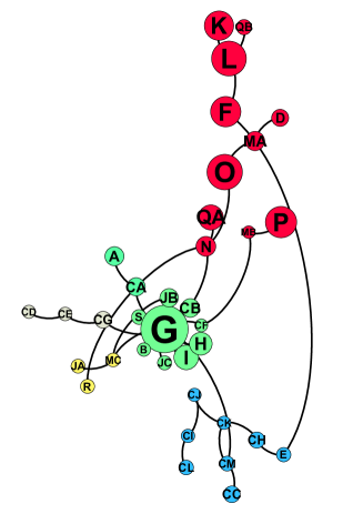
Figure 3: The MST of the networks $N_{36}^{2000}$ and $N_{36}^{2005}$.

Being each of them a MST with 36 nodes, they have exactly 35 links. Let us define $RL_{2000}^{2005}$ $\in\{0,1,2,...35\}$ as the number of replaced

links from $MST^{2000}$ to $MST^{2005}$. It happens that $RL_{2000}^{2005}$ $=5$, due to the few changes occurring from 2000 to 2005, they are: i) industries I (Accommodation) and H (Transportation) lose their links to Construction and Manufacture clusters, respectively, turning both to be connected to Trade; ii) in the opposite direction, industries CI (Electronics) and CJ (Electrical equipment) lose their links to Trade and turn to be connected to the Manufacture cluster. At last, there is a new link between industries O (Public administration) and N (Administrative services).

In line with the small value of $RL_{2000}^{2005}$, the links inside each cluster remain almost unchanged from 2000 to 2005. Even the small groups of white nodes, as the one formed by industries MC (Other professional, scientific and technical services), JA (Publishing activities) and R (Arts) and those comprising the core of the Manufacture cluster (CD, CE and CG) remain without modifications over that five years period.

Figure 4 shows $MST^{2010}$ and $MST^{2014}$. Looking at the differences between the networks in the last graph of Figure 3 and the first graph in Figure 4, we see that from 2000 to 2010, the industries in the Construction (red) cluster are the most adversely affected being those with the larger reduction in the number of inter-industry relations. We envision that is comes from an increase in diversification since these industries reduced their production values but maintained (or even enlarged) the diversity of their products.

When the observation of these networks is complemented with the information on the distribution of the number of products by industry (presented in Figure 1)  it turns out that the Construction industry seems to be the most affected one. As earlier mentioned, it is a consequence of the decline in the construction of buildings followed by a corresponding decrease in Real estate (Leasing and transactions of buildings). In that same period, G (Wholesale trade) maintains its production level and reduces the output of the less relevant products.

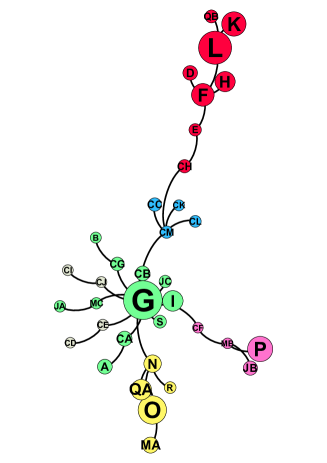
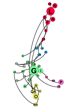
Figure 4: The MST of the networks $N_{36}^{2010}$ and 2014 $N_{36}^{2014}$

Conversely to what happened in the comparison of 2000 and 2005, the trees in Figure 4 show that the inter-industry relations suffer a large change from 2010 to 2014. The number of replaced links reaches 17 ($RL_{2010}^{2014}=17$), showing that almost half of the connections is replaced. Such a large structural modification affects all clusters and brings an entirely new shape to $MST^{2014}$. The main changes concern: i) the breakdown of the Manufacture (blue) cluster, where almost every link existing in 2010 is removed; ii) a great reduction of the number of links inside the Trade cluster, iii) the loss of linkage between the industries MC (Other professional, scientific and technical services) and JA (Publishing), iv) industry CI (Computer industry) turns to be linked to the former Manufacture cluster while losing its links to Trade. Moreover, v) the Construction cluster that shrunk even before 2010 does not recover in 2014 vi) the emergence of a link between the industries MC (Other professional, scientific and technical services) and R (Arts) reinforces the connection between industries in the service sector. Finally, vii) in 2014 the link between the industries MB (R&D) and JB (Telecom) disappears, which can be associated to a decrease in investment in innovation made by telecom companies. On the other hand, the link between the industries MB (R&D) and the CF (Pharmaceutical) remains, in line with the increasing high level of R&D participation in the pharmaceuticals since 2010, when these industries form a new cluster (pink), as the graphs in Figure 4 show.

To better evaluate the structural changes that characterize the inter-industry relations, the plots in Figure 5 show the evolution of the threshold distance ($L^{t}$) in $N_{36}^{t}$ $t=2001,2002,..,2014$ and the evolution of the number of replaced links $RL_{t-1}^{t}$ over the same period.

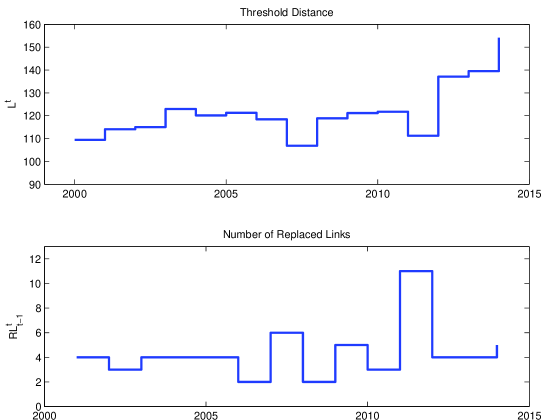
Figure 5: The Threshold Distance $L^{t}$ and the number of Replaced links $RL_{t-1}^{t}$ in each $MST_{36}^{t}$.

The evolution of $L^{t}$ along the 15 years period shows an important increase of the threshold distance in 2012 after a decrease in 2011. After 2012 the threshold distance value tends to remain almost unchanged and the corresponding network structures display a small number of replaced links, as the last years in the plots of Figure 5 show. Increases in the threshold distance mean that at least one of the network links becomes weaker, leading to the consideration of a set of larger distances in the hierarchical clustering process that defines the MST.

Meanwhile, there is a remarkable increase in the number of replaced links from 2011 to 2012. Earlier we saw that the number of replaced links from 2010 to 2014 ($RL_{2010}^{2014}=17$) reaches 17, showing that almost half of the connections is replaced in between those four years. Looking to the evolution of $RL_{t-1}^{t}$ on a yearly-basis suggests that most of the replacements occurs from 2011 to 2012, over the first year of the Portuguese economic adjustment.

In fact, it is worthy of attention that those important structural changes are concentrated in the Portuguese economic adjustment period, providing therefore enough evidence of the contribute that such network approach brings to answering our main research question.

4.1 Beyond the trees

In the last section, we saw that the large number of links in each network $N_{36}^{t}$ makes the extraction of their truly relevant connections a challenging problem. There, the construction of each MST allowed for the definition of networks where sparseness replaces high-connectivity in a suitable way.

However this construction neglects part of the information contained in the distance matrix, since it only takes the $35$ distances that are considered in the hierarchical clustering process.

In order to avoid this loss of information we define the projected graph $B_{36}^{t}$ (with $N_{36}^{t}$ vertices being the network nodes) by setting $b_{i,j}$ $=d_{i,j}$ if $d_{i,j}<$ $L_{36}$ and $b_{i,j}=0$ if $d_{i,j}$ $>L_{36}^{t}$. As usual, null arcs of $B_{36}^{t}$ are those for which $b_{i,j}=0$. Here we want to consider two nodes $i$ and $j$ to be connected if $d_{i,j}<$ $L_{36}$.

Let $A_{36}^{t}$ be the boolean graph associated with $B_{36}^{t}$, where each element $a_{i,j}$ is the number of edges of $B_{36}^{t}$ that join the vertices $i$ and $j$ and, since $B_{36}^{t}$ is a simple graph, $a$ $\in$$\{0,1\}.$

Let us also define $C^{\ast}=\{d_{l}\}$, $l=1,...,m$, as the set of distances $d_{ij}\in D_{36}^{t}$ whose values are less or equal to $L_{36}^{t}$ and compute $S^{t}$

$$S^{t}=m-35$$ (4)

as the number of redundant elements in $C^{\ast}$, that is, the number of distances $d_{ij}$ that, although being smaller than $L_{36}^{t}$,  are not considered in the hierarchical clustering process [24]. The first plot in Figure 7 shows the evolution of $S^{t}$. Besides the behavior of $S^{t}$, a detailed way to look at modifications in the number of redundant elements of the networks can be observed in the following graphs.

The four plots in Figure 6 show the boolean graphs ($A_{36}^{t}$) obtained for the years 2000, 2005, 2010 and 2014. They were obtained by:

1. Taking the matrix of distances ($D_{36}^{t}$) of each period ($t=2000,2005,2010,2014$).

2. Applying the hierarchical clustering process to obtain the threshold distance $L_{36}^{t}$ used in the last step of the hierarchical clustering process.

3. Building the corresponding boolean graph ($A_{36}^{t}$) where unit arcs ($d_{ij}^{t}\leq L_{36}^{t}$) are represented as black patches and null arcs ($d_{ij}^{t}>L_{36}^{t}$) correspond to white ones.

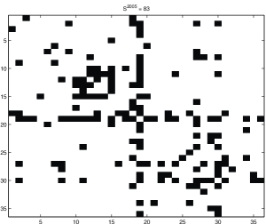
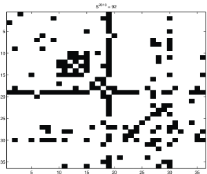
Figure 6: The boolean graphs (a) 2000 (b) 2005 (c) 2010 and (d) 2014.

The boolean graphs in Figure 6 show the structure of inter-industry relations in each of the chosen years. There is a relevant difference in 2014, as the graph in Figure 6(d) shows. The number of black patches strongly increases in the structure represented in the last graph of Figure 6, showing that the number of unit arcs is much greater than 35. Consequently, the number of redundant elements in the graph is significantly greater than in the other three graphs. As shown in this figure, the network structure in 2014 tend to contain cycles and moves away from the tree-like structures that characterize those obtained for 2000, 2005 and 2010 (graphs (a), (b) and (c) in Figure 6).

As we aim at characterizing the richer connectivity structure that emerges in 2014, besides the topological coefficient $S^{t}$ that captures the number of redundant elements in the networks, we compute the residuality coefficient $R^{t}$ [24], targeted at measuring the amount of residuality in each network $N_{36}^{t}$.

$$R^{t}=\frac{\sum_{d_{i,j}>L}d_{i,j}^{-1}}{\sum_{d_{i,j}\leq L}d_{i,j}^{-1}}$$ (5)

where $L_{36}^{t}$ is the threshold distance value that insures connectivity of the whole network in the hierarchical clustering process.

The evolution of $S^{t}$ along the 15 years period is presented in the first plot of Figure 7. The value of $S^{2014}$=138 shows an important increase in the number of redundant links. Our previous studies ([18],[19],[24],[25]) revealed that the observation of an important increase in redundancy use to be a consequence of disturbed periods being the topological correlate of the occurrence of stress events. Here, the large increase in the number of redundant elements from 2012 to 2014 provides enough evidence of the structural changes taking place on the network structure after the implementation of the economic adjustment program in Portugal.

The coefficient of residuality relates the relative strengths of the links above and below the threshold distance value ($L_{36}^{t}$). In other words, it relates the relative strengths of weak and strong links. Increases in $R_{36}^{t}$ usually happen because strong ties become even stronger (short distances are shortened). Moreover, it also comes from the fact that the networks become less sparse (the number of links increases), forcing several weak links to leave this category. These structural reinforcement is often associated with the occurrence of stress events, as the implementation of the recent process of Portuguese economic adjustment.

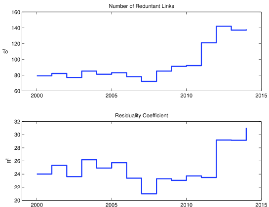
Figure 7: The number of Redundant links $S^{t}$ in the networks $N_{36}^{t}$ and the Residuality Coefficient $R^{t}$.

The plots in Figure 7 show the evolution of the residuality coefficient ($R^{t}$) in the networks $N_{36}^{t}$ $t=2000,2001,..,2014$ and the evolution of the ($S^{t}$) in the same time interval. They allow for capturing the main differences in the behavior of these coefficients in the latest years. Indeed, the plots in Figure 7 show that the lowest values of $S^{t}$ and $R^{t}$ correspond to the years before 2011. After 2011, as revealed by the strong increase of $S^{t}$ and $R^{t},$ a major change is occurring in the structure of the networks $N_{36}^{2012},N_{36}^{2013}$ and $N_{36}^{2014}$. This change, being empirically described, suggests that in the recent process of economic adjustment suffered by the Portuguese economy, a new structure emerges from the inter-industry relations.

5 Conclusion

The literature has shown an increasing use of Input/Output tables to induce networks of money flows between industries in national economies. Because I/O tables are quite similar to adjacency matrices, their representation as networks intuitively emerges. Here we follow a similar approach but instead of the usual choice of I/O tables, our data comes from Industry/Product Output tables and the induced networks are proximity networks. Consequently, the industries are not explicitly linked by any concrete relation existing in the real world but for a well-defined measure of similarity. Although the induction of proximity networks is less intuitive than those obtained from I/O tables, they provide useful analytical settings, making it possible to investigate the structural properties of economic networks in a suitable way.

Furthermore, as the networks induced from the output tables compiled by the Portuguese national accounting agency are year-based, they provide a convenient framework to evaluate the impact of the sovereign debt crisis and the implementation of the economic and financial adjustment program in Portugal (2011-2014).

Our conclusions can be summarized in the following.

1. the Wholesale Trade (G) industry is the most central and also the most connected node in the network of 36 industries. The nodes connected to G form the biggest and the most stable cluster in the entire 15 years period. Among the few modifications that took place in G in the last years is the weakening of its connection to the Pharmaceutical (CF) industry. The weakening of the link between Trade and the Pharmaceuticals can be attributed to the reduction of profit margins in the prices negotiated by the Ministry of Health with the pharmaceutical industry. Along the financial adjustment program, such a negotiation envisioned a substantial reduction of the expense with hospital drugs.

2. the Construction (F) industry suffer an important shrunk due to the decline in the construction of buildings in Portugal, being followed by a even greater decrease in the Real estate (L) industry.

3. in 2014 the link between the industries R&D (MB) and Telecom (JB) disappears, which is in line with an important decrease of investment in innovation made by telecom companies.

4. on the other hand, from 2010 to 2014, the link between the industries R&D (MB) and the Pharmaceuticals (CF) remains, converging with the increasing and high level of R&D participation in the pharmaceuticals since 2010.

5. the emergence of a link between the industries Scientific and technical services (MC) and Arts (R) in 2014 shows the reinforcement of an important relation holding industries in the service sector (to the detriment of those in the manufacturing and agricultural ones).

The richer connectivity structure that emerges in 2014 was characterized by two topological coefficients: the one that captures the number of redundant elements in the networks, and that measuring their amount of residuality. The investigation on the temporal evolution of these coefficients showed that:

1. important structural changes took place on the industrial networks along the implementation of the economic and financial adjustment program in Portugal, as indicated by the large increase in the number of redundant elements in the networks from 2012 to 2014. It is worth noticing that the observation of an important increase in redundancy use to be a consequence of disturbed periods being the topological correlate of the occurrence of stress events.

2. the important increase in the value of the coefficient of residuality shows that in 2011, the relative strengths of the links above and below the threshold distance value is higher than in any other year. As it relates the relative strengths of weak and strong links, increases in $R_{36}^{t}$ are usually due to the shortening of distances, forcing several weak links in the networks to leave this category. These structural reinforcement is often associated with the occurrence of stress events, as the recent process of Portuguese economic adjustment.

The results obtained here confirm that the network analysis does indeed provide relevant information on the structural changes that characterize the three years of economic adjustment in Portugal. These results contribute to illustrate the usefulness of inducting similarity networks from output tables and the consequent promising power of the graph formulation for the analysis of inter-industry relations.

Appendix Table A: Industries and products according to NACE and CPA codes (I38&P38).

NACE/CPA codes	Description	I38	P38
01-03	Agriculture, forestry and fishing	A	A
05-09	Mining and quarrying	B	B
10-12	Food products, beverages and tobacco products	CA	CA
13-15	Textiles, wearing apparel, leather and related products	CB	CB
16-18	Wood and paper products, and printing	CC	CC
19	Coke and refined petroleum products	CD	CD
20	Chemicals and chemical products	CE	CE
21	Basic pharmaceutical products and pharmaceutical preparations	CF	CF
22-23	Rubber and plastic products	CG	CG
24-25	Basic metals and fabricated metal products, except machinery and equipment	CH	CH
26	Computer, electronic and optical products	CI	CI
27	Electrical equipment	CJ	CJ
28	Machinery and equipment n.e.c.	CK	CK
29-30	Motor vehicles, trailers and semi-trailers	CL	CL
31-33	Furniture and other manufacturing	CM	CM
35	Electricity, gas, steam and air conditioning	D	D
36-39	Water collection, treatment and supply	E	E
41-43	Construction	F	F
45-47	Wholesale and retail trade	G	G
49-53	Transportation	H	H
55-56	Accommodation, food and beverage service	I	I
58-60	Publishing, audiovisual and broadcasting	JA	JA
61	Telecommunications	JB	JB
62-63	Computer programming and consultancy	JC	JC
64-66	Financial and Insurance	K	K
68	Real estate	L	L
69-71	Legal, accounting. management consulting, architectural and engineering services	MA	MA
72	Scientific research and development	MB	MB
73-75	Other professional, scientific and technical services	MC	MC
77-82	Administrative and support services	N	N
84	Public administration and defense	O	O
85	Education	P	P
86	Human health	QA	QA
87-88	Social work	QB	QB
90-93	Arts, entertainment and recreation	R	R
95	Other services	S	S
97-98	Households as employers of domestic personnel	T	T
99	Activities of extraterritorial organizations and bodies	U	U

References

- [1] Hidalgo, C. A., Klinger, B., Barabási, A. L. and Hausmann, R. (2007). The product space conditions the development of nations. Science, 317(5837), 482-487.
- [2] Hidalgo, C. A. and Hausmann, R. (2009). The building blocks of economic complexity. Proceedings of the national academy of sciences, 106(26), 10570-10575.
- [3] Jankowska, A., Nagengast A. and Ramon Perea, J. (2012). The Product Space and the MiddleIncome Trap: Comparing Asian and Latin American Experiences. OECD Development Centre Policy Insights No. 311, OECD, Paris.
- [4] He, J. and Deem, M. W. (2010). Structure and response in the world trade network. Physical review letters, 105(19), 198701.
- [5] Lopes, J.C. and Araújo, T. (2016) Geographic and Demographic Determinants of Regional Growth and Convergence: a Network Approach, Revista portuguesa de estudos regionais. 43, 1-15.
- [6] Lopes, J. C., Araújo, T., Dias, J., and Amaral, J. F. (2010). National industry cluster templates and the structure of industry output dynamics: a stochastic geometry approach. Working Papers 2010/20, Department of Economics, Institute for Economics and Business Administration (ISEG), University of Lisbon.
- [7] Giudici, P. and Spelta, A. (2016). Graphical network models for international financial flows. Journal of Business & Economic Statistics, 34(1), 128-138.
- [8] Kantar, E., Deviren, B. and Keskin, M. (2011). Hierarchical structure of Turkey’s foreign trade. Physica A, 390(20), 3454-3476.
- [9] Lee, K. M., Yang, J. S., Kim, G., Lee, J., Goh, K. I. and Kim, I. M. (2011). Impact of the topology of global macroeconomic network on the spreading of economic crises. PloS one, 6(3), e18443.
- [10] Araújo, T. and Banisch, S. (2016), Multidimensional Analysis of Linguistic Networks, in Towards a Theory of Complex Linguistic Networks, part of the series Understanding Complex Systems, pp 107-131, Springer, Berlin.
- [11] Blöchl, F., Theis, F. J., Vega-Redondo, F. and Fisher, E. O. N. (2011). Vertex centralities in input-output networks reveal the structure of modern economies. Physical Review E, 83(4), 046127.
- [12] Slater, P. B. (1977). The determination of groups of functionally integrated industries in the United States using a 1967 interindustry flow table. Empirical Economics, 2(1), 1-9.
- [13] Schnabl, H. (1994). The evolution of production structures, analyzed by a multi-layer procedure. Economic Systems Research, 6(1), 51-68.
- [14] McNerney, J., Fath, B. D. and Silverberg, G. (2013). Network structure of inter-industry flows. Physica A, 392(24), 6427-6441.
- [15] Titze, M., Brachert, M. and Kubis, A. (2011). The identification of regional industrial clusters using qualitative input–output analysis (QIOA). Regional Studies, 45(1), 89-102.
- [16] Akgüngör, S., Kumral, N., and Lenger, A. (2003). National industry clusters and regional specializations in Turkey. European Planning Studies, 11(6), 647-669.
- [17] Aroche-Reyes, F. (2003). A qualitative input/output method to find basic economic structures. Papers in Regional Science, 82(4), 581-590.
- [18] Araújo, T. and Louçã, F. (2007). The geometry of crashes. A measure of the dynamics of stock market crises. Quantitative Finance, 7(1), 63-74.
- [19] Araújo T. and Ferreira M.E. (2016) The Topology of African Exports: emerging patterns on spanning trees. Physica A, 462, 962-976.
- [20] Spelta, A. and Araújo, T (2012). The topology of cross-border exposures: beyond the minimal spanning tree approach, Physica A, 391, 5572–5583.
- [21] Instituto Nacional de Estatística. (2016). Annual National Accounts, Unpublished raw data.
- [22] Kelton, C. M., Pasquale, M. K. and Rebelein, R. P. (2008). Using the North American Industry Classification System (NAICS) to identify national industry cluster templates for applied regional analysis. Regional Studies, 42(3), 305-321.
- [23] Vincent D Blondel, Jean-Loup Guillaume, Renaud Lambiotte, Etienne Lefebvre, Fast unfolding of communities in large networks, in Journal of Statistical Mechanics: Theory and Experiment 2008 (10).
- [24] Araújo, T. and Vilela Mendes R. (2000) Function and form in networks of interacting agents, Complex Systems 2000, 12, 357-373.
- [25] Vilela Mendes R., Mendes, H. and Araújo, T. (2016) Signal processing on graphs: Transforms and tomograms, Physica A 450, 1-17.