Distributed Optimization of Hierarchical Small Cell Networks: A GNEP Framework

Abstract

Deployment of small cell base stations (SBSs) overlaying the coverage area of a macrocell BS (MBS) results in a two-tier hierarchical small cell network. Cross-tier and inter-tier interference not only jeopardize primary macrocell communication but also limit the spectral efficiency of small cell communication. This paper focuses on distributed interference management for downlink small cell networks. We address the optimization of transmit strategies from both the game theoretical and the network utility maximization (NUM) perspectives and show that they can be unified in a generalized Nash equilibrium problem (GNEP) framework. Specifically, the small cell network design is first formulated as a GNEP, where the SBSs and MBS compete for the spectral resources by maximizing their own rates while satisfying global quality of service (QoS) constraints. We analyze the GNEP via variational inequality theory and propose distributed algorithms, which only require the broadcasting of some pricing information, to achieve a generalized Nash equilibrium (GNE). Then, we also consider a nonconvex NUM problem that aims to maximize the sum rate of all BSs subject to global QoS constraints. We establish the connection between the NUM problem and a penalized GNEP and show that its stationary solution can be obtained via a fixed point iteration of the GNE. We propose GNEP-based distributed algorithms that achieve a stationary solution of the NUM problem at the expense of additional signaling overhead and complexity. The convergence of the proposed algorithms is proved and guaranteed for properly chosen algorithm parameters. The proposed GNEP framework can scale from a QoS constrained game to a NUM design for small cell networks by trading off signaling overhead and complexity.

I Introduction

The proliferation of smart phones and mobile Internet applications has caused an explosive growth of wireless services that will saturate the current cellular networks in the near future [1]. Small cells, including femtocells, picocells, and microcells, have been widely viewed as a key enabling technology for next generation (5G) mobile networks [2]. By densely deploying low-power low-cost small cell base stations (SBSs) in addition to traditional macrocell base stations (MBSs), small cells can offload data traffic from macrocells, improve local coverage, and achieve higher spectral efficiency [3].

The coexistence of SBSs and MBSs results in a two-tier hierarchical heterogeneous network architecture [4]. To fully exploit the potential of small cells, full frequency reuse among small cells and macrocells is needed [5], which presents several difficulties in network design. First, there exist both cross-tier interference between small cells and macrocells and inter-cell interference among small cells (or macrocells). Second, the two tiers have different service requirements. As fundamental infrastructure, MBSs provide basic signal coverage for both existing and emerging services so that macrocell communication generally has high priority and strict quality of service (QoS) requirements. SBSs are mainly deployed as supplements of MBSs to offload data traffic from MBSs and provide wireless access for local users at as high rates as possible [3, 4].

In small cell networks, QoS satisfaction of macrocell users (MUEs) is jeopardized by cross-tier interference from SBSs, especially when the network is operated in a closed access manner, where each cell only serves registered users. In this case, an MUE near a small cell may experience strong interference from the SBS [3]. Meanwhile, in the absence of regulation, small cell users (SUEs) also suffer from inter-tier interference from other SBSs, which are often densely deployed, as well as cross-tier interference from MBSs, which usually transmit with high power. Therefore, interference management is a critical issue for small cell networks and calls for the joint optimization of the transmit strategies of the SBSs and MBSs [4, 2, 3].

However, the coordination of macrocell and small cell communication is restricted by the capacity-limited backhaul links between the SBSs and MBSs [6]. For example, femtocell base stations are expected to be connected to the core network via Digital Subscriber Line (DSL) links and there are generally no backhaul links between them [3]. Considering the denseness and randomness of SBS deployment, wireless backhaul methods have also been proposed for small cell networks [7], which, however, have limited capacities and are vulnerable to dynamic changes in the environment. Consequently, interference management of small cell networks must take into account that the information exchange between BSs is limited. The goal of this paper is to devise distributed optimization methods for hierarchical small cell networks which can afford only limited signaling overhead.

Interference management for small cell networks has received much attention. In [8] and [9], the traditional power control problem was investigated for two-tier code division multiple access (CDMA) femtocell networks with the aim to meet a signal-to-interference-plus-noise ratio (SINR) target for every user. Resource allocation for orthogonal frequency division multiple access (OFDMA) small cell networks was investigated in a number of works such as [10, 11, 12], which, upon satisfying the QoS constraints protecting the macrocell communication, tried to maximize the throughput, minimize the transmit power, or maximize the number of admitted users. In [13] and [14], the authors studied energy efficiency maximization and revenue optimization for two-tier small cell networks, respectively. Note that the distinguished power control algorithms in [8] and [9] were based on the standard function introduced in [15] that is only applicable for single-variable utilities. Yet, most resource allocation designs for small cell networks are based on convex optimization problem formulations or relaxations and are implemented in a centralized manner. They require the collection of the channel state information of the entire network and are not applicable to nonconvex objectives such as sum rate maximization.

An important methodology for distributed interference management is game theory [16, 17, 18, 19, 20, 21, 22]. By formulating the resource competition over interference channels as a Nash equilibrium problem (NEP), also known as a noncooperative game, with the aim to achieve an NE, one can obtain completely distributed transmit strategies [16, 17, 18, 19, 20]. Nevertheless, it is also known that an NE is often socially inefficient in the sense that either global constraints are violated or the performance of the whole network is poor. Thus, other game models, such as Stackelberg game and Nash bargaining, were employed for small cell network design [21, 22]. However, using these game models will lead to centralized algorithms which weaken the merit of using game-based optimization.

In this paper, we study distributed interference management for hierarchical small cell networks from both the game theoretical and the network utility maximization (NUM) perspectives. Specifically, we consider downlink transmission in a two-tier small cell network over multiple channels and formulate the corresponding power control as two problems, a noncooperative game and a NUM problem, both with global QoS constraints. Then, we develop a generalized NEP (GNEP) framework along with various distributed algorithms and show that the two considered network design philosophies can be unified under the GNEP framework. The main contributions of this work include:

• We formulate the small cell network design as a GNEP, where the players are the SBSs and the MBS who compete for the spectral resources by maximizing their own data rates subject to global QoS constraints to protect the macrocell communication.

• We also formulate the small cell network design as a nonconvex NUM problem that tries to maximize the sum rate of all BSs subject to the same global QoS constraints.

• To find a generalized Nash equilibrium (GNE) of the formulated GNEP while satisfying the global QoS constraints, we invoke variational inequality (VI) theory to analyze the GNEP and characterize the achievable GNE, referred to as variational equilibrium (VE), based on its existence and uniqueness properties.

• Two alternative distributed algorithms are proposed for finding the GNE and their convergence properties are analyzed. Both algorithms only require the macrocell users (MUEs) to broadcast price information.

• We further show that the nonconvex NUM problem, although apparently different from the GNEP, is connected to the GNEP. More precisely, it is shown that a stationary point of the NUM problem corresponds to a fixed point of the GNE iteration of a penalized GNEP.

• We then propose GNEP-based distributed algorithms to achieve a stationary solution of the NUM problem at the expense of additional signaling overhead and complexity. The convergence of the proposed algorithms is guaranteed by properly chosen algorithm parameters.

• The developed GNEP framework unifies the game and NUM network designs as a whole, and is able to scale between them via various GNEP-based distributed algorithms that offer a tradeoff between performance and signaling overhead as well as complexity.

VI theory [23, 24] is a powerful tool to analyze and solve noncooperative games and thus has been used in a number of game-based network designs, such as [17, 18, 25, 26, 27, 28, 19, 29, 30, 31]. In this paper, we utilize VI theory to analyze the GNEP and to find its GNE. In particular, we show that the considered GNEP can be represented by a generalized VI (GVI) [23, 32], which leads to a distributed pricing mechanism. On the other hand, GNEP theory [33] has not been widely applied to wireless network optimization, mainly because GNEPs are more complicated than NEPs (i.e., conventional noncooperative games). Introduced in [25] for studying Gaussian parallel interference channels, GNEPs have been used to design cognitive radio (CR) networks [26, 27, 28]. However, small cell networks are different from CR networks as a primary user in CR is generally passive and not involved in the optimization, while the MBS in a small cell network is an active resource competitor and shall be jointly optimized with the SBSs. Hence, the resulting GNEP for small cell networks is more complicated.

GNEP-based methods were also proposed in [29, 30, 31] for energy-efficient distributed optimization of heterogeneous small cell networks. However, global QoS constraints were not considered in [29], while [30] and [31] relied on a specific analytical form of the best response and the resulting uniqueness and convergence conditions are difficult to verify. In this paper, we provide easy-to-check uniqueness and convergence conditions and our framework can be generalized to other performance metrics (e.g., mean square errors). Last but not least, to the best of our knowledge, in the literature there is no work revealing the connection between GNEPs and common (nonconvex) optimization problems. In particular, we are the first to connect QoS constrained NUM problems to GNEPs, further unifying them into a single framework.

This paper is organized as follows. Section II introduces the system model as well as the game and NUM problem formulations for small cell networks. In Section III, we exploit VI theory to analyze the formulated GNEP and identify the achievable GNE. In Section IV, two distributed algorithms are proposed to achieve the GNE. In Section V, we study the connection between the NUM problem and the GNEP, and develop GNEP-based distributed algorithms to solve the NUM problem. Section VI provides numerical results. Conclusions and extensions are provided in Section VII.

Notation: Upper-case and lower-case boldface letters denote matrices and vectors, respectively. $\mathbf{I}$ represent the identity matrix, and $\mathbf{0}$ and $\mathbf{1}$ represent vectors of zeros and ones, respectively. $\left[\mathbf{A}\right]_{ij}$ denotes the element in the $i$th row and the $j$th column of matrix $\mathbf{A}$. $\mathbf{A}\succeq\mathbf{0}$ and $\mathbf{A}\succ\mathbf{0}$ indicate that $\mathbf{A}$ is a positive semidefinite and a positive definite matrix, respectively. The operators $\geq$ and $\leq$ are defined componentwise for vectors and matrices. $\rho\left(\cdot\right)$ and $\sigma_{\max}\left(\cdot\right)$ denote the spectral radius and the maximum singular value of a matrix, respectively. $\lambda_{\min}\left(\cdot\right)$ denotes the minimum eigenvalue of a Hermitian matrix. $\left\|\cdot\right\|$ denotes the Euclidean norm of a vector, and $\left\|\cdot\right\|_{2}$ denotes the spectral norm of a matrix. We define the projection operators $[x]_{+}\triangleq\max(x,0)$ and $\left[x\right]_{a}^{b}=\max\{a,\min\{b,x\}\}$ for $a\leq b$.

II Problem Statement

II-A System Model

Consider a two-tier hierarchical small cell network consisting of $M$ SBSs operating in the coverage of an MBS. The SBSs and the MBS share the same downlink resources that are divided into $N$ channels, which could be time slots in TDMA (Time Division Multiple Access), frequency bands in FDMA (Frequency Division Multiple Access), spreading codes in CDMA, or resource blocks in OFDMA. In the small cells and the macrocell, each downlink channel is assigned to only one small cell user (SUE) and one macrocell user (MUE), respectively, such that intra-cell interference does not exist. Hence, the cross-tier interference between the small cells and the macrocell and the inter-tier interference between the small cells become the main performance limiting factors [3, 4].

For convenience, we index the SBSs as BS $i=1,\ldots,M$ and the MBS as BS $0$. Denote the channel gain from BS $i$ to the user served by BS $j$ over channel $n$ by $h_{ij}(n)$. Denote the power allocated by BS $i$ to channel $n$ by $p_{i}(n)$. Then, the achievable rate of the user served by BS $i$ over channel $n$ is given by

$$R_{i,n}\triangleq\log\left(1+\frac{h_{ii}(n)p_{i}(n)}{\sigma_{i}(n)+\sum_{j\neq i}h_{ji}(n)p_{j}(n)}\right),$$ (1)

where $\sigma_{i}(n)$ is the power of the additive white Gaussian noise at the user served by BS $i$ on channel $n$, and the log function is the natural logarithm for convenience (i.e., the unit is nats/s/Hz). The total achievable rate of BS $i$ is

$$R_{i}(\mathbf{p})=R_{i}(\mathbf{p}_{i},\mathbf{p}_{-i})=\sum_{n=1}^{N}R_{i,n}(\mathbf{p}_{i},\mathbf{p}_{-i}),$$ (2)

which depends not only on BS $i$’s transmit strategy $\mathbf{p}_{i}\triangleq(p_{i}(n))_{n=1}^{N}$ but also on the other BSs’ strategies $\mathbf{p}_{-i}\triangleq(\mathbf{p}_{j})_{j\neq i}$. The power profile of all BSs’ strategies is denoted by $\mathbf{p}\triangleq(\mathbf{p}_{i})_{i=0}^{M}$. The strategy of each BS shall satisfy the power constraints:

$$\mathbf{p}_{i}\in\mathcal{S}_{i}^{\mathrm{pow}} \triangleq\left\{\mathbf{p}_{i}:\sum_{n=1}^{N}p_{i}(n)\leq p_{i}^{\mathrm{sum}},0\leq p_{i}(n)\leq p_{i,n}^{\mathrm{peak}},\forall n\right\}$$

$$=\left\{\mathbf{p}_{i}:\mathbf{1}^{T}\mathbf{p}_{i}\leq p_{i}^{\mathrm{sum}},\mathbf{0}\leq\mathbf{p}_{i}\leq\mathbf{p}_{i}^{\mathrm{peak}}\right\}$$ (3)

where $p_{i}^{\mathrm{sum}}$ is the sum or total power budget of BS $i$, and $\mathbf{p}_{i}^{\mathrm{peak}}\triangleq(p_{i,n}^{\mathrm{peak}})_{n=1}^{N}$ with $p_{i,n}^{\mathrm{peak}}$ being the peak power budget of BS $i$ on channel $n$.

Small cells can be considered an enhancement of a macrocell, which enable the offloading of data traffic from the macrocell and improving its coverage [4, 2]. Therefore, macrocell communication generally has a higher priority and shall be protected from interference [4, 2, 3, 8, 9, 10, 11, 12, 13, 14, 21, 22]. Hence, we impose the global QoS constraints: $R_{0,n}(\mathbf{p})\geq\gamma_{n}$, $n=1,\ldots,N$, which limit the aggregate interference of all SBSs on each channel and thus provide a QoS guarantee for each MUE, where the thresholds $\gamma_{n}$ are chosen such that the QoS constraints are feasible. Note that the global QoS constraints depend on both the MBS’s and SBSs’ powers, implying that they shall be jointly optimized to meet the QoS target.

II-B Problem Formulation

In this paper, considering both the game theoretical and the NUM perspectives for network design, two problem formulations for interference management in small cell networks are considered. We first formulate the network design as a noncooperative game, which reflects the competitive nature of small cell networks, and leads to a completely decentralized optimization. Specifically, each BS is viewed as a player, i.e., there are $M+1$ players (one MBS and $M$ SBSs). The utility function of each player $i$ is its rate $R_{i}$, and each player has to meet the QoS and power constraints. Therefore, the game is formulated as

$$\mathcal{G}:\;\begin{array}[]{ll}\underset{\mathbf{p}_{i}\in\mathcal{S}_{i}^{\mathrm{pow}}}{\mathrm{maximize}}&R_{i}(\mathbf{p}_{i},\mathbf{p}_{-i})\\ \mathrm{subject\,to}&R_{0,n}(\mathbf{p})\geq\gamma_{n},\;\forall n\end{array}\;i=0,\ldots,M.$$ (4)

We note that $\mathcal{G}$ is different from conventional noncooperative games or NEPs with decoupled strategy sets [16, 17, 18]. Here, the strategy set of BS $i$ is given by

$$\mathcal{S}_{i}(\mathbf{p}_{-i})=\left\{\mathbf{p}_{i}\in\mathcal{S}_{i}^{\mathrm{pow}}:R_{0,n}(\mathbf{p}_{i},\mathbf{p}_{-i})\geq\gamma_{n},n=1,\ldots,N\right\}$$ (5)

which clearly depends on other BSs’ strategies. Therefore, $\mathcal{G}$ is indeed a generalized Nash equilibrium problem (GNEP) [33], in which the players’ strategy sets, in addition to their utility functions, are coupled. The solution to the GNEP, i.e., the GNE, is a point $\mathbf{p}^{\star}\triangleq(\mathbf{p}_{i}^{\star})_{i=0}^{M}$ satisfying $R_{i}(\mathbf{p}_{i}^{\star},\mathbf{p}_{-i}^{\star})\geq R_{i}(\mathbf{p}_{i},\mathbf{p}_{-i}^{\star})$, $\forall\mathbf{p}_{i}\in\mathcal{S}_{i}(\mathbf{p}_{-i}^{\star})$ for $i=0,\ldots,M$. Due to the coupling of the strategy sets, GNEPs are much more difficult to analyze than NEPs.

Furthermore, we also consider a NUM problem aiming to optimize the overall system performance under the adopted global QoS constraints. The most commonly used network utility is the sum rate of the entire network (i.e., all BSs). Therefore, the QoS constrained NUM problem is formulated as

$$\mathcal{P}:\;\begin{array}[]{ll}\underset{\mathbf{p}}{\mathrm{maximize}}&\sum_{i=0}^{M}R_{i}(\mathbf{p})\\ \mathrm{subject\,to}&\mathbf{p}_{i}\in\mathcal{S}_{i}^{\mathrm{pow}},\quad i=0,\ldots,M\\ &R_{0,n}(\mathbf{p})\geq\gamma_{n},\quad n=1,\ldots,N.\end{array}$$ (6)

In the literature, this problem is regarded as a difficult problem due to several unfavorable properties: 1) Problem $\mathcal{P}$ is NP-hard even in the absence of the QoS constraints [35], i.e., finding its globally optimal solution requires prohibitive computational complexity; 2) directly solving problem $\mathcal{P}$ leads to centralized algorithms that incur significant signaling overheads. Small cell networks, unlike core networks, usually employ low-cost capacity-limited backhaul links, which impose strict limitations on the signaling exchange between BSs (especially SBSs). Therefore, in practice, distributed methods are often preferred even if they may achieve a suboptimal, e.g., locally optimal, solution to $\mathcal{P}$.

In the following, we will show that the above two apparently different network design philosophies can be unified under the GNEP framework. Specifically, we will first analyze the GNEP $\mathcal{G}$ and provide different distributed algorithms for finding the GNE of $\mathcal{G}$. Then, we will investigate the connection between GNEP $\mathcal{G}$ and NUM problem $\mathcal{P}$ and develop GNEP-based distributed algorithms to achieve a stationary solution of $\mathcal{P}$.

III VI Reformulation of the GNEP

In this section, we analyze the GNEP design of small cell networks. Due to the coupling of the players’ strategy sets, a GNEP is much more complicated than an NEP and, in its fully general form, is still deemed intractable [33]. Fortunately, the formulated GNEP for small cell networks enjoys some favorable properties, making it possible to analyze it and even to find its solution via variational inequalities (VIs) [23]. In Appendix -A, we provide a brief introduction to VI theory, while we refer to [23] for a more detailed treatment.

Observe that the strategy sets of the BSs, although dependent on each other, are coupled in a common manner, i.e., by the same QoS constraints $R_{0,n}(\mathbf{p})\geq\gamma_{n}$ for $n=1,\ldots,N$. Thus, GNEP $\mathcal{G}$ falls into a class of so-called GNEPs with shared constraints. Notice further that, for each player $i$, the utility function $R_{i}(\mathbf{p}_{i},\mathbf{p}_{-i})$ is concave in $\mathbf{p}_{i}$, the power constraint set $\mathcal{S}_{i}^{\mathrm{pow}}$ is a convex compact set, and more importantly, the shared QoS constraints can be rewritten as $\mathbf{g}(\mathbf{p})\leq\mathbf{0}$, where $\mathbf{g}(\mathbf{p})\triangleq\left(g_{n}(\mathbf{p})\right)_{n=1}^{N}$ and

$$g_{n}(\mathbf{p})\triangleq\sum_{j=1}^{M}h_{j0}(n)p_{j}(n)+\sigma_{0}(n)-\tilde{h}_{00}(n)p_{0}(n)$$ (7)

with $\tilde{h}_{00}(n)\triangleq h_{00}(n)/(e^{\gamma_{n}}-1)$. It is easily seen that $\mathbf{g}(\mathbf{p})$ is jointly convex (actually linear) in $\mathbf{p}$ and the shared QoS constraints are convex. Consequently, GNEP $\mathcal{G}$ can be further classified as a GNEP with jointly convex shared constraints or shortly a jointly convex GNEP [33].

A jointly convex GNEP, though simpler than its general form, is still a difficult problem and finding all its solutions or GNEs is still intractable. However, we are able to characterize a class of GNEs, called variational equilibria (VEs) [33] (also known as normalized equilibria [36]), through VI theory. For this purpose, we introduce $\mathcal{S}^{\mathrm{pow}}\triangleq\prod_{i=0}^{M}\mathcal{S}_{i}^{\mathrm{pow}}$ and

$$\mathcal{S} \triangleq\left\{\mathbf{p}:\mathbf{g}(\mathbf{p})\leq\mathbf{0},\;\mathbf{p}_{i}\in\mathcal{S}_{i}^{\mathrm{pow}},\;\forall i\right\}$$

$$=\left\{\mathbf{p}:\mathbf{g}(\mathbf{p})\leq\mathbf{0},\;\mathbf{p}\in\mathcal{S}^{\mathrm{pow}}\right\}.$$ (8)

It is easily seen that $\mathcal{S}_{i}(\mathbf{p}_{-i})$ in (5) is a slice of $\mathcal{S}$, i.e., $\mathcal{S}_{i}(\mathbf{p}_{-i})=\left\{\mathbf{p}_{i}:(\mathbf{p}_{i},\mathbf{p}_{-i})\in\mathcal{S}\right\}$. Let $\mathbf{f}(\mathbf{p})\triangleq\left(\mathbf{f}_{i}(\mathbf{p})\right)_{i=0}^{M}$ and

$$\mathbf{f}_{i}(\mathbf{p}) \triangleq-\nabla_{\mathbf{p}_{i}}R_{i}(\mathbf{p})=\left(-\partial R_{i,n}/\partial p_{i}(n)\right)_{n=1}^{N}$$

$$=\left(-h_{ii}(n)I_{i,n}^{-1}(\mathbf{p})\right)_{n=1}^{N}$$ (9)

where $I_{i,n}(\mathbf{p})\triangleq\sigma_{i}(n)+\sum_{j=0}^{M}h_{ji}(n)p_{j}(n)$. Then, GNEP $\mathcal{G}$ is linked to the following VI.

Lemma 1.

A solution of $\mathrm{VI}(\mathcal{S},\mathbf{f})$, i.e., a vector $\mathbf{p}^{\star}$ such that $(\mathbf{p}-\mathbf{p}^{\star})^{T}\mathbf{f}(\mathbf{p}^{\star})\geq 0$, $\forall\mathbf{p}\in\mathcal{S}$, is also a GNE of $\mathcal{G}$.

Proof.

Lemma 1 is proved by comparing the optimality conditions of the GNE of $\mathcal{G}$ and the solution of $\mathrm{VI}(\mathcal{S},\mathbf{f})$ [33]. ∎

Lemma 1 indicates that a subset of the GNEs, i.e., the VEs, of $\mathcal{G}$ can be characterized by $\mathrm{VI}(\mathcal{S},\mathbf{f})$. VEs are a class of solutions of jointly convex GNEPs that can be found efficiently. Thus, it is reasonable to focus on the VE of $\mathcal{G}$. Lemma 1 also enables us to investigate the existence and even uniqueness of a GNE by invoking VI theory. Particularly, a unique VI solution is implied by the uniformly P property, which means that if $\mathbf{f}$ is a uniformly P function (see Appendix -A), then $\mathrm{VI}(\mathcal{S},\mathbf{f})$ has a unique solution (thus a unique VE). However, in practice, it is hard and inconvenient to verify the uniformly P property of $\mathbf{f}$ by its definition. Hence, in the following, we provide an easy-to-check condition for whether $\mathcal{G}$ has a unique VE.

Proposition 1.

GNEP $\mathcal{G}$ always admits a GNE and has a unique VE if $\Psi$ is a P-matrix, where $\Psi\in\mathbb{R}^{(M+1)\times(M+1)}$ is defined as

$$\left[\mathbf{\Psi}\right]_{ij}\triangleq\begin{cases}\min_{n}\frac{h_{ii}^{2}(n)}{\left(\sigma_{i}(n)+\sum_{l=0}^{M}h_{li}(n)p_{l,n}^{\mathrm{max}}\right)^{2}},&\mbox{if }i=j\\ -\max_{n}\frac{h_{ii}(n)h_{ji}(n)}{\sigma_{i}^{2}(n)},&\mbox{if }i\neq j\end{cases}$$ (10)

with $p_{l,n}^{\mathrm{max}}\triangleq\min\{p_{l}^{\mathrm{sum}},p_{l,n}^{\mathrm{peak}}\}$ for $l=0,\ldots,M$ and $n=1,\ldots,N$.

Proof.

See Appendix -B. ∎

Accompanied by Proposition 1 is the following result.

Lemma 2.

$\Psi$ is a P-matrix if and only if $\rho(\Phi)<1$, where $\Phi\in\mathbb{R}^{(M+1)\times(M+1)}$ is defined as

$$\left[\mathbf{\Phi}\right]_{ij}\triangleq\begin{cases}0,&\mbox{if }i=j\\ -\frac{\left[\mathbf{\Psi}\right]_{ij}}{\left[\mathbf{\Psi}\right]_{ii}},&\mbox{if }i\neq j.\end{cases}$$ (11)

Proof.

Lemma 2 follows from Lemma 11 in Appendix -A. ∎

From Proposition 1 and Lemma 2, there is a unique VE if the real matrix $\mathbf{\Psi}$ is a P-matrix (see Appendix -A) or $\rho(\mathbf{\Phi})<1$. By definition of the P-matrix, a positive definite matrix is also a P-matrix, so one can also check the positive definiteness of $\mathbf{\Psi}$, which is implied by the strict diagonal dominance, i.e., $\left[\mathbf{\Psi}\right]_{i}>\sum_{j\neq i}\left[\left|\mathbf{\Psi}\right|\right]_{ij}$ and $\left[\mathbf{\Psi}\right]_{j}>\sum_{i\neq j}\left[\left|\mathbf{\Psi}\right|\right]_{ij}$ for $i,j=0,\ldots,M$. This can also be intuitively interpreted as the information signals of each BS being stronger than the corresponding interference [17, 18].

Now, we investigate how to obtain a VE of $\mathcal{G}$. A natural way to compute the VE, as pointed out in Lemma 1, is to directly solve $\mathrm{VI}(\mathcal{S},\mathbf{f})$. Considering that function $\mathbf{f}$ and set $\mathcal{S}$ are coupled by all BSs, this approach, however, leads to a centralized algorithm, which contradicts our desired goal of distributed optimization. For a decentralized design, we introduce a generalized VI (GVI) (see Appendix -A or [23, 32]) based on GNEP $\mathcal{G}$. Specifically, consider the following noncooperative game or NEP:

$$\mathcal{G}_{\boldsymbol{\mu}}:\;\begin{array}[]{ll}\underset{\mathbf{p}_{i}}{\mathrm{maximize}}&R_{i}(\mathbf{p}_{i},\mathbf{p}_{-i})-\boldsymbol{\mu}^{T}\mathbf{g}(\mathbf{p})\\ \mathrm{subject\,to}&\mathbf{p}_{i}\in\mathcal{S}_{i}^{\mathrm{pow}}\end{array}\;i=0,\ldots,M$$ (12)

where $\boldsymbol{\mu}\triangleq\left(\mu_{n}\right)_{n=1}^{N}\geq\mathbf{0}$ is a given nonnegative vector. This is a conventional NEP with decoupled strategy sets. We denote its NE by $\mathbf{p}^{\star}(\boldsymbol{\mu})$, which is a function of $\boldsymbol{\mu}$, as is $\mathbf{g}(\mathbf{p}^{\star}(\boldsymbol{\mu}))$. Considering that there may be multiple NEs, the values of $\mathbf{g}(\mathbf{p}^{\star}(\boldsymbol{\mu}))$ could be a set $\left\{\mathbf{g}(\mathbf{p}^{\star}(\boldsymbol{\mu}))\right\}$. Thus, we define a point-to-set map $\mathcal{Q}(\boldsymbol{\mu}):\mathbb{R}_{+}^{N}\rightarrow\left\{-\mathbf{g}(\mathbf{p}^{\star}(\boldsymbol{\mu}))\right\}$. Then, we introduce $\mathrm{GVI}(\mathbb{R}_{+}^{N},\mathcal{Q})$, whose solution is a vector $\boldsymbol{\mu}^{\star}$ such that $\mathcal{G}_{\boldsymbol{\mu}^{\star}}$ admits an NE $\mathbf{p}^{\star}(\boldsymbol{\mu}^{\star})$ and

$$(\boldsymbol{\mu}-\boldsymbol{\mu}^{\star})^{T}\mathbf{g}(\mathbf{p}^{\star}(\boldsymbol{\mu}^{\star}))\leq 0,\quad\forall\boldsymbol{\mu}\geq\mathbf{0}.$$ (13)

The relation between $\mathrm{GVI}(\mathbb{R}_{+}^{N},\mathcal{Q})$ and $\mathrm{VI}(\mathcal{S},\mathbf{f})$ (and also $\mathcal{G}$) is given in the following theorem.

Theorem 1.

If $\boldsymbol{\mu}^{\star}$ is a solution of $\mathrm{GVI}(\mathbb{R}_{+}^{N},\mathcal{Q})$ with $\mathbf{p}^{\star}(\boldsymbol{\mu}^{\star})$ being an NE of $\mathcal{G}_{\boldsymbol{\mu}^{\star}}$, then $\mathbf{p}^{\star}(\boldsymbol{\mu}^{\star})$ is a solution of $\mathrm{VI}(\mathcal{S},\mathbf{f})$ with $\boldsymbol{\mu}^{\star}$ being the Lagrange multiplier associated with the constraint $\mathbf{g}(\mathbf{p})\leq\mathbf{0}$. Conversely, if $\mathbf{p}^{\star}$ is a solution of $\mathrm{VI}(\mathcal{S},\mathbf{f})$ and $\boldsymbol{\mu}^{\star}$ is the Lagrange multiplier associated with the constraint $\mathbf{g}(\mathbf{p})\leq\mathbf{0}$, then $\boldsymbol{\mu}^{\star}$ is a solution of $\mathrm{GVI}(\mathbb{R}_{+}^{N},\mathcal{Q})$ and $\mathbf{p}^{\star}$ is an NE of $\mathcal{G}_{\boldsymbol{\mu}^{\star}}$.

Proof.

The proof is based on comparing the Karush-Kuhn-Tucker (KKT) conditions of $\mathrm{GVI}(\mathbb{R}_{+}^{N},\mathcal{Q})$ and $\mathrm{VI}(\mathcal{S},\mathbf{f})$. Due to the space limitation, we refer the interested reader to [23, 28] for details.. ∎

Theorem 1 establishes the equivalence between $\mathrm{VI}(\mathcal{S},\mathbf{f})$ and $\mathrm{GVI}(\mathbb{R}_{+}^{N},\mathcal{Q})$ and enables us to obtain a GNE of $\mathcal{G}$ by solving $\mathrm{GVI}(\mathbb{R}_{+}^{N},\mathcal{Q})$ instead. The benefit of this approach is its amenability to pricing mechanisms, which facilitate the development of distributed algorithms for computing the VE of $\mathcal{G}$. Specifically, the nonnegative vector $\boldsymbol{\mu}$ can be regarded as the price of violating the QoS constraint $\mathbf{g}(\mathbf{p})\leq\mathbf{0}$, and the term $\boldsymbol{\mu}^{T}\mathbf{g}(\mathbf{p})$ is the cost paid by all BSs. Given the price $\boldsymbol{\mu}$, the BSs (including both the MBS and the SBSs) will compete and play NEP $\mathcal{G}_{\boldsymbol{\mu}}$ to reach an NE $\mathbf{p}^{\star}(\boldsymbol{\mu})$. The task of $\mathrm{GVI}(\mathbb{R}_{+}^{N},\mathcal{Q})$ is to choose an appropriate $\boldsymbol{\mu}^{\star}$ so that at this point NE $\mathbf{p}^{\star}(\boldsymbol{\mu}^{\star})$ is also a VE of GNEP $\mathcal{G}$. Consequently, the difficult problem of finding a GNE of $\mathcal{G}$ is decomposed into two subproblems: 1) How to solve NEP $\mathcal{G}_{\boldsymbol{\mu}}$ for a given price, and 2) how to choose the price $\boldsymbol{\mu}$. In the next section, we will show that these two subproblems can both be addressed distributively.

IV Distributed Computation of GNE

IV-A Distributed Pricing Algorithm

In this subsection, we will establish a distributed pricing mechanism to achieve the VE of $\mathcal{G}$ by solving the two subproblems mentioned above. We first address the subproblem of how to solve NEP $\mathcal{G}_{\boldsymbol{\mu}}$ for a given price $\boldsymbol{\mu}$. Our focus is on obtaining the NE via the best response algorithm that only uses local information. To this end, we shall first investigate the existence and uniqueness properties of the NE of $\mathcal{G}_{\boldsymbol{\mu}}$. This can be done by linking $\mathcal{G}_{\boldsymbol{\mu}}$ to a VI.

Let us introduce $\mathcal{S}^{\mathrm{pow}}\triangleq\prod_{i=0}^{M}\mathcal{S}_{i}^{\mathrm{pow}}$ and $\mathbf{f}_{\boldsymbol{\mu}}(\mathbf{p})\triangleq\left(\mathbf{f}_{\boldsymbol{\mu},i}(\mathbf{p})\right)_{i=0}^{M}$ with

$$\mathbf{f}_{\boldsymbol{\mu},i}(\mathbf{p}) \triangleq-\nabla_{\mathbf{p}_{i}}R_{i}(\mathbf{p})+\sum_{n=1}^{N}\mu_{n}\nabla_{\mathbf{p}_{i}}g_{n}(\mathbf{p})$$

$$=\begin{cases}(\mathbf{f}_{0}(\mathbf{p})-\tilde{h}_{00}(n)\mu_{n})_{n=1}^{N},&i=0\\ (\mathbf{f}_{i}(\mathbf{p})+h_{i0}(n)\mu_{n})_{n=1}^{N},&i=1,\ldots,M\end{cases}$$ (14)

where $\nabla_{\mathbf{p}_{i}}R_{i}(\mathbf{p})$ and $\nabla_{\mathbf{p}_{i}}g_{n}(\mathbf{p})$ are the partial derivatives of $R_{i}(\mathbf{p})$ and $g_{n}(\mathbf{p})$ with respect to $\mathbf{p}_{i}$, respectively. Then, NEP $\mathcal{G}_{\boldsymbol{\mu}}$ is equivalent to the following VI based on $\mathcal{S}^{\mathrm{pow}}$ and $\mathbf{f}_{\boldsymbol{\mu}}(\mathbf{p})$.

Lemma 3.

Given $\boldsymbol{\mu}\geq\mathbf{0}$, $\mathcal{G}_{\boldsymbol{\mu}}$ is equivalent to $\mathrm{VI}(\mathcal{S}^{\mathrm{pow}},\mathbf{f}_{\boldsymbol{\mu}})$, i.e., $\mathbf{p}^{\star}$ is an NE of $\mathcal{G}_{\boldsymbol{\mu}}$ if and only if $\mathbf{p}^{\star}$ satisfies $\left(\mathbf{p}-\mathbf{p}^{\star}\right)^{T}\mathbf{f}_{\boldsymbol{\mu}}\left(\mathbf{p}^{\star}\right)\geq 0$, $\forall\mathbf{p}\in\mathcal{S}^{\mathrm{pow}}$.

Proof.

Lemma 3 is proved by comparing the optimality conditions of the NE of $\mathcal{G}_{\boldsymbol{\mu}}$ and the solution of $\mathrm{VI}(\mathcal{S}^{\mathrm{pow}},\mathbf{f}_{\boldsymbol{\mu}})$ [23]. ∎

With the help of Lemma 3, we can now analyze $\mathcal{G}_{\boldsymbol{\mu}}$ via $\mathrm{VI}(\mathcal{S}^{\mathrm{pow}},\mathbf{f}_{\boldsymbol{\mu}})$ using established facts from VI theory. The existence of an NE of $\mathcal{G}_{\boldsymbol{\mu}}$ is always guaranteed [36], since for each player $i$ the utility in (12) is concave in $\mathbf{p}_{i}$ and the strategy set $\mathcal{S}_{i}^{\mathrm{pow}}$ is convex and compact. The uniqueness of the solution of $\mathrm{VI}(\mathcal{S}^{\mathrm{pow}},\mathbf{f}_{\boldsymbol{\mu}})$ is implied by the uniformly P property of $\mathbf{f}_{\boldsymbol{\mu}}$. Similar to Proposition 1, we are also able to provide a sufficient condition for a unique NE.

Proposition 2.

Given $\boldsymbol{\mu}\geq\mathbf{0}$, $\mathrm{VI}(\mathcal{S}^{\mathrm{pow}},\mathbf{f}_{\boldsymbol{\mu}})$ ($\mathcal{G}_{\boldsymbol{\mu}}$) has a unique solution (NE) if $\Psi$ is a P-matrix or $\rho(\mathbf{\Phi})<1$.

Proof.

Since the term $\sum_{n=1}^{N}\mu_{n}\nabla_{\mathbf{p}_{i}}g_{n}(\mathbf{p})$ in $\mathbf{f}_{\boldsymbol{\mu},i}(\mathbf{p})$ is a constant, the uniformly P property of $\mathbf{f}_{\boldsymbol{\mu}}$ is implied by that of $\mathbf{f}(\mathbf{p})$, which has been proved in Proposition 1. ∎

Interestingly, Propositions 1 and 2 provide the same uniqueness condition. Therefore, if GNEP $\mathcal{G}$ admits a unique VE, then NEP $\mathcal{G}_{\boldsymbol{\mu}}$ also has a unique NE, regardless of price $\boldsymbol{\mu}$. As mentioned above, the condition of $\Psi$ being a P-matrix or $\rho(\mathbf{\Phi})<1$ can be understood as the interference in the small cell network being not too large.

Now, we consider the decentralized computation of the NE of $\mathcal{G}_{\boldsymbol{\mu}}$ via the best response algorithm, i.e., each BS aims to maximize its own utility by solving the problem in (12). More exactly, in each iteration, the MBS (BS 0) and SBSs (BS $i=1,\ldots,M$) shall solve the following equivalent problems, respectively,

$$\underset{\mathbf{p}_{0}\in\mathcal{S}_{0}^{\mathrm{pow}}}{\mathrm{maximize}}\;R_{i}(\mathbf{p}_{0},\mathbf{p}_{-0})+\sum_{n=1}^{N}\mu_{n}\tilde{h}_{00}(n)p_{0}(n)$$ (15)

$$\underset{\mathbf{p}_{i}\in\mathcal{S}_{i}^{\mathrm{pow}}}{\mathrm{maximize}}\;R_{i}(\mathbf{p}_{i},\mathbf{p}_{-i})-\sum_{n=1}^{N}\mu_{n}h_{i0}(n)p_{i}(n).$$ (16)

We are able to find the closed-form solution to (15) and (16):

$$p_{i}^{\star}(n)=V_{i,n}(\mathbf{p}_{-i},\boldsymbol{\mu})\triangleq\\ \begin{cases}\left[\frac{1}{\lambda_{0}-\mu_{n}\tilde{h}_{00}(n)}-\frac{I_{0,n}(\mathbf{p}_{-0})}{h_{00}(n)}\right]_{0}^{p_{0,n}^{\mathrm{peak}}},&i=0\\ \left[\frac{1}{\lambda_{i}+\mu_{n}h_{i0}(n)}-\frac{I_{i,n}(\mathbf{p}_{-i})}{h_{ii}(n)}\right]_{0}^{p_{i,n}^{\mathrm{peak}}},&i=1,\ldots,M,\end{cases}$$ (17)

where $I_{i,n}(\mathbf{p}_{-i})\triangleq\sigma_{i}(n)+\sum_{j\neq i}h_{ji}(n)p_{j}(n)$, and $\lambda_{i}$ is the minimum value such that $\sum_{n=1}^{N}p_{i}^{\star}(n)\leq p_{i}^{\mathrm{sum}}$ for $\forall i$. By defining $\mathbf{V}_{i}(\mathbf{p}_{-i},\boldsymbol{\mu})\triangleq\left(V_{i,n}(\mathbf{p}_{-i},\boldsymbol{\mu})\right)_{n=1}^{N}$, the best response of each BS can be compactly expressed as $\mathbf{p}_{i}^{\star}=\mathbf{V}_{i}(\mathbf{p}_{-i},\boldsymbol{\mu})$ for $i=0,\ldots,M$. The best response algorithm is formally stated in Algorithm 1, where $\mathbf{p}^{t}\triangleq(\mathbf{p}_{i}^{t})_{i=0}^{M}$ represents the strategy profile generated in iteration $t$. The convergence of Algorithm 1 is characterized in Proposition 3.

Algorithm 1 : Distributed Best Response Algorithm for $\mathcal{G}_{\boldsymbol{\mu}}$

1: Set the initial point $\mathbf{p}^{0}$, precision $\epsilon$, and $t=0$;

2: Update $\mathbf{p}_{i}^{t+1}=\mathbf{V}_{i}\left(\mathbf{p}_{-i}^{t},\boldsymbol{\mu}\right)$ for $i=0,\ldots,M$;

3: $t=t+1$;

4: If $\left\|\mathbf{p}^{t}-\mathbf{p}^{t-1}\right\|\leq\epsilon$ stop, otherwise go to step 2.

Proposition 3.

The sequence $\left\{\mathbf{p}^{t}\right\}_{t=0}^{\infty}$ generated by Algorithm 1 converges to the unique NE of $\mathcal{G}_{\boldsymbol{\mu}}$, provided that $\mathbf{\Psi}$ is a P-matrix or $\rho(\mathbf{\Phi})<1$.

Proof.

See Appendix -C. ∎

Next, we consider the second subproblem of how to choose price $\boldsymbol{\mu}$ to solve $\mathrm{GVI}(\mathbb{R}_{+}^{N},\mathcal{Q})$ and obtain the VE of $\mathcal{G}$. For this purpose, we shall investigate how the global QoS constraint $\mathbf{g}(\mathbf{p})\leq\mathbf{0}$ is related to price $\boldsymbol{\mu}$. Since NE $\mathbf{p}^{\star}(\boldsymbol{\mu})$ of $\mathcal{G}_{\boldsymbol{\mu}}$ is a function of $\boldsymbol{\mu}$, $\mathbf{g}(\mathbf{p}^{\star}(\boldsymbol{\mu}))$, or for short $\mathbf{g}(\boldsymbol{\mu})$, is also a function of $\boldsymbol{\mu}$ but through a rather complicated relation. Given that $\mathbf{\Psi}$ is a P-matrix, $\mathbf{g}(\boldsymbol{\mu})$ is unique and thus multifunction $\mathcal{Q}(\boldsymbol{\mu}):\mathbb{R}_{+}^{N}\rightarrow\left\{-\mathbf{g}(\boldsymbol{\mu})\right\}$ reduces to a single-valued function $\mathcal{Q}(\boldsymbol{\mu})=-\mathbf{g}(\boldsymbol{\mu})$, so $\mathrm{GVI}(\mathbb{R}_{+}^{N},\mathcal{Q})$ becomes $\mathrm{VI}(\mathbb{R}_{+}^{N},-\mathbf{g}(\boldsymbol{\mu}))$. Interestingly, $\mathbf{g}(\boldsymbol{\mu})$ has the following property.

Lemma 4.

([27]) Given $\mathbf{\Psi}\succ\mathbf{0}$, $-\mathbf{g}(\boldsymbol{\mu})$ is co-coercive in $\boldsymbol{\mu}$, i.e., there exists a constant $c_{coc}$ such that $\left(\boldsymbol{\mu}_{1}-\boldsymbol{\mu}_{2}\right)^{T}\left(\mathbf{g}(\boldsymbol{\mu}_{2})-\mathbf{g}(\boldsymbol{\mu}_{1})\right)\geq c_{\mathrm{coc}}\left\|\mathbf{g}(\boldsymbol{\mu}_{2})-\mathbf{g}(\boldsymbol{\mu}_{1})\right\|^{2}$, $\forall\boldsymbol{\mu}_{1},\boldsymbol{\mu}_{2}\in\mathbb{R}_{+}^{N}$.

Since a positive definite matrix is also a P-matrix, Lemma 4 is consistent with Propositions 2 and 3. Co-coercivity plays an important role in VIs similar to convexity in optimization. The co-coercivity of $-\mathbf{g}(\boldsymbol{\mu})$ guarantees that there exists a solution of $\mathrm{VI}(\mathbb{R}_{+}^{N},-\mathbf{g}(\boldsymbol{\mu}))$ and thus a GNE (VE) of $\mathcal{G}$. Moreover, this favorable property enables us to devise a distributed price updating algorithm, i.e., Algorithm 2, to find the solution of $\mathrm{VI}(\mathbb{R}_{+}^{N},-\mathbf{g}(\boldsymbol{\mu}))$ or the VE of $\mathcal{G}$.

Algorithm 2 : Distributed Pricing Algorithm for $\mathcal{G}$

1: Set the initial point $\boldsymbol{\mu}^{0}$, precision $\epsilon$, and $k=0$;

2: Compute the NE $\mathbf{p}^{\star}(\boldsymbol{\mu}^{k})$ of $\mathcal{G}_{\boldsymbol{\mu}^{k}}$ via Algorithm 1;

3: Update the price as $\boldsymbol{\mu}^{k+1}=\left[\boldsymbol{\mu}^{k}-\eta_{k}\mathbf{g}(\boldsymbol{\mu}^{k})\right]_{+}$;

4: $k=k+1$;

5: If $\left\|\boldsymbol{\mu}^{k}-\boldsymbol{\mu}^{k-1}\right\|\leq\epsilon$ stop, otherwise go to step 2.

Algorithm 2 contains two loops, where the outer loop is to update the price vector $\boldsymbol{\mu}$, and the inner loop invokes Algorithm 1 to obtain the NE of $\mathcal{G}_{\boldsymbol{\mu}}$. In Algorithm 2, $\eta_{k}$ is a step size, which could be a constant or vary in each iteration. The co-coercivity of $-\mathbf{g}(\boldsymbol{\mu})$ guarantees that Algorithm 2 converges to the solution of $\mathrm{VI}(\mathbb{R}_{+}^{N},-\mathbf{g}(\boldsymbol{\mu}))$ with a properly chosen step size. Consequently, we have the following result.

Theorem 2.

Given $\mathbf{\Psi}\succ\mathbf{0}$ and $0<\eta_{k}<2c_{\mathrm{coc}}$ for $\forall k$, the sequence $\{\boldsymbol{\mu}^{k}\}_{k=0}^{\infty}$ generated by Algorithm 2 converges to a solution $\boldsymbol{\mu}^{\star}$ of $\mathrm{VI}(\mathbb{R}_{+}^{N},-\mathbf{g}(\boldsymbol{\mu}))$ and $\mathbf{p}^{\star}(\boldsymbol{\mu}^{\star})$ is a GNE (VE) of $\mathcal{G}$.

Proof.

Theorem 2 follows from Lemma 4 and [23, Th. 12.1.8]. ∎

The implementation of Algorithms 1 and 2 in small cell networks leads to a distributed pricing mechanism. Specifically, the MUEs are responsible for updating the price according to Algorithm 2. For this purpose, the MUEs need to know $g_{n}(\mathbf{p}(\boldsymbol{\mu}))$, which, from (7), contains the aggregate interference (plus noise) $\sum_{j=1}^{M}h_{j0}(n)p_{j}(n)+\sigma_{0}(n)$ from the small cells and the (normalized) received power $\tilde{h}_{00}(n)p_{0}(n)$ from the MBS, both of which can be locally measured by each MUE. Then, the MUE using channel $n$ broadcasts its price $\mu_{n}$ for $n=1,\ldots,N$. With the given price, all BSs (the MBS and the SBSs) distributively compute the NE of $\mathcal{G}_{\boldsymbol{\mu}}$ via Algorithm 1. In each iteration of Algorithm 1, according to the best response in (17), each BS $i$ needs to know the direct channel $h_{ii}(n)$ and the aggregate interference $I_{i,n}(\mathbf{p}_{-i})$ from the other cells, while each SBS $i$ also needs to know the term $\mu_{n}h_{i0}(n)$. It is easily seen that $h_{ii}(n)$ and $I_{i,n}(\mathbf{p}_{-i})$ can be locally estimated or measured by the user served by BS $i$ and be fed back to the BS. Since the price $\mu_{n}$ is broadcast by the MUE on channel $n$, the term $\mu_{n}h_{i0}(n)$ can also be locally measured by SBS $i$ by exploiting the reciprocity of the channel between SBS $i$ and the MUE. Consequently, the whole pricing mechanism only needs the MUEs to broadcast the price information.

IV-B Distributed Proximal Algorithm

The above distributed pricing algorithm includes two time scales, a faster one for power updating and a slower one for price updating. Naturally, one may wonder, in the hope of accelerating the convergence speed, if price and power can be updated simultaneously. The answer is, however, complicated. In this subsection, we show simultaneous updating of price and power is possible, but a two-loop structure is still needed to guarantee convergence.

Inspired by the NEP with given price, a possible option is to incorporate the price into the power update by viewing the price updater as an additional player [27]. According to $\mathrm{GVI}(\mathbb{R}_{+}^{N},\mathcal{Q})$, the optimal price $\boldsymbol{\mu}^{\star}$ is chosen to satisfy $(\boldsymbol{\mu}-\boldsymbol{\mu}^{\star})^{T}\mathbf{g}(\mathbf{p}^{\star})\leq 0$, $\forall\boldsymbol{\mu}\geq\mathbf{0}$ with $\mathbf{p}^{\star}$ being the NE of $\mathcal{G}_{\boldsymbol{\mu}^{\star}}$, which is exactly the first-order optimality condition [38] of the maximization problem $\mathrm{maximize}_{\boldsymbol{\mu}\geq\mathbf{0}}\;\boldsymbol{\mu}^{T}\mathbf{g}(\mathbf{p}^{\star})$. Therefore, we are able to incorporate the price into $\mathcal{G}_{\boldsymbol{\mu}}$ and formulate a new NEP with $M+2$ players, where the first $M$+1 players are the MBS and the SBSs who optimize the transmit power according to

$$\underset{\mathbf{p}_{i}\in\mathcal{S}_{i}^{\mathrm{pow}}}{\mathrm{maximize}}\;R_{i}(\mathbf{p}_{i},\mathbf{p}_{-i})-\boldsymbol{\mu}^{T}\mathbf{g}(\mathbf{p})\quad i=0,\ldots,M,$$ (18)

and the $(M+2)$th player is the price updater who optimizes the price according to

$$\underset{\boldsymbol{\mu}\geq\mathbf{0}}{\mathrm{maximize}}\;\boldsymbol{\mu}^{T}\mathbf{g}(\mathbf{p}).$$ (19)

We refer to the combination of (18) and (19) as NEP $\bar{\mathcal{G}}$. Then, NEP $\bar{\mathcal{G}}$ is linked to GNEP $\mathcal{G}$ and $\mathrm{VI}(\mathcal{S},\mathbf{f})$ as follows [27].

Lemma 5.

$(\mathbf{p}^{\star},\boldsymbol{\mu}^{\star})$ is an NE of $\bar{\mathcal{G}}$ if and only if $\mathbf{p}^{\star}$ is a solution to $\mathrm{VI}(\mathcal{S},\mathbf{f})$ and thus a VE of $\mathcal{G}$, and $\boldsymbol{\mu}^{\star}$ is the Lagrange multiplier associated with the constraint $\mathbf{g}(\mathbf{p})\leq\mathbf{0}$.

It is now clear that the VE of $\mathcal{G}$ can be obtained by finding the NE of $\bar{\mathcal{G}}$, which implies that power and price can be updated simultaneously. Herein, it is natural to exploit the best response algorithm (e.g., Algorithm 1) to compute the NE of $\bar{\mathcal{G}}$. However, directly applying the best response algorithm to $\bar{\mathcal{G}}$ may lead to divergence. Indeed, if one constructs an $(M+2)\times(M+2)$ matrix $\bar{\Psi}$ similar to $\Psi$ in (10), it will result in $[\bar{\Psi}]_{(M+2)(M+2)}=0$, implying that $\bar{\Psi}$ cannot be a P-matrix or a positive definite matrix, so convergence is not guaranteed. The principal reason is that the utility function in (19) is neither strictly concave nor strongly concave in $\boldsymbol{\mu}$.

To overcome this difficulty, we reformulate NEP $\bar{\mathcal{G}}$ into a VI. Introduce $\bar{\mathbf{p}}\triangleq(\mathbf{p},\boldsymbol{\mu})$, $\bar{\mathcal{S}}\triangleq\prod_{i=0}^{M}\mathcal{S}_{i}^{\mathrm{pow}}\times\mathbb{R}_{+}^{N}$, and $\bar{\mathbf{f}}(\bar{\mathbf{p}})\triangleq\left(\left(\mathbf{f}_{\boldsymbol{\mu},i}(\mathbf{p})\right)_{i=0}^{M},-\mathbf{g}(\mathbf{p})\right)$ with $\mathbf{f}_{\boldsymbol{\mu},i}(\mathbf{p})$ defined in (14). Then, similar to Lemma 3, $\bar{\mathcal{G}}$ is equivalent to $\mathrm{VI}(\bar{\mathcal{S}},\bar{\mathbf{f}})$, which has the following property.

Lemma 6.

Given $\Psi\succeq\mathbf{0}$, $\mathrm{VI}(\bar{\mathcal{S}},\bar{\mathbf{f}})$ is a monotone VI.

Proof.

The proof follows similar steps as used in the proof of Proposition 1 and exploits the monotonicity definition in Appendix -A. ∎

The monotonicity enables us to exploit methods from VI theory to solve $\mathrm{VI}(\bar{\mathcal{S}},\bar{\mathbf{f}})$. An efficient method is the proximal point method [23], which employs the following iteration

$$\bar{\mathbf{p}}^{k+1}=(1-\eta_{k})\bar{\mathbf{p}}^{k}+\eta_{k}J_{c}(\bar{\mathbf{p}}^{k}),$$

where $J_{c}(\bar{\mathbf{p}}^{k})$ is the solution to $\mathrm{VI}(\bar{\mathcal{S}},\bar{\mathbf{f}}_{c,\bar{\mathbf{p}}^{k}})$ with $\bar{\mathbf{f}}_{c,\bar{\mathbf{p}}^{k}}(\bar{\mathbf{p}})\triangleq\bar{\mathbf{f}}(\bar{\mathbf{p}})+c(\bar{\mathbf{p}}-\bar{\mathbf{p}}^{k})$. It is not difficult to see that $\mathrm{VI}(\bar{\mathcal{S}},\bar{\mathbf{f}}_{c,\bar{\mathbf{p}}^{k}})$ is actually equivalent to NEP $\bar{\mathcal{G}}_{c,k}$ below

$$\underset{\mathbf{p}_{i}\in\mathcal{S}_{i}^{\mathrm{pow}}}{\mathrm{maximize}}\;R_{i}(\mathbf{p}_{i},\mathbf{p}_{-i})-\boldsymbol{\mu}^{T}\mathbf{g}(\mathbf{p})-\frac{c}{2}\left\|\mathbf{p}_{i}-\mathbf{p}_{i}^{k}\right\|^{2}$$ (20)

for $i=0,\ldots,M$ and

$$\underset{\boldsymbol{\mu}\geq\mathbf{0}}{\mathrm{maximize}}\;\boldsymbol{\mu}^{T}\mathbf{g}(\mathbf{p})-\frac{c}{2}\left\|\boldsymbol{\mu}-\boldsymbol{\mu}^{k}\right\|^{2}.$$ (21)

Hence, $J_{c}(\bar{\mathbf{p}}^{k})$ is given by the NE of $\bar{\mathcal{G}}_{c,k}$.

Parameter $c$ in (20) is chosen large enough such that $\mathrm{VI}(\bar{\mathcal{S}},\bar{\mathbf{f}}_{c,\bar{\mathbf{p}}^{k}})$ is strongly monotone or equivalently the objectives in (20) and (21) are all strongly concave. In this case, $\bar{\mathcal{G}}_{c,k}$ has a unique NE that can be computed via a best response algorithm with guaranteed convergence. To this end, we derive the closed-form solutions of (20) and (21) as

$$p_{i}^{\star}(n)=\bar{V}_{i,n}(\mathbf{p}_{-i},\boldsymbol{\mu})\triangleq\left[\frac{B_{i,n}(\mathbf{p}_{-i},\lambda_{i})}{A_{i,n}}+\right.\\ \left.\frac{\sqrt{B_{i,n}^{2}(\mathbf{p}_{-i},\lambda_{i})+2A_{i,n}C_{i,n}(\mathbf{p}_{-i},\lambda_{i})}}{A_{i,n}}\right]_{0}^{p_{i,n}^{\mathrm{peak}}}$$ (22)

and $\mu_{n}^{\star}=\bar{U}_{n}(\mathbf{p})\triangleq\left[\frac{g_{n}\left(\mathbf{p}\right)}{c}+\mu_{n}^{k}\right]_{+}$ with $A_{i,n}\triangleq 2c\,h_{ii}(n)$, $B_{i,n}(\mathbf{p}_{-i},\lambda_{i})\triangleq h_{ii}(n)\phi_{i,n}(\lambda_{i})-cI_{i,n}(\mathbf{p}_{-i})$, $C_{i,n}(\mathbf{p}_{-i},\lambda_{i})\triangleq I_{i,n}(\mathbf{p}_{-i})\phi_{i,n}(\lambda_{i})+h_{ii}(n)$, and

$$\phi_{i,n}(\lambda_{i})\triangleq\begin{cases}cp_{0}^{k}(n)+\mu_{n}\tilde{h}_{00}(n)-\lambda_{0},&i=0\\ cp_{i}^{k}(n)-\mu_{n}h_{i0}(n)-\lambda_{i},&i\neq 0\end{cases}$$

where $\lambda_{i}$ is the minimum value such that $\sum_{n=1}^{N}p_{i}^{\star}(n)\leq p_{i}^{\mathrm{sum}}$ for $\forall i$. To find the optimal $\lambda_{i}$, we provide the following result.

Lemma 7.

$p_{i}^{\star}(n)$ is monotonically nonincreasing in $\lambda_{i}$.

Proof.

See Appendix -D. ∎

Therefore, one can exploit the bisection method to determine the optimal $\lambda_{i}$. Define the mappings $\bar{\mathbf{V}}_{i}\left(\mathbf{p}_{-i},\boldsymbol{\mu}\right)\triangleq\left(\bar{V}_{i,n}(\mathbf{p}_{-i},\boldsymbol{\mu})\right)_{n=1}^{N}$ and $\bar{\mathbf{U}}(\mathbf{p})\triangleq\left(\bar{U}_{n}(\mathbf{p})\right)_{n=1}^{N}$. Then, the NE of $\bar{\mathcal{G}}_{c,k}$ can be distributively computed via Algorithm 1 by replacing $\mathbf{p}_{i}^{t+1}=\mathbf{V}_{i}\left(\mathbf{p}_{-i}^{t},\boldsymbol{\mu}\right)$ with $\boldsymbol{\mu}^{t+1}=\bar{\mathbf{U}}(\mathbf{p}^{t})$ and $\mathbf{p}_{i}^{t+1}=\bar{\mathbf{V}}_{i}\left(\mathbf{p}_{-i}^{t},\boldsymbol{\mu}^{t}\right)$ for $i=0,...,M$. With the above VI and NEP interpretations, we formally state the proximal point method applied to solving GNEP $\mathcal{G}$ in Algorithm 3. The convergence of Algorithm 3 is investigated in Theorem 3.

Algorithm 3 : Distributed Proximal Algorithm for $\mathcal{G}$

1: Set the initial point $(\mathbf{p}^{0},\boldsymbol{\mu}^{0})$, precision $\epsilon$, and $k=0$;

2: Compute the NE $(\mathbf{p}^{\star k},\boldsymbol{\mu}^{\star k})$ of $\bar{\mathcal{G}}_{c,k}$ via Algorithm 1;

3: Update the power and price as $\mathbf{p}^{k+1}=(1-\eta_{k})\mathbf{p}^{k}+\eta_{k}\mathbf{p}^{\star k}$, $\boldsymbol{\mu}^{k+1}=(1-\eta_{k})\boldsymbol{\mu}^{k}+\eta_{k}\boldsymbol{\mu}^{\star k}$;

4: $k=k+1$;

5: If $\left\|\bar{\mathbf{p}}^{k}-\bar{\mathbf{p}}^{k-1}\right\|\leq\epsilon$ stop, otherwise go to step 2.

Theorem 3.

Given $\mathbf{\Psi}\succeq\mathbf{0}$ and $0<\eta_{k}<2$ for $\forall k$, the sequence $\{(\mathbf{p}^{k},\boldsymbol{\mu}^{k})\}_{k=0}^{\infty}$ generated by Algorithm 3 converges to a solution $(\mathbf{p}^{\star},\boldsymbol{\mu}^{\star})$ of $\mathrm{VI}(\bar{\mathcal{S}},\bar{\mathbf{f}})$ and $\mathbf{p}^{\star}$ is a GNE (VE) of $\mathcal{G}$.

Proof.

Theorem 3 follows from Lemma 6 and [23, Th. 12.3.9]. ∎

Similar to Algorithm 2, Algorithm 3 is also a distributed algorithm, since the update of the proximal point can be conducted locally at a BS or MUE. An advantage of Algorithm 3 is that price and power are updated simultaneously, which may accelerate the convergence of the price. Another advantage is that the condition $\mathbf{\Psi}\succeq\mathbf{0}$ in Theorem 3 is a bit weaker than requiring that $\mathbf{\Psi}$ is a P-matrix in Theorem 2. On the other hand, Algorithm 3 still has two loops, the inner one for computing the NE of $\bar{\mathcal{G}}_{c,k}$ and the outer one for updating the proximal point. Because of the simultaneous updating, the price in the inner loop is updated more frequently than in Algorithm 2, meaning that the MUEs have to broadcast the price more frequently. This implies a tradeoff between convergence speed and signaling overhead.

$$\left[\mathbf{\Upsilon}\right]_{ij}\triangleq\begin{cases}\max_{n}\sum_{l\neq j}h_{jl}^{2}(n)h_{ll}(n)p_{l,n}^{\mathrm{max}}\frac{\left(I_{l,n}(\mathbf{p}_{-l}^{\mathrm{max}})+I_{l,n}(\mathbf{p}^{\mathrm{max}})\right)^{2}}{\sigma_{l}^{4}(n)},&i=j\\ \max_{n}h_{ij}(n)\frac{h_{jj}(n)}{\sigma_{j}^{2}(n)}+\max_{n}\sum_{l\neq i,j}h_{il}(n)h_{jl}(n)\frac{\left(I_{l,n}(\mathbf{p}_{-l}^{\mathrm{max}})+I_{l,n}(\mathbf{p}^{\mathrm{max}})\right)^{2}}{\sigma_{l}^{4}(n)},&i\neq j\end{cases}$$ (24)

V Network Utility Maximization via GNEP

In this section, we consider NUM problem $\mathcal{P}$ in (6), aiming to maximize the sum rate of all BSs under the global QoS constraints. As pointed out in Section II-B, $\mathcal{P}$ is an NP-hard problem, i.e., finding its globally optimal solution requires prohibitive computational complexity even if a centralized approach is used. Thus, low-cost suboptimal solutions are preferable in practice. Our goal is to develop efficient distributed methods to find a stationary solution of $\mathcal{P}$ by utilizing the above introduced GNEP methods.

For this purpose, we establish a bridge between NUM problem $\mathcal{P}$ and a GNEP. Specifically, consider the following penalized GNEP:

$$\mathcal{G}_{\mathbf{p}^{u}}:\;\begin{array}[]{ll}\underset{\mathbf{p}_{i}\in\mathcal{S}_{i}^{\mathrm{pow}}}{\mathrm{maximize}}&R_{i}(\mathbf{p}_{i},\mathbf{p}_{-i})-(\mathbf{p}_{i}-\mathbf{p}_{i}^{u})^{T}\mathbf{b}_{i}(\mathbf{p}^{u})\\ \mathrm{subject\,to}&\mathbf{g}(\mathbf{p})\leq\mathbf{0}\end{array}$$ (23)

for $i=0,\ldots,M$, where

$$\mathbf{b}_{i}(\mathbf{p})\triangleq-\sum_{j\neq i}\nabla_{\mathbf{p}_{i}}R_{j}(\mathbf{p})=-\sum_{j\neq i}\left(\frac{\partial R_{j,n}}{\partial p_{i}(n)}\right)_{n=1}^{N}=\\ \left(\sum_{j\neq i}\frac{h_{ij}(n)h_{jj}(n)p_{j}(n)}{I_{j,n}(\mathbf{p}_{-j})I_{j,n}(\mathbf{p})}\right)_{n=1}^{N}=\left(\sum_{j\neq i}\omega_{ij}(n)\right)_{n=1}^{N}$$

with $\omega_{ij}(n)\triangleq\frac{h_{ij}(n)h_{jj}(n)p_{j}(n)}{I_{j,n}(\mathbf{p}_{-j})I_{j,n}(\mathbf{p})}$ , $I_{j,n}(\mathbf{p}_{-j})\triangleq\sigma_{j}(n)+\sum_{l\neq j}h_{lj}(n)p_{l}(n)$, and $I_{j,n}(\mathbf{p})\triangleq I_{j,n}(\mathbf{p}_{-j})+h_{jj}(n)p_{j}(n)$. According to Proposition 1, $\mathcal{G}_{\mathbf{p}^{u}}$ always admits a VE, which is unique if $\mathbf{\Psi}$ is a P-matrix or equivalently $\rho(\mathbf{\Phi})<1$. We denote the VE of $\mathcal{G}_{\mathbf{p}^{u}}$ by $\mathrm{VE}(\mathbf{p}^{u})$, which is the solution of $\mathrm{VI}(\mathcal{S},\mathbf{f}_{\mathbf{p}^{u}})$, where $\mathbf{f}_{\mathbf{p}^{u}}(\mathbf{p})\triangleq\mathbf{f}(\mathbf{p})+\mathbf{b}(\mathbf{p}^{u})$ and $\mathbf{b}(\mathbf{p}^{u})\triangleq\left(\mathbf{b}_{i}(\mathbf{p}^{u})\right)_{i=0}^{M}$. Then, $\mathcal{G}_{\mathbf{p}^{u}}$ is related to $\mathcal{P}$ in the following Proposition.

Proposition 4.

A point $\mathbf{p}^{\star}$ is a stationary point of $\mathcal{P}$ if and only if it is a fixed point of $\mathrm{VE}(\mathbf{p}^{u})$, i.e., $\mathbf{p}^{\star}=\mathrm{VE}(\mathbf{p}^{\star})$.

Proof.

See Appendix -E. ∎

Proposition 4 suggests that we can achieve a stationary point of $\mathcal{P}$ by using the fixed point iteration $\mathbf{p}^{u+1}=\mathrm{VE}(\mathbf{p}^{u})$, where in each iteration a GNEP $\mathcal{G}_{\mathbf{p}^{u}}$ is to be solved. Then, we can exploit the distributed pricing algorithm (Algorithm 2) or the distributed proximal algorithm (Algorithm 3) to obtain the VE of $\mathcal{G}_{\mathbf{p}^{u}}$. This procedure is formally stated in Algorithm 4.

Algorithm 4 : Distributed GNEP Algorithm for $\mathcal{P}$

1: Set the initial point $\mathbf{p}^{0}$, precision $\epsilon$, and $u=0$;

2: Compute the $\mathrm{VE}(\mathbf{p}^{u})$ of $\mathcal{G}_{\mathbf{p}^{u}}$ via Algorithm 2 or 3;

3: Update the power as $\mathbf{p}^{u+1}=\mathrm{VE}(\mathbf{p}^{u})$;

4: $u=u+1$;

5: If $\left\|\mathbf{p}^{u}-\mathbf{p}^{u-1}\right\|\leq\epsilon$ stop, otherwise go to step 2.

The iteration $\mathbf{p}^{u+1}=\mathrm{VE}(\mathbf{p}^{u})$ can be performed locally at each BS and does not require any additional signaling. On the other hand, each BS $i$ needs to know $\mathbf{b}_{i}(\mathbf{p}^{u})$ or equivalently $\omega_{ij}(n)=\frac{h_{ij}(n)h_{jj}(n)p_{j}(n)}{I_{j,n}(\mathbf{p}_{-j})I_{j,n}(\mathbf{p})}$ for $n=1,\ldots,N$ and $j\neq i$. $(\omega_{ij}(n))_{n=1}^{N}$ can be obtained by BS $j$ via feedback from its users. Then, BSs $j\neq i$ have to forward $(\omega_{ij}(n))_{n=1}^{N}$ to BS $i$ via wireline or wireless backhaul links. Therefore, the cost of obtaining a stationary point of $\mathcal{P}$, besides the additional computational complexity, is an information exchange between BSs. This implies a fundamental tradeoff between the network utility and signaling overhead.

To investigate the convergence of Algorithm 4, we introduce matrix $\mathbf{\Upsilon}\in\mathbb{R}^{(M+1)\times(M+1)}$ shown in (24) at the bottom of this page, where $p_{l,n}^{\mathrm{max}}\triangleq\min\{p_{l}^{\mathrm{sum}},p_{l,n}^{\mathrm{peak}}\}$, $\mathbf{p}^{\mathrm{max}}\triangleq(p_{m,n}^{\mathrm{max}})_{n,m=0}^{N,M}$, and $\mathbf{p}_{-l}^{\mathrm{max}}\triangleq(p_{m,n}^{\mathrm{max}})_{n=0,m\neq l}^{N,M}$. Then, Algorithm 4 converges to a stationary solution of $\mathcal{P}$ under the following condition.

Theorem 4.

The sequence $\{\mathbf{p}^{u}\}_{u=0}^{\infty}$ generated by Algorithm 4 converges to a stationary point of $\mathcal{P}$ if $\rho(\mathbf{\Psi}^{-1}\mathbf{\Upsilon})<1$ and $\mathbf{\Psi}\succ\mathbf{0}$.

Proof.

See Appendix -F. ∎

The condition $\mathbf{\Psi}\succ\mathbf{0}$ (where $\mathbf{\Psi}$ is defined in (10)) in Theorem 4 is needed to guarantee the convergence of the embedded Algorithm 2 or 3 (as well as the invertibility of $\mathbf{\Psi}$). Meanwhile, Algorithm 4 needs one more condition, i.e., $\rho(\mathbf{\Psi}^{-1}\mathbf{\Upsilon})<1$, for convergence. Considering the definition of $\mathbf{\Upsilon}$ in (24), this condition is more likely satisfied if the cross interference between the BSs is small. Yet, the convergence condition of Algorithm 4 is much stronger than those of Algorithms 2 and 3. One may wonder if we can relax the condition in Theorem 4 to make the proposed GNEP algorithm more practical.

The answer is positive. To this end, let us consider the following GNEP:

$$\begin{array}[]{ll}\underset{\mathbf{p}_{i}\in\mathcal{S}_{i}^{\mathrm{pow}}}{\mathrm{maximize}}&R_{i}(\mathbf{p}_{i},\mathbf{p}_{-i})-(\mathbf{p}_{i}-\mathbf{p}_{i}^{u})^{T}\mathbf{b}_{i}(\mathbf{p}^{u})-\frac{\tau}{2}\left\|\mathbf{p}_{i}-\mathbf{q}_{i}^{v}\right\|^{2}\\ \mathrm{subject\,to}&\mathbf{g}(\mathbf{p})\leq\mathbf{0}.\end{array}$$ (25)

We denote the GNEP in (25) by $\mathcal{G}_{\mathbf{p}^{u},\mathbf{q}^{v}}$, which is obtained by adding the proximal term $-\frac{\tau}{2}\left\|\mathbf{p}_{i}-\mathbf{q}_{i}^{v}\right\|^{2}$ to each objective in $\mathcal{G}_{\mathbf{p}^{u}}$. Denote the variational equilibrium of $\mathcal{G}_{\mathbf{p}^{u},\mathbf{q}^{v}}$ by $\mathrm{VE}(\mathbf{p}^{u},\mathbf{q}^{v})$. Then, we propose Algorithm 5 for finding a stationary solution of $\mathcal{P}$ with guaranteed convergence.

Algorithm 5 : Distributed Proximal GNEP Algorithm for $\mathcal{P}$

1: Set the initial points $\mathbf{p}^{0},\mathbf{q}^{0}$, precision $\epsilon$, and $u,v=0$;

2: Compute the $\mathrm{VE}(\mathbf{p}^{u},\mathbf{q}^{v})$ of $\mathcal{G}_{\mathbf{p}^{u},\mathbf{q}^{v}}$ via Algorithm 2 or 3;

3: Update $\mathbf{p}$ as $\mathbf{p}^{u+1}=\mathrm{VE}(\mathbf{p}^{u},\mathbf{q}^{v})$;

4: $u=u+1$;

5: If$\left\|\mathbf{p}^{u}-\mathbf{p}^{u-1}\right\|\leq\epsilon$ go to step 7, otherwise go to step 3;

6: Update $\mathbf{q}$ as $\mathbf{q}^{v+1}=(1-\kappa_{v})\mathbf{q}^{v}+\kappa_{v}\mathbf{p}^{u}$;

7: $v=v+1$;

8: If$\left\|\mathbf{q}^{v}-\mathbf{q}^{v-1}\right\|\leq\epsilon$ stop, otherwise $u=0$, go to step 2;

To find the VE of $\mathcal{G}_{\mathbf{p}^{u},\mathbf{q}^{v}}$, Algorithm 5 invokes Algorithm 2 or 3, which in turn invokes Algorithm 1, i.e., the best response algorithm. Particularly, if Algorithm 2 is invoked, the best response of each BS is obtained by solving

$$\underset{\mathbf{p}_{i}\in\mathcal{S}_{i}^{\mathrm{pow}}}{\mathrm{maximize}}\;R_{i}(\mathbf{p}_{i},\mathbf{p}_{-i})-(\mathbf{p}_{i}-\mathbf{p}_{i}^{u})^{T}\mathbf{b}_{i}(\mathbf{p}^{u})-\frac{\tau}{2}\left\|\mathbf{p}_{i}-\mathbf{q}_{i}^{v}\right\|^{2}\\ -\boldsymbol{\mu}^{T}\mathbf{g}(\mathbf{p})$$

whose solution is given by (22) with $A_{i,n}=2\tau h_{ii}(n)$, $B_{i,n}(\mathbf{p}_{-i},\lambda_{i})=h_{ii}(n)\phi_{i,n}(\mathbf{p}_{-i},\lambda_{i})-\tau I_{i,n}(\mathbf{p}_{-i})$, $C_{i,n}(\mathbf{p}_{-i},\lambda_{i})=I_{i,n}(\mathbf{p}_{-i})\phi_{i,n}(\mathbf{p}_{-i},\lambda_{i})+h_{ii}(n)$, and

$$\phi_{i,n}(\mathbf{p}_{-i},\lambda_{i})=\begin{cases}\tau q_{0}^{v}(n)-b_{0,n}^{u}+\mu_{n}\tilde{h}_{00}(n)-\lambda_{0},&i=0\\ \tau q_{i}^{v}(n)-b_{i,n}^{u}-\mu_{n}h_{i0}(n)-\lambda_{i},&i\neq 0.\end{cases}$$

If Algorithm 3 is invoked, the best response of each BS is obtained by solving

$$\underset{\mathbf{p}_{i}\in\mathcal{S}_{i}^{\mathrm{pow}}}{\mathrm{maximize}}\;R_{i}(\mathbf{p}_{i},\mathbf{p}_{-i})-(\mathbf{p}_{i}-\mathbf{p}_{i}^{u})^{T}\mathbf{b}_{i}(\mathbf{p}^{u})-\frac{\tau}{2}\left\|\mathbf{p}_{i}-\mathbf{q}_{i}^{v}\right\|^{2}\\ -\boldsymbol{\mu}^{T}\mathbf{g}(\mathbf{p})-\frac{c}{2}\left\|\mathbf{p}_{i}-\mathbf{p}_{i}^{k}\right\|^{2}$$

whose solution is still given in the form of (22) with $A_{i,n}=2(\tau+c)h_{ii}(n)$, $B_{i,n}(\mathbf{p}_{-i},\lambda_{i})=h_{ii}(n)\phi_{i,n}(\mathbf{p}_{-i},\lambda_{i})-(\tau+c)I_{i,n}(\mathbf{p}_{-i})$, $C_{i,n}(\mathbf{p}_{-i},\lambda_{i})=I_{i,n}(\mathbf{p}_{-i})\phi_{i,n}(\mathbf{p}_{-i},\lambda_{i})+h_{ii}(n)$, and

$$\phi_{i,n}(\mathbf{p}_{-i},\lambda_{i})=\\ \begin{cases}\tau q_{0}^{v}(n)+cp_{0}^{k}(n)-b_{0,n}^{u}+\mu_{n}\tilde{h}_{00}(n)-\lambda_{0},&i=0\\ \tau q_{i}^{v}(n)+cp_{i}^{k}(n)-b_{i,n}^{u}-\mu_{n}h_{i0}(n)-\lambda_{i},&i\neq 0.\end{cases}$$

In both cases, $\lambda_{i}$ is chosen to be the minimum value such that $\sum_{n=1}^{N}p_{i}(n)\leq p_{i}^{\mathrm{sum}}$, $\forall i$. Similar to Lemma 7, we can also show that $p_{i}^{\star}(n)$ is monotonically nonincreasing in $\lambda_{i}$ so that it can be efficiently found via the bisection method.

Now, we study the convergence of Algorithm 5, which is quite involved. Thus, we first investigate the inner iteration $\mathbf{p}^{u+1}=\mathrm{VE}(\mathbf{p}^{u},\mathbf{q}^{v})$ and provide the following useful result.

Proposition 5.

Given $\mathbf{q}^{v}$ and $\tau\geq\max\left\{\left|\lambda_{\mathrm{min}}\left(\mathbf{\Psi}-\mathbf{\Upsilon}\right)\right|,\tau_{\mathbf{\Psi}}\right\}$ with $\tau_{\mathbf{\Psi}}\triangleq\max\{\max_{i}(\sum_{j\neq i}\left[\left|\mathbf{\Psi}\right|\right]_{ij}-\left[\mathbf{\Psi}\right]_{ii}),\max_{j}(\sum_{i}\left[\left|\mathbf{\Psi}\right|\right]_{ij}-\left[\mathbf{\Psi}\right]_{jj})\}$, $\mathbf{p}^{u+1}=\mathrm{VE}(\mathbf{p}^{u},\mathbf{q}^{v})$ converges to a stationary point of the following problem:

$$\mathcal{P}_{\mathbf{q}^{v}}:\;\begin{array}[]{ll}\underset{\mathbf{p}}{\mathrm{maximize}}&\sum_{i=0}^{M}R_{i}(\mathbf{p})-\frac{\tau}{2}\left\|\mathbf{p}-\mathbf{q}^{v}\right\|^{2}\\ \mathrm{subject\,to}&\mathbf{p}_{i}\in\mathcal{S}_{i}^{\mathrm{pow}},\quad i=0,\ldots,M\\ &R_{0,n}(\mathbf{p})\geq\gamma_{n},\quad n=1,\ldots,N.\end{array}$$ (26)

Proof.

See Appendix -G. ∎

Problem $\mathcal{P}_{\mathbf{q}^{v}}$ is in fact the proximal version of NUM problem $\mathcal{P}$ at $\mathbf{q}^{v}$. Proposition 5 states that, if $\tau$ is chosen large enough, more exactly $\tau\geq\max\left\{\left|\lambda_{\mathrm{min}}\left(\mathbf{\Psi}-\mathbf{\Upsilon}\right)\right|,\tau_{\mathbf{\Psi}}\right\}$, the inner iteration will converge to a stationary point of $\mathcal{P}_{\mathbf{q}^{v}}$. Let $F(\mathbf{p})\triangleq-\sum_{i=0}^{M}R_{i}(\mathbf{p})$ and $F_{\tau,v}(\mathbf{p})\triangleq F(\mathbf{p})+\frac{\tau}{2}\left\|\mathbf{p}-\mathbf{q}^{v}\right\|^{2}$. The objective function in $\mathcal{P}_{\mathbf{q}^{v}}$ has the following favorable property.

Lemma 8.

Given $\tau>\left|\lambda_{\mathrm{min}}\left(\mathbf{\Psi}-\mathbf{\Upsilon}\right)\right|$, $F_{\tau,v}(\mathbf{p})$ is strongly convex on $\mathcal{S}$, i.e., $(\mathbf{p}^{1}-\mathbf{p}^{2})^{T}(\nabla F_{\tau,v}(\mathbf{p}^{1})-\nabla F_{\tau,v}(\mathbf{p}^{2}))\geq L_{\mathrm{sc}}\left\|\mathbf{p}^{1}-\mathbf{p}^{2}\right\|^{2}$, $\forall\mathbf{p}^{1},\mathbf{p}^{2}\in\mathcal{S}$, with $L_{\mathrm{sc}}\triangleq\tau+\lambda_{\mathrm{min}}\left(\mathbf{\Psi}-\mathbf{\Upsilon}\right)$.

Proof.

See Appendix -H. ∎

According to Lemma 8, $\mathcal{P}_{\mathbf{q}^{v}}$ actually becomes a convex problem with a unique solution if $\tau$ is chosen large enough, i.e., $\tau\geq\left|\lambda_{\mathrm{min}}\left(\mathbf{\Psi}-\mathbf{\Upsilon}\right)\right|$. Therefore, if the inner iteration converges to $\mathbf{p}_{\mathbf{q}^{v}}^{\star}$, i.e., $\mathbf{p}_{\mathbf{q}^{v}}^{\star}=\mathrm{VE}(\mathbf{p}^{\star},\mathbf{q}^{v})$, $\mathbf{p}_{\mathbf{q}^{v}}^{\star}$ is the optimal solution of $\mathcal{P}_{\mathbf{q}^{v}}$. The outer iteration $\mathbf{q}^{v+1}=(1-\kappa_{v})\mathbf{q}^{v}+\kappa_{v}\mathbf{p}_{\mathbf{q}^{v}}^{\star}$ is then a fixed point iteration of the optimal solution of $\mathcal{P}_{\mathbf{q}^{v}}$. To prove its convergence, we need the following intermediate result.

Lemma 9.

$\nabla F(\mathbf{p})$ is Lipschitz continuous on $\mathcal{S}$, i.e., $\left\|\nabla F(\mathbf{p}^{1})-\nabla F(\mathbf{p}^{2})\right\|\leq L_{\mathrm{lip}}\left\|\mathbf{p}^{1}-\mathbf{p}^{2}\right\|$, where $L_{\mathrm{lip}}\triangleq\sigma_{\max}\left(\mathbf{\Xi}\right)+\sigma_{\max}\left(\mathbf{\Upsilon}\right)$ with $\mathbf{\Xi}\in\mathbb{R}^{(M+1)\times(M+1)}$ defined as

$$\left[\mathbf{\Xi}\right]_{ij}\triangleq\begin{cases}\max_{n}h_{ii}^{2}(n)\sigma_{i}^{-2}(n)&i=j\\ \max_{n}h_{ii}(n)h_{ji}(n)\sigma_{i}^{-2}(n)&i\neq j.\end{cases}$$

Proof.

See Appendix -I. ∎

Then, the convergence of Algorithm 5 is provided below.

Theorem 5.

The sequence $\{\mathbf{q}^{v+1}\}_{v=0}^{\infty}$ generated by Algorithm 5 converges to a stationary point of $\mathcal{P}$, if the following conditions are satisfied: 1) $\tau\geq\max\left\{\left|\lambda_{\mathrm{min}}\left(\mathbf{\Psi}-\mathbf{\Upsilon}\right)\right|,\tau_{\mathbf{\Psi}}\right\}$, 2) $\kappa_{v}\in(0,1]$, 3) $\kappa_{v}<\min\left\{\frac{2(\tau+\lambda_{\mathrm{min}}\left(\mathbf{\Psi}-\mathbf{\Upsilon}\right))}{L_{\mathrm{lip}}},\frac{\tau+\lambda_{\mathrm{min}}\left(\mathbf{\Psi}-\mathbf{\Upsilon}\right)}{2\tau+\lambda_{\mathrm{min}}\left(\mathbf{\Psi}-\mathbf{\Upsilon}\right)}\right\}$, 4) $\sum_{v}\kappa_{v}=\infty$.

Proof.

See Appendix -J. ∎

Theorem 5 indicates that we can always use Algorithm 5 to obtain a stationary point of $\mathcal{P}$ by setting the parameters $\tau$ and $\kappa_{v}$ properly. Specifically, $\tau$ shall be chosen large enough, as explicitly quantified in condition 1) in Theorem 5. Given $\tau$, one can always find a step size $\kappa_{v}$ satisfying conditions 2) to 4). Since the fixed point iterations $\mathbf{p}^{u+1}=\mathrm{VE}(\mathbf{p}^{u},\mathbf{q}^{v})$ and $\mathbf{q}^{v+1}=(1-\kappa_{v})\mathbf{q}^{v}+\kappa_{v}\mathbf{p}^{u}$ can be performed locally at each BS, similar to Algorithm 4, Algorithm 5 also enjoys a decentralized structure. Yet, the BSs have to exchange their locally obtained information $\omega_{ij}(n)$, as an inevitable cost of utility maximization of the entire network.

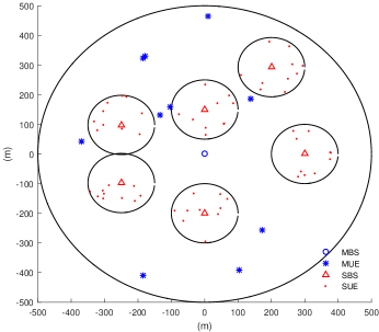
Figure 1: Topology of the small cell network.

VI Numerical Results

In this section, we evaluate the performance of the proposed GNEP methods via numerical simulations. The MBS has $N=10$ channels shared with $M=6$ SBSs, where each channel is allocated to one MUE and one SUE in each macrocell and small cell, respectively, i.e., there are $10$ MUEs and $60$ SUEs. The radii of the macrocell and the small cells are 500m and 100m, respectively. The SBSs and MUEs are randomly and uniformly located within the macrocell, and the SUEs are randomly and uniformly located within each small cell, as shown in Fig. 1. According to [39], the path loss is given by $128.1+37.6\log_{10}d$ dB, where $d$ is the distance in kilometers. The small-scale fading coefficients follow independent and identical zero-mean unit-variance complex Gaussian distributions. We assume that only the total (sum) power budgets are limited, which, from [39], are set to $p_{0}^{\mathrm{sum}}=46$dBm for the MBS and $p_{i}^{\mathrm{sum}}=33$dBm for SBSs $i=1,...,M$. The noise power is $-114$dBm, corresponding to a bandwidth of 10MHz and a noise power spectral density of $-174$dBm.

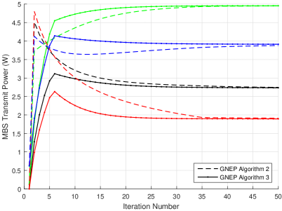
Figure 2: Convergence process of the transmit powers of the MBS for the two GNEP algorithms.

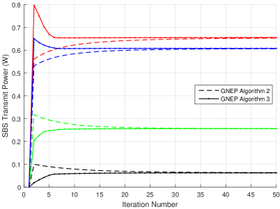
Figure 3: Convergence process of the transmit powers of one SBS for the two GNEP algorithms.

For clarity, we refer to Algorithms 2 and 3 in Section IV as the GNEP methods since they aim to achieve a GNE of $\mathcal{G}$, and to Algorithms 4 and 5 in Section V as the NUM GNEP methods since they aim to achieve a stationary solution of NUM problem $\mathcal{P}$. The proposed methods are compared with two NEP-based distributed methods, namely the NEP and QoS NEP methods. The NEP method [16] is obtained by removing the global QoS constraints from $\mathcal{G}$. In the QoS NEP method [17, 18], the global QoS constraints are replaced by the individual QoS constraints $h_{i0}(n)p_{i}(n)\leq\zeta_{i,n}$ for each SBS $i$ on channel $n$, where the individual QoS threshold is set to $\zeta_{i,n}=(\tilde{h}_{00}(n)p_{0}(n)-\sigma_{0}(n))/M$ for $i=1,\ldots,M$ with $p_{0}(n)=p_{0}^{\mathrm{sum}}/N$. We also compare the proposed methods with the interior point method [38], i.e., a centralized optimization method, which can provide a stationary solution to NUM problem $\mathcal{P}$.

In Figs. 2 and 3, we display the convergence process of the transmit powers for the two GNEP methods, i.e., Algorithms 2 and 3, versus the iteration number with QoS threshold $\gamma_{n}=2$ nats/s/Hz. Due to the large number of users, only the transmit powers of four channels of the MBS and one SBS are shown. One can observe that both algorithms converge rapidly to the same power allocation profile, indicating that they achieve the same GNE. Compared to Algorithm 2, Algorithm 3 converges relatively faster, which is the benefit of simultaneously updating transmit power and price. On the other hand, Algorithm 2 enjoys the advantage of less signaling overhead, since it requires the MBS to broadcast the price less frequently. This corresponds to the commonly-observed tradeoff between convergence and information exchange in distributed optimization.

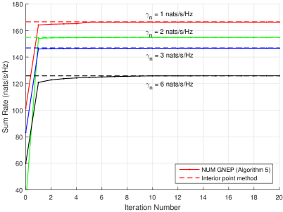
Figure 4: Convergence process of the sum rate of all BSs for the NUM GNEP and interior point methods.

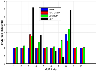
Figure 5: Rate of each MUE with QoS threshold $\gamma_{n}=2$ nats/s/Hz.

Fig. 4 shows the convergence process of the sum rate for the NUM GNEP method, i.e., Algorithm 5, versus the iteration number for different QoS requirements. As indicated in Section V, by properly choosing the algorithm parameters, Algorithm 5 is always guaranteed to converge to a stationary solution of $\mathcal{P}$. This is verified in Fig. 4, where Algorithm 5 converges to the same point as the interior point method. Note that the interior point method is centralized and requires the collection of the channel state information of the entire network at a central node, whereas the NUM GNEP method can be implemented in a decentralized manner with limited signaling overhead.

In Fig. 5, we show the rates of the MUEs generated by different distributed methods with a QoS threshold of $\gamma_{n}=2$ nats/s/Hz for each MUE. The first observation is that the NEP method may violate the QoS requirement and even result in zero rate for some MUEs, i.e., it is not able to protect the macrocell communication. The second observation is that, upon satifying the QoS requirement, the GNEP and the NUM GNEP methods tend to meet exactly the QoS threshold, whereas the QoS NEP method often leads to MUE rates higher than the QoS threshold. From the system perspective, such redundancy in QoS satisfaction may come at the expense of a degradation of the performance of other utilities. e.g., the sum rate, of the BSs.

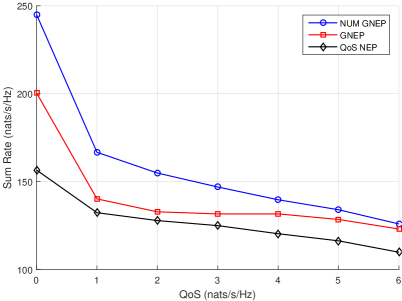
Figure 6: Sum rate versus QoS threshold.

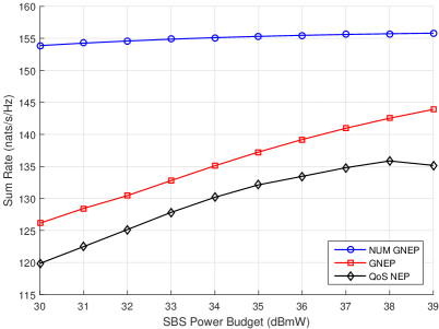
Figure 7: Sum rate versus SBS power budget.

To further elaborate on this point, we plot the sum rate versus the QoS threshold in Fig. 6 and the sum rate versus the total power budget of the SBSs with a QoS threshold of $\gamma_{n}=2$ nats/s/Hz in Fig. 7. As can be observed from both figures, the GNEP method achieves a higher sum rate than the QoS NEP method. This is because the global QoS constraints allow to control the aggregate interference at each MUE in a more flexible manner than the individual QoS constraints and hence provide more degrees of freedom for improving the network utility.

As expected, the NUM GNEP method, which aims to maximize the sum rate of all BSs under the QoS constraints, achieves the highest sum rate. The cost of the gain compared to the GNEP method is a higher signaling overhead between the BSs as well as a higher complexity. Indeed, Figs. 6 and 7 demonstrate the fundamental tradeoff between signaling overhead and network performance, i.e., the more signaling overhead can be afforded, the better the achievable network performance. The proposed GNEP framework is able to flexibly adjust this tradeoff by providing different GNEP-based distributed optimization methods.

VII Conclusions and Extensions

We have considered the interference management of a two-tier hierarchical small cell network and developed a GNEP framework for distributed optimization of the transmit strategies of the SBSs and the MBS. The two different network design philosophies, i.e., achieving a GNE while satisfying global QoS constraints and maximizing the network utility under global QoS constraints, are unified under the GNEP framework. We have developed various GNEP-based distributed algorithms, which differ in the signaling overhead and complexity required to meet the global QoS constraints at the GNE or to obtain a stationary solution to the sum-rate maximization problem. The convergence properties of the proposed algorithms were investigated.

The established GNEP framework can be extended in the following directions. 1) Multiple MBSs: Each MBS can logically view other MBSs as SBSs and all BSs still play the same GNEP. 2) Global QoS constraints for SUEs: the SBS, whose SUEs have global QoS requirements, can be logically viewed as an MBS, which then falls into the case of multiple MBSs. 3) Other utilities: Each MBS or SBS can adopt utilities other than the information rate as long as the utility is concave in its own variables. The best response and convergence properties can be derived using similar steps as in this paper.

The mathematical results derived in this paper guarantee that the global QoS constraints are satisfied and a stationary solution is obtained when the algorithms converge. Nevertheless, in practice, one can terminate the algorithms before convergence (which is equivalent to using a lower precision in the algorithms) and still obtain a close-to-optimal performance. This and the aforementioned extensions make the desired results applicable to a wide range of network scenarios including dense and hyper-dense small cell networks.

-A A Brief Introduction to VI Theory

We first introduce the basic concepts of VIs and generalized VIs (GVIs). Specifically, let $\mathcal{X}\in\mathbb{R}^{n}$ and $\mathbf{F}:\mathcal{X}\rightarrow\mathbb{R}^{n}$ be a continuous function. Then, a VI problem, denoted by $\mathrm{VI}(\mathcal{X},\mathbf{F})$, is to find a vector $\mathbf{x}^{\star}\in\mathcal{X}$ such that $(\mathbf{x}-\mathbf{x}^{\star})^{T}\mathbf{F}(\mathbf{x}^{\star})\geq 0$, $\forall\mathbf{x}\in\mathcal{X}$. More generally, if $\mathbf{F}(\mathbf{x})$ is a point-to-set map $\mathcal{F}(\mathbf{x})\subseteq\mathbb{R}^{n}$ (also referred to as a set-valued function), then we have a GVI. Specifically, let $\mathcal{X}\in\mathbb{R}^{n}$ and $\mathcal{F}:\mathcal{X}\rightarrow\mathbb{R}^{n}$ be a point-to-set map. Then, a GVI problem, denoted by $\mathrm{GVI}(\mathcal{X},\mathcal{F})$, is to find a vector $\mathbf{x}^{\star}\in\mathcal{X}$ such that there exists a vector $\mathbf{z}^{\star}\in\mathcal{F}(\mathbf{x}^{\star})$ and $(\mathbf{x}-\mathbf{x}^{\star})^{T}\mathbf{z}^{\star}\geq 0$, $\forall\mathbf{x}\in\mathcal{X}$.

In VI theory, a function $\mathbf{F}$ is monotone on $\mathcal{X}$ if for any distinct vectors $\mathbf{x},\mathbf{y}\in\mathcal{X}$, $(\mathbf{x}-\mathbf{y})^{T}(\mathbf{F}(\mathbf{x})-\mathbf{F}(\mathbf{y}))\geq 0,$ and strongly monotone if there exists a constant $c_{\mathrm{sm}}>0$ such that for any distinct vectors $\mathbf{x},\mathbf{y}\in\mathcal{X}$, $\left(\mathbf{x}-\mathbf{y}\right)^{T}\left(\mathbf{F}(\mathbf{x})-\mathbf{F}(\mathbf{y})\right)\geq c_{\mathrm{sm}}\left\|\mathbf{x}-\mathbf{y}\right\|^{2}$. A function $\mathbf{F}\triangleq\left(\mathbf{F}_{k}\right)_{k=1}^{K}$ is uniformly P on $\mathcal{X}=\prod_{k=1}^{K}\mathcal{X}_{k}$ if there exists a constant $c_{\mathrm{up}}>0$ such that for any distinct vectors $\mathbf{x}=(\mathbf{x}_{k})_{k=1}^{K}$ and $\mathbf{y}=(\mathbf{y}_{k})_{k=1}^{K}\in\mathcal{X}$, $\max_{k=1,\ldots,K}\left(\mathbf{x}_{k}-\mathbf{y}_{k}\right)^{T}\left(\mathbf{F}_{k}(\mathbf{x})-\mathbf{F}_{k}(\mathbf{y})\right)\geq c_{\mathrm{up}}\left\|\mathbf{x}-\mathbf{y}\right\|^{2}$. $\mathrm{VI}(\mathcal{X},\mathbf{F})$ is monotone, strongly monotone, and uniformly P if $\mathbf{F}$ is monotone, strongly monotone, and uniformly P on $\mathcal{X}$, respectively. Note that the uniformly P property and strong monotonicity often imply a unique solution to a VI (or GVI) [23].

Related to the (strong) monotonicity and uniformly P property of VIs are several special matrix definitions. A matrix $\mathbf{A}\in\mathbb{R}^{n\times n}$ is a Z-matrix if its off-diagonal entries are all non-positive and a P-matrix if all its principle minors are positive. A Z-matrix that is also a P-matrix is a K-matrix. These matrices have the following properties.

Lemma 10.

([40]) A matrix $\mathbf{A}\in\mathbb{R}^{n\times n}$ is a P-matrix if and only if $\mathbf{A}$ does not invert the sign of any non-zero vector, i.e., if $x_{i}[\mathbf{A}\mathbf{x}]_{i}\leq 0$ for $\forall i$, then $\mathbf{x}$ is an all-zero vector.

Lemma 11.

([40]) Let $\mathbf{A}\in\mathbb{R}^{n\times n}$ be a K-matrix and $\mathbf{B}$ a non-negative matrix. Then, $\rho(\mathbf{A}^{-1}\mathbf{B})<1$ if and only if $\mathbf{A}-\mathbf{B}$ is a K-matrix.

-B Proof of Proposition 1

The existence of a solution of $\mathrm{VI}(\mathcal{S},\mathbf{f})$ follows directly from [23, Corollary 2.2.5]. Next, we show that $\mathbf{f}(\mathbf{p})$ is uniformly P on $\mathcal{S}$ if $\mathbf{\Psi}$ is a P-matrix, which leads to a unique solution.

Consider two distinct vectors $\mathbf{p}^{1}\triangleq(\mathbf{p}_{i}^{1})_{i=0}^{M},\mathbf{p}^{2}\triangleq(\mathbf{p}_{i}^{2})_{i=0}^{M}\in\mathcal{\mathcal{S}}$ and define $z_{i}(\theta)$ with $\theta\in[0,1]$

$$z_{i}(\theta)=\left(\mathbf{p}_{i}^{1}-\mathbf{p}_{i}^{2}\right)^{T}\mathbf{f}_{i}\left(\theta\mathbf{p}^{1}+(1-\theta)\mathbf{p}^{2}\right).$$ (27)

From the mean value theorem, the derivative of $z_{i}(\theta)$ with respect to some $\theta\in[0,1]$ is given by

$$z_{i}^{\prime}(\theta)=z_{i}(1)-z_{i}(0)=\left(\mathbf{p}_{i}^{1}-\mathbf{p}_{i}^{2}\right)^{T}\left(\mathbf{f}_{i}(\mathbf{p}^{1})-\mathbf{f}_{i}(\mathbf{p}^{2})\right).$$ (28)

On the other hand, $z_{i}^{\prime}(\theta)$ can be calculated as

$$z_{i}^{\prime}(\theta) =\left(\mathbf{p}_{i}^{1}-\mathbf{p}_{i}^{2}\right)^{T}\sum_{j=0}^{M}\nabla_{\mathbf{p}_{j}}\mathbf{f}_{i}(\mathbf{p}_{\theta})\left(\mathbf{p}_{j}^{1}-\mathbf{p}_{j}^{2}\right)$$

$$=\mathbf{d}_{i}^{T}\sum_{j=0}^{M}\nabla_{\mathbf{p}_{j}}\mathbf{f}_{i}(\mathbf{p}_{\theta})\mathbf{d}_{j}$$

$$\geq\mathbf{d}_{i}^{T}\nabla_{\mathbf{p}_{i}}\mathbf{f}_{i}(\mathbf{p}_{\theta})\mathbf{d}_{i}-\sum_{j\neq i}\left|\mathbf{d}_{i}^{T}\nabla_{\mathbf{p}_{j}}\mathbf{f}_{i}(\mathbf{p}_{\theta})\mathbf{d}_{j}\right|$$ (29)

where $\mathbf{d}_{j}\triangleq\mathbf{p}_{j}^{1}-\mathbf{p}_{j}^{2}$ and $\mathbf{p}_{\theta}\triangleq\theta\mathbf{p}^{1}+(1-\theta)\mathbf{p}^{2}\in\mathcal{\mathcal{S}}$ since $\mathcal{\mathcal{S}}$ is a convex set.

It is not difficult to verify that $\nabla_{\mathbf{p}_{j}}\mathbf{f}_{i}(\mathbf{p})=-\nabla_{\mathbf{p}_{i}\mathbf{p}_{j}}^{2}R_{i}(\mathbf{p})$ is an $N\times N$ diagonal matrix with diagonal elements

$$h_{ii}(n)h_{ji}(n)\left(\sigma_{i}(n)+\sum_{l=0}^{M}h_{li}(n)p_{l}(n)\right)^{-2}\leq\\ h_{ii}(n)h_{ji}(n)\sigma_{i}^{-2}(n)\triangleq\beta_{ij}(n)$$ (30)

and $\nabla_{\mathbf{p}_{i}}\mathbf{f}_{i}(\mathbf{p})=-\nabla_{\mathbf{p}_{i}}^{2}R_{i}(\mathbf{p})$ is also an $N\times N$ diagonal matrix with diagonal elements

$$h_{ii}^{2}(n)\left(\sigma_{i}(n)+\sum_{l=0}^{M}h_{li}(n)p_{l}(n)\right)^{-2}\geq\\ h_{ii}^{2}(n)\left(\sigma_{i}(n)+\sum_{l=0}^{M}h_{li}(n)p_{l,n}^{\mathrm{max}}\right)^{-2}\triangleq\alpha_{i}(n)$$ (31)

where $p_{l,n}^{\mathrm{max}}\triangleq\min\left\{p_{l}^{\mathrm{sum}},p_{l,n}^{\mathrm{peak}}\right\}$. Let $\alpha_{i}^{\mathrm{min}}\triangleq\min_{n}\{\alpha_{i}(n)\}$ and $\beta_{ij}^{\mathrm{max}}\triangleq\max_{n}\{\beta_{ij}(n)\}$. Then, we have $\mathbf{d}_{i}^{T}\nabla_{\mathbf{p}_{i}}\mathbf{f}_{i}(\mathbf{p}_{\theta})\mathbf{d}_{i}\geq\alpha_{i}^{\mathrm{min}}\left\|\mathbf{d}_{i}\right\|^{2}$ and

$$\left|\mathbf{d}_{i}^{T}\nabla_{\mathbf{p}_{j}}\mathbf{f}_{i}(\mathbf{p}_{\theta})\mathbf{d}_{j}\right|\leq\left\|\mathbf{d}_{i}\right\|\left\|\nabla_{\mathbf{p}_{j}}\mathbf{f}_{i}(\mathbf{p}_{\theta})\mathbf{d}_{j}\right\|\leq\beta_{ij}^{\mathrm{max}}\left\|\mathbf{d}_{i}\right\|\left\|\mathbf{d}_{j}\right\|.$$ (32)

Consequently, we obtain

$$z_{i}^{\prime}(\theta) \geq\alpha_{i}^{\mathrm{min}}\left\|\mathbf{d}_{i}\right\|^{2}-\sum_{j\neq i}\beta_{ij}^{\mathrm{max}}\left\|\mathbf{d}_{i}\right\|\left\|\mathbf{d}_{j}\right\|$$

$$=\alpha_{i}^{\mathrm{min}}s_{i}^{2}-\sum_{j\neq i}\beta_{ij}^{\mathrm{max}}s_{j}s_{i}=s_{i}\left[\mathbf{\Psi}\mathbf{s}\right]_{i}$$ (33)

where $s_{j}\triangleq\left\|\mathbf{d}_{j}\right\|$, $\mathbf{s}\triangleq\left(s_{j}\right)_{j=0}^{M}$, and $\mathbf{\Psi}$ is defined as in (10). Combining (28) and (33), we have

$$\left(\mathbf{p}_{i}^{1}-\mathbf{p}_{i}^{2}\right)^{T}\left(\mathbf{f}_{i}(\mathbf{p}^{1})-\mathbf{f}_{i}(\mathbf{p}^{2})\right)\geq s_{i}\left[\mathbf{\Psi}\mathbf{s}\right]_{i}>0$$ (34)

where the last inequality follows from Lemma 10 in Appendix -A, since $\mathbf{\Psi}$ is a P-matrix. Therefore, there always exists a constant $c_{\mathrm{up}}$ such that $\max_{i}\left(\mathbf{p}_{i}^{1}-\mathbf{p}_{i}^{2}\right)^{T}\left(\mathbf{f}_{i}(\mathbf{p}^{1})-\mathbf{f}_{i}(\mathbf{p}^{2})\right)\geq c_{\mathrm{up}}\left\|\mathbf{p}^{1}-\mathbf{p}^{2}\right\|^{2}$, which proves $\mathbf{f}(\mathbf{p})$ is a uniformly P function.

-C Proof of Proposition 3

From Lemma 3, $\mathbf{p}^{\star}$ is a NE of $\mathcal{G}_{\boldsymbol{\mu}}$ if and only if

$$\left(\mathbf{p}_{i}-\mathbf{p}_{i}^{\star}\right)^{T}\mathbf{f}_{\boldsymbol{\mu},i}(\mathbf{p}_{i}^{\star},\mathbf{p}_{-i}^{\star})\geq 0,\quad\forall\mathbf{p}_{i}\in\mathcal{S}_{i}^{\mathrm{pow}}.$$ (35)

From the first-order optimality condition, the best response $\mathbf{p}_{i}^{t+1}$ is a solution to (12) with $\mathbf{p}_{-i}=\mathbf{p}_{-i}^{t}$ if and only if

$$\left(\mathbf{p}_{i}-\mathbf{p}_{i}^{t+1}\right)^{T}\mathbf{f}_{\boldsymbol{\mu},i}(\mathbf{p}_{i},\mathbf{p}_{-i}^{t})\geq 0,\quad\forall\mathbf{p}_{i}\in\mathcal{S}_{i}^{\mathrm{pow}}.$$ (36)

Adding (35) with $\mathbf{p}_{i}=\mathbf{p}_{i}^{t+1}$ and (36) with $\mathbf{p}_{i}=\mathbf{p}_{i}^{\star}$, we have

$$\left(\mathbf{p}_{i}^{t+1}-\mathbf{p}_{i}^{\star}\right)^{T}\left(\mathbf{f}_{\boldsymbol{\mu},i}(\mathbf{p}_{i}^{\star},\mathbf{p}_{-i}^{\star})-\mathbf{f}_{\boldsymbol{\mu},i}(\mathbf{p}_{i}^{t+1},\mathbf{p}_{-i}^{t})\right) =$$

$$\left(\mathbf{p}_{i}^{t+1}-\mathbf{p}_{i}^{\star}\right)^{T}\left(\mathbf{f}_{i}(\mathbf{p}_{i}^{\star},\mathbf{p}_{-i}^{\star})-\mathbf{f}_{i}(\mathbf{p}_{i}^{t+1},\mathbf{p}_{-i}^{t})\right) \geq 0$$ (37)

where the equality follows from the definition of $\mathbf{f}_{\boldsymbol{\mu},i}$ in (14).

Let $\mathbf{p}_{\theta}\triangleq\theta\left(\mathbf{p}_{i}^{\star},\mathbf{p}_{-i}^{\star}\right)+(1-\theta)\left(\mathbf{p}_{i}^{t+1},\mathbf{p}_{-i}^{t}\right)$. It then follows from (27)-(29) and (33) that for some $\theta\in[0,1]$

$$0\leq \left(\mathbf{p}_{i}^{t+1}-\mathbf{p}_{i}^{\star}\right)^{T}\left(\nabla_{\mathbf{p}_{i}}\mathbf{f}_{i}(\mathbf{p}_{\theta})(\mathbf{p}_{i}^{\star}-\mathbf{p}_{i}^{t+1})\right.$$

$$+\sum_{j\neq i}\nabla_{\mathbf{p}_{j}}\mathbf{f}_{i}(\mathbf{p}_{\theta})\left.(\mathbf{p}_{j}^{\star}-\mathbf{p}_{j}^{t})\right)$$

$$= -(\mathbf{d}_{i}^{t+1})^{T}\nabla_{\mathbf{p}_{i}}\mathbf{f}_{i}(\mathbf{p}_{\theta})\mathbf{d}_{i}^{t+1}-\sum_{j\neq i}(\mathbf{d}_{i}^{t+1})^{T}\nabla_{\mathbf{p}_{j}}\mathbf{f}_{i}(\mathbf{p}_{\theta})\mathbf{d}_{j}^{t}$$

$$\leq -\alpha_{i}^{\mathrm{min}}\left\|\mathbf{d}_{i}^{t+1}\right\|^{2}+\sum_{j\neq i}\beta_{ij}^{\mathrm{max}}\left\|\mathbf{d}_{i}^{t+1}\right\|\left\|\mathbf{d}_{j}^{t}\right\|.$$ (38)

where $\mathbf{d}_{i}^{t}\triangleq\mathbf{p}_{i}^{t}-\mathbf{p}_{i}^{\star}$, and $\alpha_{i}^{\mathrm{min}}$ and $\beta_{ij}^{\mathrm{max}}$ are defined after (31). Introducing $s_{i}^{t}\triangleq\left\|\mathbf{d}_{i}^{t}\right\|$ and $\mathbf{s}^{t}\triangleq(s_{i}^{t})_{i=0}^{M}$, we obtain $s_{i}^{t+1}\leq\frac{1}{\alpha_{i}^{\mathrm{min}}}\sum_{j\neq i}\beta_{ij}^{\mathrm{max}}s_{j}^{t}$, which, from the definition of $\mathbf{\Phi}$ in (11), implies $\mathbf{s}^{t+1}\leq\mathbf{\Phi}\mathbf{s}^{t}$. Therefore, the error sequence $\left\{\mathbf{s}^{t}\right\}$ converges to zero if $\rho\left(\mathbf{\Phi}\right)<1$, which, from Lemma 2, is equivalent to $\mathbf{\Psi}$ being a P-matrix.

-D Proof of Lemma 7

The optimal $p_{i}^{\star}(n)$ is obtained by taking the derivative of the objective in (20), leading to

$$\frac{h_{00}(n)}{h_{00}(n)p_{0}(n)+I_{0,n}(\mathbf{p}_{-0})}-cp_{0}(n)+cp_{0}^{k}(n)+\mu_{n}\tilde{h}_{00}(n)=\lambda_{0}$$

$$\frac{h_{ii}(n)}{h_{ii}(n)p_{i}(n)+I_{i,n}(\mathbf{p}_{-i})}-cp_{i}(n)+cp_{i}^{k}(n)-\mu_{n}h_{i0}(n)=\lambda_{i}$$

for $i=1,\ldots,M$. It is easily seen that $\lambda_{i}$ is monotonically nonincreasing in $p_{i}(n)$. Since the projection does not change the monotonicity, Lemma 7 is thus proved.

-E Proof of Proposition 4

Since $\mathbf{f}_{\mathbf{p}^{u}}(\mathbf{p})=\left(-\nabla_{\mathbf{p}_{i}}R_{i}(\mathbf{p})+\mathbf{b}_{i}(\mathbf{p}^{u})\right)_{i=0}^{M}$, if $\mathbf{p}^{\star}=\mathrm{VE}(\mathbf{p}^{\star})$, it follows that

$$(\mathbf{p}-\mathbf{p}^{\star})^{T}\mathbf{f}_{\mathbf{p}^{\star}}(\mathbf{p}^{\star}) =\sum_{i=0}^{M}(\mathbf{p}_{i}-\mathbf{p}_{i}^{\star})^{T}\left(-\nabla_{\mathbf{p}_{i}}R_{i}(\mathbf{p}^{\star})+\mathbf{b}_{i}(\mathbf{p}^{\star})\right)$$

$$=\sum_{i=0}^{M}(\mathbf{p}_{i}-\mathbf{p}_{i}^{\star})^{T}\left(-\sum_{j=0}^{M}\nabla_{\mathbf{p}_{i}}R_{j}(\mathbf{p}^{\star})\right)$$

$$=-\sum_{j=0}^{M}(\mathbf{p}-\mathbf{p}^{\star})^{T}\nabla_{\mathbf{p}}R_{j}(\mathbf{p}^{\star})\geq 0$$

which is equivalent to the first-order optimality condition of $\mathcal{P}$, implying $\mathbf{p}^{\star}$ is a stationary point of $\mathcal{P}$. Conversely, if $\mathbf{p}^{\star}$ is a stationary point of $\mathcal{P}$, we also obtain $\mathbf{p}^{\star}=\mathrm{VE}(\mathbf{p}^{\star})$.

-F Proof of Theorem 4

Consider two distinct points $\mathbf{p}^{1},\mathbf{p}^{2}\in\mathcal{S}$, and let $\mathbf{z}^{1}=\mathrm{VE}(\mathbf{p}^{1})$ and $\mathbf{z}^{2}=\mathrm{VE}(\mathbf{p}^{2})$. Then, we have for $\forall\mathbf{p}\in\mathcal{S}$, $\forall i$

$$(\mathbf{p}_{i}-\mathbf{z}_{i}^{1})^{T}\left(\mathbf{f}_{i}(\mathbf{z}^{1})+\mathbf{b}_{i}(\mathbf{p}^{1})\right) \geq 0$$ (39)

$$(\mathbf{p}_{i}-\mathbf{z}_{i}^{2})^{T}\left(\mathbf{f}_{i}(\mathbf{z}^{2})+\mathbf{b}_{i}(\mathbf{p}^{2})\right) \geq 0.$$ (40)

By adding (39) with $\mathbf{p}_{i}=\mathbf{z}_{i}^{2}$ to (40) with $\mathbf{p}_{i}=\mathbf{z}_{i}^{1}$, we obtain $(\mathbf{z}_{i}^{1}-\mathbf{z}_{i}^{2})^{T}(\mathbf{f}_{i}(\mathbf{z}^{2})-\mathbf{f}_{i}(\mathbf{z}^{1})+\mathbf{b}_{i}(\mathbf{p}^{2})-\mathbf{b}_{i}(\mathbf{p}^{1}))\geq 0$ or equivalently $(\mathbf{z}_{i}^{1}-\mathbf{z}_{i}^{2})^{T}\left(\mathbf{b}_{i}(\mathbf{p}^{2})-\mathbf{b}_{i}(\mathbf{p}^{1})\right)\geq(\mathbf{z}_{i}^{1}-\mathbf{z}_{i}^{2})^{T}\left(\mathbf{f}_{i}(\mathbf{z}^{1})-\mathbf{f}_{i}(\mathbf{z}^{2})\right)$. It follows from (34) that

$$(\mathbf{z}_{i}^{1}-\mathbf{z}_{i}^{2})^{T}\left(\mathbf{f}_{i}(\mathbf{z}^{1})-\mathbf{f}_{i}(\mathbf{z}^{2})\right)\geq s_{i}\left[\mathbf{\Psi}\mathbf{s}\right]_{i}$$ (41)

where $s_{i}\triangleq\left\|\mathbf{z}_{i}^{1}-\mathbf{z}_{i}^{2}\right\|$ and $\mathbf{s}\triangleq(s_{i})_{i=0}^{M}$.

Using the mean value theorem as in (29), we have for some $\theta\in[0,1]$ and $\mathbf{p}_{\theta}\triangleq\theta\mathbf{p}^{2}+(1-\theta)\mathbf{p}^{1}\in\mathcal{\mathcal{S}}$

$$(\mathbf{z}_{i}^{1}-\mathbf{z}_{i}^{2})^{T}\left(\mathbf{b}_{i}(\mathbf{p}^{2})-\mathbf{b}_{i}(\mathbf{p}^{1})\right)$$

$$=\left(\mathbf{z}_{i}^{1}-\mathbf{z}_{i}^{2}\right)^{T}\sum_{j=0}^{M}\nabla_{\mathbf{p}_{j}}\mathbf{b}_{i}(\mathbf{p}_{\theta})(\mathbf{p}_{j}^{2}-\mathbf{p}_{j}^{1})$$

$$\leq\sum_{j=0}^{M}\left\|\mathbf{z}_{i}^{1}-\mathbf{z}_{i}^{2}\right\|\left\|\nabla_{\mathbf{p}_{j}}\mathbf{b}_{i}(\mathbf{p}_{\theta})(\mathbf{p}_{j}^{2}-\mathbf{p}_{j}^{1})\right\|$$

$$\leq\left\|\mathbf{z}_{i}^{1}-\mathbf{z}_{i}^{2}\right\|\sum_{j=0}^{M}\left\|\mathbf{p}_{j}^{2}-\mathbf{p}_{j}^{1}\right\|\sup_{\mathbf{p}_{\theta}}\left\|\nabla_{\mathbf{p}_{j}}\mathbf{b}_{i}(\mathbf{p}_{\theta})\right\|_{2}.$$ (42)

Although complicated, it can be verified that for $\forall i,j$

$$\left[\mathbf{\Upsilon}\right]_{ij}\geq\sup_{\mathbf{p}_{\theta}}\left\|\nabla_{\mathbf{p}_{j}}\mathbf{b}_{i}(\mathbf{p}_{\theta})\right\|_{2}.$$ (43)

Let $\mathbf{e}\triangleq(e_{j})_{j=0}^{M}$ with $e_{j}\triangleq\left\|\mathbf{p}_{j}^{1}-\mathbf{p}_{j}^{2}\right\|$. It follows from (41)-(43) that $\sum_{j=0}^{M}\left[\mathbf{\Upsilon}\right]_{ij}e_{j}=\left[\mathbf{\Upsilon}\mathbf{e}\right]_{i}\geq\left[\mathbf{\Psi}\mathbf{s}\right]_{i}$, which leads to $\mathbf{\Psi}\mathbf{s}\leq\mathbf{\Upsilon}\mathbf{e}$. Since $\left\|\mathbf{s}\right\|=\left\|\mathbf{z}^{1}-\mathbf{z}^{2}\right\|$ and $\left\|\mathbf{e}\right\|=\left\|\mathbf{p}^{1}-\mathbf{p}^{2}\right\|$, $\mathbf{z}=\mathrm{VE}(\mathbf{p})$ is a contraction mapping if $\rho(\mathbf{\Psi}^{-1}\mathbf{\Upsilon})<1$. To guarantee the convergence of Algorithms 2 and 3 as well as the invertibility of $\mathbf{\Psi}$, we also require $\mathbf{\Psi}\succ\mathbf{0}$.

-G Proof of Proposition 5

Similar to Proposition 4, given $\mathbf{q}^{v}$, if $\mathbf{p}^{u+1}=\mathrm{VE}(\mathbf{p}^{u},\mathbf{q}^{v})$ converges to $\mathbf{p}_{\mathbf{q}^{v}}^{\star}$, it must be a stationary point of $\mathcal{P}_{\mathbf{q}^{v}}$. Next, we prove the convergence of $\mathbf{p}^{u+1}=\mathrm{VE}(\mathbf{p}^{u},\mathbf{q}^{v})$.

$\mathrm{VE}(\mathbf{p}^{u},\mathbf{q}^{v})$ is the solution of $\mathrm{VI}(\mathcal{S},\mathbf{f}_{\mathbf{p}^{u},\mathbf{q}^{v}})$ with $\mathbf{f}_{\mathbf{p}^{u}}(\mathbf{p})\triangleq\mathbf{f}(\mathbf{p})+\mathbf{b}(\mathbf{p}^{u})+\tau(\mathbf{p}-\mathbf{q}^{v})$. Thus, given $\mathbf{z}^{1}=\mathrm{VE}(\mathbf{p}^{1},\mathbf{q}^{v})$ and $\mathbf{z}^{2}=\mathrm{VE}(\mathbf{p}^{2},\mathbf{q}^{v})$, we have for $\forall\mathbf{p}\in\mathcal{S}$ and $\forall i$

$$(\mathbf{p}_{i}-\mathbf{z}_{i}^{1})^{T}\left(\mathbf{f}_{i}(\mathbf{z}^{1})+\mathbf{b}_{i}(\mathbf{p}^{1})+\tau(\mathbf{z}_{i}^{1}-\mathbf{q}_{i}^{v})\right) \geq 0$$

$$(\mathbf{p}_{i}-\mathbf{z}_{i}^{2})^{T}\left(\mathbf{f}_{i}(\mathbf{z}^{2})+\mathbf{b}_{i}(\mathbf{p}^{2})+\tau(\mathbf{z}_{i}^{2}-\mathbf{q}_{i}^{v})\right) \geq 0$$

which leads to

$$(\mathbf{z}_{i}^{1}-\mathbf{z}_{i}^{2})^{T}\left(\mathbf{b}_{i}(\mathbf{p}^{2})-\mathbf{b}_{i}(\mathbf{p}^{1})\right)$$

$$\geq(\mathbf{z}_{i}^{1}-\mathbf{z}_{i}^{2})^{T}\left(\mathbf{f}_{i}(\mathbf{z}^{1})-\mathbf{f}_{i}(\mathbf{z}^{2})\right)+\tau\left\|\mathbf{z}_{i}^{1}-\mathbf{z}_{i}^{2}\right\|^{2}$$

$$\geq s_{i}\left[\mathbf{\Psi}\mathbf{s}\right]_{i}+\tau s_{i}^{2}$$

where the last equality follows from (34) with $s_{i}\triangleq\left\|\mathbf{z}_{i}^{1}-\mathbf{z}_{i}^{2}\right\|$ and $\mathbf{s}\triangleq(s_{i})_{i=0}^{M}$. Then, using (42) and (43), we have $\left[\mathbf{\Upsilon}\mathbf{e}\right]_{i}\geq\left[\mathbf{\Psi}\mathbf{s}\right]_{i}+\tau s_{i}$, where $e_{i}\triangleq\left\|\mathbf{p}_{i}^{1}-\mathbf{p}_{i}^{2}\right\|$ and $\mathbf{e}\triangleq(e_{i})_{i=0}^{M}$, which leads to $(\tau\mathbf{I}+\mathbf{\Psi})\mathbf{s}\leq\mathbf{\Upsilon}\mathbf{e}$. Thus, $\mathbf{z}=\mathrm{VE}(\mathbf{p},\mathbf{q}^{v})$ is a contraction mapping if $\rho((\tau\mathbf{I}+\mathbf{\Psi})^{-1}\mathbf{\Upsilon})<1$ or equivalently (from Lemma 11) $\tau\mathbf{I}+\mathbf{\Psi}-\mathbf{\Upsilon}$ is a P-matrix, which is implied by $\tau\mathbf{I}+\mathbf{\Psi}-\mathbf{\Upsilon}\succ\mathbf{0}$ and achieved by setting $\tau>\left|\lambda_{\mathrm{min}}\left(\mathbf{\Psi}-\mathbf{\Upsilon}\right)\right|$. Meanwhile, for the convergence of Algorithms 2 and 3, we shall have $\tau\mathbf{I}+\mathbf{\Psi}\succ\mathbf{0}$, which is implied by the strict diagonal dominance, i.e., $\tau+\left[\mathbf{\Psi}\right]_{ii}>\sum_{j\neq i}\left[\left|\mathbf{\Psi}\right|\right]_{ij}$, $\forall i$ and $\tau+\left[\mathbf{\Psi}\right]_{jj}>\sum_{i}\left[\left|\mathbf{\Psi}\right|\right]_{ij}$, $\forall j$. Therefore, we have $\tau>\max\{\max_{i}(\sum_{j\neq i}\left[\left|\mathbf{\Psi}\right|\right]_{ij}-\left[\mathbf{\Psi}\right]_{ii}),\max_{j}(\sum_{i}\left[\left|\mathbf{\Psi}\right|\right]_{ij}-\left[\mathbf{\Psi}\right]_{jj})\}$.

-H Proof of Lemma 8

Since $\nabla_{\mathbf{p}_{i}}F_{\tau}(\mathbf{p})=\mathbf{f}_{i}(\mathbf{p})+\mathbf{b}_{i}(\mathbf{p})+\tau(\mathbf{p}_{i}-\mathbf{q}_{i}^{v})$, we have

$$(\mathbf{p}^{1}-\mathbf{p}^{2})^{T}(\nabla_{\mathbf{p}}F_{\tau}(\mathbf{p}^{1})-\nabla_{\mathbf{p}}F_{\tau}(\mathbf{p}^{2}))=\sum_{i=0}^{M}\tau\left\|\mathbf{p}_{i}^{1}-\mathbf{p}_{i}^{2}\right\|^{2}\\ +\sum_{i=0}^{M}(\mathbf{p}_{i}^{1}-\mathbf{p}_{i}^{2})^{T}\left(\mathbf{f}_{i}(\mathbf{p}^{1})-\mathbf{f}_{i}(\mathbf{p}^{2})+\mathbf{b}_{i}(\mathbf{p}^{1})-\mathbf{b}_{i}(\mathbf{p}^{2})\right).$$

With $\mathbf{d}_{i}\triangleq\mathbf{p}_{i}^{1}-\mathbf{p}_{i}^{2}$ and $s_{i}\triangleq\left\|\mathbf{d}_{i}\right\|$ and from (27)-(29), we have for some $\theta\in[0,1]$ and $\mathbf{p}_{\theta}\triangleq\theta\mathbf{p}^{1}+(1-\theta)\mathbf{p}^{2}\in\mathcal{\mathcal{S}}$

$$(\mathbf{p}_{i}^{1}-\mathbf{p}_{i}^{2})^{T}(\mathbf{b}_{i}(\mathbf{p}^{1})-\mathbf{b}_{i}(\mathbf{p}^{2})$$

$$\geq\mathbf{d}_{i}^{T}\nabla_{\mathbf{p}_{i}}\mathbf{b}_{i}(\mathbf{p}_{\theta})\mathbf{d}_{i}-\sum_{j\neq i}\left|\mathbf{d}_{i}^{T}\nabla_{\mathbf{p}_{j}}\mathbf{b}_{i}(\mathbf{p}_{\theta})\mathbf{d}_{j}\right|$$

$$\geq s_{i}^{2}\inf_{\mathbf{p}_{\theta}}\lambda_{\mathrm{min}}\left(\nabla_{\mathbf{p}_{i}}\mathbf{b}_{i}(\mathbf{p}_{\theta})\right)-\sum_{j\neq i}s_{i}s_{j}\sup_{\mathbf{p}_{\theta}}\left\|\nabla_{\mathbf{p}_{j}}\mathbf{b}_{i}(\mathbf{p}_{\theta})\right\|_{2}.$$

It can be verified that $\inf_{\mathbf{p}_{\theta}}\lambda_{\mathrm{min}}\left(\nabla_{\mathbf{p}_{i}}\mathbf{b}_{i}(\mathbf{p}_{\theta})\right)\geq-\left[\mathbf{\Upsilon}\right]_{ii}$ and $\sup_{\mathbf{p}_{\theta}}\left\|\nabla_{\mathbf{p}_{j}}\mathbf{b}_{i}(\mathbf{p}_{\theta})\right\|\leq\left[\mathbf{\Upsilon}\right]_{ij}$ for $j\neq i$. So, we have $(\mathbf{p}_{i}^{1}-\mathbf{p}_{i}^{2})^{T}\left(\mathbf{b}_{i}(\mathbf{p}^{1})-\mathbf{b}_{i}(\mathbf{p}^{2})\right)\geq-s_{i}\left[\mathbf{\Upsilon}\mathbf{s}\right]_{i}$. Meanwhile, from (34), we also have $(\mathbf{p}_{i}^{1}-\mathbf{p}_{i}^{2})^{T}\left(\mathbf{f}_{i}(\mathbf{p}^{1})-\mathbf{f}_{i}(\mathbf{p}^{2})\right)\geq s_{i}\left[\mathbf{\Psi}\mathbf{s}\right]_{i}$. Consequently, we obtain

$$(\mathbf{p}^{1}-\mathbf{p}^{2})^{T}\left(\nabla_{\mathbf{p}}F_{\tau}(\mathbf{p}^{1})-\nabla_{\mathbf{p}}F_{\tau}(\mathbf{p}^{2})\right)$$

$$\geq\sum_{i=0}^{M}\left(\tau s_{i}^{2}+s_{i}\left[\mathbf{\Psi}\mathbf{s}\right]_{i}-s_{i}\left[\mathbf{\Upsilon}\mathbf{s}\right]_{i}\right)$$

$$=\mathbf{s}^{T}\left(\tau\mathbf{I}+\mathbf{\Psi}-\mathbf{\Upsilon}\right)\mathbf{s}\geq\left\|\mathbf{s}\right\|^{2}\lambda_{\mathrm{min}}\left(\tau\mathbf{I}+\mathbf{\Psi}-\mathbf{\Upsilon}\right).$$

Therefore, $F_{\tau}(\mathbf{p})$ is strongly convex if $\tau\mathbf{I}+\mathbf{\Psi}-\mathbf{\Upsilon}\succ\mathbf{0}$, which is implied by $\tau>\left|\lambda_{\mathrm{min}}\left(\mathbf{\Psi}-\mathbf{\Upsilon}\right)\right|$. The strong convexity constant $L_{\mathrm{sc}}$ in Lemma 8 is then given by $\tau+\lambda_{\mathrm{min}}\left(\mathbf{\Psi}-\mathbf{\Upsilon}\right)$.

-I Proof of Lemma 9

According to the mean value theory, we have for some $\theta\in[0,1]$ and $\mathbf{p}_{\theta}=\theta\mathbf{p}^{1}-(1-\theta)\mathbf{p}^{2}\in\mathcal{S}$ $\left\|\nabla_{\mathbf{p}}F(\mathbf{p}^{1})-\nabla_{\mathbf{p}}F(\mathbf{p}^{2})\right\|\leq\left\|\nabla_{\mathbf{p}}^{2}F(\mathbf{p}_{\theta})\right\|_{2}\left\|\mathbf{p}^{1}-\mathbf{p}^{2}\right\|$. Since $\nabla_{\mathbf{p}}^{2}F(\mathbf{p})=\left[\nabla_{\mathbf{p}_{i}\mathbf{p}_{j}}F(\mathbf{p})\right]_{i,j=0}^{M}=\left[\nabla_{\mathbf{p}_{j}}\mathbf{f}_{i}(\mathbf{p})\right]_{i,j=0}^{M}+\left[\nabla_{\mathbf{p}_{j}}\mathbf{b}_{i}(\mathbf{p})\right]_{i,j=0}^{M}$, it follows that $\left\|\nabla_{\mathbf{p}}^{2}F(\mathbf{p})\right\|_{2}\leq\sigma_{\max}\left(\left[\nabla_{\mathbf{p}_{j}}\mathbf{f}_{i}(\mathbf{p})\right]_{i,j=0}^{M}\right)+\sigma_{\max}\left(\left[\nabla_{\mathbf{p}_{j}}\mathbf{b}_{i}(\mathbf{p})\right]_{i,j=0}^{M}\right)$. Furthermore, we have $\sigma_{\max}\left(\left[\nabla_{\mathbf{p}_{j}}\mathbf{f}_{i}(\mathbf{p})\right]_{i,j=0}^{M}\right)\leq\sigma_{\max}\left(\left[\sigma_{\max}\left(\nabla_{\mathbf{p}_{j}}\mathbf{f}_{i}(\mathbf{p})\right)\right]_{i,j=0}^{M}\right)$. It can be verified that $\sigma_{\max}\left(\nabla_{\mathbf{p}_{j}}\mathbf{f}_{i}(\mathbf{p})\right)\leq\left[\mathbf{\Xi}\right]_{ij}$, implying $\sigma_{\max}\left(\left[\nabla_{\mathbf{p}_{j}}\mathbf{f}_{i}(\mathbf{p})\right]_{i,j=0}^{M}\right)\leq\sigma_{\max}\left(\mathbf{\Xi}\right)$. Similarly, we can also obtain $\sigma_{\max}\left(\left[\nabla_{\mathbf{p}_{j}}\mathbf{b}_{i}(\mathbf{p})\right]_{i,j=0}^{M}\right)\leq\sigma_{\max}\left(\mathbf{\Upsilon}\right)$. Therefore, we have $\left\|\nabla_{\mathbf{p}}^{2}F(\mathbf{p}_{\theta})\right\|_{2}\leq\sigma_{\max}\left(\mathbf{\Xi}\right)+\sigma_{\max}\left(\mathbf{\Upsilon}\right)$, which is the Lipschitz constant.

-J Proof of Theorem 5

Let $\mathbf{p}_{\mathbf{q}^{v}}^{\star}=\mathrm{VE}(\mathbf{p}^{\star},\mathbf{q}^{v})$. The strong convexity in Lemma 8 leads to the following useful results.

Lemma 12.

Given $\tau>\left|\lambda_{\mathrm{min}}\left(\mathbf{\Psi}-\mathbf{\Upsilon}\right)\right|$, it follows that $\left\|\mathbf{p}_{\mathbf{q}^{1}}^{\star}-\mathbf{p}_{\mathbf{q}^{2}}^{\star}\right\|\leq\frac{\tau}{L_{\mathrm{sc}}}\left\|\mathbf{q}^{1}-\mathbf{q}^{2}\right\|$ and $(\mathbf{p}_{\mathbf{q}}^{\star}-\mathbf{q})^{T}\nabla_{\mathbf{p}}F(\mathbf{q})\leq-L_{\mathrm{sc}}\left\|\mathbf{p}_{\mathbf{q}}^{\star}-\mathbf{q}\right\|^{2}$.

Using the descent lemma [41, Prop. A.24] (with $\mathbf{x}=\mathbf{q}^{v}$ and $\mathbf{y}=\kappa_{v}(\mathbf{p}_{\mathbf{q}^{v}}^{\star}-\mathbf{q}^{v})$), we have

$$F(\mathbf{q}^{v+1})\leq F(\mathbf{q}^{v})+\kappa_{v}(\mathbf{p}_{\mathbf{q}^{v}}^{\star}-\mathbf{q}^{v})^{T}\triangledown_{\mathbf{p}}F\left(\mathbf{q}^{v}\right)\\ +\frac{L_{\mathrm{lip}}\kappa_{v}^{2}}{2}\left\|\mathbf{p}_{\mathbf{q}^{v}}^{\star}-\mathbf{q}^{v}\right\|^{2}.$$

It follows from Lemma 12 that

$$F(\mathbf{q}^{v+1})\leq F(\mathbf{q}^{v})+\frac{1}{2}\left(L_{\mathrm{lip}}\kappa_{v}^{2}-2\kappa_{v}L_{\mathrm{sc}}\right)\left\|\mathbf{p}_{\mathbf{q}^{v}}^{\star}-\mathbf{q}^{v}\right\|^{2}.$$

Given $L_{\mathrm{lip}}\kappa_{v}^{2}-2\kappa_{v}L_{\mathrm{sc}}<0$, we have $F(\mathbf{q}^{v+1})\leq F(\mathbf{q}^{v})$, indicating that $\{F(\mathbf{q}^{v})\}$ converges. This implies that

$$\sum_{v=1}^{\infty}\kappa_{v}\left\|\mathbf{p}_{\mathbf{q}^{v}}^{\star}-\mathbf{q}^{v}\right\|^{2}<+\infty.$$

Since $\sum_{v=1}^{\infty}\kappa_{v}=\infty$, we have $\liminf_{v\rightarrow\infty}\left\|\mathbf{p}_{\mathbf{q}^{v}}^{\star}-\mathbf{q}^{v}\right\|=0$. Given $\kappa_{v}<\frac{1}{1+\frac{\tau}{L_{\mathrm{sc}}}}=\frac{\tau+\lambda_{\mathrm{min}}\left(\mathbf{\Psi}-\mathbf{\Upsilon}\right)}{2\tau+\lambda_{\mathrm{min}}\left(\mathbf{\Psi}-\mathbf{\Upsilon}\right)}$, we can further prove that $\lim_{v\rightarrow\infty}\left\|\mathbf{p}_{\mathbf{q}^{v}}^{\star}-\mathbf{q}^{v}\right\|=0$, for which we refer to [42] for details. From Proposition 5, the fixed point is a stationary point of $\mathcal{P}$.

References

- [1] Ericsson, “5G Radio Access, Research, and Vision,” white paper, 2013.
- [2] J. G. Andrews et al., “What will 5G be?” IEEE J. Sel. Areas Commun., vol. 32, no. 6, pp. 1065–1082, Jun. 2014.
- [3] J. G. Andrews, H. Claussen, M. Dohler, S. Rangan, and M. C. Reed, “Femtocells: Past, present, and future,” IEEE J. Sel. Areas Commun., vol. 30, no. 3, pp. 497–508, Apr. 2012.
- [4] E. Hossain, M. Rasti, H. Tabassum, and A. Abdelnasser, “Evolution toward 5G multi-tier cellular wireless networks: An interference management perspective,” IEEE Wireless Commun., vol. 21, no. 3, pp. 118–127, Jun. 2014.
- [5] T. Q. S. Quek et al., Small Cell Networks: Deployment, PHY Techniques, and Resource Management. Cambridge, U.K.: Cambridge Univ. Press, 2013.
- [6] D. Chen, T. Q. S. Quek, and M. Kountouris, “Backhauling in heterogeneous cellular networks: Modeling and tradeoffs,” IEEE Trans. Wireless Commun., vol. 14, no. 6, pp. 3164–3206, Jun. 2015.
- [7] U. Siddique, H. Tabassum, E. Hossain, and D. I. Kim, “Wireless backhauling of 5G small cells: Challenges and solution approaches,” IEEE Wireless Commun., vol. 22, no. 5, pp. 22–31, Oct. 2015.
- [8] V. Chandrasekhar, J. G. Andrews, T. Muharemovic, Z. Shen, and A. Gatherer, “Power control in two-tier femtocell networks,” IEEE Trans. Wireless Commun., vol. 8, no. 8, pp. 4316–4328, Aug. 2007.
- [9] D. T. Ngo, L. B. Le, T. Le-Ngoc, E. Hossain, and D. I. Kim, “Distributed interference management in two-tier CDMA femtocell networks,” IEEE Trans. Wireless Commun., vol. 11, no. 3, pp. 979–989, Mar. 2012.
- [10] V. N. Ha and L. B. Le, “Fair resource allocation for OFDMA femtocell networks with macrocell protection,” IEEE Trans. Veh. Technol., vol. 63, no. 3, pp. 1388–1401, Mar. 2014.
- [11] D. López-Pérez, X. Chu, A. V. Vasilakos, and H. Claussen, “Power minimization based resource allocation for interference mitigation in OFDMA femtocell networks,” IEEE J. Sel. Areas Commun., vol. 32, no. 2, pp. 333–344, Feb. 2014.
- [12] A. Abdelnasser, E. Hossain, and D. I. Kim, “Tier-aware resource allocation in OFDMA macrocell-small cell networks,” IEEE Trans. Wireless Commun., vol. 63, no. 3, pp. 695–710, Mar. 2015.
- [13] R. Ramamonjison and V. K. Bhargava, “Energy efficiency maximization framework in cognitive downlink two-tier networks,” IEEE Trans. Wireless Commun., vol. 14, no. 3, pp. 1468–1479, Mar. 2015.
- [14] A. R. Elsherif, W.-P. Chen, A. Ito, and Z. Ding, “Resource allocation and inter-cell interference management for dual-access small cells,” IEEE J. Sel. Areas Commun., vol. 33, no. 6, pp. 1082–1096, Jun. 2015.
- [15] R. D. Yates, “A framework for uplink power control in cellular radio systems,” IEEE J. Sel. Areas Commun., vol. 13, no. 7, pp. 1341–1347, Sep. 1995.
- [16] W. Yu, G. Ginis, and J. M. Cioffi, “Distributed multiuser power control for digital subscriber lines,” IEEE J. Sel. Areas Commun., vol. 20, no. 5, pp. 1105–1115, Jun. 2002.
- [17] G. Scutari, F. Facchinei, J.-S. Pang, and D. P. Palomar, “Real and complex monotone communication games,” IEEE Trans. Inform. Theory, vol. 60, no. 7, pp. 4197–4231, Jul. 2014.
- [18] J. Wang, G. Scutari, and D. P. Palomar, “Robust MIMO cognitive radio via game theory,” IEEE Trans. Signal Process., vol. 59, no. 3, pp. 1183–1201, Mar. 2011.
- [19] H. Wang, J. Wang, and Z. Ding, “Distributed power control in a two-tier heterogeneous network,” IEEE Trans. Wireless Commun., vol. 14, no. 12, pp. 6509–6523, Dec. 2015.
- [20] Y. Xu, J. Wang, Q. Wu, A. Anpalagan, and Y.-D. Yao, “Opportunistic spectrum access in unknown dynamic environment: A game-theoretic stochastic learning solution,” IEEE Trans. Wireless Commun., vol. 11, no. 4, pp. 1380–1391, Apr. 2012.
- [21] S. Guruacharya, D. Niyato, D. I. Kim, and E. Hossain, “Hierarchical competition for downlink power allocation in OFDMA femtocell networks,” IEEE Trans. Wireless Commun., vol. 12, no. 4, pp. 1543–1553, Apr. 2013.
- [22] H. Zhang, C. Jiang, N. C. Beaulieu, X. Chu, X. Wang, and T. Q. S. Quek, “Resource allocation for cognitive small cell networks: A cooperative bargaining game theoretic approach,” IEEE Trans. Wireless Commun., vol. 14, no. 6, pp. 3481–3493, Jun. 2015.
- [23] F. Facchinei and J.-S. Pang, Finite-Dimensional Variational Inequalities and Complementarity Problems. New York: Springer, 2003.
- [24] G. Scutari, D. P. Palomar, J.-S. Pang, and F. Facchinei, “Convex optimization, game theory, and variational inequality theory,” IEEE Signal Process. Mag., vol. 27, no. 3, pp. 35–49, May 2010.
- [25] J.-S. Pang, G. Scutari, F. Facchinei, and C. Wang, “Distributed power allocation with rate constraints in Gaussian parallel interference channels,” IEEE Trans. Inform. Theory, vol. 54, no. 8, pp. 3471–3489, Aug. 2008.
- [26] J.-S. Pang, G. Scutari, D. P. Palomar, and F. Facchinei, “Design of cognitive radio systems under temperature-interference constraints: A variational inequality approach,” IEEE Trans. Signal Process., vol. 58, no. 6, pp. 3251–3271, Jun. 2010.
- [27] G. Scutari, D. P. Palomar, F. Facchinei, and J.-S. Pang, “Monotone games for cognitive radio systems,” in Distributed Decision-Making and Control, A. Rantzer and R. Johansson, Eds. Springer Verlag, 2011.
- [28] J. Wang, M. Peng, S. Jin, and C. Zhao, “A generalized Nash equilibrium approach for robust cognitive radio networks via generalized variational inequalities,” IEEE Trans. Wireless Commun., vol. 13, no. 7, pp. 3701–3714, Jul. 2014.
- [29] I. Stupia, L. Sanguinetti, G. Bacci, and L. Vandendorpe, “Power control in networks with heterogeneous users: A quasi-variational inequality approach,” IEEE Trans. Signal Process., vol. 63, no. 21, pp. 5691–5705, Nov. 2015.
- [30] G. Bacci, E. V. Belmega, P. Mertikopoulos, and L. Sanguinetti, “Energy-aware competitive power allocation for heterogeneous networks under QoS constraints,” IEEE Trans. Wireless Commun., vol. 14, no. 9, pp. 4728–4742, Sep. 2015.
- [31] A. Zappone, L. Sanguinetti, G. Bacci, E. Jorswieck, and M. Debbah, “Energy-efficient power control: A look at 5G wireless technologies,” IEEE Trans. Signal Process., vol. 64, no. 7, pp. 1668–1683, Apr. 2016.
- [32] F. Facchinei and J.-S. Pang, “Nash equilibria: the variational approach,” in Convex Optimization in Signal Processing and Communications, D. P. Palomar and Y. C. Eldar, Eds. New York: Cambridge University Press, 2009.
- [33] F. Facchinei and C. Kanzow, “Generalized Nash equilibrium problems,” A Quarterly Journal of Operations Research (4OR), vol. 5, no. 3, pp. 173–210, Sept. 2007.
- [34] D. Bethanabhotla, O. Y. Bursalioglu, H. C. Papadopoulos, and G. Caire, “Optimal user-cell association for massive MIMO wireless networks,” IEEE Trans. Wireless Commun., vol. 15, no. 3, pp. 1835–1850, Mar. 2016.
- [35] Z. Luo and S. Zhang, “Spectrum management: Complexity and duality,” IEEE J. Sel. Topics Signal Process., vol. 2, no. 1, pp. 57–72, Feb. 2008.
- [36] J. B. Rosen, “Existence and uniqueness of equilibrium points for concave n-person games,” Econometrica, vol. 33, no. 3, pp. 520–534, Jul. 1965.
- [37] J.-S. Pang and M. Fukushima, “Quasi-variational inequalities, generalized Nash equilibria, and multi-leader-follower games,” Comput. Manag. Sci., vol. 2, no. 1, pp. 21–56, Jan. 2005.
- [38] S. Boyd and L. Vandenberghe, Convex Optimization. Cambridge, U.K.: Cambridge University Press, 2004.
- [39] 3GPP TR 36.814, “Further advancements for E-UTRA physical layer aspects (Release 9),” Mar. 2010.
- [40] R. W. Cottle, J.-S. Pang, and R. E. Stone, The Linear Complementarity Problem. Cambridge Academic Press, 1992.
- [41] D. P. Bertsekas, Nonlinear Programming, 2nd ed. Belmont, MA: Athena Scientific, 1999.
- [42] M. Razaviyayn, M. Hong, Z.-Q. Luo, and J.-S. Pang, “Parallel successive convex approximation for nonsmooth nonconvex optimization,” available on arXiv.org, Oct. 2014.