Non-empirical Semi-local Free-Energy Density Functional
for Matter Under Extreme Conditions

Abstract

Realizing the potential for predictive density functional calculations of matter under extreme conditions depends crucially upon having an exchange-correlation (XC) free energy functional accurate over a wide range of state conditions. Unlike the ground-state case, no such functional exists. We remedy that with systematic construction of a generalized gradient approximation XC free-energy functional based on rigorous constraints, including the free energy gradient expansion. The new functional provides the correct temperature dependence in the slowly varying regime and the correct zero-T, high-T, and homogeneous electron gas limits. Its accuracy in the warm dense matter regime is attested by excellent agreement of the calculated deuterium equation of state with reference path integral Monte Carlo results at intermediate and elevated T. Pressure shifts for hot electrons in compressed static fcc Al and for low density Al demonstrate the combined magnitude of thermal and gradient effects handled well by this functional over a wide T range.

Introduction. Interest in high-energy density physics (HEDP) is burgeoning WitteEtAl2017 ; BenedictSurh…Murillo2017 ; DesjarlaisScullardBenedictWhitleyRedmer2017 ; DornheimGrothMaloneSchoof..BonitzPP2017 ; DriverMilitzer2017 ; DriverSoubiranZhangMilitzer17 ; FeldmanDyerKukDitmire17 ; HarbourDharmaWardanaKlugLewis17 ; HuGaoDingCollinsKress17 ; KnudsonDesjarlais17 ; Vaisseau…Santos2017 ; WitteShihabGlenzerRedmer17 ; ZhangDriverSoubiranMilitzer17 ; BurkeSmithGrabowskiPribramJones16 ; DanelKazandjianPrion2016 ; Knudson..Redmer.Science2015 ; BeckerEtAl2014 ; BenuzziMonaixEtAl2014 ; Ruter.Redmer.PRL2014 ; IPAMreview ; CopariEtAl2013 ; WilsonMilitzer12 ; Drake10 ; Knudson.Desjarlais.PRL2009 ; HEDLPreport.2009 . Notable facilities include the Matter in Extreme Conditions instrument at the Linac Coherent Light Source (LCLS), the ORION Laser, the OMEGA Laser System, the Sandia National Laboratories Z machine and the GSI PHELIX-laser facility Fletcher.NP2015 ; LCLS.2015 ; LCLS.NC2016 ; ORION.PRL2013 ; OMEGA.PRL2015 ; OMEGA.PRB2017 ; Knudson..Redmer.Science2015 ; KnudsonDesjarlais17 ; PHELIX.EPL2016 . A particularly challenging state-condition regime is so-called warm dense matter (WDM). Characterized by elevated temperature T and a wide range of pressures $P$, best practice for predictive WDM/HEDP calculations is to use finite-T density functional theory Mermin65 ; Stoitsov88 ; Knudson.Desjarlais.PRL2009 ; Ruter.Redmer.PRL2014 ; Knudson..Redmer.Science2015 ; IPAMreview ; WitteEtAl2017 ; Vinko..Wark.NC2013 ; Hu.PRL2017 to drive ab initio molecular dynamics (AIMD) Barnett93 ; MarxHutter2000 ; Tse2002 ; MarxHutter2009 . Reliable predictions require accurate free-energy density functionals adequate to the state conditions.

Currently almost all AIMD matter-under-extreme-condition simulations use a ground-state exchange-correlation (XC) functional. Unlike the ground-state situation, there are only a few very approximate free-energy XC functionals. Despite the fact that density-gradient dependence (via the generalized gradient approximation, GGA) is well-established as essential reasonable ground state descriptions, there is no counterpart GGA XC free energy functional. The simplest XC free energy functional is the local density approximation (LDA), based on the density and T dependencies of the homogeneous electron gas (HEG) free energy. Our recent parametrization of path-integral Monte Carlo data for the HEG at finite-T provides a suitable LDA (the KSDT functional) KSDT ; corrKSDT . As with the ground state, the finite-T LDA is not enough for predictive purposes. Ref. FxcSignif, showed that accurate predictions require an XC free-energy functional which incorporates both intrinsic T and density gradient effects. Earlier thermal Hartree-Fock results PRE86 ; SjostromHarrisTrickey12 are consistent with that assessment. Until now, the few XC free energy functionals that might meet the need include random-phase approximation and classical mapping functionals PDW84 ; PDW2000 and a combination (“SD14”) Sjostrom.Daligault.2014A of gradient-dependence from ground-state GGA $E_{\mathrm{xc}}^{\mathrm{GGA}}$ and explicit T-dependence only from the LDA XC free energy. None of these is a true finite-T GGA, in stark contrast with the ground-state situation.

In this Letter, we remedy that major deficiency by providing an authentic GGA XC free energy density functional. We describe constraints and limits for identifying suitable reduced density gradient variables and constructing a proper, non-empirical GGA XC free-energy functional. Analogously with Ref. KarasievSjostromTrickey12A, for construction of a non-interacting free-energy GGA, here we develop the generalization of $\mathrm{T}=$ 0K XC parametrization variables to $\mathrm{T}>$ 0K. We construct new X and C enhancement factors that handle the unique properties of those variables correctly. We illustrate the efficacy and accuracy of the new functional with a calculation on deuterium and two sets of calculations on Al. Significant deficiencies in the use of ground-state XC functionals are exposed. In particular, only the new KDT16 functional gives agreement with PIMC results on deuterium. In Al, the $P$ shifts $\Delta P(T)$ between LDA and the ground state PBE functional PerdewBurkeErnzerhof96 have the wrong sign compared to those from all known constraint-based free-energy XC functionals (new KDT16, SD14, KSDT).

Requisites. Systematic construction of a GGA XC free energy rests on three requisites: (a) The finite-T LDA XC must be recovered in the HEG and high-T limits; high-T effects within the LDA XC free energy prevail over the gradient contributions there. (b) Proper T-dependent reduced density gradient variables must be consistent with the XC free-energy gradient expansion. Use of those variables in the GGA enhancement factors for X and C must recover the weakly inhomogeneous electron gas regime correctly. (c) As $\mathrm{T}\rightarrow 0$K, the GGA XC free-energy must reduce to a ground-state functional which satisfies known constraints for the ground-state XC energy.

Regarding item (c), though there are more refined non-empirical ground-state GGA XC functionals PW91like , we choose to recover the popular PBE functional PerdewBurkeErnzerhof96 . This choice enables use of existing resources such as projector augmented wave (PAW) data sets and pseudopotentials. The XC free-energy functional then is constructed by adding finite-T constraints [according to requisites (a) and (b)] to ground-state ones used to determine PBE.

Finite-T Gradient Expansion. As with the ground state, the second-order gradient correction for the XC free-energy density is Hohenberg-Kohn ; KohnSham ; Geldart.CJP.I ; Geldart.CJP.II ; Geldart.CJP.III ; Geldart.TCC.1996

$$nf_{\mathrm{xc}}^{(2)}(n,\nabla n,\mathrm{T})={\tfrac{1}{2}}g_{\mathrm{xc}}^{(2)}(n,\mathrm{T})|\nabla n({\mathbf{r}})|^{2}\,.$$ (1)

Ref. Sjostrom.Daligault.2014A provides $g_{\mathrm{xc}}^{(2)}(n,\mathrm{T})$ numerically. In terms of the ground-state reduced density gradient variable $s=|\nabla n|/2(3\pi^{2})^{1/3}n^{4/3}$ and reduced temperature $t={\mathrm{T}}/{\mathrm{T}}_{F}\equiv 2k_{B}\mathrm{T}/[3\pi^{2}n]^{2/3}=(2/3)^{2/3}I_{1/2}^{-2/3}(\beta\mu)$, with ${\mathrm{T}}_{F}$ the Fermi temperature, the X and C contributions are

$$f_{\mathrm{xc}}^{(2)}(n,\nabla n,\mathrm{T}) = C_{\mathrm{x}}^{(2)}{\varepsilon}_{\mathrm{x}}^{\mathrm{LDA}}(n)s^{2}(n,\nabla n)\widetilde{B}_{\mathrm{x}}(t)$$ (2)

$$+ C_{\mathrm{c}}^{(2)}n^{1/3}s^{2}(n,\nabla n)\widetilde{B}_{\mathrm{c}}(n,t)\,.$$

Here $\beta\equiv 1/k_{B}{\mathrm{T}}$, $I_{k}$ is a Fermi-Dirac integral Blakemore1982 ; Bartel..Durand.1985 , ${\varepsilon}_{\mathrm{x}}^{\mathrm{LDA}}$ is the ground-state LDA exchange energy per electron, and $\widetilde{B}_{\mathrm{x}}(t)$ is a combination of Fermi-Dirac integrals (details below), hence a function of $t$ alone. Note the X gradient correction factorization into a product of the familiar $s^{2}$ and a function of $t$ alone. Note also that $\widetilde{B}_{\mathrm{c}}$ depends on both $n$ and $t$ CoeffComment1 . That differences causes the finite-T GGA for X and C to be treated separately.

Finite-T GGA exchange. GGA functionals are defined with respect to LDA. The X free-energy per particle LDA at chemical potential $\mu$ has the factorized form Perrot.1979

$$f_{\mathrm{x}}^{\mathrm{LDA}}(n,\mathrm{T}) = {\varepsilon}_{\mathrm{x}}^{\mathrm{LDA}}(n)\widetilde{A}_{\mathrm{x}}(t)\,,$$ (3)

$$\widetilde{A}_{\mathrm{x}}(t) = \frac{t^{2}}{2}\int_{-\infty}^{(\beta\mu)}I_{-1/2}^{2}(\eta)d\eta\,.$$ (4)

To exploit this form, the second-order gradient expansion (GE2) for the X free energy (recall Eq. (2)) can be written Geldart.CJP.I ; Geldart.CJP.II ; Geldart.CJP.III ; Geldart.SSC.1994 ; Geldart.TCC.1996 ; CoeffComment2

$$f_{\mathrm{x}}^{\mathrm{GE2}}(n,\nabla n,\mathrm{T})=f_{\mathrm{x}}^{\mathrm{LDA}}(n,\mathrm{T})\Big{(}1+\frac{8}{81}\frac{\widetilde{B}_{\mathrm{x}}(t)}{\widetilde{A}_{\mathrm{x}}(t)}s^{2}(n,\nabla n)\Big{)}\,.$$ (5)

$$\widetilde{B}_{\mathrm{x}}(t):=\left(\frac{3}{2}\right)^{4/3}I_{1/2}^{4/3}(\beta\mu)\Big{[}\Big{(}\frac{I_{-1/2}^{\prime}(\beta\mu)}{I_{-1/2}(\beta\mu)}\Big{)}^{2}-3\frac{I_{-1/2}^{\prime\prime}(\beta\mu)}{I_{-1/2}(\beta\mu)}\Big{]}\,.$$ (6)

Primes indicate differentiation with respect to the argument. Details and accurate fits for $\widetilde{A}_{\mathrm{x}}$ and $\widetilde{B}_{\mathrm{x}}$ as explicit functions of $y\equiv 2/3t^{3/2}$ (or functions of $t$ after a variable change) are in Ref. FDfits, .

GGA construction requires identifying appropriate reduced gradient variables from the gradient expansion. Eq. (5) exposes the X free-energy appropriate reduced density gradient as

$$s_{2\mathrm{x}}(n,\nabla n,\mathrm{T})\equiv s^{2}(n,\nabla n)\frac{\widetilde{B}_{\mathrm{x}}(t)}{\widetilde{A}_{\mathrm{x}}(t)}\,.$$ (7)

(Remark: we cannot define the appropriate variable linearly in $s$ because $\widetilde{B}_{\mathrm{x}}(t)$ has both signs; see below.) Then the X free-energy GGA becomes

$${\mathcal{F}}_{\mathrm{x}}^{\mathrm{GGA}}[n,T]=\int nf_{\mathrm{x}}^{\mathrm{LDA}}(n,\mathrm{T})F_{\mathrm{x}}(s_{2\mathrm{x}})d\mathbf{r}\;,$$ (8)

an evident generalization of the GE2 X free-energy, Eq. (5). It is straightforward to show that

$$\lim_{\mathrm{T}\rightarrow 0}s_{2\mathrm{x}}(n,\nabla n,\mathrm{T})=s^{2}(n,\nabla n)\,.$$ (9)

The left-hand panel of Fig. 1 shows both $\widetilde{A}_{\mathrm{x}}$ and the ratio $s_{2\mathrm{x}}/s^{2}\equiv\widetilde{B}_{\mathrm{x}}/\widetilde{A}_{\mathrm{x}}$ as functions of $t$. $\widetilde{A}_{\mathrm{x}}$ vanishes in the high-T limit, but $\widetilde{B}_{\mathrm{x}}$ decays more rapidly (see Ref. FDfits for the relevant asymptotic expansions) such that the ratio $\widetilde{B}_{\mathrm{x}}/\widetilde{A}_{\mathrm{x}}$ eventually vanishes as well. That guarantees satisfaction of the correct high-T limit for X (provided that $F_{\mathrm{x}}(0)=1$; see additional comments below Eq. (10)). Further, the definition Eq. (8) guarantees that the X free-energy scales correctly Pittalis11 ; DuftyTrickey16 , ${\mathcal{F}}_{\mathrm{x}}^{\mathrm{GGA}}[n_{\lambda},\mathrm{T}]=\lambda{\mathcal{F}}_{\mathrm{x}}^{\mathrm{GGA}}[n,\mathrm{T}/\lambda^{2}]$, with $n_{\lambda}(\mathbf{r})=\lambda^{3}n(\lambda\mathbf{r})$.

Because of Eq. (9), the simplest approximation for a finite-T X enhancement factor $F_{\mathrm{x}}(s_{2\mathrm{x}})$ might seem to be a zero-T GGA X enhancement factor. That would meet requisite (c) above. However, the distinctive sign change of $s_{2\mathrm{x}}$ near $t=1$, Fig. 1, precludes straightforward adoption of popular choices such as the PBE enhancement factor PerdewBurkeErnzerhof96 because unphysical poles could result. A more refined finite-T generalization is required.

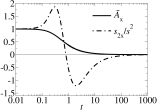
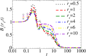
Figure 1: Left: Behavior of $\widetilde{A}_{\mathrm{x}}$ and $s_{\mathrm{2x}}/s^{2}\equiv\widetilde{B}_{\mathrm{x}}/\widetilde{A}_{\mathrm{x}}$ as functions of t. Right: Comparison of $\widetilde{B}_{\mathrm{c}}(r_{\mathrm{s}},t)$ reference data (symbols) and analytical fit (curves) for selected $r_{\mathrm{s}}$ values.

A well-behaved X enhancement factor arises from imposition of the following constraints: [i] $F_{\mathrm{x}}(0)=1$ to recover the HEG limit at all T; [ii] recovery of the T-dependence of the GE2 in the small-$s$ limit $F_{\mathrm{x}}(s_{2\mathrm{x}})\approx 1+\nu_{\mathrm{x}}s_{2\mathrm{x}}$ with $\nu_{\mathrm{x}}$ a constant consistent with the $s^{2}$ coefficient in the T=0K limit GGA; [iii] local satisfaction of the zero-T Lieb-Oxford bound Lieb.Oxford.1981 by requiring $F_{\mathrm{x}}(s_{2\mathrm{x}})\leq F_{\mathrm{x,max}}=1.804$ (see PerdewBurkeErnzerhof96 ); [iv] smooth, non-negative behavior for all $s_{2\mathrm{x}}\in\,]-\infty,+\infty[$, to match the behavior of exact X at finite-T Greiner.Carrier.Goerling.FT-EXX .

A simple enhancement factor

$$F_{\mathrm{x}}(s_{2\mathrm{x}})=1+\frac{\nu_{\mathrm{x}}s_{2\mathrm{x}}}{1+\alpha|s_{2\mathrm{x}}|}\,,$$ (10)

with $\alpha=\nu_{\mathrm{x}}/(F_{\mathrm{x,max}}-1)$ satisfies all of those constraints. Additionally, (10) with suitably chosen constants recovers PBE X in the zero-T limit: $s_{2\mathrm{x}}\rightarrow s^{2}$ $\Rightarrow$ $\lim_{\mathrm{T}\rightarrow 0}F_{\mathrm{x}}(s_{2\mathrm{x}})=1+\nu_{\mathrm{x}}s^{2}/(1+\alpha s^{2})$. In the high-T limit, the density-gradient dependence of $s_{\mathrm{2x}}$ is suppressed by the decaying tail of the $\widetilde{B}_{\mathrm{x}}(t)/\widetilde{A}_{\mathrm{x}}(t)$ function (see Fig. 1), such that $\lim_{\mathrm{T}\rightarrow\infty}F_{\mathrm{x}}(s_{2\mathrm{x}})=1$. Constraint [i] thus is satisfied not only for the strictly homogeneous case ($s=0$), but also for non-uniform densities with any finite $s$ value. This property is inherited correctly by the finite-T GGA, Eq. (10), from the GE2, Eq. (5).

Finite-T GGA Correlation.Recall that C and X differ in that $\widetilde{B}_{\mathrm{c}}$ depends upon both $n$ and $t$. The Supplemental Material SuppMat gives details of the $\widetilde{B}_{\mathrm{c}}$ analytical fit developed in this work. It uses numerical results from Ref. Sjostrom.Daligault.2014A , static local field corrections Niklasson..Singwi.1975 ; Gupta.Singwi.1977 , and quantum Monte-Carlo data for the finite-T HEG BrownEtAl2013 . The right-hand panel of Fig. 1 shows the smooth T and $r_{\mathrm{s}}$ dependencies of $\widetilde{B}_{\mathrm{c}}$. It is everywhere positive, goes to unity in the zero-$t$ limit (by construction), and vanishes in the high-T limit (thereby guaranteeing the correct high-T limit for correlation). At and below $t\approx 0.2$, enforcement of total entropy positivity for physical systems necessitated that the $\widetilde{B}_{\mathrm{c}}$ fit lie below the data SuppMat .

With $\widetilde{B}_{\mathrm{c}}$ in hand, the fact that the C term in Eq. (2) is proportional to $n^{1/3}s^{2}\widetilde{B}_{\mathrm{c}}(r_{\mathrm{s}},t)\propto q^{2}\widetilde{B}_{\mathrm{c}}(r_{\mathrm{s}},t)$ (with $q(n,\nabla n)=|\nabla n|/2k_{\mathrm{s}}n$ the ground-state variable and $k_{\mathrm{s}}=2(3n/\pi)^{1/6}$) motivates definition of the T-dependent reduced density gradient for C as

$$q_{\mathrm{c}}(n,\nabla n,{\mathrm{T}})=q(n,\nabla n)\sqrt{\widetilde{B}_{\mathrm{c}}(r_{\mathrm{s}},t)}\,,$$ (11)

In terms of $q_{\mathrm{c}}$, the finite-T GGA C functional is determined by imposition of the following conditions. The functional must [v] provide the correct HEG limit both at zero- and at finite-T,i.e. reduce to the LDA C (free-) energy; [vi] reproduce the slowly varying regime correctly; for T$>0$ the correct T-dependence in that regime is given by $\widetilde{B}_{\mathrm{c}}$; [vii] satisfy known T=0K constraints for C (e.g. Ref. PerdewBurkeErnzerhof96 ); [viii] reduce to the LDA C free energy in the high-T limit for any $n$ with finite reduced gradient $q$ (in consequence of the finite-T gradient expansion).

The simplest approximation which satisfies all these constraints is based on a known zero-T GGA correlation functional (which satisfies [vii]). T-dependence is introduced by adapting the PBE form of C energy per particle (spin-unpolarized) to become

$$\!\!\!\!\!f_{\mathrm{c}}^{\mathrm{GGA}}(n,\nabla n,{\mathrm{T}})=f_{\mathrm{c}}^{\mathrm{LDA}}(n,{\mathrm{T}})+H\Big{(}f_{\mathrm{c}}^{\mathrm{LDA}},\zeta=0,q_{\mathrm{c}}\Big{)}\,,$$ (12)

where $f_{\mathrm{c}}^{\mathrm{LDA}}$ is the LDA correlation free-energy per particle, $\zeta$ is the spin polarization fraction, and $H$ is as defined in PBE PerdewBurkeErnzerhof96 , but with substitutions as shown. Details are in Ref. SuppMat . Thus the GGA correlation free-energy is ${\mathcal{F}}_{\mathrm{c}}^{\mathrm{GGA}}[n,\mathrm{T}]=\int nf_{\mathrm{c}}^{\mathrm{GGA}}(n,\nabla n,{\mathrm{T}})d\mathbf{r}$. In the rapidly varying case, $f_{\mathrm{c}}^{\mathrm{GGA}}$ vanishes due to a ground state PBE C functional property, $\lim_{q_{\mathrm{c}}\rightarrow\infty}H=-f_{\mathrm{c}}^{\mathrm{LDA}}$. In the slowly varying regime, $f_{\mathrm{c}}^{\mathrm{GGA}}$ recovers the second-order gradient expansion (see Refs. PerdewBurkeErnzerhof96 ; Wang.Perdew.1991 ) with T-dependence described by $\widetilde{B}_{\mathrm{c}}$. Together with the GE2 for X, that also provides the correct XC T-dependence defined by Eqs. (1)-(2).

Because $\widetilde{B}_{\mathrm{c}}$ vanishes in the high-T limit, requirement [viii] is satisfied (analogously with the X case) for all densities with finite values of the variable $q$. This follows from $\lim_{\mathrm{T}\rightarrow\infty}H\Big{(}f_{\mathrm{c}}^{\mathrm{LDA}},\zeta,q_{\mathrm{c}}\Big{)}=0$. Thus the GGA XC free-energy functional, ${\mathcal{F}}_{\mathrm{xc}}^{\mathrm{GGA}}[n,\mathrm{T}]\equiv{\mathcal{F}}_{\mathrm{x}}^{\mathrm{GGA}}[n,\mathrm{T}]+{\mathcal{F}}_{\mathrm{c}}^{\mathrm{GGA}}[n,\mathrm{T}]$, reduces in the high-T limit to the LDA XC free-energy and eventually vanishes,

$$\lim_{\mathrm{T}\rightarrow\infty}({\mathcal{F}}_{\mathrm{xc}}^{\mathrm{GGA}}[n,\mathrm{T}]-{\mathcal{F}}_{\mathrm{xc}}^{\mathrm{LDA}}[n,\mathrm{T}])=0\,,$$ (13)

for any density $n$ with finite reduced gradients $s$ and $q$.

We used PBE values, $\nu_{\mathrm{x}}=0.21951$ in Eq. (10), and $\beta_{\mathrm{c}}=0.066725$ in $H$, Eq. (12). (Remark: to avoid notational ambiguity, $\nu_{\mathrm{x}}$ and $\beta_{\mathrm{c}}$ are the constants denoted $\mu$ and $\beta$ in Ref. PerdewBurkeErnzerhof96 .) Thus the T=0K limit of our functional, ${\mathcal{F}}_{\mathrm{xc}}^{\mathrm{GGA}}[n,\mathrm{T}]$, is the ground-state PBE functional, with the minor difference that we use the corrected KSDT (corrKSDT) parametrization as a suitably accurate LDA XC free-energy expression KSDT ; corrKSDT . Note, however, that virtually any ground-state GGA XC functional can be extended systematically into an XC free energy functional by use of the framework presented above.

Exemplary WDM Applications An AIMD simulation which directly probes the accuracy of the new GGA functional (“KDT16”), is for deuterium at two material densities and T well into the WDM regime. Figure 2 compares KDT16 and PBE pressures $P$ relative to high-quality PIMC data Hu.Militzer..2011 (shown for intermediate and high T only due to low-T PIMC limitations FxcSignif ). PBE systematically over-estimates the pressure. The deviation is significant at T=62.5, 95.25 and 125kK for both material densities, then decreases as the non-interacting free-energy dominates in the high-T limit. In contrast, the KDT16 pressures are in excellent agreement with the PIMC values for the entire T-range, with relative deviations $\leq$ 3%.

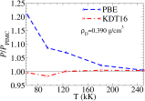
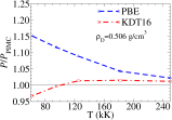
Figure 2: Ratios of Deuterium electronic pressure versus T for the free-energy GGA (“KDT16”) and ground-state PBE XC functionals, to PIMC reference results. AIMD PAW simulations, $\Gamma$-point only, for 64 atoms (4500 steps, T$\leq 125$kK) and 32 atoms (4500 steps, T$\geq 125$kK); timestep 25-50 asec.

This is a crucial finding two ways. First is that PIMC codes are not widely available, they are expensive to run, and PIMC itself is limited as to how far down in T it can go. Second is that hydrodynamic simulations of cryogenic inertial confinement implosions using the PIMC equation of state (EOS) tables found significant differences with respect to simulations based on the SESAME tables HuMilitzerGoncharovSkupsky2010 . The percentage shifts of pressures from KDT16 versus PBE are comparable to the PIMC to SESAME $P$ shifts, so using KDT16 instead of PBE should have similar impact on hydrodynamic simulations. Note consistency with the sensitivity of the deuterium principal Hugoniot to ground-state XC functional details KnudsonDesjarlais17 .

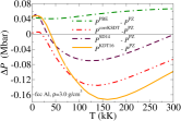
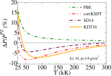
Figure 3: Left: Electronic pressure differences $\Delta P({\mathrm{T}})$ for the new KDT16 GGA, SD14 mixed LDA-GGA, corrKSDT LDA, and ground-state PBE XC functionals, all referenced to PZ ground-state LDA values. Fcc Al, 3.0 g/cm³. Right: Relative differences.

To isolate static lattice effects, the equation of state for fcc Al over a wide T range, $0\leq{\mathrm{T}}\leq 300$kK, at slightly compressed material density $\rho=3.0$ g/cm³ (as used in LCLS experiments LCLS.2015 ) was calculated from three thermal XC functionals, the new KDT16, SD14, corrKSDT, and two ground-state functionals (PZ PZ81 LDA and PBE GGA). Because LDA is widely viewed as good for metals, PZ is used as the reference. Calculations were done with a locally modified version of Quantum-Espresso QE ; ProfessQE . For the PZ and corrKSDT functionals we used a PAW data set built with PZ XC. For KDT16, SD14, and PBE we used the PBE PAW data set. All the calculations were otherwise self-consistent.

The resulting pressure differences shown in Fig. 3 distinguish XC inhomogeneity effects (see $(P^{\mathrm{PBE}}-P^{\mathrm{PZ}})$), thermal XC effects at the LDA level of refinement (see $(P^{\mathrm{corrKSDT}}-P^{\mathrm{PZ}})$), and the combined XC effects at the GGA refinement level in ($P^{\mathrm{KDT16}}-P^{\mathrm{PZ}}$). The new KDT16 functional interpolates smoothly between the PBE values at low-T and the corrKSDT (LDA) values at high-T (not fully shown). Pressure differences from both KDT16 and from corrKSDT have their maximum magnitude at intermediate-T, then decrease. Crucially, the ground state approximation, i.e. ${\mathcal{F}}_{\mathrm{xc}}^{\mathrm{GGA}}[n,\mathrm{T}]\approx E_{\mathrm{xc}}^{\mathrm{GGA}}[n]$ systematically overestimates the pressure by as much as $\approx$10% at T between $\approx 40$ and $100$kK. The pressures from all proper functionals eventually go to a common high-T limit as the XC contribution becomes negligible compared to the non-interacting free-energy. However, the behavior en route to that limit is qualitatively different for a free-energy GGA versus a ground-state functional. Note that SD14 pressures start to deviate significantly from the values given by KDT16 at ${\mathrm{T}}=50$kK ($t\approx 0.27$), roughly the beginning of the WDM regime.

Most importantly, the $\Delta P({\mathrm{T}})$ behavior of all three T-dependent XC functionals differs qualitatively from that from PBE. $\Delta P({\mathrm{T}})$ for PBE is uniformly positive, whereas $\Delta P(T)$ is negative for each of the explicitly T-dependent functionals above some relatively small T. Almost surely, therefore, the T-dependence from PBE is wrong. This qualitative distinction in the calculated EOS will have direct consequences for material predictions. An example is calibration of effective potential approaches. Ref. WunschVorbergerGericke2009 compared the Al ion-pair distribution from such a scheme with PBE AIMD results for T=1.1 eV, $\rho=$ 3.4 g/cm³ and deemed the agreement satisfactory. A similar comparison for the so-called ion feature recently is in Ref. Harbour..Lewis2016 . For T=10 eV and $\rho$ = 8.1 g/cm³, their “NPA” model with T_ion = 1.8 eV compares much more favorably with the experimental peak height than the AIMD result with PBE XC. Indeed, Rüter and Redmer RuterRedmer2014 had done an AIMD PBE static structure factor calculation at T=1,023 K ($\approx$ 0.1 eV), $\rho$ = 2.35 g/cm³ that agreed well with experiment for Al. But at T = 10 eV, $\rho$= 8.1 g/cm³ their AIMD-PBE calculation seriously underestimated the experimental ion-feature peak height. They attributed this discrepancy to omission of core electron effects but had no way to assess EOS effects which we have shown here to be substantial.

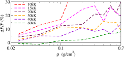
Figure 4: Relative difference in Al total pressure along six isotherms (10, 15, 20, 30, 40, 60 kK) for KDT16 and PBE XC functionals plotted as $(P^{\mathrm{PBE}}-P^{\mathrm{KDT16}})/P^{\mathrm{KDT16}}\times 100$.

Given the importance of EOS shifts, our final example is low density Al; its measured electrical conductivity exhibits pronounced system density dependence DeSilva.Katsouros.1998 . Fig. 4 shows that the low-density Al total pressure is strongly affected by use of the fully gradient-dependent and T-dependent XC functional. Shifts relative to it caused by the ground-state PBE approximation range as high as $\approx$50% (T=10kK) down to 5% (T=60kK). Clearly there is no simple rule-of-thumb correction for the ground-state functional data. Nor, on fundamental grounds, is there any reason to assume that it is the better of the two functionals. (Remark: Figure S2 in the Supplemental Material shows the ineffectiveness in identifying errors via direct comparison of KDT16 and PBE results.)

Implications and Summary. The non-empirical KDT16 GGA XC free-energy functional is more systematically constructed and general than the only previous attempt at a finite-T GGA Sjostrom.Daligault.2014A . KDT16 treats both density inhomogeneity and T-dependence effects yet distinguishes them clearly. Three rather different example calculations show its accuracy and value.They also confirm that ground-state GGA functionals are not routinely reliable as free energy functionals FxcSignif ; DanelKazandjianPrion2016 ; Schoof..Bonitz.PRL2015 ; Dornheim..Bonitz.PRL2016 .

The new ${\mathcal{F}}_{\mathrm{xc}}^{\mathrm{GGA}}$ has no empirical parameters. As with ground-state functionals, it involves design choice PerdewBurkeErnzerhof96 ; PBEsol ; PBEmol for the gradient-expansion coefficient for X ($\nu_{\mathrm{x}}$) and the related C parameter ($\beta_{\mathrm{c}}$). Yet the underlying procedure is general. Analysis of the XC gradient expansion leads to appropriate T-dependent variables for X and C. Together with the new $\widetilde{B}_{\mathrm{c}}(r_{\mathrm{s}},t)$ parametrization and the LDA free-energy parametrization KSDT ; corrKSDT , one has the basis for GGA XC free-energy functional development. Virtually any ground-state GGA XC functional thus can be extended systematically into an XC free energy functional by use of the T-dependent variables Eqs. (7), (11) within this framework.

- (1) B.B.L. Witte, L.B. Fletcher, E. Galtier, E. Gamboa, H.J. Lee, U. Zastrau, R. Redmer, S.H. Glenzer, and P. Sperling, Phys. Rev. Lett. 118, 225001 (2017).
- (2) L.X. Benedict, M.P. Surh, L.G. Stanton, C.R. Scullard, A.A. Correa, J.I. Castor, F.R. Graziani, L.A. Collins, O. Čertík, J.D. Kress, and M.S. Murillo, Phys. Rev. E 95, 043202 (2017).
- (3) M.P. Desjarlais, C.R. Scullard, L.X. Benedict, H.D. Whitley, and R. Redmer, Phys. Rev. E 95, 033203 (2017).
- (4) T. Dornheim, S. Groth, F.D. Malone, T. Schoof, T. Sjostrom, W.M.C. Foulkes, and M. Bonitz, Phys. Plas. 24, 056303 (2017).
- (5) K.P. Driver and B. Militzer, Phys. Rev. E 95, 043205 (2017).
- (6) K.P. Driver, F. Soubiran, S. Zhang and B. Militzer, High En. Dens. Phys. 23, 81 (2017).
- (7) S. Feldman, G. Dyer, D. Kuk, and T. Ditmire, Phys. Rev. E 95, 031201(R) (2017).
- (8) L. Harbour, M.W.C. Dharma-wardana, D.D. Klug, and L.J. Lewis, Phys. Rev. E 95, 043201 (2017).
- (9) S.X. Hu, R. Gao, Y. Ding, L.A. Collins, and J.D. Kress, Phys. Rev. E 95, 043210 (2017).
- (10) M.D. Knudson and M.P. Desjarlais, Phys. Rev. Lett. 118, 035501 (2017).
- (11) X. Vaisseau, A. Morace, M. Touati, M. Nakatsutsumi, S.D. Baton, S. Hulin, P. Nicolaï, R. Nuter, D. Batani, F.N. Beg, J. Breil, R. Fedosejevs, J.-L. Feugeas, P. Forestier-Colleoni, C. Fourment, S. Fujioka, L. Giuffrida, S. Kerr, H.S. McLean, H. Sawada, V.T. Tikhonchuk, and J.J. Santos, Phys. Rev. Lett. 118, 205001 (2017).
- (12) B.B.L. Witte, M. Shihab, S.H. Glenzer, and R. Redmer, Phys. Rev. B 95, 144105 (2017).
- (13) S. Zhang, K. Driver, F. Soubiran, and B. Militzer, J. Chem. Phys. 146, 074505 (2017).
- (14) K. Burke, J.C. Smith, P.E. Grabowski, and A. Pribram-Jones, Phys. Rev. B 93, 195132 (2016).
- (15) J.-F. Danel, L. Kazandjian, and R. Piron, Phys. Rev. E 93, 043210 (2016).
- (16) M.D. Knudson, M.P. Desjarlais, A. Becker, R.W. Lemke, K.R. Cochrane, M.E. Savage, D.E. Bliss, T.R. Mattsson, R. Redmer, Science, 348, 1455 (2015).
- (17) A. Becker, W. Lorenzen, J.J. Fortney, N. Nettelmann, M. Schöttler, and R. Redmer, Astrophys. J. Supp. 215, 21 (2014).
- (18) A. Benuzzi-Mounaix et al., Phys. Scr. T161, 014060 (2014) doi:10.1088/0031-8949/2014/T161/014060 .
- (19) H.R. Rüter and R. Redmer, Phys. Rev. Lett. 112, 145007 (2014).
- (20) Frontiers and Challenges in Warm Dense Matter, F. Graziani, M.P. Desjarlais, R. Redmer, and S.B. Trickey eds. (Springer Verlag, Heidelberg, 2014).
- (21) “Experimental Evidence for a Phase Transition in Magnesium Oxide at Exoplanet Pressures”, F. Coppari, R.F. Smith, J.H. Eggert, J. Wang, J.R. Rygg, A. Lazicki, J.A. Hawreliak, G.W. Collins, and T.S. Duffy, Nature Geosci. 6, 926–929 (2013)
- (22) H.F. Wilson and B. Militzer, Phys. Rev. Lett. 108, 111101 (2012).
- (23) R.P. Drake, Phys. Today 63, 28-33 (2010) and refs. therein.
- (24) M.D. Knudson and M.P. Desjarlais, Phys. Rev. Lett. 103, 225501 (2009).
- (25) Basic Research Needs for High Energy Density Laboratory Physics (Report of the Workshop on Research Needs, Nov. 2009). U.S. Department of Energy, Office of Science and National Nuclear Security Administration (2010); see Chapter 6 and refs. therein.
- (26) L.B. Fletcher et al., Nat. Photonics 9, 274 (2015).
- (27) P. Sperling et al., Phys. Rev. Lett. 115, 115001 (2015).
- (28) O. Ciricosta et al., Nat. Commun. 7, 11713 (2016).
- (29) D.J. Hoarty et al., Phys. Rev. Lett. 110, 265003 (2013).
- (30) R. Nora et al., Phys. Rev. Lett. 114, 045001 (2015).
- (31) M.C. Gregor et al., Phys. Rev. B 95, 144114 (2017).
- (32) A. Schönlen et al., Euro. Phys. Lett. 114, 45002 (2016).
- (33) N.D. Mermin, Phys. Rev. 137, A1441 (1965).
- (34) M.V. Stoitsov and I.Zh. Petkov, Annals Phys. 185, 121 (1988).
- (35) V.V. Karasiev, D. Chakraborty, J.W. Dufty, F.E. Harris, K. Runge, and S.B. Trickey, in IPAMreview p. 61.
- (36) S.M. Vinko, O. Ciricosta, and J.S. Wark, Nat. Commun. 5, 3533 (2014).
- (37) S.X. Hu, Phys. Rev. Lett. 119, 065001 (2017).
- (38) R.N. Barnett and U. Landman, Phys. Rev. B 48, 2081 (1993).
- (39) D. Marx and J. Hutter in Modern Methods and Algorithms of Quantum Chemistry, J. Grotendorst ed., John von Neumann Institute for Computing, (Jülich, NIC Series, Vol. 1, 2000) 301 and refs. therein.
- (40) J.S. Tse, Annu. Rev. Phys. Chem. 53, 249 (2002).
- (41) Ab Initio Molecular Dynamics: Basic Theory and Advanced Methods, D. Marx and J. Hutter, (Cambridge University Press, Cambridge, 2009) and refs. therein.
- (42) V.V. Karasiev, T. Sjostrom, J. Dufty, and S.B. Trickey, Phys. Rev. Lett. 112, 076403 (2014).
- (43) See Supplemental Material SuppMat for KSDT parameters corrected for a recently discovered small error in the original. Here we use corrected KSDT (corrKSDT) as the finite-T LDA XC; differences with original KSDT are almost nil. Use of the recent Groth et al. LDA, Phys. Rev. Lett. 119, 115101 (2017), would change nothing; see Supp. Mat.
- (44) V.V. Karasiev, L. Calderín, and S.B. Trickey, Phys. Rev. E 93, 063207 (2016).
- (45) V.V. Karasiev, T. Sjostrom, and S.B. Trickey, Phys. Rev. E 86, 056704 (2012).
- (46) T. Sjostrom, F.E. Harris, and S.B. Trickey, Phys. Rev. B 85, 045125 (2012).
- (47) F. Perrot and M.W.C. Dharma-wardana, Phys. Rev. A 30, 2619 (1984).
- (48) F. Perrot and M.W.C. Dharma-wardana, Phys. Rev. B 62, 16536 (2000); F. Perrot and M.W.C. Dharma-wardana, Phys. Rev. B 67, 079901(E) (2003).
- (49) T. Sjostrom and J. Daligault, Phys. Rev. B 90, 155109 (2014).
- (50) V.V. Karasiev, T. Sjostrom, and S.B. Trickey, Phys. Rev. B 86, 115101 (2012).
- (51) J.P. Perdew, K. Burke, and M. Ernzerhof, Phys. Rev. Lett. 77, 3865 (1996); erratum ibid. 78, 1396 (1997).
- (52) J.C. Pacheco-Kato, J.M. del Campo, J.L. Gázquez, S.B. Trickey, and A. Vela, Chem. Phys. Lett. 651, 268 (2016).
- (53) P. Hohenberg and W. Kohn, Phys. Rev. 136, B864 (1964).
- (54) W. Kohn and L.J. Sham, Phys. Rev. 140, A1133 (1965).
- (55) E. Dunlap and D.J.W. Geldart, Can. J. Phys. 72, 1 (1994).
- (56) M.L. Glasser, D.J.W. Geldart, and E. Dunlap, Can. J. Phys. 72, 7 (1994).
- (57) E. Dunlap, and D.J.W. Geldart, Can. J. Phys. 72, 14 (1994).
- (58) D.J.W. Geldart, Top. Curr. Chem. 180, 31 (1996).
- (59) J.S. Blakemore, Sol. State Electr. 25, 1067 (1982).
- (60) J. Bartel, M. Brack, and M. Durand, Nucl. Phys. A445, 263 (1985).
- (61) Values , in Eq. (2) correspond, to the X free-energy Geldart.SSC.1994 and T=0K C energy of the non-polarized slowly-varying electron gas Wang.Perdew.1991 .
- (62) F. Perrot, Phys. Rev. A 20, 586 (1979).
- (63) D.J.W. Geldart, E. Dunlap, M.L. Glasser, and M.R.A. Shegelski, Solid State Commun. 88, 81 (1993).
- (64) Whether the coefficient in Eq. (5) is 8/81 or 10/81 as in Refs. FactorRefs is irrelevant. Here we must match the small behavior of the ground state GGA X functional chosen for the TK limit, i.e., PBE.
- (65) L. Kleinman and V. Sahni, Adv. Quantum Chem. 21, 201 (1990) and refs. therein; E. Engel and S.H. Vosko, Phys. Rev. B 42, 4940 (1990), erratum ibid. 44, 1446 (1991).
- (66) V.V. Karasiev, D. Chakraborty, and S.B. Trickey, Comput. Phys. Commun. 192, 114 (2015).
- (67) S. Pittalis, C.R. Proetto, A. Floris, A. Sanna, C. Bersier, K. Burke, and E.K.U. Gross, Phys. Rev. Lett. 107, 163001 (2011).
- (68) J.W. Dufty and S.B. Trickey, Mol. Phys. 114, 988 (2016).
- (69) E.H. Lieb, and S. Oxford, Int. J. Quantum Chem. 19, 427 (1981).
- (70) M. Greiner, P. Carrier, and A. Görling, Phys. Rev. B 81, 155119 (2010).
- (71) See Supplemental Material.
- (72) G. Niklasson, A. Sjölander, and K.S. Singwi, Phys. Rev. B 11, 113 (1975).
- (73) A.K. Gupta and K.S. Singwi, Phys. Rev. B 15, 1801 (1977).
- (74) E.W. Brown, B.K. Clark, J.L. DuBois, and D.M. Ceperley, Phys. Rev. Lett. 110, 146405 (2013).
- (75) Y. Wang and J.P. Perdew, Phys. Rev. B 43, 8911 (1991).
- (76) S.X. Hu, B. Militzer, V.N. Goncharov, and S. Skupsky, Phys. Rev. B 84 224109 (2011).
- (77) S.X. Hu, B. Militzer, V.N. Goncharov, and S. Skupsky Phys. Rev. Lett. 104, 235003 (2010).
- (78) J.P. Perdew, and A. Zunger, Phys. Rev. B 23, 5048 (1981).
- (79) P. Giannozzi et al., J. Phys.: Condens. Matter 21, 395502 (2009).
- (80) V.V. Karasiev, T. Sjostrom, and S.B. Trickey, Comput. Phys. Commun. 185, 3240 (2014).
- (81) K. Wünsch, J. Vorberger, and D.O. Gericke, Phys. Rev. E 79, 010201(R) (2009).
- (82) L. Harbour, M.W.C. Dharma-wardana, D.D. Klug, and L.J. Lewis Phys. Rev. E 94, 053211 (2016).
- (83) H.R. Rüter and R. Redmer, Phys. Rev. Lett. 112, 145007 (2014).
- (84) A.W. DeSilva and J.D. Katsouros, Phys. Rev. E 57, 5945 (1998).
- (85) T. Schoof, S. Groth, J. Vorberger, and M. Bonitz, Phys. Rev. Lett. 115, 130402 (2015).
- (86) T. Dornheim, S. Groth, T. Sjostrom, F.D. Malone, W.M.C. Foulkes, and M. Bonitz, Phys. Rev. Lett. 117, 156403 (2016).
- (87) J.P. Perdew, A. Ruzsinszky, G.I. Csonka, O.A. Vydrov, G.E. Scuseria, L.A. Constantin, X. Zhou, and K. Burke, Phys. Rev. Lett. 100, 136406 (2008).
- (88) J.M. del Campo, J.L. Gázquez, S.B. Trickey, and A. Vela, J. Chem. Phys. 136, 104108 (2012).