Linearly Convergent Randomized Iterative Methods
for Computing the Pseudoinverse

Abstract

We develop the first stochastic incremental method for calculating the Moore-Penrose pseudoinverse of a real matrix. By leveraging three alternative characterizations of pseudoinverse matrices, we design three methods for calculating the pseudoinverse: two general purpose methods and one specialized to symmetric matrices. The two general purpose methods are proven to converge linearly to the pseudoinverse of any given matrix. For calculating the pseudoinverse of full rank matrices we present two additional specialized methods which enjoy a faster convergence rate than the general purpose methods. We also indicate how to develop randomized methods for calculating approximate range space projections, a much needed tool in inexact Newton type methods or quadratic solvers when linear constraints are present. Finally, we present numerical experiments of our general purpose methods for calculating pseudoinverses and show that our methods greatly outperform the Newton-Schulz method on large dimensional matrices.

MSC classes: 15A09, 15B52, 15A24, 65F10, 65F08, 68W20, 65Y20, 65F20, 68Q25, 68W40, 90C20
ACM class: G.1.3

1 Introduction

Calculating the pseudoinverse matrix is a basic numerical linear algebra tool required throughout scientific computing; for example in neural networks [28], signal processing [26, 12] and image denoising [1]. Perhaps the most important application of approximate pseudoinverse matrices is in preconditioning; for instance, within the approximate inverse preconditioning techniques [21, 15, 8, 4].

Currently, the pseudoinverse matrix is calculated using either the singular value decomposition or, when the dimensions of the matrix are large, using a Newton-Schulz type method [2, 3, 24]. However, neither of these aforementioned methods were designed with big data problems in mind, and when applied to matrices from machine learning, signal processing and image analysis, these classical methods can fail due exceeding the cache memory or take too much time.

In this paper we develop new fast stochastic incremental methods for calculating the pseudoinverse, capable of calculating an approximate pseudoinverse of truly large dimensional matrices. The problem of determining the pseudoinverse from stochastic measurements also serves as a model problem for determining an approximation to a high dimensional object from a few low dimensional measurements.

The new stochastic methods we present are part of a growing class of “sketch-and-project” methods [16], which have successfully been used for solving linear systems [19, 18], the distributed average consensus problem [22, 18] and inverting matrices [20].

We also envision that the new methods presented here for calculating pseudoinverse matrices will lead to the development of new quasi-Newton methods, much like the development of new randomized methods for inverting matrices [20] has lead to the development of new stochastic quasi-Newton methods [17].

1.1 The Moore-Penrose Pseudoinverse

The pseudoinverse of a real rectangular matrix $A\in\mathbb{R}^{m\times n}$ was first defined as the unique matrix $A^{\dagger}\in\mathbb{R}^{n\times m}$ that satisfies four particular matrix equations [25, 23]. However, for our purposes it will be more convenient to recall a definition using the singular value decomposition (SVD). Let $A=U\Sigma V^{\top}$ be the SVD of $A$, where $U\in\mathbb{R}^{m\times m}$ and $V\in\mathbb{R}^{n\times n}$ are orthogonal matrices and $\Sigma\in\mathbb{R}^{m\times n}$ is a diagonal matrix. The pseudoinverse $A^{\dagger}\in\mathbb{R}^{n\times m}$ is defined as $A^{\dagger}=V\Sigma^{\dagger}U^{\top}$, where $\Sigma^{\dagger}$ is the diagonal matrix with $\Sigma^{\dagger}_{ii}=1/\Sigma_{ii}$ if $\Sigma_{ii}\neq 0$ and $\Sigma^{\dagger}_{ii}=0$ otherwise. This immediately gives rise to a method for calculating the pseudoinverse via the SVD decomposition which costs $O(m^{2}n)$ floating point operations. When $m$ and $n$ are both large, this can be exacerbating and also unnecessary if one only needs a rough approximation of the pseudoinverse. Therefore, in this work we take a different approach.

In particular, it turns out that the pseudoinverse can alternatively be defined as the least-Frobenius-norm solution to any one of the three equations given in Lemma 1.

Lemma 1

The pseudoinverse matrix $A^{\dagger}$ is the least-Frobenius-norm solution of any of the three equations:

$$(P1)\quad AXA=A,\qquad(P2)\quad A^{\top}=XAA^{\top},\qquad\text{and}\qquad(P3)\quad A^{\top}=A^{\top}AX.$$

In Sections 2 and 3 we prove this statement for $(P1)$ and $(P2)$, and $(P3),$ respectively.

We use these three variational characterizations of the pseudoinverse given in Lemma 1 to design three different stochastic iterative methods for calculating the pseudoinverse. Based on (P2) and (P3), we propose two methods for calculating the pseudoinverse of any real matrix in Section 2. We exploit the symmetry in (P1) to propose a new randomized method for calculating the pseudoinverse of a symmetric matrix in Section 3.

In the next lemma we collect several basic properties of the pseudoinverse which we shall use often throughout the paper.

Lemma 2

Any matrix $A\in\mathbb{R}^{m\times n}$ and its pseudoinverse $A^{\dagger}\in\mathbb{R}^{n\times m}$ satisfy the following identities:

$$(A^{\dagger})^{\top} =(A^{\top})^{\dagger}\hskip 284.52756pt$$ (1)

$$A^{\top} =A^{\dagger}AA^{\top}$$ (2)

$$A^{\top} =A^{\top}AA^{\dagger}$$ (3)

$$\mathbf{Null}\left(A^{\dagger}\right) =\mathbf{Null}\left(A^{\top}\right)$$ (4)

Note that in the identities above the pseudoinverse behaves like the inverse would, were it to exist. Because of (1), we will use $A^{\dagger\top}$ to denote $(A^{\dagger})^{\top}$ or $(A^{\top})^{\dagger}$. Lemma 2 is a direct consequence of the definition of the pseudoinverse; see [25, 23] for a proof based on the classical definition and [11] for a proof based on a definition of the pseudoinverse through projections (all of which are equivalent approaches).

1.2 Notation

We denote the Frobenius inner product and norm by

$$\left<X,Y\right>\overset{\text{def}}{=}\mathbf{Tr}\left(X^{\top}Y\right)\qquad\mbox{and}\qquad\lVert X\rVert=\sqrt{\mathbf{Tr}\left(X^{\top}X\right)},$$

where $X$ and $Y$ are any compatible real matrices and $\mathbf{Tr}\left(X\right)$ denotes the trace of $X$. Since the trace is invariant under cyclic permutations, for matrices $X,Y,Z$ and $W$ of appropriate dimension, we have

$$\left<X,YZW\right>=\mathbf{Tr}\left(X^{\top}YZW\right)=\mathbf{Tr}\left((WX^{\top}Y)Z\right)=\left<Y^{\top}XW^{\top},Z\right>.$$ (5)

By $\mathbf{Null}\left(A\right)$ and $\mathbf{Range}\left(A\right)$ we denote the null space and range space of $A$, respectively. For a positive semidefinite matrix $G$, let $\lambda_{\min}^{+}(G)$ denote the smallest nonzero eigenvalue of $G$.

2 Sketch-and-Project Methods Based on (P3) and (P2)

In view of property (P3) of Lemma 1, the pseudoinverse can be characterized as the solution to the constrained optimization problem

$$A^{\dagger}\overset{\text{def}}{=}\arg\min\frac{1}{2}\lVert X\rVert^{2},\quad\mbox{subject to}\quad A^{\top}=A^{\top}AX.$$ (6)

We shall prove in Theorem 3 that the above variational characterization has the following equivalent dual formulation

$$A^{\dagger}=\arg_{X}\min_{X,\Gamma}\frac{1}{2}\lVert X-A^{\dagger}\rVert^{2},\quad\mbox{subject to}\quad X=A^{\top}A\Gamma.$$ (7)

The dual formulation (7) appears to be rather impractical, since using (7) to calculate $A^{\dagger}$ requires projecting the unknown matrix $A^{\dagger}$ onto a particular affine matrix space. But duality reveals that (7) can be calculated by solving the primal formulation (6), which does not require knowing the pseudoinverse a priori. The dual formulation reveals that we should not search for $A^{\dagger}$ within the whole space $\mathbb{R}^{n\times m}$ but rather, the pseudoinverse is contained in the matrix space which forms the constraint in (7).

In the next section we build upon the characterization (6) to develop a new stochastic method for calculating the pseudoinverse.

2.1 The method

Starting from an iterate $X_{k}\in\mathbb{R}^{n\times m}$, we calculate the next iterate $X_{k+1}\in\mathbb{R}^{n\times m}$ by drawing a random matrix $S\in\mathbb{R}^{m\times\tau}$ from a fixed distribution $\mathcal{D}$ (we do not pose any restrictions on $\tau$) and projecting $X_{k}$ onto the sketch of (P3):

$$X_{k+1}\overset{\text{def}}{=}\arg\min\frac{1}{2}\lVert X-X_{k}\rVert^{2},\quad\mbox{subject to}\quad S^{\top}A^{\top}=S^{\top}A^{\top}AX.$$ (8)

The dual formulation of (8) is given by

$$X_{k+1}\overset{\text{def}}{=}\arg_{X}\min_{X,\Gamma}\frac{1}{2}\lVert X-A^{\dagger}\rVert^{2},\quad\mbox{subject to}\quad X=X_{k}+A^{\top}AS\Gamma.$$ (9)

The duality of these two formulations is established in the following theorem, along with an explicit solution to (8) that will be used to devise efficient implementations.

Theorem 3

If $X_{k}\in\mathbf{Range}\left(A^{\top}A\right)$ then solving (6) and (8) is equivalent to solving (7) and (9), respectively. Furthermore, the explicit solution to (8) is given by

$$\boxed{X_{k+1}=X_{k}-A^{\top}AS(S^{\top}A^{\top}AA^{\top}AS)^{\dagger}S^{\top}A^{\top}(AX_{k}-I)}.$$ (10)

Proof: We will first show, using Lagrangian duality, that (8) and (9) are equivalent. The Lagrangian of (8) is given by

$$L(X,\Gamma) = \frac{1}{2}\lVert X-X_{k}\rVert^{2}+\left<\Gamma,S^{\top}A^{\top}AX-S^{\top}A^{\top}\right>$$ (11)

$$= \frac{1}{2}\lVert X-X_{k}\rVert^{2}+\left<A^{\top}AS\Gamma,X\right>-\left<\Gamma,S^{\top}A^{\top}\right>.$$

Since (8) is a convex optimization problem, strong duality implies that

$$\eqref{eq:ATAXdual}\quad=\quad\max_{\Gamma}\min_{X}L(X,\Gamma)=\min_{X}\max_{\Gamma}L(X,\Gamma)=\eqref{eq:ATAX}.$$

Differentiating (11) in $X$ and setting to zero gives

$$X=X_{k}-A^{\top}AS\Gamma.$$ (12)

Since $X_{k}\in\mathbf{Range}\left(A^{\top}A\right)$, using the above we conclude that $X_{k+1}\in\mathbf{Range}\left(A^{\top}A\right)$. Left multiplying by $S^{\top}A^{\top}A$ and observing the constraint in (8) gives $S^{\top}A^{\top}=S^{\top}A^{\top}AX_{k}-S^{\top}A^{\top}AA^{\top}AS\Gamma.$ Thus,

$$\mathbf{Range}\left(\Gamma\right)\subset(S^{\top}A^{\top}AA^{\top}AS)^{\dagger}S^{\top}A^{\top}(AX_{k}-I)+\mathbf{Null}\left(S^{\top}A^{\top}AA^{\top}AS\right).$$ (13)

From Lemma 13 with $G=AA^{\top}$ and $W=AS$ we have that $\mathbf{Null}\left(S^{\top}A^{\top}AA^{\top}AS\right)=\mathbf{Null}\left(A^{\top}AS\right).$ Consequently, left multiplying (13) by $A^{\top}AS$ gives

$$A^{\top}AS\Gamma = A^{\top}AS(S^{\top}A^{\top}AA^{\top}AS)^{\dagger}S^{\top}A^{\top}(AX_{k}-I).$$ (14)

The above combined with (12) gives (10).

To derive the dual of (8), first substitute (12) into (11)

$$L(X,\Gamma) = \frac{1}{2}\lVert X-X_{k}\rVert^{2}-\left<X-X_{k},X\right>-\left<\Gamma,S^{\top}A^{\top}AA^{\dagger}\right>$$ (15)

$$= -\frac{1}{2}\lVert X-X_{k}\rVert^{2}-\left<X-X_{k},X_{k}\right>-\left<A^{\top}AS\Gamma,A^{\dagger}\right>$$

$$= -\frac{1}{2}\lVert X-X_{k}\rVert^{2}+\left<X-X_{k},A^{\dagger}-X_{k}\right>\pm\frac{1}{2}\lVert A^{\dagger}-X_{k}\rVert^{2}$$

$$= -\frac{1}{2}\lVert X-X_{k}-(A^{\dagger}-X_{k})\rVert^{2}+\frac{1}{2}\lVert A^{\dagger}-X_{k}\rVert^{2}.$$

Calculating the argument that maximizes the above, subject to the constraint (12), is equivalent to solving (9). Thus (8) and (9) are dual to one another and consequently equivalent.

Finally, to see that (7) is the dual of (6), note that by substituting $X_{k}=0$ and $S=I$ into (8) and (9) gives  (6) and (7), respectively. Furthermore, when $S=I$ in  (10) we have that

$$X_{k+1} \overset{\eqref{eq:SATAXsol}+\text{Lemma}~{}\ref{lem:pseudo}}{=} X_{k}-A^{\top}A(A^{\top}AA^{\top}A)^{\dagger}A^{\top}A(X_{k}-A^{\dagger})$$

$$\overset{P1}{=} X_{k}-(X_{k}-A^{\dagger})=A^{\dagger},$$

where in the last equality we used that $X_{k}-A^{\dagger}\in\mathbf{Range}\left(A^{\top}A\right)$. Consequently the pseudoinverse is indeed the solution to (6) and (7).       

The bottleneck in computing (10) is performing the matrix-matrix product $S^{\top}A$, which costs $O(\tau mn)$ arithmetic operations. Since we allow $\tau$ to be any positive integer, even $\tau=1$, the iterations (10) can be very cheap to compute. Furthermore, method (8) converges linearly (in $L2$) under very weak assumptions on the distribution $\cal D$, as we show in the next section.

2.2 Convergence

Since the iterates (10) are defined by a projection process, as we shall see, proving convergence is rather straightforward. Indeed, we will now prove that the iterates (10) converge in $L2$ to the pseudoinverse; that is, the expected norm of $X_{k}-A^{\dagger}$ converges to zero. Furthermore, we have a precise expression for the rate at which the iterates converge.

The proofs of convergence of all our methods follow the same machinery. We first start by proving an invariance property of the iterates; namely, that all the iterates reside in a particular affine matrix subspace. We then show that $X_{k}-A^{\dagger}$ converges to zero within the said matrix subspace.

Lemma 4

If $\;\mathbf{Range}\left(X_{0}\right)\subset\mathbf{Range}\left(A^{\top}A\right),$ then the iterates (10) are such that
$\mathbf{Range}\left(X_{k}-A^{\dagger}\right)\subset\mathbf{Range}\left(A^{\top}A\right)$ for all $k.$

Proof: Using induction and the constraint in (9) we have that $\mathbf{Range}\left(X_{k}\right)\subset\mathbf{Range}\left(A^{\top}A\right)$ for all $k.$ The result now follows from $\mathbf{Range}\left(A^{\dagger}\right)\subset\mathbf{Range}\left(A^{\top}A\right)$ as can be seen in (7).       

Theorem 5

Let $X_{0}\in\mathbb{R}^{n\times m}$ with $\mathbf{Range}\left(X_{0}\right)\subset\mathbf{Range}\left(A^{\top}A\right)$ and let $H_{S}\overset{\text{def}}{=}S(S^{\top}A^{\top}AA^{\top}AS)^{\dagger}S^{\top}.$ The expected iterates (10) evolve according to

$$\mathbf{E}\left[X_{k+1}-A^{\dagger}\right]=\mathbf{E}\left[I-A^{\top}AH_{S}A^{\top}A\right]\mathbf{E}\left[X_{k}-A^{\dagger}\right].$$ (16)

Furthermore, if $\mathbf{E}\left[H_{S}\right]$ is finite and positive definite then

$$\mathbf{E}\left[\lVert X_{k}-A^{\dagger}\rVert^{2}\right]\leq\rho^{k}\,\lVert X_{0}-A^{\dagger}\rVert^{2},$$ (17)

where

$$\rho=1-\lambda_{\min}^{+}\left(A^{\top}A\mathbf{E}\left[H_{S}\right]A^{\top}A\right).$$ (18)

Proof: Let $R_{k}\overset{\text{def}}{=}X_{k}-A^{\dagger}$ and $Z\overset{\text{def}}{=}A^{\top}AS(S^{\top}(A^{\top}A)^{2}S)^{\dagger}S^{\top}A^{\top}A=A^{\top}AH_{S}A^{\top}A.$ Subtracting $A^{\dagger}$ from both sides of (10) we have

$$R_{k+1}=(I-Z)R_{k}.$$ (19)

Taking expectation conditioned on $R_{k}$ gives $\mathbf{E}\left[R_{k+1}\,|\,R_{k}\right]=(I-\mathbf{E}\left[Z\right])R_{k}.$ Taking expectation again gives (16). Using the properties of pseudoinverse, it is easy to show that $Z$ is a projection matrix and thus $I-Z$ is also a projection matrix. Taking norm squared and then expectation conditioned on $R_{k}$ in (19) gives

$$\mathbf{E}\left[\lVert R_{k+1}\rVert^{2}\,|\,R_{k}\right] = \mathbf{E}\left[\left<(I-Z)R_{k},(I-Z)R_{k}\right>\,|\,R_{k}\right]$$ (20)

$$\overset{(I-Z)\text{ is a proj.}}{=} \mathbf{E}\left[\left<(I-Z)R_{k},R_{k}\right>\,|\,R_{k}\right]$$

$$= \lVert R_{k}\rVert^{2}-\left<\mathbf{E}\left[Z\right]R_{k},R_{k}\right>.$$

From Lemma 4 we have that there exists $W_{k}$ such that $R_{k}=A^{\top}AW_{k}.$ Therefore,

$$\left<\mathbf{E}\left[Z\right]R_{k},R_{k}\right> \overset{\text{Lemma~{}\ref{lem:invariant}}}{=} \left<A^{\top}A\mathbf{E}\left[Z\right]A^{\top}AW_{k},W_{k}\right>$$ (21)

$$= \left<(A^{\top}A)(A^{\top}A)H_{S}(A^{\top}A)(A^{\top}A)W_{k},W_{k}\right>$$

$$\overset{\text{Lemma~{}\ref{lem:WGWtight} }}{\geq} \lambda_{\min}^{+}\left(A^{\top}AH_{S}A^{\top}A\right)\left<(A^{\top}A)W_{k},(A^{\top}A)W_{k}\right>$$

$$= \lambda_{\min}^{+}\left(A^{\top}AH_{S}A^{\top}A\right)\lVert R_{k}\rVert^{2}=(1-\rho)\,\lVert R_{k}\rVert^{2}.$$

Taking expectation in (20) we have

$$\mathbf{E}\left[\lVert R_{k+1}\rVert^{2}\right]=\mathbf{E}\left[\lVert R_{k}\rVert^{2}\right]-\mathbf{E}\left[\left<\mathbf{E}\left[Z\right]R_{k},R_{k}\right>\right]\overset{\eqref{eq:SATAtheo2}}{\leq}\rho\,\mathbf{E}\left[\lVert R_{k}\rVert^{2}\right].$$

It remains now to unroll the above recurrence to arrive at (17).       

With a precise expression for the convergence rate (18) opens up the possibility of tuning the distribution of $S$ so that the resulting has a faster convergence. Next we give an instantiation of the method (10) and indicate how one can choose the distribution of $S$ to accelerate the method. We refer to methods based on (10) as the SATAX methods, inspired on the constraint in (8) whose right hand side almost spells out SATAX. Later in Section 5 we perform experiments on variants of the SATAX method.

2.3 Discrete examples

Though our framework and Theorem 3 allows for $\mathcal{D}$ to be a continuous distribution, for illustration purposes here we focus our attention on developing examples where $\mathcal{D}$ is a discrete distribution.

For any discrete distribution $\mathcal{D}$ the random matrix $S\sim\mathcal{D}$ will have a finite number of possible outcomes. Fix $r$ as the number of outcomes and let $\tau\in\mathbb{N}$ and $S=S_{i}\in\mathbb{R}^{m\times\tau}$ with probability $p_{i}>0$ for $i=1,\ldots,r$. Let $\mathbb{S}\overset{\text{def}}{=}[S_{1},\ldots,S_{r}]\in\mathbb{R}^{m\times r\tau}$. If

$$p_{i}=\frac{\mathbf{Tr}\left(S_{i}^{\top}(A^{\top}A)^{2}S_{i}\right)}{\mathbf{Tr}\left(\mathbb{S}^{\top}(A^{\top}A)^{2}\mathbb{S}\right)},$$

then by Lemma 17 with $G=A^{\top}A$ as proven in the Appendix, the rate of convergence in Theorem 3 is given by

$$\rho=1-\lambda_{\min}^{+}(\mathbf{E}\left[Z\right])\leq 1-\frac{\lambda_{\min}^{+}(\mathbb{S}^{\top}(A^{\top}A)^{2}\mathbb{S})}{\mathbf{Tr}\left(\mathbb{S}^{\top}(A^{\top}A)^{2}\mathbb{S}\right)}.$$ (22)

The number $\left.\lambda_{\min}^{+}(\mathbb{S}^{\top}(A^{\top}A)^{2}\mathbb{S})\right/\mathbf{Tr}\left(\mathbb{S}^{\top}(A^{\top}A)^{2}\mathbb{S}\right)$ is known as the scaled condition number of $\mathbb{S}^{\top}(A^{\top}A)^{2}\mathbb{S}$ and it is the same condition number on which the rate of convergence of the randomized Kaczmarz method depends [27]. This rate (22) suggests that we should choose $\mathbb{S}$ so that $\mathbb{S}^{\top}(A^{\top}A)^{2}\mathbb{S}$ has a concentrated spectrum and consequently, the scaled condition number is minimized. Ideally, we would want $\mathbb{S}=(A^{\top}A)^{\dagger},$ but this is not possible in practice, though it does inspire the following heuristic choice. If we choose $r$ so that $r\tau=n$, then we can set $\mathbb{S}=X_{k}X_{k}^{\top},$ and consequently $X_{k}\rightarrow A^{\dagger}$ we have that $\mathbb{S}\rightarrow A^{\dagger}A^{\dagger\top}=(A^{\top}A)^{\dagger}.$ Though through experiments we have identified that choosing the sketch matrix so that $\mathbb{S}=X_{k}$ resulted in the best performance. This observation, together with other empirical observations, has lead us to suggest two alternative sketching strategies:

Uniform $\tau$–batch sampling:

We say $S$ is a uniform $\tau$–batch sampling if $\mathbf{P}(S=I_{:C})=\left.1\right/\binom{n}{|C|}$ where $C\in\{1,\ldots,n\}$ is a random subset with $|C|=\tau$ chosen uniformly at random and $I_{:C}$ denotes the column concatenation of the columns of the identity matrix indexed by $C.$

Adaptive sketching:

Fix the iteration count $k$ and consider the current iterate $X_{k}$. We say that $S$ is an adaptive sketching if $\mathbf{P}(S=X_{k}I_{:C})$ where $I_{:C}$ is a uniform $\tau$–batch sampling.

When using a uniform $\tau$–batch sampling together with the SATAX method, we refer to the resulting method as the SATAX_uni. We use SATAX_ada when referring to the method that uses the adaptive sketching. We benchmark both these methods later in Section 5.

2.4 A sketch-and-project method based on (P2)

Yet another characterization of the pseudoinverse is given by the solution to the constrained optimization problem based on property (P2):

$$A^{\dagger}\overset{\text{def}}{=}\arg\min\frac{1}{2}\lVert X\rVert^{2},\quad\mbox{subject to}\quad A^{\top}=XAA^{\top}.$$ (23)

which has the following equivalent dual formulation

$$A^{\dagger}\overset{\text{def}}{=}\arg_{X}\min_{X,\Gamma}\frac{1}{2}\lVert X-A^{\dagger}\rVert^{2},\quad\mbox{subject to}\quad X=\Gamma^{\top}AA^{\top}.$$ (24)

Transposing the constraint in (23) gives $A=AA^{\top}X^{\top}.$ Since the Frobenius norm is invariant to transposing the argument, we have that by setting $Y=X^{\top}$ in (23) we get

$$A^{\dagger\top}\overset{\text{def}}{=}\arg\min\frac{1}{2}\lVert Y\rVert^{2},\quad\mbox{subject to}\quad A=AA^{\top}Y.$$ (25)

It is now clear to see that (25) is equivalent to (6) where each occurrence of $A$ has been swapped for $A^{\top}.$ Because of this simple mapping from (25) to (6) we refrain from developing methods based on (25) (even though these methods are different).

3 A Sketch-and-Project Method Based on (P1)

Now we turn out attention to designing a method based on (P1). In contrast with the development in the previous section, here we make explicit use of the symmetry present in (P1). In particular, we introduce a novel sketching technique which we call symmetric sketch. As we shall see, if $A$ is symmetric, our method (30) maintains the symmetry of iterates if started from a symmetric matrix $X_{0}$. Throughout this section we assume that $A\in\mathbb{R}^{n\times n}$ is a symmetric matrix.

The final variational characterization of the pseudoinverse from Lemma 1, based on (P1), is

$$A^{\dagger}=\arg\min\frac{1}{2}\lVert X\rVert^{2},\quad\mbox{subject to}\quad AXA=A.$$ (26)

As before, we have the following equivalent dual formulation

$$A^{\dagger}=\arg_{X}\min_{\Gamma,X}\frac{1}{2}\lVert A^{\dagger}-X\rVert^{2}\quad\mbox{subject to}\quad X=A\Gamma A.$$ (27)

In Section 3.1 we describe our method. In Theorem 6 we prove that these two formulations are equivalent and also show that the iterates of our method are symmetric. This is in contrast with techniques such as the block BFGS update and other methods designed for calculating the inverse of a matrix in [20], where symmetry has to be imposed on the iterates through an explicit constraint.

Calculating approximations of the pseudoinverse of a symmetric matrix is particularly relevant when designing variable metric methods in optimization, where one wishes to maintain an approximate of the (pseudo)inverse of the Hessian matrix. In contrast to the symmetric methods for calculating the inverse presented in [20], which can be readily interpreted as extensions of known quasi-Newton methods, the method presented in this section appears not to be related to any Broyden quasi-Newton method [5], nor the SR1 update. This naturally leads to the question: how would a quasi-Newton method based on (30) fair? We leave this question to future research.

3.1 The method

Similarly to the methods developed in Section 2, we define an iterative method by projecting onto a sketch of (26). In this case, however, we use the symmetric sketch. Specifically, we calculate the next iterate $X_{k+1}$ via

$$X_{k+1}\overset{\text{def}}{=}\arg\min\frac{1}{2}\lVert X-X_{k}\rVert^{2},\quad\mbox{subject to}\quad S^{\top}AXAS=S^{\top}AS,$$ (28)

where $S\in\mathbb{R}^{m\times\tau}$ is drawn from $\mathcal{D}$. The dual formulation is given by

$$X_{k+1}=\arg_{X}\min_{\Gamma,X}\frac{1}{2}\lVert X-A^{\dagger}\rVert^{2}\quad\mbox{subject to}\quad X=X_{k}+AS\Gamma S^{\top}A.$$ (29)

This symmetric sketch makes its debut in this work, since it has not been used in any of the previous works developing sketch-and-project sketching methods [19, 18, 20].

Theorem 6

Solving (26) and (28) is equivalent to solving (27) and (29), respectively. Furthermore, the explicit solution to (28) is

$$\boxed{X_{k+1}=X_{k}+AS(S^{\top}A^{2}S)^{\dagger}S^{\top}(A-AX_{k}A)S(S^{\top}A^{2}S)^{\dagger}S^{\top}A.}$$ (30)

Proof: Let

$$E\overset{\text{def}}{=}X-X_{k}\quad\mbox{and}\quad B\overset{\text{def}}{=}S^{\top}(A-AX_{k}A)S.$$ (31)

Using the above renaming we have that (28) is equivalent to solving

$$\min\frac{1}{2}\lVert E\rVert^{2},\quad\mbox{subject to}\quad S^{\top}AEAS=B.$$ (32)

The Lagrangian of (32) is given by

$$L(E,\Gamma) = \frac{1}{2}\lVert E\rVert^{2}+\left<\Gamma,S^{\top}AEAS-B\right>$$ (33)

$$\overset{\eqref{eq:traceperm}}{=} \frac{1}{2}\lVert E\rVert^{2}+\left<AS\Gamma S^{\top}A,E\right>-\left<\Gamma,B\right>.$$

Differentiating in $E$ and setting the derivative to zero gives

$$E=-AS\Gamma S^{\top}A.$$ (34)

Left and right multiplying by $S^{\top}A$ and $AS$, respectively, and using the constraint in (32) gives

$$B=-(S^{\top}A^{2}S)\Gamma S^{\top}A^{2}S.$$ (35)

The equation (35) is equivalent to solving in $\Gamma$ the following system

$$(S^{\top}A^{2}S)Y = -B$$ (36)

$$(S^{\top}A^{2}S)\Gamma^{\top} = Y^{\top}.$$ (37)

The solution to (36) is given by any $Y$ such that

$$\mathbf{Range}\left(Y\right) \subset -(S^{\top}A^{2}S)^{\dagger}B+\mathbf{Null}\left(S^{\top}A^{2}S\right)$$ (38)

$$\overset{\text{Lemma~{}\ref{lem:09709s} }}{\subset} -(S^{\top}A^{2}S)^{\dagger}B+\mathbf{Null}\left(AS\right),$$

where we applied Lemma 13 with $G=I$ and $W=AS.$ The solution to (37) is given by any $\Gamma$ that satisfies

$$\mathbf{Range}\left(\Gamma^{\top}\right) \subset (S^{\top}A^{2}S)^{\dagger}Y^{\top}+\mathbf{Null}\left(S^{\top}A^{2}S\right)$$ (39)

$$\overset{\text{Lemma~{}\ref{lem:09709s} }}{\subset} (S^{\top}A^{2}S)^{\dagger}Y^{\top}+\mathbf{Null}\left(AS\right).$$

Transposing the above, substituting (38), left and right multiplying by $AS$ and $S^{\top}A$ respectively gives

$$\mathbf{Range}\left(AS\Gamma S^{\top}A\right) \subset AS\left(\mathbf{Null}\left(AS\right)-(S^{\top}A^{2}S)^{\dagger}B\right)(S^{\top}A^{2}S)^{\dagger}S^{\top}A$$

$$+AS\mathbf{Null}\left(AS\right)^{\top}S^{\top}A$$

$$= -AS(S^{\top}A^{2}S)^{\dagger}B(S^{\top}A^{2}S)^{\dagger}S^{\top}A,$$ (41)

where in the last step we used the fact that $(AS\mathbf{Null}\left(AS\right)^{\top}S^{\top}A)^{\top}=AS\mathbf{Null}\left(AS\right)S^{\top}A=0.$ Inserting (41) into (34) gives $E=AS(S^{\top}A^{2}S)^{\dagger}B(S^{\top}A^{2}S)^{\dagger}S^{\top}A.$ Substituting in the definition of $E$ and $B$ we have (30).

For the dual problem, using (34) and substituting (45) into (33) gives

$$L(E,\Gamma) = \frac{1}{2}\lVert E\rVert^{2}-\lVert E\rVert^{2}-\left<\Gamma,S^{\top}A(A^{\dagger}-X_{k})AS\right>$$

$$= -\frac{1}{2}\lVert E\rVert^{2}-\left<AS\Gamma S^{\top}A,X_{k}-A^{\dagger}\right>$$

$$\overset{\eqref{eq:LagSAXASEsoltemp}}{=} -\frac{1}{2}\lVert E\rVert^{2}+\left<E,X_{k}-A^{\dagger}\right>\pm\frac{1}{2}\lVert X_{k}-A^{\dagger}\rVert^{2}$$

$$= -\frac{1}{2}\lVert E-(A^{\dagger}-X_{k})\rVert^{2}+\frac{1}{2}\lVert X_{k}-A^{\dagger}\rVert^{2}.$$

Substituting $E=X-X_{k}$, maximizing in $\Gamma$ and minimizing in $X$ while observing the constraint (34), we arrive at (29).

Furthermore, substituting $X_{k}=0$ and $S=I$ in (28) and (29) gives (26) and (27), respectively, thus (26) and (27) are indeed equivalent dual formulations. Finally, substituting $X_{k}=0$ and $S=I$ in (30) and using properties P1 and P2, it is not hard to see that (30) is equal to $A^{\dagger},$ and thus (26) and (27) are indeed alternative characterizations of the pseudoinverse.       

One of the insights given by the dual formulation (29) is that the resulting method is monotonic, that is, the error $\lVert X_{k+1}-A^{\dagger}\rVert$ must be a decreasing sequence. Inspired on the constraint in (28), we refer to the class of methods defined by (28) as the SAXAS methods.

3.2 Convergence

Proving the convergence of the iterates (30) follows the same machinery as the convergence proof in Section 2.2. But different from Section 2.2 the resulting convergence rate $\rho$ may be equal to one $\rho=1$. We determine discrete distributions for $S$ such that $\rho<1$ in Section 3.3.

The first step of proving convergence is the following invariance result.

Lemma 7

Let $A,W\in\mathbb{R}^{n\times n}$ be symmetric matrices. If $X_{0}=AWA$ then for each $k\geq 0$ there exists matrix $Q_{k}\in\mathbb{R}^{n\times m}$ such that the iterates (30) satisfy $X_{k}-A^{\dagger}=AQ_{k}A.$

Proof: Using induction and the constraint in (29) we have that $X_{k+1}=AW_{k+1}A$ where $W_{k+1}=W_{k}+S\Gamma S^{\top}$. Furthermore, from the constraint in (29), we have that there exists $\Gamma$ such that $A^{\dagger}=A\Gamma A.$ Thus $X_{k+1}-A^{\dagger}=AQ_{k+1}A$ with $Q_{k+1}=W_{k+1}-\Gamma.$       

Theorem 8

Let $A,W\in\mathbb{R}^{n\times n}$ be symmetric matrices. If $X_{0}=AWA$ then the iterates (10) converge according to

$$\mathbf{E}\left[\lVert X_{k}-A^{\dagger}\rVert^{2}\right]\quad\leq\quad\rho^{k}\lVert X_{0}-A^{\dagger}\rVert^{2},$$ (42)

where

$$\rho\quad\overset{\text{def}}{=}\quad 1-\inf_{{\text{\scriptsize$\begin{array}[]{c}R=AQA,Q\in\mathbb{R}^{n\times n}\\ \lVert R\rVert^{2}=1\end{array}$ }}}\left<\mathbf{E}\left[ZRZ\right],R\right>,$$ (43)

and

$$Z\overset{\text{def}}{=}AS(S^{\top}A^{2}S)^{\dagger}S^{\top}A.$$ (44)

Proof: Let $R_{k}=X_{k}-A^{\dagger}$. Using

$$S^{\top}(A-AX_{k}A)S\overset{(P1)}{=}S^{\top}A(A^{\dagger}-X_{k})AS=S^{\top}AR_{k}AS,$$ (45)

and subtracting $A^{\dagger}$ from both sides of (30) gives

$$R_{k+1}=R_{k}-ZR_{k}Z.$$ (46)

Applying the properties of the pseudoinverse, it can be shown that $Z$ is a projection matrix, whence $Z^{2}=Z$. Taking norms and expectation conditioned on $R_{k}$ on both sides gives

$$\mathbf{E}\left[\lVert R_{k+1}\rVert^{2}\,|\,R_{k}\right] = \mathbf{E}\left[\left<R_{k}-ZR_{k}Z,R_{k}-ZR_{k}Z\right>\,|\,R_{k}\right]$$ (47)

$$\overset{Z\mbox{ \small is a proj.}}{=} \lVert R_{k}\rVert^{2}-\left<\mathbf{E}\left[ZR_{k}Z\right],R_{k}\right>.$$

By Lemma 7 and (47) we have that

$$\mathbf{E}\left[\lVert R_{k+1}\rVert^{2}\,|\,R_{k}\right] \overset{\eqref{eq:SAXASconv1}}{=} \lVert R_{k}\rVert^{2}-\left<\mathbf{E}\left[Z\frac{R_{k}}{\lVert R_{k}\rVert}Z\right],\frac{R_{k}}{\lVert R_{k}\rVert}\right>\lVert R_{k}\rVert^{2}.$$ (48)

$$\overset{\text{Lemma~{}\ref{lem:invariantAXA}}+\eqref{eq:rhoAXA}}{\leq} \rho\lVert R_{k}\rVert^{2}.$$

It remains to take expectations again, apply the tower property, and unroll the recurrence.       

The method described in (28) is particularly well suited to calculating an approximation to the pseudoinverse of symmetric matrices, since symmetry is preserved by the method.

Lemma 9 (Symmetry invariance)

If $X_{0}=X_{0}^{\top}$ and $A=A^{\top}$ then the iterates (30) are symmetric.

Proof: The constraint in (29) and induction shows that $X_{k}=X_{k}^{\top}$ holds for any $k.\hfill\nobreak\hskip 0.0pt\hskip 15.00002pt minus 5.0pt\nobreak\vrule height=7.5pt,width=5.0pt,depth=2.5pt$

3.3 The rate of convergence

It is not immediately obvious that (18) is a valid rate. That is, is it the case that $0\leq\rho\leq 1$? We give an affirmative answer to this in Lemma 11. Subsequently, in Lemma 12 we establish necessary and sufficient conditions on discrete distribution $\cal D$ to characterize when $\rho<1$. Consequently, under these conditions a linear convergence rate is guaranteed.

To establish the next results we make use of vectorization and the Kronecker product so that we can leverage on classic results in linear algebra. For convenience, we state several well known properties and equalities involving Kronecker products in the following lemma. But first, the Kronecker product of matrices $A\in\mathbb{R}^{m\times n}$ and $B\in\mathbb{R}^{p\times q}$ is defined as

$$(A\otimes B)_{p(r-1)+i,q(s-1)+j}=a_{rs}b_{ij}.$$ (49)

Let $\vec{A}\in\mathbb{R}^{nm}$ denote the vector obtained by stacking the columns of the matrix $A$ on top of one another.

Lemma 10 (Properties Kronecher products)

For matrices $A,B$ and $C$ of compatible dimensions we have that

1. $\overrightarrow{ABC}=(C^{\top}\otimes A)\vec{B},$

2. $(C\otimes B)^{\top}=C^{\top}\otimes B^{\top}.$

3. If $A$ and $B$ are symmetric positive semidefinite then $B\otimes A$ is symmetric positive semidefinite.

4. Since both vectorization and expectation are linear operators, if $Z$ is a random matrix then $\overrightarrow{\mathbf{E}\left[Z\right]}=\mathbf{E}\left[\vec{Z}\right].$

Lemma 11

The rate (43) satisfies $0\leq\rho\leq 1.$ Furthermore, if

$$\{R\,:\,\mathbf{E}\left[ZRZ\right]=0\}\subset\{R\,:\,ARA=0\},$$ (50)

then

$$\rho\leq 1-\lambda_{\min}^{+}(\mathbf{E}\left[Z\otimes Z\right])<1,$$ (51)

and the iterates (10) converge.

Proof: Since $Z$ is positive semidefinite we have that

$$\left<ZRZ,R\right>=\mathbf{Tr}\left(R^{\top}ZRZ\right)=\mathbf{Tr}\left(Z^{1/2}R^{\top}ZRZ^{1/2}\right)\geq 0.$$

Taking expectation in the above gives that $\rho\leq 1.$ Furthermore, since $Z$ is a projection matrix,

$$\left<ZRZ,R\right> = \mathbf{Tr}\left(R^{\top}ZRZ\right)$$

$$\leq \mathbf{Tr}\left(R^{\top}ZR\right)\underbrace{\lambda_{\max}(Z)}_{=1}$$

$$= \mathbf{Tr}\left(ZRR^{\top}\right)$$

$$\leq \mathbf{Tr}\left(RR^{\top}\right)\lambda_{\max}(Z)=\lVert R\rVert^{2}.$$

Dividing by $\lVert R\rVert^{2}$ and taking expectation over $Z$ gives

$$\frac{\left<\mathbf{E}\left[ZRZ\right],R\right>}{\lVert R\rVert^{2}}\leq 1.$$ (52)

Thus, for any $R\neq 0$, we have that

$$\rho\overset{\eqref{eq:rhoAXA}}{\geq}1-\frac{\left<\mathbf{E}\left[ZRZ\right],R\right>}{\lVert R\rVert^{2}}\overset{\eqref{eq:adj9823r}}{\geq}0,$$

which concludes the proof that $0\leq\rho\leq 1.$

After vectorizing and using item 1 of Lemma 10, the condition (50) is equivalent to

$$\{\vec{R}\,:\,\mathbf{E}\left[Z\otimes Z\right]\vec{R}=0\}=\mathbf{Null}\left(\mathbf{E}\left[Z\otimes Z\right]\right)\overset{\eqref{eq:AXArhonot0}}{\subset}\{\vec{R}\,:\,(A\otimes A)\vec{R}=0\}=\mathbf{Null}\left(A\otimes A\right).$$ (53)

Since $Z$ is symmetric positive semidefinite, item 3 of Lemma 10 states that the matrix $Z\otimes Z$, and consequently $\mathbf{E}\left[Z\otimes Z\right]$, are symmetric positive semidefinite. Thus taking orthogonal complements in (53) we have

$$\mathbf{Range}\left(A\otimes A\right)\subset\mathbf{Range}\left(\mathbf{E}\left[Z\otimes Z\right]\right).$$ (54)

Therefore, using vectorization we have

$$\inf_{{\text{\scriptsize$\begin{array}[]{c}R=AQA,Q\in\mathbb{R}^{n\times n}\\ \lVert R\rVert^{2}=1\end{array}$ }}}\left<\mathbf{E}\left[ZRZ\right],R\right> = \inf_{{\text{\scriptsize$\begin{array}[]{c}R\in\mathbf{Range}\left(A\otimes A\right)\\ \lVert R\rVert^{2}=1\end{array}$ }}}\left<\mathbf{E}\left[Z\otimes Z\right]\vec{R},\vec{R}\right>_{2}$$ (59)

$$\overset{\eqref{eq:oipawdk38rja}}{\geq} \inf_{{\text{\scriptsize$\begin{array}[]{c}R\in\mathbf{Range}\left(\mathbf{E}\left[Z\otimes Z\right]\right)\\ \lVert R\rVert^{2}=1\end{array}$ }}}\left<\mathbf{E}\left[Z\otimes Z\right]\vec{R},\vec{R}\right>_{2}$$ (62)

$$\overset{\eqref{eq:lambdamindef}}{=} \lambda_{\min}^{+}(\mathbf{E}\left[Z\otimes Z\right])>1,$$ (63)

where we have used that for any $G$ positive semi-definite we have

$$\lambda_{\min}^{+}(G)=\inf_{{\text{\scriptsize$\begin{array}[]{c}x\in\mathbf{Null}\left(G\right)^{\perp}\\ \lVert x\rVert_{2}=1\end{array}$ }}}\left<Gx,x\right>.$$ (64)

Combining (63) with (43) gives the desired result (51).       

3.3.1 Characterization of $\rho<1$ for discrete distributions

The following lemma gives a practical characterization of the condition (50) for discrete distributions.

Lemma 12

Let $S$ be a random matrix with a discrete distribution such that $\mathbb{P}(S=S_{i})=p_{i}>0,$ where $S_{i}\in\mathbb{R}^{n\times q_{i}}$ for $i=1,\ldots,r.$ Let

$$\mathbb{S}\overset{\text{def}}{=}\left({\text{\scriptsize$\begin{array}[]{c}S_{1}^{\top}\otimes S_{1}^{\top}\\ \vdots\\ S_{r}^{\top}\otimes S_{r}^{\top}\end{array}$ }}\right)\in\mathbb{R}^{\sum_{i=1}^{r}q_{i}^{2}\times n}.$$ (65)

Then the iterates (30) converge according to Theorem 6 with a rate $\rho<1$ if

$$\bigcap_{i=1}^{r}\{R\,:\,S_{i}^{\top}ARAS_{i}=0\}\subset\{R\,:\,ARA=0\}.$$ (66)

Equivalently, condition (66) holds if and only if

$$\mathbf{Null}\left(\mathbb{S}\,(A\otimes A)\right)\subset\mathbf{Null}\left(A\otimes A\right).$$ (67)

Proof: We show that (50) and (66) are equivalent, therefore convergence of the iterates (30) with $\rho<1$ is guaranteed by Lemma 11. First, note once more that $\mathbf{Null}\left(\mathbf{E}\left[Z\otimes Z\right]\right)=\{\vec{R}\,:\,\mathbf{E}\left[ZRZ\right]=0\}.$ Let $Z_{i}\overset{\text{def}}{=}AS_{i}(S_{i}^{\top}A^{2}S_{i})^{\dagger}S_{i}^{\top}A$ and note that $Z_{i}$ is a symmetric positive semidefinite matrix. Using the distribution of $S$ we have that $\vec{R}\in\mathbf{Null}\left(\mathbf{E}\left[Z\otimes Z\right]\right)$ is equivalent to

$$\mathbf{E}\left[ZRZ\right] = \sum_{i=1}^{r}p_{i}Z_{i}RZ_{i}=0.$$ (68)

Since $Z_{i}$ is symmetric positive semidefinite by Lemma 10 items 3 and 4 we have that $\mathbf{E}\left[Z_{i}\otimes Z_{i}\right]$ is positive definite, consequently

$$\mathbf{Null}\left(\mathbf{E}\left[Z\otimes Z\right]\right) = \{\vec{R}\,:\,\sum_{i=1}^{r}p_{i}(Z_{i}\otimes Z_{i})\vec{R}=0\}$$ (69)

$$= \{\vec{R}\,:\,(Z_{i}\otimes Z_{i})\vec{R}=0,\quad\mbox{for }i=1,\ldots,r\}$$

$$= \bigcap_{i=1}^{r}\mathbf{Null}\left(Z_{i}\otimes Z_{i}\right).$$

Fix an index $i\in\{1,\ldots,r\}.$ The remainder of the proof is now dedicated to showing that $\mathbf{Null}\left(Z_{i}\otimes Z_{i}\right)=\{\vec{R}\,:\,S_{i}^{\top}ARAS_{i}=0\}.$ To this end, we collect some facts. Given that

$$\mathbf{Null}\left((S_{i}^{\top}A^{2}S_{i})^{\dagger}\right)\overset{\eqref{it:consprop4}}{=}\mathbf{Null}\left(S_{i}^{\top}A^{2}S_{i}\right)\overset{\text{Lemma~{}\ref{lem:09709s}}}{=}\mathbf{Null}\left(AS_{i}\right),\quad\mbox{for }i=1,\ldots,r,$$

we can apply Lemma 13 once again with $G=(S_{i}^{\top}A^{2}S_{i})^{\dagger}$ and $W=S_{i}^{\top}A$ which shows that

$$\mathbf{Null}\left(Z_{i}\right)=\mathbf{Null}\left(AS_{i}(S_{i}^{\top}A^{2}S_{i})^{\dagger}S_{i}^{\top}A\right)\overset{\text{Lemma~{}\ref{lem:09709s} }}{=}\mathbf{Null}\left(S_{i}^{\top}A\right).$$ (70)

Consequently

$$\mathbf{Null}\left(Z_{i}\otimes Z_{i}\right)=\{\vec{R}\,:\,Z_{i}RZ_{i}=0\}\overset{\eqref{eq:Zinullasdas}}{=}\{\vec{R}\,:\,S_{i}^{\top}ARZ_{i}=0\}\overset{\eqref{eq:Zinullasdas}}{=}\{\vec{R}\,:\,S_{i}^{\top}ARAS_{i}=0\}.$$ (71)

Finally

$$\mathbf{Null}\left(\mathbf{E}\left[Z\otimes Z\right]\right)\overset{\eqref{eq:lasd98j23}+\eqref{eq:pjasdja89q}}{=}\{\vec{R}\,:\,S_{i}^{\top}ARAS_{i}=0,\quad i=1,\ldots,r\}=\bigcap_{i=1}^{r}\{\vec{R}\,:\,S_{i}^{\top}ARAS_{i}=0\},$$

which proves that (50) and (66) are equivalent. Using vectorization, the condition (66) can be rewritten as $\{v\,:\,(S_{i}^{\top}\otimes S_{i}^{\top})(A\otimes A)v=0,\,\mbox{for }i=1,\ldots,r\}\subset\{v\,:\,(A\otimes A)v=0\},$ which is clearly equivalent to (67). 

Lemma 12 gives us a practical rule for designing a distribution for $S$ such that convergence is guaranteed. Given that $\mathbf{Null}\left(A\otimes A\right)$ is not known to us, the easiest way to ensure that (67) holds is if we choose a distribution for $S$ such that $\mathbb{S}$ has a full column rank. Clearly (66) holds when $S$ is a fixed invertible matrix with probability one, but this does not result in a practical method. In the next section we show how to construct $S$ so that $\mathbb{S}$ has a full column rank and results in a practical method.

3.4 Discrete examples

Based on the two sketching strategies presented in Section 2.3, we define two variants of the SAXAS method (30). Let the SAXAS_uni and the SAXAS_ada methods be the result of using a uniform $\tau$–batch sketching and an adaptive sketching with the SAXAS method, respectively. We found that these two variants work well in practice, as we show later on in Section 5. Though we observe in empirical experiments that the two variants of SAXAS converge in practice, it is hard to verify Lemma 12 and thus prove convergence. So instead we introduce a new sketching very similar to the uniform $\tau$–batch sketching, but that allows us to easily prove convergence of the resulting method.

$\tau$–batch sketching with replacement.

Let $S=I_{:v}$ where $v\in\{1,\ldots,n\}^{\tau}$ is an array and $I_{:v}\in\mathbb{R}^{n\times\tau}$ is the column concatenation of the columns in the identity matrix $I$ indexed by $v.$ Furthermore, let $\mathbf{P}(S=I_{:v})=p_{v}>0$ for each $v\in\{1,\ldots,n\}^{\tau}.$

We refer to the SAXAS method with a $\tau$–batch sketching with replacement as the SAXAS_rep method. As we will now show, under the condition that $\tau\geq 2$, the SAXAS_rep method satisfies Lemma 12 and thus convergence of the SAXAS_rep method is guaranteed.

Convergence.

We will prove that SAXAS_rep method converges by showing that the matrix $\mathbb{S}$ defined in (65) has full column rank, and thus according to Lemma 12 the iterates converge. First note that since the sampling is done over all $v\in\{1,\ldots,n\}^{\tau}$, there are $n^{\tau}$ different sketching matrices. Thus $\mathbb{S}\in\mathbb{R}^{\tau n^{\tau}\times n^{2}}.$ To prove that $\mathbb{S}$ has full column rank, we will show that for $\tau\geq 2$ that the row rank of $\mathbb{S}$ is $n^{2}$. Note that for $\tau=1$ the matrix $\mathbb{S}$ has $n$ rows, thus it is not possible for $\mathbb{S}$ to have full column rank. For simplicity, consider the case $\tau=2.$ Fix $i\in\{1,\ldots,n^{2}\}.$ We will now show that for the $i$th coordinate vector $e_{i}\in\mathbb{R}^{n^{2}}$, there exists $v\in\{1,\ldots,n\}^{\tau}$ such that $e_{i}$ is a row of $I_{:v}^{\top}\otimes I_{:v}^{\top}$, and consequently, $e_{i}$ is a row of $\mathbb{S}.$ First, for $v=(s,j)$ we have from the definition of Kronecker product (49) that

$$(I_{:v}^{\top}\otimes I_{:v}^{\top})_{2,n(s-1)+j}=[I_{:v}]_{1s}[I_{:v}]_{2j}=1.$$ (72)

Moreover, every other element on row $2$ of $I_{:v}^{\top}\otimes I_{:v}^{\top}$ is zero apart from the element in column $n(s-1)+j.$ Now note that the integer $i$ can be written as

$$i=n\left\lfloor\frac{i}{n}\right\rfloor+\mod(i,n)=n\underbrace{\left(\left\lfloor\frac{i}{n}\right\rfloor-1\right)}_{=s-1}+\underbrace{\mod(i,n)+n}_{=j}.$$

By setting $s=\lfloor\frac{i}{n}\rfloor$ and $j=\mod(i,n)+n$, we have from the above that $n(s-1)+j=i$. Though there is problem when $\lfloor\frac{i}{n}\rfloor=0,$ since $s$ cannot be zero. To remedy this, consider the indices

$$s=\begin{cases}1&\quad\mbox{if }i<n\\ \left\lfloor\frac{i}{n}\right\rfloor&\quad\mbox{if }i\geq n,\end{cases}\qquad\mbox{and}\qquad j=\begin{cases}i&\quad\mbox{if }i<n\\ \text{mod}(i,n)+n&\quad\mbox{if }i\geq n.\end{cases}$$

With $v=(s,j)$ we now have that the 2nd row of the matrix in (72) is the $i$th unit coordinate vector in $\mathbb{R}^{n^{2}}.$ Consequently $\mathbb{S}$ has row rank $n^{2}$ and the SAXAS_rep method converges.

4 Projections and Full Rank Matrices

In this section we comment on calculating approximate projections onto the range space of a given matrix, and on certain specifics related to calculating the pseudoinverse of a full rank matrix.

4.1 Calculating approximate range space projections

With very similar methods, we can calculate an approximate projection operator onto the range space of $A$. Note that $AA^{\dagger}$ projects onto $\mathbf{Range}\left(A\right)$ as can be seen by $(P1)$. But rather than calculate $A^{\dagger}$ and then left multiply by $A$, it is more efficient to calculate $AA^{\dagger}$ directly. For this, let $P\overset{\text{def}}{=}AA^{\dagger}$ and note that from the identities $AA^{\dagger}A=A$ and $A^{\top}AA^{\dagger}=A^{\top}$ we have that $P$ satisfies

1. $PA=A$

2. $A^{\top}P=A^{\top}.$

We can design a sketch and project method based on either property. For instance, based on item 1 we have the method

$$X_{k+1}\overset{\text{def}}{=}\arg\min\frac{1}{2}\lVert X-X_{k}\rVert^{2},\quad\mbox{subject to}\quad PAS=AS.$$ (73)

The advantage of this approach, over calculating $A^{\dagger}$ separately, is a resulting faster method. Indeed, if we were to carry out the analysis of this method, following analogous steps to the convergence in Section 2.2, and together with a conveniently chosen probability distribution based on Lemma 17, the iterates (73) would converge according to

$$\mathbf{E}\left[\lVert X_{k+1}-P\rVert^{2}\right]=\left(1-\frac{\lambda_{\min}^{+}(\mathbb{S}^{\top}A^{\top}A\mathbb{S})}{\mathbf{Tr}\left(\mathbb{S}^{\top}A^{\top}A\mathbb{S}\right)}\right)\mathbf{E}\left[\lVert X_{k}-P\rVert^{2}\right].$$ (74)

Since the rate is proportional to a scaled condition number with fewer powers of $A$ as compared to our previous convergence results (17), the method (73) is less sensitive to ill conditioning in the matrix $A$.

Such a method would be useful in a solving linearly constrained optimization problems [14, 6] which often require projecting the gradient onto the range space of system matrix. In particular, in a iteration of a Newton-CG framework [10, 13], one needs only inexact solutions to a quadratic optimization problem with linear constraints. A method based on (73) can be used to calculate a projection operator to within the precision required by the Newton-CG framework, and thus save on the computational effort of calculating the exact projection matrix.

4.2 Pseudoinverse of full rank matrices

In the special case when $A$ has full rank, there are two alternative sketch-and-project methods that are more effective than our generic method. In particular, when $A$ has full row rank ($m\leq n$) then there exists $X$ such that $AX=I$, furthermore, $AA^{\dagger}=I$. In this case, we have that

$$A^{\dagger}=\arg\min\lVert X\rVert_{F}^{2},\quad\mbox{subject to}\quad AX=I.$$ (75)

Applying a sketching and projecting strategy to the above gives

$$X^{k+1}=\arg\min\lVert X-X^{k}\rVert_{F}^{2},\quad\mbox{subject to}\quad S^{\top}AX=S^{\top}.$$ (76)

This method (76) was presented in [20] as a method for inverting matrices. The analysis in [20] still holds in this situation by using the techniques we presented in Section 3.2. Again, the resulting rate of convergence of the method defined by (76) is less sensitive to ill conditioning in the matrix $A$, as can be seen in Theorem 6.2 in [20].

Alternatively, when $A$ has full column rank, then $A^{\dagger}A=I,$ and one should apply a sketching and projecting method using the equation $XA=I.$

Consequently the methods SATAX (10) and SAXAS (30) are better suited for calculating the pseudoinverse of rank deficient matrices, which is the focus of our experiments in the next section.

5 Numerical Experiments

We now perform several numerical experiments comparing two variants of the SATAX and the SAXAS methods to the Newton-Schulz method

$$X^{k+1}=2X^{k}+X^{k}AX^{k},$$ (77)

as introduced by Ben-Israel and Cohen [3, 2] for calculating the pseudoinverse matrix. The Newton-Schulz method is guaranteed to converge as long as $\lVert I-X_{0}A\rVert_{2}<1$. Consequently, we set $X_{0}=\tfrac{1}{2}\tfrac{A^{\top}}{\lVert A\rVert_{F}^{2}}$ for the Newton-Schulz method to guarantee its convergence. Furthermore, the Newton-Schulz method enjoys quadratic local convergence [3, 2], in contrast to the randomized methods which are globally linearly convergent. Thus in theory the Newton-Schulz should be more effective at calculating a highly accurate approximation to the pseudoinverse as compared to the randomized methods, as we confirm in the next experiments.

All the code for the experiments is written in the programming language and can be downloaded from http://www.di.ens.fr/~rgower/ or https://github.com/gowerrobert/.

In each figure presented below we plot the evolution of the residual $\lVert AXA-A\rVert_{F}$ against time and flops of each method.

5.1 Nonsymmetric matrices

In this section we compare the SATAX_uni, SATAX_ada and Newton-Schulz methods presented earlier in Section 2.3. In setting the initial iterate $X_{0}$ for the SATAX methods, we know from Lemma 4 and Theorem 3 that we need $X_{0}=\alpha A^{\top}$ for some $\alpha\in\mathbb{R}$ to guarantee that the method converges. We choose $\alpha$ as

$$\alpha=\frac{\min\{n,m\}}{\lVert A\rVert_{F}^{2}},$$

which is an approximation to the solution of

$$\alpha^{*}=\arg\min\lVert A^{\dagger}-\alpha A^{\top}\rVert_{F}^{2},$$

to which the exact solution is $\alpha^{*}=\left.\mathbf{Rank}\left(A\right)\right/\lVert A\rVert_{F}^{2}.$

To verify the performance of the methods, we test several rank deficient matrices from the UF sparse matrix collection[9]. In Figures 1, 2, 3 and 4 we tested the three methods on the LPnetlib/lp_fit2d, the LPnetlib/lp_ken_07, NYPA/Maragal_6 and the Meszaros/primagaz problems, respectively.

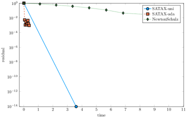
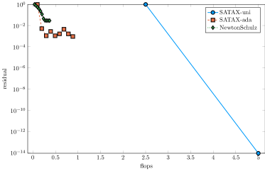
Figure 1: LPnetlib/lp_fit2d $(m;n)=(10,524;25)$.

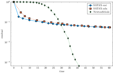
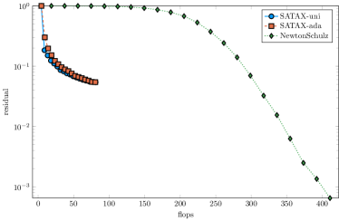
Figure 2: LPnetlib/lp_ken_07 $(m;n)=(2,426;3,602)$.

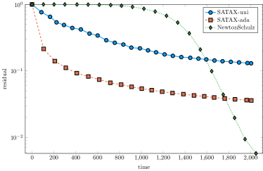
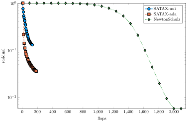
Figure 3: NYPA/Maragal_6 $(m;n)=(21,255;10,152)$.

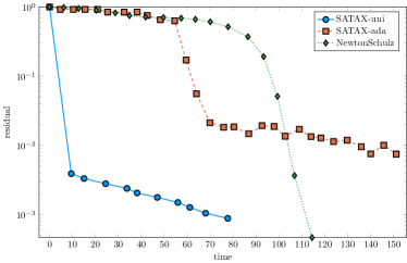
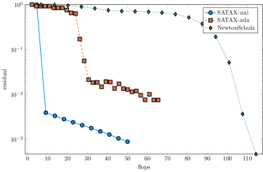
Figure 4: Meszaros/primagaz $(m;n)=(1,554;10,836)$

From Figure 1 we see that the SATAX methods are considerably faster at calculating the pseudoinverse on highly rectangular matrices ($n\ll m$ or $n\gg m$) as compared to the Newton-Schultz method. Indeed, by the time the Newton-Schultz method completes three iterations, the stochastic methods have already encountered a pseudoinverse within the desired accuracy. On the remaining problems in Figures 2, 3 and 4 the results are mixed, in that, the SATAX methods are very fast at encountering a rough approximation of the pseudoinverse with a residual between $10^{-1}$ and $10^{-3}$, but for reaching a lower residual the Newton-Schultz method proved to be the most efficient.

In calculating the approximate pseudoinverse of the the best rank $r=1000$ approximation to a random $5000\times 2500$ Gaussian matrix the Newton-Schultz method outperforms the randomized methods in terms of time taken but is less efficient is terms of flops, see in Figure 5. We observed this same result holds for Gaussian matrices with a range of different dimensions and different ranks.

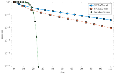
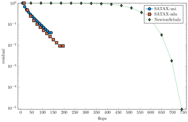
Figure 5: The matrix $A$ is the best rank $1000$ approximation to a randomly generated $5000\times 2500$ normal Gaussian matrix.

The faster initial convergence of SATAX methods and the local quadratic convergence of the Newton-Schulz method can be combined to create an efficient method. To illustrate, we create a combined method named NS-SATAX where we use the SATAX method for the first few iterations before switching to the Newton-Schulz method, see Figure 6. Through experiments we have identified that we should switch to the Newton-Schulz method after the SATAX method has performed one effective pass over the data. In other words, we should switch methods after $t$ iterations such that $t$ times the cost of computing the sketched matrix $AS$ is equal to the cost of performing one full matrix-matrix product $AX$ where $X\in\mathbb{R}^{n\times m}$. Though this requires care, in particular, if $X_{t}$ is the last iteration of the SATAX method, then we need to ensure that $X_{t}$ satisfies the starting condition $\lVert I-X_{t}A\rVert_{2}<1$ of the Newton-Schulz method. For this we normalize the iterate $X_{t}$ according to $X_{t}\leftarrow\left.X_{t}\right/\lVert X_{t}A\rVert_{F}.$ This normalization is a heuristic and is not guaranteed to satisfy the Newton-Schulz starting condition. Despite this, it does work in practice as we can see in Figure 6 where the combined method NS-SATAX outperforms the Newton-Schulz method during the entire execution.

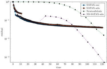
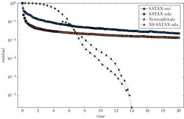
Figure 6: Comparing the new combined method NS-SATAX to the SATAX_uni, SATAX_ada and the Newton-Schulz method on the LPnetlib/lp_ken_07 matrix (LEFT figure) and the NYPA/Maragal_3 ( RIGHT figure).

5.2 Symmetric matrices

In this section we compare the SAXAS_uni, SAXAS_ada and Newton-Schulz methods. In setting the initial iterate $X_{0}$ for the SAXAS methods, we know from Lemma 7 and Theorem 6 that we need $X_{0}=\alpha A^{2}$ for some $\alpha\in\mathbb{R}$ to guarantee that the method converges. We choose $\alpha$ so that $\lVert X_{0}\rVert_{F}^{2}=1,$ that is $\alpha=\left.1\right/\lVert A\rVert_{F}^{2}.$

To test the symmetric methods we used the Hessian matrix $A^{\top}A$ of the linear regression problem

$$\min_{x\in\mathbb{R}^{n}}\frac{1}{2}\lVert Ax-b\rVert_{2}^{2}$$ (78)

using data from LIBSVM [7], see Figure 7, 8, 9 and 10. These experiments show that the two variants of the SAXAS method are much more efficient at calculating an approximate pseudoinverse as compared to the Newton-Schulz method, even for reaching a relative residual with a high precision of around $10^{-6}$. The only exception being the rcv1_train.binary problem in Figure 10, where the SAXAS_uni and SAXAS_ada methods make very good progress in the first few iterations, but then struggle to bring the residual much below $10^{-2}.$ Again looking at Figure 10, the trend appears that the Newton-Schulz method will reach a lower precision than the the SAXAS_uni and SAXAS_ada after approximately $4000$ seconds, though we were not prepared to wait so long. We leave it as an observation that we could again get the best of both worlds by combining an initial execution of the SAXAS methods and later switching to the Newton-Schulz method as was done with the SATAX and Newton-Schulz method in the previous section.

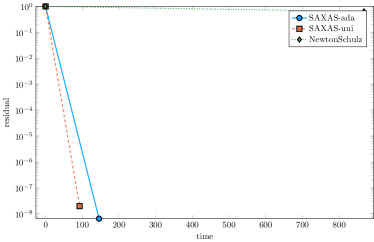
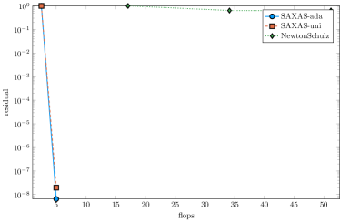
Figure 7: a9a: $(m;n)=(123;32,561)$.

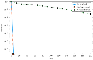
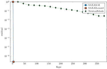
Figure 8: mushrooms: $(m;n)=(8,124;112)$

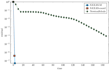
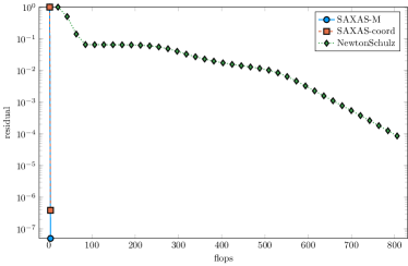
Figure 9: gisette_scale: $(m;n)=(6000;5000)$

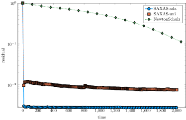
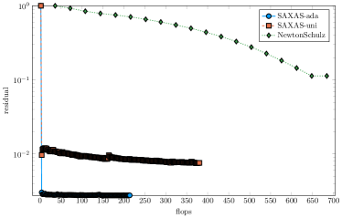
Figure 10: rcv1_train.binary: $(m;n)=(20,242;47,236)$

Again we found that the Newton-Schultz method was more efficient in calculating pseudoinverse of randomly generated Gaussian matrices $A$, where $A$ is the best rank $1000$ approximation to a matrix $G+G^{\top}$, where $G$ is a $5000\times 5000$ random Gaussian matrix; see Figure 11.

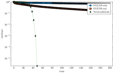
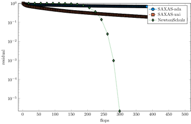
Figure 11: The matrix $A$ is the best rank $10^{3}$ approximation to the matrix $G+G^{\top}$ where $G$ is a $5000\times 5000$ random Gaussian matrix.

6 Conclusions and Future Work

We presented a new family of randomized methods for iteratively computing the pseudoinverse which are proven to converge linearly to the pseudoinverse matrix and, moreover, numeric experiments show that the new randomized methods are vastly superior at quickly obtaining an approximate pseudoinverse matrix. In such cases where an approximation of the pseudoinverse of a nonsymmetric matrix with a relative residual below $10^{-3}$ is required then our experiments show that the Newton Schultz method is more effective as compared to our randomized methods. These observations inspired a combined method which we illustrated in Figure 6 which has better overall performance than the Newton-Schulz method. Furthermore, we present new symmetric sketches used to design the SAXAS method. For future work, we have indicated how to design randomized methods for calculating approximate range space projections and pseudoinverse of full rank matrices.

7 Appendix

Here we present and prove several fundamental linear algebra lemmas that are required to develop the main theorems in the paper.

7.1 Key linear algebra lemmas

Lemma 13

For any matrix $W$ and symmetric positive semidefinite matrix $G$ such that

$$\mathbf{Null}\left(G\right)\subset\mathbf{Null}\left(W^{\top}\right),$$ (79)

we have that

$$\mathbf{Null}\left(W\right)=\mathbf{Null}\left(W^{\top}GW\right)$$ (80)

and

$$\mathbf{Range}\left(W^{\top}\right)=\mathbf{Range}\left(W^{\top}GW\right).$$ (81)

Proof: In order to establish (80), it suffices to show the inclusion $\mathbf{Null}\left(W\right)\supseteq\mathbf{Null}\left(W^{\top}GW\right)$ since the reverse inclusion trivially holds. Letting $s\in\mathbf{Null}\left(W^{\top}GW\right)$, we see that $\|G^{1/2}Ws\|^{2}=0$, which implies $G^{1/2}Ws=0$. Consequently

$$Ws\in\mathbf{Null}\left(G^{1/2}\right)=\mathbf{Null}\left(G\right)\overset{\eqref{eq:Gnullassm}}{\subset}\mathbf{Null}\left(W^{\top}\right).$$

Thus $Ws\in\mathbf{Null}\left(W^{\top}\right)\cap\mathbf{Range}\left(W\right)$ which are orthogonal complements which shows that $Ws=0.$

Finally, (81) follows from (80) by taking orthogonal complements. Indeed, $\mathbf{Range}\left(W^{\top}\right)$ is the orthogonal complement of $\mathbf{Null}\left(W\right)$ and $\mathbf{Range}\left(W^{\top}GW\right)$ is the orthogonal complement of $\mathbf{Null}\left(W^{\top}GW\right)$.       

The following two lemmas are of key importance throughout the paper.

Lemma 14

For any matrix $M\in\mathbb{R}^{m\times n}$ and any matrix $R\in\mathbb{R}^{n\times d}$ such that $\mathbf{Range}\left(R\right)\subset\mathbf{Range}\left(M^{\top}\right)$ we have that

$$\left<M^{\top}MR,R\right>\geq\lambda_{\min}^{+}(M^{\top}M)\left<R,R\right>,$$ (82)

Proof: Since

$$\left<M^{\top}MR,R\right>=\mathbf{Tr}\left(R^{\top}M^{\top}MR\right)=\sum_{i=1}^{d}\left<M^{\top}MR_{:i},R_{:i}\right>,$$

the inequality (82) follows from the known inequality

$$\left<M^{\top}Mv,v\right>\geq\lambda_{\min}^{+}(M^{\top}M)\left<v,v\right>,$$

where $v\in\mathbf{Range}\left(M^{\top}\right),$ which can be proved be diagonalizing $M^{\top}M.$

Lemma 15

Let $0\neq W\in\mathbb{R}^{m\times n}$ and $G\in\mathbb{R}^{m\times m}$ be symmetric positive semi-definite with $\mathbf{Null}\left(G\right)\subset\mathbf{Null}\left(W^{\top}\right)$. Then the matrix $W^{\top}GW$ has a positive eigenvalue, and the following inequality holds:

$$\left<W^{\top}GWR,R\right>\geq\lambda_{\min}^{+}(W^{\top}GW)\left<R,R\right>,$$ (83)

where $R$ is a matrix with $n$ rows and $\mathbf{Range}\left(R\right)\subset\mathbf{Range}\left(W^{\top}\right).$

Proof: By Lemma 14 with $M=G^{1/2}W$ we have that (83) holds for $\mathbf{Range}\left(R\right)\subset\mathbf{Range}\left(W^{\top}G^{1/2}\right).$ The proof now follows by observing

$$\mathbf{Range}\left(W^{\top}G^{1/2}\right)\overset{\text{Lemma}~{}\ref{lem:09709s}}{=}\mathbf{Range}\left(W^{\top}GW\right)\overset{\text{Lemma}~{}\ref{lem:09709s}}{=}\mathbf{Range}\left(W^{\top}\right).\hfill\nobreak\hskip 0.0pt\hskip 15.00002pt minus 5.0pt\nobreak\vrule height=7.5pt,width=5.0pt,depth=2.5pt$$

7.2 Smallest nonzero eigenvalue of the product of two matrices

Lemma 16

Let $A,B\in\mathbb{R}^{n\times n}$ be symmetric positive semidefinite matrices. If

$$\mathbf{Null}\left(A\right)\subset\mathbf{Null}\left(B\right)$$ (84)

then

$$\lambda_{\min}^{+}(AB)\geq\lambda_{\min}^{+}(A)\lambda_{\min}^{+}(B).$$ (85)

Proof: Using the variational formulation we have that

$$\lambda_{\min}^{+}(AB) = \min_{v\in\mathbf{Null}\left(AB\right)^{\perp}}\frac{\lVert ABv\rVert}{\lVert v\rVert}$$ (86)

$$= \min_{v\in\mathbf{Null}\left(AB\right)^{\perp}}\frac{\lVert ABv\rVert}{\lVert Bv\rVert}\frac{\lVert Bv\rVert}{\lVert v\rVert}$$

$$\leq \min_{v\in\mathbf{Null}\left(AB\right)^{\perp}}\frac{\lVert ABv\rVert}{\lVert Bv\rVert}\min_{v\in\mathbf{Null}\left(AB\right)^{\perp}}\frac{\lVert Bv\rVert}{\lVert v\rVert}.$$

Given that

$$\mathbf{Null}\left(B\right)\subset\mathbf{Null}\left(AB\right)$$

ergo

$$\mathbf{Null}\left(AB\right)^{\perp}\subset\mathbf{Null}\left(B\right)^{\perp}\overset{\eqref{eq:NullANullB}}{\subset}\mathbf{Null}\left(A\right)^{\perp}.$$

The above shows that

$$\min_{v\in\mathbf{Null}\left(AB\right)^{\perp}}\frac{\lVert Bv\rVert}{\lVert v\rVert}\geq\min_{v\in\mathbf{Null}\left(B\right)^{\perp}}\frac{\lVert Bv\rVert}{\lVert v\rVert}=\lambda_{\min}^{+}(B).$$ (87)

But also, since $\mathbf{Null}\left(B\right)^{\perp}=\mathbf{Range}\left(B\right)=\mathbf{Range}\left(BB\right)$ which follows from $B$ being symmetric and Lemma 13, we have that

$$\min_{v\in\mathbf{Null}\left(AB\right)^{\perp}}\frac{\lVert ABv\rVert}{\lVert Bv\rVert} \geq \min_{v\in\mathbf{Range}\left(B\right)}\frac{\lVert ABv\rVert}{\lVert Bv\rVert}$$ (88)

$$= \min_{w\in\mathbf{Range}\left(BB\right)}\frac{\lVert Aw\rVert}{\lVert w\rVert}$$

$$= \min_{w\in\mathbf{Range}\left(B\right)}\frac{\lVert Aw\rVert}{\lVert w\rVert}=\lambda_{\min}^{+}(A).$$

Inserting (87) and (88) in (86) gives the desired result.

7.3 Convenient probability lemma

Theorem 17

Let $G$ be a positive symmetric semidefinite matrix. Let $S$ be a random matrix with a finite discrete distribution with $r$ $S=S_{i}\in\mathbb{R}^{n\times q_{i}}$ with probability $p_{i}>0$ for $i=1,\ldots,r$. Let $\mathbb{S}\overset{\text{def}}{=}[S_{1},\ldots,S_{r}]\in\mathbb{R}^{n\times n}$. If

$$p_{i}~{}=~{}\dfrac{\mathbf{Tr}\left(S_{i}^{\top}G^{2}S_{i}\right)}{\mathbf{Tr}\left(\mathbb{S}^{\top}G^{2}\mathbb{S}\right)},\quad\mbox{for }\quad i=1,\ldots,{r}.$$ (89)

then

$$\lambda_{\min}^{+}\left(G\mathbf{E}\left[S(S^{\top}G^{2}S)^{\dagger}S^{\top}\right]G\right)\quad\geq\quad\frac{\lambda_{\min}^{+}\left(\mathbb{S}^{\top}G^{2}\mathbb{S}\right)}{\mathbf{Tr}\left(\mathbb{S}^{\top}G^{2}\mathbb{S}\right)}.$$ (90)

Proof: Let $Z=GS(S^{\top}G^{2}S)^{\dagger}S^{\top}G.$ Note that

$$\mathbf{E}\left[Z\right]=G\mathbb{S}D\mathbb{S}^{\top}G,$$ (91)

with

$$D\quad\overset{\text{def}}{=}\quad\mbox{diag}(p_{i}(S^{\top}G^{2}S)^{\dagger}).$$ (92)

Let $t_{i}=\mathbf{Tr}\left(S_{i}^{\top}G^{2}S_{i}\right)$, and with (89) in (92) we have

$$D=\frac{1}{\mathbf{Tr}\left(\mathbb{S}^{\top}G^{2}\mathbb{S}\right)}\mbox{diag}\left(t_{1}(S_{1}^{\top}G^{2}S_{1})^{\dagger},\ldots,t_{r}(S_{r}^{\top}G^{2}S_{r})^{\dagger}\right),$$

thus

$$\lambda_{\min}^{+}(D)=\frac{1}{\mathbf{Tr}\left(\mathbb{S}^{\top}G^{2}\mathbb{S}\right)}\min_{i\,:\,t_{i}\neq 0}\left\{\frac{t_{i}}{\lambda_{\max}(S_{i}^{\top}G^{2}S_{i})}\right\}\geq\frac{1}{\mathbf{Tr}\left(\mathbb{S}^{\top}G^{2}\mathbb{S}\right)}.$$ (93)

Thus

$$\lambda_{\min}^{+}\left(\mathbf{E}\left[Z\right]\right) \overset{\eqref{eq:EZlemappend}}{=} \lambda_{\min}^{+}\left(G\mathbb{S}D\mathbb{S}^{\top}G\right)$$ (94)

$$= \lambda_{\min}^{+}\left(D\mathbb{S}^{\top}GG\mathbb{S}\right)$$

$$\overset{\text{Lemma}~{}\ref{lem:prodsmallest}}{\geq} \frac{\lambda_{\min}^{+}\left(\mathbb{S}^{\top}GG\mathbb{S}\right)}{\mathbf{Tr}\left(\mathbb{S}^{\top}G^{2}\mathbb{S}\right)},$$

where in the second line we used that, for any matrices $A,B$, the matrices $AB$ and $BA$ share the same nonzero eigenvalues.

References

- [1] Y. Hel-Or A. Adler and M. Elad. A weighted discriminative approach for image denoising with overcomplete representations. IEEE International Conference on Acoustics, Speech, and Signal Processing (ICASSP), Dallas, TX, 14-19 March, March 2010.
- [2] Adi Ben-Israel. An iterative method for computing the generalized inverse of a matrix. Mathematics of Computation, 19(91):452–455, 1965.
- [3] Adi Ben-Israel and Dan Cohen. On iterative computation of generalized inverses and associated projections. SIAM Journal on Numerical Analysis, 3(3):410–419, 1966.
- [4] Michele Benzi and Miroslav Tůma. Comparative study of sparse approximate inverse preconditioners. Applied Numerical Mathematics, 30(2–3):305–340, 1999.
- [5] C. G. Broyden. Quasi-Newton methods and their application to function minimisation. Mathematics of Computation, 21(99):368–381, 1967.
- [6] Paul H. Calamai and Jorge J. Moré. Projected gradient methods for linearly constrained problems. Mathematical Programming, 39(1):93–116, 1987.
- [7] Chih Chung Chang and Chih Jen Lin. LIBSVM : A library for support vector machines. ACM Transactions on Intelligent Systems and Technology, 2(3):1–27, April 2011.
- [8] Edmond Chow and Yousef Saad. Approximate inverse preconditioners via sparse-sparse iterations. SIAM Journal of Scientific Computing, 19(3):995–1023, 1998.
- [9] Timothy A. Davis and Yifan Hu. The University of Florida sparse matrix collection. ACM Transactions on Mathematical Software, 38(1):1:1–1:25, 2011.
- [10] Ron S. Dembo, Stanley C. Eisenstat, and Trond Steihaug. Inexact Newton methods. SIAM Journal on Numerical Analysis, 19(2):400–408, 1982.
- [11] C. A. Desoer and B. H. Whalen. A note on pseudoinverses. Journal of the Society of Industrial and Applied Mathematics, 11(2):442–447, 1963.
- [12] Hans G. Feichtinger. Pseudoinverse matrix methods for signal reconstruction from partial data. Proc. SPIE, Visual Communications and Image Processing ’91, 1606:766–772, 1991.
- [13] Jacek Gondzio. Convergence analysis of an inexact feasible interior point method for convex quadratic programming. SIAM Journal on Optimization, 23(3):1510–1527, 2013.
- [14] N. I. M. Gould, M. E. Hribar, and J. Nocedal. On the solution of equality constrained quadratic problems arising in optimization. SIAM Journal on Scientific Computing, 23(4):1375–1394, 2001.
- [15] Nicholas I. M. Gould and Jennifer A. Scott. Sparse approximate-inverse preconditioners using norm-minimization techniques. SIAM Journal on Scientific Computing, 19(2):605–625, 1998.
- [16] Robert M. Gower. Sketch and Project: Randomized Iterative Methods for Linear Systems and Inverting Matrices. PhD thesis, University of Edinburgh, 2016.
- [17] Robert M. Gower, Donald Goldfarb, and Peter Richtárik. Stochastic block BFGS: Squeezing more curvature out of data. Proceedings of the 33rd International Conference on Machine Learning, 2016.
- [18] Robert M. Gower and Peter Richtárik. Stochastic dual ascent for solving linear systems. arXiv:1512.06890, 2015.
- [19] Robert Mansel Gower and Peter Richtárik. Randomized iterative methods for linear systems. SIAM Journal on Matrix Analysis and Applications, 36(4):1660–1690, 2015.
- [20] Robert Mansel Gower and Peter Richtárik. Randomized quasi-Newton updates are linearly convergent matrix inversion algorithms. arXiv:1602.01768, 2016.
- [21] Marcus J. Grote and Thomas Huckle. Parallel preconditioning with sparse approximate inverses. SIAM J. Sci. Comput, 18:838–853, 1996.
- [22] Nicolas Loizou and Peter Richtárik. A new perspective on randomized gossip algorithms. In 4th IEEE Global Conference on Signal and Information Processing (GlobalSIP), 2016.
- [23] E. H. Moore. Abstract for “On the reciprocal of the general algebraic matrix”. Bulletin of the American Mathematical Society, 26:394–395, 1920.
- [24] Victor Pan and Robert Schreiber. An improved newton iteration for the generalized inverse of a matrix, with applications. SIAM J. Scientific Computing, 12(5):1109–1130, 1991.
- [25] R. Penrose. A generalized inverse for matrices. Mathematical Proceedings of the Cambridge Philosophical Society, 51(3):406–413, 1955.
- [26] Gregory Robertson, R. Lynn Kirlin, and W. S. Lu. A pseudoinverse update algorithm for rank-reduced covariance matrices from 2-d data. IEEE Signal Processing Letters, 3, 1997.
- [27] Thomas Strohmer and Roman Vershynin. A randomized Kaczmarz algorithm with exponential convergence. Journal of Fourier Analysis and Applications, 15(2):262–278, 2009.
- [28] J. Tapson and A. Van Schaik. Learning the pseudoinverse solution to network weights. Neural Networks, 45:94–100, September 2013.