An eccentric companion at the edge of the brown dwarf desert orbiting the 2.4 M_⊙ giant star HIP 67537.

We report the discovery of a substellar companion around the giant star HIP 67537. Based on precision radial velocity measurements from CHIRON and FEROS high-resolution spectroscopic data, we derived the following orbital elements for HIP 67537 $b$: m_b sin$i$= 11.1${}^{+0.4}_{-1.1}$ M_jup , $a$ = 4.9${}^{+0.14}_{-0.13}$ AU and $e$ = 0.59${}^{+0.05}_{-0.02}$. Considering random inclination angles, this object has $\gtrsim$ 65% probability to be above the theoretical deuterium-burning limit, thus it is one of the few known objects in the planet to brown-dwarf transition region. In addition, we analyzed the Hipparcos astrometric data of this star, from which we derived a minimum inclination angle for the companion of $\sim$ 2 deg. This value corresponds to an upper mass limit of $\sim$ 0.3 M_⊙ , therefore the probability that HIP 67537 $b$ is stellar in nature is $\lesssim$ 7%. The large mass of the host star and the high orbital eccentricity makes HIP 67537 $b$ a very interesting and rare substellar object. This is the second candidate companion in the brown dwarf desert detected in the sample of intermediate-mass stars targeted by the EXPRESS radial velocity program, which corresponds to a detection fraction of $f$ = 1.6${}^{+2.0}_{-0.5}$ %. This value is larger than the fraction observed in solar-type stars, providing new observational evidence of an enhanced formation efficiency of massive substellar companions in massive disks. Finally, we speculate about different formation channels for this object.

1 Introduction

So far, more than 2000 exoplanets have been detected and confirmed, most of these via radial velocity (RV) time-series and transit observations, and thousands of new candidates from the space mission Kepler that still await confirmation. Soon after the discovery of the first extra-solar planets, several interesting observational results emerged, some of which were unexpected, showing us that planetary systems are quite common and are found to have a large diversity of orbital configurations. In particular, the early discovery of a large population of Hot-Jupiters (including the 51 Peg system; Mayor & Queloz MAY95 (1995)), the planet-metallicity correlation (Gonzalez GON97 (1997)), and the observed high eccentricity systems, among others, gave us important clues about the formation mechanisms and evolution of planetary systems. In addition, RV surveys have also revealed the intriguing paucity of brown dwarf (BD) companions to solar-type stars with orbital separation $\lesssim$ 3 - 5 AU (Marcy & Butler MAR00 (2000); Marcy et al. MAR05 (2005); Grether & Lineweaver GRE06 (2006); Sahlmann et al. SAH11 (2011)), dubbed the brown dwarf desert.
According to the IAU definition (Boss et al. BOS03 (2003)), a BD corresponds to a substellar object that is massive enough to burn deuterium, but it is not able to sustain Hydrogen fusion in its core. In terms of mass, these limits correspond to $\sim$ 13 - 80  M_jup , for a solar composition (Chabrier & Baraffe CHA97 (1997); Burrows et al. BUR01 (2001)). Although the upper mass limit is well justified, there is no physical reason to adopt the deuterium-burning limit as a discriminant between planets and brown dwarfs. Moreover, it has been argued that these types of substellar objects should be distinguished by their formation mechanism, which seems to have separate channels (Chabrier et al. CHA14 (2014); Ma & Ge MA14 (2014)). For instance, the fraction of giant planets (M_p $\gtrsim$ 0.5 M_jup ) with $a\lesssim$ 5 AU increases from $f$ = 2.5 $\pm\,$0.9 % around M dwarfs (Johnson et al. JOHN10 (2010)) to $f$ = 6.6 $\pm$ 0.7 % for solar-type stars (Marcy et al. MAR05 (2005); Johnson et al. JOHN10 (2010)). This fraction reaches a maximum value of 13.0${}^{+10.1}_{-4.1}$ %, at $\sim$ 2 M_⊙ (Jones et al. JON16 (2016)). Similarly, Reffert et al. (REF15 (2015)) found a peak in the detection fraction at M_⋆= 1.9${}^{+0.1}_{-0.5}$ M_⊙ . In addition, it is now well established that the fraction of giant planets around solar-type stars increases with the stellar metallicity (Santos et al. SAN01 (2001); Fischer & Valenti FIS05 (2005); Jenkins et al. JEN17 (2017)), which has been shown to be also valid for giant (intermediate-mass) stars (Reffert et al. REF15 (2015); Jones et al. JON16 (2016); Wittenmyer et al. WIT17 (2017)). These trends are in accordance with the core-accretion formation model of giant planets (Pollack et al. POL96 (1996); Alibert et al. ALI04 (2004); Kennedy & Kenyon KEN08 (2008)). In contrast, BD companions are rarely found around solar-type stars interior to $\sim$ 5 AU ($f$ $\lesssim$ 0.6 %; Marcy & Butler MAR00 (2000); Sahlmann et al. SAH11 (2011)) and also there is no clear dependence between the host star metallicity and the detection rate of such objects (although searching for such a correlation in the BD host stars is hampered by the very low detection rate of such objects). In this context, it seems reasonable to believe that giant planets are efficiently formed via core-accretion in the protoplanetary disk, while BDs are born akin to low-mass stars, by molecular cloud fragmentation (Luhman et al. LUH07 (2007); Joergens JOE08 (2008)), and thus we might expect an overlapping mass (transition) region, in which both of these formation channels take place. Therefore, the detection and characterization of planet to BD transition objects is of key importance to better understand the thin transition regime between the high-mass planetary tail and the low-mass brown dwarf regime. In particular, the mass and metallicity of the parent star certainly gives us important clues regarding the formation mechanism of such objects.
In this paper we present precision RVs of the intermediate-mass evolved star HIP 67537, revealing the presence of a substellar object in the transition limit between giant planets and BDs. The host star is one of the targets of the EXoPlanets aRound Evolved StarS (EXPRESS) radial velocity program (Jones et al. JON11 (2011)). Also, we analyzed the Hipparcos astrometric data of HIP 67537 from which we derived an upper mass limit for its companion. Finally, we discuss about the fraction of companions in the brown dwarf desert around intermediate-mass stars and we speculate on the different scenarios that might explain the formation and orbital evolution of this system. The paper is organized as follows: In section 2 the observations, data reduction and orbital solution are presented. In section 3 we present in detail our new codes that we use to compute the radial velocities, for both the simultaneous calibration method and the I₂ cell technique. In section 4 we present the physical properties of HIP 67537, while its companion orbital elements are presented in section 5. In section 6, we present a detailed study of the photometric variability, bisector analysis and chromospheric stellar activity of the host stars. In section 7 we analyze the Hipparcos astrometric data of HIP 67537 and its companion upper mass limit. Finally, the summary and discussion is presented in section 8.

2 Observations and data reduction

The observations were performed with the FEROS (Kaufer et al. KAU99 (1999)) and CHIRON (Tokovinin et al. TOK13 (2013)) high-resolution optical spectrographs. FEROS is equipped with two fibres, one for the science object and the second one for simultaneous calibration, which is used to track and correct the spectral drift during the observations (see Baranne et al. BAR96 (1996)). The reduction of the FEROS data was done in the standard fashion (i.e, bias subtraction, flat-field correction, order-by-order extraction and wavelength calibration) using the CERES reduction code (Jordán et al. JOR14 (2014); Brahm et al. BRA16 (2016)). On the other hand, CHIRON is equipped with an iodine cell, which is located in the light path, in front of the fibre entrance in the spectrograph. The I₂ vapor inside the cell absorbs part of the incoming light, producing a rich narrow absorption spectrum that is superimposed onto the stellar spectrum, in the range between $\sim$ 5000-6200 Å. We use the CHIRON pipeline to obtain order-by-order wavelength calibrated spectra. We typically use the fiber slicer, which delivers a spectral resolution of $\sim$ 80,000, and much higher efficiency compared to the slit (R$\sim$ 90,000) and narrow slit mode (R$\sim$ 130,000).

3 Radial velocities

We have recently developed new radial velocity analysis codes for both FEROS and CHIRON data. In the two cases, we have reduced our internal RV uncertainties by up to a factor two. Additionally, we have developed automatic stellar activity diagnoses that are included in these new pipelines. The new main features and differences with the old codes (e.g. Jones et al. JON13 (2013); Jones & Jenkins JON14 (2014)) are discussed in the following sections.

3.1 FEROS data

The FEROS radial velocity variations were computed using the cross-correlation technique (Tonry & Davis TON79 (1979)), with a new dedicated IDL-based pipeline, which is more flexible and user-friendly that our old IRAF and Fortran based codes used for this purpose (Jones et al. JON13 (2013)). We compute the cross-correlation function (CCF) between a high S/N template, which is created by stacking all of the FEROS spectra of each star, after correcting by their relative velocity offset, and each observed spectrum. We then fit the CCF by a Gaussian plus a linear function. We note that the addition of the linear term improves our results when compared to the single Gaussian CCF model. The maximum of the fit corresponds to the wavelength (velocity) shift. This method is applied to a total of 100 chunks per spectrum, each of $\sim$ 50 Å  in length, across 25 different orders, covering the wavelength range of $\sim$ 3900 - 6700 Å. Then, deviant chunk velocities are filtered-out using a 3-$\sigma$ iterative rejection method. The velocity shift per epoch is computed from the median of the non-rejected chunk velocities and its uncertainty corresponds to the formal error in the mean. We note that we use the median instead of the mean because it leads to slightly better results in terms of long-term stability observed in the RV standard star $\tau$ Ceti. A similar procedure is computed for the simultaneous calibration lamp. However, in this case the template corresponds to the lamp observation that is used to compute the wavelength solution. The final velocities are obtained after correcting the night drift recorded by the simultaneous lamp and the barycentric correction, which is computed at the mid-time of the observation (FEROS is not equipped with an exposure meter). We note that we assign a constant weight to all of the non-rejected chunks. We tried different weighting scenarios based on different combinations of the CCF parameters (height and width), but no improvement in the final velocities was observed. Figure 1 shows 57 FEROS RV epochs spanning a total of 5.5 years of the standard RV star $\tau$ Ceti. The mean internal uncertainty is 3.8 m s^-1 . The long-term stability is 5.3 m s^-1 , which is superior to the value of $\sim$ 10 m s^-1 (restricting to the observations taken after 2010) obtained with the ESO data reduction system for FEROS (Soto et al. SOT15 (2015)).

3.2 CHIRON data

The CHIRON velocity variations were computed using a similar method as presented in Butler et al. (BUT96 (1996)), however we use a simpler PSF model, including only one Gaussian (being the width of the Gaussian a free parameter), which yields nearly identical results to the multi-Gaussian models. Also, we compute the radial velocities for a total of 352 chunks, each of 180 pixels, spread over 22 different orders. The resulting velocity at each epoch is obtained from the median in the individual chunks velocities, after passing an iterative rejection procedure, in a similar fashion as done for the FEROS data. The typical RV precision that we achieve is $\sim$ 3 m s^-1 for slit observations (R $\sim$ 90,000) and $\sim$ 4 m s^-1 using the image slicer ( R $\sim$ 80,000). We note that it is possible to achieve a precision $\sim$ 2 m s^-1 applying the single-Gaussian model to high signal-to-noise (S/N) ratio observations using the narrow-slit mode (R$\sim$ 130,000), but at a cost of much higher exposure times due to the reduced efficiency. In particular, the RV precision is highly dependent on the quality of the stellar template, which is constructed via PSF deconvolution of a I₂-free observation of the star. However, due to the intrinsic p-modes induced RV variability of all of our targets (typically at the $\sim$ 5-10 m s^-1 level; see Kjeldsen & Bedding KJE95 (1995)), we have adopted the image slicer mode, which provides higher throughput compared to the slit modes and allow us to achieve instrumental uncertainties below the stellar noise level.

Figure 1: 5.5 years of FEROS observations of the RV standard star $\tau$ Ceti. The mean internal error is 3.8 m s^-1 , while the long-term RMS around the mean is 5.3 m s^-1 .

4 HIP 67537 properties

The fundamental parameters of HIP 67537 are listed in Table 1. The visual magnitude, B-V color, and the corresponding errors were computed from the linear transformations between the Tycho and Johnson photometric systems, as given in section 1.3 of the Hipparcos and Tycho Catalogs (ESA, ESA97 (1997)). The distance to the star was computed using the parallax listed in the new data reduction of the Hipparcos data (Van Leeuwen, VAN07 (2007)). We note that no parallax for HIP 67537 is available from the GAIA DR1. We corrected the visual magnitude using the Arenou et al. (ARE92 (1992)) extinction maps and applied the Alonso et al. (ALO99 (1999)) bolometric correction to obtain the stellar luminosity. The atmospheric parameters, namely T_eff, logg and [Fe/H], were derived using the equivalent width ($W$) of a carefully selected list of $\sim$ 150 Fe i and $\sim$ 20 Fe ii relatively weak lines ($W\,\lesssim$ 150 Å ), which were measured using the ARES code (Sousa et al. SOU07 (2007)). For this purpose, we used MOOG (Sneden SNE73 (1973)), which solves the radiative transfer equation, imposing local excitation and ionization equilibrium. Briefly, for a given set of atmospheric parameters, MOOG computes the iron abundance corresponding to each measured equivalent width, by matching the curve of growth in the weak line regime, and including the effect of the micro-turbulence. The final atmospheric parameters are thus obtained in an iterative process, by removing any dependence between the abundance with the excitation potential and reduced equivalent widths ($W/\lambda$), and also by forcing the iron abundance to be the same from both species (Fe i and Fe ii). For a detailed description of this method see (Gray GRAY05 (2005)). The resulting atmospheric parameters of HIP 67537 are listed in Table 1. For comparison, Alves et al. (ALV15 (2015)), based o a similar approach, obtained the following parameters: T_eff = 5017 $\pm$ 042 K, log$g$ = 3.08 $\pm$ 0.08 cm s^-2 and [Fe/H] = 0.17 $\pm$ 0.03 dex. These results are in good agreement with those presented here. Finally, the stellar position in the H-R diagram and the derived metallicity were compared with Salasnich et al. (SAL00 (2000)) evolutionary tracks, to obtain the stellar mass and radius. This procedure was repeated 100 times, from random generated datasets, assuming Gaussian distributed errors in the luminosity, effective temperature and stellar metallicity. The adopted values for M_⋆  and R_⋆, and their corresponding uncertainties, were obtained from the mean and standard deviation in the resulting distribution from the 100 random samples. For further details see Jones et al. (JON11 (2011); 2015b )

5 Orbital elements of HIP 67537 $b$

We obtained a total of 19 FEROS spectra and 18 CHIRON observations of HIP 67537, covering a total baseline of more than 6 years. In addition, we retrieved a FEROS observation from the ESO archive, which was taken in 2004, but without simultaneous calibration. However, since FEROS is relatively stable the spectral drift was computed from three RV stable stars that were observed before and after HIP 67537. The night drift was then interpolated to the time of the observation of HIP 67537. We note that we have applied this method to FEROS data of HIP 67851 (which were taken immediately after HIP 67537) to constrain the orbital period of HIP 67851 $c$ (Jones et al. 2015b ). New RV measurements of HIP 67851 (which already cover one orbital period of HIP 67851 $c$) confirm the validity of this method. The resulting radial velocities are listed in Table 1 and are shown in Figure 2. As can be seen, the peak-to-peak variation exceeds 200 m s^-1 , which is indicative of the presence of a massive substellar object. The orbital elements of the companion were obtained with the Systemic Console (Meschiari et al. MES09 (2009)), after adding 7 m s^-1 RV noise in quadrature to the radial velocities, which is the typical level of RV scatter observed in our sample. The resulting values are listed in Table 1. The uncertainties were derived using the bootstrap tool included in version 2.17 of Systemic and correspond to the 1-$\sigma$ equal-tailed confidence interval. The best Keplerian fit is overplotted in Figure 2. The RMS about the best fit is 8.0 m s^-1 . We note that no significant improvement in the Keplerian fit is obtained by including a linear trend in the solution and no significant periodicity is present in the post-fit residuals (see Figure 3).

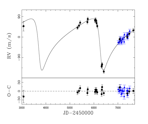
Figure 2: Radial velocity measurements of HIP 67537. The black circles and blue triangles represent the FEROS and CHIRON velocities, respectively. The best Keplerian solution is overplotted (black solid line). The post-fit residuals are shown in the lower panel.

Figure 3: Lomb-Scargle periodogram of the post-fit residuals of the HIP 67537 velocities.

Table 1: Stellar properties and orbital elements.

Stellar properties of HIP 67537
Spectral Type	K1III
$B-V$ (mag)	0.99 $\pm$ 0.006
$V$ (mag)	6.44 $\pm$ 0.005
Distance (pc)	112.6 $\pm$ 5.8
Teff (K)	4985 $\pm$ 100
Luminosity (L⊙)	41.37 $\pm$ 7.16
log $g$ (cm s-2)	2.85 $\pm$ 0.2
[Fe/H] (dex)	0.15 $\pm$ 0.08
$v$ sin$i$ (km s-1 )	2.3 $\pm$ 0.9
M⋆ (M⊙ )	2.41 $\pm$ 0.16
R⋆ (R⊙)	8.69 $\pm$ 0.88
Orbital parameters of HIP 67537 b
P (days)	2556.5${}^{+99.2}_{-94.9}$
K (m s-1 )	112.7${}^{+7.8}_{-3.0}$
$a$ (AU)	4.91${}^{+0.14}_{-0.13}$
$e$	0.59${}^{+0.05}_{-0.02}$
mb sin$i$  (Mjup )	11.1${}^{+0.4}_{-1.1}$
$\omega$ (deg)	119.6${}^{+4.6}_{-6.7}$
TP (JD-2450000)	6290.6${}^{+16.2}_{-51.6}$
$\gamma_{1}$ (m s-1 ) (FEROS)	11.0${}^{+3.8}_{-3.8}$
$\gamma_{2}$ (m s-1 ) (CHIRON)	-6.1${}^{+3.7}_{-3.7}$
RMS (m s-1 )	8.0
$\chi$${}^{2}_{\rm red}$	1.0

6 Planet validation

Stellar phenomena such as non-radial pulsations, spots and plages in rotating stars and other activity-related effects (like suppression of the convective blueshift in active regions), might produce apparent RV variations, mainly via CCF deformation, that can mimic the effect of a genuine doppler signal induced by an orbiting companion (e.g. Saar & Donahue SAR97 (1997); Huélamo et al. HUE08 (2008); Meunier et al. MEU10 (2010); Dumusque et al. DUM11 (2011)). In the following sections we analyze the available Hipparcos photometric data, we present a study of the CCF asymmetry variations and a chromospheric activity analysis, to understand whether the RV variations observed in HIP 67537 are explained by intrinsic stellar phenomena, like those discussed above.

6.1 Photometric analysis

We analyzed the Hipparcos photometry of HIP 67537, to investigate a possible correlation with the radial velocities. This dataset consists of a total of 94 good quality measurements (quality flag equal to 0 and 1), covering a time span of 1164 days, which is is significantly shorter than the orbital period, thus it is not possible to search for periodic photometric signals with similar periods than the orbital one. However, the data present a variability of only 0.006 mag (corresponding to $\sim$ 0.6% in flux), which is too small to explain the large velocity variations observed in slow rotating stars like HIP 67537 (Hatzes HAT02 (2002); Boisse et al. BOI12 (2012)). Moreover, in this scenario we would expect the radial velocity period to match the stellar rotational period, which is clearly not the case. Based on the measured $v$ sin $i$ and R_⋆ (see Table 1), we expect a maximum stellar rotational period of $\sim$ 191 days, which is $\sim$ 15 times shorter than the observed orbital period. Therefore, we discard rotational modulation as the cause of the observed RV variations.
Additionally, to test for possible light contribution from the unseen companions, we used Johnson, GENEVA and 2MASS photometric data from the literature. The fitting procedure used is the binary SED fit outlined in Vos et al. (VOS12 (2012, 2013)), in which the parameters of the giant component are kept fixed (to those listed in Table 1), while companion parameters are varied. Furthermore, the Hipparcos parallax is used as an extra constraint. For this procedure, five photometric points are enough for a reliable result (e.g. Bluhm et al. BLU16 (2016)). The observed photometry is fitted with a synthetic SED integrated from the Kurucz (KUR79 (1979)) atmosphere models ranging in effective temperature from 3000 to 7000 K, and in surface gravity from $\log{g}$=2.0 dex (cgs) to 5.0 dex (cgs). The radius of the companion is varied from 0.1 R_⊙ to 2.0 $R_{\odot}$. The SED fitting procedure uses the grid based approach described in Degroote et al. (DEG11 (2011)), where 10⁶ models are randomly picked in the available parameter space. The best fitting model is determined based on the $\chi^{2}$ value. As the parameters (effective temperature, surface gravity and radius) of the giant component are fixed at the values determined from the spectroscopy, and the distance to these systems is known accurately from the Hipparcos parallax, the total luminosity of the giant is fixed. This allows to accurately determine the amount of extra light from the companion, based on the SED fit. For this system, this is less than 1%, which is within the uncertainties of the SED fit. We can thus conclude that no significant light contribution from the companion is observed in this system. As an extra test, an unconstrained SED fit was performed, in which the atmospheric parameters of the giant were varied. This provides an independent set of atmospheric parameters. We find that in both cases the atmospheric parameters of the best fitting SED models correspond well with those derived from spectroscopy. We found no indication of contamination from an unseen companion.

6.2 Line asymmetry

We computed the bisector velocity span (BVS) of the CCF (Toner & Gray TON88 (1988)), as a stellar line asymmetry indicator, since spots in a rotating star and non-radial pulsations propagating in the stellar surface can produce significant distortions in the observed stellar spectral lines. For FEROS spectra, we computed the BVS of the CCF, for each of the 100 chunks (see section 3.1). Similarly to the RV values, the resulting BVS value at each epoch is obtained from the mean in the 100 BVS values, after passing a 3-$\sigma$ iterative rejection method. The corresponding uncertainty is derived simply as the error in the mean of the non-rejected BVS values. Similarly, we computed the full-width-at-half-maximum (FWHM) of the CCF at each epoch.
In the case of CHIRON data, we cannot apply the same method, since the RV are not computed via cross-correlation and also because the spectra are contaminated by the I₂ cell absorption spectrum in the wavelength range of $\sim$ 5000 - 6200 Å . However, we take advantage of the fact that there are still many I₂-free orders, that are useful to measure variations in the stellar absorption lines profile. Essentially, we use the CHIRON I₂-free wavelength range, which corresponds to 36 orders covering between $\sim$ 4600 - 5000 Å  and $\sim$ 6250 - 8750 Å . We then computed the CCF between each template and the observations, in exactly the same manner as done for FEROS spectra, as described in $\S$ 3.1, but this time using only two chunks per order, which we found leads to the smaller uncertainties in both, the RV and BVS values. The corresponding uncertainties are computed as for the FEROS CCF, as explained above. The resulting BVS and FWHM variations versus the RVs are displayed in Figure 4 (upper and middle panel, respectively). As can be seen, although there is some level of correlation between the FEROS RVs and BVS, it is mainly explained by the three datapoints around $\sim$ -100 m s^-1 . In fact, other stars that we observed during those three nights also present BVS significantly higher than their mean value. We thus conclude that this observed relationship is mainly explained by an instrumental effect (instrumental profile variations, poor fibre scrambling, etc) rather than an intrinsic stellar effect. On the other hand, despite one outlier that is above the mean, the FWHM variations show no significant correlation with the RVs.

6.3 Chromospheric activity

We computed the activity S-index variations from the chromospheric re-emission in the core of the Ca ii H ($\lambda$ = 3933.67Å) and Ca ii K ($\lambda$ = 3968.47Å) lines. For this purpose, we measured the S-indexes from FEROS spectra (CHIRON does not reach this wavelength regime) in a similar fashion as described in Jenkins et al. (JEN08 (2008)). We calibrated our FEROS S-indexes to the Mount Wilson system (MWS), using 10 stars listed in Duncan et al. (DUN91 (1991)). We apply a simple linear correlation between the FEROS system and the MWS (e.g. Tinney et al. TIN02 (2002); Jenkins et al. JEN06 (2006)). The uncertainties correspond to the error in the S-index, which is due to photon noise statistics. The lower panel in Figure 4 shows the resulting S-values in the MWS (S_MW), versus the FEROS radial velocities. Clearly, there is no dependence between the S_MW indexes and the RVs. Based on these results, and due to the long orbital period observed, we discard that spots, activity or stellar pulsations as the cause of the observed RV variations, confirming the planetary hypothesis.

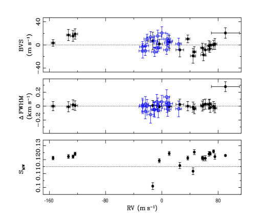
Figure 4: BVS, FWHM and S-index variations versus the FEROS (black filled circles) and CHIRON (blue open circles) velocities for HIP 67537 (upper, middle and lower panel, respectively.)

7 Astrometric upper mass limit

Motivated by previous works (Reffert & Quirrenbach REF11 (2011); Sahlmann et al. SAH11 (2011); Díaz et al. DIA12 (2012)), we used the improved version of the Hipparcos astrometric data (Van Leeuwen VAN07 (2007)), to measure the inclination angle of the orbital plane, and thus to derive the actual mass of HIP 67537 $b$. To do this, we employed the method described in Sahlmann et al. (SAH11 (2011)). Briefly, from the residuals of the Hipparcos abscissa, we reconstructed the abscissa values, and recomputed the astrometric solution, but this time solving for 7-parameters, i.e., the parallax ($\varpi$), celestial position ($\alpha^{\star}$, $\delta$), proper motion ($\mu_{\alpha^{\star}}$, $\mu_{\delta}$), the inclination angle ($i$) and the longitude of the ascending node ($\Omega$). Using this method, several exoplanet and BD candidates have recently been confirmed (e.g. Wilson et al. WIL16 (2016)). We note that we have tested our method using some of the systems presented in Sahlmann et al. (SAH11 (2011)) and Wilson et al. (WIL16 (2016)), for which we obtained nearly identical results. An extensive description of the method and validation on real data will be presented soon (Jones in preparation).
The Hipparcos astrometric dataset of HIP 67537 is comprised by a total of 105 measurements, after removing one outlier (at the $>$ 4 $\sigma$ level), with a mean uncertainty of 1.97 mas and covering 1164 days. The solution type is 5, meaning that no indication of significant acceleration in the proper motion is observed. Unfortunately, due to the low astrometric amplitude of the signal ($a\,$sin $i$ = 0.19 mas) and the long orbital period of HIP 67537 $b$, which exceeds by a factor of two the Hipparcos data timespan, no astrometric signal was detected. However, we can put an upper mass limit, corresponding to the minimum inclination angle that would be detectable in the Hipparcos data. To do this, we generated synthetic astrometric datasets, including the gravitational effect from the unseen companion, for a given inclination angle. We note that the smaller the inclination angle, the larger the astrometric signal, thus the easier its detection. We then used the same method described above, but this time using the synthetic datasets, instead of the original Hipparcos data. For each realization, we used the Keplerian parameters from the 1000 bootstrap Keplerian solutions. We also generated Gaussian distributed errors for the Hipparcos abscissa residuals and the $\Omega$ values were randomly choose. Then, for each solution, we applied the permutation test, in which the dates of the Hipparcos observations are fixed, while the corresponding abscissa residuals are randomly permuted. The significance of the solution is set by the fraction of the permuted solutions that yield $\chi^{2}$ values greater than the original solution. Figure 5 shows the significance of the synthetic orbit as a function of the inclination angle. It can be seen that the significance of the solution increases steeply with decreasing inclination angle. For this star, a significance of 98.7% is reached at $i$ = 2 deg, corresponding to a maximum mass for the companion of 0.33 M_⊙ , while it drops to $\sim$ 90% at $i\sim$ 3.5 deg. By assuming $i$ = 2 deg as the minimum inclination angle, the probability that HIP 67537 $b$ is actually a stellar object is $\lesssim$ 7 % (corresponding to 2 deg $\lesssim$ $i$ $\lesssim$ 8 deg).

Figure 5: Significance of the solution to the synthetic datasets as a function of the inclination angle.

8 Summary and discussion

In this work we present more than 6 years radial velocity variations of the evolved star HIP 67537. Based on the Keplerian fit to the observed RVs and also from the astrometric orbital inclination constraints presented in the previous sections, HIP 67537 $b$ is most likely a massive substellar companion, in the super-planet to brown dwarf mass regime. By assuming random orbital inclination angles and based in the upper mass limit of $\sim$ 0.3 M_⊙ (at the $\sim$ 99% significance level) , the probability that the HIP 67537 companion is stellar in nature is only $\sim$ 7%. Moreover, out of the 24 binary companions detected in our sample, only 6 of them are found interior to 5 AU. Interestingly, these 6 companions have minimum masses $\gtrsim$ 0.3 M_⊙ (see Bluhm et al. BLU16 (2016)). A similar result is also observed in solar-type binaries (Raghavan et al. RAG10 (2010)). In fact, hydrodynamical simulations show that close binary systems ($a\lesssim$ 10 AU) preferentially form with mass ratios close to unity (Bate et al. 2002). This means that very low-mass binary companions are rarely found in relatively close-in orbits, consistent with the substellar companion hypothesis.
Figure 6 shows the position of HIP 67537 $b$ in the semimajor axis versus minimum mass diagram. The red circles correspond to giant host stars, while the small black dots are solar-type parent stars. Clearly HIP 67537 $b$ is placed in a barely populated region of this diagram. In fact, apart from $\nu$ Oph $c$ (Quirrenbach et al. QUI11 (2011); Sato et al. SAT12 (2012)), this is the only known super-planet/BD candidate known to orbit a giant star at such large orbital distance. Given its projected mass and semimajor axis, this object is located in the edge of the BD desert, making HIP 67537 $b$ a rare object. After HIP 97233 b (Jones et al. 2015a ), this is the second BD candidate detected by our program orbiting interior to 5 AU. Considering two BDs in our sample comprised by 166 stars, we obtain a fraction of $f$ = 1.2${}^{+1.5}_{-0.4}$ %, higher than $f\sim$ 0.5 - 0.8% reported by other RV surveys targeting solar-type stars (Marcy & Butler MAR00 (2000); Vogt et al. VOG02 (2002); Wittenmyer et al. WIT09 (2009); Sahlmann et al. SAH11 (2011)). Interestingly, both stars have masses $\gtrsim$ 1.9 M_⊙ , providing further indications that BDs are more efficiently formed around more massive stars (Lovis & Mayor LOV07 (2007); Mitchell et al. MIT13 (2013)), which are formed in denser environments and thus have more massive protoplanetary disks (Andrews et al. AND13 (2013)). Moreover, if we restrict our sample to intermediate-mass stars (M_⋆$\gtrsim$ 1.5 M_⊙ ), then the fraction of BD companions with $a\lesssim$ 5 AU rises to $f$ = 1.6${}^{+2.0}_{-0.5}$ %. For comparison, Borgniet et al. (BOR16 (2016)) found no BD with orbital periods less than 1000 days, from a sample of 51 intermediate-mass A-F dwarf stars, which are the main-sequence progenitors of GK giants (although there is a big debate on this subject; see Johnson & Wright JOHN13 (2013) and references therein). This result is in agreement with our findings, since our two BD candidates have $P>$ 1000 days.
Interestingly, the parent stars of these BD candidates are metal-rich, therefore it is plausible that they formed via core-accretion. According to Mordasini et al. (MOR09 (2009)) planets in massive and metal-rich disks can be formed at starting position $\sim$ 4-7 AU and can accrete a significant amount of mass in-situ, becoming super-planets (or BDs) prior to the disk dissipation and opening a gap in the disk. Subsequently, they move inward via type II migration (Papaloizou & Lin PAP84 (1984)) to their final position at $a\gtrsim$ 2 AU. In addition, these two systems present high orbital eccentricities ($e$ $\sim$ 0.6), in contrast to most giant planets orbiting giant stars, which are typically found in nearly circular orbits ($e\lesssim$ 0.2; e.g. Jones et al. JON14b (2014)). In fact, these are the only substellar objects in our sample with eccentricities exceeding $\sim$ 0.2 (updated orbital solutions and new EXPRESS systems will be presented in a forthcoming paper). Ribas & Miralda-Escudé (RIB07 (2007)) studied the eccentricity distribution of planets detected via RVs around solar-type stars and they found that the most massive planets (M_p $\gtrsim$ 4 M_jup ) tend to have larger orbital eccentricities than less massive objects. This observational trend has been more recently confirmed by Desidera et al. (DES12 (2012)) and Adibekyan et al. (ADI13 (2013)). From a theoretical point of view, the high eccentricity observed in giant planets can be explained by planet-planet encounters, leading to eccentricity excitation and radial migration (e.g. Rasio & Ford RAS96 (1996); Raymond et al. RAY10 (2010)). Moreover, according to Ida et al. (IDA13 (2013)), massive giant planets could be formed in multi-planet systems in massive and metal-rich disks, with circular orbits, and due to the interaction with other planets in the system their eccentricities are excited. As a consequence, during these encounters, the less massive planets are either ejected or scattered to wider orbits ($\gtrsim$ 30 AU). In fact, multi-planet systems comprised by two or more giant planets are common among intermediate-mass giant stars (Jones et al. JON16 (2016)), while systems comprised by a BD and a giant planet appear to be absent. This could be the result of the ejection of a smaller giant planet by a BD in the system, like HIP 67537 $b$ and HIP 97233 $b$. The detection of outer giant planet companions using direct imaging might provide strong observational evidence of this scenario. Other mechanisms could be also responsible for the observed high eccentricities of these systems. For instance, the eccentricity of super planets and BDs can be excited by a distant companion, via the Kozai-Lidov effect (Kozai KOZ62 (1962); Lidov LID62 (1962); Holman et al. HOL97 (1997)). This mechanism probably affects many planetary systems, given the large fraction of stellar companions observed at different stellar mass, including intermediate-mass evolved stars (e.g. Bluhm et al. BLU16 (2016); Wittenmyer et al. WIT17 (2017)). Unfortunately, due to the very limited number of known close-in brown dwarf companions it is still very difficult to either favor or discard different formation and evolution models. The discovery of more of these systems are mandatory to really understand how these very massive planets form and how they interact with the disk and the rest of the bodies in it, as well as to study the formation efficiency as a function of the stellar mass.

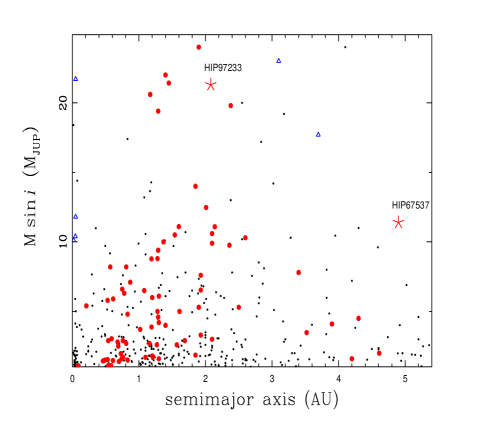
Figure 6: Minimum planet mass versus semimajor axis, for known giant planets (m_b sin$i$$\gtrsim$ 1.0 M_jup ). The black dots and red filled circles correspond to main-sequence and giant host stars. The blue open triangles are those systems with known inclination angles, thus they correspond to the true mass of the companion. The red asterisks show the position of HIP 67537 $b$ and HIP 97233 $b$.

Appendix A Radial velocity tables.

Table 2: Radial velocity variations of HIP 67537

JD - 2450000	RV	error	Instrument
	(m s-1 )	(m s-1 )
3072.8542	36.6	20.0	FEROS
5317.6184	29.5	2.9	FEROS
5379.6473	38.7	2.7	FEROS
5428.5237	51.8	3.8	FEROS
5729.6275	54.5	3.9	FEROS
5744.5979	68.0	2.9	FEROS
6047.6178	61.4	2.8	FEROS
6056.6058	60.7	3.3	FEROS
6066.6210	66.2	2.8	FEROS
6099.6025	59.7	3.1	FEROS
6110.5807	50.2	2.7	FEROS
6140.6110	37.0	3.8	FEROS
6321.7955	-140.3	2.8	FEROS
6331.8191	-133.8	3.9	FEROS
6342.7703	-131.0	3.8	FEROS
6412.6435	-162.3	2.7	FEROS
7072.8844	-20.5	6.6	FEROS
7388.8443	-11.1	4.2	FEROS
7471.9060	3.0	3.8	FEROS
7641.4875	18.2	5.5	FEROS
7012.8496	-17.5	4.2	CHIRON
7050.7982	-19.4	4.2	CHIRON
7079.7433	-12.8	4.4	CHIRON
7101.6655	1.0	4.8	CHIRON
7120.7170	-7.8	5.3	CHIRON
7140.7324	-19.0	5.3	CHIRON
7162.5652	-15.1	4.6	CHIRON
7181.4933	-2.2	4.4	CHIRON
7206.4763	-3.1	4.7	CHIRON
7255.4986	3.2	4.6	CHIRON
7260.4716	-15.3	5.2	CHIRON
7270.5026	16.5	4.7	CHIRON
7379.8748	15.0	4.3	CHIRON
7391.8555	8.2	5.6	CHIRON
7403.7968	2.3	5.5	CHIRON
7404.8142	15.8	5.0	CHIRON
7405.8539	18.2	5.4	CHIRON
7491.6450	32.1	4.2	CHIRON