Effective particles in quantum field theory

Abstract

The concept of effective particles is introduced in the Minkowski space-time Hamiltonians in quantum field theory using a new kind of the relativistic renormalization group procedure that does not integrate out high-energy modes but instead integrates out the large changes of invariant mass. The new procedure is explained using examples of known interactions. Some applications in phenomenology, including processes measurable in colliders, are briefly presented.

1 Introduction

Effective particles can be introduced in the quantum field theory (QFT) in such a way that their size plays the role of a scale parameter in a renormalization group procedure for the corresponding Hamiltonians. The example of QCD is particularly interesting because the effective quarks of large size are expected to correspond to the constituent quarks that are used in classification of hadrons, while point-like quarks and gluons correspond to partons used in description of hadrons in high-energy collisions. But the renormalization group procedure for effective particles (RGPEP) that is used here is not limited to QCD. Its general nature stems form the fact that one does not specify the size of quanta when one expands a quantum field in space into its Fourier modes. Namely, the Heisenberg and Pauli [1; 2] formulation of QFT is equally applicable to various particles despite the fact that they have different sizes, see Fig. 1. One can say that the concept of a quantum field operator is blind to the size of individual quanta. In contrast, in the renormalized theories derived using the RGPEP, this free size parameter determines the width of vertex form factors in the Hamiltonian interaction terms for effective particles.

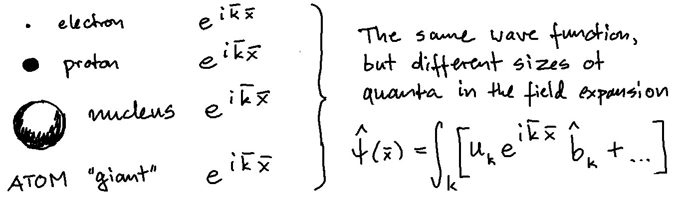
Figure 1: Quantum field operators are blind to the size of individual quanta.

2 Example of the RGPEP calculation: asymptotic freedom in Yang-Mills theory

Canonical quantization of the Yang-Mills (YM) theory begins with the Lagrangian density ${\cal L}=-\ {\rm tr}\,F^{\mu\nu}F_{\mu\nu}/2$, in which the field strength tensor is $F^{\mu\nu}=\partial^{\mu}A^{\nu}-\partial^{\nu}A^{\mu}+ig[A^{\mu},A^{\nu}]$. The associated energy-momentum tensor is ${\cal T}^{\mu\nu}=-F^{a\mu\alpha}\partial^{\nu}A^{a}_{\alpha}+g^{\mu\nu}F^{a\alpha\beta}F^{a}_{\alpha\beta}/4$. Consequently, the field four-momentum is given by $P^{\nu}=\int_{\Sigma}d\sigma_{\mu}\ {\cal T}^{\mu\nu}$, where $d\sigma_{\mu}$ is a measure on the hypersurface $\Sigma$ in the Minkowski space-time. In the front form (FF) of Hamiltonian dynamics [3], one uses the variables $x^{\pm}=t\pm z$ and $x^{\perp}=(x,y)$, with a similar convention for all tensors. The FF Hamiltonian results from integration of ${\cal H}_{YM}=T^{+\,-}$ over the front hypersurface $\Sigma$ defined by the condition $x^{+}=0$. The canonical FF Hamiltonian density in gauge $A^{+}=0$ contains three terms, ${\cal H}_{YM}={\cal H}_{A^{2}}+{\cal H}_{A^{3}}+{\cal H}_{A^{4}}$. Our example concerns the three-gluon term ${\cal H}_{A^{3}}$, to exhibit asymptotic freedom. Quantization is achieved by replacing the classical gauge-field $A$ by a field operator,

$$\quad\hat{A}^{\mu} = \sum_{k\sigma c}\left[t^{c}\,\varepsilon^{\mu}_{k\sigma}\,a_{k\sigma c}\,e^{-ikx}+t^{c}\,\varepsilon^{\mu*}_{k\sigma}\,a^{\dagger}_{k\sigma c}\,e^{ikx}\right]_{on~{}\Sigma}\ ,$$ (1)

where $a_{k\sigma c}$ and $a^{\dagger}_{k\sigma c}$ are the annihilation and creation operators of gluons with momentum $k=(k^{+},k^{\perp})$, polarization vectors $\varepsilon_{\sigma}$ and color matrices $t^{c}$ that span the algebra of $SU(N_{c})$. We consider the number of colors $N_{c}=3$. Thus, the starting Hamiltonian is

$$\hat{H}_{YM} = \int_{\Sigma}\ :{\cal H}_{YM}(\hat{A}):\ ,$$ (2)

where the double dots indicate normal ordering. Our focus is on the term that comes from ${\cal H}_{A^{3}}=g\ i\partial_{\alpha}A_{\beta}^{a}\ [A^{\alpha},A^{\beta}]^{a}$, which in the local quantum theory for point-like particles leads to

$$\hat{H}_{A^{3}} = \int_{x\,\in\,\Sigma}\ :g\ i\partial_{\alpha}\hat{A}_{\beta}^{a}(x)\ [\hat{A}^{\alpha}(x),\hat{A}^{\beta}(x)]^{a}:\ .$$ (3)

If the quanta are not point-like, see Fig. 2,

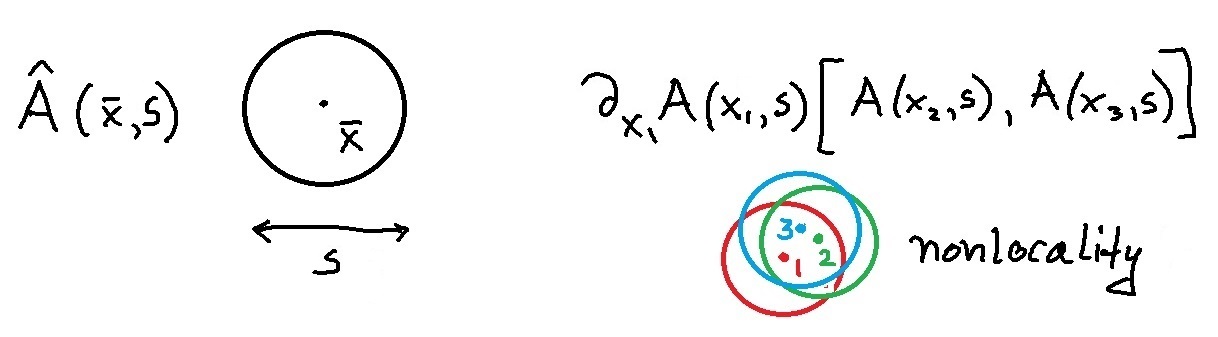
Figure 2: Nonlocal interaction of quanta of size $s$ can be approximated by a local interaction for wavelengths much greater than $s$. The effective particle size $s$ is the free scale parameter in the RGPEP.

the local interaction is merely an approximation, in which the size $s$ is a free parameter. Thus, instead of the quantum size-blind field operator $\hat{A}(x)$, we can introduce an effective particle quantum field $\hat{A}(x,s)$ and the non-local three-gluon interaction term

$$\hat{H}_{A^{3},s} = \int_{x_{i}\,\in\,\Sigma}\ g_{s}(x_{1},x_{2},x_{3})\ :i\partial_{\alpha}A_{\beta}^{a}(x_{1},s)\ [A^{\alpha}(x_{2},s),A^{\beta}(x_{3},s)]^{a}:\ .$$ (4)

The function $g_{s}(x_{1},x_{2},x_{3})$ is determined using the RGPEP, except that one works with momentum variables rather than the space-time coordinates. The required elements of the RGPEP can be found in a sequence of Refs. [4; 5; 6; 7; 8]. A brief summary of the procedure follows.

The RGPEP employs equations that connect theories with different values of the effective particle size $s$. There is an initial condition set at $s=0$ by canonical QCD. In our example,

$$\hat{H}_{A^{3},s=0} = \int_{x\,\in\,\Sigma}\ :g\ i\partial_{\alpha}\hat{A}_{\beta}^{a}(x,0)\ [\hat{A}^{\alpha}(x,0),\hat{A}^{\beta}(x,0)]^{a}:\ ,$$ (5)

where the field operator is built from creation and annihilation operators for point-like quanta,

$$\hat{A}^{\mu}(x,s=0) = \sum_{k\sigma c}\left[t^{c}\,\varepsilon^{\mu}_{k\sigma}\,a_{k\sigma c,s=0}\,e^{-ikx}+t^{c}\,\varepsilon^{\mu*}_{k\sigma}\,a^{\dagger}_{k\sigma c,s=0}\,e^{ikx}\right]_{on~{}\Sigma}\ .$$ (6)

Direct evaluation yields

$$\hat{H}_{A^{3},s=0} = \sum_{123}\ \delta_{12.3}\ \left[g\,Y_{123}\ a^{\dagger}_{1,0}\,a^{\dagger}_{2,0}\,a_{3,0}+g\,Y_{123}^{*}\ a^{\dagger}_{3,0}\,a_{2,0}\,a_{1,0}\right]\ ,$$ (7)

where an abbreviated notation is used, such as 1 in place of $k_{1},\sigma_{1},c_{1}$, the factor $\delta_{12.3}$ takes care of momentum conservation and the coefficients $Y_{123}$ stand for the gluon momentum, spin and color dependent factors implied by Eqs. (5) and (6). This is an example of a term in the general initial Hamiltonian for $s=0$. The general structure of the latter reads

$$H_{0}(a_{0}) = \sum_{n=2}^{\infty}\,\sum_{i_{1},i_{2},...,i_{n}}\,c_{0}(i_{1},...,i_{n})\,\,a^{\dagger}_{i_{1},0}\cdot\cdot\cdot a_{i_{n},0}\ ,$$ (8)

where the coefficients $c_{0}$ are determined by the regulated canonical theory and counterterms. In the same notation, the Hamiltonian for effective particles of size $s$ reads

$$H_{s}(a_{s}) = \sum_{n=2}^{\infty}\,\sum_{i_{1},i_{2},...,i_{n}}\,c_{s}(i_{1},...,i_{n})\,\,a^{\dagger}_{i_{1},s}\cdot\cdot\cdot a_{i_{n},s}\ ,$$ (9)

and the coefficients $c_{s}$ are calculated using the RGPEP. One of these coefficients is $g_{s}(i_{1},i_{2},i_{3})$ that corresponds to the function $g_{s}(x_{1},x_{2},x_{3})$ in Eq. (4).

The coefficients $c_{s}$ in Eq. (9) are derived from the condition that the Hamiltonian is not changed, $H_{s}(a_{s})=H_{0}(a_{0})$, when the canonical quanta with size $s=0$ are replaced by the effective quanta of size $s>0$, using a unitary transformation, $a_{s}=U_{s}\,a_{0}\,U_{s}^{\dagger}$. One works in a canonical operator basis and calculates the same coefficients $c_{s}$ using the operator ${\cal H}_{s}=H_{s}(a_{0})=U_{s}^{\dagger}H_{s}(a_{s})U_{s}$ that is determined by the RGPEP equations

$${\cal H}^{\prime}_{s} = \left[{\cal G}_{s},{\cal H}_{s}\right]\ ,$$ (10)

$${\cal G}_{s} = [{\cal H}_{f},\tilde{\cal H}_{s}]\ ,$$ (11)

where $\tilde{\cal H}_{s}$ differs from ${\cal H}_{s}$ only by multiplication of coefficients $c_{s}$ by the square of $+$-momentum carried by the corresponding product of creation or annihilation operators. This multiplication secures boost invariance of the effective theory. In Eqs. (10) and (11), the Hamiltonian is divided into a free part, equal to ${\cal H}_{0}$ for $g=0$, and the interaction ${\cal H}_{I}$, so that ${\cal H}_{s}={\cal H}_{f}+{\cal H}_{I}$. The key feature of solutions to these equations, and the reason for using them here, is that the coefficients $c_{s}$ exponentially suppress interactions that change the invariant mass of effective particles by more than $1/s$, see below. No modes are eliminated from the dynamics. Instead, vertex form factors suppress changes of invariant mass, see below.

Solutions to Eq. (10) define the YM theories a priori non-perturbatively. As such, they are not easy to obtain. In contrast, asymptotic freedom is found in the expansion in powers of the coupling constant,

$${\cal H}_{s} = {\cal H}_{f}+g{\cal H}_{1s}+g^{2}{\cal H}_{2s}+g^{3}{\cal H}_{3s}+...\ .$$ (12)

The terms of order $g$ and $g^{3}$ yield the result [8]

$$H_{A^{3}\,(1+3)s} = \sum_{123}\int_{123}\ \delta_{12.3}\ e^{-s^{4}\,{\cal M}_{12}^{4}}\ \left[\,V_{s123}\,a^{\dagger}_{1,s}a^{\dagger}_{2,s}a_{3,s}+V_{s123}^{*}\,a^{\dagger}_{3,s}a_{2,s}a_{1,s}\right]\ ,$$ (13)

in which ${\cal M}_{12}$ denotes the invariant mass of gluons 1 and 2. We see that the effective three-gluon interaction vertex is softened by the exponential form factor, which suppresses the interaction that involves a pair of gluons with invariant mass ${\cal M}_{12}$ the more the larger size $s$. The calculation shows that in the limit of vanishing relative transverse momentum of gluons $V_{s123}=g_{s}\ Y_{123}$ and

$$g_{s} = g_{0}+{g_{0}^{3}\over 48\pi^{2}}N_{c}\,11\,\ln{s\over s_{0}}\ .$$ (14)

The resulting Hamiltonian function $\beta(s)$ corresponds to the Green’s function $\beta(\lambda)$ obtained in Refs. [9; 10], where $\lambda$ denotes the length of a four-dimensional Euclidean momentum. Thus the effective particle formulation of QFT shows how the key feature of four-dimensional calculations of QCD manifests itself in the renormalized Hamiltonians. This way, the effective Hamiltonian approach passes an obligatory test for tackling issues of strong interaction theory. It provides the Minkowskian space-time scale parameter that corresponds to the abstract four-dimensional Euclidean scale parameter: the size of effective particles.

3 Early examples of RGPEP insight in phenomenology and theory of particles

The RGPEP provides a conceptual insight into particle dynamics in various systems. For example, in the case of protons, the universal RGPEP parameter $s$ tells us that the low-energy effective theory that can be sought using QCD, to support the quark model classification of hadrons, concerns quarks whose size is comparable with the size of the proton itself. Such large quarks ought to be thought about as built from partons of smaller size $s$, and the RGPEP provides mathematical tools for the corresponding construction of operators and states in the effective Fock-space basis. Using this insight, one can ask if the configurations of three bulky effective quarks built of small partons can explain ridge-like correlations in high-energy $pp$ collisions observed by the ATLAS and CMS collaborations at LHC [11; 12]. It was found [13] that among various simple models, including the gluon string stretched between a quark and a diquark [14], three quarks joined by a three-prong gluon body in the shape of letter Y, or a combination of various shapes and distributions of partons in effective particles, only the Y effective-particle picture of a proton provides eccentricity increasing with multiplicity. The model study [13] was carried out before the data exhibiting such type of behavior of $\sqrt{s}$ = 13 TeV $pp$ collisions [11; 12] were published. This example illustrates the phenomenological utility of the scale dependent, effective particle picture in QFT.

The RGPEP can be applied to QED in description of hydrogen and muonic hydrogen atoms [15] for the purpose of explanation of the difference between the proton radii extracted from data for level splittings in these atoms [16]. This is a computationally ambitious goal. But the question of principle that RGPEP answers is how to derive the Schrödinger equation from relativistic QFT. In QED, the RGPEP would start from the classical Lagrangian density ${\cal L}=-{1\over 4}F_{\mu\nu}F^{\mu\nu}+\bar{\psi}(i\partial/-eA/-m)\psi$. One treats the electrons and protons as point-like and proceeds to quantization as in Sec. 2 to obtain $\hat{H}$, regularize it, identify counterterms and calculate $\hat{H}_{QED\,s}$. The eigenvalue problem, $\hat{H}_{QED\,s}|\psi_{s}\rangle=E|\psi_{s}\rangle$ is identified with the Schrödinger equation for the hydrogen atoms represented as lepton-proton bound states when the size parameter $s$ is sufficiently large to prevent the interactions from inducing the invariant mass changes that exceed the constituent masses. The RGPEP valence constituent picture of atoms is illustrated schematically by

$$\left[\begin{array}[]{c}..\\ ..\\ e\gamma e\bar{e}p\gamma\\ e\gamma p\gamma\\ e\gamma p\\ \framebox{ $ep$ }\end{array}\right] = \left[\begin{array}[]{c}..\\ ..\\ e\gamma e\bar{e}\\ e\gamma\gamma\\ e\gamma\\ e\end{array}\right]\times\left[\begin{array}[]{c}..\\ ..\\ pe\bar{e}\\ p\gamma\gamma\\ p\gamma\\ p\end{array}\right]+...\,=\,|e_{s}p_{s}\rangle+...\ .$$ (33)

The left column represents a hydrogen atom as a superposition of virtual particle components in canonical theory, the size of quanta $s=0$. The lowest Fock component is put in a frame to indicate the state that provides the first approximation to an atom when one works with canonical QED. Once one introduces the effective quanta, the whole tower of Fock components is rewritten as an effective state of $|e_{s}p_{s}\rangle$ plus more effective-particle components, indicated by the three dots. When the size parameter $s$ is increased, the canonical interactions that act in and among all the Fock components are increasingly transformed into a complex interaction that predominantly acts in the component $|e_{s}p_{s}\rangle$, because the change of the number of quanta, even massless photons, involves much larger changes of invariant mass than the changes that occur in the component $|e_{s}p_{s}\rangle$. For sufficiently large $s$ and for small $\alpha$, the eigenvalue equation $\hat{H}_{QED\,s}|\psi_{s}\rangle=E|\psi_{s}\rangle$ can be reduced to the eigenvalue equation for the component $|e_{s}p_{s}\rangle$, which, after including proton electromagnetic form factors, especially the electric one, $G_{E}$, takes the familiar Schrödinger form up to terms of formal order $\alpha$,

$${\vec{p}\,^{2}\over 2\mu}\,\psi_{s}(\vec{p}\,)+\int{d^{3}k\over(2\pi)^{3}}\,V_{s}(\vec{p},\vec{k}\,)\,\psi_{s}(\vec{k}\,) = -E_{B}\,\psi_{s}(\vec{p}\,)\ ,$$ (34)

where the potential is

$$V_{s}(\vec{p},\vec{k}\,) = e^{-s^{4}(\vec{p}^{\,2}-\vec{k}^{\,2})^{2}/c^{4}}\ \ {-4\pi\alpha\over\vec{q}\,^{2}}\ \ G_{E}(\vec{q}\,^{2})\ .$$ (35)

The three-momentum transfer is $\vec{q}=\vec{p}-\vec{k}$. The exponential factor that corrects the Coulomb potential of extended proton, suppresses the interaction that changes the invariant mass of effective electron-proton system by more than $1/s$. Once the size $s$ is selected to secure universal scaling of atomic levels with $\alpha$, setting $s\sim 1/\sqrt{\mu M}$, where $\mu$ is the reduced and $M$ the average constituent mass, this factor introduces a small dependence of the potential on the lepton mass. This minuscule dependence has a divergent perturbative expansion in powers of $\alpha$ when one expresses momenta in units of $\alpha\mu c$. Therefore, it needs to be evaluated numerically. It turns out that it is capable of producing a lepton-mass correction in the extraction of proton radius from atomic levels, of the same magnitude [15] as the variation encountered in the proton radius puzzle [16] when the effective nature of particles appearing in the Schrödinger equation according the RGPEP is not accounted for.

It is worth pointing out that the Schrödinger equation emerges from the RGPEP derivation of effective low-energy Hamiltonian in QFT using the three-momentum variables $\vec{p}=(p^{\perp},p^{z})$,

$$p^{\perp} = c\ \left[(1-x)\ p_{l}^{\perp}-x\ p^{\perp}_{p}\right]/\sqrt{x(1-x)}\ ,$$ (36)

$$p^{z} = c\ (m_{l}+m_{p})\ (x-\beta)/\sqrt{x(1-x)}\ ,$$ (37)

where $\beta=m_{l}/(m_{p}+m_{l})$, $c=\sqrt{m_{l}m_{p}}/(m_{l}+m_{p})$, $x=p^{+}_{l}/(p^{+}_{l}+p^{+}_{p})$, while $l$ refers to lepton and $p$ to proton. These variables correspond to the relative momentum variables used in light-front holography [17] for description of hadrons. They appear to be non-relativistic while they are in fact the relative momenta of constituents in a relativistic theory, in which boost invariance is maintained. The correspondence is unlikely to be a meaningless coincidence. The Schrödinger equation is universally valid as an effective theory for atomic physics, despite that it apparently contains no remnants of complexity of relativistic QED. Similarly, the light-front holography [17], motivated by the idea of duality [18], is meant to approximate complex QFT in terms of solutions to relatively simple field equations in AdS [19]. In the case of strong interactions, the same variables are also used in showing that the linear confining potential in the instant form of dynamics [3] corresponds to a quadratic one in the FF [20].

4 Jet production in pion-nucleus collisions

When a pion with energy on the order of TeV collides with a platinum target, as in the E791 Fermilab experiment [21], and diffractively dissociates into two jets, the observed jet distribution is expected to report on the quark-antiquark pion wave function. The collision is illustrated in Fig 3.

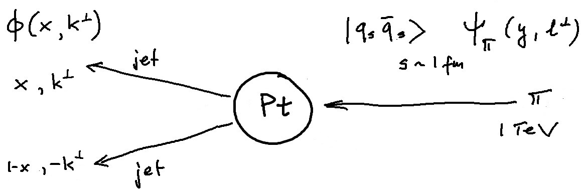
Figure 3: Pion is split into two quark jets on the gluons in a nucleus that act like a wedge.

Our description of it is based on Ref. [22].

One represents the incoming pion as a bound state of two quarks of constituent size $s_{c}$. According to Refs. [19; 20], the effective constituent wave function should be a solution of a holographic eigenvalue equation [17] with a quadratic effective potential, which for the ground state is Gaussian, $\psi_{\pi}\sim\exp{[-{\cal M}_{q\bar{q}}^{2}/(2\varkappa^{2})]}$ where the constituent invariant mass squared is ${\cal M}_{q\bar{q}}^{2}=(l^{\perp\,2}+m_{c}^{2})/[y(1-y)]=4(\vec{l}\,^{2}+m^{2}_{c})$. $\varkappa$ is a parameter of the quadratic effective potential written as $U_{\rm eff}=\varkappa^{4}r^{2}/4$ in terms of the relative distance $r$ between the quark and antiquark, canonically conjugated to the relative momentum variables of Eqs. (36) and (37) according to quantum mechanics. The quark carries fraction $y$ and antiquark fraction $1-y$ of the pion large $+$-momentum. The pion transverse momentum is zero, and the quark carries transverse momentum $l^{\perp}$ while the antiquark carries $-l^{\perp}$. The wave function is normalized to 1, assuming that the effective quarks of size $s_{c}$ saturate the pion state, as it should be the case according to the classification of hadrons in particle data tables [23]. The spin and isospin details are described by multiplying the Gaussian factor by $\bar{u}(p_{\pi}/\hskip 4.0pt+M)v$ [22]. The wave function parameters are adjusted to reproduce the pion radius and decay constant as well as the Gell-Mann–Okubo formula [24; 25]: $m_{c}\sim 331$ MeV, $\varkappa\sim$ 436 MeV and $M\sim-1.9$ GeV. The pion radius squared is $\sim 0.44$ fm² while data provide 0.45(1) fm² [23]. Weak decay constant is $f_{\pi}\sim$ 130.7 MeV, to be compared with the experimental value of 130.4 MeV [23]. The fitted value of $\varkappa$ is about 25% smaller than one could expect on the basis of other models [20]. The pion electromagnetic form factor obtained using these parameters is plotted in Fig. 4.

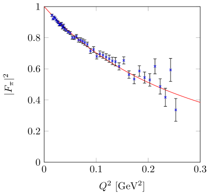
Figure 4: The pion electromagnetic form factor at low momentum transfers for the wave function model with holographic effective potential $U_{\rm eff}=\varkappa^{4}r^{2}/4$ in AdS/QCD [17; 20]. Data points are from Ref. [26].

When the high-energy pion hits the nucleus and its constituents interact with the target, the low-energy wave-function picture for the pion as built just from one constituent quark and one constituent

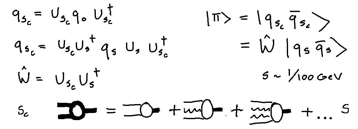
Figure 5: $|\pi\rangle=|q_{s_{c}}\bar{q}_{s_{c}}\rangle$ in terms of quarks and gluons with $1/s\sim 100$ GeV.

antiquark is not adequate. We need to express the quarks of size $s_{c}$ by the quarks and gluons of much smaller size $s$ for which we know the nuclear distribution. For example, to use the platinum distribution of gluons in the Bjorken variable $x$ for $Q\sim$ 100 GeV [27], we need to use the RGPEP operator $U_{s}$ to transform the quarks from scale $s_{c}$ to the quarks of scale $s\sim(100\rm GeV)^{-1}$. This is illustrated in Fig. 5. The required formula reads

$$|\pi\rangle = |q_{s_{c}}\bar{q}_{s_{c}}\rangle\,=\,\hat{W}_{s\,s_{c}}|q_{s}\bar{q}_{s}\rangle\ ,$$ (38)

where the state $|q_{s}\bar{q}_{s}\rangle$ has the same wave function as $|q_{s_{c}}\bar{q}_{s_{c}}\rangle$, $\hat{W}=U_{s_{c}}U^{\dagger}_{s}$ and both operators $U$ are expressed in terms of creators and annihilators of effective particles of size $s$. The operator $\hat{W}$ can be evaluated using expansion in powers of the coupling constant $g_{s}$, which is equivalent to expansion in powers of bare $g$ when one limits the calculation to terms order 1, $g$ and $g^{2}$. To this order, the pion quark-antiquark constituent state has components with quark-antiquark, quark-antiquark-gluon and quark-antiquark-gluon-gluon of the small size $s$. Thus, the calculation of splitting of a pion into two jets amounts to evaluation of action of $\hat{W}$ on the constituent model of pion suggested by AdS/QCD-based holography and calculating scattering amplitude of the resulting components into final quarks, whose momenta are identified with the momenta of the outgoing jets. Examples of the diagrams that contribute are provided in Fig. 6.

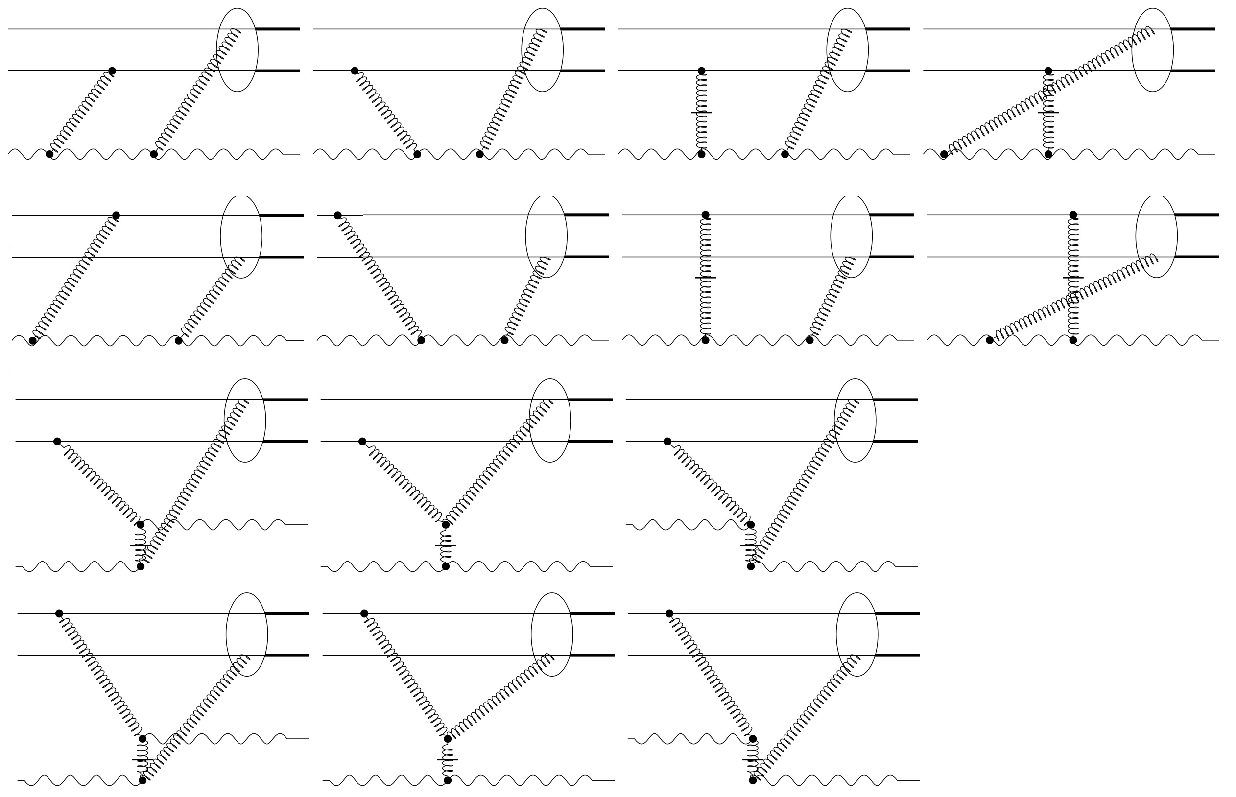
Figure 6: Examples of interactions that split the pion on gluons in a nucleus according to $H_{QCDs}$ with $1/s\sim 100$ GeV [22].

The resulting jet counts distributions, $\phi(x,k^{\perp})$ in Fig. 3, in comparison with data that are available in two bins of the jet $k^{\perp}$, are shown in Fig. 7. The absolute normalization factor for the theoretical curves is freely adjusted in both bins, the required coefficients in low to high $k^{\perp}$ bin being of ratio 13/11. The shapes of theoretical curves are in a reasonably good agreement with experimentally observed distributions of jets. However, the calculation does not include effects of propagation of leading quarks through the nucleus and misses description of hadronization. Inclusion of these elements requires development of the RGPEP beyond the current stage.

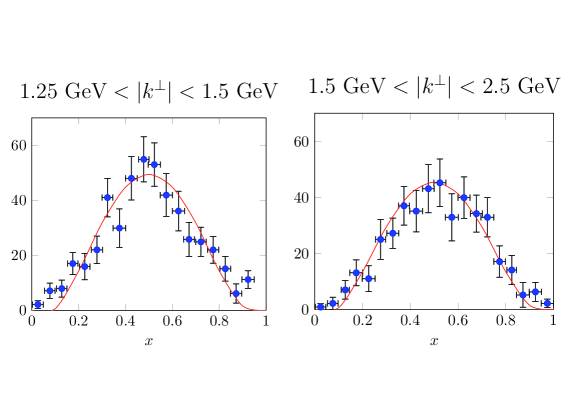
Figure 7: Jet counts distribution $\phi(x,k^{\perp})$, for jets induced by pions impinging on Pt, in two jet-$k^{\perp}$ bins; data points are from Ref. [21] and theory curves from Ref. [22].

5 Conclusion

The RGPEP opens new options for developing QFT and applying it in phenomenology of particle, nuclear and atomic physics. We are focused mainly on strong interactions. A critical step that awaits performing in QCD is to derive the Hamiltonian for effective particles with accuracy to fourth power of the coupling constant $g$. This Hamiltonian is expected to contain so far unknown terms whose structure may shed new light on the form of effective dynamics that applies to hadrons understood in terms of constituent quarks. The simplest theory to start with is QCD of quarks with masses much larger than $\Lambda_{QCD}$ in the RGPEP scheme. The goal would be to understand the dynamics of effective gluons in colorless objects, with the heavy quarks serving as anchors for the system. Extension to light quarks will require understanding of how many of them participate in the dynamics. This number will be determined by the ratio of $\Lambda_{QCD}$ to the light quark masses, which is on the order of 100. Such large number explains why the answer is not simple to obtain. It involves understanding of the Hamiltonian mechanism of breaking chiral symmetry and buildup of confinement. The RGPEP does not provide any ready answers to these questions, but it does offer tools for required studies. In particular, the effective coupling constant $g_{s}$ at suitable values of quark and gluon size $s$ is not known yet and, so far, we do not have any theoretical estimates for the probability of finding large numbers of light quarks in eigenstates of $\hat{H}_{QCD\,s}$ with any value of $s$ that is likely to be effective in describing light hadrons.