An extended Perona-Malik model based on probabilistic models

Abstract

The Perona-Malik model has been very successful at restoring images from noisy input. In this paper, we reinterpret the Perona-Malik model in the language of Gaussian scale mixtures and derive some extensions of the model. Specifically, we show that the expectation-maximization (EM) algorithm applied to Gaussian scale mixtures leads to the lagged-diffusivity algorithm for computing stationary points of the Perona-Malik diffusion equations. Moreover, we show how mean field approximations to these Gaussian scale mixtures lead to a modification of the lagged-diffusivity algorithm that better captures the uncertainties in the restoration. Since this modification can be hard to compute in practice we propose relaxations to the mean field objective to make the algorithm computationally feasible. Our numerical experiments show that this modified lagged-diffusivity algorithm often performs better at restoring textured areas and fuzzy edges than the unmodified algorithm. As a second application of the Gaussian scale mixture framework, we show how an efficient sampling procedure can be obtained for the probabilistic model, making the computation of the conditional mean and other expectations algorithmically feasible. Again, the resulting algorithm has a strong resemblance to the lagged-diffusivity algorithm. Finally, we show that a probabilistic version of the Mumford-Shah segementation model can be obtained in the same framework with a discrete edge-prior.

1 Introduction

In mathematical image processing, one is often given some (linear) forward operator $A:X\to Y$ and some noisy observation $v_{n}$. Our goal is to reconstruct a noise-free image that explains the observed data well, i.e. an approximate solution $u$ to $Au\approx v_{n}$. For example, $A$ can denote a convolution operator and $v_{n}$ a noisy measurement of the resulting blurry image.

Several approaches exist to solve problems of this type. One popular approach is via variational regularization scherzer2009variational ; bertero1998inverseproblems where one formulates a minimization problem and seeks the solution as a minimizer of a weighted sum of data fit (or discrepancy) term and a regularization term. The weighting factor is called regularization parameter and controls the trade-off between data fit and regularization. A related approach is to reconstruct $u$ via the solution of an appropriate partial differential equation. One of the earliest such partial differential equation is used in the Perona-Malik diffusion algorithm perona1990scalespace ; nordstrom1990biased ; weickert1998anisotropic where one solves the image reconstruction problem by computing stationary points of the nonlinear diffusion problem

$$\partial_{t}u+\tfrac{1}{\sigma^{2}}A^{\prime}(Au-v_{n})=\nabla\cdot\left(f\left(\frac{1}{2}|\nabla u|^{2}\right)\nabla u\right)$$ (1)

where $\sigma$ is an estimate for the noise level and $f:\mathbb{R}\to\mathbb{R}$ is some nonlinear, positive and decreasing function that stops the diffusion at points where $|\nabla u(x)|$ is large. In fact, the two approaches are closely related since the stationary points of this equation are indeed stationary points of the optimization problem

$$\min_{u}\frac{1}{2\sigma^{2}}\|Au-v_{n}\|^{2}+\int F\left(\frac{1}{2}|\nabla u(x)|^{2}\right)\mathrm{d}x,$$ (2)

where $F$ is any function with $F^{\prime}=f$.

An alternative approach is given by Bayesian statistics, where we define a prior distribution $p(u)$ on the space of possible images and model the forward model including the noise by the likelihood term $p(v_{n}\mid u)$. The posterior distribution is then given by

$$p(u\mid v_{n})=\frac{p(u)p(v_{n}\mid u)}{\int p(u)p(v_{n}\mid u)\mathrm{d}u}.$$ (3)

In theory, the posterior distribution carries all information that we put into the model but as a distribution on the space of all possible images it is very high dimensional and it is not straightforward to extract useful information. One piece of information is the so-called maximum-a-posterior (MAP) estimate which is simply the image $u$ that maximizes the posterior, i.e. the solution of

$$\max_{u}p(u)p(v_{n}\mid u)$$ (4)

which, by taking the negative logarithm, again amounts to a minimization problems. Beyond the MAP estimate there are other quantities that can be computed from the posterior distribution, see e.g. kaipio2005statistical for further information.

In this work we derive a probabilistic model for the image reconstruction problem and analyze different methods to extract information for the reconstruction. We show that using the expectation-maximization algorithm dempster1977maximum reproduces the lagged-diffusivity approach for the Perona-Malik equation vogel1996iterative ; chan1999convergence . However, other methods exists and in this work we specifically analyze a mean-field approach and a sampling strategy which lead to different methods that extend the Perona-Malik model.

Some advantages of the probabilistic approach to the image reconstruction problem are that uncertainty in the reconstruction is explicitly part of the model which can lead to more meaningful reconstructions. Moreover, estimates for the uncertainty can be computed, e.g. marginal variances. Also, the probabilistic model comes from a sound foundation that combines well with learning approaches in which parts of the reconstruction model itself are learned from the data as in chen2015learning . As a result, the probabilistic approach opens the full toolbox of Bayesian statistics and allows to employ further techniques, e.g. from the field of model selection yu2010imagemodelselection .

Probabilistic models have been used in image processing since long ago and we only give a few pointers. Geman and Geman geman1984stochastic were one of the first to propose a probabilistic framework for image restoration tasks. They use simulated annealing for optimization, which is often not very efficient. More recently, and closer to our work, Schmidt et al. schmidt2010agenerative use Gaussian scale mixtures to train generative image models for denoising and inpainting tasks. A classical resource for the statistical treatment of inverse problems is given in kaipio2005statistical . Other probabilistic approaches to the Perona-Malik model differ from our approach: On the one hand krim1999nonlinear ; bao2004smart build on stochastic partial differential equations and random walks on lattices and not on Bayesian statistics. On the other hand pizurica2006bayesian takes a Bayesian approach to non-linear diffusion but derives a new diffusivity function $f$ by these means.

The article is organized as follows. In Section 2 we introduce our model based on Gaussian scale mixtures, introduce the notion of an exponential pair of random variables and derive a few properties of our model. Section 3 gives three methods to infer information from the posterior distribution, namely expectation-maximization, mean field methods and sampling. In Section 4 we present results of our methods and in Section 5 we draw some conclusions.

2 Gaussian Scale Mixtures

In the following we denote by $\Omega$ the domain of the image which we assume to be a regular rectangular grid, by $x\in\Omega$ the pixels and by $u$ the image, i.e $u(x)\in\mathbf{R}$ is the gray value of $u$ at pixel $x$. We denote by $\nabla u(x)\in\mathbf{R}^{2}$ the discrete gradient of $u$ at $x$, i.e.

$$\nabla u(x_{1},x_{2}):=\begin{pmatrix}u(x_{1}+1,x_{2})-u(x_{1},x_{2})\\ u(x_{1},x_{2}+1)-u(x_{1},x_{2})\end{pmatrix}.$$

For a vector field $v:\Omega\to\mathbf{R}^{2}$ we denote by $\nabla\cdot v(x)$ the discrete divergence of $v$ at $x$, i.e.

$$\nabla\cdot v(x_{1},x_{2}):=v_{1}(x_{1},x_{2})-v_{1}(x_{1}-1,x_{2})\\ +v_{2}(x_{1},x_{2})-v_{2}(x_{1},x_{2}-1).$$

Moreover, boundary conditions are chosen such that $\nabla$ and $-\nabla\cdot$ are adjoint to each other.

A Gaussian model for the magnitude of the gradient of $u$ corresponds to a density

$$p(u)\propto\exp\Big{(}-\tfrac{\lambda}{2}\sum_{x\in\Omega}|\nabla u(x)|^{2}\Big{)}.$$

If we further assume that our observation $v_{n}$ is obtained by $Au$ plus Gaussian white noise with variance $\sigma^{2}$, the corresponding likelihood is also Gaussian

$$p(v_{n}\mid u)\propto\exp\Big{(}-\tfrac{1}{2\sigma^{2}}\|Au-v_{n}\|^{2}\Big{)}.$$

Consequently, the posterior density is given by

$$p(u\mid v_{n})\propto\exp\big{(}-\tfrac{1}{2\sigma^{2}}\|Au-v_{n}\|^{2}-\tfrac{\lambda}{2}\sum_{x\in\Omega}|\nabla u(x)|^{2}\big{)}.$$

It is well known, that this model is not well-suited to denoise or deblur natural images, e.g. one observes that the MAP estimate for $u$ cannot have sharp edges anymore.

We propose a Gaussian scale mixture (GSM) for the magnitude of the gradient, that is a Gaussian model with additional latent scale variables $z(x)$, i.e. prior models that have a density of the form

$$p(u,z)\propto\exp\left(-\sum_{x}\left(\frac{z(x)}{2}|\nabla u(x)|^{2}+v(z(x))\right)\right)$$ (5)

with respect to some reference measure $\lambda^{n}(\mathrm{d}u)\otimes\bigotimes_{x}q(\mathrm{d}z(x))$. Here, $\lambda^{N}$ denotes the $N$-dimensional Lebesgue measure and $q$ is a $1$-dimensional Borel measure on $[0,\infty)$, for example the Lebesgue measure on $[0,\infty)$ or the counting measure on some discrete subset of $[0,\infty)$.

Intuitively, the introduction of such latent scales allows the model to freely “choose” the $z(x)$ in the most appropriate way. In particular, the model can “choose” to make the $z(x)$ small on edges, if this increases the overall probability. When done right, this can fix the inability of the Gaussian model to preserve edges.

Given a noisy measurement $v_{n}$ of $Au$ with Gaussian noise, the posterior density $p(u,z\mid v_{n})$ is given by

$$p(u,z\mid v_{n})\propto\exp\Bigl{(}-\frac{1}{2\sigma^{2}}\|Au-v_{n}\|^{2}\\ -\frac{1}{2}\sum_{x}z(x)|\nabla u(x)|^{2}-\sum_{x}v(z(x))\Bigr{)}.$$ (6)

Let

$$\mu(\mathrm{d}u)=\lambda^{n}(\mathrm{d}u)\quad\text{and}\quad\nu(\mathrm{d}z)=\bigotimes_{x\in\Omega}q(\mathrm{d}z(x)).$$

The density in (6) with respect to $\mu\otimes\nu$ is of the form

$$p(u,z\mid v_{n})\propto\exp\left(\langle s_{0}(u),r_{0}(z)\rangle+h(u)+g(z)\right)$$ (7)

with so-called sufficient statistics

$$s_{0}(u)=\left(-\frac{1}{2}|\nabla u(x)|^{2}\right)_{x\in\Omega}\quad\text{and}\quad r_{0}(z)=z$$ (8)

and

$$h(u)=-\frac{1}{2\sigma^{2}}\|Au-v_{n}\|^{2}\quad\text{and}\quad g(z)=-\sum_{x}v(z(x)).$$ (9)

We call a pair of random variables $(u,z)$ that has a density of the form (7) with respect to some reference measure $\mu\otimes\nu$ an exponential pair of random variables. The name exponential pair is inspired by the fact that any exponential pair, both conditional densities $p(u\mid z,v_{n})$ and $p(z\mid u,v_{n})$ are in the exponential family, i.e. they are of the form $x\mapsto\mathrm{e}^{\theta^{\intercal}\bar{s}(x)-\bar{A}(\theta)}$, see (murphy2012machine, , Section 9.2) for details. Using $s=(s_{0},h,1)$ and $r=(r_{0},1,g)$, the density of an exponential pair with respect to $\mu\otimes\nu$ can also be written in the form

$$p(u,z\mid v_{n})\propto\exp\left(\langle s(u),r(z)\rangle\right).$$ (10)

We will use the notion of an exponential pair later in Section 3.2 to derive mean field approximations.

To see how the GSM in (6) is related to the Perona-Malik model, we introduce

$$\psi(t)=-\log\int\mathrm{e}^{-tz-v(z)}q(\mathrm{d}z).$$ (11)

and marginalize out the $z(x)$ in (6): A simple calculation shows that

$$\int\exp\Big{(}\sum_{x}-\tfrac{1}{2}z(x)|\nabla u(x)|^{2}-v(z(x))\Big{)}q(dz)\\ =\prod_{x}\int\exp\Big{(}-\tfrac{1}{2}z(x)|\nabla u(x)|^{2}-v(z(x))\Big{)}q(dz(x))\\ =\prod_{x}\exp(-\psi(\tfrac{1}{2}|\nabla u(x)|^{2})\Big{)}\\ =\exp\Big{(}-\sum_{x}\psi(\tfrac{1}{2}|\nabla u(x)|^{2})\Big{)}$$

and we obtain

$$p(u\mid v_{n})\propto\exp\Biggl{(}-\frac{1}{2\sigma^{2}}\|Au-v_{n}\|^{2}\\ -\sum_{x}\psi\left(\frac{1}{2}|\nabla u(x)|^{2}\right)\Bigr{)}.$$ (12)

We see that the squared magnitude of the gradient is no longer penalized linearly, but rescaled according to $\psi$ which is precisely the variational formulation (2) of the Perona-Malik model.

In what follows, the derivatives of $\psi$ will play an important role. The following lemma is an easy consequence of an analogous result from the theory of exponential families:

Lemma 1

$\psi$ is smooth on $(0,\infty)$ with first and second derivative

1. $\psi^{\prime}(t)=\operatorname{E}\left(z(x)\mid\frac{1}{2}|\nabla u(x)|^{2}=t\right)$

2. $\psi^{\prime\prime}(t)=-\operatorname{Var}\left(z(x)\mid\frac{1}{2}|\nabla u(x)|^{2}=t\right)$.

In particular, $\psi$ is a concave function.

Proof

By logarithmic differentiation and looking at (5), we calculate the derivative of $\psi$ as

$$\psi^{\prime}(t) =\frac{\int z\mathrm{e}^{-tz-v(z)}q(\mathrm{d}z)}{\int\mathrm{e}^{-tz-v(z)}q(\mathrm{d}z)}$$

$$=\operatorname{E}\left(z(x)\;\Big{|}\;\frac{1}{2}|\nabla u(x)|^{2}=t\right).$$

For the second claim note that (using 1.)

$$\operatorname{Var}\left(z(x)\mid\frac{1}{2}|\nabla u(x)|^{2}=t\right)\\ =\operatorname{E}\left(z(x)^{2}\;\Big{|}\;\frac{1}{2}|\nabla u(x)|^{2}=t\right)-\psi^{\prime}(t)^{2}$$

which, after some manipulation, evaluates to $-\psi^{\prime\prime}(t)$.∎

The fact that $\psi$ is a concave function has the important consequence that computing a MAP-assignment of (12) generally leads to non-convex optimization problems.

Moreover, Lemma 1 implies that we can compute the first and second order moments of $z$ given $u$ without having an explicit representation of the joint distribution $p(u,z)$. All we need is an explicit representation of $\psi$ and knowledge that such an explicit representation exists. Note that the function $\Psi(t)=\mathrm{e}^{-\psi(t)}$ is in fact the Laplace transform of the measure $\mathrm{e}^{-v}q$. By Bernstein’s theorem, we know that $\psi$ can be written in the form (11) if an only if $\Psi(t)=\mathrm{e}^{-\psi(t)}$ defines a completely monotone function andrews1974scale , i.e. for $k\geq 0$ it holds that $(-1)^{k}\Psi^{(k)}\geq 0$.

Using the particularly simple $v(z)=z$ and $q$ being the Lebesgue measure on $(0,\infty)$ we get

$$\psi(t)=-\log\int_{0}^{\infty}e^{-tz-z}dz=-\log\left(\frac{1}{1+t}\right)=\log(1+t).$$

Using this $\psi$ in (12) we obtain the respective minimization problem (2) with $F=\psi$ and hence, the differential equation (1) is

$$\partial_{t}u+A^{\prime}(Au-u_{n}) =\nabla\cdot\Big{(}\psi^{\prime}\big{(}\tfrac{1}{2}|\nabla u|^{2}\big{)}\nabla u\Big{)}$$

$$=\nabla\cdot\Bigg{(}\frac{\nabla u}{1+\tfrac{1}{2}|\nabla u|^{2}}\Bigg{)}$$

which is the original Perona-Malik model perona1990scalespace . Note that Lemma 1 provides a new interpretation for the diffusion coefficient: it says that the diffusion coefficient $\psi^{\prime}$ is the expectation of the latent variable $z$ conditioned on the current magnitude of the image gradient. The other proposed function from perona1990scalespace , $\psi^{\prime}(t)=\exp(-t)$ leads to $\psi(t)=1-\exp(-t)$. This function also fits into our framework, since the mapping $\Psi(t)=\exp(-\psi(t))=\exp(\exp(-t)-1)$ can be shown to be completely monotone. However, we are not aware of a closed form for the inverse Laplace transform of this function, and hence, the form of $v$ remains elusive in this case.

3 Methods

In this section we develop different approaches to use the posterior density (6) for image reconstruction tasks, such as denoising or deblurring.

3.1 MAP estimation

The first method we derive solves the maximum a-posteriori (MAP) problem for Gaussian scale mixtures like in (5), i.e. we consider the posterior distribution over $u$ and $z$, which is given by

$$p(u,z\mid v_{n})\propto\exp\Bigl{(}-\frac{1}{2\sigma^{2}}\|Au-v_{n}\|^{2}\\ -\sum_{x}\left(\frac{1}{2}z(x)|\nabla u(x)|^{2}+v(z(x))\right)\Bigr{)}$$ (13)

and aim for a maximizer of the distribution.

As derived in the previous section, the marginal distribution with respect to $u$ is

$$p(u\mid v_{n})\propto\exp\Biggl{(}-\frac{1}{2\sigma^{2}}\|Au-v_{n}\|^{2}\\ -\sum_{x}\psi\Bigl{(}\frac{1}{2}|\nabla u(x)|^{2}\Bigr{)}\Biggr{)}.$$ (14)

There are two different versions of MAP-assignments that can be computed: we can either compute the MAP of both $u$ and $z$ with respect to the joint distribution $p(u,z\mid v_{n})$ or the MAP of either $u$ or $z$ with respect to the marginal distributions $p(u\mid v_{n})$ and $p(z\mid v_{n})$.

Both methods can be understood as methods of approximating the joint distribution $p(u,z\mid v_{n})$ by a simpler, possibly deterministic, probability distribution. However, computing the MAP over the joint distribution is generally a crude approximation, as it approximates $p(u,z\mid v_{n})$ with a completely deterministic distribution. In contrast to this, computing the MAP with respect to $p(u\mid v_{n})$ still captures the uncertainty in $z$. An even better alternative is to use mean field approximations which we will discuss in Section 3.2.

In this paper we consider the problem of computing a MAP-assignment with respect to the marginal model in (14). The corresponding optimization problem can be written as

$$\min_{u}\frac{1}{2\sigma^{2}}\|Au-v_{n}\|^{2}+\sum_{x}\psi\left(\frac{1}{2}|\nabla u(x)|^{2}\right).$$ (15)

In general, there are multiple optimization methods that can be employed and in some cases there are specialized methods to solve the optimization problem. For example, if $t\mapsto\psi\left(t^{2}\right)$ defines a convex function, we can use tools from convex optimization to solve the optimization problem. However, this is not the case for general $\psi$, so that it makes sense to look for general purpose algorithms.

A simple option is to use gradient descent on (15) which formally leads to the iteration

$$u^{k+1}=u^{k}\\ -h_{k}\Big{(}\tfrac{1}{\sigma^{2}}A^{\prime}(Au^{k}-v_{n})-\nabla\cdot\big{(}\psi^{\prime}(\tfrac{1}{2}|\nabla u^{k}|^{2})\nabla u^{k})\big{)}\Big{)}.$$

For suitable stepsizes $h_{k}$ this is a descent method, but the choice of stepsize is cumbersome and convergence is usually slow. A second option is to use EM as we describe later in this section. Before we do so, we would like to describe another way: As $-\psi$ is a convex function (which we extend by $+\infty$ for negative arguments), it is also possible to dualize $-\psi$ as

$$-\psi(t)=\max_{s\in\mathbb{R}}\Big{\{}s\,t-(-\psi)^{*}(s)\Big{\}}$$

which we also write as

$$\psi(t)=\min_{s\in\mathbb{R}}\Big{\{}-s\,t+(-\psi)^{*}(s)\Big{\}}.$$

Hence, we can reformulate (15) as

$$\min_{u,s}\frac{1}{2\sigma^{2}}\|Au-v_{n}\|^{2}+\sum_{x}\left(-s(x)\tfrac{1}{2}|\nabla u(x)|^{2}\right.\\ +\left.(-\psi)^{*}\left(s(x)\right)\right).$$

Since the problem is convex in both $u$ and $s$ (but not jointly so), we can perform coordinate descent. This leads to the following updates:

$$s^{k+1} =-\psi^{\prime}(\tfrac{1}{2}|\nabla u^{k}|^{2})$$

$$u^{k+1} \leftarrow\text{solve}\ \tfrac{1}{\sigma^{2}}A^{\prime}(Au-v_{n})+\nabla\cdot(s^{k+1}\nabla u)=0$$

Here we used that the inverse of the derivative of $(-\psi)^{*}$ is $(-\psi)^{\prime}$. We can combine this into one iteration and get that $u^{k+1}$ is given as the solution of the linear equation

$$\tfrac{1}{\sigma^{2}}A^{\prime}(Au^{k+1}-v_{n})-\nabla\cdot(\psi^{\prime}(\tfrac{1}{2}|\nabla u^{k}|^{2})\nabla u^{k+1})=0.$$

In the context of the Perona-Malik equation, this scheme is known as lagged diffusivity vogel1996iterative ; chan1999convergence . From the above derivation we obtain a new proof of that fact that this scheme is indeed a descent method for the objective function in (15).

Next we derive an EM method and we will see that EM and the coordinate descent method are equivalent.

The EM method alternates between an E step (expectation) and an M step (maximization). In this particular example, we alternatingly estimate the $z$-variable and maximize with respect to the $u$ variable. The E step for $z$ is, as derived in Lemma 1

$$\xi_{0}^{(k)}\leftarrow\operatorname{E}(z(x)\mid\tfrac{1}{2}|\nabla u^{(k)}(x)|^{2})=\psi^{\prime}(\tfrac{1}{2}|\nabla u^{(k)}(x)|^{2})$$

and the M step is to maximize the expectation

$$\operatorname{E}_{z}\left(\log p(u,z\mid v_{n})\mid u^{(k)}\right)$$

with respect to $u$.

Together, this leads the scheme in Algorithm 1.

1:procedure gsm_map($v_{n}$)

2:     while not converged do

3:         for $x\in\Omega$ do

4:              $\xi_{0}(x)\leftarrow\psi^{\prime}(\tfrac{1}{2}|\nabla u(x)|^{2})$

5:         end for

6:         $u\leftarrow\operatorname{argmin}_{u^{\prime}}\frac{1}{2\sigma^{2}}\|Au^{\prime}-v_{n}\|^{2}+\frac{1}{2}\sum_{x}\xi_{0}(x)|\nabla u^{\prime}(x)|^{2}$

7:     end while

8:     return $u$

9:end procedure

Algorithm 1 EM algorithm for Gaussian scale mixture

On the other hand, the gradient of the objective function in (15) is given by

$$\frac{1}{\sigma^{2}}A^{\prime}(Au-v_{n})-\nabla\cdot\left(\psi^{\prime}\left(\frac{1}{2}|\nabla u|^{2}\right)\nabla u\right)$$

and gradient descent corresponds to solving the gradient flow

$$\partial_{t}u+\frac{1}{\sigma^{2}}A^{\prime}(Au-v_{n})=\nabla\cdot\left(\psi^{\prime}\left(\frac{1}{2}|\nabla u|^{2}\right)\nabla u\right).$$

Instead of finding stationary points of this equation by integrating the differential equation, this can be done more efficiently by using lagged diffusivity vogel1996iterative ; chan1999convergence , which we described above. If we set

$$\xi_{0}^{(k)}:=\psi^{\prime}\left(\frac{1}{2}|\nabla u^{(k)}|^{2}\right)$$ (16)

we have to solve the linear equation

$$\frac{1}{\sigma^{2}}A^{\prime}(Au-v_{n})-\nabla\cdot\left(\xi_{0}^{(k)}\nabla u\right)=0$$ (17)

for $u$ to obtain the next iterate $u^{(k+1)}$. As it turns out, for Gaussian scale mixtures, this is equivalent to EM:

Lemma 2

For Gaussian scale mixture models as in (5), EM and lagged diffusivity yield the same algorithm.

Proof

By Lemma 1, the updates of $\xi_{0}^{(k)}$ can be expressed as

$$\xi_{0}^{(k)}=\psi^{\prime}\left(\frac{1}{2}|\nabla u^{(k)}|^{2}\right)=\operatorname{E}(z\mid u^{(k)}).$$

Moreover, solving (17) is equivalent to minimizing

$$\frac{1}{2\sigma^{2}}\|Au-v_{n}\|^{2}+\frac{1}{2}\sum_{x}\xi_{0}^{(k)}(x)|\nabla u(x)|^{2}$$

with respect to $u$. Overall, we obtain $u^{(k+1)}$ from $u^{(k)}$ by minimizing

$$\frac{1}{2\sigma^{2}}\|Au-v_{n}\|^{2}+\frac{1}{2}\sum_{x}\operatorname{E}(z(x)\mid u^{(k)})|\nabla u(x)|^{2}$$

with respect to $u$, which is just the EM algorithm.∎

Lemma 2 implies that we can apply the convergence theory for EM to the lagged-diffusivity algorithm and vice versa.

3.2 Mean field approximations

MAP-assignments often yield non-representative samples of the posterior distribution kaipio2005statistical . A better alternative is given by mean field theory. Moreover, mean field approximation are often a good compromise between MAP-assignments that neglect uncertainties in the model and the conditional mean that can be problematic in a multimodal setting.

In this section, we describe how mean field theory can be applied to Gaussian scale mixtures.

The idea is to approximate the complicated distribution $p(u,z\mid v_{n})$ by a factorized distribution $q_{1}(u)q_{2}(z)$ as good as possible in some sense. The mean field approximation defines this sense as nearness in the Kullback-Leibler divergence. Hence, we denote with $p$ the density $p(u,z\mid v_{n})$ and seek distributions $q_{1}$ and $q_{2}$ such that

$$\operatorname{KL}(q_{1}q_{2},p)=\iint q_{1}(u)q_{2}(z)\log\left(\frac{q_{1}(u)q_{2}(z)}{p(u,z|v_{n})}\right)\mathrm{d}u\mathrm{d}z$$

is minimized. We rewrite this term with the help of the entropy $\mathbb{H}(q)=-\int q\log q=-\operatorname{E}(\log(q))$ as

$$\operatorname{KL}(q_{1}q_{2},p)=-\langle q_{1}q_{2},\log p\rangle-\mathbb{H}(q_{1})-\mathbb{H}(q_{2}).$$

Performing the minimization only over probability distributions $q_{1}$, we see that

$$\int\log(p(u,z|v_{n}))q_{2}(z)\mathrm{d}z-\log(q_{1}(u))=\operatorname{const}$$

and for $q_{2}$ we get

$$\int\log(p(u,z|v_{n}))q_{1}(u)\mathrm{d}u-\log(q_{2}(z))=\operatorname{const}.$$

Hence, we see, that alternating minimization for $q_{1}$ and $q_{2}$ leads to the updates

$$q_{1}^{(k+1)}(u) \propto\exp\Bigl{(}\int\log(p(u,z|v_{n}))q_{2}^{(k)}(z)\mathrm{d}z\Bigr{)}$$ (18)

$$=\exp\left(\operatorname{E}_{q_{2}^{(k)}(z)}(\log p(u,z|v_{n}))\right)$$

$$q_{2}^{(k+1)}(z) \propto\exp\Bigl{(}\int\log(p(u,z|v_{n}))q_{1}^{(k+1)}(u)\mathrm{d}u\Bigr{)}$$ (19)

$$=\exp\left(\operatorname{E}_{q_{1}^{(k+1)}(u)}(\log p(u,z|v_{n}))\right).$$

Note the resemblance of this procedure to the EM-algorithm. In contrast to the EM-algorithm, however, the mean field algorithm treats both $u$ and $z$ symmetrically and incorporates the uncertainty in both of them. The EM-algorithm ignores the uncertainty in $u$.

For Gaussian scale mixtures of the form (6) we have

$$\log p(u,z|v_{n})=-\frac{1}{2\sigma^{2}}\|Au-v_{n}\|^{2}\\ -\sum_{x}\left(\frac{1}{2}z(x)|\nabla u(x)|^{2}+v(z(x))\right)+const$$

The mean field-updates (18) and (19) now read

$$q_{1}^{(k+1)}(u) \propto\exp\Biggl{(}-\frac{1}{2\sigma^{2}}\|Au-v_{n}\|^{2}$$ (20)

$$-\sum_{x}\left(\frac{1}{2}\xi_{0}^{(k)}(x)|\nabla u(x)|^{2})\right)\Biggr{)}$$

$$q_{2}^{(k+1)}(z) \propto\exp\Biggl{(}\sum_{x}\left(\frac{1}{2}z(x)\eta_{0}^{(k+1)}(x)+v(z(x))\right)\Biggr{)},$$ (21)

where

$$\xi_{0}^{(k)}(x) =\operatorname{E}_{q_{2}^{(k)}(z)}(z(x))$$

$$\eta_{0}^{(k)}(x) =\operatorname{E}_{q_{1}^{(k)}(u)}\left(-\tfrac{1}{2}|\nabla u(x)|^{2}\right).$$

Note that $q_{1}^{(k+1)}$ and $q_{2}^{(k+1)}$ in (20) and (21) can be regarded as (generalized) conditional distributions

$$p\left(u\;\left|\;z=\xi_{0}^{(k)}\right.\right)\hfill\text{and}\hfill p\left(z\;\left|\;-\frac{1}{2}|\nabla u|^{2}=\eta_{0}^{(k+1)}\right.\right)$$

respectively. Using Lemma 1, this shows that

$$\xi_{0}^{(k+1)}(x) =\operatorname{E}\left(z(x)\mid-\tfrac{1}{2}|\nabla u(x)|^{2}=\eta_{0}^{(k)}(x)\right)$$ (22)

$$=\psi^{\prime}(-\eta_{0}^{(k)}(x))$$

$$\eta_{0}^{(k+1)}(x) =\operatorname{E}\left(-\tfrac{1}{2}|\nabla u(x)|^{2}\mid z(x)=\xi_{0}^{(k+1)}(x)\right).$$ (23)

The variance of a random vector $v$ is defined as

$$\operatorname{Var}(v):=\operatorname{E}|v-\operatorname{E}v|^{2}=\operatorname{E}|v|^{2}-|\operatorname{E}v|^{2}.$$

Hence, we can write

$$\operatorname{E}\left(-\tfrac{1}{2}|\nabla u(x)|^{2}\mid z(x)=\xi_{0}^{(k)}(x)\right)\\ =-\tfrac{1}{2}\Bigl{[}|\operatorname{E}\big{(}\nabla u(x)\mid z(x)=\xi_{0}^{(k)}(x)\big{)}|^{2}\\ \quad+\operatorname{Var}\big{(}\nabla u(x)\mid z(x)=\xi_{0}^{(k)}(x)\big{)}\Bigr{]}.$$

Setting

$$u^{(k)}=\operatorname{E}(u\mid z=\xi_{0}^{(k)}),\quad\delta^{(k)}=\operatorname{Var}(\nabla u(x)\mid z=\xi_{0}^{(k)}),$$

we see that equation (23) can be written as

$$\eta_{0}^{(k)}=-\tfrac{1}{2}\left(|\nabla u^{(k)}|^{2}+\delta^{(k)}\right).$$

Combining this with (22), we see that we can compute $u^{(k+1)}$ by minimizing

$$\frac{1}{2\sigma^{2}}\|Au-v_{n}\|^{2}\\ +\sum_{x}\psi^{\prime}\left(\frac{1}{2}\left(|\nabla u^{(k)}(x)|^{2}+\delta^{(k)}(x)\right)\right)|\nabla u(x)|^{2}$$ (24)

with respect to $u$. We see that mean field approximations to the joint distribution $p(u,z\mid v_{n})$ as stated in Algorithm 2 yield a modified version of lagged diffusivity, where the modification is given by

$$\delta^{(k)}(x)=\operatorname{Var}(\nabla u(x)\mid z(x)=\xi_{0}^{(k)}).$$

This modification captures the uncertainty in $u$ that we have in the model.

Unfortunately, $\delta^{(k)}$ is hard to compute in practice. The most straightforward way of computing it requires the full covariance matrix of $u$ which is intractable in high dimensions. Another approach would be to compute $\delta^{(k)}$ using a Monte Carlo approach. While this only requires sampling from a Gaussian distribution and can therefore be performed using perturbations sampling papandreou2010gaussian , Monte Carlo methods are slow to converge and we have to solve a linear equation several times in each iteration.

We therefore propose an approximate procedure to compute the $\delta^{(k)}$ which is based on a relaxation of the mean-field optimization problem.

1:procedure gsm_meanfield($v_{n}$)

2:     while not converged do

3:         for $x\in\Omega$ do

4:              $\delta(x)\leftarrow\textsc{compute\_delta}(\xi_{0})$

5:              $\xi_{0}(x)\leftarrow\psi^{\prime}\left(\tfrac{1}{2}\left(|\nabla u(x)|^{2}+\delta(x)\right)\right)$

6:         end for

7:         $u\leftarrow\operatorname{argmin}_{u^{\prime}}\frac{1}{2\sigma^{2}}\|Au^{\prime}-v_{n}\|^{2}+\frac{1}{2}\sum_{x}\xi_{0}(x)|\nabla u^{\prime}(x)|^{2}$

8:     end while

9:     return $u$

10:end procedure

Algorithm 2 Mean field algorithm for Gaussian scale mixture.

In the following we derive and explicit representation of the mean field objective in the general case of distributions that are exponential pairs. Recall, that two random variables $u$ and $z$ form an exponential pair if their distribution can be written as

$$p(u,z)=\exp\left(\langle s(u),r(z)\rangle\right).$$ (25)

We define the functions

$$H(\xi) :=\log\int\exp\left(\langle s(u),\xi\rangle\right)\mu(\mathrm{d}u)$$ (26)

$$G(\eta) :=\log\int\exp\left(\langle\eta,r(z)\rangle\right)\nu(\mathrm{d}z)$$ (27)

which are closely related to the so-called log-partition function from the theory of exponential families (cf. (murphy2012machine, , Section 9.2)). These functions allow us to express the marginals and conditional densities of $p$ as

$$p(u) =\int p(u,z)\nu(\mathrm{d}z)=\int\exp(\langle s(u),r(z)\rangle)\nu(\mathrm{d}z)$$

$$=\exp(G(s(u))).$$

$$p(z) =\int p(u,z)\mu(\mathrm{d}u)=\int\exp(\langle s(u),r(z)\rangle)\mu(\mathrm{d}u)$$

$$=\exp(H(r(z)))$$

and

$$p(u\mid z) =\tfrac{p(u,z)}{p(z)}=\exp\Big{(}\langle s(u),r(z)\rangle-H(r(z))\Big{)}$$

$$p(z\mid u) =\tfrac{p(u,z)}{p(u)}=\exp\Big{(}\langle s(u),r(z)\rangle-G(s(u))\Big{)},$$

respectively. Here the connection to the exponential family can be seen clearly: Both $p(u\mid z)$ and $p(z\mid u)$ are in the exponential family, the vector $s(u)$ contains the sufficient statistics for $u$, $r(z)$ is the respective parameter vector and vice versa for $z$. Note moreover that the density $p(u\mid z)$ is completely determined by the value $r(z)$and $p(z\mid u)$ is determined by $s(u)$ (and not by $z$ and $u$), respectively. Hence, we form

$$p(u\mid\xi) :=\exp\Big{(}\langle s(u),\xi\rangle-H(\xi)\Big{)}$$

$$p(z\mid\eta) :=\exp\Big{(}\langle\eta,r(z)\rangle-G(\eta)\Big{)},$$

Similarly as for the case of the log-partition function one can show that both $G$ and $H$ are convex functions (one shows that the Hessians of $G$ and $H$ are the covariance matrices of the respective sufficient statistics in the same way as done in (murphy2012machine, , Section 9.2.3)). Hence, we can consider their convex conjugates, i.e.

$$H^{*}(\eta) =\sup_{\xi}\langle\xi,\eta\rangle-H(\xi)$$

$$G^{*}(\xi) =\sup_{\eta}\langle\eta,\xi\rangle-G(\eta).$$

We use these descriptions to derive a mean field approximation to $p(u,z)$. Indeed we have the following theorem:

Theorem 3.1

The naive mean field approximation to $p$ is given by $q_{1}(u\mid\xi)q_{2}(z\mid\eta)$ where

$$q_{1}(u\mid\xi) =\mathrm{e}^{\langle s(u),\xi\rangle-H(\xi)}$$ (28)

$$q_{2}(z\mid\eta) =\mathrm{e}^{\langle\eta,r(z)\rangle-G(\eta)}$$ (29)

The Kullback-Leibler divergence of $q_{1}(u\mid\xi)q_{2}(z\mid\eta)$ and $p(u,z)$ has the following explicit form

$$\operatorname{KL}(q_{1}(u\mid\xi)q_{2}(z\mid\eta),p(u,z))=H^{*}(\tilde{\xi})+G^{*}(\tilde{\eta})-\langle\tilde{\xi},\tilde{\eta}\rangle,$$ (30)

where $\tilde{\xi}=\nabla H(\xi)$ and $\tilde{\eta}=\nabla G(\eta)$. A point $(\xi,\eta)$ is a stationary point of the mean field objective in (30), iff it satisfies

$$\xi=\nabla G(\eta)\quad\text{and}\quad\eta=\nabla H(\xi).$$

Proof

The proof uses the close relationship between exponential pairs and exponential families. In particular, we are going to use that for the conjugates $H^{*}$ and $G^{*}$ we have the description $H^{*}(\eta)=-\mathbb{H}(q_{1})$ and $G^{*}(\eta)=-\mathbb{H}(q_{2})$, cf. (wainwright2008graphical, , Section 3.6).

A mean field approximation of the form $\tilde{q}_{1}(u)\tilde{q}_{2}(z)$ to a distribution $p$ satisfies

$$\tilde{q}_{1}(u)\propto\exp\left(\operatorname{E}(\log p(u,z)\mid\theta)\right)=\exp\left(\langle s(u),\operatorname{E}(r(\theta)\mid u)\rangle\right).$$

This yields

$$\tilde{q}_{1}(u)=\mathrm{e}^{\langle\xi,s(u)\rangle-H(\xi)}$$

with $\xi=\operatorname{E}(r(z)\mid u)$ and similarly for $\tilde{q}_{2}(z)$. This also shows

$$\begin{split}\xi&=\operatorname{E}(r(z)\mid u)=\nabla G(\eta)\quad\text{and}\\ \eta&=\operatorname{E}(s(u)\mid\xi)=\nabla H(\xi).\end{split}$$

For any densities $q_{1}$ and $q_{2}$ like in (28)and (29) we calculate $\operatorname{KL}(q_{1}(u\mid\xi)q_{2}(z\mid\eta),p(u,z\mid v_{n}))$ as

$$\mathbb{H}(q_{1}q_{2},p)-\mathbb{H}(q_{1})-\mathbb{H}(q_{2})=-\langle\tilde{\xi},\tilde{\eta}\rangle+H^{*}(\tilde{\xi})+G^{*}(\tilde{\eta}),$$

because

$$\mathbb{H}(q_{1}q_{2},p)=\operatorname{E}_{q_{1}q_{2}}(-\log p(u,z))=-\langle\tilde{\xi},\tilde{\eta}\rangle,$$

as well as $\mathbb{H}(q_{1})=-H^{*}(\tilde{\xi})$ and $\mathbb{H}(q_{2})=-G^{*}(\tilde{\eta})$. ∎

Using $s=(s_{0},h,1)$ and $r=(r_{0},1,g)$ the mean field objective (30) is equivalent to

$$\min_{\xi_{0},\xi_{1}}\min_{\eta_{0}\eta_{1}}H_{0}^{*}(\eta_{0},\eta_{2})+G_{0}^{*}(\xi_{0},\xi_{1})-\langle\eta_{0},\xi_{0}\rangle-\xi_{1}-\eta_{2}$$

with $H_{0}$ and $G_{0}$ defined as

$$H_{0}(\xi_{0},\xi_{1}) :=\log\int\mathrm{e}^{\langle s_{0}(u),\xi_{0}\rangle+\xi_{1}h(u)}\mu(\mathrm{d}u).$$ (31)

$$G_{0}(\eta_{0},\eta_{2}) :=\log\int\mathrm{e}^{\langle\eta_{0},r_{0}(z)\rangle+\eta_{2}g(z)}\nu(\mathrm{d}z).$$ (32)

The mean field problem can be written in the alternative form

$$\min_{\xi}G^{*}(\xi)-H(\xi).$$ (33)

Using $s=(s_{0},h,1)$ and $r=(r_{0},1,g)$, this can be expressed as

$$\min_{\xi_{0},\xi_{1}}G_{0}^{*}(\xi_{0},\xi_{1})-H_{0}(\xi_{0},1)-\xi_{1}.$$

Now we apply the previous findings to the case where $s_{0},r_{0},g$ and $h$ are given by (8) and (9) and derive an explicit description for $H_{0}(\xi_{0},1)$.

Lemma 3

We define the linear mapping $\Lambda(\xi_{0})$ by

$$\Lambda(\xi_{0})u=\tfrac{1}{\sigma^{2}}A^{\prime}Au-\nabla\cdot(\xi_{0}\nabla u)$$

and set $m:=\tfrac{1}{\sigma^{2}}A^{\prime}v_{n}$. Then $\Lambda(\xi_{0})$ is positive definite if $A\mathbf{1}\neq 0$ and $\xi_{0}>0$. Furthermore it holds that $H_{0}(\xi_{0},1)$ is given by

$$H_{0}(\xi_{0},1)=-\frac{1}{2}\log\det\Lambda(\xi_{0})+\frac{1}{2}\langle m,\Lambda(\xi_{0})^{-1}m\rangle+\operatorname{const}.$$ (34)

Proof

Definiteness of $\Lambda$ follows by

$$\langle u,\Lambda(\xi_{0})u\rangle=\tfrac{1}{\sigma^{2}}\|Au\|^{2}+\|\xi_{0}|\nabla u|\|^{2}$$

which it positive for non-zero $u$.

By (31) we have

$$\exp\big{(}H_{0}(\xi_{0},1)\big{)}=\int\exp\Biggl{(}-\frac{1}{2\sigma^{2}}\|Au-v_{n}\|^{2}\\ -\frac{1}{2}\sum_{x}\xi_{0}(x)|\nabla u(x)|^{2}\Biggr{)}\mathrm{d}u.$$ (35)

A straightforward calculation shows that the integrand is proportional to

$$\exp\Biggl{(}-\frac{1}{2}\langle u-\Lambda(\xi_{0})^{-1}m,\Lambda(\xi_{0})(u-\Lambda(\xi_{0})^{-1}m)\rangle\\ +\frac{1}{2}\langle m,\Lambda(\xi_{0})^{-1}m\rangle\Biggr{)}.$$ (36)

Hence, the integral on the right in (35) is a Gaussian distribution and by a standard result about the normalization constant of a Gaussian distribution, we see that (35) is proportional to

$$\sqrt{\frac{(2\pi)^{N}}{\det|\Lambda(\xi_{0})|}}\mathrm{e}^{\frac{1}{2}\langle m,\Lambda(\xi_{0})^{-1}m\rangle}.$$

Taking the logarithm of this, results in equation (34).∎

Instead of computing the convex conjugate of $H_{0}$, we compute the convex conjugate over the two terms in (34) separately. Recall that for $\Lambda$ positive definite

$$-\frac{1}{2}\log\det\Lambda=\max_{C}-\frac{1}{2}\langle C,\Lambda\rangle+\frac{1}{2}\log\det C+\frac{N}{2}$$

where $C$ ranges over the set of positive semidefinite $N\times N$ matrices and $N$ the total number of pixels. This shows that

$$H_{0}(\xi_{0},1)=\max_{C,\eta_{0}}-\frac{1}{2}\langle C,\Lambda(\xi_{0})\rangle+\frac{1}{2}\log\det C+\langle\eta_{0},\xi_{0}\rangle\\ -F^{*}(\eta_{0})+\operatorname{const}.$$ (37)

where

$$F(\xi_{0})=\frac{1}{2}\langle m,\Lambda(\xi_{0})^{-1}m\rangle.$$

This turns the minimization problem (33) into

$$\min_{\xi_{0},\xi_{1}}\min_{C}\min_{\eta_{0}}G_{0}^{*}(\xi_{0},\xi_{1})+F^{*}(\eta_{0})\\ -\frac{1}{2}\log\det C+\frac{1}{2}\langle C,\Lambda(\xi_{0})\rangle-\langle\eta_{0},\xi_{0}\rangle-\xi_{1}.$$ (38)

In principle, this optimization problem can again be solved by coordinate descent. However, computation of $C$ is intractable, as it represents a $N\times N$ matrix. We therefore replace the set of allowable $C$ by a lower dimensional set for which we can explicitly compute the determinant. One such set is given by the set of diagonal matrices. Even though we will no longer find a local optimum, we still minimize an upper bound to (38). We denote the diagonal entries of $C$ by $(c(y))_{y\in\Omega}$ and for some pixel $y\in\Omega$ we denote by $\delta_{y}$ the image which is one only in pixel $y$ and zero elsewhere. Then the optimization problem in (38) becomes

$$\min_{\xi_{0},\xi_{1}}\min_{c}\min_{\eta_{0}}G_{0}^{*}(\xi_{0},\xi_{1})+F^{*}(\eta_{0})\\ -\frac{1}{2}\sum_{y}\log c(y)+\frac{1}{2}\sum_{y}c(y)\langle\delta_{y},\Lambda(\xi_{0})\delta_{y}\rangle-\langle\eta_{0},\xi_{0}\rangle-\xi_{1}.$$ (39)

Minimization of (39) with respect to $\xi_{0}$ and $\xi_{1}$ yields

$$\left(\eta_{0}-\frac{1}{2}\sum_{y}c(y)|\nabla\delta_{y}(x)|^{2},1\right)\in\partial G_{0}^{*}(\xi_{0},\xi_{1}).$$

Here, we used the fact that

$$\frac{\partial}{\partial\xi_{0}(x)}\Lambda(\xi_{0})u(x)=-\nabla\cdot\nabla u(x)=-\Delta u(x).$$

and hence

$$\frac{\partial}{\partial\xi_{0}(x)}\Big{(}\frac{1}{2}\sum_{y}c(y)\langle\delta_{y},\Lambda(\xi_{0})\delta_{y}\rangle\Big{)} =\frac{1}{2}\sum_{y}\langle\delta_{y},-\Delta\delta_{y}\rangle$$

$$=\frac{1}{2}\sum_{y}|\nabla\delta_{y}|^{2}.$$

Consequently, by subgradient inversion

$$\xi_{0} =\nabla_{\eta_{0}}G_{0}\left(\eta_{0}-\frac{1}{2}\sum_{y}c(y)|\nabla\delta_{y}(x)|^{2},1\right)$$

$$\xi_{1} =\partial_{\eta_{1}}G_{0}\left(\eta_{0}-\frac{1}{2}\sum_{y}c(y)|\nabla\delta_{y}(x)|^{2},1\right).$$

Similarly, we obtain

$$\eta_{0} =\nabla F(\xi_{0})=-\frac{1}{2}\left|\nabla\left(\Lambda^{-1}\left(\xi_{0}\right)m\right)\right|{}^{2}$$

$$c(x) =\frac{1}{\langle\delta_{x},\Lambda(\xi_{0})\delta_{x}\rangle}=\frac{1}{\frac{1}{\sigma^{2}}|A\delta_{x}|^{2}+\sum_{y}\xi_{0}(y)|\nabla\delta_{x}(y)|^{2}}.$$

Overall, applying coordinate descent yields

$$\xi_{0}^{(k+1)}(x) =\psi^{\prime}\left(-\eta_{0}^{(k)}(x)+\frac{1}{2}\sum_{y}c^{(k)}(y)|\nabla\delta_{y}(x)|^{2}\right)$$

$$\eta_{0}^{(k+1)}(x) =-\frac{1}{2}\left|\nabla\left(\Lambda^{-1}\left(\xi_{0}^{(k+1)}\right)m\right)(x)\right|{}^{2}$$

$$c^{(k+1)}(x) =\frac{1}{\frac{1}{\sigma^{2}}|A\delta_{x}|^{2}+\sum_{y}\xi_{0}^{(k+1)}(y)|\nabla\delta_{x}(y)|^{2}}.$$

The $\xi_{1}$-updates are given by

$$\xi_{1}^{(k+1)}=\partial_{\eta_{1}}G_{0}(\eta_{0}^{(k+1)},1).$$

However, as the other updates do not depend on $\xi_{1}$, we can leave them out.

A visualization of $|\nabla\delta_{x}(y)|^{2}$ as a function of $x$ and as a function of $y$ is shown in Figure 1.

(a) As a function of $x$

(b) As a function of $y$

Figure 1: Visualization of $|\nabla\delta_{x}(y)|^{2}$ as a function of $x$ and as a function of $y$. The other variable is located at the dark gray square.

Note that $\Lambda^{-1}(\xi_{0}^{(k)})m$ is just the mean vector $u^{(k)}$ of $p(u\mid\xi_{0}^{(k)},v_{n})$. Because $p(u\mid\xi_{0}^{(k)},v_{n})$ is a Gaussian distribution, it is also the MAP-assignment. We therefore reobtain Algorithm 2 with

$$\delta^{(k)}(x)=\sum_{y}c^{(k)}(y)|\nabla\delta_{y}(x)|^{2},$$

where

$$c^{(k)}(x)=\frac{1}{\frac{1}{\sigma^{2}}|A\delta_{x}|^{2}+\sum_{y}\xi_{0}^{(k)}(y)|\nabla\delta_{x}(y)|^{2}}.$$

The full algorithm is stated in Algorithm 3.

1:procedure gsm_meanfield($v_{n}$)

2:     Initialize $c=0$ and $u=v_{n}$

3:     while not converged do

4:         $\delta(x)\leftarrow\sum_{y}c(y)|\nabla\delta_{y}(x)|^{2}$

5:         $\xi_{0}(x)\leftarrow\psi^{\prime}\left(\tfrac{1}{2}|\nabla u(x)|^{2}+\delta(x)\right)$

6:         $u\leftarrow\operatorname{argmin}_{u^{\prime}}\frac{1}{2\sigma^{2}}\|Au^{\prime}-v_{n}\|^{2}+\frac{1}{2}\sum_{x}\xi_{0}(x)|\nabla u^{\prime}(x)|^{2}$

7:         $c(x)\leftarrow\frac{1}{\tfrac{1}{\sigma^{2}}|A\delta_{x}|^{2}+\sum_{y}\xi_{0}(y)|\nabla\delta_{x}(y)|^{2}}$

8:     end while

9:     return $u$

10:end procedure

Algorithm 3 Approximate mean field algorithm for Gaussian scale mixture.

Moreover, the $c^{(k)}$ can be interpreted as marginal variances.

3.3 Sampling

As Gaussian scale mixtures are a special case of exponential pairs as defined in (7), we can apply the efficient blockwise Gibbs sampler geman1984stochastic . To this end, we need the conditional densities $p(u\mid z=\xi_{0},v_{n})$ and $p\left(z\mid-\tfrac{1}{2}|\nabla u|^{2}=\eta_{0},v_{n}\right)$.

Lemma 4

The conditional densities of $p$ in (6) are given by

$$p(u\mid z=\xi_{0}) \propto\exp\Bigl{(}-\frac{1}{2\sigma^{2}}\|Au-v_{n}\|^{2}$$

$$\qquad-\frac{1}{2}\sum_{x}\xi_{0}(x)|\nabla u(x)|^{2}\Bigr{)}$$

$$p\left(z\mid-\tfrac{1}{2}|\nabla u|^{2}=\eta_{0}\right) \propto\prod_{x}\exp\left(z(x)\eta_{0}(x)-v(z(x))\right).$$

In particular, we see that $p(u\mid\xi_{0})$ is a Gaussian distribution and $p\left(z\mid\eta_{0}\right)$ factors over the pixels $x$. This allows us to use perturbation sampling papandreou2010gaussian to sample from $u$ given $z$. To sample $z$ given $u$, we can just sample every component of $z$ individually.

Overall, we obtain Algorithm 4 to sample from a Gaussian scale mixture. Note that solving the optimization problem

$$\arg\min_{u}\frac{1}{2\sigma^{2}}\|Au-v_{n}-\epsilon_{p}\|^{2}+\frac{1}{2}\sum_{x}z(x)|\nabla u(x)-\epsilon_{m}(x)|^{2}$$

is equivalent to solving the linear system

$$\tfrac{1}{\sigma^{2}}A^{\prime}(Au-v_{n}-\epsilon_{p})+\nabla\cdot\left(z(\nabla u-\epsilon_{m})\right)=0$$

which can be done efficiently, for example by using the cg-method or a multigrid solver. Moreover, note the resemblance of the resulting algorithm to lagged diffusivity.

1:procedure gsm_sample($v_{n},N$)

2:     for $i=1,\cdots,N$ do

3:         for $x\in\Omega$ do

4:              $\eta_{0}(x)\leftarrow-\tfrac{1}{2}|\nabla u(x)|^{2}$

5:              $z(x)\leftarrow\text{sample from }\exp(z(x)\eta_{0}(x)-v(z(x)))$

6:              $\epsilon_{p}(x)\leftarrow\text{sample from }\mathcal{N}(0,\sigma^{2})$

7:              if $z(x)\neq 0$ then

8:                  $\epsilon_{m}(x)\leftarrow\text{sample from }\mathcal{N}_{2}\left(0,\tfrac{1}{z(x)}\right)$

9:              end if

10:         end for

11:         $u\leftarrow\operatorname{argmin}_{u^{\prime}}\frac{1}{2\sigma^{2}}\|Au^{\prime}-v_{n}-\epsilon_{p}\|^{2}$     $+\frac{1}{2}\sum_{x}z(x)|\nabla u^{\prime}(x)-\epsilon_{m}(x)|^{2}$

12:     end for

13:     return $u,z$

14:end procedure

Algorithm 4 Sampling algorithm for Gaussian scale mixture

4 Applications

In this section we show results of the methods derived in Section 3. All methods have been implemented in Julia bezanson2014julia . We applied the methods to color images by applying the developed methods for all color channels but averaging the squared gradient magnitude over all channels such that all color channels use the same edge information. The color range of the images is always $[0,1]^{3}$.

Figure 2 show the results of the Gaussian scale mixture to a denoising problem. As the prior-function $v$ for the edge weights we used

$$v(z)=\frac{z}{\lambda}-\Big{(}\frac{C}{\lambda}-1\Big{)}\log(z)$$

with parameters $C,\lambda>0$. One gets

$$\int_{0}^{\infty}e^{-tz-v(z)}dz =\int_{0}^{\infty}e^{-\big{(}t+\tfrac{1}{\lambda}\big{)}z}z^{\tfrac{C}{\lambda}-1}dz$$

$$=\frac{\Gamma\big{(}\tfrac{C}{\lambda}\big{)}}{\big{(}t+\tfrac{1}{\lambda}\big{)}^{\tfrac{C}{\lambda}}}$$

and

$$\psi(t)=-\log\Big{(}\Gamma\big{(}\tfrac{C}{\lambda}\big{)}\Big{)}+\log\Big{(}\big{(}t+\tfrac{1}{\lambda}\big{)}^{\tfrac{C}{\lambda}}\Big{)}.$$

and hence, one obtains the Perona-Malik diffusivity

$$f(t)=\psi^{\prime}(t)=\frac{C}{1+\lambda t}.$$

(a) Uncorrupted image

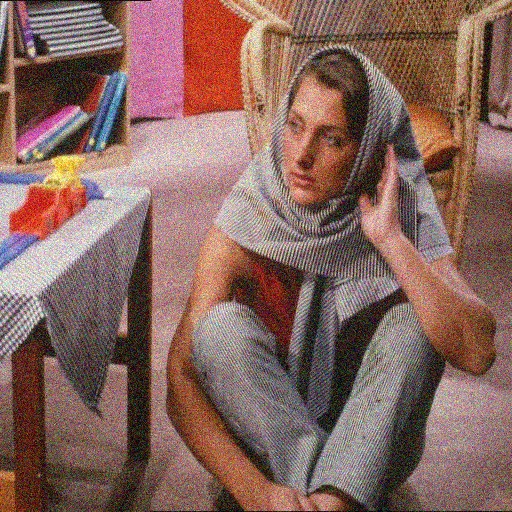
(b) Noisy image

(c) Mean field approximation.

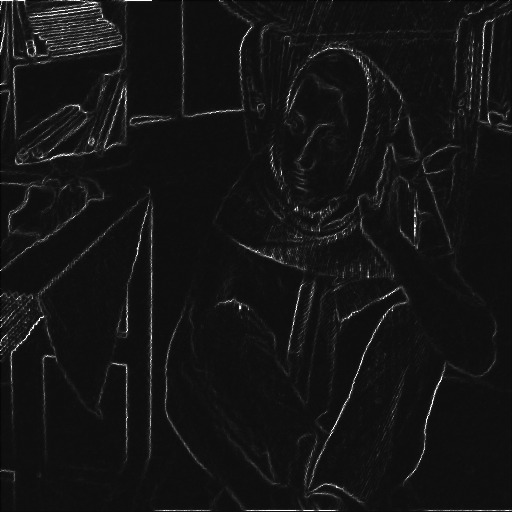
(d) Mean edge image corresponding to mean field approximation

(e) MAP-assignment

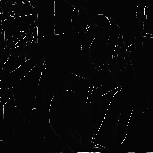
(f) Mean edge weights corresponding to MAP-assignment

Figure 2: Denoising results for Perona-Malik prior with $\lambda=C=10^{3}$ and Gaussian noise with $\sigma=0.1$.

Figure 2e shows the MAP-assignment that we obtained by applying the EM algorithm to the image in Figure 2b and Figure 2c shows the result from the (relaxed) mean field algorithm. We see that the mean field algorithm finds more edges and better restores the finer details in the image. This can also be seen in Figure 2f and Figure 2d, where the corresponding mean edge weights $1/\xi_{0}$ are shown. Whereas the EM algorithm tends to make a binary decision whether a given pixel is part of an edge or not, the mean field algorithm also finds some soft edges and textured areas in the image. Similarly, Figure 3 shows the results obtained by applying the same Perona-Malik-prior as for the denoising problem to a deconvolution problem. Again, we see that the mean field approximation in Figure 3c better captures some of the finer details in the uncorrupted image than the corresponding MAP-assignment in Figure 3d.

(a) Uncorrupted image

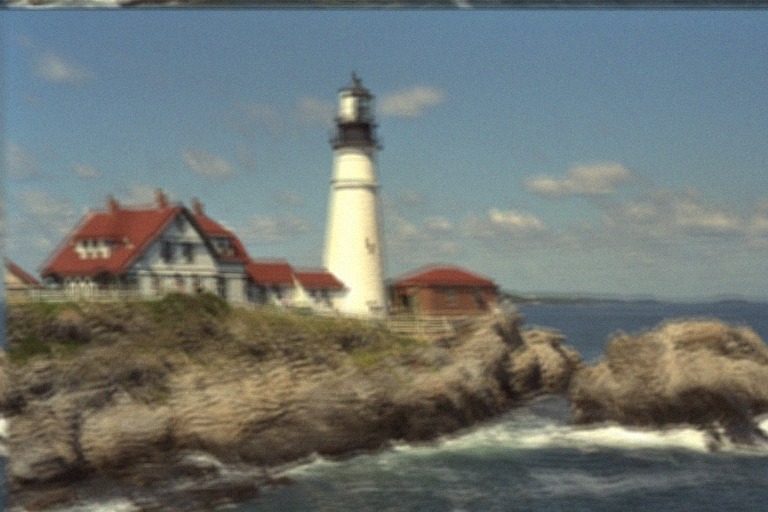
(b) Blurry image

(c) Mean field approximation

(d) MAP-assignment

Figure 3: Deconvolution results for Perona-Malik prior with $\lambda=C=4\cdot 10^{3}$ and Gaussian noise with $\sigma=0.02$.

Our last example shows that also discrete measures $q$ in (5) can be used. A discrete prior for the latent edge weight leads to a binary decision if a pixel is considered to be an edge pixel or not. We define the prior by the counting measure $q$ concentrated on $\{0,\lambda\}$, i.e. $q=\delta_{0}+\delta_{\lambda}$ and use the function $v(z)=-\tfrac{\mu}{\lambda}z$. This yields

$$\psi(t) =-\log\Big{(}\int e^{-\big{(}t-\tfrac{\mu}{\lambda})z}q(dz)\Big{)}$$

$$=-\log\Big{(}\int e^{-\big{(}t-\tfrac{\mu}{\lambda})z}(\delta_{0}+\delta_{\lambda})(dz)\Big{)}$$

$$=-\log\big{(}1+e^{-\lambda t+\mu}\big{)}$$

$$=\log\sigma(\lambda t-\mu),$$

where $\sigma$ is the sigmoid function given by $\sigma(t)=\tfrac{1}{1+\mathrm{e}^{-t}}$. Because $\sigma^{\prime}(t)=\sigma(t)(1-\sigma(t))$, this shows that

$$f(t)=\psi^{\prime}(t)=\lambda\left(1-\sigma(\lambda t-\mu)\right).$$

Intuitively, $z(x)=0$ indicates that a given pixel $x$ belongs to an edge, while $z(x)=\lambda$ indicates the opposite. Note that this prior can therefore be interpreted as a probabilistic version of the Mumford-Shah functional mumford1989optimal . While connections between the Perona-Malik model and the Mumford-Shah model have been observed previously in morini2003mumford where the Mumford-Shah functional appeared as the $\Gamma$-limit of Perona-Malik models for dicretized $\Omega$ while the discretization gets finer and finer, we obtain both models in the same discretized context. Figure 4c shows the conditional mean computed from the Markov chain after $100$ iterations of Gibbs sampling. Figure 4e shows the corresponding MAP-assignment computed using the EM-algorithm. We see that in this case the conditional mean is much better at restoring edges and fine details than the corresponding MAP-assignment. Figure 4d and Figure 4f, which show the corresponding mean edge images, confirm this hypothesis. Better MAP-reconstructions can be obtained by changing the $\mu$-parameter, but this corresponds to a different prior distribution.

(a) Uncorrupted image

(b) Noisy image

(c) Conditional mean

(d) Conditional mean of corresponding edge image

(e) MAP-assignment

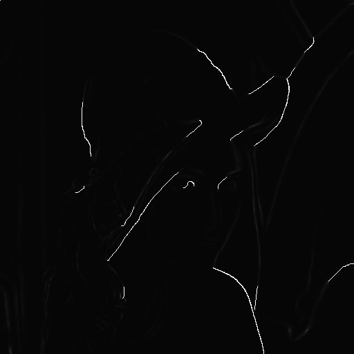
(f) Mean edge weights corresponding to MAP-assignment

Figure 4: Denoising results for the discrete Mumford-Shah-like edge prior with $\lambda=800.0$ and $\mu=3.8$ and Gaussian noise with $\sigma=0.1$.

5 Conclusion

In this work we established the relationship between the celebrated Perona-Malik model with a probabilistic model for image processing. We used Gaussian scale mixtures where we modeled the (inverse) variance of a Gaussian smoothness prior as a latent variable. We proposed different algorithmic approaches to infer information (usually images and edge maps) from the corresponding posterior and all algorithms resemble the lagged-diffusivity scheme for the Perona-Malik model in one way or another. We suspect that the interpretation of the Perona-Malik model as a probabilistic model with a latent variable for the edge prior can be related to the underlying neurological motivation for non-linear diffusion models in human image perception as, e.g. outlined in early works of Grossberg at al., see e.g. cohen1984neural ; grossberg1984outline ; grossberg1985neural .

Our interpretation of the Perona-Malik model as an EM algorithm explains the observed over-smoothing and staircasing in the sense that lagged-diffusivity approximates a MAP estimator of the posterior, which is in general not a good representative of the distribution. Our method based on mean field approximation from Section 3.2 partly avoids this over-smoothing and staircasing effect by explicitly incorporating the uncertainty in the image variable $u$. However, the mean field approach in its plain form leads to a method with high computational cost and we proposed an approximate mean field method in Algorithm 3. The approximation is based on a diagonal approximation $C$ of a covariance matrix. While this already leads to good results, a possible improvement may be to restrict $C$ to the set of $k\times k$ block matrices. Alternatively we could also restrict it to the set of circular matrices. Both approximations can also be combined by setting $C$ to a product of the form

$$C=C_{block}C_{circ}C_{block}^{\intercal}$$

or even

$$C=\left(\prod_{i}C_{block}^{(i)}C_{circ}^{(i)}\right)\left(\prod_{i}C_{block}^{(i)}C_{circ}^{(i)}\right)^{\intercal}$$

yielding better and better approximations to the true covariance matrix.

References

- [1] David F Andrews and Colin L Mallows. Scale mixtures of normal distributions. Journal of the Royal Statistical Society. Series B (Methodological), pages 99–102, 1974.
- [2] Yufang Bao and Hamid Krim. Smart nonlinear diffusion: A probabilistic approach. IEEE Transactions on Pattern Analysis and Machine Intelligence, 26(1):63–72, 2004.
- [3] M. Bertero and P. Boccacci. Introduction to Inverse Problems in Imaging. Institute of Physics Publishing, 1998.
- [4] Jeff Bezanson, Alan Edelman, Stefan Karpinski, and Viral B Shah. Julia: A fresh approach to numerical computing. arXiv preprint arXiv:1411.1607, 2014.
- [5] Tony F Chan and Pep Mulet. On the convergence of the lagged diffusivity fixed point method in total variation image restoration. SIAM Journal on Numerical Analysis, 36(2):354–367, 1999.
- [6] Yunjin Chen, Wei Yu, and Thomas Pock. On learning optimized reaction diffusion processes for effective image restoration. In Proceedings of the IEEE Conference on Computer Vision and Pattern Recognition, pages 5261–5269, 2015.
- [7] Michael A. Cohen and Stephen Grossberg. Neural dynamics of brightness perception: Features, boundaries, diffusion, and resonance. Perception & Psychophysics, 36(5):428–456, 1984.
- [8] Arthur P. Dempster, Nan M. Laird, and Donald B. Rubin. Maximum likelihood from incomplete data via the EM algorithm. Journal of the royal statistical society. Series B (methodological), pages 1–38, 1977.
- [9] Stuart Geman and D. Geman. Stochastic Relaxation, Gibbs Distributions, and the Bayesian Restoration of Images. IEEE Transactions on Pattern Analysis and Machine Intelligence, PAMI-6(6):721–741, November 1984. 17002.
- [10] Stephen Grossberg. Outline of a theory of brightness, color, and form perception. Advances in Psychology, 20:59–86, 1984.
- [11] Stephen Grossberg and Ennio Mingolla. Neural dynamics of perceptual grouping: textures, boundaries, and emergent segmentations. Perception & Psychophysics, 38(2):141–171, 1985.
- [12] Jari Kaipio and Erkki Somersalo. Statistical and computational inverse problems. Number v. 160 in Applied mathematical sciences. Springer, New York, 2005.
- [13] Hamid Krim and Yufang Bao. Nonlinear diffusion: A probabilistic view. In Image Processing, 1999. ICIP 99. Proceedings. 1999 International Conference on, volume 2, pages 21–25. IEEE, 1999.
- [14] Massimiliani Morini and Matteo Negri. Mumford-Shah functional as -limit of discrete Perona-Malik energies. Mathematical Models and Methods in Applied Sciences, 13(06):785–805, 2003.
- [15] David Mumford and Jayant Shah. Optimal approximations by piecewise smooth functions and associated variational problems. Communications on pure and applied mathematics, 42(5):577–685, 1989.
- [16] Kevin P. Murphy. Machine learning: a probabilistic perspective. Adaptive computation and machine learning series. MIT Press, Cambridge, MA, 2012.
- [17] K Niklas Nordström. Biased anisotropic diffusion: a unified regularization and diffusion approach to edge detection. Image and vision computing, 8(4):318–327, 1990.
- [18] George Papandreou and Alan L Yuille. Gaussian sampling by local perturbations. In J. D. Lafferty, C. K. I. Williams, J. Shawe-Taylor, R. S. Zemel, and A. Culotta, editors, Advances in Neural Information Processing Systems 23, pages 1858–1866. Curran Associates, Inc., 2010.
- [19] Pietro Perona and Jitendra Malik. Scale-space and edge detection using anisotropic diffusion. Pattern Analysis and Machine Intelligence, IEEE Transactions on, 12(7):629–639, 1990.
- [20] Aleksandra Pizurica, Iris Vanhamel, Hichem Sahli, Wilfried Philips, and Antonis Katartzis. A Bayesian formulation of edge-stopping functions in nonlinear diffusion. IEEE Signal Processing Letters, 13(8):501–504, 2006.
- [21] Otmar Scherzer, Markus Grasmair, Harald Grossauer, Markus Haltmeier, and Frank Lenzen. Variational methods in imaging, volume 167 of Applied Mathematical Sciences. Springer, New York, 2009.
- [22] Uwe Schmidt, Qi Gao, and Stefan Roth. A generative perspective on MRFs in low-level vision. In Computer Vision and Pattern Recognition (CVPR), 2010 IEEE Conference on, pages 1751–1758. IEEE, 2010.
- [23] Curtis R Vogel and Mary E Oman. Iterative methods for total variation denoising. SIAM Journal on Scientific Computing, 17(1):227–238, 1996.
- [24] Martin J. Wainwright and Michael I. Jordan. Graphical Models, Exponential Families, and Variational Inference. Found. Trends Mach. Learn., 1(1-2):1–305, January 2008.
- [25] Joachim Weickert. Anisotropic diffusion in image processing. Teubner Stuttgart, 1998.
- [26] Guoshen Yu, Guillermo Sapiro, and Stéphane Mallat. Image modeling and enhancement via structured sparse model selection. In 2010 IEEE International Conference on Image Processing, pages 1641–1644. IEEE, 2010.