A modified Physarum-inspired model for the user equilibrium traffic assignment problem

Abstract

The user equilibrium traffic assignment principle is very important in the traffic assignment problem. Mathematical programming models are designed to solve the user equilibrium problem in traditional algorithms. Recently, the Physarum shows the ability to address the user equilibrium and system optimization traffic assignment problems. However, the Physarum model are not efficient in real traffic networks with two-way traffic characteristics and multiple origin-destination pairs. In this article, a modified Physarum-inspired model for the user equilibrium problem is proposed. By decomposing traffic flux based on origin nodes, the traffic flux from different origin-destination pairs can be distinguished in the proposed model. The Physarum can obtain the equilibrium traffic flux when no shorter path can be discovered between each origin-destination pair. Finally, numerical examples use the Sioux Falls network to demonstrate the rationality and convergence properties of the proposed model.

1 INTRODUCTION

The traffic assignment refers to a manner in which a given aggregate origin-destination (OD) pair passenger traffic demand is assigned to the traffic routes of that OD pair[1, 2, 3, 4, 5]. As an important traffic assignment paradigm, the user equilibrium (UE) of travelers’ path choice in traffic networks was firstly conceptualised by Wardrop [6]. The UE principle is based on the assuming that the traveller knows the precise route cost and will choose the route with the minimum cost. The user equilibrium is achieved when all travellers between the same OD pair have the same and minimum cost [7, 8]. Additionally, the transportation cost of any traveller can’t be reduced by unilaterally changing routes.

In the existing literatures, many algorithms were designed to address the UE problem [9, 10, 11], which can be totally classed into three types: link based algorithms, path based algorithms and origin based algorithms. The linear approximation method of Frank and Wolfe (FW) [12] has been the most popular algorithm in practice because of its simplicity. As a linear approximation method, the FW algorithm has a sublinear asymptotic convergence speed [9]. As a consequence, highly precise solutions can’t be achieved within reasonable computation time. In path based algorithms, the UE problem is solved by achieving the path flux directly [13]. The traffic flux is assigned by fixing the flux from other OD pairs for each OD pair. In the exiting path based algorithms, the disaggregate simplicial decomposition algorithm (DSD) [14] and the gradient projection algorithm (GP) [15, 16, 9] are widely used. Both DSD and GP have shown excellent results when compared with FW algorithm [17, 18], but the memory requirement is usually regarded as impractical for large-scale networks. The origin based algorithm proposed by Bar-Gera [19, 20] doesn’t require as much memory as the path based algorithms. The algorithm computes sequentially for each origin subnetwork by using a quasi-Newton approach. Later, Dial [21] developed a different origin based algorithm by shifting flows sequentially from the longest to the shortest path. Though the origin based algorithms can provide both link traffic flows and route traffic flows [22], enumerating all route flows of each subnetwork is quite complicated.

Biological systems usually inspire computer scientists and engineers to process the information and make decisions. So far, some heuristic algorithms have been proposed to solve the traffic assignment problem, such as the ant colony algorithm [23, 24] and the genetic algorithm [25]. Recently, the slime mould Physarum polycephalum becomes a popular living computing substrate [26, 27]. Physarum machines are proved to be the most successful biological substrates in solving problems of computation geometry, optimization, and logic because they are easy to realize [28]. In this article, a modified Physarum-inspired model is proposed to solve the UE traffic assignment problem.

Physarum polycephalum is a large amoeboid organism, which contains a great number of nuclei and tubular structures [29]. These tubular structures will distribute protoplasm as a transportation network. The experiment has shown that the Physarum has the capacity of finding the short path between two points in a given labyrinth [30]. A mathematical model can capture the basic dynamics of network adaptability through iterations of local rules and produces solutions with properties comparable to or better than those of real-world infrastructure networks [31]. The convergence of Physarum finding the shortest path has been proved by Bonifaci et al. [32]. Based on its foraging behavior, so far, the Physarum has been used to solve many problems, such as finding the shortest path in directed or undirected network [33, 34, 35, 36], designing and simulating transport network [37, 38, 39, 40], natural implementation of spatial logic [41, 42], and computer music [43, 44, 45]. In addition, the Physarum model can also find the shortest path under uncertain environment [46, 47] in the real application [48].

Recently, quite a few researchers try to apply the Physarum model to solve the traffic assignment problem [49, 50]. These Physarum-inspired models can affect well in specific conditions where networks are unilaterally connecting. But the exiting models can’t be realised in traffic networks with two-way traffic characteristics. The Physarum model for UE traffic assignment problem [50] can’t distinguish the flux from different OD pairs, which means the model isn’t reasonable in traffic networks with multiple OD pairs. In this paper, a modified Physarum-inspired model for the UE traffic assignment problem is proposed for traffic networks with two-way traffic characteristics. In the proposed model, the flows are decomposed by origin node as the origin based algorithms. For each subnetwork, the flows are assigned by the Physarum model based on its protoplasmic network adaptivity and continuity.

This paper is structured as follows. In Section 2, the user equilibrium traffic assignment principle is reviewed. The original Physarum polycephalum model and Physarum-inspired model for UE traffic assignment problem proposed by Zhang [50] are briefly introduced. In Section 3, a modified Physarum-inspired model for the UE traffic assignment problem is presented. In Section 4, numerical examples are given to demonstrate the rationality and convergence properties of the proposed model. Finally, the paper ends with conclusions and suggestions for further researches in Section 5.

2 PRELIMINARIES

In this section, some preliminaries are briefly introduced, including the traffic assignment model [7], the original Physarum polycephalum model [51] and the Physarum-inspired model for UE problem proposed by Zhang [50].

2.1 User Equilibrium Traffic Assignment Model

The transportation network is a strongly connected directed graph ${G(N,A)}$, where $N$ is the set of nodes and $A$ is the set of directed links. Assume that there is no links from a node to itself and only one link, if any, between two different nodes. Suppose that $R$ and $S$ denote the set of origin nodes and the set of destination nodes, and $r\in R$, $s\in S$, $R,S\subseteqq N$. Let $K_{rs}$ and $q_{rs}$ denote the set of all the paths and the travel demand between OD pair $r-s$, than we have:

$$\sum\limits_{k\in{K_{rs}}}{f_{k}^{rs}}={q_{rs}},~{}~{}~{}{\rm{}}\forall r\in R,s\in S$$ (1)

where $f_{k}^{rs}$ is the path traffic flow along path $k$ between OD pair $r-s$. Let $x_{a}$ denote the traffic flow along the link $a$. Then all nodes, except source nodes and destination nodes, satisfy the flow conservation law [50], shown as follows:

$$\sum\limits_{a\equiv[(i,j)\in A]}{{x_{a}}}=\sum\limits_{b\equiv[(j,k)\in A]}{{x_{b}}},\forall j,k\in N\backslash\{R,S\}$$ (2)

Let $t_{a}(x_{a})$ denote the traffic time experienced by each user among the link $a$ when $x_{a}$ units of vehicles flux along the link. $t_{a}(.)$ is a monotonously non decreasing and continuously differentiable traffic time functions for the flux on link $a$ due to the effects of congestion on the travel time [7], which can be expressed as follows:

$$~{}~{}~{}~{}~{}\frac{{\partial{t_{a}}({x_{a}})}}{{\partial{t_{b}}}}=0,~{}~{}~{}\forall a\neq b$$ (3)

$$\frac{{\partial{t_{a}}({x_{a}})}}{{\partial{x_{a}}}}>0,~{}~{}~{}\forall a$$ (4)

Let $c_{k}^{rs}$ represent the path traffic time along the path $k$ between OD pair $r-s$ and $\delta_{a,k}^{rs}$ denote the correlation coefficient between traffic link and traffic path, $\delta_{a,k}^{rs}=1$ if the $k_{th}$ path between OD pair $r-s$ traverses link $a$, otherwise $\delta_{a,k}^{rs}=0$. The path traffic time $c_{k}^{rs}$ and link traffic flow $x_{a}$ can be expressed as [7]:

$$c_{k}^{rs}=\sum\limits_{a}{{t_{a}}}\cdot\delta_{a,k}^{rs}~{}~{}~{}{\rm{}}\forall r,s,k$$ (5)

$${x_{a}}=\sum\limits_{r}{\sum\limits_{s}{\sum\limits_{k}{f_{k}^{rs}\cdot\delta_{a,k}^{rs}}}},~{}~{}~{}\forall a$$ (6)

The Wardrop’s user equilibrium principle [6] is that travelers seek to minimize the cost associated with their chosen routes. Travelers are assumed to have perfect information about actual travel conditions, and they can be identical in the sense that they valued time, monetary cost, and other route attributes in the same way. The Wardrop’s user equilibrium is obtained when no traveller s traffic time can be reduced by unilaterally changing routes, which can be expressed as follows:

$${u_{rs}}-c_{k}^{rs}\left\{\begin{array}[]{l}=0,~{}~{}~{}f_{k}^{rs}>0\\ \leq 0,~{}~{}~{}f_{k}^{rs}{\rm{=}}0\\ \end{array}\right.,~{}~{}~{}\forall k,r,s$$ (7)

where $u_{rs}$ is the shortest traffic time between OD pair $r-s$ under traffic equilibrium.

Under the assumptions above all, the traffic assignment problem can be mathematically formulated as the following convex optimization problem [7]:

$$\begin{array}[]{l}\min Z(x)=\sum\limits_{a}{\int_{0}^{{x_{a}}}{{t_{a}}(w)dw}}\\ s.t.\\ ~{}~{}~{}~{}~{}~{}{x_{a}}=\sum\limits_{r}{\sum\limits_{s}{\sum\limits_{k}{f_{k}^{rs}\cdot\delta_{a,k}^{rs}}}},~{}~{}~{}\forall a\\ ~{}~{}~{}\sum\limits_{[(i,j)\in A]}{{x_{a}}}=\sum\limits_{[(j,k)\in A]}{{x_{b}}},~{}~{}~{}~{}~{}~{}~{}\forall j,k\in N\backslash\{R,S\}\\ ~{}~{}~{}~{}~{}~{}\sum\limits_{k}{f_{k}^{rs}}={q_{rs}},~{}~{}~{}~{}~{}~{}~{}~{}~{}~{}~{}~{}~{}~{}~{}~{}\forall r,s\\ ~{}~{}~{}~{}~{}~{}f_{k}^{rs}\geq 0,~{}~{}~{}~{}~{}~{}~{}~{}~{}~{}~{}~{}~{}~{}~{}~{}~{}~{}~{}~{}~{}~{}\forall k,r,s\\ ~{}~{}~{}~{}~{}~{}x_{a}\geq 0,~{}~{}~{}~{}~{}~{}~{}~{}~{}~{}~{}~{}~{}~{}~{}~{}~{}~{}~{}~{}~{}~{}~{}\forall a\end{array}$$ (8)

2.2 The Origin Physarum Polycephalum Model

Physarum polycephalum is a single-celled amoeboid organism, which is also called as plasmodium in the vegetative phase [51]. It has the ability to solve the shortest path selection, based on its special foraging mechanism: the transformations of tubular structures and a positive feedback from flow rates. The high rates of the flow motivate tubes to thicken and the diameter of the tube minishes at a low flow rate [51]. A total introduction for the physarum polycephalum path finding model is given below.

Suppose the shape of the network formed by the Physarum is represented by a graph $G(N,A)$, where the edge of the graph denotes the plasmodial tube and the node denotes the junction between tubes. And $N$ is a set of nodes, where $N_{1}$ and $N_{2}$ are signed as the source and destination nodes, any others are labeled as $N_{3}$, $N_{4}$, $N_{5}$, etc. The edge connecting node $i$ and node $j$ are remarked as $M_{ij}$ and the flux from node $N_{i}$ to node $N_{j}$ through edge $M_{ij}$ is remarked as ${Q_{ij}}$, shown as follows [51]:

$${Q_{ij}}=\frac{{\pi{\rm{r}}_{ij}^{4}}}{{8\eta{L_{ij}}}}({p_{i}}-{p_{j}})=\frac{{{D_{ij}}}}{{{L_{ij}}}}({p_{i}}-{p_{j}})$$ (9)

where $\eta$ is the viscosity of the fluid and ${D_{ij}}{\rm{=}}\pi{\rm{r}}_{ij}^{4}/8\eta$ is the measure of the conductivity of the edge tube $M_{ij}$. And $p_{i}$ is the measure of the pressure at the node $n_{i}$, $L_{ij}$ is the length of the edge $M_{ij}$. According to the conservation law of flow, the inflow and outflow must be balanced, namely:

$$\sum{{Q_{ij}}=}0,~{}~{}~{}{\rm{}}({\rm{j}}\neq{\rm{1,2}})$$ (10)

especially for the source nodes $N_{1}$ and $N_{2}$, the flux equations can be expressed as:

$$\sum\limits_{i}{{Q_{i1}}}+{I_{0}}=0$$ (11)

$$\sum\limits_{i}{{Q_{i2}}}-{I_{0}}=0$$ (12)

where $I_{0}$ is the flux from the source node to the destination node, which is assumed as a constant in the model. According to the Eqs.(9-12), the network Poisson equation for the pressure is derived as following:

$$\sum\limits_{i}{\frac{{{D_{ij}}}}{{{L_{ij}}}}({p_{i}}-{p_{j}})}=\left\{\begin{array}[]{l}-1~{}~{}~{}~{}~{}{\rm{}}for~{}{\rm{}}j=1,\\ +1~{}~{}~{}~{}~{}{\rm{}}for~{}{\rm{}}j=2,\\ 0~{}~{}~{}~{}~{}~{}~{}{\rm{}}otherwise{\rm{}}{}{}{}\\ \end{array}\right.$$ (13)

by further setting $p_{2}=0$ as the basic pressure level, the pressure of all nodes can be determined, the pressure of all nodes can be determined according to Eq.(13) and all $Q_{ij}$ can be determined by solving Eq.(9).

To accommodate the adaptive behavior of the plasmodium, the conductivity $D_{ij}$ is assumed to change when adapting to the flux $Q_{ij}$. And tubes with zero conductivity will die out. The conductivity of each tube is described as follows: [31]:

$$\frac{d}{{dt}}{D_{ij}}=f(|{Q_{ij}}|)-\alpha{D_{ij}}$$ (14)

where $\alpha$ is the decay rate of the tube and $f(.)$ is monotonously increasing continuous function which satisfies $f(0)=0$. Obviously, the positive feedback exists in the model.

2.3 The Physarum-inspired Model for UE Problem

According to the feature of Physarum foraging behavior system, the optimum problem and the user equilibrium problem in directed traffic networks are solved by modified Physarum models [49, 50] . There are mainly two points different from from the original Physarum model in Zhang’s method [50].

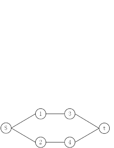
(a) The origin model

(b) The model modified by Zhang [50]

Figure 1: Simple networks for Physarum model

First, the original Physarum model can only find the shortest path in undirected networks shown in Figure 1(a). The modified method was proposed to extend the original Physarum model to directed networks. A total introduction for the modified model is given below.

In the modified model, each edge is regard as two tubes with opposite directions and equal weight, which is shown in Figure 1(b). And there is only one direction between two nodes in the network, which means that flux can only flow from node $s$ to node $1$ and it can’t flow in the opposite direction as shown in Figure 1(b). And the network Posson equation defined in Eq.(13) was modified as follows [50]:

$$\sum\limits_{i}{(\frac{{{D_{ij}}}}{{{L_{ij}}}}+\frac{{{D_{ji}}}}{{{L_{ji}}}})+({p_{i}}-{p_{j}})}=\left\{\begin{array}[]{l}-1~{}~{}~{}~{}~{}{\rm{}}for~{}{\rm{}}j=1,\\ +1~{}~{}~{}~{}~{}{\rm{}}for~{}{\rm{}}j=2,\\ 0~{}~{}~{}~{}~{}~{}~{}{\rm{}}otherwise{\rm{}}{}{}{}\\ \end{array}\right.$$ (15)

where $L_{ij}$ denotes the travel time of from node $i$ to node $j$ and $L_{ji}$ denotes the travel time of from node $j$ to node $i$. Similarly, $D_{ij}$ and $D_{ji}$ have different meanings. In the initialization, if $L_{ij}=inf$, then $D_{ij}=0$. Otherwise, assign a value between $0$ and $1$ to $D_{ij}$. To guarantee the inconsistency, $Q_{ij}$ should be kept $0$ during iterations if $L_{ij}=inf$.

Second, there is only one source and one destination in networks. However, usually there are multiple OD pairs in traffic networks. To handel the network with multiple origins and destinations, Eq.(15) was modified as follows [50]:

$$\sum\limits_{i}{(\frac{{{D_{ij}}}}{{{L_{ij}}}}+\frac{{{D_{ji}}}}{{{L_{ji}}}})({p_{i}}-{p_{j}})}=\left\{\begin{array}[]{l}-{I_{r}},~{}~{}~{}~{}~{}{\rm{}}\forall r\in R,\\ +{I_{s}},~{}~{}~{}~{}~{}{\rm{}}\forall s\in s,\\ 0,~{}~{}~{}~{}~{}~{}~{}~{}~{}{\rm{}}otherwise\\ \end{array}\right.$$ (16)

where $r$ denotes the origin node and $r\in R$, $s$ denotes the destination node and $s\in S$. $I_{r}$ and $I_{s}$ represent the units of flow supplied by the origin node $r$ and consumed by the destination node $s$.

3 PROPOSED METHOD

In this section, we will discuss the shortcomings of the original Physarum-inspired method for UE problem and propose the modified Physarum-inspired method to solve the UE problem.

3.1 Shortcomings of the Origin Physarum-inspired Method

Compared with the previous slime mould models, the Physarum-inspired method for UE problem is superior when characterizing its foraging activity. However, two shortcomings of the original Physarum-inspired method for UE problem are founded as follows:

1. Note that there is only one direction between two nodes in the network shown in Figure 1(b), which means the flux can only flow from one node to another but never in the opposite direction. However, in real traffic networks, most roads have the properties of two-way traffic characteristics as shown in Figure 2. Clearly, opposite directions are separated with each other, where flows don’t interfere in two opposite directions. Obviously, the original Physarum-inspired method can’t be implemented in the traffic network shown in Figure 2.

   

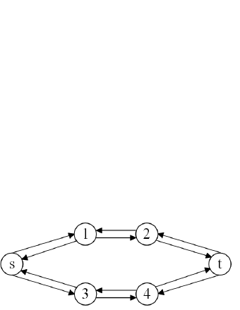
   Figure 2: The real traffic network

2. The Physarum-inspired model for UE problem isn’t reasonable in traffic networks with multiple OD pairs. The modified equation Eq.(16) only satisfies the flow conservation law of the traffic network. However, it can’t distinguish the flux in each OD pair, which means that for a given OD pair $r-s$, the output flux at node $s$ doesn’t equal the input flow at node $r$. In fact, the Physarum-inspired model for UE problem is only suitable for traffic networks with one source and multiple sinks or multiple sources and one sink. Here, we illustrate this problem with the following example.

Example   A small network with multiple sources and multiple sinks

Here, we use a small traffic network with 4 nodes, 4 links and 2 OD pairs which are shown in Figure 3. And the origin-destination demands, in vehicles per hour, are $q_{1,2}$=100 and $q_{4,3}=100$. For simplicity, the link travel time is calculated by the US Bureau of Public Roads(BPR) function [52], which is expressed as follows:

$${t_{a}}={\alpha_{a}}(1+0.15{(\frac{{{Q_{a}}}}{{{c_{a}}}})^{4}})$$ (17)

where $t_{a}$, $\alpha_{a}$, $Q_{a}$, $c_{a}$ denote the travel time, free flow travel time flow and the capacity on link $a$, respectively.

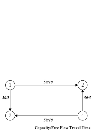
Figure 3: A small traffic network

By using the Physarum-inspired model, the path flows are shown in Table 1. It’s clear that traffic assignment doesn’t satisfy the traffic demands, which the flux along path $1\rightarrow 3$ and path $4\rightarrow 2$ should equal 100. Note that the free flow travel time of $1\rightarrow 3$ and $4\rightarrow 2$ is much less than that of $1\rightarrow 2$ and $4\rightarrow 3$. Clearly the model doesn’t distinguish the flux from different OD pairs. As a result, the Physarum-inspired model assigns more flux to path $1\rightarrow 3$ and $4\rightarrow 2$.

Table 1: Path flows of the traffic network shown in Figure 3

Path(node sequence)	Path flow	Path cost
1 $\rightarrow$ 2	19.5177	10.0348
1 $\rightarrow$ 3	80.4823	10.0348
4 $\rightarrow$ 2	80.4823	10.0348
4 $\rightarrow$ 3	19.5177	10.0348

3.2 The Modified Physarum-inspired Model for UE Problem

Here, we proposed a modified physarum-inspired model for UE problem to overcome these above-mentioned shortcomings.

3.2.1 Modified Physarum model for the shortest path in directed networks

To satisfy the characteristic of the real traffic network shown in Figure 2, each edge is regarded as two tubes with opposite directions and different weight. And flux can flow in opposite directions without interfering with each other. The network Posson equation is same as Eq.(15). But to maintain the validity of conductivity, the conductivity equation defined in Eq.(9) should be improved as follows:

$${Q_{ij}}=\left\{\begin{array}[]{l}\frac{{{D_{ij}}}}{{{L_{ij}}}}({p_{i}}-{p_{j}}),~{}~{}~{}~{}~{}{\rm{}}\frac{{{D_{ij}}}}{{{L_{ij}}}}({p_{i}}-{p_{j}})>0\\ 0,~{}~{}~{}~{}~{}~{}~{}~{}~{}~{}~{}~{}~{}~{}~{}~{}~{}~{}~{}{\rm{}}otherwise{\rm{}}{}{}{}\\ \end{array}\right.$$ (18)

when the flux in each tube is negative, the flux will be assigned as 0. That’s because the flux can’t get through the given tube in the opposite direction. In the initialization, if ${L_{ij}\neq inf}$, we assign a value between 0 and 1 to ${D_{ij}}$. Otherwise, conductivity ${D_{ij}}$ is assigned as $0$.

Particularly, when $L_{ij}=inf$ or $L_{ji}=inf$, which means that the flux can only flow from node $j$ to node $i$ or from node $i$ to node $j$, our modified model is the same as that introduced in Sec. 2.3. Exactly, the model shown in Sec. 2.3 is a special case of our modified model.

3.2.2 Modified Physarum model for directed networks with sources and multiple sinks

To overcome the defect that the Physarum-inspired model can’t distinguish the flux in each OD pair, we modify the Physarum-inspired model as below. Let $S_{r}$ denote the set of destination nodes which are originated from node $r$. Clearly, we have:

$${I_{r}}=\sum\limits_{s\in S_{r}}{{I_{rs}}}$$ (19)

where $I_{r}$ denotes the input flow at the origin node $r$ and $I_{rs}$ denotes the output flow at the destination node $s$ originated from node $r$. Here, we regard the multiple sources and multiple sinks network as the superposition of one source and multiple sinks networks. For each one source and multiple sinks network, we modify the original network Poisson equation Eq.(13) as follows:

$$\sum\limits_{i}{(\frac{{{D_{ij}}}}{{{L_{ij}}}}+\frac{{{D_{ji}}}}{{{L_{ji}}}})({p_{i}}-{p_{j}})}=\left\{\begin{array}[]{l}-{I_{r}},~{}~{}~{}~{}~{}{\rm{}}for~{}~{}j=r,\\ +{I_{rs}},~{}~{}~{}~{}~{}{\rm{}}\forall s\in S_{rs},\\ 0,~{}~{}~{}~{}~{}~{}~{}~{}~{}{\rm{}}otherwise\\ \end{array}\right.$$ (20)

Naturally, the flux of each tube in all one source and multiple sinks subnetworks can be calculated by Eq.(18). According to the superposition principle, the flux of each tube in the original multiple sources and sinks network can be expressed as follows:

$$Q_{ij}^{all}=\sum\limits_{r\in R}{Q_{ij}^{r}},~{}~{}~{}\forall i,j\in N$$ (21)

where $Q_{ij}^{all}$ denotes the flux from node $i$ to node $j$ in the original multiple sources and multiple sinks network and $Q_{ij}^{r}$ represents the flux from node $i$ to node $j$ in the subnetwork originated from node $r$.

3.2.3 Modified Physarum model for UE problem

Note that in the process of Phyasrun approaching the shortest path, the flow and the conductivity along each link are continuous. Further consideration of the continuity and dynamic reconfiguration of Physarum model, we can update the link travel time within each iteration. The flux will be redistributed by the modified Physarum model when the link travel time is updated during iterations. The length of link $a$ is updated as follows:

$$L_{a}^{n+1}=\frac{{L_{a}^{n}+{t_{a}}(Q_{a}^{all_{n+1}})}}{2}$$ (22)

where $Q_{a}^{all_{n+1}}$ denotes the total flow on link $a$ at the $(n+1)_{th}$ iteration, $L_{a}^{n}$ and $L_{a}^{n+1}$ represent the length of link $a$ at the $n_{th}$ and $(n+1)_{th}$ iteration. And the search direction of link length $L_{a}$ is guided by ${t_{a}}(Q_{a}^{all_{n+1}})$. Note that in equilibrium, there will be $L_{a}=t_{a}(Q_{a}^{all})$, which means the length of link $a$ equals the travel time along link $a$.

Here, the main steps of the modified Physarum-inspired model for user equilibrium problem is presented in Algorithm 1.

Algorithm 1 Modified Physarum-inspired model for UE problem

// $Q^{r}$ is the flow matrix of the subnetwork originated from node $r$.

// $L^{0}$ is the free flow travel time matrix.

$D_{ij}^{r}=[0.5,1](\forall i,j=1,2,\cdots,N\wedge C_{ij}^{0}\neq 0,\forall r\in R)$

if $C_{ij}^{0}==inf$ then

     $D_{ij}^{r}=0$

end if

$Q_{ij}^{r}=0(\forall i,j=1,2,\cdots,N,\forall r\in R)$

${Q_{ij}^{all_{1}}}=0(\forall i,j=1,2,\cdots,N)$

$L_{ij}^{1}=L_{ij}^{0}(\forall i,j=1,2,\cdots,N)$

$n=1$ //Iteration counter

while $NotConvergence$ do

     for $r\in R$ do

         //Calculate the pressure of every node using Eq.(20)

         $\sum\limits_{i}{(\frac{{{D_{ij}^{r}}}}{{{L_{ij}}}}+\frac{{{D_{ji}^{r}}}}{{{L_{ji}}}})({p_{i}}-{p_{j}})}=\left\{\begin{array}[]{l}-{I_{r}},~{}~{}~{}~{}~{}{\rm{}}for~{}~{}j=r,\\ +{I_{rs}},~{}~{}~{}~{}~{}{\rm{}}\forall s\in S_{rs},\\ 0,~{}~{}~{}~{}~{}~{}~{}~{}~{}{\rm{}}otherwise\\ \end{array}\right.$

         //Calculate the flux of every edge using Eq.(18)

         ${Q_{ij}^{r}}=\left\{\begin{array}[]{l}\frac{{{D_{ij}^{r}}}}{{{L_{ij}}}}({p_{i}}-{p_{j}}),~{}~{}~{}~{}~{}{\rm{}}\frac{{{D_{ij}^{r}}}}{{{L_{ij}}}}({p_{i}}-{p_{j}})>0\\ 0,~{}~{}~{}~{}~{}~{}~{}~{}~{}~{}~{}~{}~{}~{}~{}~{}~{}~{}~{}{\rm{}}otherwise{\rm{}}{}{}{}\\ \end{array}\right.$

         ${\rm{D}}_{ij}^{r}=({\rm{D}}_{ij}^{r}+{Q_{ij}^{r}})/2,~{}~{}~{}\forall i,j\in N$

     end for

     $Q_{ij}^{all_{n+1}}=\sum\limits_{r\in R}{Q_{ij}^{r}},~{}~{}~{}\forall i,j\in N$

     $L_{ij}^{n+1}=\frac{{L_{ij}^{n}+{t_{a}}(Q_{ij}^{all_{n+1}})}}{2}$

     $n=n+1$

end while

3.3 Discussion

Usually, there are three convergence measures for the traffic assignment [20, 53], which are briefly introduced as follows:

1. According to the error of traffic flows or travel time calculated in two adjacent times to decide whether the iteration stops [12]. The computing will stop only when the flows become stable in two adjacent iterations. The measure is simple and usually effective, which can get the flows satisfying the UE principle. Naturally the convergence principle can be expressed as follows:

   $$\left|{Q_{ij}^{all_{n+1}}-Q_{ij}^{all_{n}}}\right|\leqslant\varepsilon~{}or~{}\left|{L_{ij}^{n+1}-L_{ij}^{n}}\right|\leqslant C~{}~{}~{}\forall i,j\in N$$ (23)

2. According to the error between the travel time path-based and link-based network, the relative gap (RGAP) and normalized gap (or excess average cost) are taken into consideration to measure the convergence [9]. The measure of RGAP can be expressed as:

   $$\small RGAP=\frac{{({\rm{total~{}travel~{}time}}-{\rm{total~{}travel~{}time~{}on~{}shortest~{}paths}})}}{{{\rm{total~{}travel~{}time}}}}$$ (24)

3. The error between the maximum path travel time and the minimum path travel time between the OD pair is also an evaluation index of convergence [20]:

   $${\varepsilon_{rs}}=\max\{c_{k}^{rs}|k\in{K^{rs}},f_{k}^{rs}>0\}-\min\{c_{k}^{rs}|k\in{K^{rs}}\}$$ (25)

   by giving a suitable value to $\varepsilon_{rs}$, the UE principle can be archived.

Usually, Principle 1 is used in the link based method, such as the FW method. Principle 2 is usually used in the path-based method and Principle 3 is generally used in the origin-based algorithm. Note that the modified Physarum-inspired model for UE problem is actually basing on the link travel time. During iterations, the shortest travel paths and the maximum path travel time aren’t available. In order to reduce computing time, we choose the Principle 1 as the convergence measure in this article, which can be expressed as:

$$\sum\limits_{i,j\in N}{\left|Q_{ij}^{all_{n+1}}{\rm{-}}Q_{ij}^{all_{n}}\right|}\leqslant\varepsilon_{0},~{}~{}~{}\forall i,j\in N$$ (26)

In the proposed Physarum-inspired algorithm, solving a linear system of equations is necessary for each origin based subnetwork. Note that many investigations about paralleled Physarum model have been achieved [54], it’s clear that the paralleled computing can be implemented for each origin based subnetwork. Besides, the linear system of equations for each origin based subnetwork is very special and can be formulated as Laplacian system, which is solvable in $O(m\log n)$ [55]. For the sake of simplicity, paralleled computing isn’t implemented in the following. And the linear system of equations for each origin based subnetwork is solved in a general method with $O(n^{3})$.

4 NUMERICAL EXAMPLES

In this section, numberical examples are illustrated to demonstrate the rationality and convergence properties of the modified method. And the effect of the stopping criterion $\varepsilon_{0}$ is further discussed.

Computational examples reported in this article are using Matlab on Intel(R) Core(TM) i5-5200U processor (2.2Ghz) with 8.00 GB of RAM under Windows Eight.

4.1 Example 1

Here, we use the simple network shown in Figure 3 and the OD demands are same as those showed in Sec. 3.1. By utilizing the modified Physarum-inspired model, the path flows are shown in Table 2. It’s clear that the modified Physarum-inspired model has the ability of distinguishing the flux in different OD pairs.

Table 2: Path flows resulted from the modified method

stopping criterion($\varepsilon_{0}$)	Path(node sequence)	Path flow	Iteration
0.01	1 $\rightarrow$ 2	100	17
	4 $\rightarrow$ 3	100

4.2 Example 2

In this example, we test the modified Physarum-inspired model on the Sioux Falls network [12] which is used in many publications for the traffic assignment problem.

OD flows are given in thousands of vehicles per day, with integer values up to 44 [12]. OD flows here are the values from the table multiplied by 100. They are therefore 0.1 of the original daily flows, and in that sense might be viewed as approximate hourly flows. The parameters in [12] are given as:

$${t_{ij}}=a+b{Q_{ij}}^{4}$$ (27)

where $a$ denotes the free flow travel time given here. The original parameter $b$ can be expressed as:

$${b}=B\cdot\frac{{{\alpha}}}{{{c^{Power}}}}$$ (28)

where $\alpha$ and $c$ denote the free flow traffic time and the capacity flow, respectively. $Power$ is set as $4$ and assume the traditional BPR value of $B=0.15$, so we can get the same travel time equation as Eq.(17). And the free flow travel time($\alpha$) and the capacity flow($c$) are shown in Table 3.

Table 3: Capacity flow($c$) and free flow travel time($\alpha$) along links

ARC	$c(10^{4})$	$\alpha$	ARCS	$c(10^{4})$	$\alpha$	ARCS	$c(10^{4})$	$\alpha$	ARCS	$c(10^{4})$	$\alpha$
$(1,2)$	2.5900	6	$(1,3)$	2.3403	4	$(2,1)$	2.5900	6	$(2,6)$	0.4958	5
$(3,1)$	2.3403	4	$(3,4)$	1.7111	4	$(3,12)$	2.3403	4	$(4,3)$	1.7111	4
$(4,5)$	1.7783	2	$(4,11)$	0.4909	6	$(5,4)$	1.7783	2	$(5,6)$	0.4948	4
$(5,9)$	1.0000	5	$(6,2)$	0.4958	5	$(6,5)$	0.4948	4	$(6,8)$	0.4899	2
$(7,8)$	0.7842	3	$(7,18)$	2.3403	2	$(8,6)$	0.4899	2	$(8,7)$	0.7842	3
$(8,9)$	0.5050	10	$(8,16)$	0.5046	5	$(9,5)$	1.0000	5	$(9,8)$	0.5050	10
$(9,10)$	1.3916	3	$(10,9)$	1.3916	3	$(10,11)$	1.0000	5	$(10,15)$	1.3512	6
$(10,16)$	0.4855	4	$(10,17)$	0.4994	8	$(11,4)$	0.4909	6	$(11,10)$	1.0000	5
$(11,12)$	0.4909	6	$(11,14)$	0.4877	4	$(12,3)$	2.3403	4	$(12,11)$	0.4909	6
$(12,13)$	2.5900	3	$(13,12)$	2.5900	3	$(13,24)$	0.5091	4	$(14,11)$	0.4877	4
$(14,15)$	0.5128	5	$(14,23)$	0.4925	4	$(15,10)$	1.3512	6	$(15,14)$	0.5128	5
$(15,19)$	1.4565	3	$(15,22)$	0.9599	3	$(16,8)$	0.5046	5	$(16,10)$	0.4855	4
$(16,17)$	0.5230	2	$(16,18)$	1.9680	3	$(17,10)$	0.4994	8	$(17,16)$	0.5230	2
$(17,19)$	0.4824	2	$(18,7)$	2.3403	2	$(18,16)$	1.9680	3	$(18,20)$	2.3403	4
$(19,15)$	1.4565	3	$(19,17)$	0.4824	2	$(19,20)$	0.5003	4	$(20,18)$	2.3403	4
$(20,19)$	0.5003	4	$(20,21)$	0.5060	6	$(20,22)$	0.5076	5	$(21,20)$	0.5060	6
$(21,22)$	0.5230	2	$(21,24)$	0.4885	3	$(22,15)$	0.9599	3	$(22,20)$	0.5076	5
$(22,21)$	0.5230	2	$(22,23)$	0.5000	4	$(23,14)$	0.4925	4	$(23,22)$	0.5000	4
$(23,24)$	0.5079	2	$(24,13)$	0.5091	4	$(24,21)$	0.4885	3	$(24,23)$	0.5079	2

There are 76 arcs, 24 nodes, 552 conservations of flow constraints and 1824 nonnegativity constrains in the network. Here, we set $\varepsilon=0.1$ as the stopping criterion of the modified Physarum-inspired algorithm for the Sioux Falls network. And traffic flows of each link calculated by the proposed algorithm and FW algorithm are shown in Table 4 and Figure 4, respectively. Compared with the FW algorithm, the proposed Physarum-inspired algorithm obtains the same traffic flows.

Table 4: The equilibrium flows calculated by the proposed algorithm

ARC	$Q(10^{3})$	ARCS	$Q(10^{3})$	ARCS	$Q(10^{3})$	ARCS	$Q(10^{3})$
$(1,2)$	4.4945	$(1,3)$	8.1189	$(2,1)$	4.5189	$(2,6)$	5.9674
$(3,1)$	8.0945	$(3,4)$	14.0068	$(3,12)$	10.0226	$(4,3)$	14.0307
$(4,5)$	18.0068	$(4,11)$	5.2000	$(5,4)$	18.0307	$(5,6)$	8.7983
$(5,9)$	15.7812	$(6,2)$	5.9919	$(6,5)$	8.8065	$(6,8)$	12.4928
$(7,8)$	12.1012	$(7,18)$	15.7966	$(8,6)$	12.5254	$(8,7)$	12.0405
$(8,9)$	6.8824	$(8,16)$	8.3886	$(9,5)$	15.7969	$(9,8)$	6.8363
$(9,10)$	21.7448	$(10,9)$	21.8145	$(10,11)$	17.7266	$(10,15)$	23.1267
$(10,16)$	11.0469	$(10,17)$	8.1000	$(11,4)$	5.3000	$(11,10)$	17.6041
$(11,12)$	8.3654	$(11,14)$	9.7764	$(12,3)$	9.9742	$(12,11)$	8.4052
$(12,13)$	12.2881	$(13,12)$	12.3794	$(13,24)$	11.1209	$(14,11)$	9.8142
$(14,15)$	9.0363	$(14,23)$	8.4002	$(15,10)$	23.1929	$(15,14)$	9.0798
$(15,19)$	19.0836	$(15,22)$	18.4094	$(16,8)$	8.4066	$(16,10)$	11.0728
$(16,17)$	11.6939	$(16,18)$	15.2805	$(17,10)$	8.1000	$(17,16)$	11.6829
$(17,19)$	9.9528	$(18,7)$	15.8573	$(18,16)$	15.3354	$(18,20)$	18.9793
$(19,15)$	19.1171	$(19,17)$	9.9417	$(19,20)$	8.6874	$(20,18)$	18.9950
$(20,19)$	8.7098	$(20,21)$	6.3023	$(20,22)$	7.0000	$(21,20)$	6.2404
$(21,22)$	8.6188	$(21,24)$	10.3095	$(22,15)$	18.3857	$(22,20)$	7.0000
$(22,21)$	8.6069	$(22,23)$	9.6618	$(23,14)$	8.3945	$(23,22)$	9.6261
$(23,24)$	7.9028	$(24,13)$	11.1122	$(24,21)$	10.2595	$(24,23)$	7.8613

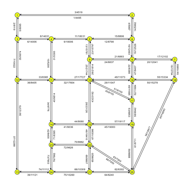
Figure 4: Equilibrium flows calculated by FW algorithm

Let $\varepsilon^{n}$ and $\varepsilon_{r}^{n}$ denote the summation of the error and the max relative error between each equilibrium link flow and the assignment link flow at $n_{th}$ iteration, namely:

$$\begin{array}[]{l}\varepsilon^{n}=\sum\limits_{i,j\in N}\varepsilon_{ij}^{n},~{}~{}~{}\forall i,j\in N\\ \varepsilon_{r}^{n}=\max\{\frac{{\varepsilon_{ij}^{n}}}{{Q_{ij}^{all}}}\},~{}~{}~{}\forall i,j\in N\end{array}$$ (29)

where $Q_{ij}^{all}$ denotes the equilibrium flow along link $M_{ij}$, $\varepsilon_{ij}^{n}$ denotes the error between equilibrium flow and the assignment flow at the $n_{th}$ iteration along link $M_{ij}$. The change of $\varepsilon$ and $\varepsilon_{r}$ during iterations are indicated in Figure 5. The summation of the error $\varepsilon$ and the maximum relative error $\varepsilon_{r}$ are monotone decreasing during iterations. The maximum relative error of each link flow $\varepsilon_{r}^{24}$ is no more than $10\%$ at the $24_{th}$ iteration. After 100 iterations, the maximum relative error of each link flow $\varepsilon_{r}^{100}$ is no more than $2\%$ and the summation of error between each equilibrium link flow and the assignment link flow $\varepsilon^{100}$ equals 54.2587.

Figure 5: The error and max relative error of each link flow during iterations

5 CONClUSIONS

To address UE traffic assignment problem, a modified Physarum-inspired model for UE traffic assignment is proposed in this paper. Considering the foraging behavior of Physarum, the equilibrium flows can be obtained when the Physarum can’t find a shorter travel time between each OD pair. The modified algorithm is more efficient in real traffic networks with two-way traffic characteristics and multiple OD pairs . By decomposing flows according to origin node, the flows from different OD pairs can be distinguished. Numerical examples are illustrated to show the rationality and convergence properties of the proposed algorithm.

In the future, one of our works is to use paralleled computing and the optimal model for the linear system of equations [55] to reduce computing time. Besides, the theoretical analysis of convergence is also our research topic.

References

- Bertsekas and Gafni [1982] D. P. Bertsekas, E. M. Gafni, Projection methods for variational inequalities with application to the traffic assignment problem, in: Nondifferential and Variational Techniques in Optimization, Springer, 1982, pp. 139–159.
- Papageorgiou [1990] M. Papageorgiou, Dynamic modeling, assignment, and route guidance in traffic networks, Transportation Research Part B: Methodological 24 (1990) 471–495.
- Ziliaskopoulos [2000] A. Ziliaskopoulos, A linear programming model for the single destination System Optimum Dynamic Traffic Assignment problem, Transportation Science 34 (2000) 37–49.
- Liu et al. [2010] Y. Liu, J. Bunker, L. Ferreira, Transit Users’ Route-Choice Modelling in Transit Assignment: A Review, Transport Reviews 30 (2010) 753–769.
- Du et al. [2016] W.-B. Du, X.-L. Zhou, O. Lordan, Z. Wang, C. Zhao, Y.-B. Zhu, Analysis of the chinese airline network as multi-layer networks, Transportation Research Part E: Logistics and Transportation Review 89 (2016) 108–116.
- Wardrop [1952] J. G. Wardrop, Some theoretical aspects of road traffic research, in: Inst Civil Engineers Proc London /UK/, pp. 72–73.
- Beckmann et al. [1956] M. J. Beckmann, C. B. Mcguire, C. B. Winsten, T. C. Koopmans, Studies in the economics of transportation, Economic Journal 26 (1956) 820–821.
- Chiou [2009] S. W. Chiou, An efficient algorithm for optimal design of area traffic control with network flows, Applied Mathematical Modelling 33 (2009) 2710–2722.
- Florian et al. [2009] M. Florian, I. Constantin, D. Florian, A new look at projected gradient method for equilibrium assignment, Transportation Research Record: Journal of the Transportation Research Board (2009) 10–16.
- Chiou [2010] S. W. Chiou, An efficient algorithm for computing traffic equilibria using transyt model, Applied Mathematical Modelling 34 (2010) 3390–3399.
- Lin and Leong [2014] D. Y. Lin, P. W. Leong, An n-path user equilibrium for transportation networks, Applied Mathematical Modelling 38 (2014) 667 C682.
- Leblanc et al. [1975] L. J. Leblanc, E. K. Morlok, W. P. Pierskalla, An efficient approach to solving the road network equilibrium traffic assignment problem, Transportation Research 9 (1975) 309–318.
- Ryu et al. [2014] S. Ryu, A. Chen, K. Choi, A modified gradient projection algorithm for solving the elastic demand traffic assignment problem, Computers & Operations Research 47 (2014) 61–71.
- Larsson and Patriksson [1992] T. Larsson, M. Patriksson, Simplicial decomposition with disaggregated representation for the traffic assignment problem, Transportation Science 26 (1992) 4–17.
- Jayakrishnan et al. [1994] R. Jayakrishnan, W. T. Tsai, J. N. Prashker, S. Rajadhyaksha, A faster path-based algorithm for traffic assignment, University of California Transportation Center (1994).
- Cheng et al. [2003] L. Cheng, Y. Iida, N. Uno, W. Wang, Alternative quasi-newton methods for capacitated user equilibrium assignment, Transportation Research Record: Journal of the Transportation Research Board (2003) 109–116.
- Sun et al. [1996] C. Sun, R. Jayakrishnan, W. Tsai, Computational study of a path-based algorithm and its variants for static traffic assignment, Transportation Research Record: Journal of the Transportation Research Board (1996) 106–115.
- Tatineni et al. [1998] M. Tatineni, H. Edwards, D. Boyce, Comparison of disaggregate simplicial decomposition and frank-wolfe algorithms for user-optimal route choice, Transportation Research Record: Journal of the Transportation Research Board (1998) 157–162.
- Bar-Gera [1999] H. Bar-Gera, Origin-based algorithms for transportation network modeling., National Institute of Statistical Sciences Research Park Nc (1999).
- Bar-Gera [2002] H. Bar-Gera, Origin-based algorithm for the traffic assignment problem, Transportation Science 36 (2002) 398–417.
- Dial [2006] R. B. Dial, A path-based user-equilibrium traffic assignment algorithm that obviates path storage and enumeration, Transportation Research Part B: Methodological 40 (2006) 917–936.
- Xu et al. [2008] M. Xu, A. Chen, Z. Gao, An improved origin-based algorithm for solving the combined distribution and assignment problem, European Journal of Operational Research 188 (2008) 354–369.
- Matteucci and Mussone [2013] M. Matteucci, L. Mussone, An ant colony system for transportation user equilibrium analysis in congested networks, Swarm Intelligence 7 (2013) 255–277.
- D Acierno et al. [2012] L. D Acierno, M. Gallo, B. Montella, An ant colony optimisation algorithm for solving the asymmetric traffic assignment problem, European Journal of Operational Research 217 (2012) 459–469.
- Sanchez-Medina et al. [2012] J. J. Sanchez-Medina, M. Diaz-Cabrera, M. J. Galan-Moreno, E. Rubio-Royo, User Equilibrium Study of AETROS Travel Route Optimization System, in: MorenoDiaz, R and Pichler, F and QuesadaArencibia, A (Ed.), Computer Aided Systems Theory - Eurocast 2011, PT II, volume 6928 of Lecture Notes in Computer Science, Springer-Verlag Berlin, Heidelberger Platz 3, D-14197 Berlin, Germany, 2012, pp. 465–472.
- Adamatzky [2007] A. Adamatzky, Physarum machines: encapsulating reaction–diffusion to compute spanning tree, Naturwissenschaften 94 (2007) 975–980.
- Adamatzky and Jones [2010] A. Adamatzky, J. Jones, Programmable reconfiguration of physarum machines, Natural Computing 9 (2010) 219–237.
- Adamatzky and Jones [2015] A. Adamatzky, J. Jones, On using compressibility to detect when slime mould completed computation, Complexity (2015).
- Stephenson and Stempen [1995] S. L. Stephenson, H. Stempen, Myxomycetes : a handbook of slime molds, Bioscience 45 (1995) 601–602.
- Nakagaki et al. [2000] T. Nakagaki, H. Yamada, Á. Tóth, Intelligence: Maze-solving by an amoeboid organism, Nature 407 (2000) 470–470.
- Tero et al. [2010] A. Tero, S. Takagi, T. Saigusa, K. Ito, D. P. Bebber, M. D. Fricker, K. Yumiki, R. Kobayashi, T. Nakagaki, Rules for biologically inspired adaptive network design., Science 327 (2010) 439–442.
- Bonifaci et al. [2012] V. Bonifaci, K. Mehlhorn, G. Varma, Physarum can compute shortest paths, in: Acm-Siam Symposium on Discrete Algorithms, p. 121 C133.
- Adamatzky [2012] A. Adamatzky, Slime mold solves maze in one pass, assisted by gradient of chemo-attractants., IEEE Transactions on Nanobioscience 11 (2012) 131–4.
- Wang et al. [2014] H. Wang, X. Lu, X. Zhang, Q. Wang, Y. Deng, A bio-inspired method for the constrained shortest path problem, The Scientific World Journal 2014 (2014).
- Zhang et al. [2014] X. Zhang, Y. Zhang, Y. Deng, An improved bio-inspired algorithm for the directed shortest path problem, Bioinspiration & Biomimetics 9 (2014).
- Wang et al. [2015] Q. Wang, X. Lu, X. Zhang, Y. Deng, C. Xiao, An anticipation mechanism for the shortest path problem based on Physarum polycephalum, International Journal of General Systems 44 (2015) 326–340.
- Adamatzky [2012] A. Adamatzky, Bioevaluation of world transport networks, Bioevaluation of World Transport Networks 43 (2012) 368.
- Adamatzky et al. [2013] A. Adamatzky, M. Lees, P. Sloot, Bio-development of motorway network in the netherlands: a slime mould approach, Advances in Complex Systems 16 (2013) 1250034.
- Tsompanas et al. [2014] M.-A. I. Tsompanas, G. C. Sirakoulis, A. I. Adamatzky, Physarum in silicon: the greek motorways study, Natural Computing (2014) 1–17.
- Evangelidis et al. [2015] V. Evangelidis, M. A. Tsompanas, G. C. Sirakoulis, A. Adamatzky, Slime mould imitates development of roman roads in the balkans, Journal of Archaeological Science Reports 2 (2015) 264–281.
- Schumann and Adamatzky [2011a] A. Schumann, A. Adamatzky, Logical modelling of physarum polycephalum, arXiv preprint arXiv:1105.4060 (2011a).
- Schumann and Adamatzky [2011b] A. Schumann, A. Adamatzky, Physarum spatial logic, New Mathematics and Natural Computation 7 (2011b) 483–498.
- Braund and Miranda [2013] E. Braund, E. Miranda, Music with unconventional computing: a system for physarum polycephalum sound synthesis, in: International Symposium on Computer Music Modeling and Retrieval, Springer, pp. 175–189.
- Miranda [2014] E. R. Miranda, Harnessing the intelligence of physarum polycephalum for unconventional computing-aided musical composition., IJUC 10 (2014) 251–268.
- Braund and Miranda [2015] E. Braund, E. Miranda, Music with unconventional computing: towards a step sequencer from plasmodium of physarum polycephalum, in: International Conference on Evolutionary and Biologically Inspired Music and Art, Springer, pp. 15–26.
- Zhang et al. [2013] Y. Zhang, Z. Zhang, Y. Deng, S. Mahadevan, A biologically inspired solution for fuzzy shortest path problems, Applied Soft Computing 13 (2013) 2356–2363.
- Zhang et al. [2014] X. Zhang, Q. Wang, A. Adamatzky, F. T. Chan, S. Mahadevan, Y. Deng, A biologically inspired optimization algorithm for solving fuzzy shortest path problems with mixed fuzzy arc lengths, Journal of Optimization Theory & Applications 163 (2014) 1049–1056.
- Jiang et al. [2015] W. Jiang, Y. Luo, X. Qin, J. Zhan, An improved method to rank generalized fuzzy numbers with different left heights and right heights, Journal of Intelligent & Fuzzy Systems 28 (2015) 2343–2355.
- Zhang et al. [2015] X. Zhang, A. Adamatzky, F. T. Chan, Y. Deng, H. Yang, X.-S. Yang, M.-A. I. Tsompanas, G. C. Sirakoulis, S. Mahadevan, A biologically inspired network design model, Scientific reports 5 (2015).
- Zhang [2015] X. Zhang, An Efficient Physarum Algorithm for Solving the Bicriteria Traffic Assignment Problem, International Journal of Unconventional Computing 11 (2015) 473–490.
- Tero et al. [2007] A. Tero, R. Kobayashi, T. Nakagaki, A mathematical model for adaptive transport network in path finding by true slime mold, Journal of theoretical biology 244 (2007) 553–564.
- Hansen [1959] W. G. Hansen, How accessibility shapes land use, Journal of the American Institute of planners 25 (1959) 73–76.
- Boyce et al. [2004] D. Boyce, B. Ralevic-Dekic, H. Bar-Gera, Convergence of traffic assignments: how much is enough?, Journal of Transportation Engineering 130 (2004) 49–55.
- Adamatzky and Jones [2008] A. Adamatzky, J. Jones, Towards physarum robots: computing and manipulating on water surface, Journal of Bionic Engineering 5 (2008) 348–357.
- Koutis et al. [2010] I. Koutis, G. L. Miller, R. Peng, Approaching optimality for solving sdd linear systems, in: Foundations of Computer Science (FOCS), 2010 51st Annual IEEE Symposium on, IEEE, pp. 235–244.